This article was downloaded by: [McGill University Library]On: 16 October 2014, At: 08:32Publisher: Taylor & FrancisInforma Ltd Registered in England and Wales Registered Number: 1072954 Registered office: Mortimer House,37-41 Mortimer Street, London W1T 3JH, UK

Electric Machines & Power SystemsPublication details, including instructions for authors and subscription information:http://www.tandfonline.com/loi/uemp19

A Novel Approach for Limit Cycle Analysis of anInterconnected Hydrothermal Power SystemChing-Tsai PAN a & Hong-Chan Chang ba Department of Electrical Engineering , National Tsing Hua University , Hsinchu, Taiwan,Republic of Chinab Department of Electrical Engineering , National Taiwan Institute of Technology , Taipei,Taiwan, Republic of ChinaPublished online: 24 Oct 2007.

To cite this article: Ching-Tsai PAN & Hong-Chan Chang (1988) A Novel Approach for Limit Cycle Analysis of an InterconnectedHydrothermal Power System, Electric Machines & Power Systems, 14:3-4, 231-247, DOI: 10.1080/07313568808909286

To link to this article: http://dx.doi.org/10.1080/07313568808909286

PLEASE SCROLL DOWN FOR ARTICLE

Taylor & Francis makes every effort to ensure the accuracy of all the information (the “Content”) containedin the publications on our platform. However, Taylor & Francis, our agents, and our licensors make norepresentations or warranties whatsoever as to the accuracy, completeness, or suitability for any purpose of theContent. Any opinions and views expressed in this publication are the opinions and views of the authors, andare not the views of or endorsed by Taylor & Francis. The accuracy of the Content should not be relied upon andshould be independently verified with primary sources of information. Taylor and Francis shall not be liable forany losses, actions, claims, proceedings, demands, costs, expenses, damages, and other liabilities whatsoeveror howsoever caused arising directly or indirectly in connection with, in relation to or arising out of the use ofthe Content.

This article may be used for research, teaching, and private study purposes. Any substantial or systematicreproduction, redistribution, reselling, loan, sub-licensing, systematic supply, or distribution in anyform to anyone is expressly forbidden. Terms & Conditions of access and use can be found at http://www.tandfonline.com/page/terms-and-conditions

A NOVEL APPROACH FOR LIMIT CYCLE ANALYSIS OF AN INTERCONNECTED HYDROTHERMAL POWER SYSTEM

CHING-TSAI PAN

Department of Electrical Engineering National Tsing Hua University Hsinchu, Taiwan Republic of China

HONG-CHAN CHANG

Department of Electrical Engineering National Taiwan Institute of Technology Taipei, Taiwan Republic of China

Abstract

A novel. approach which can predict limit cycle oscillat.ions of arbitrary control systems containing multiple nonlinearities is presented. First a widely convergent algorithm for findhg a limit cycle is presented. Then an efficient and systematic graphical approach is delineated for plotting the limit cycle loci on the parameter plane of interest. The attractive merits of this approach lie in its generality, simpJ.icity, und abi.lity to give a more complete picture about the parameter influence on the limit cycle. Besides, incorporating with the proposed method,, a quasi-static criterion is also derived for checking the stabil-ity of a limit cycle with little additional efforts. Finally, the propxed method is applied to the limit cycle analysis of a11

interco~ected hydrothermal power system to investigate the effects of prwleter changes on Li1n.i t cydes. Res11.lts of this study will not only enhance our. understanding of limit cyc1.e phenomenon but also provide power engineers an efficient means for the parameter coordination of Automatic Generation Control IAGCJ of power systems to alleviate the adverse effects caused by limi t cycli.ng.

1:t is known 11-51 that, speed governor deadband (DBJ tends to produce self sustained oscillations otherwise called limit cycles, and hence has a destnbilizing effect on t,he dynamic performarrce of AGC. Since existence of the limit cycle may incur unnecessary control action as well as the wear and tear on the system hardware 15,61, it is essential to investigate this phenomenon thoroughly so that a strategy may be taken to avoid or reduce the influence of this effect.

ln the past decades, there have been many papers published ,,l-2,5-lll dealing with .limit cyc1.e analysis of power system. In early works 11-21 , Concordia et. al. conducted an exact analog simulation to examine the influence that nor11.inearitj.e~ such as governor deadband may have on the existence of these sustained oscillations. This procedure works we.11 for specific cases but is awkward for parametric studies. Recently, the formal analytical approach usiw describing function technique as well. as Nyquist p1ol;s was applied to investigate limit c.vc.lif~g phenomenon in an isolated power system [6-91. This method is a graphical method in nature, and it is usually difficu.Lt bo kreat the

Electric Machines and Power Systems, 14:231-247, 1988 Copyright O 1988 by Hemisphere Publishing Corporation

Dow

nloa

ded

by [

McG

ill U

nive

rsity

Lib

rary

] at

08:

32 1

6 O

ctob

er 2

014

232 C.-T. PAN AND H.-C. CHANG

limit cycling problem of multiarea power systems including governor deadband. Except for simulation techniques [I-2,51, the number of published studies is relatively small regarding the limit cycle analysis of interconnected power systems. To the best of the author's knowledge, the work done by Pantalone [lo] may be the only one that successfully handled the limit cycle analysis of two interconnected steam power systems in an analytic way. However, this method is generally restricted to a certain class of structure and is difficult to extend to multiarea power systems with more than two units. A very recent research by Shahrodi et. al. [51 explored the nonlinearities including governor deadband on the dynamic behavior of AGC systems using a digital simulation technique. Like other simulation techniques, time-domain simulation by analog, digital or other hybrid methods are prohibitively expensive. Besides, these approaches are generally not able to give one a more complete picture about the parameter influence on the limit cycle. On the other hand, it is frequently desired to investigate the effects of parameter changes on the limit cycle. This poses an even more comp1icat.d problem. In view of this, A general approach for constructing limit cycle loci on parameter planes [I21 is presented, which constitutes an extension of earlier results by the present authors 1111. The proposed method can handle any number of general nonlinearities and is applicable to most nonlinear configurations which would be encountered in practice. Besides, the condition to determine the stability of limit cycles in multiple nonlinearity systems is also derived. By using the proposed method, stability of the limit cycle can be checked without much additional efforts.

The purpose of this paper is to present a systematic method to explore the influence of important system parameters on the limit cycling phenomenon of an interconnected hydrothermal power system. Special emphases are placed on the coordination of the frequency bias parameter B. in the area control error and integrator gain KIi of the supplementary 1

cont,roller in this hydrothennal system. Significantly, this study will enhance our common understanding of limit cycling in power systems, and some guidance for ,selection of AGC parameters will be suggested to alleviate the adverse effects caused by limit cycling.

2 Problem formulation

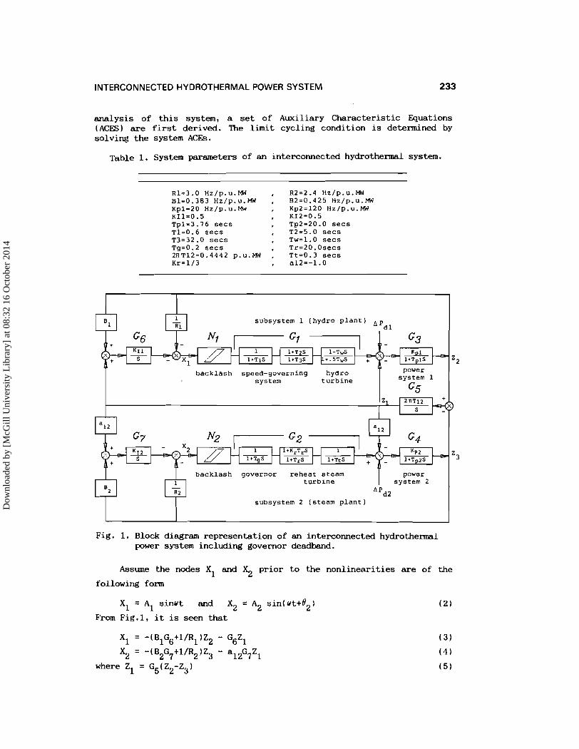
Consider an interconnected hydrothermal power system as shown in Fig.1 which includes governor deadbands [ 3 ] . The values of system parameters are listed in Table 1 131. As encountered in practical systems, it is assumed that the commonly used Sinusoidal Input Describing Function (SIDF) can be used to characterize the nonlinear elements of the interested systems. The describing functions N1 and N2 for the governor

deadband of areas 1 and 2 are:

where b and Ai denote half width of the governor deadband and the input

magnitude to the ith nonlinearity respectively. Under steady state, both areas are assumed in perfect synchronism, i.e., they have one c o m n system frequency. To demonstrate the proposed method for limit cycle

Dow

nloa

ded

by [

McG

ill U

nive

rsity

Lib

rary

] at

08:

32 1

6 O

ctob

er 2

014

INTERCONNECTED HYDROTHERMAL POWER SYSTEM 233

analysis of this system, a set of Auxiliary Characteristic Equations (ACES) are first derived. The limit cycling condition is determined by solving the system ACES.

Table 1. System parameters of an interconnected hydrothermal system.

R1=3.0 Hz/p.u.MW B1=0.383 Hz1p.u.W Kpl=2O Hz1p.u.W KI1.0.5 Tp1.3.76 secs T1=0.6 secs T3=32.0 secs Tg=0.2 secs 2IlT12=0.4442 p.U.MW Kr=1/3

R2=2.4 Hz/p.U.MW B2=0.425 Hz/p.u.MW Kp2=12O Hz/p.u.MW KI2=0.5 Tp2=20.0 secs T2=5.0 secs Tw=l.O secs Tr=2O.Osecs Tt=0.3 secs a12=-1.0

subsystem 1 (hydro plant) A Pdl

Cs Nf C, 1 G3

backlash speed-governing hydro power

system turbine system 1

r;l ? backlash governor reheat steam power turbine

A 'd2 subsystem 2 (steam plant)

Fig. 1. Block diagram representation of an interconnected hydrothemal power system including governor deadband.

Assume the nodes X and X prior to the nonlinearities are of the 1 2

following form

X1 = A sinut and X2 = A2 sin(~t+@~l 1 From Fig.1, it is seen that

Xl = -(B1G6+1/R1)Z2 - G6Z1 X2 = -(B2G7+1/R2)Z3 - a 12 G 7 Z 1

where Z = G ( Z -Z ) 1 5 2 3

Dow

nloa

ded

by [

McG

ill U

nive

rsity

Lib

rary

] at

08:

32 1

6 O

ctob

er 2

014

234 C.-T. PAN AND H.-C. CHANG

Similarly, one can also obtain two equations for the rest of the block diagrem

From Eqs. (5), (6) and (7), one can solve for Z 2 and z3

Thus, substituting Eqs. (a), ( 9 ) and (5) into Eqs. ( 3 ) and ( 4 ) to eliminate Z2 and Z3 yields the following auxiliary characteristic

equations :

I n the frequency domain, when the above two complex equations are used to j@ predict the limit cycles, X,=A,. X2=A2 e 2 and S = j u should be used. Note

- -, - - that there are equivalently four real equations with four unlmowns,namely A1' Y' A2 and @ 2 '

In fact, the problem of finding the limit cycle in a multiple nonlinearity systems with N nonlinearities can be reduced to solving a set of N complex ACES with 2N unknowns, which in the most general fonn can be expressed as 1121:

Note that the number of equations is equal to that of the nonlinear elements. In general, this dimension involved in this method is much less than that of using state space representation 113,141. Taking Fig.1 as an example, the dimension used by this method is only 4 whereas that used by references [13 ,14] is 11. However, to solve the resulting nonlinear systems of equations is still not a simple matter at all. The commonly used Newton-Raphson method usually requires a rather good initial guess to achieve a converged solution. Unfortunately, this good initial guess is not available in the limit cycle analysis. Besides, Eq. (12 ) is generally very nonlinear. To overcome these difficulties, a recently developed homotopy method [151, which basically possesses global convergence characteristic, is introduced in the following section.

Dow

nloa

ded

by [

McG

ill U

nive

rsity

Lib

rary

] at

08:

32 1

6 O

ctob

er 2

014

INTERCONNECTED HYDROTHERMAL POWER SYSTEM

3 Limit cycle analysis on the parameter plane

A widely converaent algorithm for solvine F(X)=O

As a rough explanation, consider the problem of solving

h e can construct a linear homotopy H

It is seen that the solution of H=O for all tE[O,l] forms a space trajectory. At t=O, the solution is a trivial one and at t=l, the solution is the desired one. Thus, one can trace along the space curve defined by H=O from t=O to t=l to obtain the desired solution. To track this curve, one approach is to integrate the following differential equation, which is obtained by taking the total time derivative of H(X,t)=O, using the Runge Kutta method:

Thus, through this widely convergent algorithm, it is not difficult to find the desired limit cycle. As will be seen later, in actually constructing the limit cycle loci on a specified a-b parameter plane, the nonlinear equations F and the unknown vector X in Eq. (14) are expressed as

X=[a,b,A2,O2, .,%,ON] T T

F=rRe(F1),Im(F1),Re(F2),Im(F2),. . . ,Re(FN),Im(FN)l It is desired that, with given A1 and w , to find X such that

complex set of ACEs in Eq. (12) are satisfied.

Construction of limit cycle loci

(16)

the

Although, one can use the previous approach to find the resulting limit cycle for each new set of parameters, it would be difficult to have an overall picture about the variation tendency. For this purpose, this paper presents a systematic method for plotting the limit cycle loci on the parameter planes. The limit cycle loci on a parameter plane consists of a family of constant A1 curves as well as constant u curves. Each

constant A curve is obtained by solving the parameter coordinates from 1 -

the previous ACEs as u is varied. Similarly, each constant u curve is obtained by finding the parameter coordinates from the ACES as A1 is

varied. Thus, on the parameter plane, the intersecting points of these two families of curves constitute the desired limit cycle loci. Therefore, within the interested parameter range, the overall tendency of

Dow

nloa

ded

by [

McG

ill U

nive

rsity

Lib

rary

] at

08:

32 1

6 O

ctob

er 2

014

236 C.-T. PAN AND H.-C. CHANG

the parameter influences can be seen clearly. Consider the construction of a constant amplitude curve on a

particular parameter plane, say the a-b plane. The amplitude of the input sinusoid of the reference nonlinear element is chosen as a constant value and the limit cycle frequency is considered as an independent variable. Then Eq. ( 1 2 ) can be rewritten as

where the arguments of FRi and FIi are omitted for simplicity.

Differentiating Eq. ( 1 7 ) with respect to u yields

Separating the real and the imaginary parts of Eq.

which can be written in a more simple form as

---- ,...,- - aa ab J A ~ a02 a $0,

( 1 8 )

( 1 8 ) yields

- do

Dow

nloa

ded

by [

McG

ill U

nive

rsity

Lib

rary

] at

08:

32 1

6 O

ctob

er 2

014

INTERCONNECTED HYDROTHERMAL POWER SYSTEM 237

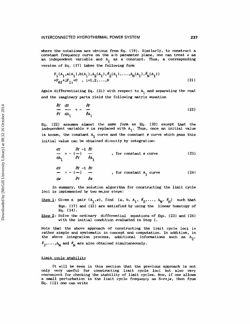
where the notations are obvious from Eq. (19). Similarly, to construct a constant frequency curve on the a-b parameter plane, one can treat w as an independent variable and A1 as a constant. Thus, a corresponding

version of Eq. (17) takes the following form

Again differentiating Eq. (21) with respect to A1 and separating the real

and the imaginary parts yield the following matrix equation

Eq. (22) assumes almost the same form as Eq. (20) except that the independent variable u is replaced with A1. Thus, once an initial value

is known, the constant A1 curve and the constant u curve which pass this

initial value can be obtained directly by integration:

dY iF -1 8F - = - (-) - , for constant Y curve (23)

dA1 ay aal

dY aF -1 iF - = - (-) - , for constant A1 curve (24)

do 8~ JY

In summary, the solution algorithm for constructing the limit cycle loci is implemented by two major steps:

Stepl: Given a pair (Al, u ) , find (a, b, A1, e2,. . . , %, ON) such that -

Eqs. (17) and (21) are satisfied by using the linear hornotopy of Eq. ( 1 4 ) .

Steu 2: Solve the ordinary differential equations of Eqs. (23) and (24) with the initial condition evaluated in Step 1.

Note that the above approach of constructing the limit cycle loci is rather simple and systematic in concept and computation. In addition, in the above integration process, additional informations such as A2,

e2,. . . ,% and flN are also obtained simultaneously.

. . cle stab-

It will be seen in this section that the previous approach is not only very useful for constructing limit cycle loci but also very convenient for checking the stability of limit cycles. Now, if one allows a small perturbation in the limit cycle frequency as S=o+ju , then from Eq. (12) one can write

Dow

nloa

ded

by [

McG

ill U

nive

rsity

Lib

rary

] at

08:

32 1

6 O

ctob

er 2

014

C.-T. PAN AND H.-C. CHANG

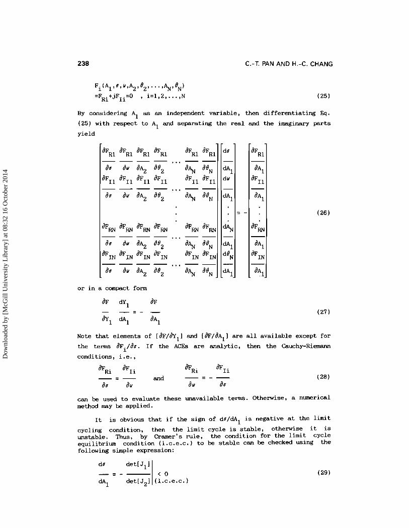
By considering A as an independent variable, then differentiating Eq. 1 (25) with respect to A1 and separating the real and the imaginary parts

yield

---- ... -- a. aw a ~ , as, a% BFIl 851 aF~l aF1l aFIl aFIl

. . . aa ao a~~ as, a% a e ~

---- ... - - a. au a ~ , ae, a% 'IN a F ~ ~ &IN a F ~ ~ &IN

... a. au a ~ , as,

or in a compact form

Note that elements of [ aF/8Y1 1 and [aF/aA1 I are all available except for the terms aFi/ao. If the ACES are analytic, then the Cauchy-Riemann

conditions, i.e.,

- - - - and - = - - ar au au aa

can be used to evaluate these unavailable terms. Otherwise, a numerical method may be applied.

It is obvious that if the sign of do/dA1 is negative at the limit

cycling condition, then the limit cycle is stable, otherwise it is unstable. Thus, by Cramer's rule, the condition for the limit cycle equilibrium condition (1.c.e.c.) to be stable can be checked using the following simple expression:

Dow

nloa

ded

by [

McG

ill U

nive

rsity

Lib

rary

] at

08:

32 1

6 O

ctob

er 2

014

INTERCONNECTED HYDROTHERMAL POWER SYSTEM

where det[J1l and det[J21 are evident from Eq. (26).

4 mects of mrameter variations

To investigate the influence of parameter variations on the existence of limit cycle and show deeper insight into its characteristics, different parameter planes showing limit cycling are constructed by the presented method. In the past, although there are some papers addressing the limit cycling problem of an isolated area power system, the lack of a general analytic method for the study of this problem in interconnected power systems blocks our overall understanding of the peculiar nature of limit cycles. On the other hand, this study will not only provide one with qualitative and quantitative analysis results of limit cycles in an interconnected hydrothermal system but also provide analytical guidance to alleviate the unfavorable effects of limit cycling. Before proceeding, it should be noted that each plot of limit cycle loci is constructed by varying parameters examined within the proper range and keeping all other parameters fixed at values as shown in Table 1. In all plots the locus of dotted line represent constant frequency curves while solid lines represent constant amplitude curves.

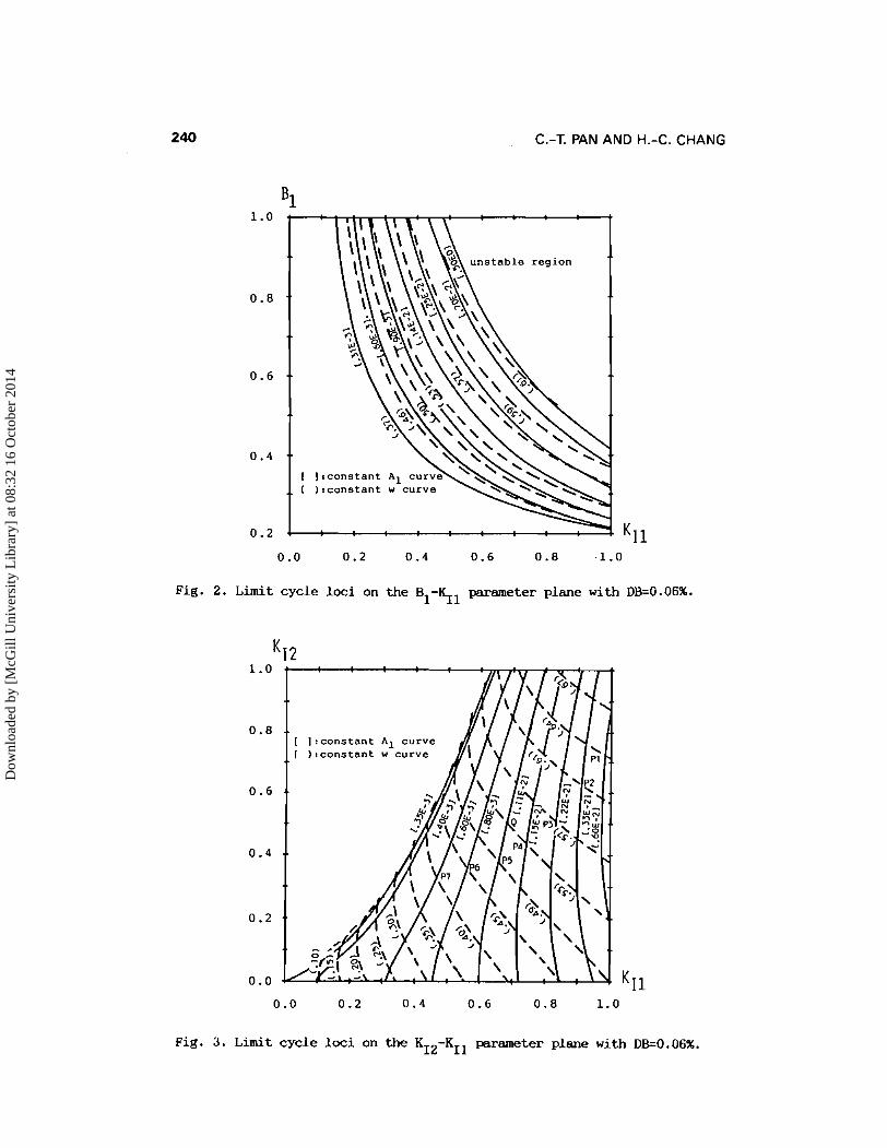
B1-KI1 parameter plane

Since the frequency bias parameter B in the area control error and integrator gain KT of the supplementary controller are two important

-

feedback gains for power system operation and control, the analysis is first conducted on this plane. Fig. 2 shows the effect of variations of B1 and KI1 on the limit cycle characteristics.Note that that increasing - - -

B1 or K will result in a larger amplitude and frequency of the limit I1 cycle, and may even cause the system to be unstable if B1 or KI are too 1 large. Therefore, the reduction of frequency bias B or integrator gain 1 KI1 will suppress the tendency to limit cycle. The effect of varying KI1

appears to be in agreement with conclusions reached by Wu and Pantalone [6 ,9] , and that of varying B1 verifies the observations noted by Taylor [ 161.

K12-KI1 parameter plane

Another aspect to be examined is the influence of integrator gains in different areas on the limit cycle. As shown in Fig.3, increasing K I1 will enhance the limit cycling, while increasing K will suppress the I2 limit cycling. Decreasing K will result in a smaller magnitude and I1 lower frequency of limit cycle. However, decreasing K will result in a I2 larger magnitude but lower frequency of limit cycle. It is noted that increasing the integrator gain KT produces a tendency to instability

I

under the governor deadband effect for a single area system. Yet, for interconnected hydrothermal systems, the influence of integrator gains KI1 and K12 becomes more complicated. Fig. 3 can help coordinate the

Dow

nloa

ded

by [

McG

ill U

nive

rsity

Lib

rary

] at

08:

32 1

6 O

ctob

er 2

014

C.-T. PAN AND H.-C. CHANG

0.0 0.2 0.4 0.6 0.8 .1.0

Fig. 2. Limit cycle loci on the B1-KI1 parameter plane with DB=0.06%.

0.0 0.2 0.4 0.G 0.8 1.0

Fig. 3. Limit cycle loci on the K12-KI1 parameter plane with DB=0.06%.

Dow

nloa

ded

by [

McG

ill U

nive

rsity

Lib

rary

] at

08:

32 1

6 O

ctob

er 2

014

INTERCONNECTED HYDROTHERMAL POWER SYSTEM 241

integrator gains in interconnected payer systems to suppress the limit cycling to some restricted range of amplitude and frequency.

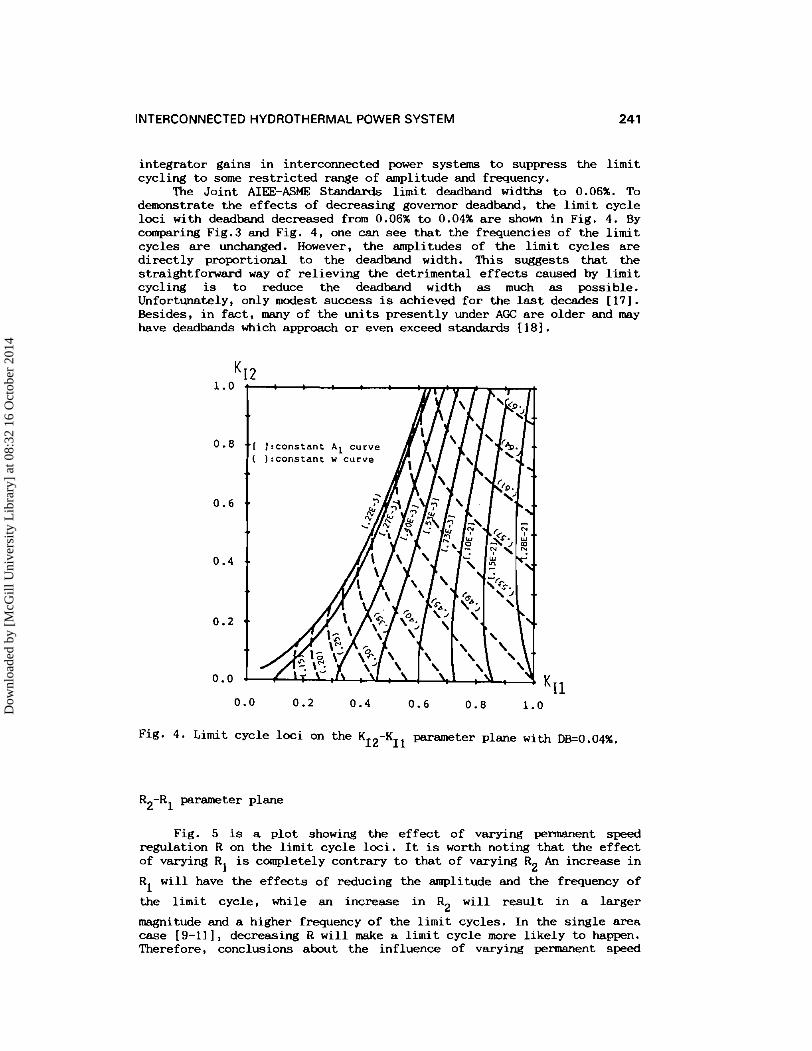
The Joint AIEE-ASME Standards limit deadband widths to 0.06%. To demonstrate the effects of decreasing governor deadband, the limit cycle loci with deadband decreased from 0.06% to 0.04% are shown in Fig. 4. By comparing Fig.3 and Fig. 4, one can see that the frequencies of the limit cycles are unchanged. However, the amplitudes of the limit cycles are directly proportional to the deadband width. This suggests that the straightforward way of relieving the detrimental effects caused by limit cycling is to reduce the deadband width as much as possible. Unfortunately, only modest success is achieved for the last decades [li']. Besides, in fact, many of the units presently under AGC are older and may have deadbands which approach or even exceed standards 1181.

Fig. 4. Limit cycle loci on the K12-KI1 parameter plane with DB=0.04%.

R -R parameter plane 2 1

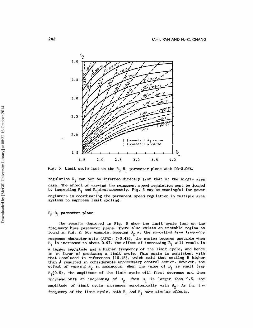
Fig. 5 is a plot showing the effect of varying pennanent speed regulation R on the limit cycle loci. It is worth noting that the effect of varying R is completely contrary to that of varying R An increase in 1 2 R1 will have the effects of reducing the amplitude and the frequency of

the limit cycle, while an increase in R2 will result in a larger

magnitude and a higher frequency of the limit cycles. In the single area case [9-111, decreasing R will make a limit cycle more likely to happen. Therefore, conclusions about the influence of varying pennanent speed

Dow

nloa

ded

by [

McG

ill U

nive

rsity

Lib

rary

] at

08:

32 1

6 O

ctob

er 2

014

C.-T. PAN AND H . 4 . CHANG

Fig. 5. Limit cycle loci on the R -R parameter plane with DB=0.06%. 2 1

regulati.on R; can not be inferred directly from that of the single area I

case. The effect of varying the permanent speed regulation must be judged by inspecting R1 and R2simultaneously. Fig. 5 may be meaningful for power

engineers in coordinating the pennsnent speed regulation in multiple area systems to suppress limit cycling.

B -B parameter plane 2 1

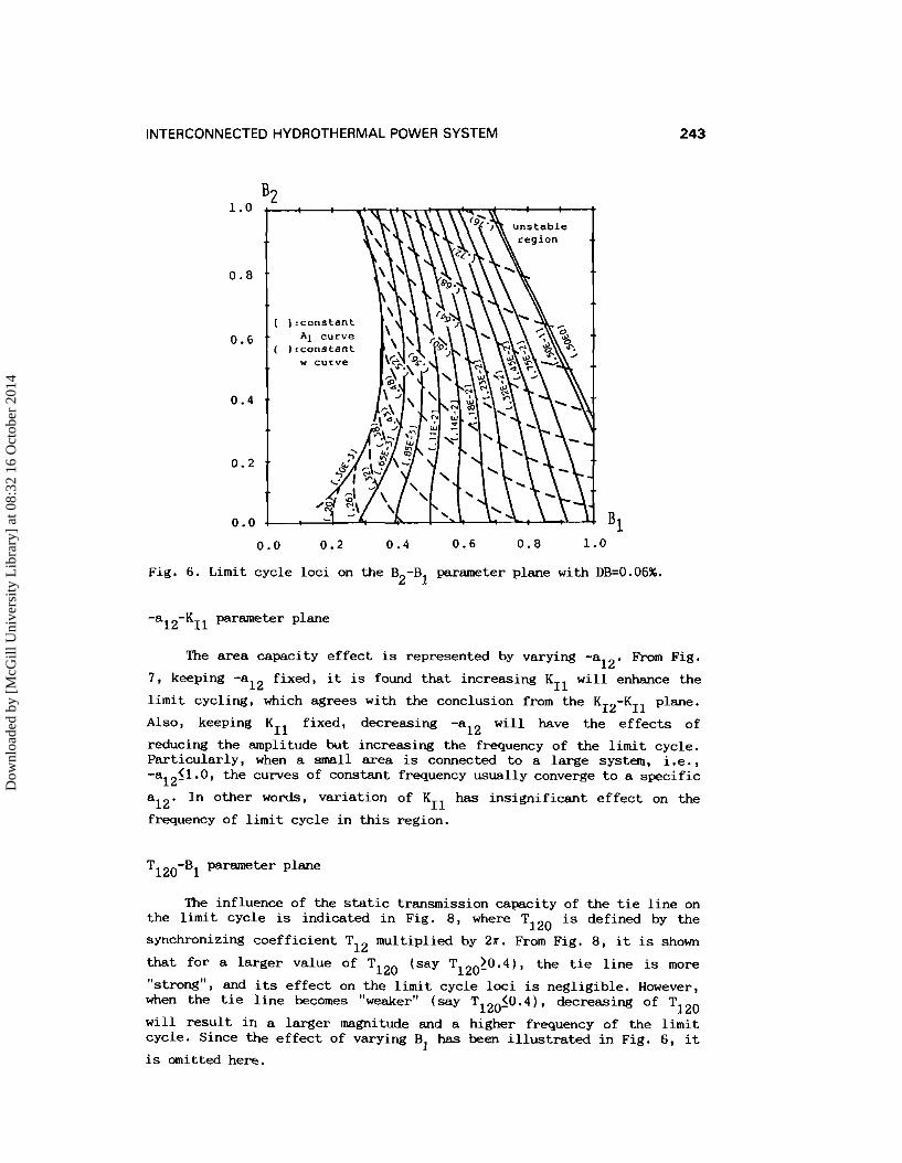
The results depicted in Fig. 6 show the limit cycle loci on the frequency bias parameter plane. There also exists an unstable region as found in Fig. 2. For example, keeping B2 at the so-called area frequency

response characteristic (AFRC) 8=0.425, the system becomes unstable when B, is increased to about 0.97. The effect of increasing B, will result in - a larger magnitude and a higher frequency of the limit cycle, and hence is in favor of producing a limit cycle. This again is consistent with that concluded in references [16,181, which said that setting B higher than 8 resulted in considerable unnecessary control action. However, the effect of varying B2 is ambiguous. When the value of B1 is small (say

-

B1<0.6), the amplitude of the limit cycle will first decrease and then

increase with an increasing of B2. When B1 is larger than 0.6, the

amplitude of limit cycle increases monotonically with B2. As for the

frequency of the limit cycle, both B2 and B1 have similar effects.

Dow

nloa

ded

by [

McG

ill U

nive

rsity

Lib

rary

] at

08:

32 1

6 O

ctob

er 2

014

INTERCONNECTED HYDROTHERMAL POWER SYSTEM

0.0 0.2 0.4 0.6 0.8 1.0

Fig. 6. Limit cycle loci on the B -B parameter plane with DB=0.06%. 2 1

-al2-KIl parameter plane

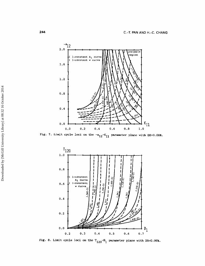
The area capacity effect is represented by varying -al2. From Fig.

7, keeping -a fixed, it is found that increasing KI1 will enhance the 12 limit cycling, which agrees with the conclusion from the K12-KI1 plane.

Also, keeping KI1 fixed, decreasing -al2 will have the effects of

reducing the amplitude but increasing the frequency of the limit cycle. Particularly, when a small area is connected to a large system, i.e., -a <1.0, the curves of constant frequency usually converge to a specific 12-

a12. In other words, variation of KI1 has insignificant effect on the --

frequency of limit cycle in this region.

TlZ0-B1 parameter plane

The influence of the static transmission capacity of the tie line on the limit cycle is indicated in Fig. 8, where TlZ0 is defined by the

synchronizing coefficient T12 multiplied by 2s. From Fig. 8, it is shown

that for a larger value of TIZO (say T >0.4), the tie line is more 120- "strong", and its effect on the limit cycle loci is negligible. However, when the tie line becomes "weaker" (say T120<0.4), decreasing of T

120 will result in a larger magnitude and a higher frequency of the limit cycle. Since the effect of varying B1 has been illustrated in Fig. 6, it

is omitted here.

Dow

nloa

ded

by [

McG

ill U

nive

rsity

Lib

rary

] at

08:

32 1

6 O

ctob

er 2

014

C.-T. PAN AND H.-C. CHANG

0.0 0.2 0 . 4 0.6 0.8 1.0

Fig. 7. Limit cycle loci on the -a 12-K11 parameter plane with DB=0.06%.

Fig. 8.

Dow

nloa

ded

by [

McG

ill U

nive

rsity

Lib

rary

] at

08:

32 1

6 O

ctob

er 2

014

INTERCONNECTED HYDROTHERMAL POWER SYSTEM

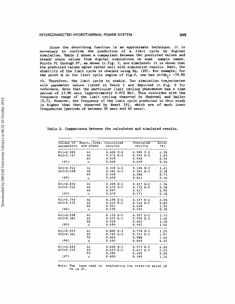
Since the describing function is an approximate technique, it is necessary to confirm the prediction of a limit cycle by digital simulation. Table 2 shows a comparison between the predicted values and steady state values from digital simulations on some sample cases. Points P1 through P7, as shown in Fig. 3, are simulated. It is shown that the predicted values agree rather well with simulation results. Next, the stability of the limit cycle is checked using Eq. (29). For example, for the point Q in the limit cycle region of Fig.3, one has dr/dA1= -74.85

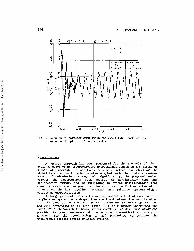
<O. Therefore, the limit cycle is stable. Two simulation trajectories with parameter values listed in Table 1 are depicted in Fig. 9 for reference. Note that the particular limit cycling phenomenon has a time period of 13.96 secs (approximately 0.072 Hz). This coincides with the frequency range of the limit cycling observed by Shahrodi and Bailey [5,7]. However, the frequency of the limit cycle predicted in this study is higher than that observed by Ewert [6], which are of much lower frequencies (periods of between 30 secs and 90 secs).

Table 2. Comparisons between the calculated and simulated results.

Values of Ampli.,freq. Calculated Shulated Error parameters and phase results results

Note: The base used in evaluating the relative error of 0 2 is 2n.

Dow

nloa

ded

by [

McG

ill U

nive

rsity

Lib

rary

] at

08:

32 1

6 O

ctob

er 2

014

C.-T. PAN AND H.-C. CHANG

Fig. 9. Results of computer simulation for 0.001 p.u. load increase in area-one (applied for one second).

A general approach has been presented for the analysis of limit cycle behavior of rm irlLercomected hydrothermal system on the parameter planes of interest. In addition, a simple method for checking the stability of a limit cycle is also adapted such that only a minimum amount of calculation is required. Significantly, the proposed method removes the restrictions with respect to nonlinearity type and nonlinearity number, and is applicable to system configurations most commonly encountered in practice. Hence, it can be further extended to investigate the limit cycling phenomenon in a multiarea systems with a variety of characteristics.

Although parts of the results are consistent with that concluded in single area system, some disparities are found between the results of an isolated area system and that of an interconnected power system. The analytic investigation of this paper will help better understand the 1i.mit cycle phenomenon in power system control. Besides, such study can provide the power engineers with more sound theoretical and analytic guidance for the coordination of AGC parameters to relieve the unfavorable effects caused by limit cycling.

Dow

nloa

ded

by [

McG

ill U

nive

rsity

Lib

rary

] at

08:

32 1

6 O

ctob

er 2

014

INTERCONNECTED HYDROTHERMAL POWER SYSTEM 247

References

1. C. Concordia, L. K. Kirchmayer and E. A. Szymanski, "Effect of speed governor deadband on tie-line power and frequency control perfonn- ance." AIEE Trans., vol. 76, pp. 429-435, 1957.

2. L. K. Kirchmayer, b, John Wiley, 1959.

3. S. C. Tripathy, G. S. Hope and 0. P. Malik, "Optimization of load- frequency control parameters for power systems with reheat steam turbines and governor deadband nonlinearities." IEE Pmc. C, Gen., Trans. & Distrib., vol. 129, pp. 10-15, 1982.

4 . S. C. Tripathy, T. S. Bhatti, C. S. Jha, 0. P. Malik and G. S. Hope, "Sampled data automatic generation control analysis with reheat steam turbines and governor dead-band effects." IEEE Trans., vol. PAS-103, pp. 1045-1051, 1984.

5. K. B. Shahrodi and A. Morched, "Dynamic behavior of AGC systems in- cluding the effects of nonlinearities. " IEEE Trans. , vol. PAS-104, pp. 3409-3415, 1985.

6. 1). K. Pantalone and D. M. Piegza, "Limit cycle analysis of hydro- electric systems." IEEE Trans., vol. PAS-100, pp. 629-638, 1981.

7. J. M. Bailey and G. F. Pierce, "Effects of nonlinearities on gov- ernor performance at BULL RUN steam plant." Roc. of the 7th Annual South-eastern Symposium on System Theory, pp. 137-138, Alabama, 1975.

8. J. M. Bailey and G. F. Pierce, "Backlash and rate saturation effects on governor performance at the BULL RUN steam plant." Proc. of IEEE South-eastern Region 3 Conference on Engineering in a Changing Econ- omy, pp. 10-12, South Carolina, 1976.

9. F. F. Wu and V. S. Dea, "Describing function analysis of automatic control system with governor deadband." Electric Power System Research, vol. 1, p!. 113-116, 1977/78.

)lo. D. K. Pantalone, Backlash describing function analysis for two steam areas." IEEE International Control Conference on Electrical Ehergy, pp. 13-15, Oklahoma City, 1981.

11. H. C. Chang, C. T. Pan, C. C. Wei and C. L. Huang, "Limit cycle analysis of hydroelectric systems: a new approach." Journal of Electric Power System Research, vol. 11, no. 2, pp. 49-59, 1986.

12. H. C. Chang, C. T. Pan, C. L. Huang and C. C. Wei, "A general approach for constructing the limit cycle loci of multiple- nonlinearity systems." IEEE Trans. Automat. Contr., vol. AC-32, pp. 845-848, Sep. 1987.

13. S. G. Abel and N. K. Cooperrider, "An algorithm for nonlinear system analysis and application to rail vehicle dynamics." F'roc. of the 1983 American Control Conference, pp. 257-262, June 1983.

14. A. A. Aderibigbe and J. K. Hedrick, "Limit cycle computation and stability for multivariable nonlinear systems." Pmc. of the 1984 American Control Conference, pp. 803-807, June 1984.

15. T. Y. Li, "Lecture on the numerical method of finding solutions of nonlinear equations." Lecture 1-4, seminar of Num. Analy. , held in Chiao-Tung Univ., Taiwan, 1983.

16. C. W. Taylor, K. Y. Lee and D. P. Dave, "Automatic generation cont- rol analysis with governor deadband effects." IEEE Trans., vol. PAS-98, pp. 2030-2036, 1979.

17. C. Concordia, Discussion of Reference 6. 18. D. N. Ewart, Discussion of Reference 16.

Manuscript received in final form March 29, 1988 Request reprints from Hong-Chan Chang

Dow

nloa

ded

by [

McG

ill U

nive

rsity

Lib

rary

] at

08:

32 1

6 O

ctob

er 2

014