A novel extension of Generalized Low-RankApproximation of Matrices based on multiple-pairs of

transformations

Soheil Ahmadia, Mansoor Rezghia,∗

aDepartment of Computer Science, Tarbiat Modares University, Tehran, Iran

Abstract

Dimension reduction is a main step in learning process which plays a es-

sential role in many applications. The most popular methods in this field like

SVD, PCA, and LDA, only can apply to vector data. This means that for

higher order data like matrices or more generally tensors, data should be fold

to a vector. By this folding, the probability of overfitting is increased and also

maybe some important spatial features are ignored. Then, to tackle these is-

sues, methods are proposed which work directly on data with their own format

like GLRAM, MPCA, and MLDA. In these methods the spatial relationship

among data are preserved and furthermore, the probability of overfitiing has

fallen. Also the time and space complexity are less than vector-based ones.

Having said that, because of the less parameters in multilinear methods, they

have a much smaller search space to find an optimal answer in comparison with

vector-based approach. To overcome this drawback of multilinear methods like

GLRAM, we proposed a new method which is a general form of GLRAM and

by preserving the merits of it have a larger search space. We have done plenty

of experiments to show that our proposed method works better than GLRAM.

Also, applying this approach to other multilinear dimension reduction methods

like MPCA and MLDA is straightforward.

Keywords: Machine learning, Matrix data classification, Kronecker product,

∗Corresponding authorEmail address: rezghi@modares.ac.ir (Mansoor Rezghi)

1

arX

iv:1

808.

1063

2v1

[cs

.LG

] 3

1 A

ug 2

018

Dimensionality reduction, SVD, PCA, GLRAM

1. Introduction

Machine learning (ML) is one of the most important concepts in Computer

Science which has many applications in the real world such as face recognition[1],

image processing[2], criminal recognition[3], medical images[4], computer vision[5],

data mining[6], etc. ML examines the methods which can learn from data in

order to improve the machine’s operating in different aspects. Data are usually

considered as a vector in ML so to apply well-known ML algorithms like SVM

[7], LDA[8], PCA[9], SVD[10] to data with the matrix or tensor structure, we

have to fold these data into a vector format. This folding causes two major

problems. At first, by converting a matrix or tensor to a long (wide) vector, the

number of free variables will be increased sharply, which can make overfitting

in the model. Also in vectorizing on some data like images, the spatial rela-

tionship among features are not considered, in other words, each datum treated

individually[11]. For example, a grayscale image represented by m × n matrix

in this approach will be reshaped to an nm vector. Therefore, not only we have

many free variables but also the local spatial relations among pixels of images

are not considered.

After a while in order to tackle vector-based methods drawbacks, another

approach considering data in their original format has been proposed which is

known as the multi-linear(tensor-based) learning[12][13]. In this approach, data

do not need to be reformulated anymore, and so by considering data in their

original format, the spatial relationship between data will be preserved.[11] Fur-

thermore, in contrast with vector-based methods, other methods based on tensor

representation have much less free variables which can reduce the computational

complexity and also probability of overfitting.[14] For instance, for a m×n ma-

trix with tensor-based methods, we have only m + n free variables which are

less than nm in vector-based viewpoint. By developing of this approach, some

tensor-based learning methods like MPCA[15], MLDA[16], STM[17], have been

2

represented as tensor counterparts of PCA, LDA, SVM, respectively[18][19].

Despite of mentioned appropriate properties, these methods have some prob-

lems, either. The main problem of tensor-based methods is their limited search

space which is only a subset of vector-based one. So, the probability of finding

an optimal answer in such a small search space is less than the large feasible

region in traditional methods, by far.

The problem of dimension reduction has become an essential tool for re-

moving noise from data[20], reduce redundancy[21], and feature extraction[22].

One of the main DR methods that are also related to well-known PCA, is

SVD.[23][24] However, since data should be vectorized in SVD and in this case,

the time and space complexities will be increased dramatically, it does not work

well in some data like images. For this reason, several algorithms have been pro-

posed in the last decade to deal with the high complexity of SVD computation,

where the best one of them was GLRAM[25] representing each datum in its

original format, instead of a vector, and by one pair of left and right projector,

transfer the data into a smaller subspace.

Furthermore in recent years some variants of this method has been proposed.

For example since at each iteration of GLRAM two SVD should be computed,

this increases the time complexity. The authors in[26] show that instead of

SVD, its approximation by Lanczos could be used which improves its speed.

Although GLRAM has less complexity than SVD, its search space is smaller.[25]

So, the probability of finding an optimal answer has been reduced. In this pa-

per we proposed a method that by applying k-pair left and right projectors to

data expand this limited space to find a more accurate answer. This idea is

inspired by a new approach which Hou et al, have stated in their paper[27].

They proposed a multiple-rank multilinear SVM for classification, that expands

the search space of STM in order to gain a more accurate answer same as SVM.

Theoretically, we show that by this idea the space of search is increased and

so the quality of approximation in this method will be better than GLRAM. Also

experiments show the quality of the method based on approximation and classi-

fication results. So, our experiments illustrated that in the proposed method, we

3

can find a better answer for the low-rank approximation. Not to mention that

through our approach, it is easy to show that the same idea could be applied

to other tensor based dimension reduction methods like MPCA and MLDA, in

the near future.

The rest of this paper is organized as follows. In section 2, we analyze SVD

and GLRAM methods and the relationship between them. In section 3, we

present our proposed method. Next, the experimental results will be discussed

in section 4. And finally, the conclusion stated in section 5.

2. Related works

In real applications, data usually contains some noisy and redundant features

which affect the quality of the learning process, especially for high dimensional

data. Dimension Reduction (DR) is a process that by transforming data into

a lower dimension, tries to eliminate noises and redundancy of data[18][23].

Therefore, the occurrence of curse of dimensionality and other undesired prop-

erties of high-dimensional spaces will be reduced, which has an important role

in many applications.[28].

In the last decade, a large number of DR techniques with different viewpoints

like PCA, SVD, Fisher LDA and so on, have been investigated. Similar to

other ML methods the input of the mentioned DR methods should be in vector

format and so data types like images and videos (Matrix or Tensor) should be

represented as a vector. This folding of high-order data to vector not only has

a high complexity but also can causes losing some important spatial relations

of the data. In recent years some multilinear versions of the mentioned DR

methods have been proposed which are able to work with high-order data like

matrices and tensors directly without reshaping them to vector i.e. MPCA,

4

GLRAM and Multilinear LDA are the tensor versions of PCA, SVD, and LDA

respectively.

The main advantage of the multilinear methods could be summarized as follows:

• They maintain the structure and so the spatial relations of data.

• The parameters of the multilinear methods are less than the vector-based

ones and so the computational complexity becomes less than linear meth-

ods. Also, for multilinear methods, the probability of occurrence of over-

fitting will be decreased

However, the multilinear methods are not convex typically, and also their

search space is much smaller than linear ones. So the solution obtained might

be far from the optimal answer.

In this paper, we expand the search space of GLRAM, which can cause to gain

better results. It should be mentioned that this approach could be applied to

other multilinear DR methods, too.

2.1. Linear DR methods based on low-rank approximation

PCA and SVD are the main DR methods that are related to each other. Let

X = [x1, ..., xN ] ∈ Rn×N became a centralized data set. The principal compo-

nent analysis (PCA) project the data from Rn to Rk, (k � n), by orthogonal

transformation W such that the variance of the projected data Y = WX will

be maximized.

It is easy to show that this can be formulated as follows:

maxW

trace(WTXXTW ) (1)

s.t. WTW = I.

It is known that the eigenvectors of corresponding of the first k eigenvalues of

XXT are the solution to Eq.1. Hence, if X = UΣV T be the Singular Value

Decomposition (SVD) of X, the first left singular vectors Uk = [u1, ..., uk] are

5

the first eigenvectors of XXT and so W = Uk.[24] Then, Yk = UTk X becomes

projected data. By SVD , it is clear that the projected data Yk becomes

Yk = UTk X = ΣkV

Tk , (2)

where Σk = diag(σ1, σ2, ..., σk).

In addition, the projection could be interpreted with another viewpoint. Since

Xk = UkΣkVTk = WYk, is the best rank-k approximation of X, so we found that

Yk is a reduced form of original data X such that have the least construction

error and, the PCA equals to the following problem

minYk,W

‖X −WYk‖2F (3)

s.t. WTW = I.

Therefore, the PCA and SVD dimension reduction also could be rewritten

as follows:

minW,Y

N∑i=1

‖xi −Wyi‖2F (4)

s.t. WTW = I.

It should be mentioned that for General data matrix X, where is not cen-

tralized, the SVD on X = [x1 − µ, x2 − µ, ..., xN − µ] is equal to PCA on A

where µ is the mean of the data.

2.2. Generalized low-rank approximations

Nowadays by increasing the usage of matrix datasets, the SVD (PCA) could

not be used directly on data. Now, If we have a dataset like {A1, ..., AN} where

6

Ai ∈ Rn1×n2 , then to apply SVD (PCA), every matrix Ai should be fold to

vector as follows:

ai = V ec(Ai) =[ai

T

1 , aiT

2 , ..., aiT

n2

]T, (5)

where aij is the j-th column of matrix Ai.

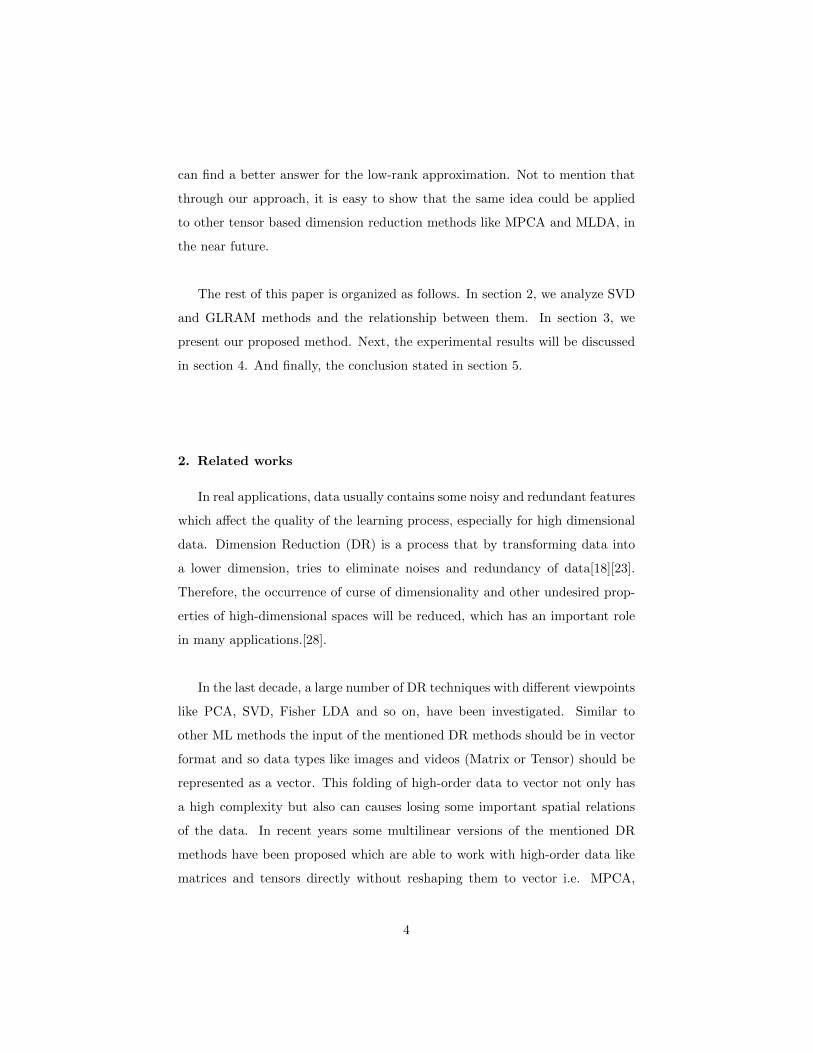
It is obvious that this folding maybe destroys some spatial relations.[11]

Fig.1. shows this phenomenon.

Figure 1: Vectorizing a grayscale image

Recently, an extension of DR based on low-rank approximation to matrix

data named Generalized Low-rank Approximation of Matrices(GLRAM) is in-

vestigated. In dimension reduction on Ai, GLRAM by unknown orthogonal

transformation matrices L ∈ Rn1×k1 and R ∈ Rn2×k2 looks for reduced data

Di ∈ Rk1×k2 where its reconstruction LDiRT be the best low-rank approxima-

tion of Ai. Mathematically this can be modeled as follows

minL∈Rn1×k1 : LTL=Ik1

R∈Rn2×k2 : RTR=Ik2

Di∈Rk1×k2 :i=1,2,...,n

N∑i=1

‖Ai − LDiRT ‖2F . (6)

Jieping Ye in his article[25] showed that the optimal values of L and R should

7

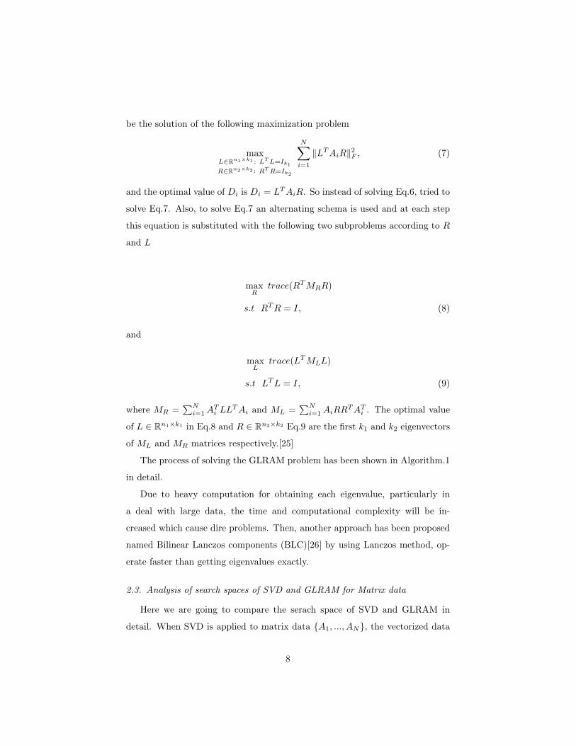
be the solution of the following maximization problem

maxL∈Rn1×k1 : LTL=Ik1

R∈Rn2×k2 : RTR=Ik2

N∑i=1

‖LTAiR‖2F , (7)

and the optimal value of Di is Di = LTAiR. So instead of solving Eq.6, tried to

solve Eq.7. Also, to solve Eq.7 an alternating schema is used and at each step

this equation is substituted with the following two subproblems according to R

and L

maxR

trace(RTMRR)

s.t RTR = I, (8)

and

maxL

trace(LTMLL)

s.t LTL = I, (9)

where MR =∑N

i=1ATi LL

TAi and ML =∑N

i=1AiRRTAT

i . The optimal value

of L ∈ Rn1×k1 in Eq.8 and R ∈ Rn2×k2 Eq.9 are the first k1 and k2 eigenvectors

of ML and MR matrices respectively.[25]

The process of solving the GLRAM problem has been shown in Algorithm.1

in detail.

Due to heavy computation for obtaining each eigenvalue, particularly in

a deal with large data, the time and computational complexity will be in-

creased which cause dire problems. Then, another approach has been proposed

named Bilinear Lanczos components (BLC)[26] by using Lanczos method, op-

erate faster than getting eigenvalues exactly.

2.3. Analysis of search spaces of SVD and GLRAM for Matrix data

Here we are going to compare the serach space of SVD and GLRAM in

detail. When SVD is applied to matrix data {A1, ..., AN}, the vectorized data

8

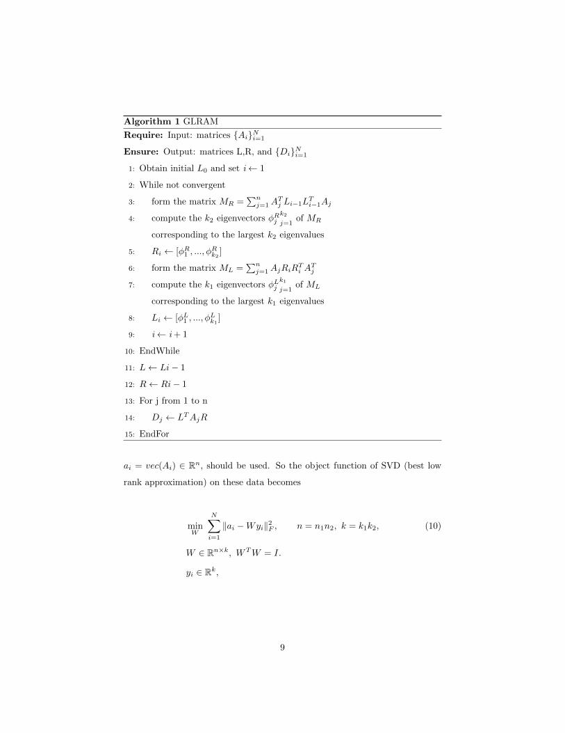
Algorithm 1 GLRAM

Require: Input: matrices {Ai}Ni=1

Ensure: Output: matrices L,R, and {Di}Ni=1

1: Obtain initial L0 and set i← 1

2: While not convergent

3: form the matrix MR =∑n

j=1ATj Li−1L

Ti−1Aj

4: compute the k2 eigenvectors φRjk2

j=1of MR

corresponding to the largest k2 eigenvalues

5: Ri ← [φR1 , ..., φRk2

]

6: form the matrix ML =∑n

j=1AjRiRTi A

Tj

7: compute the k1 eigenvectors φLjk1

j=1of ML

corresponding to the largest k1 eigenvalues

8: Li ← [φL1 , ..., φLk1

]

9: i← i + 1

10: EndWhile

11: L← Li− 1

12: R← Ri− 1

13: For j from 1 to n

14: Dj ← LTAjR

15: EndFor

ai = vec(Ai) ∈ Rn, should be used. So the object function of SVD (best low

rank approximation) on these data becomes

minW

N∑i=1

‖ai −Wyi‖2F , n = n1n2, k = k1k2, (10)

W ∈ Rn×k, WTW = I.

yi ∈ Rk,

9

By using the properties of Kronecker product[29] and vectorization, it is easy

to show that GLRAM model Eq.6, is equal to the following form

minL,R,Di

N∑i=1

‖ai − (L⊗R)di‖2F . (11)

L ∈ Rn1×k1 : LTL = Ik1

R ∈ Rn2×k2 : RTR = Ik2.

Now, by comparison the Eq.10 and Eq.11, we want to describe the relation-

ship between SVD and GLRAM. For every two orthogonal matrices like L and

R in feasible region of Eq.11 their corresponding L⊗R satisfies the constraints

of Eq.10. This means that L ⊗ R is a special case of W in Eq.10. In fact, the

search space of GLRAM is a subset of SVD and it can be considered as a special

case of SVD. By this relationship, the following facts summaries the relationship

of SVD and GLRAM in 3 main parts.

• Far apart the GLRAM works with data in their original format, it is a

special case of SVD.

• GLRAM has n1k1+n2k2 parameters that should be estimated, while there

are n1n2k1k2 ones for SVD. So the GLRAM’s complexity is much less than

SVD and the possibility of overfitting, is too.

• In GLRAM we are free to choose the reduction in each arbitrary mode.

Therefore by the mentioned properties, the GLRAM seems to be better than

SVD (PCA) for matrix data.

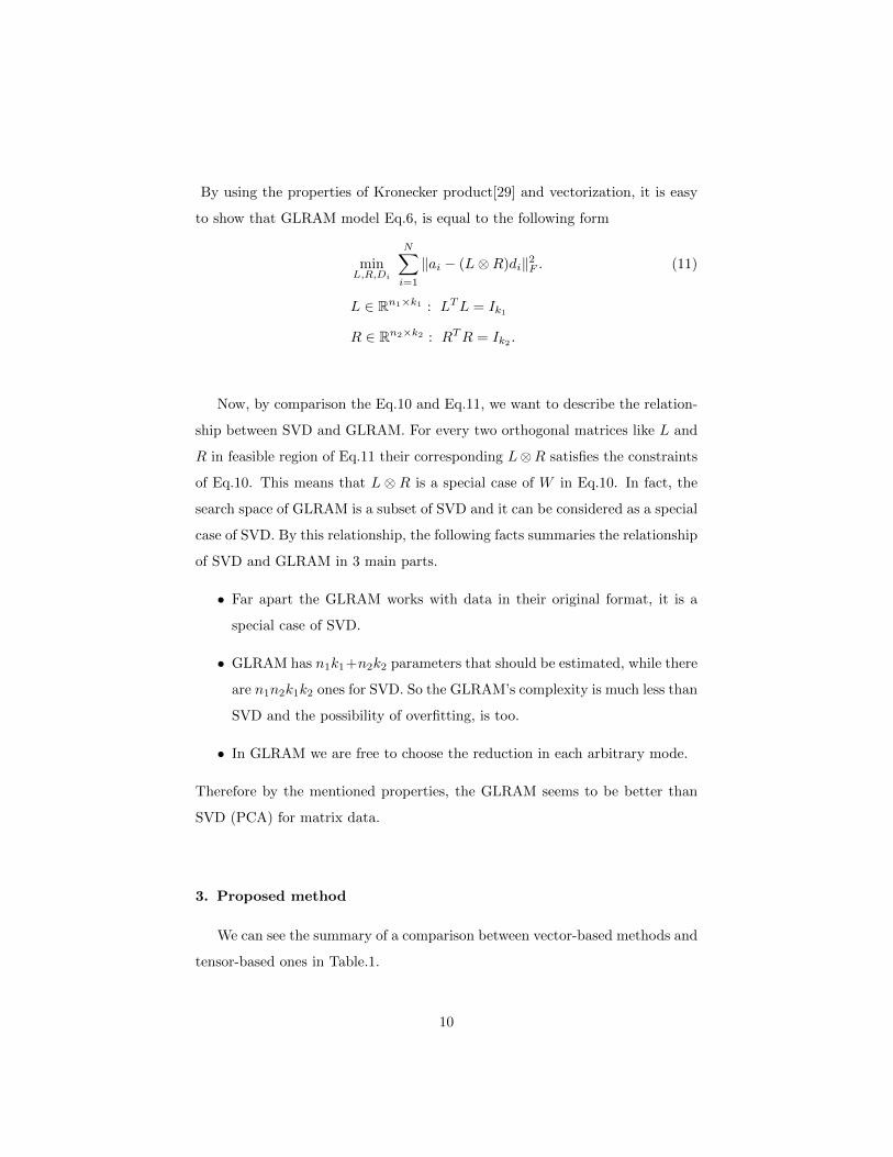
3. Proposed method

We can see the summary of a comparison between vector-based methods and

tensor-based ones in Table.1.

10

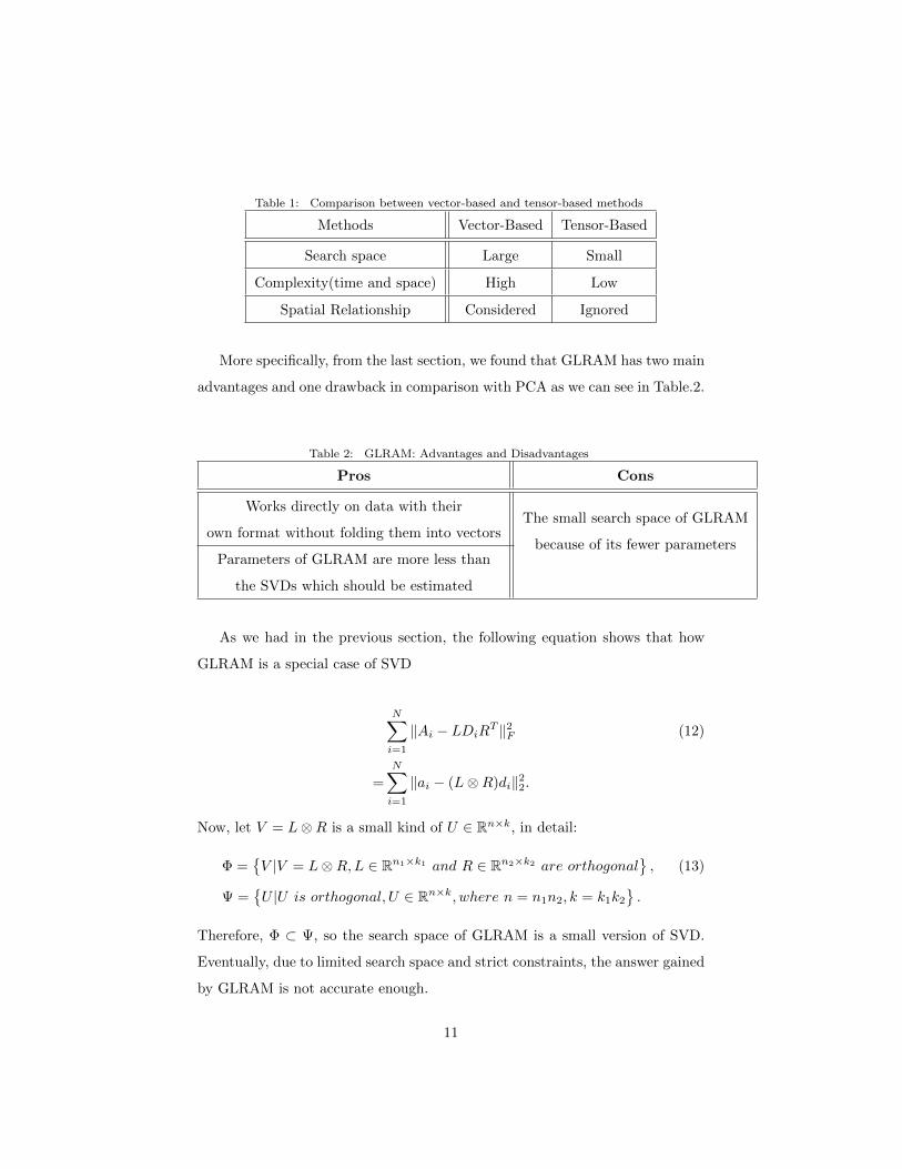
Table 1: Comparison between vector-based and tensor-based methods

Methods Vector-Based Tensor-Based

Search space Large Small

Complexity(time and space) High Low

Spatial Relationship Considered Ignored

More specifically, from the last section, we found that GLRAM has two main

advantages and one drawback in comparison with PCA as we can see in Table.2.

Table 2: GLRAM: Advantages and Disadvantages

Pros Cons

Works directly on data with their

own format without folding them into vectorsThe small search space of GLRAM

because of its fewer parametersParameters of GLRAM are more less than

the SVDs which should be estimated

As we had in the previous section, the following equation shows that how

GLRAM is a special case of SVD

N∑i=1

‖Ai − LDiRT ‖2F (12)

=

N∑i=1

‖ai − (L⊗R)di‖22.

Now, let V = L⊗R is a small kind of U ∈ Rn×k, in detail:

Φ ={V |V = L⊗R,L ∈ Rn1×k1 and R ∈ Rn2×k2 are orthogonal

}, (13)

Ψ ={U |U is orthogonal, U ∈ Rn×k, where n = n1n2, k = k1k2

}.

Therefore, Φ ⊂ Ψ, so the search space of GLRAM is a small version of SVD.

Eventually, due to limited search space and strict constraints, the answer gained

by GLRAM is not accurate enough.

11

In this section, we try to extend the search domain of GLRAM in order to

improve its quality without losing its mentioned advantages shown in Table.2.

To design our proposed method, we should have new insight to search region

Ψ of SVD method. When SVD is used for matrix data samples Ai ∈ Rn1×n2 ,

according to Eq.13, the solution will lie on the feasible set Ψ and each feasible

solution will be an orthogonal matrix U ∈ Rn×k, where n = n1n2 and k = k1k2.

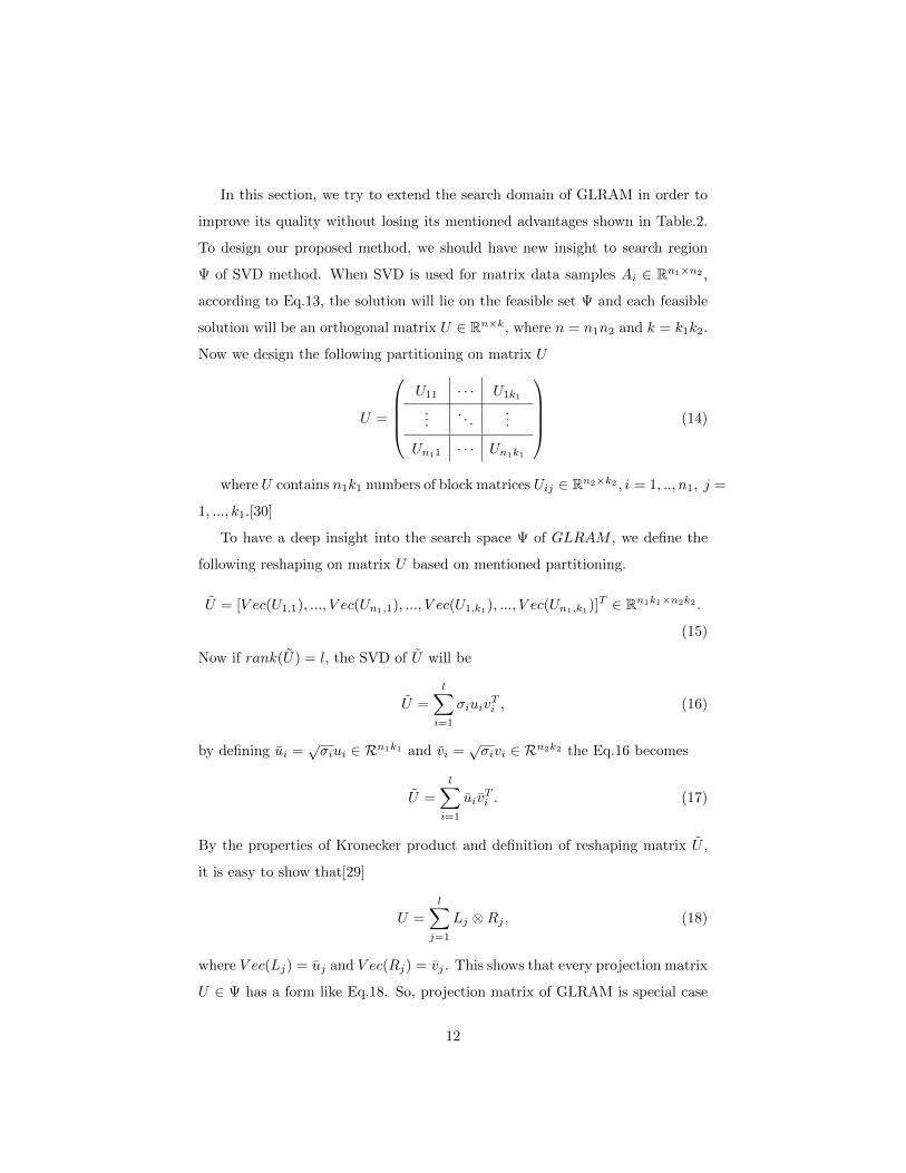
Now we design the following partitioning on matrix U

U =

U11 · · · U1k1

.... . .

...

Un11 · · · Un1k1

(14)

where U contains n1k1 numbers of block matrices Uij ∈ Rn2×k2 , i = 1, .., n1, j =

1, ..., k1.[30]

To have a deep insight into the search space Ψ of GLRAM , we define the

following reshaping on matrix U based on mentioned partitioning.

U = [V ec(U1,1), ..., V ec(Un1,1), ..., V ec(U1,k1), ..., V ec(Un1,k1

)]T ∈ Rn1k1×n2k2 .

(15)

Now if rank(U) = l, the SVD of U will be

U =

l∑i=1

σiuivTi , (16)

by defining ui =√σiui ∈ Rn1k1 and vi =

√σivi ∈ Rn2k2 the Eq.16 becomes

U =

l∑i=1

uivTi . (17)

By the properties of Kronecker product and definition of reshaping matrix U ,

it is easy to show that[29]

U =

l∑j=1

Lj ⊗Rj , (18)

where V ec(Lj) = uj and V ec(Rj) = vj . This shows that every projection matrix

U ∈ Ψ has a form like Eq.18. So, projection matrix of GLRAM is special case

12

of Eq.18 when l = 1.

So, if we set a k larger than 1 and smaller than l, using the projection matrix

like

U =

k∑j=1

Lj ⊗Rj , (19)

enables us to use the benefits of GLRAM and SVD at the same time. This

means that by the mentioned U in Eq.19, as projection matrix in GLRAM

model, we obtained the following approximation model

minLj ,Rj ,Di

N∑i=1

‖ai −k∑

j=1

(Lj ⊗Rj)di‖2F (20)

=

N∑i=1

‖Ai −k∑

j=1

LjDiRTj ‖2F ,

where di = V ec(Di) and Di ∈ Rk1×k2 which similar to GLRAM works on ma-

trix data with their own format and at the same time its search space is larger

than GLRAM method.

So Φk ={∑k

j=1 Lj ⊗Rj |Lj ∈ Rn1×k1 , Rj ∈ Rn2×k2

}denotes the search space

of problem Eq.20 and from Eq.13 we can conclude that Φ ⊂ Φk. Which shows

that by our approach the search space of the problem is increased. Also, from

Eq.20 it is clear that our proposed method is applied to the data with their own

format without folding to vectors. Furthermore, this method has (n1k1+n2k2)k

parameters that should be estimated. Since we consider k as a small number,

so the complexity of this method is not much higher than GLRAM, and still

the probability of occurrence of overfitting is less for this method in comparison

with SVD or PCA.

Although this problem is nonconvex, once it is going to solve according to

each parameter, where other parameters are considered to be known, it will be

a convex one. So we could use coordinate descent approach to deal with it.[31]

13

3.1. Algorithm

In Multiple-Pairs of Generalized Low-Rank Approximation of Matrices (MPGLRAM)

, we deal with the following problem:

minLj∈Rn1×k1 :j=1,2,...,k

Rj∈Rn2×k2 j=1,2,...,k

Di∈Rk1×k2 i=1,2,...N,

N∑i=1

‖Ai −k∑

j=1

LjDiRTj ‖2F . (21)

To solve Eq.21 like GLRAM, we use a coordinate descent[31] approach. So

at each step of the algorithm, we have some subproblems that are solved only

according to one variable. So, after p steps let L(p)j , R

(p)j and D

(p)i are the

estimations of projections and data matrices. At step p + 1 firstly we set the

projection matrices be known as the estimated at step p. Now we have to

estimate the projection matrices with known L(p)j and R

(p)j from the last steps,

which leads to the following subproblem

{D(p+1)i }Ni=1 = arg min

Di,i=1,..,N

N∑i=1

‖Ai −k∑

j=1

L(p)j DiR

(p)T

j ‖2F

= arg mindi,i=1,..,N

N∑i=1

‖ai − (

k∑j=1

R(p)j ⊗ L

(p)j )di‖22 (22)

So, if we set B(p) =∑k

j=1

(R

(p)j ⊗ L

(p)j

), this problem can be reformulated

as the following least squares problem.[32].

minDi=1,..,N

N∑i=1

‖ai −B(p)di‖22 = min ‖A−B(p)D‖2F , ai = vec(Ai), di = vec(Di),

(23)

where A = [a1, ..., aN ] ∈ Rn1n2×N and D = [d1, ..., dN ] ∈ Rk1k2×N . This is

a well-known least square problem and could be solved easily by direct and

iterative matrix computation techniques.

After solving the mentioned problem we should find Lj , Rj parameters

successively by coordinate descent approach for j=1,...,k.[31] So if we assume

14

{Lj , Rj}j=1,...,j′−1,j′+1,...,k are fixed, we should estimate Lj′ and Rj′ in the next

step. By these assumption equation Eq.21, according to Eq.22 and Eq.23 leads

to

minLj ,L

′j∈R

n1×k1 :j=1,2,...,k

Rj ,R′j∈R

n2×k2 :j=1,2,...,k

Di∈Rk1×k2 :i=1,2,...,N

N∑i=1

‖Ai −k∑

j=1j 6=j′

LjDiRTj − Lj′DiR

Tj′‖2F . (24)

By replacing Ai = Ai −k∑

j=1j 6=j′

LjDiRTj the equation becomes

minL′j∈R

n1×k1 :j=1,2,...,k

R′j∈Rn2×k2 :j=1,2,...,k

Di∈Rk1×k2 :i=1,2,...,N

N∑i=1

‖Ai − Lj′DiRTj′‖2F . (25)

For solving Eq.25 we do alternatively. At first, Lj′ , Ai and Di are given.

The only variable should be determined is Rj′ . By replacing Mi = Lj′Di in

Eq.25 and also regarding to Trace properties we have [33]

‖Ai −MiRTj′‖2F = tr

((Ai −MiR

Tj′)

T (Ai −MiRTj′))

= tr(AiTAi − 2Ai

TMiR

Tj′ +Rj′M

Ti MiR

Tj′), (26)

which by removing the constants leads to the following problem

minRj′

N∑i=1

tr(−2AiTMiR

Tj′ +Rj′M

Ti MiR

Tj′)

= minRj′−2

N∑i=1

tr(AiTMiR

Tj′) +

N∑i=1

tr(Rj′MTi MiR

Tj′)

= minRj′−2tr((

N∑i=1

AiTMi)R

Tj′) + tr(Rj′(

N∑i=1

MTi Mi)R

Tj′), (27)

In order to release the dependency of data from the optimization problem, insert

the sigma operators into traces and by replacing NR =∑N

i=1 ATi Mi and BR =∑N

i=1MTi Mi, this optimization problem becomes

minRj′−2tr(NRR

Tj′) + tr(Rj′BRR

Tj′), Rj′ ∈ Rn2×k2 : j = 1, 2, ..., k, (28)

15

Now, for solving Eq.28 since the function of this problem is quadratic convex,

the derivate of this function according to R in the optimal point should be

zero. So by taking, derivative of this objective function with respect to Rj′ ,

and regarding properties of Trace [33], by setting the objective function equal

to zero, we have

−2NR + 2Rj′BR = 0, (29)

and consequently, R′j will be determined.

Rj′ = NRB−1R . (30)

Also, same as obtaining Rj′ we can determine Lj′ with a little difference.

To this purpose, we should solve the transpose of Eq.25 according to Lj′

minLj ,Lj′∈R

n1×k1 :j=1,2,...,k

Rj ,Rj′∈Rn2×k2 :j=1,2,...,k

Di∈Rk1×k2 :i=1,2,...,N

N∑i=1

‖AiT −Rj′D

Ti L

Tj′‖2F . (31)

Let Mi = Rj′DTi ,then

minLj′‖Ai

T −MiLTj′‖2F =tr

((Ai

T −MiLTj′)

T (AiT −MiL

Tj′))

= minLj′

tr(AiAiT − 2AiMiL

Tj′ + Lj′M

Ti MiL

Tj′)

= minLj′−2

N∑i=1

tr((

N∑i=1

AiMi)LTj′) + tr(Lj′(

N∑i=1

MTi Mi)L

Tj′).

(32)

By replacing NL =∑N

i=1 AiMi and BL =∑N

i=1MTi Mi, we have

minLj′−2tr(NLL

Tj′) + tr(Lj′BLL

Tj′). (33)

Then, by taking derivative of this function respect to L′j and after simplification

L′j will be determined.

Lj′ = NLB−1L . (34)

Since we should obtain all k variables, we do previous stages k times to determine

Lj and Rj , for all amount of j = 1, ..., k. Eventually, at each time, k − 1

16

parameters will be assumed fixed to obtain one parameter. And for the next

parameter, the updated form of the previous ones will be used. Besides, we can

repeat this alternative process more than once. Since each time with updating

parameters, the result will be improved. Although, these iterations increase the

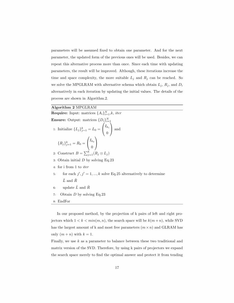
time and space complexity, the more suitable Lj and Rj can be reached. So

we solve the MPGLRAM with alternative schema which obtain Lj , Rj , and Di

alternatively in each iteration by updating the initial values. The details of the

process are shown in Algorithm.2.

Algorithm 2 MPGLRAM

Require: Input: matrices {Ai}Ni=1,k, iter

Ensure: Output: matrices {Di}Ni=1

1: Initialize {Lj}kj=1 = L0 =

Ik1

0

and

{Rj}kj=1 = R0 =

Ik2

0

2: Construct B =

∑kj=1(Rj ⊗ Lj)

3: Obtain initial D by solving Eq.23

4: for i from 1 to iter

5: for each j′, j′ = 1, ..., k solve Eq.25 alternatively to determine

L and R

6: update L and R

7: Obtain D by solving Eq.23

8: EndFor

In our proposed method, by the projection of k pairs of left and right pro-

jectors which 1 < k < min(m,n), the search space will be k(m+n), while SVD

has the largest amount of k and most free parameters (m×n) and GLRAM has

only (m+ n) with k = 1.

Finally, we use k as a parameter to balance between these two traditional and

matrix version of the SVD. Therefore, by using k pairs of projectors we expand

the search space merely to find the optimal answer and protect it from tending

17

to overfitting due to many parameters like SVD.

4. Experimental Results

As we have seen in the previous section, in our proposed method, we ex-

panded the search space of GLRAM problem by using k pair projector matrices

instead of one pair used in GLRAM. Now, we are going to compare MPGLRAM

with GLRAM in 4 datasets in 2 aspects. The first is RMSRE, and the second

is about classification accuracy.

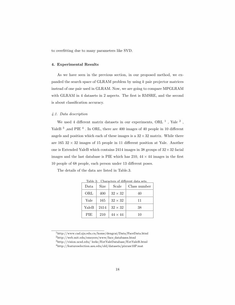
4.1. Data description

We used 4 different matrix datasets in our experiments, ORL 1 , Yale 2 ,

YaleB 3 ,and PIE 4 . In ORL, there are 400 images of 40 people in 10 different

angels and position which each of these images is a 32× 32 matrix. While there

are 165 32 × 32 images of 15 people in 11 different position at Yale. Another

one is Extended YaleB which contains 2414 images in 38 groups of 32×32 facial

images and the last database is PIE which has 210, 44× 44 images in the first

10 people of 68 people, each person under 13 different poses.

The details of the data are listed in Table.3.

Table 3: Characters of different data sets.

Data Size Scale Class number

ORL 400 32× 32 40

Yale 165 32× 32 11

YaleB 2414 32× 32 38

PIE 210 44× 44 10

1http://www.cad.zju.edu.cn/home/dengcai/Data/FaceData.html2http://web.mit.edu/emeyers/www/face databases.html3http://vision.ucsd.edu/ leekc/ExtYaleDatabase/ExtYaleB.html4http://featureselection.asu.edu/old/datasets/pixraw10P.mat

18

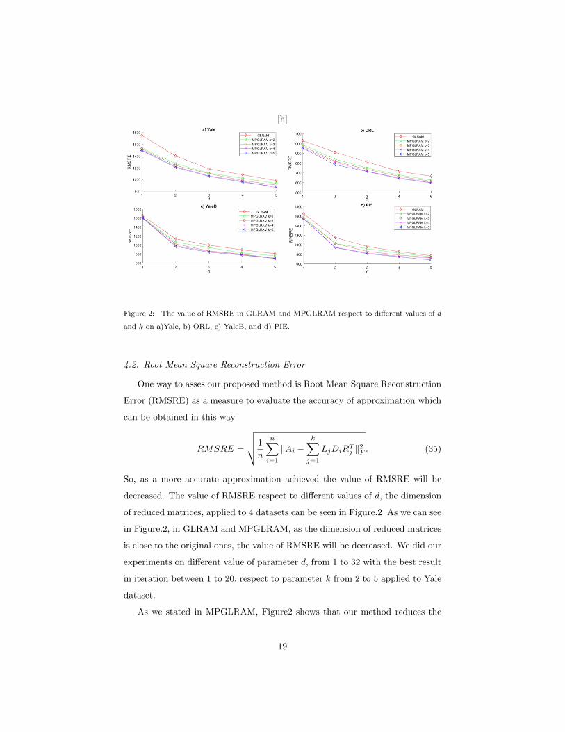
[h]

Figure 2: The value of RMSRE in GLRAM and MPGLRAM respect to different values of d

and k on a)Yale, b) ORL, c) YaleB, and d) PIE.

4.2. Root Mean Square Reconstruction Error

One way to asses our proposed method is Root Mean Square Reconstruction

Error (RMSRE) as a measure to evaluate the accuracy of approximation which

can be obtained in this way

RMSRE =

√√√√ 1

n

n∑i=1

‖Ai −k∑

j=1

LjDiRTj ‖2F . (35)

So, as a more accurate approximation achieved the value of RMSRE will be

decreased. The value of RMSRE respect to different values of d, the dimension

of reduced matrices, applied to 4 datasets can be seen in Figure.2 As we can see

in Figure.2, in GLRAM and MPGLRAM, as the dimension of reduced matrices

is close to the original ones, the value of RMSRE will be decreased. We did our

experiments on different value of parameter d, from 1 to 32 with the best result

in iteration between 1 to 20, respect to parameter k from 2 to 5 applied to Yale

dataset.

As we stated in MPGLRAM, Figure2 shows that our method reduces the

19

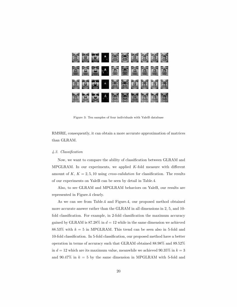
Figure 3: Ten samples of four individuals with YaleB database

RMSRE, consequently, it can obtain a more accurate approximation of matrices

than GLRAM.

4.3. Classification

Now, we want to compare the ability of classification between GLRAM and

MPGLRAM. In our experiments, we applied K-fold measure with different

amount of K, K = 2, 5, 10 using cross-validation for classification. The results

of our experiments on YaleB can be seen by detail in Table.4.

Also, to see GLRAM and MPGLRAM behaviors on YaleB, our results are

represented in Figure.4 clearly.

As we can see from Table.4 and Figure.4, our proposed method obtained

more accurate answer rather than the GLRAM in all dimensions in 2, 5, and 10-

fold classification. For example, in 2-fold classification the maximum accuracy

gained by GLRAM is 87.28% in d = 12 while in the same dimension we achieved

88.53% with k = 5 in MPGLRAM. This trend can be seen also in 5-fold and

10-fold classification. In 5-fold classification, our proposed method have a better

operation in terms of accuracy such that GLRAM obtained 88.98% and 89.52%

in d = 12 which are its maximum value, meanwhile we achieved 90.35% in k = 3

and 90.47% in k = 5 by the same dimension in MPGLRAM with 5-fold and

20

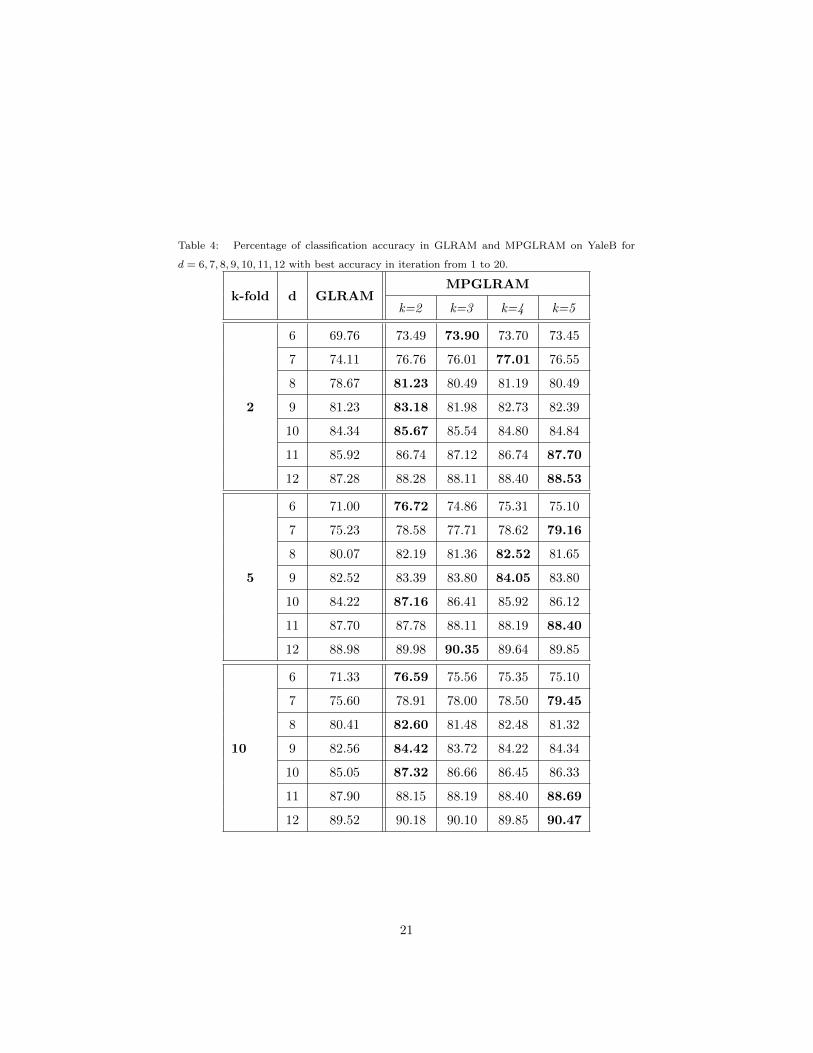
Table 4: Percentage of classification accuracy in GLRAM and MPGLRAM on YaleB for

d = 6, 7, 8, 9, 10, 11, 12 with best accuracy in iteration from 1 to 20.

k-fold d GLRAMMPGLRAM

k=2 k=3 k=4 k=5

2

6 69.76 73.49 73.90 73.70 73.45

7 74.11 76.76 76.01 77.01 76.55

8 78.67 81.23 80.49 81.19 80.49

9 81.23 83.18 81.98 82.73 82.39

10 84.34 85.67 85.54 84.80 84.84

11 85.92 86.74 87.12 86.74 87.70

12 87.28 88.28 88.11 88.40 88.53

5

6 71.00 76.72 74.86 75.31 75.10

7 75.23 78.58 77.71 78.62 79.16

8 80.07 82.19 81.36 82.52 81.65

9 82.52 83.39 83.80 84.05 83.80

10 84.22 87.16 86.41 85.92 86.12

11 87.70 87.78 88.11 88.19 88.40

12 88.98 89.98 90.35 89.64 89.85

10

6 71.33 76.59 75.56 75.35 75.10

7 75.60 78.91 78.00 78.50 79.45

8 80.41 82.60 81.48 82.48 81.32

9 82.56 84.42 83.72 84.22 84.34

10 85.05 87.32 86.66 86.45 86.33

11 87.90 88.15 88.19 88.40 88.69

12 89.52 90.18 90.10 89.85 90.47

21

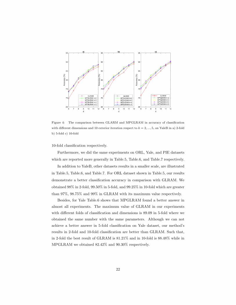
Figure 4: The comparison between GLARM and MPGLRAM in accuracy of classification

with different dimensions and 10 exterior iteration respect to k = 2, ..., 5, on YaleB in a) 2-fold

b) 5-fold c) 10-fold

10-fold classification respectively.

Furthermore, we did the same experiments on ORL, Yale, and PIE datasets

which are reported more generally in Table.5, Table.6, and Table.7 respectively.

In addition to YaleB, other datasets results in a smaller scale, are illustrated

in Table.5, Table.6, and Table.7. For ORL dataset shown in Table.5, our results

demonstrate a better classification accuracy in comparison with GLRAM. We

obtained 98% in 2-fold, 99.50% in 5-fold, and 99.25% in 10-fold which are greater

than 97%, 98.75% and 99% in GLRAM with its maximum value respectively.

Besides, for Yale Table.6 shows that MPGLRAM found a better answer in

almost all experiments. The maximum value of GLRAM in our experiments

with different folds of classification and dimensions is 89.09 in 5-fold where we

obtained the same number with the same parameters. Although we can not

achieve a better answer in 5-fold classification on Yale dataset, our method’s

results in 2-fold and 10-fold classification are better than GLRAM. Such that,

in 2-fold the best result of GLRAM is 81.21% and in 10-fold is 88.48% while in

MPGLRAM we obtained 82.42% and 90.30% respectively.

22

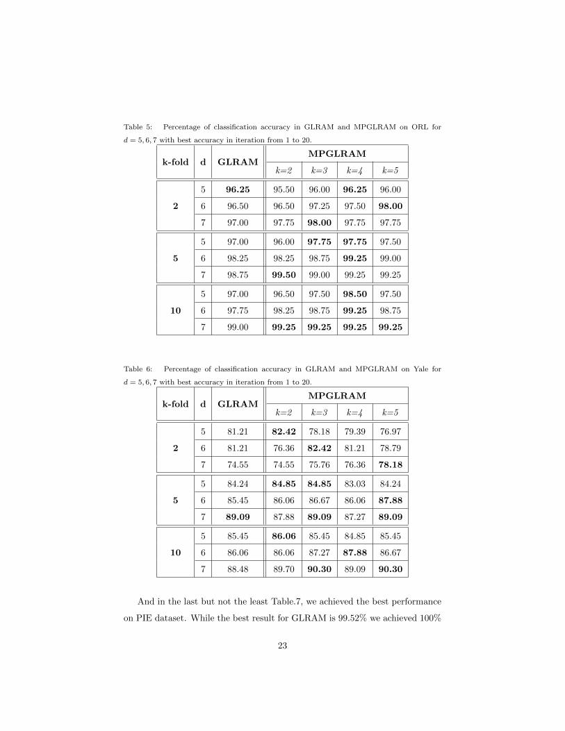
Table 5: Percentage of classification accuracy in GLRAM and MPGLRAM on ORL for

d = 5, 6, 7 with best accuracy in iteration from 1 to 20.

k-fold d GLRAMMPGLRAM

k=2 k=3 k=4 k=5

2

5 96.25 95.50 96.00 96.25 96.00

6 96.50 96.50 97.25 97.50 98.00

7 97.00 97.75 98.00 97.75 97.75

5

5 97.00 96.00 97.75 97.75 97.50

6 98.25 98.25 98.75 99.25 99.00

7 98.75 99.50 99.00 99.25 99.25

10

5 97.00 96.50 97.50 98.50 97.50

6 97.75 98.25 98.75 99.25 98.75

7 99.00 99.25 99.25 99.25 99.25

Table 6: Percentage of classification accuracy in GLRAM and MPGLRAM on Yale for

d = 5, 6, 7 with best accuracy in iteration from 1 to 20.

k-fold d GLRAMMPGLRAM

k=2 k=3 k=4 k=5

2

5 81.21 82.42 78.18 79.39 76.97

6 81.21 76.36 82.42 81.21 78.79

7 74.55 74.55 75.76 76.36 78.18

5

5 84.24 84.85 84.85 83.03 84.24

6 85.45 86.06 86.67 86.06 87.88

7 89.09 87.88 89.09 87.27 89.09

10

5 85.45 86.06 85.45 84.85 85.45

6 86.06 86.06 87.27 87.88 86.67

7 88.48 89.70 90.30 89.09 90.30

And in the last but not the least Table.7, we achieved the best performance

on PIE dataset. While the best result for GLRAM is 99.52% we achieved 100%

23

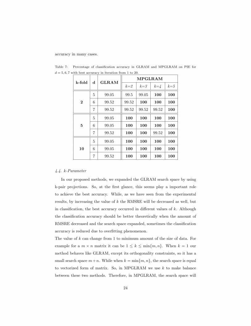
accuracy in many cases.

Table 7: Percentage of classification accuracy in GLRAM and MPGLRAM on PIE for

d = 5, 6, 7 with best accuracy in iteration from 1 to 20.

k-fold d GLRAMMPGLRAM

k=2 k=3 k=4 k=5

2

5 99.05 99.5 99.05 100 100

6 99.52 99.52 100 100 100

7 99.52 99.52 99.52 99.52 100

5

5 99.05 100 100 100 100

6 99.05 100 100 100 100

7 99.52 100 100 99.52 100

10

5 99.05 100 100 100 100

6 99.05 100 100 100 100

7 99.52 100 100 100 100

4.4. k-Parameter

In our proposed methods, we expanded the GLRAM search space by using

k-pair projections. So, at the first glance, this seems play a important role

to achieve the best accuracy. While, as we have seen from the experimental

results, by increasing the value of k the RMSRE will be decreased as well, but

in classification, the best accuracy occurred in different values of k. Although

the classification accuracy should be better theoretically when the amount of

RMSRE decreased and the search space expanded, sometimes the classification

accuracy is reduced due to overfitting phenomenon.

The value of k can change from 1 to minimum amount of the size of data. For

example for a m × n matrix it can be 1 ≤ k ≤ min{m,n}. When k = 1 our

method behaves like GLRAM, except its orthogonality constraints, so it has a

small search space m+n. While when k = min{m,n}, the search space is equal

to vectorized form of matrix. So, in MPGLRAM we use k to make balance

between these two methods. Therefore, in MPGLRAM, the search space will

24

be k(m + n) which can be larger than GLRAM and smaller than vectorized

dimension reduction method, SVD.

In our experiments we use k = 2, 3, 4, 5 to show that the proposed method works

better than GLRAM especially when the dimension reduced to a lower value.

5. Conclusion

In this paper we proposed a new method using advantages of both SVD and

GLRAM simultaneously to find a more accurate answer rather than GLRAM

with lower complexity than SVD. Then, since GLRAM has few parameters and

the search space of it is too small to finding an optimal answer, we proposed an

approach that try to expand the search space of GLRAM in order to find a more

accurate answer. For this purpose, we used k-pair projection matrices instead

of one pair in GLRAM. Therefore by increasing the parameters and making a

larger search space, the probability of finding optimal answer will be increased.

Many experimental results have been represented in section.4 to illustrate that

our proposed method, MPGLRAM, works better than GLRAM in terms of less

RMSRE and therefore, more classification accuracy.

References

References

[1] Zhao W, Chellappa R, Phillips PJ, Rosenfeld A. Face recognition: A liter-

ature survey. ACM computing surveys (CSUR). 2003 Dec 1;35(4):399-458.

[2] Umbaugh SE. Digital image processing and analysis: human and computer

vision applications with CVIPtools. CRC press; 2016 Apr 19.

[3] Jordan MI, Mitchell TM. Machine learning: Trends, perspectives, and

prospects. Science. 2015 Jul 17;349(6245):255-60.

[4] Wernick MN, Yang Y, Brankov JG, Yourganov G, Strother SC. Ma-

chine learning in medical imaging. IEEE signal processing magazine. 2010

Jul;27(4):25-38.

25

[5] Brunetti A, Buongiorno D, Trotta GF, Bevilacqua V. Computer vision and

deep learning techniques for pedestrian detection and tracking: A survey.

Neurocomputing. 2018 Jul 26;300:17-33.

[6] Vadim K. Overview of different approaches to solving problems of Data

Mining. Procedia Computer Science. 2018 Dec 31;123:234-9.

[7] Hearst MA, Dumais ST, Osuna E, Platt J, Scholkopf B. Support vector ma-

chines. IEEE Intelligent Systems and their applications. 1998 Jul;13(4):18-

28.

[8] Ye J, Li Q. LDA/QR: an efficient and effective dimension reduction al-

gorithm and its theoretical foundation. Pattern recognition. 2004 Apr

1;37(4):851-4.

[9] Christopher MB. PATTERN RECOGNITION AND MACHINE LEARN-

ING. Springer-Verlag New York; 2016.

[10] Klema V, Laub A. The singular value decomposition: Its computation

and some applications. IEEE Transactions on automatic control. 1980

Apr;25(2):164-76.

[11] Cai D, He X, Hu Y, Han J, Huang T. Learning a spatially smooth subspace

for face recognition. InComputer Vision and Pattern Recognition, 2007.

CVPR’07. IEEE Conference on 2007 Jun 17 (pp. 1-7). IEEE.

[12] Lu H, Plataniotis KN, Venetsanopoulos AN. A survey of multilinear sub-

space learning for tensor data. Pattern Recognition. 2011 Jul 1;44(7):1540-

51.

[13] Kolda TG, Bader BW. Tensor decompositions and applications. SIAM re-

view. 2009 Aug 5;51(3):455-500.

[14] Donoho DL. High-dimensional data analysis: The curses and blessings of

dimensionality. AMS Math Challenges Lecture. 2000 Aug 6;1:32.

26

[15] Lu H, Plataniotis KN, Venetsanopoulos AN. MPCA: Multilinear principal

component analysis of tensor objects. IEEE transactions on Neural Net-

works. 2008 Jan;19(1):18-39.

[16] Lu H, Plataniotis KN, Venetsanopoulos AN. A taxonomy of emerging mul-

tilinear discriminant analysis solutions for biometric signal recognition. Wi-

ley/IEEE; 2009 Oct 29.

[17] Guo X, Huang X, Zhang L, Zhang L, Plaza A, Benediktsson JA. Sup-

port tensor machines for classification of hyperspectral remote sensing

imagery. IEEE Transactions on Geoscience and Remote Sensing. 2016

Jun;54(6):3248-64.

[18] Nie F, Xiang S, Song Y, Zhang C. Extracting the optimal dimensional-

ity for local tensor discriminant analysis. Pattern Recognition. 2009 Jan

1;42(1):105-14.

[19] Tao D, Li X, Hu W, Maybank S, Wu X. Supervised tensor learning. In

Data Mining, Fifth IEEE International Conference on 2005 Nov 27 (pp.

8-pp). IEEE.

[20] Dong W, Wang P, Yin W, Shi G, Wu F, Lu X. Denoising Prior Driven Deep

Neural Network for Image Restoration. arXiv preprint arXiv:1801.06756.

2018 Jan 21.

[21] Ghaddar A, Razafindralambo T, Simplot-Ryl I, Tawbi S, Hijazi A. Al-

gorithm for data similarity measurements to reduce data redundancy in

wireless sensor networks. InWorld of Wireless Mobile and Multimedia Net-

works (WoWMoM), 2010 IEEE International Symposium on a 2010 Jun 14

(pp. 1-6). IEEE.

[22] Wiatowski T, Blcskei H. A mathematical theory of deep convolutional neu-

ral networks for feature extraction. IEEE Transactions on Information The-

ory. 2018 Mar;64(3):1845-66.

27

[23] Van Der Maaten L, Postma E, Van den Herik J. Dimensionality reduction:

a comparative. J Mach Learn Res. 2009 Oct 26;10:66-71.

[24] Bjrck . Numerical methods in matrix computations. Springer; 2016.

[25] Ye J. Generalized low rank approximations of matrices. Machine Learning.

2005 Nov 1;61(1-3):167-91.

[26] Ren CX, Dai DQ. Bilinear Lanczos components for fast dimension-

ality reduction and feature extraction. Pattern recognition. 2010 Nov

1;43(11):3742-52.

[27] Hou C, Nie F, Zhang C, Yi D, Wu Y. Multiple rank multi-linear SVM for

matrix data classification. Pattern Recognition. 2014 Jan 1;47(1):454-69.

[28] Jimenez LO, Landgrebe DA. Supervised classification in high-dimensional

space: geometrical, statistical, and asymptotical properties of multivari-

ate data. IEEE Transactions on Systems, Man, and Cybernetics, Part C

(Applications and Reviews). 1998 Feb;28(1):39-54.

[29] Van Loan CF, Pitsianis N. Approximation with Kronecker products. In

Linear algebra for large scale and real-time applications 1993 (pp. 293-314).

Springer, Dordrecht.

[30] Rezghi M, Hosseini SM, Elden L. Best Kronecker product approxima-

tion of the blurring operator in three dimensional image restoration prob-

lems. SIAM Journal on Matrix Analysis and Applications. 2014 Aug

19;35(3):1086-104.

[31] Wang X, Zhang W, Yan J, Yuan X, Zha H. On the flexibility of block

coordinate descent for large-scale optimization. Neurocomputing. 2018 Jan

10;272:471-80.

[32] Lawson CL, Hanson RJ. Solving least squares problems. Siam; 1995 Dec 1.

[33] Petersen KB, Pedersen MS. The Matrix Cookbook, Version: November 15.

28