1

Low-rank Matrix Approximation UsingPoint-wise Operators

Arash Amini, Amin Karbasi, Student Member, IEEE, Farokh Marvasti, Senior, IEEE,and Martin Vetterli, Fellow, IEEE,

Abstract—The problem of extracting low dimensional structurefrom high dimensional data arises in many applications such asmachine learning, statistical pattern recognition, wireless sensornetworks, and data compression. If the data is restricted to alower dimensional subspace, then simple algorithms using linearprojections can find the subspace and consequently estimate itsdimensionality. However, if the data lies on a low dimensionalbut nonlinear space (e.g., manifolds), then its structure may behighly nonlinear and hence linear methods are doomed to fail.In this paper we introduce a new technique for dimensionality

reduction based on point-wise operators. More precisely, letAn!n be a matrix of rank k ! n and assume that the matrixBn!n is generated by taking the elements of A to some realpower p. In this paper we show that based on the values ofthe data matrix B, one can estimate the value p and therefore,the underlying low-rank matrix A; i.e., we are reducing thedimensionality of B by using point-wise operators. Moreover,the estimation algorithm does not need to know the rank of A.We also provide bounds on the quality of the approximation andvalidate the stability of the proposed algorithm with simulationsin noisy environments.

Index Terms—Dimensionality Reduction, Low-Rank Matrix,Point-wise Operator.

I. INTRODUCTION

A fundamental question regarding the real-world data isthe degrees of freedom involved in their generation. The termintrinsic dimension, which is the main focus of dimensionalityreduction methods, refers to the number of independent vari-ables for describing a model or a class of signals. Investigationof the intrinsic dimension arises in a variety of settings such asmachine learning [1], computer vision [2], sensor networks [3],bandwidth compression [4], and compressed learning [5].The purpose of reducing the dimension is to obtain a morecompact representation of the data with no or little loss ofinformation. Simplification of the data structure enables us touse the traditional machinery provided for low dimensionaldata, whereas oversimplifying, results in the loss of crucialinformation. Hence, there has been significant interest overthe last few decades in finding dimensionality reductions thatpreserve as much information as possible.

A. Amini and F. Marvasti are with the Advanced Communication ResearchInstitute (ACRI), EE department, Sharif University of Technology, Tehran,Iran. E-mail: arashsil@ee.sharif.edu, marvasti@sharif.edu.A. Karbasi and M. Vetterli are with the School of Computer and Com-

munication Sciences, Ecole Polytechnique Federale de Lausanne (EPFL),Lausanne, Switzerland. Email: {amin.karbasi, martin.vetterli}@epfl.ch.Manuscript received November 27, 2010; revised July 13, 2011.The first author is supported by the Iranian Telecommunication Research

Center (ITRC) in part.

One way to formalize this problem is by representing thedata as a matrix B and then find a low-rank matrix A thatwell approximates B. The main intuition behind this methodis that the rank of a matrix roughly represents its degrees offreedom.It is known that the best low-rank approximation (in terms

of the Frobenius norm) of B is given by the truncated singularvalue decomposition (SVD). More precisely, let Bk denote thematrix obtained by keeping the k largest singular values of Band setting the rest to zero. Then one can show that for allMfor which rank(M) = k,

!B"Bk!F # !M"B!F ,

where ! · !F denotes the Frobenius norm. This approach isshown to be successful in a variety of areas such as informationretrieval [6], face recognition [2] and matrix completion [7],[8] where the matrix B is approximately low-rank.In this paper we look at dimensionality reduction from

the signal processing point of view. More specifically, inapplications such as wireless sensor networks and ultrasoundtomography, where the system contains a number of separatednodes and the communication channel distorts the transmittedsignals among the nodes. In many cases, if the matrix Amodels the transmitted (ideal) signals from each node to therest of the network, A is low-rank due to the structure ofthe network and the type of the transmitted signals. Now, thecorresponding matrix of the received signals, B, is formedfrom A through point-wise but nonlinear operations. Hence,the linear approximation of B will no longer lead to a faithfulrepresentation of the data, while finding the inverse operatorwill do the job. Thus, the fundamental question is how to findthis inverse operator which leads to the approximation of thedesired low-rank matrix.To illustrate this point, below we will describe two appli-

cations as typical examples.

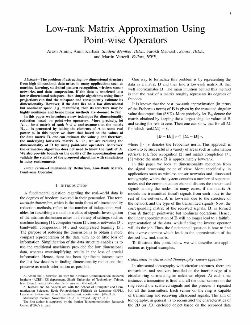
Calibration in Ultrasound Tomography: known operatorIn ultrasound tomography with circular apertures, there are

transmitters and receivers installed on the interior edge of acircular ring surrounding an unknown object. At each timeinstance, a transmitter is fired and all the other sensors on thering record the scattered signals and the process is repeatedfor all the transmitters. Each sensor on the ring is capableof transmitting and receiving ultrasound signals. The aim oftomography, in general, is to reconstruct the characteristics ofthe 2D (or 3D) enclosed object based on the recorded data

2

Fig. 1. Circular setup for ultrasound tomography. Sensors are fired each inturn and the remaining sensors record the arriving ultrasound signals.

(e.g. sound speed, sound attenuation, etc.). The general setupfor such a tomography device is depicted in Fig. I.Before the start of the recording process, the apparatus

should be calibrated. To this end, the relative time of flightsbetween each transmitter-receiver pair are measured. Moreformally, let tij denote the flight time between transmitter iand receiver j and let T denote the matrix of flight timesgiven by T = [tij ]n!n. Because of the circular placementof the sensors, it is easy to check that only a small fractionof the total

!n2

"flight times suffices to estimate the rest;

i.e., the intrinsic dimension is much less than the nominaldimension. In general, T is a full-rank matrix, however, thematrix T = [t2i,j ]n!n is shown to have rank 3 [9]. Therefore,the linear projection of T onto the rank 3 matrices will provideus with a much better calibration result than the receivedmatrix T.This is a situation where both the intrinsic dimension (rank=3)and the point-wise operator (x2) are known a priori. The samephenomenon also happens in the Time of Arrival estimation(TOA) of a sound source when a series of microphones isdeployed [10].

Sensor LocalizationIn radio communications, the received signal power de-

creases as the distance between the transmitter and the receiverincreases; this phenomenon is called path-loss. In general,the received signal power from a transmitter at distance r isproportional to:

1

r!

where the exponent ! varies between 2 in free space to 6 inheavily built urban areas [11].In a sensor localization problem, n sensor nodes are located

in a d-dimensional space where each sensor measures itsdistance to other (probably neighboring) sensors. In practice,exact distance measurements are not directly available andmust be estimated using the Received Signal Strength (RSS).More formally, let dij denote the Euclidean distance betweenthe nodes i and j, and let D denote the distance matrix givenby D = [di,j ]n!n. Furthermore, let pij denote the receivedsignal power by sensor i from sensor j and let P = [p i,j ]n!n.

Given the pairwise distances, the positions of the sensorscan be found using MultiDimensional Scaling (MDS) [12].Unfortunately, in practice the matrix D is not available andshould be estimated through P. Although the matrix P is full-rank in general, it is not difficult to see that its point-wisetransformed matrix P = [p"2!

i,j ]n!n has a rank not exceedingd+2. Therefore, estimating the matrix P will provide us witha low-rank matrix that can later be used for many kinds ofsensor localization algorithms [9], [13].Since ! is a property of the environment, it is usually

unknown. Hence, we are in a situation where the intrinsicdimension is known (d+2) but the point-wise operator linkingthe high rank matrix to the low-rank one is unknown (x"2!).In this work, we consider this problem in its general form,

namely, two matrices, one low-rank and the other full-rank (orwith a higher rank than the first one) that are linked througha polynomial point-wise operator. Given the full-rank matrix,we would like to obtain the low-rank one without a prioriknowledge of the rank or the point-wise operator.

Related workTruncated singular value decomposition became popular by

the pioneer work of Papadimitriou et al. [14] who proved thatlatent semantic analysis works under the context of a simpli-fied model. This method generates faithful low dimensionalrepresentations when the high dimensional input patterns aremainly confined to a low dimensional subspace.The nuclear norm of a Matrix is defined as the sum of

the singular values. For a partially known matrix (e.g., weknow some of the entries or their linear combinations) it isshown in [15] that by constraint nuclear norm minimization wecan achieve the matrix with the minimum rank satisfying theconstraints. This can be interpreted as the matrix form of thecompressed sensing where low rank matrices are considered asthe 2D generalization of sparse vectors and "1-norm minimiza-tion is replaced with nuclear norm minimization[16]. Besidethe nuclear norm, there are other minimization problems suchas log-det penalty function which heuristically lead to thematrix with the minimum rank [17], [18].Graph-based methods have recently received some attention

as a powerful tool for analyzing high dimensional data whichis sampled from a low dimensional sub-manifold. Thesemethods begin by constructing a sparse graph in which nodesrepresent input patterns and edges represent neighborhoodrelations. The resulting graph can be viewed as a discretizedapproximation of the sub-manifold sampled by the inputpatterns. From these graphs, one can then construct matriceswhose spectral decompositions reveal the low dimensionalstructure of the sub-manifold (and sometimes even the dimen-sionality itself). A detailed survey of many of these algorithmsis given in [19]. These algorithms find the low dimensionalembedding using the properties of the manifold. Isomap [20]is based on computing the low dimensional representation ofa high dimensional data set that most faithfully preserves thepairwise distances between input patterns as measured alongthe sub-manifold from which they were sampled. Maximumvariance unfolding [21] tries to maintain the distances and

3

angles between nearby input patterns. The main goal in locallylinear embedding is to keep the local linear structure of nearbyinput patterns [22]. Finally, Laplacian eigenmaps map nearbyinput patterns to the nearby outputs by preserving proximityrelations [23].In the context of bandwidth reduction, the point-wise op-

erators of the form xp for p $ N are previously studied in[4]. In fact, the point-wise operator xp extends the bandwidthof a lowpass signal; based on the root-multiplicities of thederivative of a bandlimited signal, it is shown in [4] thatone can estimate integer ps and therefore, reduce the effectivebandwidth.Our approach differs significantly from the previous works.

Our work is closer to the recent work [24] on compressedsensing where the authors consider two correlated signalslinked by a sparse filter.The rest of this paper is organized as follows. In Sec. II, we

introduce formally the problem and state the main results inSec. III. Section IV provides simulation and numerical resultsand Sec. V concludes the paper.

II. NOTATIONS AND STATEMENT OF THE PROBLEMWe begin by definitions and notations which are used

throughout the paper.

NotationsThese notations are consistently used throughout the paper:

we use % to indicate an element-wise operation on a matrixor a vector; for instance, if A = [ai,j ]m!n then A#2 =#a2i,j

$m!n

and %f(A) =#f(ai,j)

$m!n

. The rank-deficientmatrix and its rank are represented by A and k, respectively,and if B = %f(A), f(.) is called the distorting operatorrelating B to A. Furthermore, the inverse of f(.) (if exists)is called the rank minimizing operator. We also represent thenoisy version of B by B.Since we frequently use the determinant of some specific

matrices, we define the following notations:

TB(x) = det!B#x

", (1)

TB(q1, . . . , qn) = det%#

(ln bi,j)qi$&

. (2)

In this paper, Z and Z+ denote the set of integers and non-negative integers (zero included), respectively.Problem statement: Let f(x) = xp be the polynomial

distortion function with unknown but fixed p > 0. Moreover,let f(x) link the rank deficient square matrix A to the squarematrix B as follows:

B = %f(A) =#f(ai,j)

$.

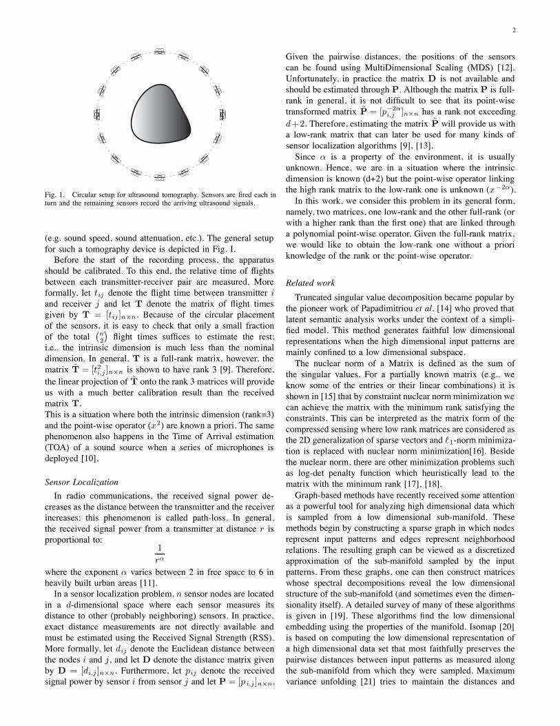
The goal is to estimate the point-wise operator f(x) andconsequently the rank deficient matrix A given the matrix B(see Figure 2).

III. MAIN RESULTSIn this section, we explain our results regarding the men-

tioned problem in form of lemmas and theorems.

f(x)

Low rank High Rank

Fig. 2. The distortion function linking matrix A to B.

A. Monomials with Integer-Valued PowerThe following theorem reveals the effect of polynomial-type

distorting functions on a rank-deficient matrix:Theorem 1: Let An!n be a matrix of rank k and p be an

arbitrary positive integer, we have:

rank!A#p

"# min

'n,

(k + p" 1

p

)*. (3)

Proof Since rank(A) = k, we can select k linearlyindependent row vectors {vi}ki=1 among the rows of A.This means that the rows of A can be written as the linearcombination of these vectors:

An!n =

+

,-c1,1 . . . c1,k...

. . ....

cn,1 . . . cn,k

.

/0

1 23 4Cn!k

+

,-v1...vk

.

/0

1 23 4Vk!n

=56k

l=1 ci,lvl,j7. (4)

Therefore, we have:

A#p =

8! k9

l=1

ci,lvl,j"p:

=

8 9

p1+···+pk=ppi$Z+

(p

p1, . . . , pk

) k;

l=1

(ci,lvl,j)pl

:

=9

p1+···+pk=ppi$Z+

(p

p1, . . . , pk

)8 k;

l=1

(ci,lvl,j)pl

:, (5)

where#<k

l=1(ci,lvl,j)pl$stands for the n&n matrix for which<k

l=1(ci,lvl,j)pl is the i, j element and Z+ represents the set

of non-negative integers. Thus:

rank(A#p) #9

p1+···+pk=ppi$Z+

rank(8 k;

l=1

(ci,lvl,j)pl

:). (6)

Note that:

# k;

l=1

(ci,lvl,j)pl$=

+

,,-

<kl=1 c

pl

1,l...<k

l=1 cpl

n,l

.

//05<k

l=1 vpl

l,1 . . .<k

l=1 vpl

l,n

7, (7)

4

which suggests

rank(8 k;

l=1

(ci,lvl,j)pl

:)= 1. (8)

Combining this result with (6), we get:

rank(A#p) #9

p1+···+pk=ppi$Z+

1 =

(k + p" 1

p

), (9)

and the proof is complete. !Remark 1: If A is a circulant matrix such that the first row

has only k non-zero and consecutive DFT coefficients,

rank(A#p) # p(k " 1) + 1. (10)

According to the properties of the Fourier series, if a,b, care vectors of the same size such that a = b % c, the DFTcoefficients of a are obtained by circularly convolving theDFT coefficients of b, c. In addition, we know that circulantmatrices can be diagonally decomposed using DFT and IDFTunitary matrices where the diagonal matrix contains the DFTcoefficients of the first row on its main diagonal (eigen-values).This suggests that the eigen-values of A#p are found by p-fold circular convolution of the DFT coefficients of the firstrow of A which results in (10).Remark 2: The distorting operator in Theorem 1 can be

considered as a special case of the polynomial operator withB = %f(A) where f(x) =

6pi=0 fix

i; in fact, f(x) is amonic monomial in Theorem 1. For the general polynomialoperator, we have:

%f(A) =p9

i=0

fiA#i, (11)

thus

rank!% f(A)

"#

p9

i=0

rank!A#i

"

#p9

i=0

(k + i" 1

i

)=

(k + p

p

). (12)

Remark 3: The bound in Theorem 1 is often achieved.This is helpful for detecting polynomially distorted low-rankmatrices: assume f(x) is a polynomial of degree p and An!n

is a matrix of rank kA where kA is small compared to n.Moreover, let B = %f(A) be the distorted version with rankkB #

!kA+pp

". If B is a general rank-deficient matrix of

rank kB, the matrix B#i (i $ N) will most likely have therank

!kB+i"1i

". However, B#i can be related to A using a

polynomial of degree p+ i which implies that the rank of thismatrix is upper-bounded by

!kA+p+i

p+i

". It is not hard to check

that the latter upper-bound is less than the general upper-bound!kB+i"1

i

"; this fact, simply distinguishes B from a general

rank-deficient matrix subject to the condition that kA is smallenough compared to n, otherwise,B#i or evenB are probablyfull-rank matrices. Furthermore, the trend of rank

!B#i

"with

respect to i can reveal the degree of the distorting polynomial

(f ): if rank!A#i

"'

!kA+i

i

", then rank

!B"i+1

"

rank!B"i

" ' 1+ kAp+i+1

for a range of i values. Now it is easy to estimate p and kA

by having rank!B#i

"for a number of consecutive values of

i.

B. Monomial Operators with Real-Valued PowerIn the rest of the paper, we focus on the special case of B =

A#p where we assume that .p is an invertible function (that wecan recover the original matrix A). For example, consider thecase of A# 3

5 ; if the elements of A are real, both . 35 and . 53 are

well defined. For a rank-deficient matrix A, it is very likelythat the matrix B = A# 3

5 is full-rank. Here, by observingBn!n, we aim to decide whether this matrix is originatedfrom a rank-deficient matrix using an operator of the form . p

and if yes we would like to estimate p and the rank-deficientmatrix. Note that B# 1

p is the original rank-deficient matrix,however, if x is a good approximation of 1

p (but x (= 1p ), B

#x

is still full-rank; i.e., even good estimates of 1p do not decrease

the rank. This difficulty is mainly due to the discrete natureof the rank value; therefore, we should introduce continuousmeasures to evaluate the rank deficiency of the matrices. Forthis purpose, we employ the function TB(x) defined in (1).It is clear that B#0 = 1n!n (if there are no zeros in B),

thus, if n > 1 we have TB(0) = 0. Moreover, if B = A#p

where An!n is a rank-deficient matrix, TB(1p ) = TA(1) = 0.

Note that TB(x) is a continuous function of x which impliesthat if x is close to 1

p , TB(x) is also close to zero. This meansthat the roots of TB(x) (except the trivial case of x = 0)play an important role in detecting the rank-deficient structurebehind B; nonetheless, finding the roots of TB(x) is not aneasy task. For this purpose we try to approximate the functionwith its truncated Taylor series.Lemma 1: The function TB(x) has convergent Taylor series

at each point and the qth Taylor coefficient in series expansionaround x = 0 (TB(x) =

6%q=0 tqx

q) is given by:

tq =

6"$Sn

sgn(#)!6n

i=1 ln bi,"(i)"q

q!(13)

where Sn denotes the set of all permutations of {1, . . . , n}(|Sn| = n!) and for each element # $ Sn, the sign of# (denoted by sgn(#)) is defined as ("1)N(") where N(#)represents the number of inversions in the permutation.ProofWe consider the expanded version of the determinant

function to find the Taylor coefficients:

TB(x) = det!bxi,j

"=

#

!"Sn

sgn(!)n$

i=1

bxi,!(i)

=#

!"Sn

sgn(!)ex!n

i=1 ln bi,!(i)

=#

!"Sn

sgn(!)##

q=0

%&ni=1 ln bi,!(i)

'q

q!xq

=##

q=0

xq

q!

#

!"Sn

sgn(!)% n#

i=1

ln bi,!(i)

'q. (14)

The last equation shows the Taylor coefficients. Note thatsince det(M1 +M2) is not necessarily equal to det(M1) +det(M2), the term #q

#xq TB(x) is not necessarily det!

#q

#xqB#x"

(which shows the importance of (14) and its derivation). Also

5

note that, due to the representation of TB(x) as the sum offinite number of exponentials, the Taylor series is convergentfor every x. !Although Lemma 1 describes the Taylor coefficients, there

is a more useful representation of the terms which we laterexploit to demonstrate bounds on the truncation error.Theorem 2: The Taylor series of TB(x) has n"1 vanishing

terms and the expansion can be reformulated as

TB(x) =%9

q=n"1

xq

q!

9

q1,...,qn=qqi$Z+

(q

q1, . . . , qn

)

& TB(q1, . . . , qn). (15)

where the function TB is previously defined in (2).Proof For a given permutation # $ Sn we know

% n#

i=1

ln bi,!(i)

'q=

#

q1,...,qn=qqi"Z+

(q

q1, . . . , qn

)n$

i=1

%ln bi,!(i)

'qi .

(16)Now, by using Lemma 1 and the definition (2) in (16) wehave:

TB(x) =%9

q=0

xq

q!

9

q1+···+qn=qqi$Z+

(q

q1, . . . , qn

)

& TB(q1, . . . , qn). (17)

If there are 2 or more zeros in an n-tuple (q1, . . . , qn) (non-negative integers qi where

6ni=1 qi = q), then

#!ln bi,j

"qi$

includes two or more rows completely filled with ones andthus, TB(q1, . . . , qn) = 0. Hence, only n-tuples appear in thecoefficients that contain at most one zero. Consequently, thecoefficients of xq for q < n" 1 vanish and the Taylor seriesstart with xn"1; i.e., x = 0 is a multiple root of TB withmultiplicity at least n" 1. !Remark 4: The summations in (17) for finding the Taylor

coefficients involve an increasing number of summands whichbecomes computationally impractical for large n. In thesecases, it might be possible to numerically approximate theTaylor coefficients; for instance, one might look for the Fourierseries of the function TB

!ej$

"(it is easy to show that TB(.)

is an analytic function and it is well-defined over the complexplane) with respect to $ which yields the Taylor coefficients.Theorem 2 and Lemma 1 suggest that in order to have a

good approximation of TB at a given x, it suffices to includeonly a finite number of the terms in the Taylor series; i.e., fora limited range of x, TB can be properly approximated by apolynomial of finite degree. This is our main key to evaluatethe roots of TB(x); we truncate the Taylor series at the N th

term and find the roots of the resultant polynomial. We thencalculate the range of x for which the N -term approximationof the Taylor series yields acceptable (pre-specified upper-bound for error) results. Finally, we discard those roots whichdo not belong to this range.In the following theorem, we demonstrate an upper-bound

on the truncation error of the Taylor series.Theorem 3: Let EN (x) =

6%q=N+1 tqx

q denote the trun-cation error of the Taylor series approximated by the firstN+1

terms and let MB be the maximum modulus of the elementsof % lnB. For an arbitrary value x and N ) *eMBx+, wehave:

|EN (x)| #n

n2

!eMBx

"N+1

,2#(N + 1)N+1.5"n

!1" eMBx

N+1

" . (18)

Proof Using Hadamard’s inequality, we have:==TB(q1, . . . , qn)

== ====det

%#(ln bi,j)

qi$&===

#n;

i=1

( n9

j=1

| ln bi,j|2qi)0.5

#n;

i=1

,nM qi

B = nn2 M

!ni=1 qi

B . (19)

Note that,

|EN(x)| =***

##

q=N+1

xq

q!

#

q1,...,qn=qqi"Z+

(q

q1, . . . , qn

)

" TB(q1, . . . , qn)***

###

q=N+1

xq

q!

#

q1,...,qn=qqi"Z+

(q

q1, . . . , qn

)

"***TB(q1, . . . , qn)

***. (20)

Therefore, from (19) we get

|EN(x)| ###

q=N+1

xq

q!

#

q1,...,qn=qqi"Z+

(q

q1, . . . , qn

)n

n2 Mq

B

= nn2

##

q=N+1

%MBx

'qqn

q!. (21)

Employing n! >!ne

"n,2#n, we obtain:

|EN(x)| # nn2 (eMBx)n$0.5

$2!

##

q=N+1

+eMBxq

,q+0.5$n

# nn2 (eMBx)n$0.5

$2!

##

q=N+1

+eMBxN + 1

,q+0.5$n(22)

Due to our assumption that N ) *eMBx+, we have eMBxN+1 <

1 and therefore,%9

q=N+1

%eMBx

N + 1

&q+0.5"n=

%eMBx

N + 1

&N+1.5"n 1

1" eMBxN+1

, (23)

which completes the proof. !It should be mentioned that multiplying or dividing the

elements of B by a scalar does not change the roots of TB(x);however, it does affect the value MB and consequently theupper-bound for the truncation error, thus, in order to improvethe numerical results, it is desirable to find the optimum scalarvalue (it is easy to check that this value is the inverse of thegeometric mean between the minimum and maximum valuesin the main matrix).The last thing to discuss is the rank (k) of the original matrix

An!n from which the matrix Bn!n is generated. As Theorem1 indicates, for all values of m that

!m+k"1m

"< n (let mmax

6

denote the maximum of these m’s), the matrix A#m is rank-deficient. Thus, if B = A#p (p $ R), all the elements of theset { i

p}mmaxi=0 are the roots of TB(x); i.e., the set of the roots

contains an arithmetic progression of lengthmmax+1 startingfrom zero and with step size 1

p . In fact this is a helpful toolfor both detecting the rank-deficient structure behind B anddenoising the estimates of p or its inverse 1

p ; i.e., since weare using the truncated version of the Taylor series (probablyusing even noisy matrix elements), the roots are not exact buta pattern similar to an arithmetic progression helps denoisingthe step size and consequently recovering the original matrix.Furthermore, the length of the detected arithmetic progressioncan be used to estimate the original rank value (k). If, thelength is l we have:

(l + k " 2

l " 1

)< n #

(l + k " 1

l

). (24)

It is again useful to denoise the estimate of the matrix A fromB. In fact, we can map the estimated matrix A to the closestrank-deficient matrix using the upper-bound for k by meansof setting some of the smallest singular values of A to zero.Table I shows the step-wise procedure of the proposed method.1) A special case: We showed in Remark 1 that circulant

matrices are special cases for the monomial distorting opera-tors with integer power. Here we also develop special methodsfor finding the real-valued power of a distorting operatoracting on a circulant matrix. Let us denote the first row ofthe distorted circulant matrix B (which is also circulant) as[b1, . . . , bn]. We know:

B#x =

+

,,,-

bx1 bx2 . . . bxnbxn bx1 . . . bxn"1...

.... . .

...bx2 bx3 . . . bx1

.

///0

= D

+

,,,-

b1(x) 0 . . . 00 b2(x) . . . 0...

.... . .

...0 0 . . . bn(x)

.

///0DH , (25)

where D represents the unitary DFT matrix and bi(x)’s arethe DFT coefficients of the vector [bx1 , . . . , bxn]:+

,-b1(x)...

bn(x)

.

/0 = D

+

,-bx1...bxn

.

/0 =%9

k=0

D

+

,-(ln b1)k

...(ln bn)k

.

/0xk

k!. (26)

From 25 it follows that

TB(x) = det!B#x

"=

n;

i=1

bi(x). (27)

This shows that we have a simple factorization of thefunction TB(x) in which we can simply calculate the Taylorcoefficients of each term; according to (26), the kth Taylorcoefficient of bi(x) is equal to the ith DFT coefficient of1k! [(ln b1)

k, . . . , (ln bn)k]. In simple words, instead of approxi-mating TB(x) with its truncated Taylor series, we can approx-imate it by truncating the Taylor series of its components.

TABLE IESTIMATING THE RANK MINIMIZING OPERATOR

Input:• Bn!n.

Outputs:• p, the power of the rank minimizing monomial.• kmax, maximum possible rank of the original matrix.• An!n, estimated rank-deficient matrix.

Steps:1) Initialize N , the number of Taylor coefficients to keep,

and xmax, the maximum expected root of TB(.).2) [optional] Instead of working with B it is better to

divide all the elements by MB, the geometric meanbetween the minimum and the maximum entries of B.

3) Compute the first N Taylor coefficients (coefficientsof xn$1, . . . , xn+N$2) of TB(.), either directly byusing (17) or indirectly by an approximation method(for large n).

4) Find the roots of the truncated Taylor series by oneof the root-finding methods such as Splitting CircleMethod [25].

5) Check if the roots belong to the confidence interval ofthe N -term Taylor approximation. The safest way isto use the upper-bound on the error but more practicalis to check if it is also the root of the truncated Taylorseries with N ! 1 and N ! 2 terms.

6) If there are l > 1 acceptable roots (including x = 0),set xmax " l+1

l$1 rmax where rmax is the maximumacceptable root; otherwise, do not change xmax.

7) If N is large enough to yield good enough approxi-mations for the whole range of [0, xmax], terminatethe loop; otherwise increase N and return to step 2.

8) Is there any arithmetic progression of length at least 3among the acceptable roots?

• No (or if there are no non-trivial roots): Thematrix B is unlikely to be produced by a lowrank matrix.

• Yes: set 1p as the smallest positive element in the

arithmetic progression, set kmax as the maxi-mum value k such that

!l+k$2l$1

"< n where l

is the length of the arithmetic progression, anddefine A by setting the n ! kmax smallestsingular values of B% 1

p to zero.

The advantage is that unlike (17) where the summation isover a large and increasing number of summands, the Taylorcoefficients of the components can be obtained using the FastFourier Transform (FFT).

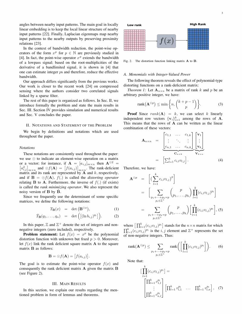
IV. NUMERICAL RESULTSFor the purpose of simulation results, we have implemented

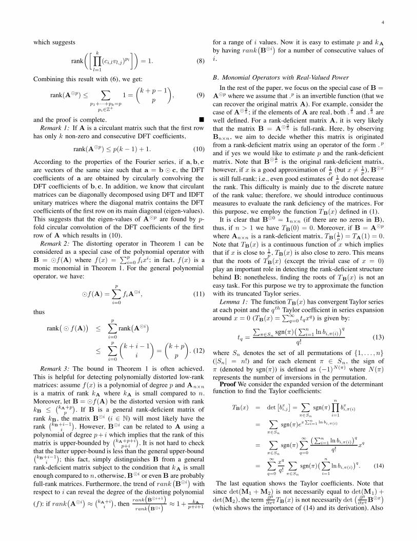
the algorithms for both the integer and the real-valued powersin MATLAB. In the first scenario, we have generated a lowrank matrix by multiplying two 1000&5 and 5&1000 randommatrices with i.i.d. elements uniformly distributed in [0, 1].The resultant matrix which is of rank 5 is used as the originallow rank matrix while its distorted version is constructedas B = A#2. According to Theorem 1, we should haverank

!A#p

"#

!4+pp

"for a positive integer p; in fact, Fig.

3 confirms that the equality happens for this matrix1. On the

1Due to the numerical errors, MATLAB’s rank function is inaccurate forlarge rank-deficient matrices; for determining the rank, we have used the gapbetween the singular values to distinguish between the zero and non-zerovalues.

7

1 2 3 4 5 6 7 8 9 100

100

200

300

400

500

600

700

800

900

1000

p

Ran

k

C(14+p , p)BC(4+p , p)A

Fig. 3. The rank of the 1000 # 1000 matrices A%p,B%p versus integerp where B = A%2. The rank of the matrices A and B are 5 and 15,respectively, which imply upper bounds of the form

!4+pp

"and

!14+pp

"on

the ranks of A%p,B%p.

0 1 2 3 4 5 6 7 8 9 10

10 300

10 200

10 100

100

10100

10200

| det

(.) |

NoiselessSNR=100dBSNR= 75dBSNR= 50dB

x

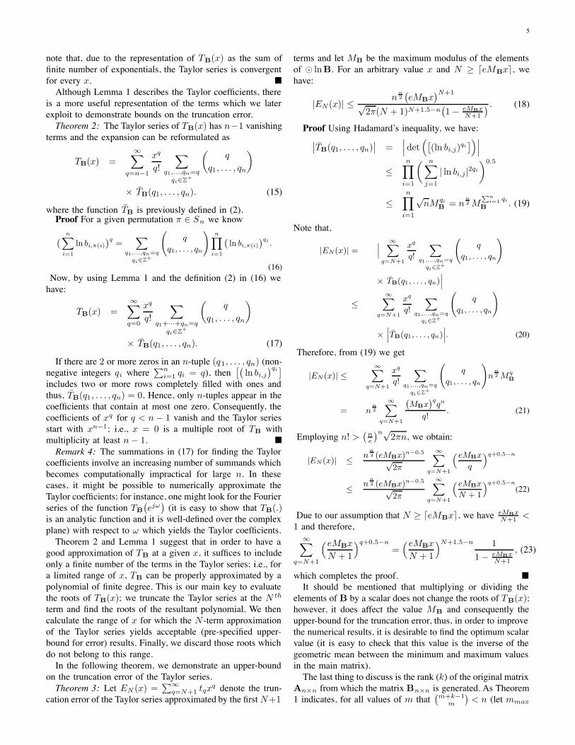
Fig. 4. The determinant of B%x and its noisy versions versus x; the largenegative peaks in the log scale indicate the existence of roots (rank minimizingpower).

other hand, for the matrix B where we have rank(B) = 15,there is a gap between the upper bound

!14+pp

"and the actual

rank. It is easy to check that the rank curve of B#p coincideswith

!4+2p2p

"; this is in fact the key to find the rank of A by

having B (as explained in Remark 3).In the second scenario, we have considered a circulant rank-

deficient matrix. The first row of this 100 & 100 matrix isgenerated in such a way that it has only 5 non-zero and con-secutive DFT coefficients; in fact the non-zero coefficients aregenerated by realizations of i.i.d. zero-mean normal randomvariables with variance 10. The applied distorting operatorhere is .# 5

11 ; i.e., p = 511 and the original rank-deficient matrix

A100!100 is recovered by taking the elements of the distortedmatrix B100!100 to the power 1

p = 2.2. In order to includethe noise effect, in addition to implementing the techniques onthe noiseless matrix, the noisy versions of B are also studied:the elements of B are subject to Additive White GaussianNoise (AWGN) with difference noise variances resulting inSNR values 100dB, 75dB and 50dB. Before we conductthe experiments to find the rank minimizing operator, itis interesting to examine the suitability of the determinantfunction for this purpose. Figure 4 depicts the curve of thefunction TB(x) and the corresponding functions for the noisy

0 1 2 3 4 5 6 7 8 9 10103

104

105

106

107

108

109

1010

x

Con

d. N

umbe

r

NoiselessSNR=100dBSNR= 75dBSNR= 50dB

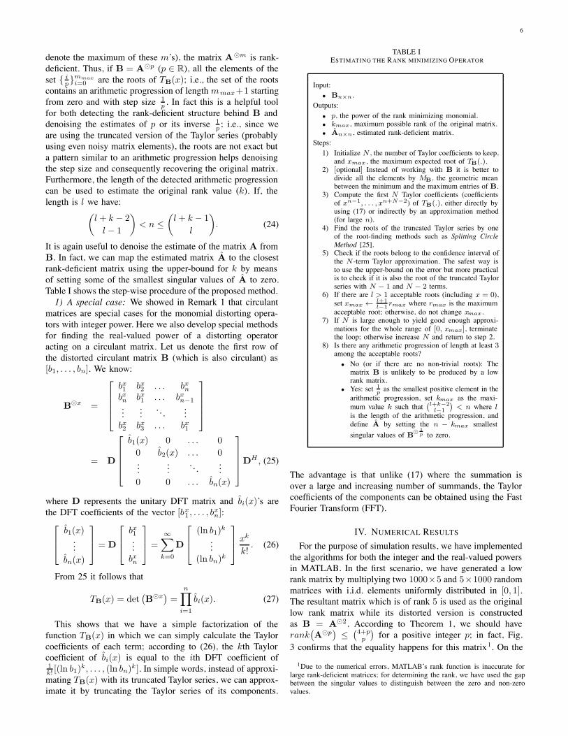
Fig. 5. The condition number of B%x and its noisy versions versus x; thelarge positive peaks might indicate the existence of roots (rank minimizingpower).

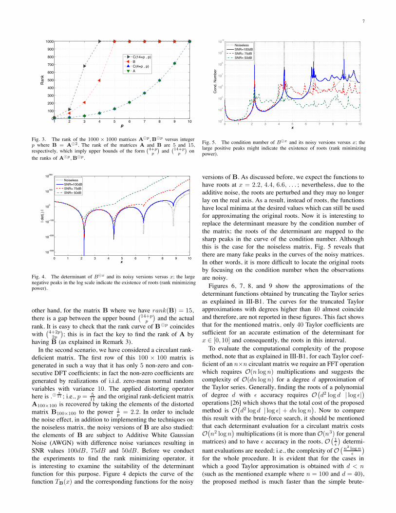
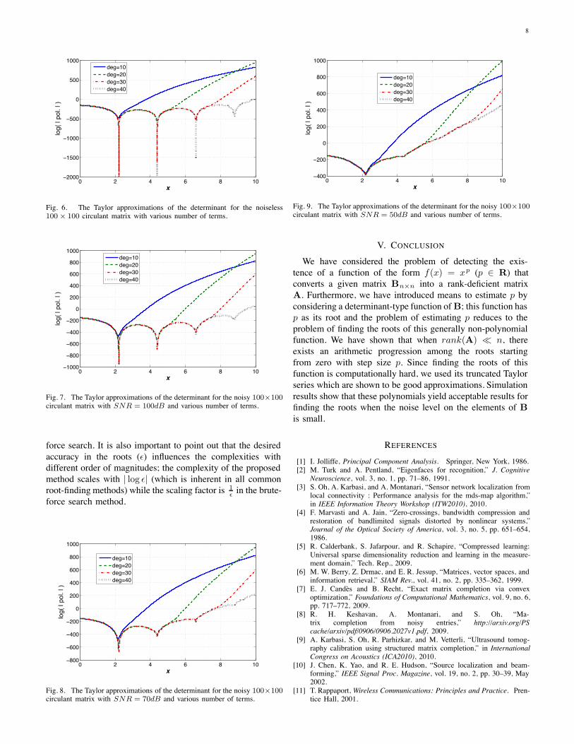
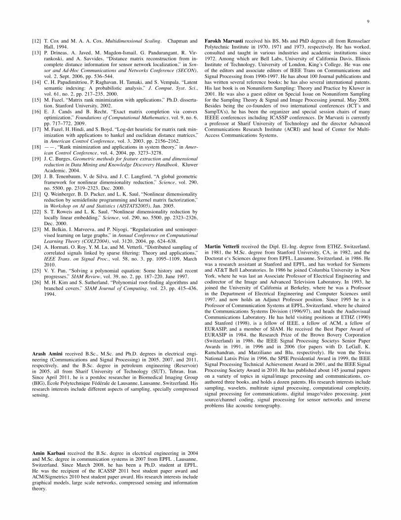
versions of B. As discussed before, we expect the functions tohave roots at x = 2.2, 4.4, 6.6, . . . ; nevertheless, due to theadditive noise, the roots are perturbed and they may no longerlay on the real axis. As a result, instead of roots, the functionshave local minima at the desired values which can still be usedfor approximating the original roots. Now it is interesting toreplace the determinant measure by the condition number ofthe matrix; the roots of the determinant are mapped to thesharp peaks in the curve of the condition number. Althoughthis is the case for the noiseless matrix, Fig. 5 reveals thatthere are many fake peaks in the curves of the noisy matrices.In other words, it is more difficult to locate the original rootsby focusing on the condition number when the observationsare noisy.Figures 6, 7, 8, and 9 show the approximations of the

determinant functions obtained by truncating the Taylor seriesas explained in III-B1. The curves for the truncated Taylorapproximations with degrees higher than 40 almost coincideand therefore, are not reported in these figures. This fact showsthat for the mentioned matrix, only 40 Taylor coefficients aresufficient for an accurate estimation of the determinant forx $ [0, 10] and consequently, the roots in this interval.To evaluate the computational complexity of the propose

method, note that as explained in III-B1, for each Taylor coef-ficient of an n&n circulant matrix we require an FFT operationwhich requires O(n logn) multiplications and suggests thecomplexity of O(dn logn) for a degree d approximation ofthe Taylor series. Generally, finding the roots of a polynomialof degree d with % accuracy requires O

!d2 log d | log %|

"

operations [26] which shows that the total cost of the proposedmethod is O

!d2 log d | log %| + dn logn

". Now to compare

this result with the brute-force search, it should be mentionedthat each determinant evaluation for a circulant matrix costsO!n2 logn

"multiplications (it is more thanO(n3) for general

matrices) and to have % accuracy in the roots, O!1%

"determi-

nant evaluations are needed; i.e., the complexity ofO!n2 logn

%

"

for the whole procedure. It is evident that for the cases inwhich a good Taylor approximation is obtained with d < n(such as the mentioned example where n = 100 and d = 40),the proposed method is much faster than the simple brute-

8

0 2 4 6 8 102000

1500

1000

500

0

500

1000

x

log(

| po

l. | )

deg=10deg=20deg=30deg=40

Fig. 6. The Taylor approximations of the determinant for the noiseless100 # 100 circulant matrix with various number of terms.

0 2 4 6 8 101000

800

600

400

200

0

200

400

600

800

1000

x

log(

| po

l. | )

deg=10deg=20deg=30deg=40

Fig. 7. The Taylor approximations of the determinant for the noisy 100#100circulant matrix with SNR = 100dB and various number of terms.

force search. It is also important to point out that the desiredaccuracy in the roots (%) influences the complexities withdifferent order of magnitudes; the complexity of the proposedmethod scales with | log %| (which is inherent in all commonroot-finding methods) while the scaling factor is 1

% in the brute-force search method.

0 2 4 6 8 10800

600

400

200

0

200

400

600

800

1000

x

log(

| po

l. | )

deg=10deg=20deg=30deg=40

Fig. 8. The Taylor approximations of the determinant for the noisy 100#100circulant matrix with SNR = 70dB and various number of terms.

0 2 4 6 8 10400

200

0

200

400

600

800

1000

x

log(

| po

l. | )

deg=10deg=20deg=30deg=40

Fig. 9. The Taylor approximations of the determinant for the noisy 100#100circulant matrix with SNR = 50dB and various number of terms.

V. CONCLUSION

We have considered the problem of detecting the exis-tence of a function of the form f(x) = xp (p $ R) thatconverts a given matrix Bn!n into a rank-deficient matrixA. Furthermore, we have introduced means to estimate p byconsidering a determinant-type function ofB; this function hasp as its root and the problem of estimating p reduces to theproblem of finding the roots of this generally non-polynomialfunction. We have shown that when rank(A) - n, thereexists an arithmetic progression among the roots startingfrom zero with step size p. Since finding the roots of thisfunction is computationally hard, we used its truncated Taylorseries which are shown to be good approximations. Simulationresults show that these polynomials yield acceptable results forfinding the roots when the noise level on the elements of Bis small.

REFERENCES[1] I. Jolliffe, Principal Component Analysis. Springer, New York, 1986.[2] M. Turk and A. Pentland, “Eigenfaces for recognition,” J. Cognitive

Neuroscience, vol. 3, no. 1, pp. 71–86, 1991.[3] S. Oh, A. Karbasi, and A. Montanari, “Sensor network localization from

local connectivity : Performance analysis for the mds-map algorithm,”in IEEE Information Theory Workshop (ITW2010), 2010.

[4] F. Marvasti and A. Jain, “Zero-crossings, bandwidth compression andrestoration of bandlimited signals distorted by nonlinear systems,”Journal of the Optical Society of America, vol. 3, no. 5, pp. 651–654,1986.

[5] R. Calderbank, S. Jafarpour, and R. Schapire, “Compressed learning:Universal sparse dimensionality reduction and learning in the measure-ment domain,” Tech. Rep., 2009.

[6] M. W. Berry, Z. Drmac, and E. R. Jessup, “Matrices, vector spaces, andinformation retrieval,” SIAM Rev., vol. 41, no. 2, pp. 335–362, 1999.

[7] E. J. Candes and B. Recht, “Exact matrix completion via convexoptimization,” Foundations of Computational Mathematics, vol. 9, no. 6,pp. 717–772, 2009.

[8] R. H. Keshavan, A. Montanari, and S. Oh, “Ma-trix completion from noisy entries,” http://arxiv.org/PScache/arxiv/pdf/0906/0906.2027v1.pdf, 2009.

[9] A. Karbasi, S. Oh, R. Parhizkar, and M. Vetterli, “Ultrasound tomog-raphy calibration using structured matrix completion,” in InternationalCongress on Acoustics (ICA2010), 2010.

[10] J. Chen, K. Yao, and R. E. Hudson, “Source localization and beam-forming,” IEEE Signal Proc. Magazine, vol. 19, no. 2, pp. 30–39, May2002.

[11] T. Rappaport, Wireless Communications: Principles and Practice. Pren-tice Hall, 2001.

9

[12] T. Cox and M. A. A. Cox, Multidimensional Scaling. Chapman andHall, 1994.

[13] P. Drineas, A. Javed, M. Magdon-Ismail, G. Pandurangant, R. Vir-rankoski, and A. Savvides, “Distance matrix reconstruction from in-complete distance information for sensor network localization,” in Sen-sor and Ad-Hoc Communications and Networks Conference (SECON),vol. 2, Sept. 2006, pp. 536–544.

[14] C. H. Papadimitriou, P. Raghavan, H. Tamaki, and S. Vempala, “Latentsemantic indexing: A probabilistic analysis,” J. Comput. Syst. Sci.,vol. 61, no. 2, pp. 217–235, 2000.

[15] M. Fazel, “Matrix rank minimization with applications,” Ph.D. disserta-tion, Stanford University, 2002.

[16] E. J. Cands and B. Recht, “Exact matrix completion via convexoptimization,” Foundations of Computational Mathematics, vol. 9, no. 6,pp. 717–772, 2009.

[17] M. Fazel, H. Hindi, and S. Boyd, “Log-det heuristic for matrix rank min-imization with applications to hankel and euclidean distance matrices,”in American Control Conference, vol. 3, 2003, pp. 2156–2162.

[18] ——, “Rank minimization and applications in system theory,” in Amer-ican Control Conference, vol. 4, 2004, pp. 3273–3278.

[19] J. C. Burges, Geometric methods for feature extraction and dimensionalreduction in Data Mining and Knowledge Discovery Handbook. KluwerAcademic, 2004.

[20] J. B. Tenenbaum, V. de Silva, and J. C. Langford, “A global geometricframework for nonlinear dimensionality reduction,” Science, vol. 290,no. 5500, pp. 2319–2323, Dec. 2000.

[21] Q. Weinberger, B. D. Packer, and L. K. Saul, “Nonlinear dimensionalityreduction by semidefinite programming and kernel matrix factorization,”in Workshop on AI and Statistics (AISTATS2005), Jan. 2005.

[22] S. T. Roweis and L. K. Saul, “Nonlinear dimensionality reduction bylocally linear embedding,” Science, vol. 290, no. 5500, pp. 2323–2326,Dec. 2000.

[23] M. Belkin, I. Matveeva, and P. Niyogi, “Regularization and semisuper-vised learning on large graphs,” in Annual Conference on ComputationalLearning Theory (COLT2004), vol. 3120, 2004, pp. 624–638.

[24] A. Hormati, O. Roy, Y. M. Lu, and M. Vetterli, “Distributed sampling ofcorrelated signals linked by sparse filtering: Theory and applications,”IEEE Trans. on Signal Proc., vol. 58, no. 3, pp. 1095–1109, March2010.

[25] V. Y. Pan, “Solving a polynomial equation: Some history and recentprogresses,” SIAM Review, vol. 39, no. 2, pp. 187–220, June 1997.

[26] M. H. Kim and S. Sutherland, “Polynomial root-finding algorithms andbranched covers,” SIAM Journal of Computing, vol. 23, pp. 415–436,1994.

Arash Amini received B.Sc., M.Sc. and Ph.D. degrees in electrical engi-neering (Communications and Signal Processing) in 2005, 2007, and 2011,respectively, and the B.Sc. degree in petroleum engineering (Reservoir)in 2005, all from Sharif University of Technology (SUT), Tehran, Iran.Since April 2011, he is a postdoc researcher in Biomedical Imaging Group(BIG), Ecole Polytechnique Federale de Lausanne, Lausanne, Switzerland. Hisresearch interests include different aspects of sampling, specially compressedsensing.

Amin Karbasi received the B.Sc. degree in electrical engineering in 2004and M.Sc. degree in communication systems in 2007 from EPFL , Lausanne,Switzerland. Since March 2008, he has been a Ph.D. student at EPFL.He was the recipient of the ICASSP 2011 best student paper award andACM/Sigmetrics 2010 best student paper award. His research interests includegraphical models, large scale networks, compressed sensing and informationtheory.

Farokh Marvasti received his BS, Ms and PhD degrees all from RensselaerPolytechnic Institute in 1970, 1971 and 1973, respectively. He has worked,consulted and taught in various industries and academic institutions since1972. Among which are Bell Labs, University of California Davis, IllinoisInstitute of Technology, University of London, King’s College. He was oneof the editors and associate editors of IEEE Trans on Communications andSignal Processing from 1990-1997. He has about 100 Journal publications andhas written several reference books; he has also several international patents.His last book is on Nonuniform Sampling: Theory and Practice by Kluwer in2001. He was also a guest editor on Special Issue on Nonuniform Samplingfor the Sampling Theory & Signal and Image Processing journal, May 2008.Besides being the co-founders of two international conferences (ICT’s andSampTA’s), he has been the organizer and special session chairs of manyIEEEE conferences including ICASSP conferences. Dr Marvasti is currentlya professor at Sharif University of Technology and the director AdvancedCommunications Research Institute (ACRI) and head of Center for Multi-Access Communications Systems.

Martin Vetterli received the Dipl. El.-Ing. degree from ETHZ, Switzerland,in 1981, the M.Sc. degree from Stanford University, CA, in 1982, and theDoctorat e‘s Sciences degree from EPFL, Lausanne, Switzerland, in 1986. Hewas a research assistant at Stanford and EPFL, and has worked for Siemensand AT&T Bell Laboratories. In 1986 he joined Columbia University in NewYork, where he was last an Associate Professor of Electrical Engineering andcodirector of the Image and Advanced Television Laboratory. In 1993, hejoined the University of California at Berkeley, where he was a Professorin the Department of Electrical Engineering and Computer Sciences until1997, and now holds an Adjunct Professor position. Since 1995 he is aProfessor of Communication Systems at EPFL, Switzerland, where he chairedthe Communications Systems Division (1996/97), and heads the AudiovisualCommunications Laboratory. He has held visiting positions at ETHZ (1990)and Stanford (1998), is a fellow of IEEE, a fellow of ACM, a fellow ofEURASIP, and a member of SIAM. He received the Best Paper Award ofEURASIP in 1984, the Research Prize of the Brown Bovery Corporation(Switzerland) in 1986, the IEEE Signal Processing Societys Senior PaperAwards in 1991, in 1996 and in 2006 (for papers with D. LeGall, K.Ramchandran, and Marziliano and Blu, respectively). He won the SwissNational Latsis Prize in 1996, the SPIE Presidential Award in 1999, the IEEESignal Processing Technical Achievement Award in 2001, and the IEEE SignalProcessing Society Award in 2010. He has published about 145 journal paperson a variety of topics in signal/image processing and communications, co-authored three books, and holds a dozen patents. His research interests includesampling, wavelets, multirate signal processing, computational complexity,signal processing for communications, digital image/video processing, jointsource/channel coding, signal processing for sensor networks and inverseproblems like acoustic tomography.