A Numerical Investigation of the Local Ocean Response to ... · A Numerical Investigation of the Local Ocean Response to Westerly Wind ... ship transects in the ... is determined

1334 VOLUME 29J O U R N A L O F P H Y S I C A L O C E A N O G R A P H Y

q 1999 American Meteorological Society

A Numerical Investigation of the Local Ocean Response to Westerly Wind BurstForcing in the Western Equatorial Pacific

RAYMOND A. RICHARDSON, ISAAC GINIS, AND LEWIS M. ROTHSTEIN

Graduate School of Oceanography, University of Rhode Island, Narragansett, Rhode Island

(Manuscript received 9 March 1998, in final form 18 September 1998)

ABSTRACT

Numerical simulations of the local equatorial ocean response to idealized westerly wind burst (WWB) forcingare described. In particular, the authors examine the development and evolution of the subsurface westward jet(SSWJ) that has been observed to accompany these wind events. This westward current is interpreted as thesignature of equatorial waves that accompany the downwelling and upwelling that occurs along the edges ofthe wind forcing region. Some important features of the SSWJ include maximum intensity toward the easternedge of the forcing region, a time lag between the wind forcing and peak SSWJ development, and an eastwardspreading of the SSWJ with time. The effect of wind burst zonal profile, magnitude, duration, and fetch on theSSWJ are explored. The response of an initially resting ocean to WWB forcing is compared with that for modeloceans that are spun up with annual-mean surface fluxes and monthly varying fluxes. It is demonstrated thatthe gross features of the response for the spun up simulations can be well approximated by adding the backgroundzonal current structure prior to the introduction of the wind burst to the initially resting ocean current responseto the WWB. This result suggests that the zonal current structure that is present prior to the commencement ofWWB forcing plays a key role in determining whether or not a SSWJ will develop.

1. Introduction

Easterly trade winds predominate over most of theequatorial Pacific, and the ocean response to these windstypically consists of a westward South Equatorial Cur-rent (SEC) and an eastward, subsurface Equatorial Un-dercurrent (EUC) in the immediate vicinity of the equa-tor. In the western Pacific Ocean, the prevailing easterlytrade winds are periodically interrupted by episodes ofstrong westerly wind, occurring typically in boreal win-ter and spring. These wind bursts have zonal extentsthat range from 108 to 408 of longitude, have maximumwinds as high as 15 m s21, and last anywhere from acouple of days to two weeks. In recent years, there hasbeen considerable interest in these westerly wind bursts(WWBs) and their impact on both local and far-fieldocean behavior. In the latter case, it has been suggestedthat eastward propagating Kelvin waves generated byWWBs can play a role in the warming of the easternPacific during El Nino events (Keen 1982; Harrison andGiese 1988).

Regarding the local response, it has long been rec-ognized that strong westerly wind forcing on or near

Corresponding author address: Dr. Raymond A. Richardson, Grad-uate School of Oceanography, University of Rhode Island, Narra-gansett, RI 02822.E-mail: [email protected]

the equator leads to the development of an eastwardsurface Yoshida jet (Yoshida 1959). Less well under-stood has been the phenomenon, first observed by His-ard et al. (1970), that this surface response is often ac-companied by a significant subsurface current directedto the west. Other observations of this subsurface west-ward jet (SSWJ), centered at depths in the 150-m range,were also reported by McPhaden et al. (1992), whopresented current meter data from a Tropical Atmo-sphere Ocean Array buoy located at 08, 1658E and fromship transects in the region. Since that time, additionalobservations of the SSWJ have been made by manyothers (Delcroix et al. 1993a; Kuroda and McPhaden1993). Most recently, observations during the TOGACOARE Intensive Observation Period experiment (1November 1992–28 February 1993), an interval markedby several strong WWBs, also revealed significant west-ward flow between an eastward surface jet and the EUC(Delcroix et al. 1993b; Eldin et al. 1994; Delcroix andEldin 1995; Smyth et al. 1996; Wijesekera et al. 1996).

Efforts to numerically simulate the ocean response toWWBs have focused primarily on the far-field behavior(Giese and Harrison 1990, 1991; Kindle and Phoebus1995). Studies of the local response have been morelimited. McPhaden et al. (1988) presented a one-di-mensional, 1½-layer model that reproduced the devel-opment of strong vertical velocity shear in response toWWB forcing, but the simplicity of that analysis didnot allow consideration of the full three-dimensional

JUNE 1999 1335R I C H A R D S O N E T A L .

aspects of the ocean response. Eriksen (1993) presenteda numerical study of the ocean response to rapidly trans-lating wind bursts and found that, for forcing of thattype, the gravity wave response may dominate the cur-rent and internal displacement fields in the upper ocean.This is because other parts of the equatorial wave spec-trum, such as Kelvin waves, cannot be excited by forc-ing fields whose rate of translation exceeds the wavepropagation speeds. The Erikson analysis was based ona study by Nakazawa (1988), where it was suggestedthat WWBs were associated with disturbances in thetropospheric circulation know as Madden–Julian intra-seasonal oscillations and translated eastward at speedsof approximately 10 m s21. However, historical analysesof long-term data-assimilated atmospheric model prod-ucts (Hartten 1996; Phoebus and Kindle 1994; Harrisonand Vecchi 1997) have indicated that WWBs are oftenassociated with developing tropical cyclones in one orboth hemispheres and can be quite stationary in time,or even move slowly to the west as the storms associatedwith them move in that direction.

More recently Zhang and Rothstein (1998) have in-vestigated the local ocean response to WWB forcingusing a primitive equation model. In that work, it wasshown that a short zonal wind fetch is conducive to thedevelopment of a SSWJ under the center of the forcingregion on timescales of 10 days. However, that studywas restricted to an investigation of the ocean responseduring the initial period in which the wind forcing wasapplied. The purpose of the present study is to explorethe physics of the local dynamical response to near-stationary equatorial WWBs and, in particular, to elu-cidate the principal features of and the mechanism be-hind the SSWJ. This work is in many ways an extensionof the work of Zhang and Rothstein (1998) to broaderspatial and temporal regimes.

A series of experiments will be presented that inves-tigate the local ocean dynamical response to WWB forc-ing and the manner in which that response changes whenvarious aspects of the forcing field are altered. The restof this paper is organized as follows: section 2 describespertinant aspects of the model formulation, section 3details the results of a series of experiments in whicha range of parameters related to the wind field are variedin the context of an initially resting ocean, section 4explores the influence of background current on the oceanresponse, and conclusions are presented in section 5.

2. Model description

a. Model physics

For the experiments described in this study, we em-ploy a nested-grid ocean general circulation model thatprovides high horizontal resolution in the forcing regionwhile still allowing for the computation of a large-scalesurrounding domain. This enables waves to propagatefrom the forcing region without the influence of domain

boundaries and allows for high-resolution regional ex-periments to be conducted in the context of a basin-scale circulating background current field. This hydro-static, primitive equation model is described in detailin Ginis et al. (1998). The model employs the reduced-gravity approximation, that is, only the upper ocean isactively simulated, with a motionless abyssal layer be-low. The vertical axis is partitioned according to a sigmacoordinate in the manner of Gent and Cane (1989). Ver-tical mixing in the model occurs through a combinationof several processes (Chen et al. 1994): a surface mixedlayer undergoes mass exchange with the layer belowaccording to a bulk turbulent kinetic energy balance(Kraus and Turner 1967), vertical mixing in the interioris determined by a Richardson number stability crite-rion, and finally, if necessary, the model is convectivelyadjusted to maintain hydrostatic stability. The momen-tum, heat, and continuity equations are solved and theprognostic variables of temperature, salinity, and ve-locity are calculated. The horizontal diffusion terms arecalculated using the scales of motion resolved by themodel and the local deformation field (Smagorinsky1963). The density is calculated using the modifiedUNESCO equation of state (UNESCO 1981).

b. Grid nesting

The grid nesting procedure, motivated by the desireto more effectively resolve the local response to WWBs,involves a two-way interaction between adjacent mesheswith the conservation properties of mass, momentum,and heat maintained across the grid interfaces (Ginis etal. 1998). In the experiments described below, one totwo inner meshes are telescopically embedded in acoarser-resolution large-scale domain with inner gridresolutions two to three times finer then the surroundinggrid, depending upon the particular experimental setup.In all of the experiments, the WWB forcing is appliedwithin the finest resolution domain.

c. Model geometry

The experiments to be described fall into two generalcategories: resting ocean and circulating ocean. In theresting ocean experiments, a rectangular domain is usedwith boundaries at 108S and 108N in the meridionaldirection and at 1308E and 1308W in the zonal direction.Two grids are used for the resting ocean case, with theresolutions and grid locations indicated in Table 1.

The circulating ocean experiments are performed ina full tropical Pacific basin configuration where thecoastline has been smoothed and islands eliminated. Themodel domain for these experiments is from 308S to308N, 1248E to 708W. During the model spinup, a singlegrid was used with 18 resolution in the zonal directionand variable resolution in the meridional direction thatranged from ⅓8 along the equator to as coarse as 28 atthe northern and southern boundaries. For the wind burst


TABLE 1. Grid locations and resolutions for wind burst experiments.

Resting ocean experiments

Grid 1 Grid 2

Circulating ocean experiments

Grid 1 Grid 2 Grid 3

East–west extentNorth–south extentResolution

1308E–1308W‘ 108S–108N

2/38

1508E–180858S–58N

1/68

1248E–708W308S–308N

1/28

1528E–1808108S–108N

1/48

1588E–1758E58S–58N

1/88

TABLE 2. Parameters for numerical experiments.

Expt

Maxwindstress

(N m22)

Dura-tion

(days)Fetch(deg) Edge width

Initialocean state Lat

123456789

10111213

0.20.20.050.10.20.20.20.20.20.20.20.20.2

1010101010

515101010101010

15402020202020201015151515

Gaussian0888888888880808

GaussianGaussianGaussianGaussian

RestRestRestRestRestRestRestRestRestRestRestAnnual spinupSeasonal spinup

08080808080808080828S48S0808

experiments, the spinup model fields were interpolatedonto a three-grid structure. The grid locations and res-olutions for these experiments are also displayed in Ta-ble 1.

The upper ocean is divided into 13 levels for all ofthe experiments presented here. This structure consistsof a dynamically evolving surface mixed layer and athermocline region. The initial mixed layer depth is setto 40 m for the resting ocean experiments and deter-mined from climatology according to a density criterionfor the circulating ocean experiments. The thermoclineregion is divided into the remaining 12 layers accordingto a prespecified ratio. The vertical resolution was ;20m in the range 40–200 m (becoming as fine as 17 munder the deepest portions of the mixed layer during thewind burst experiments) and gradually coarser below.

d. Model initialization and atmospheric forcing

We will explore two scenarios for the circulatingocean experiments that vary according to the type ofsurface forcing applied during the model spinup. In thefirst case, annual-mean surface flux climatology is used(annual spinup), and in the second, monthly surface fluxclimatology is used (seasonal spinup). The model isinitialized with annual mean Levitus (1982) temperatureand salinity for the annual mean experiments and withJanuary climatology for the seasonal case. The hori-zontal boundary conditions in the spinup runs are non-slip and nonflux at all boundaries. However, near thenorthern (southern) boundary of the domain, poleward

of 258N (S), temperature and salinity are gradually re-laxed toward climatology. The model starts from restand is forced by either annual mean or seasonal (month-ly) climatological surface wind stress and heat fluxes.The wind stress is derived from the Florida State Uni-versity (FSU) pseudostress climatology (Goldenbergand O’Brien 1981). The heat flux Q(SSTc) is calculatedusing the simplified bulk formula of Seager et al. (1988),with annual-mean cloud cover from the InternationalSatellite Cloud Climatology Project (Rossow and Schif-fer 1991). We use the total cloud fraction to determinethe heat flux, making no distinction between high, mid-dle, and low clouds. This introduces some inaccuraciesto the heat flux calculation and a small correction isapplied to avoid excessive surface heating in some lo-cations, most notably near the northern Central Amer-ican coast. The Seager et al. algorithm also requireswind speed for the heat flux calculation. This speed wasderived from the FSU wind stress assuming a surfacedrag coefficient of 1.5 3 1023. In the annual spinupexperiment, the surface values of temperature and sa-linity were relaxed back to climatology on a timescaleof 20 days for a mixed layer 30 m deep. This is nec-essary to avoid excessive model drift from climatologywhen forced with constant annual mean fluxes. No suchrelaxation term is required in the seasonal spinup. Themodel is integrated for three years for the annual spinupand for six years for the seasonal spinup. These inte-gration lengths were sufficient to establish quasi equi-librium in the two scenarios, though any slow evolutionof the background state should not strongly influenceour conclusions about the local ocean response on themuch shorter timescales of the wind burst experimentsdescribed in the following sections.

3. Experimental results

The following sections describe the results of a seriesof numerical experiments aimed at illuminating the ba-sic properties of the SSWJ and the factors that affectits behavior and evolution. The various experimentalsettings are summarized in Table 2. The experimentscan be broadly separated into those in which the modelocean was initially at rest and those in which an initialbackground circulation was present. Within the initiallyresting ocean category, the dependence of the oceanresponse on various parameters such as wind-stress zon-al profile, wind duration and magnitude, and wind burstlocation are explored. In the circulating ocean experi-


ments, the response of model oceans with two differentbackground current configurations, the annual and sea-sonal spinups, is compared.

a. Response of an initially resting ocean

1) AN ILLUSTRATIVE CASE

To examine the principal features of the local zonalcurrent response to WWB forcing, a stationary, ideal-ized burst was applied along the equator with zonal windstress described by the following expression:lt 0

2 2 2 2l l 2(l2l ) /L 2(f2f ) /L0 x 0 yt 5 t e e , (1)0 max

where tmax 5 0.2 N m22, Lx 5 7.58, and Ly 5 38. Thesespatial dimensions were chosen to be within the rangeof parameters observed historically (Harrison and Giese1991). The burst was centered at f 0 5 08, l0 5 1658Eand was stationary in time. This wind stress was appliedimpulsively for 10 days and then turned off. The tem-perature and salinity stratification were taken from Lev-itus climatology for the location 08, 1658E and the mixedlayer depth was chosen to be 40 m. Changes in surfaceheat and freshwater flux associated with the wind burstare neglected in this and all the following experiments.Since our primary focus is on the dynamical response,we believe this is a reasonable simplification. This con-figuration will be referred to as experiment 1.

Figure 1 shows zonal slices along the equator of thezonal velocity field every 5 days for the first 30 daysafter the initial imposition of the wind burst forcing.Two features are immediately evident: a wind-driveneastward near-surface Yoshida jet and a westward SSWJbelow. The surface jet accelerates for the duration ofthe wind forcing and decelerates thereafter. The SSWJ,on the other hand, does not reach its maximum untilday 20, ten days after the surface forcing has ceased. Itundergoes a gradual eastward and downward spreadingand, with the exception of the earliest times (day 5),shows a consistent eastward bias relative to the centerof the wind burst forcing (1658E). At later times, (days25 and 30), the velocity structure becomes more com-plex and eastward flow below the SSWJ begins to de-velop, with some westward flow to the west of the windburst center at SSWJ depths also becoming evident.

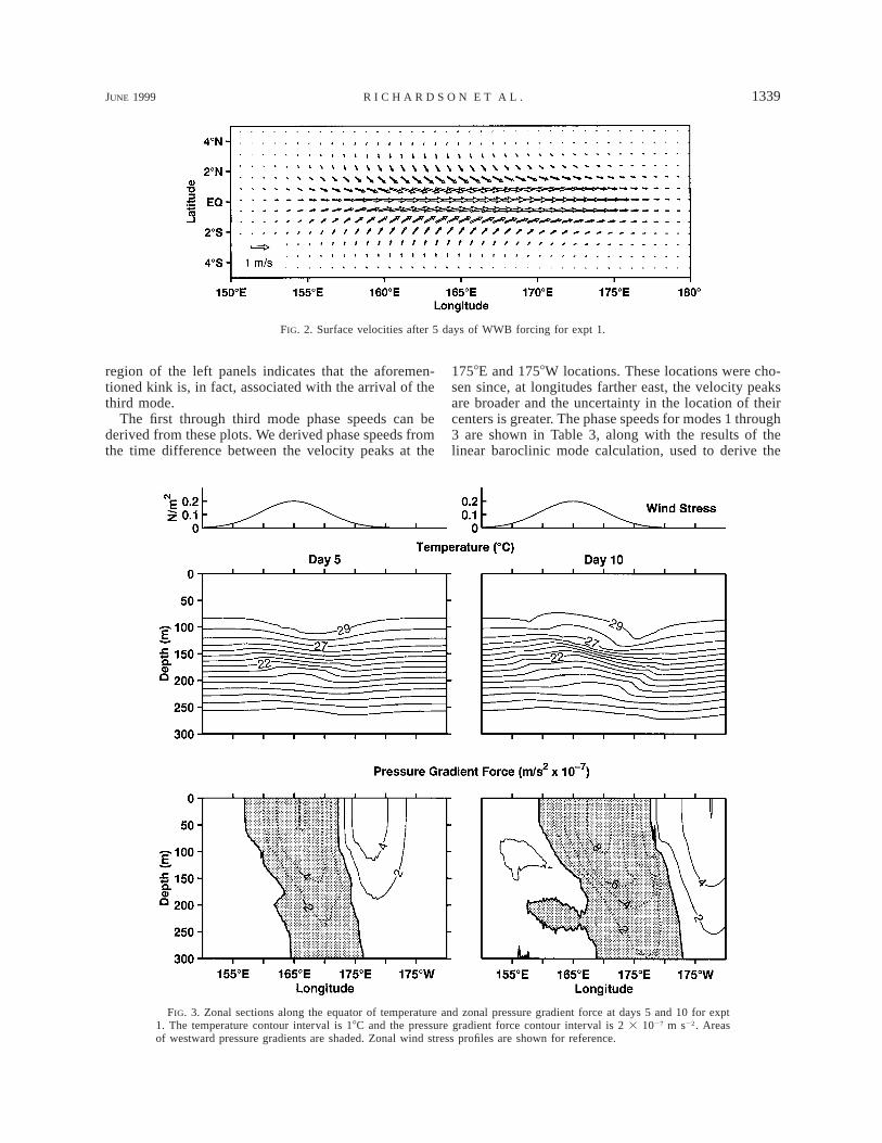
Before examining any of the effects of variations inwind forcing, some interpretation of the results of ex-periment 1 is required. Figure 2 shows the surface ve-locity field after 5 days of wind burst forcing. The zonalcomponent can be seen to be convergent on the easternside and divergent on the western side. The meridionalvelocity field is convergent all along the length of theforcing area, the result of the Coriolis force associatedwith the eastward wind stress. The total surface hori-zontal velocity field that results from these two com-ponents is strongly convergent on the eastern side ofthe forcing region and relatively weakly divergent onthe western side. Continuity requires eastern side down-

welling and western side upwelling, with the down-welling contribution dominating. Associated with thisupwelling and downwelling will be deviations in theupper thermocline structure that will be seen to be di-rectly associated with the subsurface current response,that is, the SSWJ.

To illustrate this point further, Fig. 3 shows zonalsections of temperature (variations of which are the prin-cipal source of density anomalies in this study) andpressure gradient force for experiment 1. The easternside downward deflection of the thermocline is readilyapparent in the upper panels. This deviation has a neg-ative pressure gradient force associated with it (lowerpanels) that is near the center of the forcing region atday 5 but is strongly biased toward the east by day 10.The westward subsurface current development shownin Fig. 1 can be seen to closely correspond to the lo-cation of the negative pressure gradient force.

Figure 4 shows the vertical structure of the first fourorthonormal baroclinic modes for the density profileused in experiment 1. In the calculation of these modes,the reduced gravity system was approximated by settingthe bottom layer thickness to be very large. The mostimportant feature to note is that modes 2–4 have sig-nificant westward amplitudes at depths of 120–200 m.Higher modes as well will have a westward peak justbelow the mixed layer. This indicates that baroclinicKelvin waves of mode number greater than one that areassociated with downward thermocline displacementson the eastern side of the forcing region will have awestward signature in the region just beneath the mixedlayer. The actual amplitudes that the different verticalmodes take in experiment 1 will also be affected by therelative strength with which they are forced. Since themeridional scale of the windburst in this experiment issomewhat larger than the first baroclinic radius of de-formation, we can expect the projection coefficientsonto the various modes to decrease with increasingmode number. We suggest that the SSWJ is primarilythe signature of the total modal response associated withthe thermocline deviations that arise along the edges ofthe wind forcing region.

The development of baroclinic Kelvin modes on theeastern side of the forcing region can be observed inthe time series of Fig. 1. The first eastward propagatingfeature that emerges is the surface-concentrated east-ward signal associated with the first Kelvin mode, whichcan be seen leaving the region of the plot on day 25.Trailing that signal, the slower moving second modebecomes apparent, with an eastward surface flow and awestward flow below. As the second mode moves awayfrom the forcing region, the third baroclinic mode, withan east–west–east zonal velocity structure as one movesdown the water column, is visible in the day 25 andday 30 plots in the vicinity of 1758E.

The development and eastward propagation of thesebaroclinic modes is further illustrated in Fig. 5. Thisfigure shows time series of the zonal velocity on the


FIG. 1. Zonal sections along the equator of the zonal velocity (cm s21) for expt 1. Contour intervals are every 10 cms21. Regions of westward velocity are shaded and regions with westward velocities in excess of 20 cm s21 are darklyshaded. Zonal wind stress profiles are included for reference.

equator at depths of 150 and 350 m at several differentlongitudes to the east of the center of the WWB. Theleft panels display the propagation of the (positive) firstKelvin mode pulse rapidly to the east followed by along-lived change to westward flow as the second andhigher baroclinic Kelvin modes propagate by the variouslongitudes. At this depth, the second mode responsecannot be easily distinguished from the third mode,though a slight, eastward propagating kink in the plotsmay be indicative of the arrival of the third mode signal.

We argue that this blending of the westward signals ofdifferent modes in the 150-m depth range is a primarycomponent of the SSWJ feature. At the greater depthof 350 m (right panels) there is a difference in signbetween the second and third modes. The arrival of thenegative second mode signal, and the eventual sign re-versal that indicates the passage of the third mode, isclearly visible at this depth. The close temporal corre-spondence between the change to positive velocities inthe right panels and the kink in the negative velocity


FIG. 2. Surface velocities after 5 days of WWB forcing for expt 1.

FIG. 3. Zonal sections along the equator of temperature and zonal pressure gradient force at days 5 and 10 for expt1. The temperature contour interval is 18C and the pressure gradient force contour interval is 2 3 1027 m s22. Areasof westward pressure gradients are shaded. Zonal wind stress profiles are shown for reference.

region of the left panels indicates that the aforemen-tioned kink is, in fact, associated with the arrival of thethird mode.

The first through third mode phase speeds can bederived from these plots. We derived phase speeds fromthe time difference between the velocity peaks at the

1758E and 1758W locations. These locations were cho-sen since, at longitudes farther east, the velocity peaksare broader and the uncertainty in the location of theircenters is greater. The phase speeds for modes 1 through3 are shown in Table 3, along with the results of thelinear baroclinic mode calculation, used to derive the


FIG. 4. Normalized vertical structure functions for the first fourbaroclinic modes corresponding to the density structure of expt 1.Symbols indicate the location of model levels.

TABLE 3. Kelvin wave phase speeds for expt 1.

Mode

Deformationradius(km)

Phase speed–analytical(m s21)

Phase speed–model(m s21)

123

247158125

2.801.150.72

2.991.140.78

FIG. 5. Time series of the zonal velocity at 150- and 350-m depths at various longitudes forexpt 1.

vertical structure functions displayed in Fig. 4. Themodel phase speeds agree with the analytical calculationwithin 10%. This lends support to the baroclinic modeinterpretation outlined above.

Associated with the generation and eastward propa-gation of the various baroclinic Kelvin waves at theirrespective velocities is an evolution of the region ofsubsurface westward flow. The SSWJ, which we willarbitrarily define to be the region encompassed by the220 cm s21 zonal velocity contour, is characterized byseveral features enumerated above: an eastward bias rel-ative to the wind burst center, a delayed maximum rel-ative to the surface jet, and a gradual eastward anddownward spreading. Each of these features can be in-terpreted within the context of the baroclinic mode de-scription. The eastward bias is a reflection of the pro-posed forcing mechanism, pressure gradients associatedwith downwelling of the thermocline along the surface-


convergent eastern side of the forcing region. The timelag in maximum current can be attributed to severalfactors. First, since the waves are being forced by thethermocline deviation (and the associated pressure gra-dient) rather than directly by the surface stress itself,they can continue to accelerate as long as the pressuregradient associated with this deviation has not beeneliminated by the ocean adjustment process. Second, thefirst baroclinic Kelvin mode has a significant eastwardamplitude at SSWJ depths (see Fig. 4) and therefore theSSWJ does not reach its maximum until the first modepulse has moved away. This feature will be explored inmore detail in some of the experiments to be describedbelow. The last feature, the eastward spreading of theSSWJ, supports the hypothesis that the SSWJ comprisesthe superposition of several baroclinic modes that prop-agate with different eastward phase velocities, resultingin a broadening of the feature to the east over time.

This illustrative case has served to highlight some ofthe principal features of the local dynamical responseto a WWB. Within this general qualitative framework,significant variations can take place that depend on thedetails of the wind stress spatial and temporal structure.Some of these variations will be examined in the fol-lowing sections.

2) STEP-FUNCTION ZONAL WIND PROFILE

The selection of a smooth, Gaussian wind-stress pro-file in the above experiment was intended to reflect thesort of spatial wind variations that one might expect, atleast in an aggregate sense, in real WWBs (Harrisonand Vecchi 1997). It is instructive, however, to examinean even more idealized case, where the wind stress pro-file varies as a step function. The zonal variation in windstress magnitude for this experiment, referred to as ex-periment 2, is given by the following:

t , l # l # lmax 1 2lt 5 (2)0 50, l , l , l , l.1 2

Here tmax is again 0.2 N m22 and l1 and l2 are 1458Eand 1758W, respectively. The rather long 408 zonal fetch,in conjunction with the step-function wind shape, willserve to isolate the contributions to the overall responsefrom the different waves generated along the easternand western edges. This will enable us to determinesome of the individual wave processes that may havecombined to form the broad response of experiment 1.

The zonal velocity profiles along the equator are plot-ted in the same fashion as for experiment 1 in Fig. 6.One immediate difference from the smoother wind pro-file case of experiment 1 is that the western edge zonalvelocity divergence is strong enough that the compen-sating effect of meridional convergence is relatively un-important, and the resulting thermocline upwelling onthe western side is comparable in magnitude to the east-ern side downwelling. The consequence of this is that

the western edge of the forcing region in experiment 2is the site of significant wave activity of its own, afeature that was less significant in experiment 1.

From the standpoint of SSWJ generation, Fig. 6 canbe interpreted as follows. The upwelling and down-welling thermocline perturbations on the western andeastern edges, respectively, are accompanied by a spec-trum of waves in both locales. An important feature tonote, however, is that these spectra have opposite sign:that is, while the eastern edge first baroclinic modeKelvin wave has an eastward zonal velocity signature(the ‘‘downwelling’’ Kelvin wave), the western edgefirst mode Kelvin wave (the ‘‘upwelling’’ wave) haswestward velocities associated with it.

We have heretofore focused primarily on eastwardmoving Kelvin waves, but westward propagating Ross-by waves will also be seen to play a role in experiment2. Contrary to the Kelvin wave case, the first baroclinicRossby mode on the upwelling western edge has aneastward velocity signature, while the eastern edge firstbaroclinic Rossby mode has westward velocities alongthe equator.

The day 5 plot in Fig. 6 shows the beginnings of thedevelopment of two westward subsurface velocity max-ima on the edges of the forcing region, each of whichis paired with a neighboring eastward maxima. The ther-mocline depression on the eastern edge produces aneastward acceleration on its eastern half and a westwardacceleration on its western half. The domed isopycnalson the upwelling western edge of the forcing region dojust the opposite. The first upwelling Kelvin mode, thewestward surface velocity of which is masked by theYoshida jet, is seen to emanate from the western edgeand spread to the east with time. The initial signs of awestward propagating first Rossby mode with its east-ward velocity signature can also be seen spreading fromthe western edge. At the eastern edge of the forcingregion, the downwelling conditions are associated witha combination of higher order Kelvin modes as dis-cussed in the context of experiment 1 and the eastern-side first Rossby mode. The eastern edge first Rossbymode, like the first Kelvin mode from the western edge,has its westward surface character masked by the Yosh-ida jet.

By day 10, the eastward propagation of the firstKelvin mode from the western edge and, to a lesserextent, the westward propagation of the first Rossbymode from the eastern edge have narrowed the gap be-tween the two subsurface westward velocity maxima.The first Kelvin wave phase speed is ;2.28 day21 (seeTable 3), which would put the leading edge of the west-ern side first Kelvin pulse near 1678E by day 10. Theday 10 plot has an extra contour line at 23 cm s21 toillustrate this point. One can see that the leading edgeof subsurface westward maximum emanating from thewestern edge of the forcing region, as judged by theposition of this 23 cm s21 contour line, is in very closeagreement with the 1678E prediction.


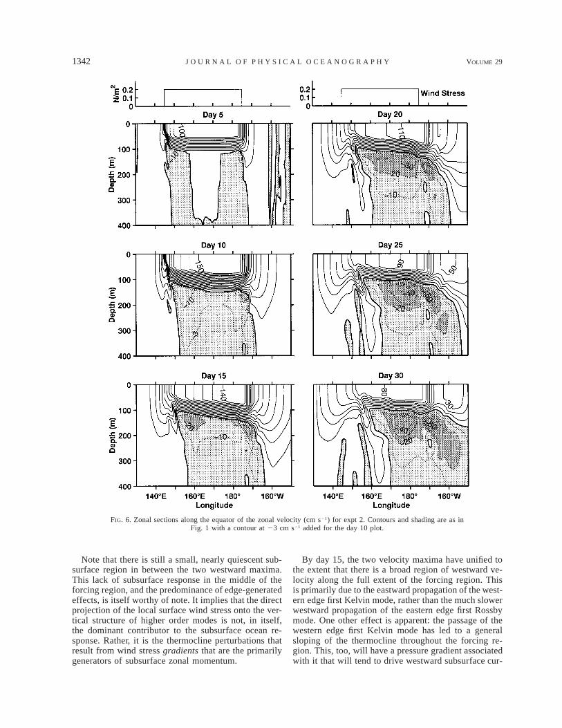
FIG. 6. Zonal sections along the equator of the zonal velocity (cm s21) for expt 2. Contours and shading are as inFig. 1 with a contour at 23 cm s21 added for the day 10 plot.

Note that there is still a small, nearly quiescent sub-surface region in between the two westward maxima.This lack of subsurface response in the middle of theforcing region, and the predominance of edge-generatedeffects, is itself worthy of note. It implies that the directprojection of the local surface wind stress onto the ver-tical structure of higher order modes is not, in itself,the dominant contributor to the subsurface ocean re-sponse. Rather, it is the thermocline perturbations thatresult from wind stress gradients that are the primarilygenerators of subsurface zonal momentum.

By day 15, the two velocity maxima have unified tothe extent that there is a broad region of westward ve-locity along the full extent of the forcing region. Thisis primarily due to the eastward propagation of the west-ern edge first Kelvin mode, rather than the much slowerwestward propagation of the eastern edge first Rossbymode. One other effect is apparent: the passage of thewestern edge first Kelvin mode has led to a generalsloping of the thermocline throughout the forcing re-gion. This, too, will have a pressure gradient associatedwith it that will tend to drive westward subsurface cur-


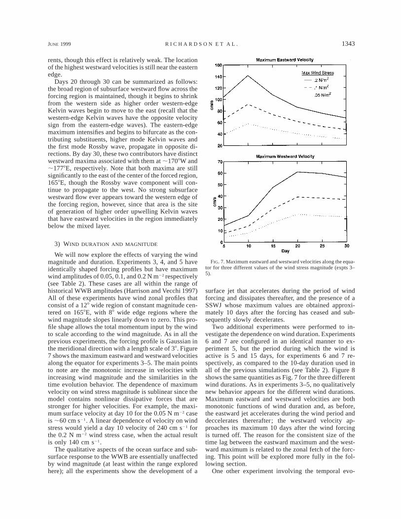
FIG. 7. Maximum eastward and westward velocities along the equa-tor for three different values of the wind stress magnitude (expts 3–5).

rents, though this effect is relatively weak. The locationof the highest westward velocities is still near the easternedge.

Days 20 through 30 can be summarized as follows:the broad region of subsurface westward flow across theforcing region is maintained, though it begins to shrinkfrom the western side as higher order western-edgeKelvin waves begin to move to the east (recall that thewestern-edge Kelvin waves have the opposite velocitysign from the eastern-edge waves). The eastern-edgemaximum intensifies and begins to bifurcate as the con-tributing substituents, higher mode Kelvin waves andthe first mode Rossby wave, propagate in opposite di-rections. By day 30, these two contributors have distinctwestward maxima associated with them at ;1708W and;1778E, respectively. Note that both maxima are stillsignificantly to the east of the center of the forced region,1658E, though the Rossby wave component will con-tinue to propagate to the west. No strong subsurfacewestward flow ever appears toward the western edge ofthe forcing region, however, since that area is the siteof generation of higher order upwelling Kelvin wavesthat have eastward velocities in the region immediatelybelow the mixed layer.

3) WIND DURATION AND MAGNITUDE

We will now explore the effects of varying the windmagnitude and duration. Experiments 3, 4, and 5 haveidentically shaped forcing profiles but have maximumwind amplitudes of 0.05, 0.1, and 0.2 N m22 respectively(see Table 2). These cases are all within the range ofhistorical WWB amplitudes (Harrison and Vecchi 1997)All of these experiments have wind zonal profiles thatconsist of a 128 wide region of constant magnitude cen-tered on 1658E, with 88 wide edge regions where thewind magnitude slopes linearly down to zero. This pro-file shape allows the total momentum input by the windto scale according to the wind magnitude. As in all theprevious experiments, the forcing profile is Gaussian inthe meridional direction with a length scale of 38. Figure7 shows the maximum eastward and westward velocitiesalong the equator for experiments 3–5. The main pointsto note are the monotonic increase in velocities withincreasing wind magnitude and the similarities in thetime evolution behavior. The dependence of maximumvelocity on wind stress magnitude is sublinear since themodel contains nonlinear dissipative forces that arestronger for higher velocities. For example, the maxi-mum surface velocity at day 10 for the 0.05 N m22 caseis ;60 cm s21. A linear dependence of velocity on windstress would yield a day 10 velocity of 240 cm s21 forthe 0.2 N m22 wind stress case, when the actual resultis only 140 cm s21.

The qualitative aspects of the ocean surface and sub-surface response to the WWB are essentially unaffectedby wind magnitude (at least within the range exploredhere); all the experiments show the development of a

surface jet that accelerates during the period of windforcing and dissipates thereafter, and the presence of aSSWJ whose maximum values are obtained approxi-mately 10 days after the forcing has ceased and sub-sequently slowly decelerates.

Two additional experiments were performed to in-vestigate the dependence on wind duration. Experiments6 and 7 are configured in an identical manner to ex-periment 5, but the period during which the wind isactive is 5 and 15 days, for experiments 6 and 7 re-spectively, as compared to the 10-day duration used inall of the previous simulations (see Table 2). Figure 8shows the same quantities as Fig. 7 for the three differentwind durations. As in experiments 3–5, no qualitativelynew behavior appears for the different wind durations.Maximum eastward and westward velocities are bothmonotonic functions of wind duration and, as before,the eastward jet accelerates during the wind period anddeccelerates thererafter; the westward velocity ap-proaches its maximum 10 days after the wind forcingis turned off. The reason for the consistent size of thetime lag between the eastward maximum and the west-ward maximum is related to the zonal fetch of the forc-ing. This point will be explored more fully in the fol-lowing section.

One other experiment involving the temporal evo-


FIG. 8. Maximum eastward and westward velocities along the equa-tor for three different values of WWB forcing duration (expts 5–7).

FIG. 9. Maximum eastward and westward velocities along theequator for three different values of wind fetch (expts 2, 8, and 9).

lution of the wind was performed and should be men-tioned here. It could be argued that the impulsive natureof the wind forcing applied in the previous experimentscould be playing an important role in determining theocean response. To investigate this, an additional ex-periment was performed in which the wind magnitudeevolved as a Gaussian in time with an e-folding time-scale of 10 days (full width). The results (not shown)were almost identical to the impulsively forced case,with the velocity magnitudes somewhat smaller than the10-day impulsive case, reflecting the slightly reducednet momentum flux for the Gaussian temporal evolutionexperiment. The central point that emerges from theseexperiments is that the qualitative nature of the zonalvelocity response along the equator is quite robust andnot sensitive to such parameters as wind magnitude,wind duration, or temporal profile.

4) ZONAL WIND FETCH

Given a constant maximum wind stress magnitudeand fixed spatial gradients along the edges of the forcingregion, the wind stress profile can still be altered byvarying the total zonal fetch. The effect of this sort ofchange was investigated by examining three experi-

mental scenarios, one of which has already been dis-cussed above. In this series of experiments, the steplikewind profile of experiment 2 was used since changingthe width of a Gaussian profile would also involvechanging the wind stress gradients. Such a change could,in itself, affect the ocean response and, hence, wasavoided. The results of experiment 2 were comparedwith two other experiments, which we will refer to asexperiments 8 and 9, in which the total zonal wind fetchwas 208 and 108, respectively. Recall that the zonal fetchfor experiment 2 was 408 (see Table 2). Figure 9 showsthe maximum eastward and westward (SSWJ) velocitieswithin a zonal slice along the equator for the three sizesof wind fetch. Looking first at the upper panel, the max-imum eastward velocity is seen to increase steadily withwind fetch. This reflects the greater total momentuminput by the wind stress for the larger fetch cases. Thetemporal evolution is quite similar for the different cas-es, however, with a steady increase during the forcingperiod and gradual decay thereafter.

The maximum westward velocities in the lower paneldisplay a more complex relationship. Here it is seen thata shorter fetch leads to a more rapid increase in theSSWJ maximum, though the absolute maximum for theduration of the run still increases with increased fetch.


Keeping in mind that the location of this maximumwestward current is near the eastern edge of the forcingregion, this behavior reflects some of the wave dynamicsdiscussed earlier. Two factors in particular play the dom-inant role here: first, the SSWJ along the eastern edgeis enhanced as the western-edge first-mode Kelvin wavepasses by and, second, enhancement occurs when all ofthe eastward first-mode pulse has propagated to the eastof the SSWJ region. Considering the first of these fac-tors, the western-edge first-mode signal starts to developalmost as soon as the wind is turned on. For the shorterfetch cases, this pulse reaches the eastern side of theforcing region more quickly, resulting in greater SSWJmaxima at early times. The first-mode Kelvin wave ve-locity (see Table 3) is ;2.8 m s21 (or ;2.28 day21)along the equator. It takes about 4.5 days, then, for afirst-mode Kelvin pulse to travel 108 of longitude. Someof the western edge signal is therefore reaching the east-ern edge of the 108 fetch scenario by day 5, whereas itdoes not arrive until around day 9 for the 208 case andday 18 for the 408 case. This behavior results in thegreater values of the SSWJ for experiment 9 at day 10(and, to a lesser extent, day 5). This interpretation isalso reflected in the similarity at days 5 and 10 betweenexperiments 2 and 8 since the bulk of the western-edgefirst-mode pulse has not reached the SSWJ region ineither experiment at those times.

Turning our attention to the second factor, the east-ward velocity first-mode pulse is not primarily an edge-driven phenomenon, but is forced directly by the windstress along the full length of the forcing region. It doesnot fully pass out of the forcing region, then, untilenough time has passed from the instant that the windwas shut off for the westernmost portions of the pulseto have passed the eastern edge of the forcing region,the location of the maximum SSWJ. This, again, takesaround 4.5 days for experiment 9, 9 days for experiment8, and 18 days for experiment 2. Examination of Fig.9b reflects these timescales: experiment 9 reaches itsmaximum at day 15, 5 days after the wind was cut off(at day 10); experiment 8 is very near its maximum byday 20; and experiment 2 does not reach its maximumuntil day 30.

The increase in the absolute maximum of the SSWJwith fetch is probably again a reflection the greater totalmomentum input for the longer fetch cases. It is pos-sible, however, that this increase in maximum SSWJwith fetch would not be observed in a real, circulatingocean. In a more realistic setting, the longer delay inthe development of the maximum SSWJ for long fetchsituations may provide a greater opportunity for thebackground currents to disrupt the ideal, resting-oceansolution. The influence of background circulation on theocean response to WWB forcing will be explored morefully in a later section.

5) RESPONSE TO OFF-EQUATOR WIND BURSTS

Heretofore, all of the experiments that have been de-scribed have involved winds that have been centered on

the equator. In actuality, this encompasses only a portionof the total range of WWB events that occur in thewestern Pacific (Hartten 1996; Harrison and Vecchi1997). It is instructive, therefore, to examine the oceanresponse to off-equatorial wind bursts as well.

In experiments 10 and 11, wind bursts of the sameshape as experiment 1 have been applied with the lo-cations of their centers 28 and 48 south of the equator,respectively. As before, the wind is centered at 1658Elongitudinally and is applied for 10 days. Since the me-ridional half width of the wind field is 38, there is sig-nificant wind amplitude over the equator in experiment10 but not in experiment 11. Figure 10 shows zonalsections of the zonal velocity at day 20 along the equatorand along the locations of the wind burst centers for thetwo experiments. The equatorially trapped nature of theSSWJ is immediately evident as the westward subsur-face velocities at the wind burst centers are much lowerthan the equatorial values. This trapping, and the im-portance of wind burst location on SSWJ development,is further illustrated by meridional sections (Fig. 11)taken at a longitude chosen to correspond to the likelycenter of the SSWJ, were one to be present. The sectionfor experiment 10 clearly shows a SSWJ and its con-finement to the equator. One can see that the meridionalscale of the SSWJ is comparable to that of the surfaceYoshida jet. The corresponding section for experiment11 reveals a far weaker SSWJ, though that there is stilla nonzero projection of the forcing field for this caseonto the modes involved in the SSWJ does result insome small degree of westward flow.

In general, the zonal velocity response to windsplaced at 28S is very similar to that to winds centeredon the equator (see expt 1), though with a somewhatlower amplitude than the equatorially centered case(maximum SSWJ velocities at day 20 are 53.8 cm s21

for expt 1 and 43.7 cm s21 for expt 10). The Coriolisforce tends to drive the developing surface jet towardthe equator so that, even when the wind is somewhatsouth of the equator, the dominant zonal current re-sponse is centered on the equator. The surface currentis still convergent in the vicinity of the eastward edgeof the forcing region, and perturbation of the thermo-cline is still significant. This results in the excitation ofequatorial modes and the development of the SSWJ ina manner similar to the equatorially centered forcingcase. In addition, since there is high wind amplitudewithin the equatorial radius of deformation for the low-est few baroclinic modes (see Table 3), direct projectionof the wind stress onto these modes is probably still acontributing factor as well.

The situation is quite different for experiment 11,where the wind amplitude on the equator is very lowand there is very little wind amplitude anywhere withinthe equatorial deformation radii of even the lowest bar-oclinic modes. Figures 10 and 11 reveal that the WWBcentered at 48S produces only a very weak SSWJ. Theoff-equatorial wind forcing problem involves an entirely


FIG. 10. Zonal velocity sections for expts 10 and 11 (cm s21) at day 20. Sections are along the equator and along thelatitude of the wind burst center. Contour intervals and shading conventions are as in Fig. 1, with the addition of contoursat 25 and 5 cm s21.

FIG. 11. Zonal velocity sections for expts 10 and 11 (cm s21) along 1708E at day 20. Meridional profiles of the zonalwind stress are included for reference. Contour intervals and shading conventions are as in Fig. 1, with the addition ofcontours at 25 and 5 cm s21.


FIG. 12. Background zonal velocity along the equator (cm s21)prior to the application of wind burst forcing for the annual andseasonal spinup experiments.

different suite of physical processes and, for its fullcharacterization, requires further study. The present ex-periments merely serve to emphasize the equatoriallytrapped nature of the SSWJ, consistent with the inter-pretation of the SSWJ in terms of equatorial waves.

b. Effect of background current structure

We will now explore the influence of a preexistingbackground current on the ocean subsurface responseto WWB forcing. Two experiments will be described inthis section. In the first, referred to as experiment 12,the model was spun up with annual mean surface forcingto a quasi-steady state (3 yr), and in the second, ex-periment 13, the spinup was conducted with monthlyvarying wind stress and heat flux climatology for sixyears (see section 2d). March conditions were used forthe wind burst experiment, chosen for their similarityto the conditions present during some of the observa-tions of the SSWJ (McPhaden et al. 1992).

Zonal sections along the equator of the zonal veloc-ities in the warm pool region for experiments 12 and13 are shown in Fig. 12. The two flow fields share anumber of common features. Both display a westwardSEC near the surface and a well-developed EUC witha core depth close to 200 m at 1658E. The principaldifference lies in the depth to which the SEC penetratesin the two cases. In the annual mean case, the westwardvelocities are confined to the upper 50 m, whereas thezero velocity contour in the March seasonal case is at;110 m at 1658E. This difference will be seen to playan important role in determining the strength of theSSWJ that develops when a wind burst is applied. Itshould perhaps be noted that neither of these experi-ments is intended to be a highly realistic representationof the western equatorial Pacific circulation for any par-ticular time. The principal goal here is simply to com-pare and contrast the effects of wind burst forcing ontwo somewhat different background current structures.

An idealized wind stress of the same shape and mag-nitude as in experiment 1 (see Table 2) was applied for10 days to both the annual mean and seasonal modelcirculations centered, as in experiment 1, at 08, 1658E.The zonal velocities along the equator are displayed inFigs. 13 and 14, with the background velocities sub-tracted to isolate the effects of the wind burst forcingon the circulation.

The plots reveal a number of similarities to the restingocean response, but some differences that can be attri-buted to the preexisting cirulation are evident. In bothexperiments 12 and 13, one can see that a strong east-ward Yoshida jet develops rapidly, with a SSWJ-likesignal developing along the eastern edge of the forcingregion that reaches its maximum amplitude near day 20.Looking at the experiment 12 results for example, atday 20 this maximum is at a similar depth (120 versus140 m) and has a similar magnitude (258 vs 254 cms21) to the resting case (Fig. 1). The SSWJ region also

broadens to the east with time, as in the resting oceanexperiments.

The most noticeable difference is the advection of theeastward surface jet to the west by the westward surfacebackground current. In experiment 12, the center of theYoshida jet has been advected about 78 to the west byday 30, while in experiment 13 it has progressed closerto 108 westward, reflecting the stronger SEC in the lattercase. The maximum of the SSWJ is also shifted farthereastward in the circulating ocean experiments, advectedin that direction by the eastward EUC. At day 30, forinstance, the SSWJ maximum is at 1798E in experiment12, 1768E in experiment 13, and 1748E in experiment1. The greater eastward advection in experiment 12 re-sults from the fact that the EUC is shallower in thiscase, with stronger eastward velocities at SSWJ depths.

Aside from the advection of the dominant features ofthe ocean response to the WWB forcing, the circulatingocean zonal velocity anomalies look quite similar to theresting ocean response, that is, the maximum velocities,depths, and zonal extents of the surface jet and SSWJare comparable. Therefore, a key factor in determiningthe net zonal velocity response is the preexisting cir-


FIG. 13. Zonal sections along the equator of the zonal velocity anomaly (zonal velocity with background velocitysubtracted) for expt 12 (annual spinup) in centimeters per second. Contours and shading are as in Fig. 1.

culation, which was subtracted from the total velocitiesto produce the anomaly figures.

The total zonal velocities are shown in Figs. 15 and16 for experiments 12 and 13, respectively. One can seethat the annual mean experiment never develops anysignificant SSWJ signal, with the only hint of westwardflow appearing at day 25 and with a magnitude of lessthan 5 cm s21. The seasonal case, on the other hand,displays a distinct SSWJ region until day 30 when itmerges with westward surface flow. The difference inthe two responses is directly attributable to the preex-

isting background flow; in the annual mean case, theEUC extends higher in the water column and the zerovelocity contour at 1658E is at a depth of 50 m beforethe wind burst is applied, whereas for the seasonal case,this contour is closer to 110 m. This difference in ve-locity structure is such that the SSWJ signal is almostentirely overwhelmed by the background eastward ve-locity in experiment 12 while the eastward flow is weakenough in experiment 13 that a well-defined SSWJ re-gion can appear.

It is instructive to revisit some of the observations in


FIG. 14. Zonal sections along the equator of the zonal velocity anomaly (zonal velocity with background velocitysubtracted) for expt 13 (seasonal spinup) in centimeters per second. Contours and shading are as in Fig. 1.

this context. The zonal velocity prior to the wind eventat 1658E in McPhaden et al. (1992) was close to zeroat the depths where the SSWJ was later observed. Thiswould render that case favorable to development of theSSWJ that was subsequently observed. Though we donot claim quantitative agreement of the present resultswith observations, it is intriguing that the maximummagnitude of the SSWJ in those observations (;40 cms21) is the same order of magnitude as the SSWJ thatwould develop in the numerical solution if a similar

background zonal circulation were used and the windforcing were as in experiment 13.

Several other features of those observations are worthnoting in light of the present numerical results. It wasstated in McPhaden et al. (1992) that surface drifter dataindicated that the maximum surface currents were lo-cated at 1578E. If we take that longitude to representthe ‘‘center’’ of the wind burst, then the observed lo-cation of the SSWJ, 1658E, is well to the east of thecenter, consistent with the numerical experiments. This


FIG. 15. Zonal sections along the equator of the total zonal velocity (cm s21) for expt 12 (annual spinup). Contoursand shading are as in Fig. 1.

does not, of course, preclude the possibility that theremay have been a significant SSWJ at 1578E since noobservations were made at that longitude. The time lagin the development of the SSWJ relative to the surfacejet that was observed in the numerical experiments wasalso apparent in the observations of McPhaden et al.(1992), where the maximum SSWJ associated with thefirst wind burst occured ;10 days after the wind stresspeak. As was mentioned above, the magnitude of thistime lag should depend on zonal wind fetch, a quantity

that could not be determined from the observational dataavailable.

4. Summary and conclusions

A series of numerical experiments were presented thatexplored the local dynamical response to westerly windburst forcing, with a particular focus on the mechanismfor the SSWJ that has been observed during wind eventsof this type. It was suggested that downwelling and


FIG. 16. Zonal sections along the equator of the total zonal velocity (cm s21) for expt 13 (seasonal spinup). Contoursand shading are as in Fig. 1.

upwelling, which result from velocity convergence anddivergence along the edges of the forcing region, exciteRossby and Kelvin wave spectra that have the SSWJ aspart of their zonal velocity signature. The first modeRossby wave and higher mode Kelvin waves generatedalong the convergent eastern edge of the forcing areaare the principal contributors to the SSWJ signal. Theprimary qualitative features of the SSWJ generated inthe experiments include an eastward bias relative to thewind burst center, a time lag between the maximum

values of the surface Yoshida jet and the SSWJ, and aneastward spreading of the SSWJ region with time.

Some of the effects of spatial variation of the zonalwind stress profile, wind strength and duration, and windburst latitude were explored. A step-function wind pro-file was used to highlight the substituent wave contri-butions that make up the SSWJ. It was demonstratedthat the qualitative evolution of the surface jet and theSSWJ are not sensitive to wind duration or magnitudeand that the time lag in the development of the maximum


SSWJ velocities relative to the maximum surface jetspeeds is dependent upon the zonal wind fetch. Off-equatorial forcing was examined and it was found thatfor wind bursts centered at 28S, the qualitative behaviorof the zonal velocity response is quite similar to theequatorially centered case, whereas winds centered at48S produced a notably different response with no ap-preciable SSWJ. These central latitudes were, respec-tively, less than and greater than the first-mode defor-mation radius.

The response of an initially circulating model oceanwas also examined. The experimental results suggestthat the zonal velocity anomalies in the circulating oceanare qualitatively similar to the resting ocean response,with the principal effect of the background current beingthe zonal advection of the surface jet and the SSWJ. Itwas suggested that the magnitude of the SSWJ shouldbe strongly influenced by the strength of the backgroundzonal velocity in the depth range 100–150 m, with weakeastward or westward background velocities being con-ducive to SSWJ development.

Acknowledgments. We wish to thank Dr. Q. Zhangfor useful discussions. This work was supported by theU.S. Department of Commerce National Oceanic andAtmospheric Administration (NOAA) through GrantNA46GPO187, the National Science Foundationthrough Grant OCE9613363, and the NOAA Postdoc-toral Program in Climate and Global Change.

REFERENCES

Chen, D., L. M. Rothstein, and A. J. Busalacchi, 1994: A hybridvertical mixing scheme and its application to tropical ocean mod-els. J. Phys. Oceanogr., 24, 2156–2179.

Delcroix, T., and G. Eldin, 1995: Observations hydrologiques dansl’ocean Pacifique tropical ouest, Campagnes SURTROPAC 1a17, de janvier 1984 a aout 1992, campagnes COARE156 1a 3,d’aout 1991 a octobre 1992. TDM 141, ORSTOM Editions, Paris78 pp., G. Eldin, M. McPhaden, and A. Morliere, 1993a: Effects ofwesterly wind bursts upon the Western Equatorial Pacific ocean,February–April 1991. J. Geophys. Res., 98, 16 379–16 385., , C. Henin, and Coauthors, 1993b: Campagne COARE-PIO a bord du N/O Le Noroit, ler decembre 1992–2 mars 1993.Rapports de Mission, Sciences de la Mer, Oceanographie Phy-sique, No. 10, Centre ORSTOM de Noumea, Nouvelle Cale-donie, 338 pp.

Eldin, G., T. Delcroix, C. Henin, K. Richards, Y. DuPenhoat, J. Picaut,and P. Raul, 1994: Large-scale structure of currents and hy-drology during the COARE Intensive Observation Period. Geo-phys. Res. Lett., 21, 2681–2684.

Eriksen, C. C., 1993: Equatorial ocean response to rapidly translatingwind bursts. J. Phys. Oceanogr., 23, 1208–1230.

Gent, P., and M. Cane, 1989: A reduced gravity, primitive equationmodel of the upper equatorial ocean. J. Comput. Phys., 81, 444–481.

Giese, B. S., and D. E. Harrison, 1990: Aspects of the Kelvin waveresponse to episodic wind forcing. J. Geophys. Res., 95, 7289–7312.

, and , 1991: Eastern equatorial Pacific response to threecomposite westerly wind types. J. Geophys. Res., 96, 3239–3248.

Ginis, I., R. A. Richardson, and L. M. Rothstein, 1998: Design of amultiply nested primitive equation ocean model. Mon. Wea. Rev.,126, 1054–1079.

Goldenberg, S. B., and J. J. O’Brien, 1981: Time and space variabilityof tropical Pacific wind stress. Mon. Wea. Rev., 109, 1190–1207.

Harrison, D. E., and B. S. Giese, 1988: Remote westerly wind forcingof the eastern equatorial Pacific; some model results. Geophys.Res. Lett., 15, 804–807., and , 1991: Episodes of surface westerly winds as observedfrom islands in the western tropical Pacific. J. Geophys. Res.,96, 3221–3237., and G. A. Vecchi, 1997: Westerly wind events in the tropicalPacific, 1986–95. J. Climate, 10, 3131–3156.

Hartten, L. M., 1996: Synoptic settings of westerly wind bursts. J.Geophys. Res., 101, 16 997–17 019.

Hisard, H., J. Merle, and B. Vioturiez, 1970: The Equatorial Under-current at 1708E in March and April 1967. J. Mar. Res., 28,128–303.

Keen, R. A., 1982: The role of cross-equatorial cyclone pairs in theSouthern Oscillation. Mon. Wea. Rev., 110, 1405–1416.

Kindle, J. C., and P. A. Phoebus, 1995: The ocean response to op-erational westerly wind bursts during the 1991–92 El Nino. J.Geophys. Res., 100, 4893–4920.

Kraus, E. B., and J. S. Turner, 1967: A one-dimensional model ofthe seasonal thermocline, Part II. Tellus, 19, 98–105.

Kuroda, Y., and M. J. McPhaden, 1993: Variability in the westernequatorial Paciric ocean during Japanese Pacific climate studycruises in 1989 and 1990. J. Geophys. Res., 98, 4747–4759.

Levitus, S., 1982: Climatological Atlas of the World Ocean. NOAAProf. Paper No. 13, U.S. Govt. Printing Office, 173 pp.

McPhaden, M. J., F. Bahr, Y. du Penhoad, E. Firing, S. P. Hayes, P.P. Niiler, P. L. Richardson, and J. M. Toole, 1992: The responseof the western equatorial Pacific ocean to westerly wind burstsduring November 1989 to January 1990. J. Geophys. Res., 97,14 289–14 303.

Nakazawa, T., 1988: Tropical super cluster within intraseasonal var-iations over the western Pacific. J. Meteor. Soc. Japan, 66, 823–839.

Phoebus, P. A., and J. C. Kindle, 1994: A study of westerly windbursts preceding the 1991–1992 El Nino. Rep. NRL/FR/7531-94-9450, Naval Research Laboratory, Washington, DC, 59 pp.

Rossow, W. B., and R. A. Schiffer, 1991: ISCCP cloud data products.Bull. Amer. Meteor. Soc., 72, 2–20.

Seager, R., S. E. Zebiak, and M. A. Cane, 1988: A model for thetropical Pacific sea surface temperature climatology. J. Geophys.Res., 93, 1265–1280.

Smagorinsky, J., 1963: General circulation experiments with primi-tive equations, Part I: The basic experiments. Mon. Wea. Rev.,91, 291–304.

Smyth, W. D., D. Hebert, and J. M. Moum, 1996: Local ocean re-sponse to a multiphase westerly wind burst. Part I: Dynamicresponse. J. Geophys. Res., 101, 22 495–22 512.

UNESCO, 1981: Tenth report of the joint panel on oceanographictables and standards. UNESCO Tech. Papers in Marine Sci., 36,UNESCO, Paris, France, 25 pp.

Wijesekera, H. W., and M. C. Gregg, 1996: Surface layer responseto weak winds, westerly bursts, and rain squalls in the westernPacific Warm Pool. J. Geophys. Res., 101, 977–997.

Yoshida, K., 1959: A theory of the Cromwell current (the equatorialundercurrent) and of the equatorial upwelling. J. Oceanogr. Soc.Japan, 15, 159–170.

Zhang, Q., and L. M. Rothstein, 1998: Modeling the oceanic responseto westerly wind bursts in the western equatorial Pacific. J. Phys.Oceanogr., 28, 2227–2249.

Documents

A Numerical Investigation of the Local Ocean Response to ... · A Numerical Investigation of the Local Ocean Response to Westerly Wind ... ship transects in the ... is determined