Embed Size (px)
Citation preview

A Parallel Algorithm based on Monte Carlo for Computingthe Inverse and other Functions of a Large Sparse Matrix
Patriacutecia Isabel Duarte Santos
Thesis to obtain the Master of Science Degree in
Information Systems and Computer Engineering
Supervisors Prof Joseacute Carlos Alves Pereira MonteiroProf Juan Antoacutenio Acebron de Torres
Examination Committee
Chairperson Prof Alberto Manuel Rodrigues da SilvaSupervisor Prof Joseacute Carlos Alves Pereira Monteiro
Member of the Committee Prof Luiacutes Manuel Silveira Russo
November 2016
ii
To my parents Alda e Fernando
To my brother Pedro
iii
iv
Resumo
Atualmente a inversao de matrizes desempenha um papel importante em varias areas do
conhecimento Por exemplo quando analisamos caracterısticas especıficas de uma rede complexa
como a centralidade do no ou comunicabilidade Por forma a evitar a computacao explıcita da matriz
inversa ou outras operacoes computacionalmente pesadas sobre matrizes existem varios metodos
eficientes que permitem resolver sistemas de equacoes algebricas lineares que tem como resultado a
matriz inversa ou outras funcoes matriciais Contudo estes metodos sejam eles diretos ou iterativos
tem um elevado custo quando a dimensao da matriz aumenta
Neste contexto apresentamos um algoritmo baseado nos metodos de Monte Carlo como uma
alternativa a obtencao da matriz inversa e outras funcoes duma matriz esparsa de grandes dimensoes
A principal vantagem deste algoritmo e o facto de permitir calcular apenas uma linha da matriz resul-
tado evitando explicitar toda a matriz Esta solucao foi paralelizada usando OpenMP Entre as versoes
paralelizadas desenvolvidas foi desenvolvida uma versao escalavel para as matrizes testadas que
usa a diretiva omp declare reduction
Palavras-chave metodos de Monte Carlo OpenMP algoritmo paralelo operacoes
sobre uma matriz redes complexas
v
vi
Abstract
Nowadays matrix inversion plays an important role in several areas for instance when we
analyze specific characteristics of a complex network such as node centrality and communicability In
order to avoid the explicit computation of the inverse matrix or other matrix functions which is costly
there are several high computational methods to solve linear systems of algebraic equations that obtain
the inverse matrix and other matrix functions However these methods whether direct or iterative have
a high computational cost when the size of the matrix increases
In this context we present an algorithm based on Monte Carlo methods as an alternative to
obtain the inverse matrix and other functions of a large-scale sparse matrix The main advantage of this
algorithm is the possibility of obtaining the matrix function for only one row of the result matrix avoid-
ing the instantiation of the entire result matrix Additionally this solution is parallelized using OpenMP
Among the developed parallelized versions a scalable version was developed for the tested matrices
which uses the directive omp declare reduction
Keywords Monte Carlo methods OpenMP parallel algorithm matrix functions complex
networks
vii
viii
Contents
Resumo v
Abstract vii
List of Figures xiii
1 Introduction 1
11 Motivation 1
12 Objectives 2
13 Contributions 2
14 Thesis Outline 3
2 Background and Related Work 5
21 Application Areas 5
22 Matrix Inversion with Classical Methods 6
221 Direct Methods 8
222 Iterative Methods 8
23 The Monte Carlo Methods 9
231 The Monte Carlo Methods and Parallel Computing 10
232 Sequential Random Number Generators 10
233 Parallel Random Number Generators 11
24 The Monte Carlo Methods Applied to Matrix Inversion 13
ix
25 Language Support for Parallelization 17
251 OpenMP 17
252 MPI 17
253 GPUs 18
26 Evaluation Metrics 18
3 Algorithm Implementation 21
31 General Approach 21
32 Implementation of the Different Matrix Functions 24
33 Matrix Format Representation 25
34 Algorithm Parallelization using OpenMP 26
341 Calculating the Matrix Function Over the Entire Matrix 26
342 Calculating the Matrix Function for Only One Row of the Matrix 28
4 Results 31
41 Instances 31
411 Matlab Matrix Gallery Package 31
412 CONTEST toolbox in Matlab 33
413 The University of Florida Sparse Matrix Collection 34
42 Inverse Matrix Function Metrics 34
43 Complex Networks Metrics 36
431 Node Centrality 37
432 Node Communicability 40
44 Computational Metrics 44
5 Conclusions 49
51 Main Contributions 49
x
52 Future Work 50
Bibliography 51
xi
xii
List of Figures
21 Centralized methods to generate random numbers - Master-Slave approach 12
22 Process 2 (out of a total of 7 processes) generating random numbers using the Leapfrog
technique 12
23 Example of a matrix B = I minus A and A and the theoretical result Bminus1= (I minus A)minus1 of the
application of this Monte Carlo method 13
24 Matrix with ldquovalue factorsrdquo vij for the given example 14
25 Example of ldquostop probabilitiesrdquo calculation (bold column) 14
26 First random play of the method 15
27 Situating all elements of the first row given its probabilities 15
28 Second random play of the method 16
29 Third random play of the method 16
31 Algorithm implementation - Example of a matrix B = I minus A and A and the theoretical
result Bminus1= (I minusA)minus1 of the application of this Monte Carlo method 21
32 Initial matrix A and respective normalization 22
33 Vector with ldquovalue factorsrdquo vi for the given example 22
34 Code excerpt in C with the main loops of the proposed algorithm 22
35 Example of one play with one iteration 23
36 Example of the first iteration of one play with two iterations 23
37 Example of the second iteration of one play with two iterations 23
38 Code excerpt in C with the sum of all the gains for each position of the inverse matrix 23
xiii
39 Code excerpt in C with the necessary operations to obtain the inverse matrix of one single
row 24
310 Code excerpt in C with the necessary operations to obtain the matrix exponential of one
single row 24
311 Code excerpt in C with the parallel algorithm when calculating the matrix function over the
entire matrix 27
312 Code excerpt in C with the function that generates a random number between 0 and 1 27
313 Code excerpt in C with the parallel algorithm when calculating the matrix function for only
one row of the matrix using omp atomic 29
314 Code excerpt in C with the parallel algorithm when calculating the matrix function for only
one row of the matrix using omp declare reduction 30
315 Code excerpt in C with omp delcare reduction declaration and combiner 30
41 Code excerpt in Matlab with the transformation needed for the algorithm convergence 32
42 Minnesota sparse matrix format 34
43 inverse matrix function - Relative Error () for row 17 of 64times 64 matrix 35
44 inverse matrix function - Relative Error () for row 33 of 64times 64 matrix 36
45 inverse matrix function - Relative Error () for row 26 of 100times 100 matrix 36
46 inverse matrix function - Relative Error () for row 51 of 100times 100 matrix 37
47 inverse matrix function - Relative Error () for row 33 of 64 times 64 matrix and row 51 of
100times 100 matrix 37
48 node centrality - Relative Error () for row 71 of 100times 100 pref matrix 38
49 node centrality - Relative Error () for row 71 of 1000times 1000 pref matrix 38
410 node centrality - Relative Error () for row 71 of 100times 100 and 1000times 1000 pref matrices 38
411 node centrality - Relative Error () for row 71 of 100times 100 smallw matrix 39
412 node centrality - Relative Error () for row 71 of 1000times 1000 smallw matrix 39
413 node centrality - Relative Error () for row 71 of 100times 100 and 1000times 1000 smallw matrices 40
414 node centrality - Relative Error () for row 71 of 2642times 2642 minnesota matrix 40
xiv
415 node communicability - Relative Error () for row 71 of 100times 100 pref matrix 41
416 node communicability - Relative Error () for row 71 of 1000times 1000 pref matrix 41
417 node communicability - Relative Error () for row 71 of 100 times 100 and 1000 times 1000 pref
matrix 42
418 node communicability - Relative Error () for row 71 of 100times 100 smallw matrix 42
419 node communicability - Relative Error () for row 71 of 1000times 1000 smallw matrix 42
420 node communicability - Relative Error () for row 71 of 100times 100 and 1000times 1000 smallw
matrix 43
421 node communicability - Relative Error () for row 71 of 2642times 2642 minnesota matrix 43
422 omp atomic version - Efficiency() for row 71 of 100times 100 pref matrix 44
423 omp atomic version - Efficiency() for row 71 of 1000times 1000 pref matrix 45
424 omp atomic version - Efficiency() for row 71 of 100times 100 smallw matrix 45
425 omp atomic version - Efficiency() for row 71 of 1000times 1000 smallw matrix 45
426 omp declare reduction version - Efficiency() for row 71 of 100times 100 pref matrix 46
427 omp declare reduction version - Efficiency() for row 71 of 1000times 1000 pref matrix 46
428 omp declare reduction version - Efficiency() for row 71 of 100times 100 smallw matrix 47
429 omp declare reduction version - Efficiency() for row 71 of 1000times 1000 smallw matrix 47
430 omp atomic and omp declare reduction and version - Speedup relative to the number of
threads for row 71 of 100times 100 pref matrix 47
xv
xvi
Chapter 1
Introduction
The present document describes an algorithm to obtain the inverse and other functions of a
large-scale sparse matrix in the context of a masterrsquos thesis We start by presenting the motivation
behind this algorithm the objectives we intend to achieve the main contributions of our work and the
outline for the remaining chapters of the document
11 Motivation
Matrix inversion is an important matrix operation that is widely used in several areas such as
financial calculation electrical simulation cryptography and complex networks
One area of application of this work is in complex networks These can be represented by
a graph (eg the Internet social networks transport networks neural networks etc) and a graph is
usually represented by a matrix In complex networks there are many features that can be studied such
as the node importance in a given network node centrality and the communicability between a pair of
nodes that measures how well two nodes can exchange information with each other These metrics are
important when we want to the study of the topology of a complex network
There are several algorithms over matrices that allow us to extract important features of these
systems However there are some properties which require the use of the inverse matrix or other
matrix functions which is impractical to calculate for large matrices Existing methods whether direct or
iterative have a costly approach in terms of computational effort and memory needed for such problems
Therefore Monte Carlo methods represent a viable alternative approach to this problem since they can
be easily parallelized in order to obtain a good performance
1
12 Objectives
The main goal of this work considering what was stated in the previous section is to develop
a parallel algorithm based on Monte Carlo for computing the inverse and other matrix functions of large
sparse matrices in an efficient way ie with a good performance
With this in mind our objectives are
bull To implement an algorithm proposed by J Von Neumann and S M Ulam [1] that makes it possible
to obtain the inverse matrix and other matrix functions based on Monte Carlo methods
bull To develop and implement a modified algorithm based on the item above that has its foundation
on the Monte Carlo methods
bull To demonstrate that this new approach improves the performance of matrix inversion when com-
pared to existing algorithms
bull To implement a parallel version of the new algorithm using OpenMP
13 Contributions
The main contributions of our work include
bull The implementation of a modified algorithm based on the Monte Carlo methods to obtain the
inverse matrix and other matrix functions
bull The parallelization of the modified algorithm when we want to obtain the matrix function over the
entire matrix using OpenMP Two versions of the parallelization of the algorithm when we want to
obtain the matrix function for only one row of the matrix one using omp atomic and another one
using omp declare reduction
bull A scalable parallelized version of the algorithm using omp declare reduction for the tested matri-
ces
All the implementations stated above were successfully executed with special attention to the version
that calculates the matrix function for a single row of the matrix using omp declare reduction which
is scalable and capable of reducing the computational effort compared with other existing methods at
least the synthetic matrices tested This is due to the fact that instead of requiring the calculation of the
matrix function over the entire matrix it calculates the matrix function for only one row of the matrix It
has a direct application for example when a study of the topology of a complex network is required
being able to effectively retrieve the node importance of a node in a given network node centrality and
the communicability between a pair of nodes
2
14 Thesis Outline
The rest of this document is structured as follows In Chapter 2 we present existent applica-
tion areas some background knowledge regarding matrix inversion classical methods the Monte Carlo
methods and some parallelization techniques as well as some previous work on algorithms that aim to
increase the performance of matrix inversion using the Monte Carlo methods and parallel programming
In Chapter 3 we describe our solution an algorithm to perform matrix inversion and other matrix func-
tions as well as the underlying methodstechniques used in the algorithm implementation In Chapter 4
we present the results where we specify the procedures and measures that were used to evaluate the
performance of our work Finally in Chapter 5 we summarize the highlights of our work and present
some future work possibilities
3
4
Chapter 2
Background and Related Work
In this chapter we cover many aspects related to the computation of matrix inversion Such
aspects are important to situate our work understand the state of the art and what we can learn and
improve from that to accomplish our work
21 Application Areas
Nowadays there are many areas where efficient matrix functions such as the matrix inversion
are required For example in image reconstruction applied to computed tomography [2] and astro-
physics [3] and in bioinformatics to solve the problem of protein structure prediction [4] This work will
mainly focus on complex networks but it can easily be applied to other application areas
A Complex Network [5] is a graph (network) with very large dimension So a Complex Network
is a graph with non-trivial topological features that represents a model of a real system These real
systems can be for example
bull The Internet and the World Wide Web
bull Biological systems
bull Chemical systems
bull Neural networks
A graph G = (VE) is composed of a set of nodes (vertices) V and edges (links) E represented by
unordered pairs of vertices Every network is naturally associated with a graph G = (VE) where V is
the set of nodes in the network and E is the collection of connections between nodes that is E = (i j)|
there is an edge between node i and node j in G
5
One of the hardest and most important tasks in the study of the topology of such complex
networks is to determine the node importance in a given network and this concept may change from
application to application This measure is normally referred to as node centrality [5] Regarding the
node centrality and the use of matrix functions Kylmko et al [5] show that the matrix resolvent plays an
important role The resolvent of an ntimes n matrix A is defined as
R(α) = (I minus αA)minus1 (21)
where I is the identity matrix and α isin C excluding the eigenvalues of A (that satisfy det(I minus αA) = 0)
and 0 lt α lt 1λ1
where λ1 is the maximum eigenvalue of A The entries of the matrix resolvent count
the number of walks in the network penalizing longer walks This can be seen by considering the power
series expansion of (I minus αA)minus1
(I minus αA)minus1 = I + αA+ α2A2 + middot middot middot+ αkAk + middot middot middot =infinsumk=0
αkAk (22)
Here [(I minus αA)minus1]ij counts the total number of walks from node i to node j weighting walks of length
k by αk The bounds on α (0 lt α lt 1λ1
) ensure that the matrix I minus αA is invertible and the power series
in (22) converges to its inverse
Another property that is important when we are studying a complex network is the communica-
bility between a pair of nodes i and j This measures how well two nodes can exchange information with
each other According to Kylmko et al [5] this can be obtained using the matrix exponential function [6]
of a matrix A defined by the following infinite series
eA = I +A+A2
2+A3
3+ middot middot middot =
infinsumk=0
Ak
k(23)
with I being the identity matrix and with the convention that A0 = I In other words the entries of the
matrix [eA]ij count the total number of walks from node i to node j penalizing longer walks by scaling
walks of length k by the factor 1k
As a result the development and implementation of efficient matrix functions is an area of great
interest since complex networks are becoming more and more relevant
22 Matrix Inversion with Classical Methods
The inverse of a square matrix A is the matrix Aminus1 that satisfies the following condition
AAminus1
= I (24)
6
where I is the identity matrix Matrix A only has an inverse if the determinant of A is not equal to zero
det(A) 6= 0 If a matrix has an inverse it is also called non-singular or invertible
To calculate the inverse of a ntimes n matrix A the following expression is used
Aminus1
=1
det(A)Cᵀ (25)
where Cᵀ is the transpose of the matrix formed by all of the cofactors of matrix A For example to
calculate the inverse of a 2times 2 matrix A =
a b
c d
the following expression is used
Aminus1
=1
det(A)
d minusb
minusc a
=1
adminus bc
d minusb
minusc a
(26)
and to calculate the inverse of a 3times 3 matrix A =
a11 a12 a13
a21 a22 a23
a31 a32 a33
we use the following expression
Aminus1
=1
det(A)
∣∣∣∣∣∣∣a22 a23
a32 a33
∣∣∣∣∣∣∣∣∣∣∣∣∣∣a13 a12
a33 a32
∣∣∣∣∣∣∣∣∣∣∣∣∣∣a12 a13
a22 a23
∣∣∣∣∣∣∣∣∣∣∣∣∣∣a23 a21
a33 a31
∣∣∣∣∣∣∣∣∣∣∣∣∣∣a11 a13
a31 a33
∣∣∣∣∣∣∣∣∣∣∣∣∣∣a13 a11
a23 a21
∣∣∣∣∣∣∣∣∣∣∣∣∣∣a21 a22
a31 a32
∣∣∣∣∣∣∣∣∣∣∣∣∣∣a12 a11
a32 a31
∣∣∣∣∣∣∣∣∣∣∣∣∣∣a11 a12
a21 a22
∣∣∣∣∣∣∣
(27)
The computational effort needed increases with the size of the matrix as we can see in the
previous examples with 2times 2 and 3times 3 matrices
So instead of computing the explicit inverse matrix which is costly we can obtain the inverse
of an ntimes n matrix by solving a linear system of algebraic equations that has the form
Ax = b =rArr x = Aminus1b (28)
where A is an ntimes n matrix b is a given n-vector x is the n-vector unknown solution to be determined
These methods to solve linear systems can be either Direct or Iterative [6 7] and they are
presented in the next subsections
7
221 Direct Methods
Direct Methods for solving linear systems provide an exact solution (assuming exact arithmetic)
in a finite number of steps However many operations need to be executed which takes a significant
amount of computational power and memory For dense matrices even sophisticated algorithms have
a complexity close to
Tdirect = O(n3) (29)
Regarding direct methods we have many ways for solving linear systems such as Gauss-Jordan
Elimination and Gaussian Elimination also known as LU factorization or LU decomposition (see Algo-
rithm 1) [6 7]
Algorithm 1 LU Factorization
1 InitializeU = AL = I
2 for k = 1 nminus 1 do3 for i = k + 1 n do4 L(i k) = U(i k)U(k k)5 for j = k + 1 n do6 U(i j) = U(i j)minus L(i k)U(k j)7 end for8 end for9 end for
222 Iterative Methods
Iterative Methods for solving linear systems consist of successive approximations to the solution
that converge to the desired solution xk An iterative method is considered good depending on how
quickly xk converges To obtain this convergence theoretically an infinite number of iterations is needed
to obtain the exact solution although in practice the iteration stops when some norm of the residual
error b minus Ax is as small as desired Considering Equation (28) for dense matrices they have a
complexity of
Titer = O(n2k) (210)
where k is the number of iterations
The Jacobi method (see Algorithm 2) and the Gauss-Seidel method [6 7] are well known
iterative methods but they do not always converge because the matrix needs to satisfy some conditions
for that to happen (eg if the matrix is diagonally dominant by rows for the Jacobi method and eg if
the matrix is symmetric and positive definite for the Gauss-Seidel method)
The Jacobi method has an unacceptably slow convergence rate and the Gauss-Seidel method
8
Algorithm 2 Jacobi method
InputA = aijbx(0)
TOL toleranceN maximum number of iterations
1 Set k = 12 while k le N do34 for i = 1 2 n do5 xi = 1
aii[sumnj=1j 6=i(minusaijx
(0)j ) + bi]
6 end for78 if xminus x(0) lt TOL then9 OUTPUT(x1 x2 x3 xn)
10 STOP11 end if12 Set k = k + 11314 for i = 1 2 n do15 x
(0)i = xi
16 end for17 end while18 OUTPUT(x1 x2 x3 xn)19 STOP
despite the fact that is capable of converging quicker than the Jacobi method it is often still too slow to
be practical
23 The Monte Carlo Methods
The Monte Carlo methods [8] are a wide class of computational algorithms that use statistical
sampling and estimation techniques applied to synthetically constructed random populations with ap-
propriate parameters in order to evaluate the solutions to mathematical problems (whether they have
a probabilistic background or not) This method has many advantages especially when we have very
large problems and when these problems are computationally hard to deal with ie to solve analytically
There are many applications of the Monte Carlo methods in a variety of problems in optimiza-
tion operations research and systems analysis such as
bull integrals of arbitrary functions
bull predicting future values of stocks
bull solving partial differential equations
bull sharpening satellite images
9
bull modeling cell populations
bull finding approximate solutions to NP-hard problems
The underlying mathematical concept is related with the mean value theorem which states that
I =
binta
f(x) dx = (bminus a)f (211)
where f represents the mean (average) value of f(x) in the interval [a b] Due to this the Monte
Carlo methods estimate the value of I by evaluating f(x) at n points selected from a uniform random
distribution over [a b] The Monte Carlo methods obtain an estimate for f that is given by
f asymp 1
n
nminus1sumi=0
f(xi) (212)
The error in the Monte Carlo methods estimate decreases by the factor of 1radicn
ie the accuracy in-
creases at the same rate
231 The Monte Carlo Methods and Parallel Computing
Another advantage of choosing the Monte Carlo methods is that they are usually easy to mi-
grate them onto parallel systems In this case with p processors we can obtain an estimate p times
faster and decrease error byradicp compared to the sequential approach
However the enhancement of the values presented before depends on the fact that random
numbers are statistically independent because each sample can be processed independently Thus
it is essential to developuse good parallel random number generators and know which characteristics
they should have
232 Sequential Random Number Generators
The Monte Carlo methods rely on efficient random number generators The random number
generators that we can find today are in fact pseudo-random number generators for the reason that
their operation is deterministic and the produced sequences are predictable Consequently when we
refer to random number generators we are referring in fact to pseudo-random number generators
Regarding random number generators they are characterized by the following properties
1 uniformly distributed ie each possible number is equally probable
2 the numbers are uncorrelated
10
3 it never cycles ie the numbers do not repeat themselves
4 it satisfies any statistical test for randomness
5 it is reproducible
6 it is machine-independent ie the generator has to produce the same sequence of numbers on
any computer
7 if the ldquoseedrdquo value is changed the sequence has to change too
8 it is easily split into independent sub-sequences
9 it is fast
10 it requires limited memory requirements
Observing the properties stated above we can conclude that there are no random number
generators that adhere to all these requirements For example since the random number generator
may take only a finite number of states there will be a time when the numbers it produces will begin to
repeat themselves
There are two important classes of random number generators [8]
bull Linear Congruential produce a sequence X of random integers using the following formula
Xi = (aXiminus1 + c) mod M (213)
where a is the multiplier c is the additive constant and M is the modulus The sequence X
depends on the seed X0 and its length is 2M at most This method may also be used to generate
floating-point numbers xi between [0 1] dividing Xi by M
bull Lagged Fibonacci produces a sequence X and each element is defined as follows
Xi = Ximinusp lowastXiminusq (214)
where p and q are the lags p gt q and lowast is any binary arithmetic operation such as exclusive-OR or
addition modulo M The sequence X can be a sequence of either integer or float-point numbers
When using this method it is important to choose the ldquoseedrdquo values M p and q well resulting in
sequences with very long periods and good randomness
233 Parallel Random Number Generators
Regarding parallel random number generators they should ideally have the following proper-
ties
11
1 no correlations among the numbers in different sequences
2 scalability
3 locality ie a process should be able to spawn a new sequence of random numbers without
interprocess communication
The techniques used to transform a sequential random number generator into a parallel random
number generator are the following [8]
bull Centralized Methods
ndash Master-Slave approach as Fig 21 shows there is a ldquomasterrdquo process that has the task of
generating random numbers and distributing them among the ldquoslaverdquo processes that consume
them This approach is not scalable and it is communication-intensive so others methods are
considered next
Figure 21 Centralized methods to generate random numbers - Master-Slave approach
bull Decentralized Methods
ndash Leapfrog method is comparable in certain respects to a cyclic allocation of data to tasks
Assuming that this method is running on p processes the random samples interleave every
pth element of the sequence beginning with Xi as shown in Fig 22
Figure 22 Process 2 (out of a total of 7 processes) generating random numbers using the Leapfrogtechnique
This method has disadvantages despite the fact that it has low correlation the elements of
the leapfrog subsequence may be correlated for certain values of p this method does not
support the dynamic creation of new random number streams
12
ndash Sequence splitting is similar to a block allocation of data of tasks Considering that the
random number generator has period P the first P numbers generated are divided into equal
parts (non-overlapping) per process
ndash Independent sequences consist in having each process running a separate sequential ran-
dom generator This tends to work well as long as each task uses different ldquoseedsrdquo
Random number generators specially for parallel computers should not be trusted blindly
Therefore the best approach is to do simulations with two or more different generators and the results
compared to check whether the random number generator is introducing a bias ie a tendency
24 The Monte Carlo Methods Applied to Matrix Inversion
The result of the application of these statistical sampling methods depends on how an infinite
sum of finite sums is done An example of such methods is random walk a Markov Chain Monte Carlo
algorithm which consists in the series of random samples that represents a random walk through the
possible configurations This fact leads to a variety of Monte Carlo estimators
The algorithm implemented in this thesis is based on a classic paper that describes a Monte
Carlo method of inverting a class of matrices devised by J Von Neumann and S M Ulam [1] This
method can be used to invert a class of n-th order matrices but it is capable of obtaining a single
element of the inverse matrix without determining the rest of the matrix To better understand how this
method works we present a concrete example and all the necessary steps involved
B08 minus02 minus01
minus04 04 minus02
0 minus01 07
A02 02 01
04 06 02
0 01 03
theoretical=====rArr
results
Bminus1
= (I minusA)minus117568 10135 05405
18919 37838 13514
02703 05405 16216
Figure 23 Example of a matrix B = I minus A and A and the theoretical result Bminus1
= (I minus A)minus1 of theapplication of this Monte Carlo method
Firstly there are some restrictions that if satisfied guarantee that the method produces a
correct solution Let us consider as an example the n times n matrix A and B in Fig 23 The restrictions
are
bull Let B be a matrix of order n whose inverse is desired and let A = I minus B where I is the identity
matrix
bull For any matrix M let λr(M) denote the r-th eigenvalue of M and let mij denote the element of
13
M in the i-th row and j-th column The method requires that
maxr|1minus λr(B)| = max
r|λr(A)| lt 1 (215)
When (215) holds it is known that
(Bminus1)ij = ([I minusA]minus1)ij =
infinsumk=0
(Ak)ij (216)
bull All elements of matrix A (1 le i j le n) have to be positive aij ge 0 let us define pij ge 0 and vij the
corresponding ldquovalue factorsrdquo that satisfy the following
pijvij = aij (217)
nsumj=1
pij lt 1 (218)
In the example considered we can see that all this is verified in Fig 24 and Fig 25 except the
sum of the second row of matrix A that is not inferior to 1 ie a21 + a22 + a23 = 04 + 06 + 02 =
12 ge 1 (see Fig 23) In order to guarantee that the sum of the second row is inferior to 1 we
divide all the elements of the second row by the total sum of that row plus some normalization
constant (let us assume 08) so the value will be 2 and therefore the second row of V will be filled
with 2 (Fig 24)
V10 10 10
20 20 20
10 10 10
Figure 24 Matrix with ldquovalue factorsrdquo vij forthe given example
A02 02 01 05
02 03 01 04
0 01 03 06
Figure 25 Example of ldquostop probabilitiesrdquo cal-culation (bold column)
bull In order to define a probability matrix given by pij an extra column in the initial matrix A should be
added This corresponds to the ldquostop probabilitiesrdquo and are defined by the relations (see Fig 25)
pi = 1minusnsumj=1
pij (219)
Secondly once all the restrictions are met the method proceeds in the same way to calculate
each element of the inverse matrix So we are only going to explain how it works to calculate one
element of the inverse matrix that is the element (Bminus1)11 As stated in [1] the Monte Carlo method
to compute (Bminus1)ij is to play a solitaire game whose expected payment is (Bminus1)ij and according to a
result by Kolmogoroff [9] on the strong law of numbers if one plays such a game repeatedly the average
14
payment for N successive plays will converge to (Bminus1)ij as N rarr infin for almost all sequences of plays
Taking all this into account to calculate one element of the inverse matrix we will need N plays with
N sufficiently large for an accurate solution Each play has its own gain ie its contribution to the final
result and the gain of one play is given by
GainOfP lay = vi0i1 times vi1i2 times middot middot middot times vikminus1j (220)
considering a route i = i0 rarr i1 rarr i2 rarr middot middot middot rarr ikminus1 rarr j
Finally assuming N plays the total gain from all the plays is given by the following expression
TotalGain =
Nsumk=1
(GainOfP lay)k
N times pj(221)
which coincides with the expectation value in the limit N rarrinfin being therefore (Bminus1)ij
To calculate (Bminus1)11 one play of the game is explained with an example in the following steps
and knowing that the initial gain is equal to 1
1 Since the position we want to calculate is in the first row the algorithm starts in the first row of
matrix A (see Fig 26) Then it is necessary to generate a random number uniformly between 0
and 1 Once we have the random number let us consider 028 we need to know to which drawn
position of matrix A it corresponds To see what position we have drawn we have to start with
the value of the first position of the current row a11 and compare it with the random number The
search only stops when the random number is inferior to the value In this case 028 gt 02 so we
have to continue accumulating the values of the visited positions in the current row Now we are in
position a12 and we see that 028 lt a11 +a12 = 02 + 02 = 04 so the position a12 has been drawn
(see Fig 27) and we have to jump to the second row and execute the same operation Finally the
gain of this random play is the initial gain multiplied by the value of the matrix with ldquovalue factorsrdquo
correspondent with the position of a12 which in this case is 1 as we can see in Fig 24
random number = 028
A02 02 01 05
02 03 01 04
0 01 03 06
Figure 26 First random play of the method
Figure 27 Situating all elements of the first rowgiven its probabilities
2 In the second random play we are in the second row and a new random number is generated
let us assume 01 which corresponds to the drawn position a21 (see Fig 28) Doing the same
reasoning we have to jump to the first row The gain at this point is equal to multiplying the existent
15
value of gain by the value of the matrix with ldquovalue factorsrdquo correspondent with the position of a21
which in this case is 2 as we can see in Fig 24
random number = 01
A02 02 01 05
02 03 01 04
0 01 03 06
Figure 28 Second random play of the method
3 In the third random play we are in the first row and generating a new random number let us
assume 06 which corresponds to the ldquostop probabilityrdquo (see Fig 29) The drawing of the ldquostop
probabilityrdquo has two particular properties considering the gain of the play that follow
bull If the ldquostop probabilityrdquo is drawn in the first random play the gain is 1
bull In the remaining random plays the ldquostop probabilityrdquo gain is 0 (if i 6= j) or pminus1j (if i = j) ie the
inverse of the ldquostop probabilityrdquo value from the row in which the position we want to calculate
is
Thus in this example we see that the ldquostop probabilityrdquo is not drawn in the first random play but
it is situated in the same row as the position we want to calculate the inverse matrix value so the
gain of this play is GainOfP lay = v12 times v21 = 1 times 2 To obtain an accurate result N plays are
needed with N sufficiently large and the TotalGain is given by Equation 221
random number = 06
A02 02 01 05
02 03 01 04
0 01 03 06
Figure 29 Third random play of the method
Although the method explained in the previous paragraphs is expected to rapidly converge it
can be inefficient due to having many plays where the gain is 0 Our solution will take this in consideration
in order to reduce waste
There are other Monte Carlo algorithms that aim to enhance the performance of solving linear
algebra problems [10 11 12] These algorithms are similar to the one explained above in this section
and it is shown that when some parallelization techniques are applied the obtained results have a
great potential One of these methods [11] is used as a pre-conditioner as a consequence of the
costly approach of direct and iterative methods and it has been proved that the Monte Carlo methods
16
present better results than the former classic methods Consequently our solution will exploit these
parallelization techniques explained in the next subsections to improve our method
25 Language Support for Parallelization
Parallel computing [8] is the use of a parallel computer (ie a multiple-processor computer
system supporting parallel programming) to reduce the time needed to solve a single computational
problem It is a standard way to solve problems like the one presented in this work
In order to use these parallelization techniques we need a programming language that al-
lows us to explicitly indicate how different portions of the computation may be executed concurrently
by different processors In the following subsections we present various kinds of parallel programming
languages
251 OpenMP
OpenMP [13] is an extension of programming languages tailored for a shared-memory envi-
ronment It is an Application Program Interface (API) that consists of a set of compiler directives and a
library of support functions OpenMP was developed for Fortran C and C++
OpenMP is simple portable and appropriate to program on multiprocessors However it has
the limitation of not being suitable for generic multicomputers since it only used on shared memory
systems
On the other hand OpenMP allows programs to be incrementally parallelized ie a technique
for parallelizing an existing program in which the parallelization is introduced as a sequence of incre-
mental changes parallelizing one loop at a time Following each transformation the program is tested
to ensure that its behavior does not change compared to the original program Programs are usually not
much longer than the modified sequential code
252 MPI
Message Passing Interface (MPI) [14] is a standard specification for message-passing libraries (ie
a form of communication used in parallel programming in which communications are completed by the
sending of messages - functions signals and data packets - to recipients) MPI is virtually supported
in every commercial parallel computer and free libraries meeting the MPI standard are available for
ldquohome-maderdquo commodity clusters
17
MPI allows the portability of programs to different parallel computers although the performance
of a particular program may vary widely from one machine to another It is suitable for programming in
multicomputers However it requires extensive rewriting of the sequential programs
253 GPUs
The Graphic Processor Unit (GPU) [15] is a dedicated processor for graphics rendering It is
specialized for compute-intensive parallel computation and therefore designed in such way that more
transistors are devoted to data processing rather than data caching and flow control In order to use
the power of a GPU a parallel computing platform and programming model that leverages the parallel
compute engine in NVIDIA GPUs can be used CUDA (Compute Unified Device Architecture) This
platform is designed to work with programming languages such as C C++ and Fortran
26 Evaluation Metrics
To determine the performance of a parallel algorithm evaluation is important since it helps us
to understand the barriers to higher performance and estimates how much improvement our program
will have when the number of processors increases
When we aim to analyse our parallel program we can use the following metrics [8]
bull Speedup is used when we want to know how faster is the execution time of a parallel program
when compared with the execution time of a sequential program The general formula is the
following
Speedup =Sequential execution time
Parallel execution time(222)
However parallel programs operations can be put into three categories computations that must
be performed sequentially computations that can be performed in parallel and parallel over-
head (communication operations and redundant computations) With these categories in mind
the speedup is denoted as ψ(n p) where n is the problem size and p is the number of tasks
Taking into account the three aspects of the parallel programs we have
ndash σ(n) as the inherently sequential portion of the computation
ndash ϕ(n) as the portion of the computation that can be executed in parallel
ndash κ(n p) as the time required for parallel overhead
The previous formula for speedup has the optimistic assumption that the parallel portion of the
computation can be divided perfectly among the processors But if this is not the case the parallel
execution time will be larger and the speedup will be smaller Hence actual speedup will be less
18
than or equal to the ratio between sequential execution time and parallel execution time as we
have defined previously Then the complete expression for speedup is given by
ψ(n p) le σ(n) + ϕ(n)
σ(n) + ϕ(n)p+ κ(n p)(223)
bull The efficiency is a measure of processor utilization that is represented by the following general
formula
Efficiency =Sequential execution time
Processors usedtimes Parallel execution time=
SpeedupProcessors used
(224)
Having the same criteria as the speedup efficiency is denoted as ε(n p) and has the following
definition
ε(n p) le σ(n) + ϕ(n)
pσ(n) + ϕ(n) + pκ(n p)(225)
where 0 le ε(n p) le 1
bull Amdahlrsquos Law can help us understand the global impact of local optimization and it is given by
ψ(n p) le 1
f + (1minus f)p(226)
where f is the fraction of sequential computation in the original sequential program
bull Gustafson-Barsisrsquos Law is a way to evaluate the performance as it scales in size of a parallel
program and it is given by
ψ(n p) le p+ (1minus p)s (227)
where s is the fraction of sequential computation in the parallel program
bull The Karp-Flatt metric e can help decide whether the principal barrier to speedup is the amount
of inherently sequential code or parallel overhead and it is given by the following formula
e =1ψ(n p)minus 1p
1minus 1p(228)
bull The isoefficiency metric is a way to evaluate the scalability of a parallel algorithm executing on
a parallel computer and it can help us to choose the design that will achieve higher performance
when the number of processors increases
The metric says that if we wish to maintain a constant level of efficiency as p increases the fraction
ε(n p)
1minus ε(n p)(229)
is a constant C and the simplified formula is
T (n 1) ge CT0(n p) (230)
19
where T0(n p) is the total amount of time spent in all processes doing work not done by the
sequential algorithm and T (n 1) represents the sequential execution time
20
Chapter 3
Algorithm Implementation
In this chapter we present the implementation of our proposed algorithm to obtain the matrix
function all the tools needed issues found and solutions to overcome them
31 General Approach
The algorithm we propose is based on the algorithm presented in Section 24 For this reason
all the assumptions are the same except that our algorithm does not have the extra column correspond-
ing to the ldquostop probabilitiesrdquo and the matrix with ldquovalue factorsrdquo vij is in this case a vector vi where all
values are the same for the same row This new approach aims to reuse every single play ie the gain
of each play is never zero and it is also possible to control the number of plays It can be used as well
to compute more general functions of a matrix
Coming back to the example of Section 24 the algorithm starts by assuring that the sum of
all the elements of each row is equal to 1 So if the sum of the row is different from 1 each element of
one row is divided by the sum of all elements of that row and the vector vi will contain the values ldquovalue
factorsrdquo used to normalized the rows of the matrix This process is illustrated in Fig 31 Fig 32 and
Fig 33
B08 minus02 minus01
minus04 04 minus02
0 minus01 07
A
02 02 01
04 06 02
0 01 03
theoretical=====rArr
results
Bminus1
= (I minusA)minus117568 10135 05405
18919 37838 13514
02703 05405 16216
Figure 31 Algorithm implementation - Example of a matrix B = I minusA and A and the theoretical resultB
minus1= (I minusA)minus1 of the application of this Monte Carlo method
21
A02 02 01
04 06 02
0 01 03
=======rArrnormalization
A04 04 02
033 05 017
0 025 075
Figure 32 Initial matrix A and respective normalization
V05
12
04
Figure 33 Vector with ldquovaluefactorsrdquo vi for the given exam-ple
Then once we have the matrix written in the required form the algorithm can be applied The
algorithm as we can see in Fig 34 has four main loops The first loop defines the row that is being
computed The second loop defines the number of iterations ie random jumps inside the probability
matrix and this relates to the power of the matrix in the corresponding series expansion Then for each
number of iterations N plays ie the sample size of the Monte Carlo method are executed for a given
row Finally the remaining loop generates this random play with the number of random jumps given by
the number of iterations
for ( i = 0 i lt rowSize i ++)
for ( q = 0 q lt NUM ITERATIONS q++)
for ( k = 0 k lt NUM PLAYS k++)
currentRow = i
vP = 1
for ( p = 0 p lt q p++)
Figure 34 Code excerpt in C with the main loops of the proposed algorithm
In order to better understand the algorithmsrsquo behavior two examples will be given
1 In the case where we have one iteration one possible play for that is the example of Fig 35 That
follows the same reasoning as the algorithm presented in Section 24 except for the matrix element
where the gain is stored ie in which position of the inverse matrix the gain is accumulated This
depends on the column where the last iteration stops and what is the row where it starts (first loop)
The gain is accumulated in a position corresponding to the row in which it started and the column
in which it finished Let us assume that it started in row 3 and ended in column 1 the element to
which the gain is added would be (Bminus1)31 In this particular instance it stops in the second column
while it started in the first row so the gain will be added in the element (Bminus1)12
2 When we have two iterations one possible play for that is the example of Fig 36 for the first
22
random number = 06
A04 04 02
033 05 017
0 025 075
Figure 35 Example of one play with one iteration
iteration and Fig 37 for the second iteration In this case it stops in the third column and it
started in the first row so the gain will count for the position (Bminus1)13 of the inverse matrix
random number = 07
A04 04 02
033 05 017
0 025 075
Figure 36 Example of the first iteration of oneplay with two iterations
random number = 085
A04 04 02
033 05 017
0 025 075
Figure 37 Example of the second iteration ofone play with two iterations
Finally after the algorithm computes all the plays for each number of iterations if we want to
obtain the inverse matrix we must retrieve the total gain for each position This process consists in the
sum of all the gains for each number of iterations divided by the N plays as we can see in Fig 38
for ( i =0 i lt rowSize i ++)
for ( j =0 j lt columnSize j ++)
for ( q=0 q lt NUM ITERATIONS q++)
i nverse [ i ] [ j ] += aux [ q ] [ i ] [ j ]
for ( i =0 i lt rowSize i ++)
for ( j =0 j lt columnSize j ++)
i nverse [ i ] [ j ] = inverse [ i ] [ j ] ( NUM PLAYS )
Figure 38 Code excerpt in C with the sum of all the gains for each position of the inverse matrix
The proposed algorithm was implemented in C since it is a good programming language to
manipulate the memory usage and it provides language constructs that efficiently map machine in-
23
structions as well One other reason is the fact that it is compatibleadaptable with all the parallelization
techniques presented in Section 25 Concerning the parallelization technique we used OpenMP since
it is the simpler and easier way to transform a serial program into a parallel program
32 Implementation of the Different Matrix Functions
The algorithm we propose depending on how we aggregate the output results is capable of
obtaining different matrix functions as a result In this thesis we are interested in obtaining the inverse
matrix and the matrix exponential since these functions give us important complex networks metrics
node centrality and node communicability respectively (see Section 21) In Fig 39 we can see how we
obtain the inverse matrix of one single row according to Equation 22 And in Fig 310 we can observe
how we obtain the matrix exponential taking into account Equation 23 If we iterate this process for a
number of times equivalent to the number of lines (1st dimension of the matrix) we get the results for
the full matrix
for ( j = 0 j lt columnSize j ++)
for ( q = 0 q lt NUM ITERATIONS q ++)
i nverse [ j ] += aux [ q ] [ j ]
for ( j = 0 j lt columnSize j ++)
i nverse [ j ] = inverse [ j ] ( NUM PLAYS )
Figure 39 Code excerpt in C with the necessary operations to obtain the inverse matrix of one singlerow
for ( j = 0 j lt columnSize j ++)
for ( q = 0 q lt NUM ITERATIONS q ++)
exponent ia l [ j ] += aux [ q ] [ j ] f a c t o r i a l ( q )
for ( j = 0 j lt columnSize j ++)
exponent ia l [ j ] = exponent ia l [ j ] ( NUM PLAYS )
Figure 310 Code excerpt in C with the necessary operations to obtain the matrix exponential of onesingle row
24
33 Matrix Format Representation
The matrices that are going to be studied in this thesis are sparse so instead of storing the
full matrix ntimes n it is desirable to find a solution that uses less memory and at the same time does not
compromise the performance of the algorithm
There is a great variety of formats to store sparse matrices such as the Coordinate Storage
format the Compressed Sparse Row (CSR) format the Compressed Diagonal Storage (CDS) format
and the Modified Sparse Row (MSR) format [16 17 18] Since this algorithm processes row by row
a format where each row can be easily accessed knowing there it starts and ends is needed After
analyzing the existing formats we decided to use the Compressed Sparse Row (CSR) format since this
format is the most efficient when we are dealing with row-oriented algorithms Additionally the CDS and
MSR formats are not suitable in this case since they store the nonzero elements per subdiagonals in
consecutive locations The CSR format is going to be explained in detail in the following paragraph
The CSR format is a row-oriented operations format that only stores the nonzero elements of
a matrix This format requires 3 vectors
bull One vector that stores the values of the nonzero elements - val with length nnz (nonzero elements)
bull One vector that stores the column indexes of the elements in the val vector - jindx with length nnz
bull One vector that stores the locations in the val vector that start a row - ptr with length n+ 1
Assuming the following sparse matrix A as an example
A
01 0 0 02 0
0 02 06 0 0
0 0 07 03 0
0 0 02 08 0
0 0 0 02 07
the resulting 3 vectors are the following
val 01 02 02 06 07 03 02 08 02 07
jindx 1 4 2 3 3 4 3 4 4 5
ptr 1 3 5 7 9 11
25
As we can see using this CSR format we can efficiently sweep rows quickly knowing the column and
correspondent value of a given element Let us assume that we want to obtain the position a34 firstly we
have to see the value of index 3 in ptr vector to determine the index where row 3 starts in vectors val and
jindx In this case ptr[3] = 5 then we compare the value in jindx[5] = 3 with the column of the number
we want 4 and it is inferior So we increment the index in jindx to 6 and we obtain jindx[6] = 4 that is
the column of the number we want After we look at the corresponding index in val val[6] and get that
a34 = 03 Another example is the following let us assume that we want to get the value of a51 doing
the same reasoning we see that ptr[5] = 9 and verify that jindx[9] = 4 Since we want to obtain column 1
of row 5 we see that the first nonzero element of row 5 is in column 4 and conclude that a51 = 0 Finally
and most important instead of storing n2 elements we only need to store 2nnz + n+ 1 locations
34 Algorithm Parallelization using OpenMP
The algorithm we propose is a Monte Carlo method and as we stated before these methods
generally make it easy to implement a parallel version Therefore we parallelized our algorithm using a
shared memory system OpenMP framework since it is the simpler and easier way to achieve our goal
ie to mold a serial program into a parallel program
To achieve this parallelization we developed two approaches one where we calculate the
matrix function over the entire matrix and another where we calculate the matrix function for only one
row of the matrix We felt the need to use these two approaches due to the fact that when we are
studying some features of a complex network we are only interested in having the matrix function of a
single row instead of having the matrix function over the entire matrix
In the posterior subsections we are going to explain in detail how these two approaches were
implemented and how we overcame some obstacles found in this process
341 Calculating the Matrix Function Over the Entire Matrix
When we want to obtain the matrix function over the entire matrix to do the parallelization we
have three immediate choices corresponding to the three initial loops in Fig 311 The best choice
is the first loop (per rows rowSize) since the second loop (NUM ITERATIONS) and the third loop
(NUM PLAYS) will have some cycles that are smaller than others ie the workload will not be balanced
among threads Doing this reasoning we can see in Fig 311 that we parallelized the first loop and
made all the variables used in the algorithm private for each thread to assure that the algorithm works
correctly in parallel Except the aux vector that is the only variable that it is not private since it is
accessed independently in each thread (this is assure because we parallelized the number of rows so
each thread accesses a different row ie a different position of the aux vector) It is also visible that we
26
use the CSR format as stated in Section 33 when we sweep the rows and want to know the value or
column of a given element of a row using the three vectors (val jindx and ptr )
With regards to the random number generator we used the function displayed in Fig 312 that
receives a seed composed by the number of the current thread (omp get thread num()) plus the value
returned by the C function clock() (Fig 311) This seed guarantees some randomness when we are
executing this algorithm in parallel as previously described in Section 233
pragma omp p a r a l l e l p r i v a t e ( i q k p j currentRow vP randomNum totalRowValue myseed )
myseed = omp get thread num ( ) + c lock ( ) pragma omp forfor ( i = 0 i lt rowSize i ++)
for ( q = 0 q lt NUM ITERATIONS q++)
for ( k = 0 k lt NUM PLAYS k++)
currentRow = i vP = 1for ( p = 0 p lt q p++)
randomNum = randomNumFunc(ampmyseed ) totalRowValue = 0for ( j = p t r [ currentRow ] j lt p t r [ currentRow + 1 ] j ++)
totalRowValue += va l [ j ] i f ( randomNum lt totalRowValue )break
vP = vP lowast v [ currentRow ] currentRow = j i n d x [ j ]
aux [ q ] [ i ] [ currentRow ] += vP
Figure 311 Code excerpt in C with the parallel algorithm when calculating the matrix function over theentire matrix
TYPE randomNumFunc ( unsigned i n t lowast seed )
return ( ( TYPE) rand r ( seed ) RAND MAX)
Figure 312 Code excerpt in C with the function that generates a random number between 0 and 1
27
342 Calculating the Matrix Function for Only One Row of the Matrix
As discussed in Section 21 among others features in a complex network two important fea-
tures that this thesis focuses on are node centrality and communicability To collect them we have
already seen that we need the matrix function for only one row of the matrix For that reason we
adapted our previous parallel version in order to obtain the matrix function for one single row of the
matrix with less computational effort than having to calculate the matrix function over the entire matrix
In the process we noticed that this task would not be as easily as we had thought because
when we want the matrix function for one single row of the matrix the first loop in Fig 311 ldquodisappearsrdquo
and we have to choose another one We parallelized the NUM PLAYS loop since it is in theory the
factor that most contributes to the convergence of the algorithm so this loop is the largest If we had
parallelized the NUM ITERATIONS loop it would be unbalanced because some threads would have
more work than others and in theory the algorithm requires less iterations than random plays The
chosen parallelization leads to a problem where the aux vector needs exclusive access because the
vector will be accessed at the same time by different threads compromising the final results of the
algorithm As a solution we propose two approaches explained in the following paragraphs The first
one using the omp atomic and the second one the omp declare reduction
Firstly we started by implementing the simplest way of solving this problem with a version that
uses the omp atomic as shown in Fig 313 This possible solution enforces exclusive access to aux and
ensures that the computation towards aux is executed atomically However as we show in Chapter 4
it is a solution that is not scalable because threads will be waiting for each other in order to access the
aux vector For that reason we came up with another version explained in the following paragraph
Another way to solve the problem stated in the second paragraph and the scalability problem
found in the first solution is using the omp declare reduction which is a recent instruction that only
works with recent compilers (Fig 314) and allows the redefinition of the reduction function applied This
instruction makes a private copy to all threads with the partial results and at the end of the parallelization
it executes the operation stated in the combiner ie the expression that specifies how partial results are
combined into a single value In this case the results will be all combined into the aux vector (Fig 315)
Finally according to the results in Chapter 4 this last solution is scalable
28
pragma omp p a r a l l e l p r i v a t e ( q k p j currentRow vP randomNum totalRowValue myseed )
myseed = omp get thread num ( ) + c lock ( )
for ( q = 0 q lt NUM ITERATIONS q++)
pragma omp forfor ( k = 0 k lt NUM PLAYS k++)
currentRow = i vP = 1for ( p = 0 p lt q p++)
randomNum = randomNumFunc(ampmyseed ) totalRowValue = 0for ( j = p t r [ currentRow ] j lt p t r [ currentRow + 1 ] j ++)
totalRowValue += va l [ j ] i f ( randomNum lt totalRowValue )break
vP = vP lowast v [ currentRow ] currentRow = j i n d x [ j ]
pragma omp atomicaux [ q ] [ currentRow ] += vP
Figure 313 Code excerpt in C with the parallel algorithm when calculating the matrix function for onlyone row of the matrix using omp atomic
29
pragma omp p a r a l l e l p r i v a t e ( q k p j currentRow vP randomNum totalRowValue myseed ) reduc t ion ( mIterxlengthMAdd aux )
myseed = omp get thread num ( ) + c lock ( )
for ( q = 0 q lt NUM ITERATIONS q++)
pragma omp forfor ( k = 0 k lt NUM PLAYS k++)
currentRow = i vP = 1for ( p = 0 p lt q p++)
randomNum = randomNumFunc(ampmyseed ) totalRowValue = 0for ( j = p t r [ currentRow ] j lt p t r [ currentRow + 1 ] j ++)
totalRowValue += va l [ j ] i f ( randomNum lt totalRowValue )break
vP = vP lowast v [ currentRow ] currentRow = j i n d x [ j ]
aux [ q ] [ currentRow ] += vP
Figure 314 Code excerpt in C with the parallel algorithm when calculating the matrix function for onlyone row of the matrix using omp declare reduction
void add mIterx lengthM (TYPElowastlowast x TYPElowastlowast y )
i n t l k pragma omp p a r a l l e l for p r i v a t e ( l )for ( k =0 k lt NUM ITERATIONS k++)
for ( l =0 l lt columnSize l ++)
x [ k ] [ l ] += y [ k ] [ l ]
pragma omp dec lare reduc t ion ( mIterxlengthMAdd TYPElowastlowast add mIterx lengthM ( omp out omp in ) ) i n i t i a l i z e r ( omp priv = i n i t p r i v ( ) )
Figure 315 Code excerpt in C with omp delcare reduction declaration and combiner
30
Chapter 4
Results
In the present chapter we present the instances that we used to test our algorithm as well as
the metrics to evaluate the performance of our parallel algorithm
41 Instances
In order to test our algorithm we considered to have two different kinds of matrices
bull Generated test cases with different characteristics that emulate complex networks over which we
have full control (in the following sections we call synthetic networks)
bull Real instances that represent a complex network
All the tests were executed in a machine with the following properties Intel(R) Xeon(R) CPU
E5-2620 v2 210 GHz that has 2 physical processors each one with 6 physical and 12 virtual cores
In total 12 physical and 24 virtual cores 32 GB RAM gcc version 621 and OpenMP version 45
411 Matlab Matrix Gallery Package
The synthetic examples we used to test our algorithm were generated by the test matrices
gallery in Matlab [19] More specifically poisson that is a function which returns a block tridiagonal
(sparse) matrix of order n2 resulting from discretizing differential equations with a 5-point operator on an
nminus by minus n mesh This type of matrices were chosen for its simplicity
To ensure the convergence of our algorithm we had to transform this kind of matrix ie we
used a pre-conditioner based in the Jacobi iterative method (see Fig 41) to met the restrictions stated
31
A = gal lery ( rsquo poisson rsquo n ) A = f u l l (A ) B = 4 lowast eye ( n ˆ 2 ) A = A minus BA = A minus4
Figure 41 Code excerpt in Matlab with the transformation needed for the algorithm convergence
in Section 24 which guarantee that the method procudes a correct solution The following proof shows
that if our transformed matrix has the maximum eigenvalue less than to 1 the algorithm should con-
verge [20] (see Theorem 1)
A general type of iterative process for solving the system
Ax = b (41)
can be described as follows A certain matrix Q - called the splitting matrix - is prescribed
and the original problem is rewritten in the equivalent form
Qx = (QminusA)x+ b (42)
Equation 42 suggests an iterative process defined by writing
Qx(k) = (QminusA)x(kminus1) + b (k ge 1) (43)
The initial vector x(0) can be arbitrary if a good guess of the solution is available it should
be used for x(0)
To assure that Equation 41 has a solution for any vector b we shall assume that A is
nonsingular We assumed that Q is nonsingular as well so that Equation 43 can be solved
for the unknown vector x(k) Having made these assumptions we can use the following
equation for the theoretical analysis
x(k) = (I minusQminus1A)x(kminus1) +Qminus1b (44)
It is to be emphasized that Equation 44 is convenient for the analysis but in numerical work
x(k) is almost always obtained by solving Equation 43 without the use of Qminus1
Observe that the actual solution x satisfies the equation
x = (I minusQminus1A)x+Qminus1b (45)
By subtracting the terms in Equation 45 from those in Equation 44 we obtain
x(k) minus x = (I minusQminus1A)(x(kminus1) minus x) (46)
32
Now we select any convenient vector norm and its subordinate matrix norm We obtain from
Equation 46
x(k) minus x le I minusQminus1A x(kminus1) minus x (47)
By repeating this step we arrive eventually at the inequality
x(k) minus x le I minusQminus1A k x(0) minus x (48)
Thus if I minusQminus1A lt 1 we can conclude at once that
limkrarrinfin
x(k) minus x = 0 (49)
for any x(0) Observe that the hypothesis I minus Qminus1A lt 1 implies the invertibility of Qminus1A
and of A Hence we have
Theorem 1 If I minus Qminus1A lt 1 for some subordinate matrix norm then the sequence
produced by Equation 43 converges to the solution of Ax = b for any initial vector x(0)
If the norm δ equiv I minus Qminus1A is less than 1 then it is safe to halt the iterative process
when x(k) minus x(kminus1) is small Indeed we can prove that
x(k) minus x le δ1minusδ x
(k) minus x(kminus1)
[20]
The Gershgorinrsquos Theorem (see Theorem 2) proves that our transformed matrix always has absolute
eigenvalues less than to 1
Theorem 2 The spectrum of an ntimesnmatrixA (that is the set of its eigenvalues) is contained
in the union of the following n disks Di in the complex plane
Di = z isin C | z minus aii |lensumj=1j 6=i
| aij | (1 le i le n)
[20]
412 CONTEST toolbox in Matlab
Other synthetic examples used to test our algorithm were produced using the CONTEST tool-
box in Matlab [21 22] The graphs tested were of two types preferential attachment (Barabasi-Albert)
model and small world (Watts-Strogatz) model In the CONTEST toolbox these graphs and the corre-
spondent adjacency matrices can be built using the functions pref and smallw respectively
33
The first type is the preferential attachment model and was designed to produce networks
with scale-free degree distributions as well as the small world property [23] In the CONTEST toolbox
preferential attachment networks are constructed using the command pref(n d) where n is the number
of nodes in the network and d ge 1 is the number of edges each new node is given when it is first
introduced to the network As for the number of edges d it is set to its default value d = 2 throughout
our experiments
The second type is the small-world networks and the model to generate these matrices was
developed as a way to impose a high clustering coefficient onto classical random graphs [24] In the
CONTEST toolbox the input is smallw(n d p) where n is the number of nodes in the network which are
arranged in a ring and connected to their d nearest neighbors on the ring Then each node is considered
independently and with probability p a link is added between the node and one of the others nodes in
the network chosen uniformly at random In our experiments different n values were used As for the
number of edges and probability it remained fixed (d = 1 and p = 02)
413 The University of Florida Sparse Matrix Collection
The real instance used to test our algorithm is part of a wide collection of sparse matrices from
the University of Florida [25] We chose to test our algorithm with the minnesota matrix with size 2 642
from the Gleich group since it will help our algorithm to quickly converge since it is almost diagonal (see
Fig 42) To ensure that our algorithm works ie that this sparse matrix is invertible we verified if all
rows and columns have at least one nonzero element If not we added 1 in the ij position of that row
eor column in order to guarantee that the matrix is non singular
Figure 42 Minnesota sparse matrix format
42 Inverse Matrix Function Metrics
In this thesis we compare our results for the inverse matrix function with the Matlab results for
the inverse matrix function and to do so we use the following metric [20]
34
RelativeError =
∣∣∣∣xminus xlowastx
∣∣∣∣ (410)
where x is the expected result and xlowast is an approximation of expected result
In this results we always consider the worst possible case ie the maximum Relative Error
When the algorithm calculates the matrix function for one row we calculate the Relative Error for each
position of that row Then we choose the maximum value obtained
To test the inverse matrix function we used the transformed poisson matrices stated in Sec-
tion 411 We used two matrices 64 times 64 matrix (n = 8) and 100 times 100 matrix (n = 10) The size of
these matrices is relatively small due to the fact that when we increase the matrix size the convergence
decays ie the eigenvalues are increasingly closed to 1 The tests were done with the version using
omp declare reduction stated in Section 342 since it is the fastest and most efficient version as we
will describe in detail on the following section(s)
Focusing on the 64times 64 matrix results we test the inverse matrix function in two rows (random
selection no particular reason) in this case row 17 and row 33 We also ran these two rows with
different number of iterations and random plays For both rows we can see that as we expected a
minimum number of iterations is needed to achieve lower relative error values when we increase the
number of random plays It is visible that after 120 iterations the relative error stays almost unaltered
and then the factor that contributes to obtaining smaller relative error values is the number of random
plays The purpose of testing with two different rows was to show that there are slight differences on the
convergence but with some adjustments it is possible to obtain almost the same results proving that
this is functioning for the entire matrix if necessary (see Fig 43 and Fig 44)
Figure 43 inverse matrix function - Relative Error () for row 17 of 64times 64 matrix
Regarding the 100 times 100 matrix we also tested the inverse matrix function with two different
rows rows 26 and 51 and test it with different number of iterations and random plays The convergence
of the algorithm is also visible but in this case since the matrix is bigger than the previous one it
is necessary more iterations and random plays to obtain the same results As a consequence the
35
Figure 44 inverse matrix function - Relative Error () for row 33 of 64times 64 matrix
results stay almost unaltered only after 180 iterations demonstrating that after having a fixed number of
iterations the factor that most influences the relative error values is the number of random plays (see
Fig 45 and Fig 46)
Figure 45 inverse matrix function - Relative Error () for row 26 of 100times 100 matrix
Comparing the results where we achieved the lower relative error of both matrices with 4e8plays
and different number of iterations we can observe the slow convergence of the algorithm and that it de-
cays when we increase the matrix size Although it is shown that is works and converges to the expected
result (see Fig 47)
43 Complex Networks Metrics
As we stated in Section 21 there are two important complex network metrics node centrality
and communicability In this thesis we compare our results for these two complex network metrics with
the Matlab results for the same matrix function and to do so we use the metric stated in Eq 410 ie
36
Figure 46 inverse matrix function - Relative Error () for row 51 of 100times 100 matrix
Figure 47 inverse matrix function - Relative Error () for row 33 of 64times64 matrix and row 51 of 100times100matrix
the Relative Error
431 Node Centrality
The two synthetic types used to test the node centrality were preferential attachment model
pref and small world model smallw referenced in Section 412
The pref matrices used have n = 100 and 1000 and d = 2 The tests involved 4e7 and 4e8 plays
each with 40 50 60 70 80 and 90 iterations We can observe that for this type of synthetic matrices pref
the algorithm converges quicker for the smaller matrix 100times 100 matrix than for the 1000times 1000 matrix
The relative error obtained was always inferior to 1 having some cases close to 0 demonstrating
that our algorithm works for this type of matrices (see Fig 48 Fig 49 and Fig 410)
The smallw matrices used have n = 100 and 1000 d = 1 and p = 02 The number of random
37
Figure 48 node centrality - Relative Error () for row 71 of 100times 100 pref matrix
Figure 49 node centrality - Relative Error () for row 71 of 1000times 1000 pref matrix
Figure 410 node centrality - Relative Error () for row 71 of 100times 100 and 1000times 1000 pref matrices
plays and iterations were the same executed for the smallw matrices We observe that the convergence
of the algorithm in this case increases when n is larger having the same N random plays and iterations
ie the relative error reaches lower values quicker in the 1000times 1000 matrix than in the 100times 100 matrix
38
(Fig 413) It is also possible to observe that the 1000 times 1000 matrix reaches the lowest relative value
with 60 iterations and the 100times 100 matrix needs more iterations 70 These results support the thought
that for this type of matrices the convergence increases with the matrix size (see Fig 411 and Fig 412)
Figure 411 node centrality - Relative Error () for row 71 of 100times 100 smallw matrix
Figure 412 node centrality - Relative Error () for row 71 of 1000times 1000 smallw matrix
We conclude that our algorithm retrieves the expected results when we want to calculate the
node centrality for both type of synthetic matrices achieving relative error inferior to 1 in some cases
close to 0 In addition to that the convergence of the pref matrices degrades with the matrix size
whereas the convergence of the smallw improves with the matrix size
Furthermore we test the node centrality with the real instance stated in Section 413 the
minnesota matrix We tested with 4e5 4e6 and 4e8 plays each with 40 50 60 70 80 and 90 iterations
This matrix distribution is shown in Fig 42 and we can see that is almost a diagonal matrix We
conclude that for this specific matrix the relative error values obtained were close to 0 as we expected
Additionally comparing the results with the results obtained for the pref and smallw matrices we can
39
Figure 413 node centrality - Relative Error () for row 71 of 100times100 and 1000times1000 smallw matrices
see that with less number of random plays and iterations we achieved even lower relative error values
Figure 414 node centrality - Relative Error () for row 71 of 2642times 2642 minnesota matrix
432 Node Communicability
To test the node communicability the two synthetic types used were the same as the one
used to test the node centrality preferential attachment model pref and small world model smallw
referenced in Section 412
The pref matrices used have n = 100 and 1000 with d = 2 Testing this type of matrix with 4e7
and 4e8 plays and 40 50 60 70 80 and 90 iterations we observe that despite some variations the relative
values stay almost the same except for some points in the 1000 times 1000 matrix demonstrating that our
algorithm quickly converges to the optimal solution It can be said that even with less number of random
plays it would retrieve almost the same relative errors Therefore we conclude that our algorithm for
these type of matrices converges quicker to obtain the node communicabilityie the exponential of
40
a matrix than to obtain the node centrality ie the inverse of a matrix (see results in Section 431
Fig 415 and Fig 416) Finally as in the previous section we can see that for the pref matrices the
100times 100 smallw matrix converges quicker than the 100times 100 pref matrix (see Fig 417)
Figure 415 node communicability - Relative Error () for row 71 of 100times 100 pref matrix
Figure 416 node communicability - Relative Error () for row 71 of 1000times 1000 pref matrix
The smallw matrices used have the same parameters as the matrices when the tested the
node centrality (n = 100 n = 1000 and p = 2) Testing this type of matrix with 4e7 and 4e8 plays and
40 50 60 70 80 and 90 iterations we observe that despite some variations the relative values stay al-
most the same meaning that our algorithm quickly converges to the optimal solution These results lead
to a conclusion that with less number of random plays it would retrieve low relative errors demonstrating
that our algorithm for these type of matrices converges quicker to obtain the node communicabilityie
the exponential of a matrix than to obtain the node centrality ie the inverse of a matrix (see results
in Section 431 Fig 418 and Fig 419) Finally as in the previous section we can see that for the
smallw matrices the 1000times1000 smallw matrix converges quicker than the 100times100 smallw matrix (see
Fig 420)
41
Figure 417 node communicability - Relative Error () for row 71 of 100 times 100 and 1000 times 1000 prefmatrix
Figure 418 node communicability - Relative Error () for row 71 of 100times 100 smallw matrix
Figure 419 node communicability - Relative Error () for row 71 of 1000times 1000 smallw matrix
Finally testing again our algorithm with the real instance in Section 413 the minnesota matrix
but this time to test the node communicability The tests were executed with 4e5 4e6 and 4e7 plays
42
Figure 420 node communicability - Relative Error () for row 71 of 100 times 100 and 1000 times 1000 smallwmatrix
each with 40 50 60 70 80 and 90 iterations As for the node centrality this results were close to 0
and in some cases with relative error values inferior to the ones obtained for the node centrality This
reinforces even more the idea that the exponential matrix converges quicker than the inverse matrix as
we expected (see Fig 414 and Fig 421)
Figure 421 node communicability - Relative Error () for row 71 of 2642times 2642 minnesota matrix
In conclusion for both complex metrics node centrality and node communicability our algo-
rithm returns the expected result for the two synthetic matrices tested and real instance The best results
were achieved with the real instance even thought it was the largest matrix tested demonstrating the
great potential of this algorithm
43
Figure 422 omp atomic version - Efficiency() for row 71 of 100times 100 pref matrix
44 Computational Metrics
In this section we are going to present the results regarding the scalability of our algorithm
Considering the metrics presented in Section 26 our algorithm in theory is perfectly scalable because
there is no parallel overhead since it runs in a shared memory system Taking this into account we
consider the efficiency metric a measure of the fraction of time for which a processor is employed
Ideally we would want to obtain 100 efficiency
The efficiency metric will be evaluated for the versions when we calculate the matrix function
for only one row of the matrix ie the version using omp atomic and the version using open declare
reduction (Section 342)
Considering the two synthetic matrices referred in Section 411 pref and smallw we started
by executing the tests using the omp atomic version We execute the tests with 2 4 8 and 16 threads for
4e7 plays and 40 50 60 70 80 and 90 iterations The matrices used were the 100times 100 and 1000times 1000
pref matrices and 100times100 and 1000times1000 smallw matrices We observed that the efficiency is rapidly
decreasing when the number of the threads increases demonstrating that this version is not scalable
for these synthetic matrices Comparing the results obtained for both matrices we can observe that
the smallw matrices have worse results than the pref matrices achieving efficiency values of 60
Regarding the results when 16 threads were used it was expected that they were even worst since the
machine where the tests were executed only has 12 physical cores (see Fig 422 Fig 423 Fig 424
and Fig 425) Taking into account this obtained results another version was developed where this does
not happen The solution is the omp declare reduction version as we are going to show in the following
paragraph
The omp declare reduction version efficiency tests were executed for the same matrices as the
omp atomic version with the same parameters Since the machine where the tests were executed only
has 12 physical cores it is expected that the tests with 16 threads have low efficiency But for the other
44
Figure 423 omp atomic version - Efficiency() for row 71 of 1000times 1000 pref matrix
Figure 424 omp atomic version - Efficiency() for row 71 of 100times 100 smallw matrix
Figure 425 omp atomic version - Efficiency() for row 71 of 1000times 1000 smallw matrix
45
Figure 426 omp declare reduction version - Efficiency() for row 71 of 100times 100 pref matrix
Figure 427 omp declare reduction version - Efficiency() for row 71 of 1000times 1000 pref matrix
number of threads 2 4 and 8 the results were good always having an efficiency between 80 and
100 ie the efficiency stays almost ldquoconstantrdquo when the number of threads increases proving that this
version is scalable for this synthetic matrices (Fig426 Fig427 Fig428 and Fig 429)
Comparing the speedup taking into account the number of threads for one specific case for
both versions we reach the same conclusion as before that the omp atomic version is not scalable
whereas the omp declare reduction is The desired speedup for x number of threads is x For example
when we have 8 threads the desirable value is 8 So in Fig 430 in the omp atomic we have a speedup
of 6 unlike the omp declare reduction version that has a speedup close to 8
46
Figure 428 omp declare reduction version - Efficiency() for row 71 of 100times 100 smallw matrix
Figure 429 omp declare reduction version - Efficiency() for row 71 of 1000times 1000 smallw matrix
Figure 430 omp atomic and omp declare reduction and version - Speedup relative to the number ofthreads for row 71 of 100times 100 pref matrix
47
48
Chapter 5
Conclusions
This thesis was motivated by the fact that there are several areas such as atmospheric cal-
culation financial calculation electrical simulation cryptography and complex networks where matrix
functions like the matrix inversion is an important matrix operation Despite the fact that there are several
methods whether direct or iterative these are costly approaches taking into account the computational
effort needed for such problems So with this work we aimed to implement an efficient parallel algorithm
based on Monte Carlo methods to obtain the inverse and other matrix functions This work is mainly fo-
cused in complex networks but it can be easily be applied to other application areas The two properties
studied in complex networks were the node centrality and communicability
We implemented one version of the algorithm that calculates the matrix function over the entire
matrix and two versions that calculate the matrix function for only one row of the matrix This is the main
advantage of our work being able to obtain the matrix function for only one row of the matrix instead of
calculating the matrix function over the entire matrix Since there are applications where only a single
row of the matrix function is needed as it happens for instance in complex networks this approach can
be extremely useful
51 Main Contributions
The major achievement of the present work was the implementation of a parallel scalable al-
gorithm based on Monte Carlo methods using OpenMP to obtain the inverse matrix and other matrix
functions for the synthetic matrices tested This algorithm is capable of calculating the matrix function
for a single row of a matrix instead of calculating the matrix function over the entire matrix Firstly we
implemented a version using the omp atomic but we concluded that it was not scalable for the syn-
thetic matrices tested Therefore we solved this scalability problem with the implementation of another
version which uses the omp declare reduction We also implemented a version where we calculate the
49
matrix function over the entire matrix but since we mainly focus on two complex network metrics node
centrality and communicability the previous solution is the most efficient for those metrics According
to the results in Chapter 4 the solution is capable of retrieving results with a relative error inferior to 1
and it can easily be adapted to any problem since it converges to the optimal solution where the relative
error is close to 0 depending on the number of random plays and iterations executed by the algorithm
52 Future Work
Despite the favorable results described in Chapter 4 there are some aspects that can be im-
proved as the fact that our solution has the limitation of running in a shared memory system limiting the
tests with larger matrices
A future possible improvement for this work is to implement a parallel version using MPI stated
in Section 252 in order to test the algorithm behavior when it runs in different computers with even
larger matrices using real complex network examples Although this solution has its limitations be-
cause after some point the communications between the computers overhead will penalize the algo-
rithmsrsquo efficiency As the size of the matrix increases it would be more distributed among the computers
Therefore the maximum overhead will occur when the matrix is so large that all computers for a spe-
cific algorithm step will need to communicate with each other to obtain a specific row of the distributed
matrix to compute the algorithm
Finally another possible enhancement to this work is to parallelize the algorithm in order to run
on GPUs described in Section 253 since they offer a high computational power for problems like the
Monte Carlo Methods that are easily parallelized to run in such environment
50
Bibliography
[1] G E Forsythe and R a Leibler Matrix inversion by a Monte Carlo method Mathemat-
ical Tables and Other Aids to Computation 4(31)127ndash127 1950 ISSN 0025-5718 doi
101090S0025-5718-1950-0038138-X
[2] R J Warp D J Godfrey and J T Dobbins III Applications of matrix inversion tomosynthesis
2000 URL httpdxdoiorg10111712384512
[3] J Xiang S N Zhang and Y Yao Probing the Spatial Distribution of the Interstellar Dust Medium
by High Angular Resolution X-Ray Halos of Point Sources The Astrophysical Journal 628(2)
769ndash779 2005 ISSN 0004-637X doi 101086430848 URL httparxivorgabsastro-ph
0503256$delimiter026E30F$nhttpstacksioporg0004-637X628i=2a=769
[4] D S Marks L J Colwell R Sheridan T A Hopf A Pagnani R Zecchina and C Sander
Protein 3D Structure Computed from Evolutionary Sequence Variation PLoS ONE 6(12)e28766
2011 ISSN 1932-6203 doi 101371journalpone0028766 URL httpdxplosorg101371
journalpone0028766
[5] C Klymko Centrality and Communicability Measures in Complex Networks Analysis and Algo-
rithms PhD thesis 2013
[6] M T Heath Scientific Computing An Introductory Survey 1997
[7] G H Golub and C F Van Loan Matrix Computations 1996 ISSN 00036935 URL httpwww
ncbinlmnihgovpubmed18273219
[8] M J Quinn Parallel Programming in C with MPI and OpenMP 2003 ISBN 0072822562
[9] A N Kolmogorov Foundations of the theory of probability 1956
[10] I Dimov V Alexandrov and a Karaivanova Parallel resolvent Monte Carlo algorithms for linear al-
gebra problems Mathematics and Computers in Simulation 55(1-3)25ndash35 2001 ISSN 03784754
doi 101016S0378-4754(00)00243-3
[11] J Straszligburg and V N Alexandrov A monte carlo approach to sparse approximate inverse matrix
computations Procedia Computer Science 182307ndash2316 2013 ISSN 18770509 doi 101016
jprocs201305402 URL httpdxdoiorg101016jprocs201305402
51
[12] J Straszligburg and V N Alexandrov Facilitating analysis of Monte Carlo dense matrix inversion
algorithm scaling behaviour through simulation Journal of Computational Science 4(6)473ndash479
2013 ISSN 18777503 doi 101016jjocs201301003 URL httpdxdoiorg101016j
jocs201301003
[13] OpenMP httpopenmporgwp Accessed 2015-12-18
[14] MPI httpwwwmpi-forumorg Accessed 2015-12-18
[15] GPU httpdocsnvidiacomcudacuda-c-programming-guideaxzz3wRPd6KPO Accessed
2016-01-05
[16] A Farzaneh H Kheiri and M A Shahmersi AN EFFICIENT STORAGE FORMAT FOR LARGE
SPARSE Communications Series A1 Mathematics amp Statistics 58(2)1ndash10 2009
[17] M Sciences S Of S Matrix S Formats and C Systems Sparse matrix storage formats and
acceleration of iterative solution of linear algebraic systems with dense matrices Journal of Math-
ematical Sciences 191(1)10ndash18 2013
[18] D Langr and P Tvrdik Evaluation Criteria for Sparse Matrix Storage Formats IEEE Transac-
tions on Parallel and Distributed Systems 27(August)1ndash1 2015 ISSN 1045-9219 doi 10
1109TPDS20152401575 URL httpieeexploreieeeorglpdocsepic03wrapperhtm
arnumber=7036061
[19] Test matrices gallery in matlab httpwwwmathworkscomhelpmatlabrefgalleryhtml
Accessed 2015-09-20
[20] D Kincaid and W Cheney Numerical Analysis Mathematics of Scientific Computing 2002 ISSN
00255718 URL httpbooksgooglecombookshl=enamplr=ampid=x69Q226WR8kCampoi=
fndamppg=PA1ampdq=Numerical+Analysis+Mathematics+of+scientific+Computingampots=
J6gae9Ypwaampsig=KJD-uCyZjxz7t8VMQrF_jtG_HRg
[21] A Taylor and D J Higham CONTEST A Controllable Test Matrix Toolbox for
MATLAB ACM Trans Math Softw 35(4)1ndash17 2009 ISSN 00983500 doi
10114514621731462175 URL httpspurestrathacukportalenpublications
contest-a-controllable-test-matrix-toolbox-for-matlab(5b558fcc-918b-4de7-b856-1b48afda3368)
exporthtml
[22] A Taylor and DJHigham Contest Toolbox files and documentation httpwwwmathsstrath
acukresearchgroupsnumerical_analysiscontest Accessed 2015-09-19
[23] A-L Barabasi and R Albert Emergence of scaling in random networks Science 286(October)
509ndash512 1999 ISSN 00368075 doi 101126science2865439509
[24] D J Watts and S H Strogatz Collective dynamics of rsquosmall-worldrsquo networks Nature 393(June)
440ndash442 1998 ISSN 0028-0836 doi 10103830918
52
[25] The university of florida sparse matrix collection httpswwwciseufleduresearchsparse
matricesGleichindexhtml Accessed 2015-10-09
53
54
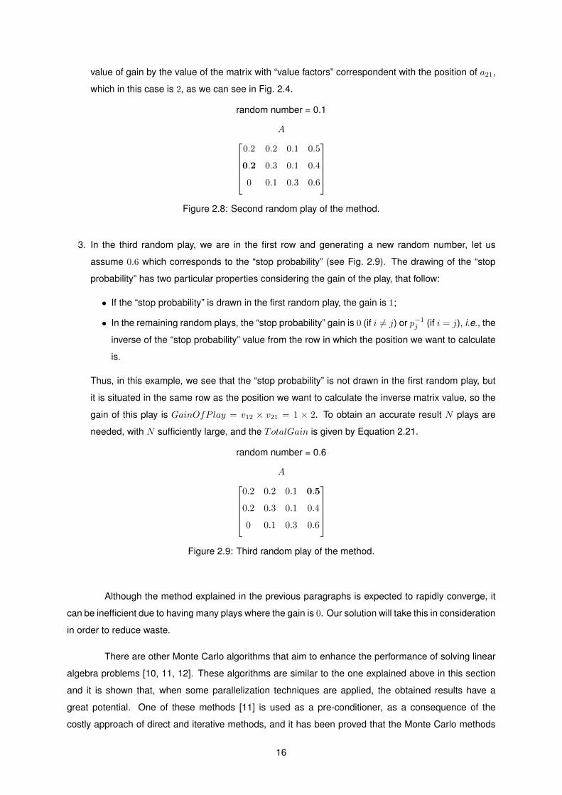
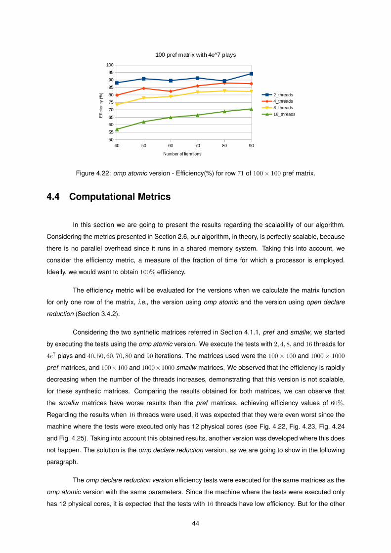
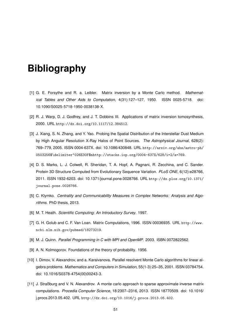

[25] The university of florida sparse matrix collection httpswwwciseufleduresearchsparse
matricesGleichindexhtml Accessed 2015-10-09
53
54

54


