Monte Carlo and quasi-Monte Carlo methods - PKUdsec.pku.edu.cn/~tieli/notes/numer_anal/MCQMC_Caflisch.pdf · MONTE CARLO AND QUASI-MONTE CARLO 3 quasi-random points converges more

Ada Numerica (1998), pp. 1-49 © Cambridge University Press, 1998

Monte Carlo and quasi-Monte Carlomethods

Russel E. Caflisch*Mathematics Department, UCLA,

Los Angeles, CA 90095-1555, USAE-mail: [email protected]

Monte Carlo is one of the most versatile and widely used numerical methods.Its convergence rate, O(N~1^2), is independent of dimension, which showsMonte Carlo to be very robust but also slow. This article presents an intro-duction to Monte Carlo methods for integration problems, including conver-gence theory, sampling methods and variance reduction techniques. Acceler-ated convergence for Monte Carlo quadrature is attained using quasi-random(also called low-discrepancy) sequences, which are a deterministic alternativeto random or pseudo-random sequences. The points in a quasi-random se-quence are correlated to provide greater uniformity. The resulting quadraturemethod, called quasi-Monte Carlo, has a convergence rate of approximatelyO((log N^N'1). For quasi-Monte Carlo, both theoretical error estimates andpractical limitations are presented. Although the emphasis in this article ison integration, Monte Carlo simulation of rarefied gas dynamics is also dis-cussed. In the limit of small mean free path (that is, the fluid dynamic limit),Monte Carlo loses its effectiveness because the collisional distance is much lessthan the fluid dynamic length scale. Computational examples are presentedthroughout the text to illustrate the theory. A number of open problems aredescribed.

Research supported in part by the Army Research Office under grant number DAAH04-95-1-0155.

R. E. CAFLISCH

CONTENTS

1 Introduction 22 Monte Carlo integration 43 Generation and sampling methods 84 Variance reduction 135 Quasi-random numbers 236 Quasi-Monte Carlo techniques 337 Monte Carlo methods for rarefied gas dynamics 42References 46

1. Introduction

Monte Carlo provides a direct method for performing simulation and integ-ration. Because it is simple and direct, Monte Carlo is easy to use. It isalso robust, since its accuracy depends on only the crudest measure of thecomplexity of the problem. For example, Monte Carlo integration convergesat a rate O{N~1/2) that is independent of the dimension of the integral.For this reason, Monte Carlo is the only viable method for a wide range ofhigh-dimensional problems, ranging from atomic physics to finance.

The price for its robustness is that Monte Carlo can be extremely slow.The order O(N~1^2) convergence rate is decelerating, since an additionalfactor of 4 increase in computational effort only provides an additional factorof 2 improvement in accuracy. The result of this combination of ease of use,wide range of applicability and slow convergence is that an enormous amountof computer time is spent on Monte Carlo computations.

This represents a great opportunity for researchers in computational sci-ence. Even modest improvements in the Monte Carlo method can havesubstantial impact on the efficiency and range of applicability for MonteCarlo methods. Indeed, much of the effort in the development of MonteCarlo has been in construction of variance reduction methods which speedup the computation. A description of some of the most common variancereduction methods is given in Section 4.

Variance reduction methods accelerate the convergence rate by reducingthe constant in front of the O(N~1/2) for Monte Carlo methods using ran-dom or pseudo-random sequences. An alternative approach to accelerationis to change the choice of sequence. Quasi-Monte Carlo methods use quasi-random (also known as low-discrepancy) sequences instead of random orpseudo-random. Unlike pseudo-random sequences, quasi-random sequencesdo not attempt to imitate the behaviour of random sequences. Instead, theelements of a quasi-random sequence are correlated to make them more uni-form than random sequences. For this reason, Monte Carlo integration using

MONTE CARLO AND QUASI-MONTE CARLO 3

quasi-random points converges more rapidly, at a rate O(N~1 (log N)k), forsome constant k. Quasi-random sequences are described in Sections 5 and 6.

In spite of their importance in applications, Monte Carlo methods re-ceive relatively little attention from numerical analysts and applied math-ematicians. Instead, it is number theorists and statisticians who design thepseudo-random, quasi-random and other types of sequence that are usedin Monte Carlo, while the innovations in Monte Carlo techniques are de-veloped mainly by practitioners, including physicists, systems engineers andstatisticians.

The reasons for the near neglect of Monte Carlo in numerical analysis andapplied mathematics are related to its robustness. First, Monte Carlo meth-ods require less sophisticated mathematics than other numerical methods.Finite difference and finite element methods, for example, require carefulmathematical analysis because of possible stability problems, but stabilityis not an issue for Monte Carlo. Instead, Monte Carlo nearly always givesan answer that is qualitatively correct, but acceleration (error reduction)is always needed. Second, Monte Carlo methods are often phrased in non-mathematical terms. In rarefied gas dynamics, for example, Monte Carloallows for direct simulation of the dynamics of the gas of particles, as de-scribed in Section 7. Finally, it is often difficult to obtain definitive results onMonte Carlo, because of the random noise. Thus computational improve-ments often come more from experience than from a particular insightfulcalculation.

This article is intended to provide an introduction to Monte Carlo methodsfor numerical analysts and applied mathematicians. In spite of the reasonscited above, there are ample opportunities for this community to make sig-nificant contributions to Monte Carlo. First of all, any improvements canhave a big impact, because of the prevalence of Monte Carlo computations.Second, the methodology of numerical analysis and applied mathematics,including well controlled computational experiments on canonical problems,is needed for Monte Carlo. Finally, there are some outstanding problemson which a numerical analysis or applied mathematics viewpoint is clearlyneeded; for example:

• design of Monte Carlo simulation for transport problems in the diffusionlimit (Section 7)

• formulation of a quasi-Monte Carlo method for the Metropolis al-gorithm (Section 6)

• explanation of why quasi-Monte Carlo behaves like standard MonteCarlo when the dimension is large and the number of simulation is ofmoderate size (Section 6).

Some older, but still very good, general references on Monte Carlo are Kalosand Whitlock (1986) and Hammersley and Handscomb (1965).

4 R. E. CAFLISCH

The focus of this article is on Monte Carlo for integration problems. Integ-ration problems are simply stated, but they can be extremely challenging.In addition, integration problems contain most of the difficulties that arefound in more general Monte Carlo computations, such as simulation andoptimization.

The next section formulates the Monte Carlo method for integration anddescribes its convergence. Section 3 describes random number generatorsand sampling methods. Variance reduction methods are discussed in Sec-tion 4 and quasi-Monte Carlo methods in Section 5. Effective use of quasi-Monte Carlo requires some modification of standard Monte Carlo techniques,as described in Section 6. Monte Carlo methods for rarefied gas dynamicsare described in Section 7, with emphasis on the loss of effectiveness forMonte Carlo in the fluid dynamic limit.

2. Monte Carlo integration

The integral of a Lebesgue integrable function f(x) can be expressed as theaverage or expectation of the function / evaluated at a random location.Consider an integral on the one-dimensional unit interval

nn= f1 f(x)dx = f. (2.i)Jo

Let a; be a random variable that is uniformly distributed on the unit interval.Then

I[f] = E[f(x)]. (2.2)For an integral on the unit cube Id = [0, l]d in d dimensions,

)dx, (2.3)

in which a; is a uniformly distributed vector in the unit cube.The Monte Carlo quadrature formula is based on the probabilistic inter-

pretation of an integral. Consider a sequence {xn} sampled from the uniformdistribution. Then an empirical approximation to the expectation is

M/] = ^ £ / ( * n ) . (2.4)n=l

According to the Strong Law of Large Numbers (Feller 1971), this approx-imation is convergent with probability one; that is,

(2.5)

In addition, it is unbiased, which means that the average of Iff [/] is exactly/[/] for any N; that is,

E[IN[f]] = I[f], (2.6)

MONTE CARLO AND QUASI-MONTE CARLO

in which the average is over the choice of the points {xn}.In general, define the Monte Carlo integration error

(2.7)

so that the bias is .E[ejv[/]] and the root mean square error (RMSE) is

£ M / ] 2 ] 1 / 2 . (2.8)

2.1. Accuracy of Monte Carlo

The Central Limit Theorem (CLT) (Feller 1971) describes the size and stat-istical properties of Monte Carlo integration errors.

Theorem 2.1 For N large,

eN[f] « aN-l'2u (2.9)

in which v is a standard normal (N(0,1)) random variable and the constanta = a[f] is the square root of the variance of / ; that is,

O f \ 1 / 2

'id(f(x)-I[f])2dxJ . (2.10)A more precise statement is that

lim Prob I a < eN <b\ = Prob(a < v < b)N—>oo \ a I

= fh{2n)-1'2e-x2l2dx. (2.11)Ja

This says that the error in Monte Carlo integration is of size O{N~1/2)with a constant that is just the variance of the integrand / . Moreover,the statistical distribution of the error is approximately a normal randomvariable. In contrast to the usual results of numerical analysis, this is aprobabilistic result. It does not provide an absolute upper bound on theerror; rather it says that the error is of a certain size with some probability.On the other hand, this result is an equality, so that the bounds it providesare tight. The use of this result will be discussed at the end of this section.

Now we present a partial proof of the Central Limit Theorem, whichproves that the error size is O(7V~1//2). Derivation of the Gaussian dis-tribution for the error is more difficult (Feller 1971). First define & =a~1(f(x{) — / ) for Xi uniformly distributed. Then

= 0,

= ja-2(f(Xi)-f-)2dx = l,

= 0 if M 3- (2.12)

R. E. CAPLISCH

The last equality is due to the independence of theNow consider the sum

N

(2.13)

Its variance is

- JV"1 I EN

L i = l

•'{£-}

+ E

1/2

N1/2

(2.14)

Therefore

E[e2N] = aN-1/2, (2.15)

which shows that the RMSE is of size O(uN~1/2).The converse of the Central Limit Theorem is useful for determining the

size of N required for a particular computation. Since the error boundfrom the CLT is probabilistic, the precision of the Monte Carlo integrationmethod can only be ensured within some confidence level. To ensure anerror of size at most e with confidence level c requires the number of samplepoints N to be

AT = e -V s(c), (2.16)

in which s is the confidence function for a normal variable; that is,

= rJ- {c)

= evi(s(c)/V2). (2.17)

For example, 95 per cent confidence in the error size requires that s = 2,approximately.

In an application, the exact value of the variance is unknown (it is asdifficult to compute as the integral itself), so the formula (2.16) cannot bedirectly used. There is an easy way around this, which is to determine theempirical error and variance (Hogg and Craig 1995). Perform M computa-tions using independent points Xi for 1 < i < MN. For each j obtain values

MONTE CARLO AND QUASI-MONTE CARLO

n for 1 < j < M. The empirical RMSE is then ejy, given by

M 2 \ l'2

( g ) )( g ) (2.18)

in whichM

IN = M-lY.IN)- (2-19)

The empirical variance is a given by

a = A^1/2eiv. (2.20)

This value can be used for a in (2.16) to determine the value of N for agiven precision level e and a given confidence level c.

2.2. Comparison to grid-based methods

Most people who see Monte Carlo for the first time are surprised that it isa viable method. How can a random array be better than a grid? Thereare several ways to answer this question. First, compare the convergencerate of Monte Carlo with that of a grid-based integration method such asSimpson's rule. The convergence rate for grid-based quadrature is O(N~k/d)for an order k method in dimension d, since the grid with N points in the unitcube has spacing N~1^d. On the other hand, the Monte Carlo convergencerate is O(N~1^2) independent of dimension. So Monte Carlo beats a grid inhigh-dimension d, if

k/d < 1/2. (2.21)

On the other hand, for an analytic function on a periodic domain, thevalue of k is infinite, so that this simple explanation fails. A more realisticexplanation for the robustness of Monte Carlo is that it is practically im-possible to lay down a grid in high dimension. The simplest cubic grid in ddimensions requires at least 2d points. For d = 20, which is not particularlylarge, this requires more than a million points. Moreover, it is practicallyimpossible to refine a grid in a high dimension, since a refinement requiresincreasing the number of points by factor 2d. In contrast to these difficultiesfor a grid in high dimension, the accuracy of Monte Carlo quadrature isnearly independent of dimension and each additional point added to theMonte Carlo quadrature formula provides an incremental improvement inits accuracy. To be sure, the value of N at which the O(N^1^2) error estim-ate becomes valid (that is, the length of the transient) is difficult to predict,but experience shows that, for problems of moderate complexity in mod-erate dimension (for instance d = 20), the 0{N~1/2) error size is typicallyattained for moderate values of N.

8 R. E. CAFLISCH

Two additional interpretations of Monte Carlo quadrature are worthwhile.Consider the Fourier representation of a periodic function with period one

/(*)= £ /»e 2 ^ . (2.22)k=—oo

The integral /[/] is just /(0); that is, the contributions to the integral are0 from all wave-numbers k ^ 0. For a grid of spacing 1/n, the grid-basedquadrature formula is

i n ) . (2.23)

The contributions to this sum are 0 (as they should be) from wave-numbersk 7 mn for some integer m, and the contributions are f(k) for wave-numbersk = mn. That is, the accuracy of grid-based quadrature is 100 per cent fork T mn, but 0 per cent for k = mn (with mÔ) . Monte Carlo quadratureusing a random array is partially accurate for all k, which is superior to agrid-based method if the Fourier coefficients decay slowly.

Finally, insight into the relative performance of grid-based and MonteCarlo methods is gained by considering the points themselves in a highdimension. For a regular grid, the change from one point to the next isonly a variation of one component at a time, that is, (0,0,... , 0,0) H->(0,0,... ,0,1/n). In many problems, this is an inefficient use of the un-varied components. In a random array, all components are varied in eachpoint, so that the state space is sampled more fully. This accords well withthe global nature of Monte Carlo: each point of a Monte Carlo integrationformula is an estimate of the integral over the entire domain.

3. Generation and sampling methods

3.1. Random number generators

The numbers generated by computers are not random, but pseudo-random,which means that they are made to have many of the properties of ran-dom number sequences (Niederreiter 1992). While this is a well-developedsubject, occasional problems still occur, mostly with very long sequences(N > 109). The methods used to generate pseudo-random numbers aremostly linear congruential methods. There is a series of reliable pseudo-random number generators in the popular book Numerical Recipes (Press,Teukolsky, Vettering and Flannery 1992). It is important to use the routinesranO, rani, ran2, ranS, ran4 from the second edition (for instance, rani isrecommended for N < 108); the routines RANO, RANI, RAN2, RANS from.the first edition of this book had some deficiencies (see Press and Teukolsky(1992)).


For very large problems requiring extremely large values of N (as high as1013!), reliable sequences can be obtained from the project Scalable ParallelRandom Number Generators Library for Parallel Monte Carlo Computa-tions (http://www.ncsa.uiuc.edu/Apps/SPRNG/).

3.2. Sampling methods

Standard (pseudo-) random number generators produce uniformly distrib-uted variables. Non-uniform variables can be sampled through transforma-tion of uniform variables. For a non-uniform random variable with densityp(x), the expectation of a function f(x) is

= Jf(x)p(x)dx. (3.1)

For a sequence of random numbers {xn} distributed according to the densityp, the empirical approximation to the expectation is

W ] = E/(*n) (3-2)

and the resulting quadrature error is

eN[f] = I[f}-lN[f}. (3.3)

As in the one-dimensional case, the Central Limit Theorem says that

eN[f] ~ N-ôv (3.4)

in which v is -/V(0,1) and

a2 = j{f-f)2p{x)dx. (3.5)

Next we discuss methods for generating non-uniform random variablesstarting from uniform random variables.

3.3. Transformation method

This is a general method for producing a random variable x with densityp(x), through transformation of a uniform random variable. Let y be auniform variable and look for a function X(y), so that x — X(y) has thedesired density p(x).

Define the cumulative distribution function

P(x) = fX p(x') dx'. (3.6)• /—oo

Determination of the mapping X(y) is through the following computationof the expectation. For any function / ,

Ep[f(x)} = EaDi{[f(X(y))}, (3.7)

10 R. E. CAFLISCH

so that, using a change of variables,

J f(x)p(x)dx = J f(X(y))dy

= J f{x){dy/dx)dx. (3.8)

This implies that p(x) = dy/ dx = 1/X'(y) so that / (y' p(x)dx = y; i.e.,

P(X(y)) = yX(y) = P~\y). (3.9)

This formulation is convenient and explicit but not necessarily easy to im-plement, as it may be difficult to compute the inverse of the function P.

3.4- Gaussian random variables

As an example of the transformation method, a Gaussian (normal) randomvariable has density p and cumulative distribution function P given by

p{x) =

rJ-

= i + \ erf (x/V2), (3.10)

in which erf is the error function defined by

erf(z) = - = / e-t2dt. (3.11)V71" Jo

One way to sample from a Gaussian distribution is to apply the inverseof the Gaussian cumulative distribution function P to a uniform randomvariable y. Sample a normal variable x, starting from a uniform variable y,by

y = P(x) = ± + ±eTf(x/V2), (3.12)

that is,

x = v /2erf~1(2j/- l) . (3.13)

Approximate formulas for P^~1\y) or erf"1 are found in Kennedy andGentle (1980).

For the Gaussian distribution, as well as for a number of other distribu-tions, special transformations are a useful alternative to the general trans-formation method. The simplest of these is the Box-Muller method. Itprovides a direct way of generating normal random variables without in-verting the error function. Starting with two uniform variables y\,y2, two


normal variables £i,£2 are obtained by

= ^/-21og(yi)cos(27n/2),

x2 = ^/-21og(yi)ain(27ry2). (3.14)

Box-Muller is based on the following observation. First change from rect-angular to polar coordinates, that is,

(x\,X2) = (r cos 0,r sin 9), (3.15)

so that

dxidx2 = rdrd9. (3.16)

The corresponding transformation of the probability density function is

(27r)-1e-(xi+x2)/2 dxi dx2 = (2Tr)'1e'r2/2r dr 66. (3.17)

This shows that the angular variable y\ = 9/(2ir) is uniformly distributedover the unit interval. Next the variable r is easily sampled, since it hasdensity re~r I2 and corresponding cumulative distribution function

P(r) = f e"r'2/V dr' = 1 - e~^2. (3.18)Jo

Therefore r can be sampled by

^ ^ ) . (3.19)

After replacing 3/2 by 1 — 3/2, the resulting transform

(VUV2) ^ {r,0)-* {xi,x2) (3.20)

is given in (3.14).The only disadvantages of the Box-Muller method are that it requires

evaluation of transcendental functions and that it generates two randomvariables when only one may be needed. See Marsaglia (1991) for examplesof efficient use of Box-Muller.

3.5. Acceptance-rejection method

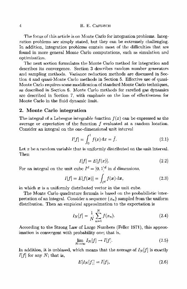
Another general way of producing random variables from a given densityp(x) is based on a probabilistic approach. This method shows the powerand flexibility of stochastic methods. For a given density function p(x),suppose that we know a function q(x) satisfying

q(x)>p(x), (3.21)

and that we have a way to sample from the probability density

q{x) = q(x)/I[q], (3.22)

12 R. E. CAFLISCH

0.1 0.2 0.3 0.4 0.5 0.6 0.7 0.8 0.9 1

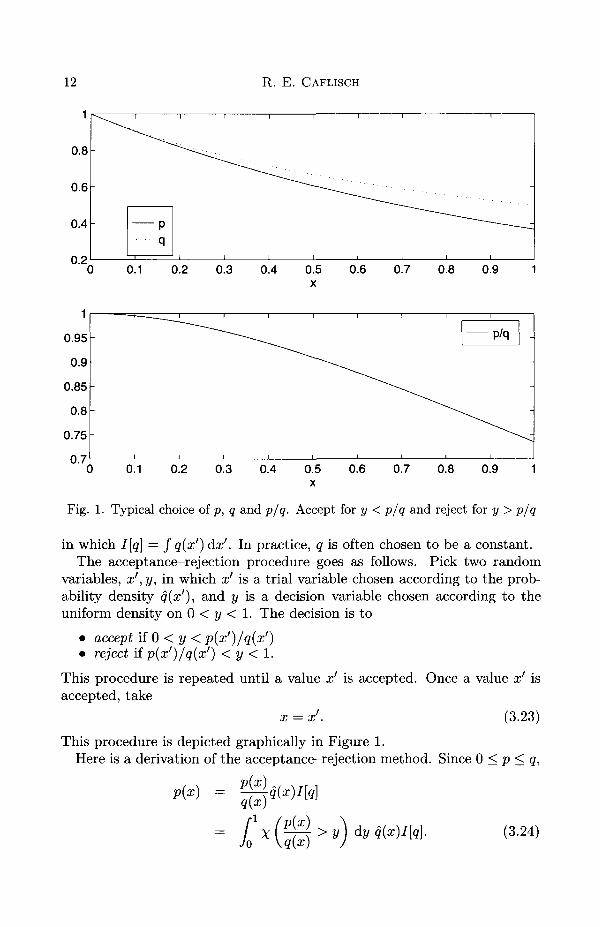
Fig. 1. Typical choice of p, q and p/q. Accept for y < p/q and reject for y > p/q

in which I[q] = J q(x') dx'. In practice, q is often chosen to be a constant.The acceptance—rejection procedure goes as follows. Pick two random

variables, x', y, in which x' is a trial variable chosen according to the prob-ability density q(x'), and y is a decision variable chosen according to theuniform density on 0 < y < 1. The decision is to

• accept if 0 < y < p(x')/q(x')• reject if p(x')/q(x') < y < 1.

This procedure is repeated until a value x' is accepted. Once a value x' isaccepted, take

x = x'. (3.23)

This procedure is depicted graphically in Figure 1.Here is a derivation of the acceptance-rejection method. Since 0 < p < q,

p(x) =q(x)

(3.24)


So,

Jf(x)p(x)dx = J jT1 f(x)X(^>y)q(x)dydxI[q]

f{<) i[q\p(x'n)/q(x'n)>yn

« TV"1 X ! /(*")> (3-25)accepted pts

in which

A7"' = total number of trial points,

N = total number of accepted points

« N'/I[q]. (3.26)

The acceptance-rejection method has some obvious advantages that oftenmake it the method of choice for generating random variables with a givendistribution. It does not require inversion of the cumulative distributionfunction P. In addition, it works even if the density function p has not beennormalized to have integral 1. One disadvantage of the method is that itmay be inefficient, requiring many trials before acceptance. In practice thisis often not a serious deficiency, since the largest share of the computationis on the integrand rather than on the random point selection.

An extension of the acceptance—rejection method called the Metropolisalgorithm (Kalos and Whitlock 1986) is used to find the equilibrium distri-bution for a stochastic process.

4. Variance reduction

In Monte Carlo integration, the error e and the number N of samples arerelated by

e = O (aN'l/2) , (4.1)

N = O(a/e)2. (4.2)

The computational time required for the method is proportional to thesample number N and thus is of size O(a/e)2, which shows that compu-tational time grows rapidly as the desired accuracy is tightened. There aretwo options for acceleration (error reduction) of Monte Carlo. The first isvariance reduction, in which the integrand is transformed in a way that re-duces the constant variance a. The second is to modify the statistics, that is,to replace the random variables by an alternative sequence which improvesthe exponent 1/2. In this section, various strategies for variance reductionare described. In Section 5, we discuss quasi-random variables, an example

14 R. E. CAFLISCH

of the second approach. One note of caution is that the acceleration meth-ods described here may require extra computational time, which must bebalanced against savings gained by reduced N. In most examples, however,the savings due to variance reduction are quite significant.

4-1. Antithetic variables

Antithetic variables is one of the simplest and most widely used variancereduction methods. The method is as follows: for each (multi-dimensional)sample value x, also use the value — x. The resulting Monte Carlo quadrat-ure rule is

n) + f(-Xn)}. (4.3)7 1 = 1

For example, the vector x could be the discrete states in a random walk, sothat the dimension would be the number of time-steps in the walk. Whenantithetic variables are used for a problem involving a random walk, thenfor each path x = (x\,..., x^), we also use the path —x = (—x\,..., — x^).

The use of antithetic variables is motivated by an expansion for smallvalues of the variance. Consider, for example, the expectation E[f(x)] inwhich x is an JV(O, <r2) random variable with a small. Set

x — ax. (4-4)

The Taylor expansion of / = f(crx) (for small a) is

x + O(a2). (4.5)

Since the distribution of x is symmetric about 0, the average E[x] of thelinear term is zero. In a standard Monte Carlo integral of / , these terms donot cancel exactly, so that the Monte Carlo error is proportional to a. Withantithetic variables, on the other hand, the linear terms cancel exactly, sothat the remaining error is proportional to a2.

4-2. Control variates

The idea of control variates is to use an integrand g, which is similar to /and for which the integral I[g] = f g(x)dx is known. The integral /[/] isthen written as

j f{x) dx = J (f(x) - g(x)) dx + J g{x) dx. (4.6)

Monte Carlo quadrature is used on the integral of / — g to obtain the formula

7«[/] = Jj E (/(*") - 9(xn)) + I[9}. (4.7)n=l


The resulting integration error ejv[/] = /[ / ] — IN[I] is of size

eN[f] « aj-gN-1'2, (4.8)

in which the relevant variance is

°3f-g = J{fc)-9(x))2<te (4-9)

using the notation

f{x) = f{x) - /[ /] , g(x) = gix) - I[g}. (4.10)

This shows that the control variate method is effective if

CTf-g < Of. (4.11)

Optimal use of a control variate is made by introducing a multiplier A.For a given function g, write the integral of / as

j fix) dx = f ifix) - Xg(x)) dx + A J gix) dx. (4.12)

The error in Monte Carlo quadrature of the first integral is proportional tothe variance

dx. (4.13)

The optimal value of A is found by minimizing <7/_Ag t ° obtain

A = E[fg]/E[g2]

( y > ) (4.14)

4-3. Matching moments method

Monte Carlo integration error is partly due to statistical sampling error, thatis, differences between the desired density function p(x) and the empiricaldensity function of the sampled points {xn}^=1. Part of this difference canbe seen directly through comparison of the moments of the two distributions.Define the first and second moments mi and 7712 of p as

77ii = / xp{x) dx, 7712 = / x2pix)dx. (4-15)

The first and second moments Mi and M2 of the sample {xn}^=1 are

N N

Ml = N~l ^ xn, M2 = A ^ 1 y ^ x2 (4-16)n=l n=l

The moment error is due to the inequality of these moments, that is,

Ml 7^ m i > M2 7^ rn2- (4-17)

16 R. E. CAFLISCH

A partial correction to the statistical sampling error is to make the mo-ments exactly match. This can be done by a simple transformation of thesample points. To match the first moment of the sample with that of p,replace xn by

yn = (xn-fJ'i) + m1. (4.18)

This satisfieslYn = mi (4.19)

so that the first moment is exactly right. To match the first two moments,replace xn by

\Vtl2 771? . ,Vn = (xn- mj/c + mi, c=J f. (4.20)

V M - Mi

Then

N-1Y,Vn = ml, N-1'£i& = rn2. (4.21)These transformed sequences with the correct moments must be used with

some caution. Since the transformation involves Hi and ^2, the new samplepoints yn are no longer independent, and Monte Carlo error estimates are notso straightforward. For example, the Central Limit Theorem is not directlyapplicable, and the method may be biased. Actually, this is an example ofthe second approach to acceleration of Monte Carlo, through modificationof the properties of the random sequence. It is presented here along withvariance reduction methods, however, because the resulting improvementin Monte Carlo accuracy is comparable to that gained through variancereduction.

Pullin (1979) has formulated a method in which the sample points areindependent and have a prescribed empirical mean and variance, but comefrom a Gaussian distribution with a randomly chosen mean and variance.

4-4- Stratification

Stratification combines the benefits of a grid with those of random variables.In the simplest case, stratification is based on a regular grid with uniformdensity in one dimension. Split the integration region fi = [0,1] into Mpieces Q/- given by

[W]Then, each subset has the same measure, |fifc| = 1/M. Define the averagesover each fi^ by

/ » = fk = l^fcl"1 / f(x) dx for x € nk. (4.23)


For each k, sample Nk = N/M points {x\ '} uniformly distributed in fife.Then the stratified quadrature formula is just the sum of the quadraturesover each subset, that is,

M N/M

IN = iV-1 £ £ / (*!fc)) • (4.24)fc=l i = l

The Monte Carlo quadrature error for this stratified sum is

°l = I (f(x) - f(x)f dxM f

— 2_j I \J\XI Jk) ax- {^•zo)

For this stratified quadrature rule, there is a simple result. StratifiedMonte Carlo quadrature always beats the unstratified quadrature, since

as < a. (4.26)

The proof of this inequality is straightforward. For each k, c = fk is theminimizer of

jf (f(x) - c)2 dx. (4.27)

In particular,

/ (f(x)-fk)2dx<[ (f(x)-f)2dx. (4.28)

Add this over all A; to getM

dx°l = TtLdx

= a2. (4.29)

Stratification can be phrased more generally as follows. Split the integra-tion region f2 into M pieces fife with

n = ujf=1nk. (4.30)

Take Nk random variables in each piece fife with

M

Y^Nk = N. (4.31)fc=i

18 R. E. CAFLISCH

In each subset £lk choose points xi distributed with density p^ (x) in which

x) = p(x)/pk,

Pk = [ p(x)dx. (4.32)

The stratified quadrature formula is the following sum over k:

M - Nk

M/] = £ f £/«)• (4.33)fc=l i V f c n = l

The resulting integration error is

eN[f] = I[f]-IN[f]M

= £$[/]• (4-34)fc=i

The components of this error are

(4.35)

in which the variances are

O r \ V2

' (f(x)- f^)2v(-k)(x)dx)nk )

1/2(4.36)

\JUk /

and the averages arefk= ! f(x)p(x)dx/pk. (4.37)

Jnk

Stratification always lowers the integration error if the distribution ofpoints is balanced. The balance condition is that, for all k,

pk/Nk = 1/N, (4.38)

that is, the number of points in set Clk is proportional to its weighted sizepk- The resulting error for stratified quadrature is

(fc)2. (4.39)

Since the variance over a subset is always less than the variance over thewhole set, that is,

as < a, (4.40)


then stratification always lowers the integration error. Actually, a betterchoice than the balance condition may be to put more points where / haslargest variation. An adaptive method for stratification was formulated byLepage (1978) and is described by Press et al. (1992).

4-5. Importance sampling

Importance sampling is probably the most widely used Monte Carlo variancereduction method. Consider the simple integral / f(x) dx and rewrite it byintroducing a density p as

nn =

Now think of this as an integral with density function p. Sample points xn

from the density p{x) and form the Monte Carlo estimate

The resulting error epj[f} = I[f] — IN[I} has size

eN[f] « apN-1'2, (4.43)

in which the variance av is

So importance sampling will reduce the Monte Carlo quadrature error, if

Op <C u. (4.45)

Importance sampling is an effective method when f/p is nearly constant,so that Up is small. One difficulty in this method is that sampling from thedensity p is required, but this can be performed using acceptance-rejection,if necessary. One use of importance sampling is to emphasize rare but im-portant events, i.e., small regions of space in which the integrand / is large.

4-6. Russian roulette

Some Monte Carlo computations involve infinite sums, for instance, due toiteration of an integral equation. The Russian roulette method converts aninfinite sum into a sum that is of finite length for each sample. Consider thesum

oo

S = Y, an (4-46)n=0

20 R. E. CAFLISCH

and suppose that the terms an are exponentially decreasing, that is,

an\ < c\n, (4.47)

in which 0 < A < 1. Choose A < K < 1, and let M be chosen according to adiscrete exponential distribution, so that

Prob(M > n) = Kn. (4.48)

Define the random sumM

S=J2 K~n<1n- (4-49)n=0

Since |K~nan| < (A/K)™ and |A/K| < 1, then this sum is uniformly boundedfor all M. Then

oo

E[S] = Yl Prc-b(M > n)K-nann=0

= S. (4.50)

This formula leads to the following Monte Carlo method for computationof the infinite sum (4.46):

N Mi

SN = iv-1 E E K~na^ (4-51)i=0 n=0

in which the values Mj are chosen according to the probability distribution(4.48). In this method, the terms an could also be computed by a MonteCarlo integral.

4-7. Example of variance reduction

As an example of the use of variance reduction consider the three-dimensionalGaussian integral

I[u\ = (2TT)-3/2 r f°° [°° mr^+^+^dzidzadzs, (4.52)J—oo J—oo J—oo

in which the integrand u is defined by

u = (l + ro)-1a + ri)-1(l + r2)-

1(l + r3)-1,

r i = ™'-*2/2

r2 =

r3 = r2eax*-a2/2. (4.53)

This integral can be interpreted as the present value of a payment of $1 fouryears from now, for an interest rate of r» in year i. The interest rates are


allowed to evolve according to a lognormal model with variance a, that is,

n = ri-1eaXi-a2/2, (4.54)

in which the x[s are independent N(0,1) Gaussian random variables. Thefactors (1 + n)" 1 are the discount factors. For the computations below, wetake r0 = 0.10 and a = 0.1.

We evaluate I[u] by sampling X{ from an N(0,1) distribution using thetransformation method, that is, by direct inversion of the cumulative dis-tribution function for a normal random variable. Then we apply antitheticvariables and control variates to this problem.

Approximate (1 + r,)"1 by 1 — r, for i > 1. Then form the control variateas

g = (1 + ro)"1^ - n ) ( l - r2)(l - rs). (4.55)

Since g consists of a sum of linear exponentials, its integral can be performedexactly, for instance

rJ—o

(4.56)

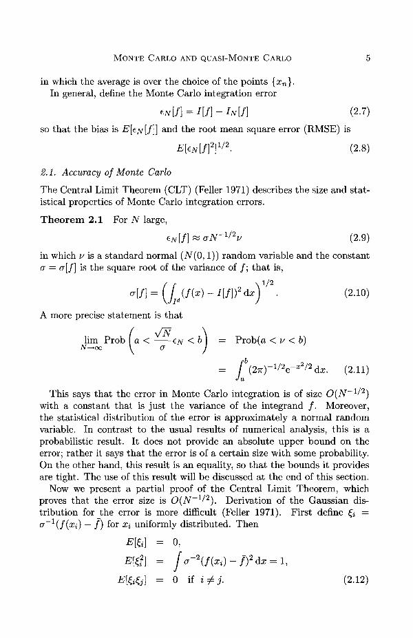
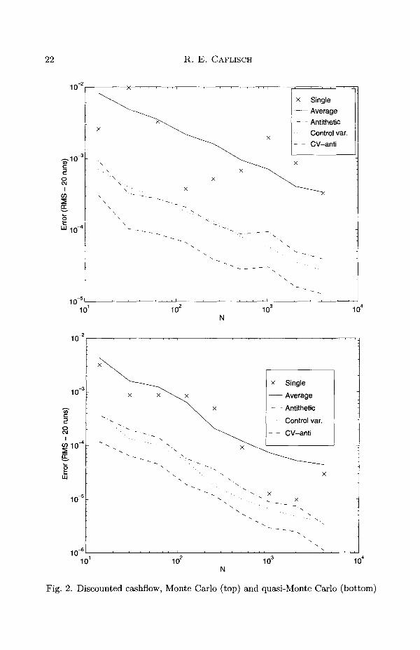
Numerical results are presented in Figure 2. This compares the quad-rature error from standard Monte Carlo, antithetic variables and controlvariates, using both standard pseudo-random points and the quasi-random(Sobol') points that will be discussed in the next section. In order to make ameaningful comparison, we have performed an average (root mean square)of the error over 20 runs for each value of N. The computations are allindependent, that is, the same random number is never used twice. Thefigure also shows the results from a single run without averaging or variancereduction. The results show the following points.

• Both control variates and antithetic variables provide significant errorreduction.

• Control variates and antithetic variables together perform better thaneither one alone. This shows that the error reduction from the twomethods are different.

• Quasi-Monte Carlo, which will be discussed in Section 5, has smallererror and a faster rate of convergence.

• Control variates and antithetic variables, both separately and together,provide further error reduction when used with quasi-Monte Carlo.

22 R. E. CAFLISCH

10

-10 -c

oCM

I

w

210 -

10"

X

\

" • \

\ • • •

\

\

\

\

X

J . 1 . 1

X

" • • " • • < v .

X

n

X

\

X

X

X

1

— I p 1 .—1 1—1—1—1

x Single :AverageAntitheticControl var.

- - CV-anti

x :•

•

10' 10° 10'

10"

10" -

IoCM

i

LU

10" -

10

1 1 1 1 1 1—I—r-| 1 1 1 1 1 1—i—r

\ ^ X

" - _ X

X " . ' " • * .

X ~^

X X

x "Sl

X

- j 1 1 1 1 1 i I r-_

x Single

Average

- - Antithetic

Control var.

- - CV-anti

:

:

-

^ ^

X

X-. x -

• • • - . . . ~ x . ^ :

' • • s ;

10' 10' 10" 10'

Fig. 2. Discounted cashflow, Monte Carlo (top) and quasi-Monte Carlo (bottom)


5. Quasi-random numbers

Quasi-random sequences are a deterministic alternative to random or pseudo-random sequences (Kuipers and Niederreiter 1974, Hua and Wang 1981,Niederreiter 1992, Zaremba 1968). In contrast to pseudo-random sequences,which try to mimic the properties of random sequences, quasi-random se-quences are designed to provide better uniformity than a random sequence,and hence faster convergence for quadrature formulas. Uniformity of a se-quence is measured in terms of its discrepancy, which is defined in Sec-tion 5.2 below, and for this reason quasi-random sequences are also calledlow-discrepancy sequences. Some have objected to the name quasi-random,since these sequences are intentionally not random. We continue to use thisname, however, because of the unpredictability of quasi-random sequences.

5.1. Monte Carlo versus quasi-Monte Carlo

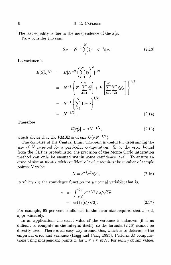
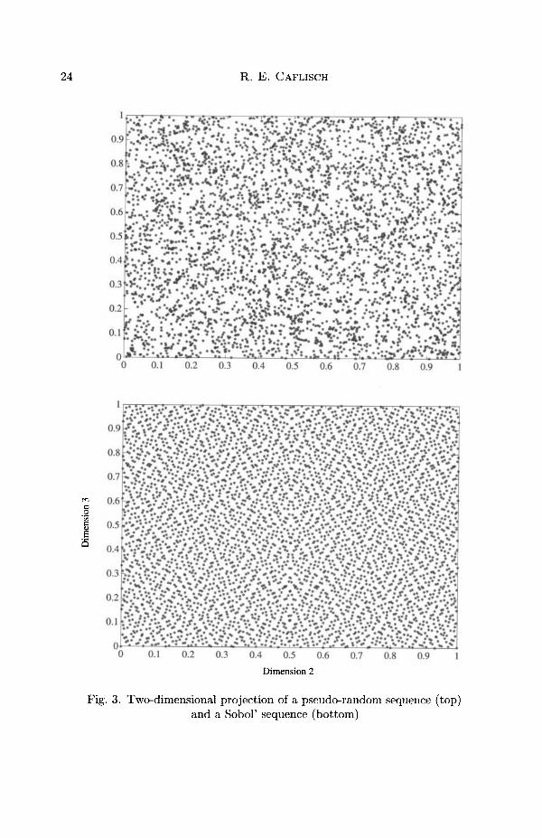
The difference between standard Monte Carlo and quasi-Monte Carlo is bestillustrated by Figure 3, which compares a pseudo-random sequence with aquasi-random sequence (a Sobol' sequence) in two dimensions. StandardMonte Carlo methods use pseudo-random sequences and provide a conver-gence rate of (^(iV"1/2) for Monte Carlo quadrature using N samples. Inaddition to integration problems, standard Monte Carlo is applicable to op-timization and simulation problems.

The limiting factor in accuracy of standard Monte Carlo is the clumpingthat occurs in the points of a random or pseudo-random sequence. Clumpingof points, as well as spaces that have no points, is clearly seen in the pseudo-random sequence in Figure 3. The reason for this clumping is that the pointsare independent. Since different points know nothing about each other,there is some small chance that they will lie very close together. A simpleargument shows that about i/N out of TV" points lie in clumps.

Quasi-Monte Carlo methods use quasi-random sequences, which are de-terministic, with correlations between the points to eliminate clumping. Theresulting convergence rate is O((logN)kN~l). Because of the correlations,quasi-random sequences are less versatile than random or pseudo-randomsequences. They are designed for integration, rather than simulation or op-timization. On the other hand, the desired result of a simulation can oftenbe written as an expectation, which is an integral, so that quasi-Monte Carlois then applicable. As discussed below, this often introduces high dimen-sionality, which can limit the effectiveness of quasi-Monte Carlo sequences.

5.2. Discrepancy

Quasi-random sequences were invented by number theorists who were in-terested in the uniformity properties of numerical sequences (Kuipers andNiederreiter 1974, Hua and Wang 1981). An important first step is formu-

24 R. E. CAFLISCH

0.2 0.3 0.4 0.5 0.6 0.7 0.8 0.9

Fig. 3. Two-dimensional projection of a pseudo-random sequence (top)and a Sobol' sequence (bottom)


lating a quantitative measure of uniformity. Uniformity of a sequence ofpoints is measured in terms of its discrepancy.

For a sequence of iV points {xn} in the unit cube Id, define

RN( J) = ^#{xn € J} - m( J) (5.1)

for any subset J of Id. RN(J) is just the Monte Carlo quadrature error inmeasuring the volume of J. The discrepancy is then defined by some normapplied to Rj^(J). First, restrict J to be a rectangular set, and define theset of all such subsets to be E. Since a rectangular set can be defined by twoantipodal vertices, a rectangle J can be identified as J = J(x, y) in whichthe points x and y are antipodal vertices. Now define two discrepancies:DN, which is an L°° norm on J, and T/v, which is an 1? norm, defined by

DN =J€E

TN = f RN(J{x,y))2 dxJ(x,y)£l2d,xi<yi

dy (5.2)

It is useful to also define the discrepancy over rectangular sets with onevertex at 0, as

D*N = sup \RN(J)\JeE*

(5.3)

in which E* is the set {J(0, x)}. Other definitions include terms from lower-dimensional projections of the sequence (Hickernell 1998).

5.3. Koksma-Hlawka inequality

Quasi-random sequences are useful for integration because they lead to muchsmaller error than standard Monte Carlo quadrature. The basis for analys-ing quasi-Monte Carlo quadrature error is the Koksma-Hlawka inequality.

Consider the integral

/[/] = / /(*) dx (5.4)

and the Monte Carlo approximation

^ / ( * n ) , (5.5)

and define the quadrature error

(5.6)

26 R. E. CAFLISCH

Define the variation (in the Hardy-Krause sense) of / , a function of a singlevariable, as

V[f] = fJo dt

In d dimensions, the variation is denned as

9*f• dtd

dt. (5.7)

(5.8)

in which /} is the restriction of the function / to the boundary X{ = 1.Since these restrictions are functions of d — 1 variables, this definition isrecursive.

Theorem 5.1 (Koksma-Hlawka theorem) For any sequence {xn} andany function / with bounded variation, the integration error e is boundedas

e[f] < V[f] D*N. (5.9)

It is instructive to compare the Koksma-Hlawka result to the root meansquare error (RMSE) of standard Monte Carlo integration using a randomsequence, that is,

EW\2]l/2 = v[f]N~l/2, (5.10)

in which

°\f\ = <Kfid{f{x)-I[f])2dxY\

{x)dx-^Yjf(xn). (5.11)

In comparing the Koksma-Hlawka inequality (5.9) and the RMSE forstandard Monte Carlo integration (5.10), note the following points.

• Both error bounds are a product of one factor that depends on thesequence {i.e., DN for Koksma-Hlawka and JV"1/2 for RMSE) and afactor that depends on the function / {i.e., V[f] for Koksma-Hlawkaand a[f] for RMSE).

• The Koksma-Hlawka inequality is a worst-case bound, whereas theRMSE (5.10) is a probabilistic bound.

• The RMSE (5.10) is an equality, and so it is tight, whereas Koksma-Hlawka is an upper bound.

• Our experience is that V[f] in Koksma-Hlawka is usually a gross over-estimate, while the discrepancy is indicative of actual performance.


A further, more subtle point is that for standard Monte Carlo each point isan estimate of the entire integral. A typical quasi-random sequence, on theother hand, has a hierarchical structure, so that the initial points samplethe integrand on a coarse scale and later points sample it on a finer scale.This is the source of the log N terms in the discrepancy bounds cited below.

5.4- Proof of the Koksma-Hlawka inequality

First consider functions / that vanish on the boundary of the unit cube.Note that

N }

(5.12)1= <T-Y6(x-xn)-l\dx,

N ^n=l

in which R(x) = RN(J(0,X)) as defined in Section 5.2. Since there are noboundary terms, then

elf] =I

N

n=l

R(x)df{x)

(supi?(a;))

D*NV[f}. (5.13)

For / that is nonzero on the boundary of the unit cube, the terms fromintegration by parts are bounded by the boundary terms in V[/].

5.5. Average integration error

Most computational experience confirms that discrepancy is a good indicatorof quasi-Monte Carlo performance, while variation is not a typical indicator.In 1990, Wozniakowski (Wozniakowski 1991) proved the following surprisingresult.

Theorem 5.2 We have

(5.14)

in which the expectation E is taken with respect to functions / distributedaccording to the Brownian sheet measure.

28 R. E. CAFLISCH

The Brownian sheet measure is a measure on function space. It is a naturalgeneralization of simple Brownian motion b(x) to multi-dimensional 'time'x. With probability one, a function f(x), chosen from the Brownian sheetmeasure, is approximately 'half-differentiable'. In particular, its variation isinfinite. In this context, we can definitely say that variation is not a goodindicator of integration error. Since Wozniakowski's identity (5.14) is anequality, it follows that the I? discrepancy Tjy does agree with the typicalsize of quasi-Monte Carlo integration error. Our computational experienceis that Tjy and DN are usually of the same size.

Denote x' = {x'^)f=1 in which x\ = 1 — Xi\ also denote the finite differenceoperator Dif(x') = f (x'+Aii'j)—f (x'), in which e is the ith coordinate vec-tor. The Brownian sheet is based at the point x' = 0, that is, x = ( 1 , . . . , 1),and has f(x' = 0) = / ( I , . . . , 1) = 0. For any point x' in /dand any setof positive lengths Aj (with x\ + Aj < 1), the multi-dimensional differenceD\ ... Ddf(x) is a normally distributed random variable with mean zero andvariance

E[(D1... Ddf{x)f] = Ax . . . Ad. (5.15)

This implies that

E[ df(x) df(y)} = 6(x - y) dx dy, (5.16)

in which d/ is understood in the sense of the Ito calculus (Karatzas andShreve 1991). Moreover f(x') = 0 if x\ = 0 for any i. For any x in Id, f(x)is normally distributed with mean zero and variance

E[f(x)2} = f[x'i. (5.17)i=l

Wozniakowski's proof of (5.14) was a straightforward calculation of bothsides of the equality. The following proof, derived by Morokoff and Caflisch(1994), is based on the properties of the Brownian sheet measure and followsthe same lines as the proof of the Koksma-Hlawka inequality.

Proof of Wozniakowski's identity. First rewrite the integration error E[f]using integration by parts, following the steps of the proof of the Koksma-Hlawka inequality. Note that

( 1 N 1

I n=l )

in which R(x) = RN(J(0,X)) as defined in Section 5.2. Also, R(x) — 0 ifXi = 0, and f(x) = 0 if x, = 1, for any i. This implies that the boundary


terms all disappear in the following integration by parts:N

e\f\ = //w*~E/w

fJid R(x)df(x)

The quantity d/ in this identity is denned here through the Ito calculus,even though V[f] = 00 with probability one.

It follows from (5.16) that the average square error is

E[s[f\2} = E

[ldxld

R(x)R(y)E[df(x)df(y)}

[id

R(x)2dx

(5.19)

5.6. Quasi-random number generators

An infinite sequence {xn} is uniformly distributed if

lim DN = 0.N-*oo

(5.20)

The sequence is quasi-random if

DN < cQogAQkjV"1, (5.21)

in which c and k are constants that are independent of N, but may dependon the dimension d. In particular, it is possible to construct sequences forwhich k = d. It is also common to say that a sequence is quasi-random onlyif the exponent k is equal to the dimension d of the sequence.

The simplest example of a quasi-random sequence is the Van der Corputsequence in one dimension (d = 1) (Niederreiter 1992). It is described mostsimply as follows. Write out n in base 2. Then obtain the nth point xn byreversion of the bits of n around the decimal point, that is,

n =xn =

a m a m _i . . . aiao (base 2)• • • am-iam (base 2). (5.22)

Halton sequences (Halton 1960) are a generalization of this procedure. Inthe kth dimension, expand n in base p^, the fcth prime, and form the fcth

30 R. E. CAFLISCH

component by reversion of this expansion around the decimal point. Thediscrepancy of a Halton sequence is bounded by

£>jv(Halton) < cd(log AîV" 1 (5.23)

in which Cd is a constant depending on d. On the other hand, the averagediscrepancy of a random sequence is

E[Tl (random)]1/2 = c ^ " 1 / 2 . (5.24)

Additional sequences go by the names of Haselgrove (Haselgrove 1961),Faure (Faure 1982), Sobol' (Sobol' 1967, 1976), Niederreiter (Niederreiter1992, Xing and Niederreiter 1995), and Owen (Owen 1995, 1997, 1998, Hick-ernell 1996). Niederreiter has formulated a general theory for quasi-randomsequences in terms of (t,s) nets (Niederreiter 1992). All of these sequencessatisfy bounds like (5.23), but the more recent constructions have muchbetter constants ca-

An algorithm for construction of a Sobol' sequence is found in Press etal. (1992) and for Niederreiter sequences in Bratley, Fox and Niederreiter(1994). Various quasi-random number generators are found in the softwarecollection ACM-Toms at ht tp: / /www.net l ib .org/ toms/ index.html .

For quasi-random sequences with discrepancy of size O((log N)dN~l), theKoksma-Hlawka inequality implies that the integration error is of this samesize, that is,

e[f]<cV\f]{\ogN)dN-\ (5.25)

Note that the Koksma-Hlawka inequality applies for any sequence. Forquasi-random sequences, the discrepancy is small, so that the integrationerror is also small.

5.7. Limitations: smoothness and dimension

The Koksma-Hlawka inequality and discrepancy bounds for a quasi-randomsequence together imply that quasi-Monte Carlo quadrature converges muchfaster than standard Monte Carlo quadrature. On the other hand, there areseveral distinct limitations to the effectiveness of quasi-Monte Carlo methods(Morokoff and Caflisch 1994, 1995).

First, there is no theoretical basis for empirical estimates of accuracy ofquasi-Monte Carlo methods. Recall from Section 2 that the Central LimitTheorem can be used to test the accuracy of standard Monte Carlo quadrat-ure as the computation proceeds, and then to predict the required numberof samples N for a given accuracy level. Since there is no Central LimitTheorem for quasi-random sequences, there is no corresponding empiricalerror estimate for quasi-Monte Carlo. On the other hand, confidence inthe accuracy of quasi-Monte Carlo integration comes from refining a set ofcomputations.


Second, quasi-Monte Carlo methods are designed for integration and arenot directly applicable to simulation. This is because of the correlationsbetween the points of a quasi-random sequence. However, in many simula-tions the desired result is an expectation of some quantity, which can thenbe written as a high-dimensional integral on which quasi-Monte Carlo canbe used. In fact, we can think of the different dimensions of a quasi-randompoint as independent, so that quasi-random sequences can represent a simu-lation by allocating one dimension per time-step or decision. This approachoften requires a high-dimensional quasi-random sequence.

Third, quasi-Monte Carlo integration is found to lose its effectiveness whenthe dimension of the integral becomes large. This can be anticipated fromthe bound (log N^N'1 on discrepancy. For large dimension d, this boundis dominated by the (log N)d term unless

N > 2d. (5.26)

Fourth, quasi-Monte Carlo integration is found to lose its effectivenessif the integrand / is not smooth. The factor V[/] in the Koksma-Hlawkainequality (5.9) is an indicator of this dependence, although we actually findthat a much smaller amount of smoothness, somewhere between continuityand differentiability, is usually enough. The limitation on smoothness issignificant, because many Monte Carlo methods involve decisions of somesort, which usually correspond to multiplication by 0 or 1.

In the next subsection, some computational evidence for limitations ondimension and smoothness will be presented. Techniques for overcomingthese limitations will be discussed in Section 6.

An important lesson from our computational experience is that quasi-Monte Carlo integration is almost always as accurate as standard MonteCarlo integration. So the 'loss of effectiveness' cited above means that quasi-Monte Carlo performs no better than standard Monte Carlo. The reasonsfor this are not clear, but it is consistent with the discrepancy computationspresented in the next subsection.

5.8. Dependence on dimension

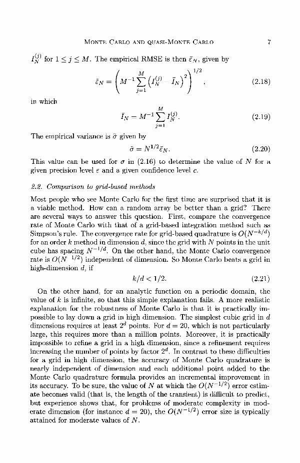
To demonstrate how quasi-random sequences depend on dimension, we willpresent results from two computational tests. The first is a computation ofI? discrepancy for a quasi-random sequence. The second is an examinationof the one- and two-dimensional projections of quasi-random sequences.

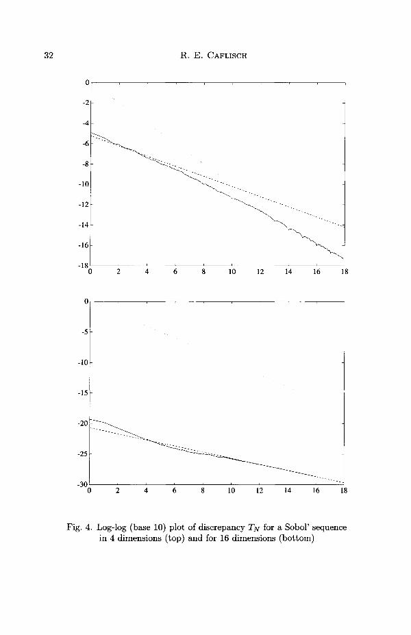
The L2 discrepancy T/v can be computed directly (Morokoff and Caflisch1994) by an explicit formula. Figure 4 shows computation of T/v for a Sobol'sequence for dimension 4 and 16. In addition to Tjv, each graph shows aplot of TV"1/2 with a constant coming from the expected discrepancy of arandom sequence. Each graph also shows a plot of N^1 (with a constant of

32 R. E. CAFLISCH

10 12 14 16

8 10 12 14 16 18

Fig. 4. Log-log (base 10) plot of discrepancy T/v for a Sobol' sequencein 4 dimensions (top) and for 16 dimensions (bottom)


no significance). Since the plots are on a log-log scale, these reference curvesare lines of slope — 1/2 and — 1.

The figure for small dimension (4) and for large N, shows that T/v ~O(N~1). We have not tried to match the logN terms, since we do not seemto be able to detect them reliably. On the other hand, the graph for largedimension (16), shows that for moderate sized N, TJV ~ O(N~1^2), with aconstant that agrees with the discrepancy of a random sequence. Eventually,as N gets very large, T/v must be nearly of size O(N~1). The agreementbetween discrepancy of quasi-random and random sequences for large d andmoderate N has not been explained.

Next we consider one- and two-dimensional projections of a quasi-randomsequence. Many, but not all, quasi-random sequences have the followingspecial property. All one-dimensional projections of the sequence {i.e., allsingle components) are equally well distributed. The Sobol' sequence, forexample, has this property. This implies that any function / that consists ofa sum of one-dimensional functions will be well integrated by quasi-MonteCarlo, in other words, functions of the form

/n(*n). (5.27)n=l

In particular, quasi-Monte Carlo performs very well for linear functions

d

f(x) « âjXj. (5.28)i= l

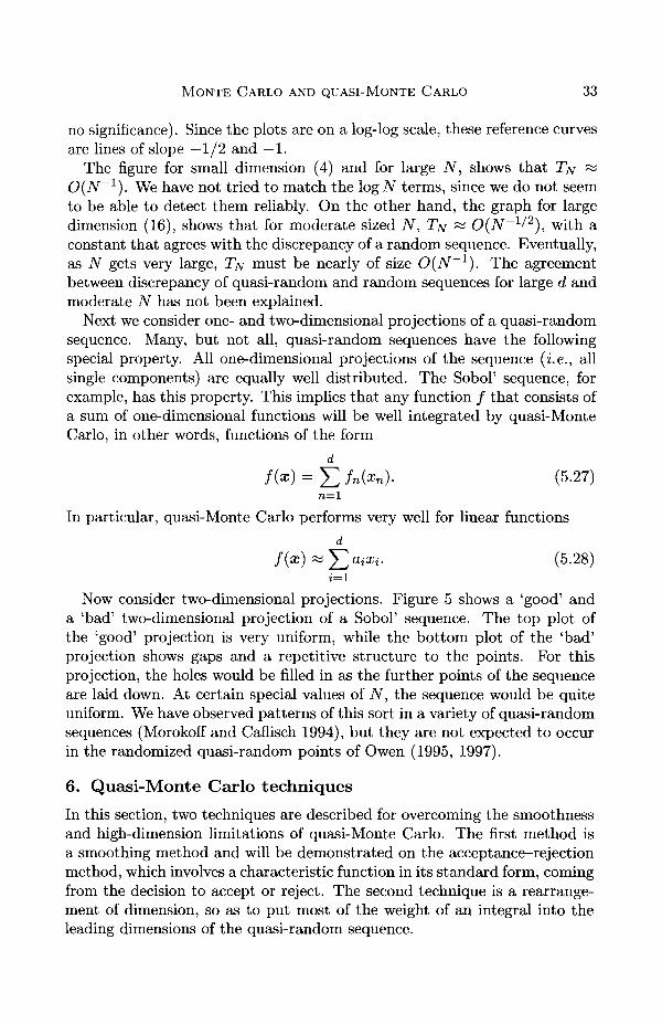
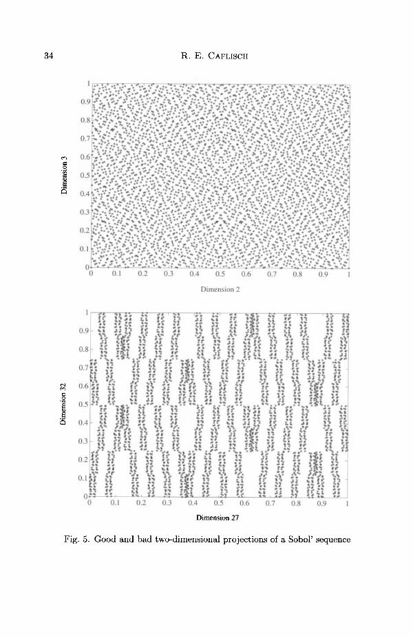
Now consider two-dimensional projections. Figure 5 shows a 'good' anda 'bad' two-dimensional projection of a Sobol' sequence. The top plot ofthe 'good' projection is very uniform, while the bottom plot of the 'bad'projection shows gaps and a repetitive structure to the points. For thisprojection, the holes would be filled in as the further points of the sequenceare laid down. At certain special values of N, the sequence would be quiteuniform. We have observed patterns of this sort in a variety of quasi-randomsequences (Morokoff and Caflisch 1994), but they are not expected to occurin the randomized quasi-random points of Owen (1995, 1997).

6. Quasi-Monte Carlo techniques

In this section, two techniques are described for overcoming the smoothnessand high-dimension limitations of quasi-Monte Carlo. The first method isa smoothing method and will be demonstrated on the acceptance-rejectionmethod, which involves a characteristic function in its standard form, comingfrom the decision to accept or reject. The second technique is a rearrange-ment of dimension, so as to put most of the weight of an integral into theleading dimensions of the quasi-random sequence.

34 R. E. CAFLISCH

S

o.i 0.2 0.3 0.4 0.5 0.6 0.7 0.8 0.9

Dimension 2

if niff iiiii

it It 1 !i p lil i

0.7 0.8 0.9

Dimension 27

Fig. 5. Good and bad two-dimensional projections of a Sobol' sequence


6.1. Smoothing

The effectiveness of quasi-Monte Carlo is often lost on problems involvingdiscontinuities, such as decisions in the acceptance-rejection method. Oneway to overcome this difficulty is to smooth out the integrand without chan-ging the value of the integral. Here we describe a smoothed version ofthe acceptance-rejection method and compare it with standard acceptance-rejection, when used with a quasi-random sequence.

Standard acceptance—rejection can be expressed in an integration problemin the following way. Consider the integral of a function / multiplying afunction p on the unit interval, with 0 < p(x) < 1. Rewrite the integral as

f1 f1 f1

/ f(x)p(x)dx = / f(x)X(y <p(x))dydx. (6.1)Jo Jo Jo

The acceptance-rejection method is a slight modification of the usual MonteCarlo formula for this integral, that is,

• sample (x, y) uniformly• weight w = x{y < p(%)) — 1 (accept), if y < p(x)• weight w = x(y < P(x)) — 0 (reject), if y > p{x)• repeat until number of accepted points is N.

The Monte Carlo quadrature formula is then

M

Wif(xi), (6.2)

in whichM

(6.3)

The smoothed acceptance-rejection method (Spanier and Maize 1994,Moskowitz and Caflisch 1996) is formulated by replacing the discontinuousfunction x(y < p(x)) by a smooth function q(x,y) satisfying

/ q(x,y)dy=p(x). (6.4)Jo

For example, one choice of q is a piecewise linear function:

{ 1 if y < p(x) - e,

0 if y > p(x) + e, (6.5)linear p(x) — e < y < p(x) + e.

The integral can then be rewritten as/ f(x)p(x)dx= f f f(x)q(x,y)dydx, (6.6)Jo Jo Jo

36 R. E. CAFLISCH

10'

10"

CO

I2

LLJ

-10'

10

10 -

10""

KEY (convergence rate)

Raw Monte Carlo: (-.52)Weighted unit, sampling: (-.49)Rejection method: . . . (-.50)Smooth rej., delta = .2: _ . _ (-.51)

10'N

10° 10°

10"

10"

IUJ

10"'-

10-


Raw Monte Carlo: (-.96)Weighted unif. sampling: (-96)Rejection method: . . . (-.66)Smooth rej., delta = .2: _ . _ (-.88)

10" 10'N

10° 10"

Fig. 6. Smoothed acceptance-rejection for Monte Carlo (top)and quasi-Monte Carlo (bottom)


and the sampling procedure is the following:

• sample (x, y) uniformly• set the weight w = q(x, y)• repeat until

M

,yi)~N. (6.7)

The quadrature formula, using smoothed acceptance-rejection, is then

M

JN = N-1J2<l(xi,yi)f(xi), (6.8)

in whichM

q{xi,yi)~N. (6.9)

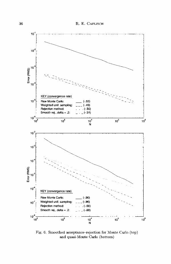
Figure 6 shows the results of standard and smoothed acceptance—rejectionfor Monte Carlo using both a pseudo-random sequence and a quasi-randomsequence. The integral evaluated here (Moskowitz and Caflisch 1996) hasthe form

x)ax, (6.10)JI<

in which I7 = [0,1]7 and

p(x) = exp | - ^sin2 (^|îj + sin2 \^x2j + sin2 ( ^ a -ij) J) J-,

/(a;) = e arcsm sin(l)+ — . (6.11)

The integral / is evaluated in several ways. First, by 'raw Monte Carlo',by which we mean evaluation of the product f(x)p(x) at points from auniformly distributed sequence. Second, points are sampled from the (un-normalized) density function p using acceptance-rejection, then / is eval-uated at these points. Third, standard acceptance-rejection is replacedby smoothed acceptance-rejection. Finally, all three of these methods areperformed both with pseudo-random and quasi-random points. These nu-merical results show the following.

• Importance sampling, using acceptance-rejection, reduces variance andleads to smaller errors for both Monte Carlo and quasi-Monte Carlo.

• For Monte Carlo, smoothing has little effect on errors, since it does notchange the variance.

• Without importance sampling, the quasi-Monte Carlo method con-verges at a rapid rate, but with a constant that is larger than for themethod with importance sampling.

38 R. E. CAFLISCH

• For quasi-Monte Carlo, the error for unsmoothed acceptance-rejectiondecreases at a slower rate, because of discontinuities involved in theacceptance-rejection decision.

• For quasi-Monte Carlo, the rapid convergence rate is regained usingsmoothing.

Although smoothed acceptance—rejection regains much of the effective-ness of quasi-Monte Carlo, it entails a loss of efficiency. Since fractionalweights are involved, more accepted samples are required to get total weightN. Moreover, we do not have an effective quasi-Monte Carlo method forthe Metropolis algorithm (Kalos and Whitlock 1986), which is a stochasticprocess involving acceptance-rejection.

6.2. Dimension reduction: Brownian bridge method

For problems in a dimension of moderate size, quasi-Monte Carlo providesa significant speed-up over standard Monte Carlo. Many of the most im-portant applications of Monte Carlo, however, involve integrals of a veryhigh dimension. One class of examples comprises path integrals involvingBrownian motion b(t). A typical example is a Feynman-Kac integral (Kar-atzas and Shreve 1991) of the form

I = E j f(b(t))expi f \{b{s),s)ds\ dt (6.12)

In order to evaluate this expectation by Monte Carlo, we need to discretizethe time in the Brownian motion to obtain a random walk with M steps.Then the integral becomes an integral over the M steps of a random walk,each of which is distributed by a normal distribution. An accurate rep-resentation of the integral requires a large number M of time-steps, whichresults in an integral of large-dimension M. Because of the high dimension,we find that quasi-Monte Carlo loses much of its effectiveness on such aproblem. The main point of this section is to show how a rearrangementof the dimensions can regain the effectiveness of quasi-Monte Carlo for thisproblem.

The standard discretization of a random walk is to represent the positionb(t + At) in terms of the previous position b(t) by the formula

b(t + At) = b(t) + VAt v, (6.13)

in which v is an N(0,1) random variable. Using a sequence of independentsamples of is, we can generate the random walk sequentially by

j/o = 0, y i = b(At), y 2 = b(2At),.... (6.14)

This representation leads to the M-dimensional integral discussed above.


16

14

12

10

• 8

6

4-

2-

-3 -2 -1

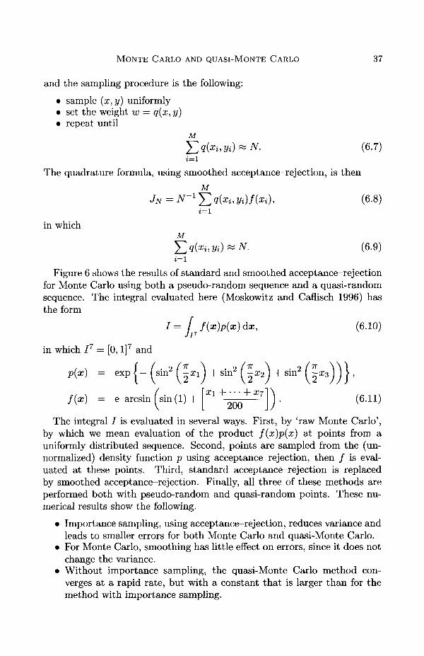
Fig. 7. Standard discretization of random walk

The effectiveness of quasi-Monte Carlo will be regained using an alternat-ive representation of the random walk, the Brownian bridge discretization,which was first introduced as a quasi-Monte Carlo technique by Moskowitzand Caflisch (1996). This representation relies on the following Brownianbridge formula (Karatzas and Shreve 1991) for b(t + At\), given b(t) andb(T = t + Ah + At2):

b(t + Ah) = ab(t) + (1 - a)b(T) + cu, (6.15)

in which

a = At2/(Ah + At2) (6.16)

Using this representation, the random walk can be generated by successivesubdivision. Suppose for simplicity that M is a power of 2. Then generatethe random walk in the following order:

V0 = 0 , D M , V M / 2 , V M / 4 , V 3 M / 4 , •••• (6-17)

The standard discretization and Brownian bridge discretization are repres-ented schematically in Figures 7 and 8.

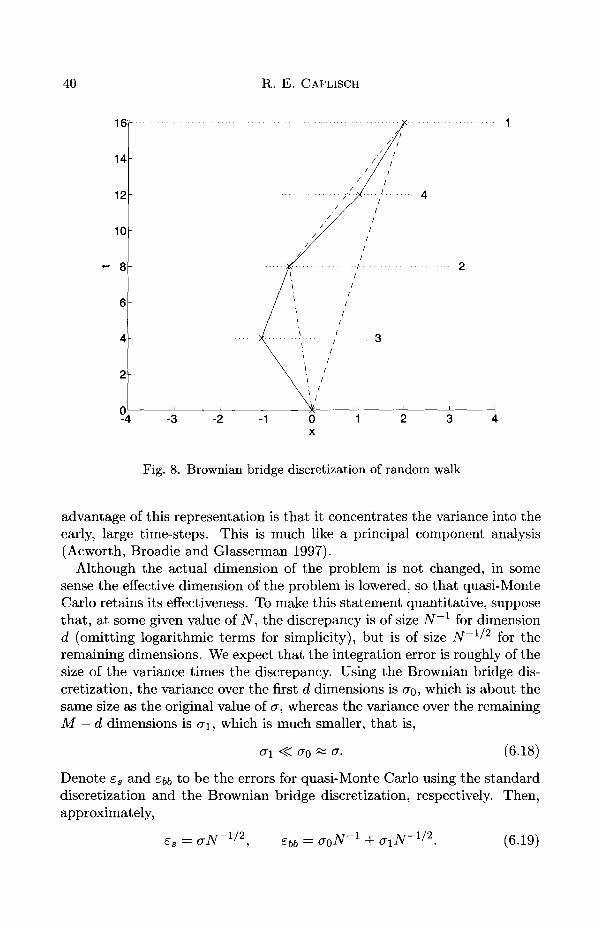
The significance of this representation is that it first chooses the largetime-steps over which the changes in b(t) are large. Then it fills in the smalltime-steps in between, in which the changes in b(t) are quite small. The

40 R. E. CAFLISCH

16-

14

12

10

8-

6-

4

-3 -2 -1

Fig. 8. Brownian bridge discretization of random walk

advantage of this representation is that it concentrates the variance into theearly, large time-steps. This is much like a principal component analysis(Acworth, Broadie and Glasserman 1997).

Although the actual dimension of the problem is not changed, in somesense the effective dimension of the problem is lowered, so that quasi-MonteCarlo retains its effectiveness. To make this statement quantitative, supposethat, at some given value of N, the discrepancy is of size N^1 for dimensiond (omitting logarithmic terms for simplicity), but is of size N~ll2 for theremaining dimensions. We expect that the integration error is roughly of thesize of the variance times the discrepancy. Using the Brownian bridge dis-cretization, the variance over the first d dimensions is CTO, which is about thesame size as the original value of a, whereas the variance over the remainingM — d dimensions is ai, which is much smaller, that is,

(j\ <?C fo ~ &• (6.18)

Denote es and Ebb to be the errors for quasi-Monte Carlo using the standarddiscretization and the Brownian bridge discretization, respectively. Then,approximately,

es = ebb = (6.19)


10'

10"

10 -

ILJJ

10 -

1 0 -

10"'


Pseudo-random, std discr.:

Halton seq., std discr.:

Pseudo-random, alt. discr.:

Halton seq., alt. discr.:

-

(-•51)

_ • _ (-.77) ^

. . .(-.so) ;

(-.95)

, t ,

10' 10°

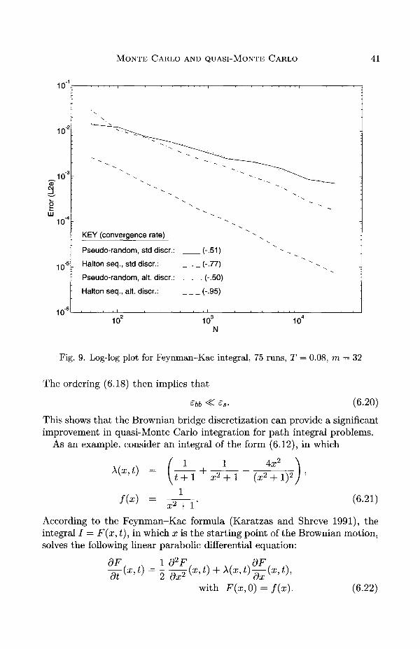
Fig. 9. Log-log plot for Feynman-Kac integral, 75 runs, T = 0.08, m = 32

The ordering (6.18) then implies that

£bb < (6.20)

This shows that the Brownian bridge discretization can provide a significantimprovement in quasi-Monte Carlo integration for path integral problems.

As an example, consider an integral of the form (6.12), in which

X(x,t) = 1 1—r + r~

4x2

(6.21)

According to the Feynman-Kac formula (Karatzas and Shreve 1991), theintegral / = F(x, t), in which x is the starting point of the Brownian motion,solves the following linear parabolic differential equation:

^ t\ = I S^L(X t) + X(x t) — (x t)dx

with F(x,0) = f(x). (6.22)

42 R. E. CAFLISCH

The exact solution is F(x,t) = (t + l)(x2 + I ) " 1 .Computational results for this problem of Moskowitz and Caflisch (1996)

are presented in Figure 9, at time T = 0.08 with M = 32. The results showthe following.

• For Monte Carlo using pseudo-random numbers, the error is the samefor the standard and Brownian bridge discretizations. This is becausethe variance of the two is the same.

• For quasi-Monte Carlo with the standard discretization, the error isonly a little less than for standard Monte Carlo; i.e., the effectivenessof quasi-Monte Carlo has been lost for this high-dimension (M = 32).

• With the Brownian bridge discretization, the error for quasi-MonteCarlo is substantially reduced, in terms of both the rate of convergenceand the constant; i.e., the effectiveness of quasi-Monte Carlo has beenregained.

It is necessary to use the transformation method (Section 3.3) rather thanthe Box-Muller method (Section 3.4), since the latter method has largegradients (Morokoff and Caflisch 1993). Similar results have been obtainedon problems from computational finance by Caflisch, Morokoff and Owen(19976).

7. Monte Carlo methods for rarefied gas dynamics

Computations for rarefied gas dynamics, as occur in the outer parts of theatmosphere, are difficult since the gas is represented by a distribution func-tion over space, time and molecular velocity. For general problems, the onlyeffective method has been a Monte Carlo method, as described below. Onereason for including this application of Monte Carlo in this survey is thatformulation of an effective Monte Carlo method in the fluid dynamic limitis an open problem.

7.1. The Boltzmann equation

The kinetic theory of gases describes the behaviour of a gas in which thedensity is not too large, so that the only interactions between gas particlesare binary collisions. The resulting nonlinear Boltzmann equation,

for the molecular distribution function F(x,£,t), is a basic equation ofnonequilibrium statistical mechanics (Cercignani 1988, Chapman and Cowl-ing 1970). The collision operator is

Q(F,F)(C = | ( F « i ) F « ' ) - F(^)F^))B(LJ, \d ~ *|)da;d4i, (7.2)


in which £, £j represent velocities before a collision, £', £[ represent velocitiesafter a collision, and the collision parameters are represented by w € 5 2 ,where S2 is the unit sphere in M3. The parameter e is a measure of the 'meanfree time', which is defined as the characteristic time between collisions of aparticle.

For a molecular distribution F, the macroscopic (or fluid dynamic) vari-ables are the density p, velocity u and temperature T defined by

P =

u =

T = (3P)-1 J\£-u\2Fdt (7.3)

The importance of these moments of F is that they correspond to conservedquantities, namely, mass, momentum and energy, for the collisional process,which is expressed as follows:

/Q(F,F)d£ = 0,

£Q(F,F)d$ = 0,

2 = 0. (7.4)

These also provide the degrees of freedom for the equilibrium case, the Max-wellian distributions

M(£, p, u, T) = p(27rr)-3/2 exp ( - | £ - u\2/2T) . (7.5)

In the limit e —> 0, the solution F of ( 7.1) is given by the Hilbert (orChapman-Enskog) expansion, in which the leading term is a Maxwelliandistribution of the form (7.5), in which p, u, T satisfy the compressibleEuler (or Navier-Stokes) equations of fluid dynamics (Chapman and Cowl-ing 1970). The Euler equations are

pt + V • (up) = 0,(pu)t + V • (uup) + V(pT) = 0,

This expansion is not valid in layers around shocks, boundaries and non-equilibrium initial data, where special boundary, shock or initial layer ex-pansions can be constructed (Caflisch 1983). By varying this limit, takingthe velocity u to be size e as well, the compressible equations are replaced

44 R. E. CAFLISCH

by the incompressible fluid equations (Bardos, Golse and Levermore 1991,1993, De Masi, Esposito and Lebowitz 1989).

7.2. Particle methods

In particle methods for transport theory, the distribution F(x., £, t) is rep-resented as the sum

N

FN(X,£,t) = J26(Z- U*)W* - *»(*)), (7-7)7 1 = 1

and the positions xn(£) and velocities £n(t) are evolved in time to simulatethe effects of convection and collisions. The most common particle methodsuse random collisions between a reasonable number of particles (e.g., 103-106) to simulate the dynamics of many particles (e.g., 1023).

In the direct simulation Monte Carlo (DSMC) method pioneered by Bird(1976, 1978), the numerical method is designed to simulate the physicalprocesses as closely as possible. This makes it easy to understand and toinsert new physics; it is also numerically robust. First, space and timeare discretized into spatial cells of size Ax3 and time-steps of duration At.In each time-step the evolution is divided into two steps: transport andcollisions. For the transport step each particle is moved from position xn(£)to xn(t + At) = xn(t) + At£„(*).

In the collision step, random collisions are performed between particleswithin each spatial bin. In each collision, particles £n and £m are chosenrandomly from the full set of particles in a bin, with probability pmn givenby

_ ff([srn £nl) in o\"52l<i<j<N0 S(\£i — £j\)

in which No is the number of particles in the spatial bin, and

,\£m-U)&» (7-9)s2

is the total collision rate between particles of velocity £j and £,•. As written,this choice requires O(N2) operations to evaluate the sum in the denom-inator in (7.8). By a standard acceptance—rejection scheme, however, eachchoice can be made in 0(1) steps, so that the total method requires onlyO(N) steps.

Next the collision parameters u> are randomly chosen from a uniform dis-tribution on S2. The outcome of the collision is two new velocities £'n and£'m which replace the old velocities £n and £m.

The number of collisions performed in each time-step has been determinedby several methods. In the original 'time-counter' (TC) method, a collision


time Atc is determined. It is equal to one over the frequency for that collisiontype, that is,

Atc = 2(nN0S^m-U))~1, (7.10)

in which n is the number density of particles. This is added to the time-counter tc = J2 Atc. In the time interval of length At beginning at t, colli-sions are continued until tc exceeds the final time, that is, until tc > t + At.For N particles this method has operation count O(N).

The unlikely possibility of choosing a collision with very small frequencycan result in a large collisional time-step that may cause relatively largeerrors. To remove such errors, Bird (1976) has developed a 'no time-counter'(NTC) method. This method uses a maximum collision probability 5m a x .The number of collisions to be performed in time-step dt is chosen as if thecollision frequency were exactly 5m a x for all collision pairs. For each selectionof a collision pair, the collision between £m and £„ is then performed withprobability S(\£m — £n\)/Smax, as in an acceptance-rejection scheme. TheDSMC method with the time-counter or no-time-counter algorithm has beenenormously successful. A rigorous convergence result for DSMC was provedby Wagner (1992).

Several related methods have been developed by other researchers, in-cluding Koura (1986), Nanbu (1986), and Goldstein, Sturtevant and Broad-well (1988). Additional modifications of Nanbu's method, including use ofquasi-random sequences, have been developed by Babovsky, Gropengiesser,Neunzert, Struckmeier and Wiesen (1990).

7.3. Methods with the correct diffusion limit

One of the most difficult problems of transport theory is that there may bewide variation of mean free paths within a single problem. In regions wherethe mean free path is large, there are few collisions, so that large numericaltime-steps may be taken, whereas in regions where the mean free path issmall, the time- and space-steps must be small. Thus the highly collisionalregions determine the numerical time-step, which may make computationsimpractically slow. On the other hand, much of the extra effort in thecollisional regions seems wasted, since in those regions the gas will be nearlyin fluid dynamic equilibrium, so that a fluid dynamic description (7.6) shouldbe valid.

A partial remedy to this problem is to use a numerical method that con-verts to a numerical method for the correct fluid equations in regions wherethe mean free time is small. This allows large, fluid dynamic time-steps inthe collisional region and large collisional time-steps in the large mean freetime region.

Consider a discretization of the Boltzmann equation (7.1) with discretespace and time scales Ax and At. If Ax, At are much smaller than e, then

46 R. E. CAFLISCH

the Boltzmann solution is well resolved. On the other hand, in regions ofsmall mean free path, we want to let the discretization scale be much largerthan the collision scale e. So we consider the limit in which the numericalparameters Ax, At are held fixed, while e —> 0. We say that the discretizedequation has the correct diffusion limit, if in this limit the solution of thediscrete equations for (7.1) goes to the solution for a discretization of thefluid equation (7.6).

In the context of linear neutron transport, Larsen and co-workers (Larsen,Morel and Miller 1987, Borgers, Larsen and Adams 1992) have investigatedthe diffusion limit for a variety of difference schemes and have found thatmany of them have the correct diffusion limit only in special regimes. Theyhave constructed some alternative methods that always have the correctdiffusion limit. Jin and Levermore (1993) have applied a similar procedureto an interface problem to get a constraint on the quadrature set for thediscretization of a scattering integral. Another class of methods that usesinformation from the diffusion limit to improve a numerical transport meth-ods is the family of 'diffusion synthetic acceleration methods' (Larsen 1984).For the Broadwell model of the Boltzmann equation, finite difference numer-ical methods with the correct diffusion limit have been developed (Caflisch,Jin and Russo 1997a, Jin, Pareschi and Toscani 1998). These use implicitdifferencing for the collision step, because it is a stiff problem with rate e"1.

For the nonlinear Boltzmann equation, on the other hand, Monte Carlomethods are the most practical because of the large number of degrees offreedom. Application of the methods would require some kind of implicitstep to handle the collisions, but no such method has been formulated so far.We believe that a method that uses fluid dynamic information to improvethe collisional step for rarefied gas dynamic computations would have greatimpact. Some important partial steps in this direction have been taken(Gabetta, Pareschi and Toscani 1997), but they have not yet been extendedto particle methods such as DSMC.

REFERENCESP. Acworth, M. Broadie and P. Glasserman (1997), A comparison of some Monte

Carlo and quasi Monte Carlo techniques for option pricing, in Monte Carlo andQuasi-Monte Carlo Methods 1996 (G. Larcher, H. Niederreiter, P. Hellekalekand P. Zinterhof, eds), Springer.

H. Babovsky, F. Gropengiesser, H. Neunzert, J. Struckmeier and J. Wiesen (1990),'Application of well-distributed sequences to the numerical simulation of theBoltzmann equation', J. Comput. Appl. Math. 31, 15-22.

C. Bardos, F. Golse and C. D. Levermore (1991), 'Fluid dynamic limits of kineticequations: I. Formal derivations', J. Statist. Phys. 63, 323-344.


C. Bardos, F. Golse and C. D. Levermore (1993), 'Fluid dynamic limits of kineticequations: II. Convergence proofs for the Boltzmann equation', Comm. PureAppl. Math. 46, 667-753.

G. A. Bird (1976), Molecular Gas Dynamics, Oxford University Press.G. A. Bird (1978), 'Monte Carlo simulation of gas flows', Ann. Rev. Fluid Mech.

10, 11-31.C. Borgers, E. W. Larsen and M. L. Adams (1992), 'The asymptotic diffusion limit

of a linear discontinuous discretization of a two-dimensional linear transportequation', J. Comput. Phys. 98, 285-300.

P. Bratley, B. L. Fox and H. Niederreiter (1994), 'Algorithm 738 - Programs togenerate Niederreiter's discrepancy sequences', A CM Trans. Math. Software20, 494-495.

R. E. Caflisch (1983), Fluid dynamics and the Boltzmann equation, in Nonequi-librium Phenomena I: The Boltzmann equation (E. W. Montroll and J. L.Lebowitz, eds), Vol. 10 of Studies in Statistical Mechanics, North Holland,pp. 193-223.

R. E. Caflisch, S. Jin and G. Russo (1997a), 'Uniformly accurate schemes for hy-perbolic systems with relaxation', SIAM J. Numer. Anal. 34, 246-281.

R. E. Caflisch, W. Morokoff and A. B. Owen (19976), 'Valuation of mortgage-backedsecurities using Brownian bridges to reduce effective dimension', J. Comput.Finance 1, 27-46.

C. Cercignani (1988), The Boltzmann Equation and its Applications, Springer.S. Chapman and T. G. Cowling (1970), The Mathematical Theory of Non-Uniform

Gases, Cambridge University Press.A. De Masi, R. Esposito and J. L. Lebowitz (1989), 'Incompressible Navier-

Stokes and Euler limits of the Boltzmann equation', Comm. Pure Appl. Math.42, 1189-1214.

H. Faure (1982), 'Discrepance de suites associees a un systeme de numeration (endimension s)\ Ada Arithmetica 41, 337-351.

W. Feller (1971), An Introduction to Probability Theory and its Applications: Vol.I, Wiley.

E. Gabetta, L. Pareschi and G. Toscani (1997), 'Relaxation schemes for nonlinearkinetic equations', SIAM J. Numer. Anal. 34, 2168-2194.

D. Goldstein, B. Sturtevant and J. E. Broadwell (1988), Investigations of the mo-tion of discrete-velocity gases, in Rarefied Gas Dynamics: Theoretical andComputational Techniques (E. P. Muntz, D. P. Weaver and D. H. Campbell,eds), Vol. 118 of Progress in Aeronautics and Astronautics, Proceedings of the16th International Symposium on Rarefied Gas Dynamics, pp. 100-117.

J. H. Halton (1960), 'On the efficiency of certain quasi-random sequences of pointsin evaluating multi-dimensional integrals', Numer. Math. 2, 84-90.

J. M. Hammersley and D. C. Handscomb (1965), Monte Carlo Methods, Wiley,New York.

C. Haselgrove (1961), 'A method for numerical integration', Math. Comput.15, 323-337.

F. J. Hickernell (1996), 'The mean square discrepancy of randomized nets', ACMTrans. Model. Comput. Simul. 6, 274-296.

48 R. E. CAFLISCH

F. J. Hickernell (1998), 'A generalized discrepancy and quadrature error bound',Math. Comput. 67, 299-322.

R. V. Hogg and A. T. Craig (1995), Introduction to Mathematical Statistics, Pren-tice Hall.

L. K. Hua and Y. Wang (1981), Applications of Number Theory to NumericalAnalysis, Springer, Berlin/New York.

S. Jin and C. D. Levermore (1993), 'Fully-discrete numerical transfer in diffusiveregimes', Transp. Theory Statist. Phys. 22, 739-791.

S. Jin, L. Pareschi and G. Toscani (1998), 'Diffusive relaxation schemes for discrete-velocity kinetic equations'. Preprint.

M. H. Kalos and P. A. Whitlock (1986), Monte Carlo Methods, Vol. I: Basics,Wiley, New York.

I. Karatzas and S. E. Shreve (1991), Brownian Motion and Stochastic Calculus,Springer, New York.

W. J. Kennedy and J. E. Gentle (1980), Statistical Computing, Dekker, New York.K. Koura (1986), 'Null-collision technique in the direct-simulation Monte Carlo

method', Phys. Fluids 29, 3509-3511.L. Kuipers and H. Niederreiter (1974), Uniform Distribution of Sequences, Wiley,

New York.E. W. Larsen (1984), 'Diffusion-synthetic acceleration methods for discrete-

ordinates problems', Transp. Theory Statist. Phys. 13, 107-126.E. W. Larsen, J. E. Morel and W. F. Miller (1987), 'Asymptotic solutions of nu-

merical transport problems in optically thick, diffusive regimes', J. Comput.Phys. 69, 283-324.

G. Lepage (1978), 'A new algorithm for adaptive multidimensional integration',J. Comput. Phys. 27, 192-203.

G. Marsaglia (1991), 'Normal (Gaussian) random variables for supercomputers',J. Supercomputing 5, 49-55.

W. Morokoff and R. E. Caflisch (1993), 'A quasi-Monte Carlo approach to particlesimulation of the heat equation', SIAM J. Numer. Anal. 30, 1558-1573.

W. Morokoff and R. E. Caflisch (1994), 'Quasi-random sequences and their discrep-ancies', SIAM J. Sci. Statist. Comput. 15, 1251-1279.

W. Morokoff and R. E. Caflisch (1995), 'Quasi-Monte Carlo integration', J. Comput.Phys. 122, 218-230.

B. Moskowitz and R. E. Caflisch (1996), 'Smoothness and dimension reduction inquasi-Monte Carlo methods', J. Math. Comput. Modeling 23, 37-54.

K. Nanbu (1986), Theoretical basis of the direct simulation Monte Carlo method, inProceedings of the 15th International Symposium on Rarefied Gas Dynamics(V. Bom and C. Cercignani, eds), Vol. I, pp. 369-383.

H. Niederreiter (1992), Random Number Generation and Quasi-Monte Carlo Meth-ods, SIAM, Philadelphia, PA.

A. B. Owen (1995), Randomly permuted (t, m, s)-nets and (t, s)-sequences, inMonte Carlo and Quasi-Monte Carlo Methods in Scientific Computing(H. Niederreiter and P. J.-S. Shiue, eds), Springer, New York, pp. 299-317.

A. B. Owen (1997), 'Monte Carlo variance of scrambled net quadrature', SIAMJ. Numer. Anal. 34, 1884-1910.


A. B. Owen (1998), 'Scrambled net variance for integrals of smooth functions', Ann.Statist. In press.

W. H. Press and S. A. Teukolsky (1992), 'Portable random number generators',Corn-put. Phys. 6, 522-524.

W. H. Press, S. A. Teukolsky, W. T. Vettering and B. P. Flannery (1992), NumericalRecipes in C: The AH of Scientific Computing, 2nd edn, Cambridge UniversityPress.

D. I. Pullin (1979), 'Generation of normal variates with given sample and meanvariance', J. Statist. Comput. Simul. 9, 303-309.

I. M. Sobol' (1967), 'The distribution of points in a cube and the accurate evaluationof integrals', Zh. Vychisl. Mat. Mat. Fiz. 7, 784-802. In Russian.

I. M. Sobol' (1976), 'Uniformly distributed sequences with additional uniformityproperty', USSR Comput. Math. Math. Phys. 16, 1332-1337.

J. Spanier and E. H. Maize (1994), 'Quasi-random methods for estimating integralsusing relatively small samples', SIAM Rev. 36, 18-44.

W. Wagner (1992), 'A convergence proof for Bird's Direct Simulation Monte Carlomethod for the Boltzmann equation', J. Statist. Phys. 66, 1011-1044.

H. Wozniakowski (1991), 'Average case complexity of multivariate integration',Bull. Amer. Math. Soc. 24, 185-194.

C. P. Xing and H. Niederreiter (1995), 'A construction of low-discrepancy sequencesusing global function fields', Ada Arithmetica 73, 87-102.

S. K. Zaremba (1968), 'The mathematical basis of Monte Carlo and quasi-MonteCarlo methods', SIAM Rev. 10, 303-314.

Documents

Monte Carlo and quasi-Monte Carlo methods - PKUdsec.pku.edu.cn/~tieli/notes/numer_anal/MCQMC_Caflisch.pdf · MONTE CARLO AND QUASI-MONTE CARLO 3 quasi-random points converges more