Embed Size (px)
Citation preview
Optim Lett (2015) 9:949–960DOI 10.1007/s11590-014-0837-4
ORIGINAL PAPER
A parallel branch and bound algorithmfor the maximum labelled clique problem
Ciaran McCreesh · Patrick Prosser
Received: 18 August 2014 / Accepted: 18 November 2014 / Published online: 10 December 2014© The Author(s) 2014. This article is published with open access at Springerlink.com
Abstract The maximum labelled clique problem is a variant of the maximum cliqueproblemwhere edges in the graph are given labels, and we are not allowed to use morethan a certain number of distinct labels in a solution. We introduce a new branch-and-bound algorithm for the problem, and explain how it may be parallelised. We evaluatean implementation on a set of benchmark instances, and show that it is consistentlyfaster than previously published results, sometimes by four or five orders ofmagnitude.
Keywords Maximum labelled clique · Parallel branch and bound ·Combinatorial optimisation · Computational experiments
1 Introduction
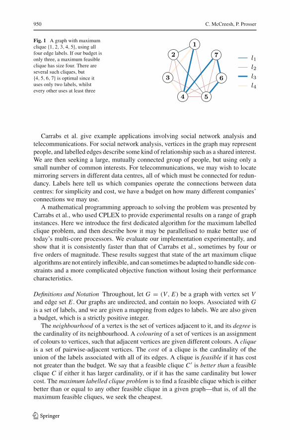
A clique in a graph is a set of vertices, where every vertex in this set is adjacent toevery other in the set. Finding the size of a maximum clique in a given graph is oneof the fundamental NP-hard problems. Carrabs et al. [1] introduced a variant calledthe maximum labelled clique problem. In this variant, each edge in the graph has alabel, and we are given a budget b: we seek to find as large a clique as possible, butthe edges in our selected clique may not use more than b different labels in total. Inthe case that there is more than one such maximum, we must find the one using fewestdifferent labels. We illustrate these concepts in Fig. 1, using an example graph due toCarrabs et al.; our four labels are shown using different styled edges.
C. McCreesh (B) · P. ProsserUniversity of Glasgow, Glasgow, Scotlande-mail: [email protected]
P. Prossere-mail: [email protected]
123
950 C. McCreesh, P. Prosser
Fig. 1 A graph with maximumclique {1, 2, 3, 4, 5}, using allfour edge labels. If our budget isonly three, a maximum feasibleclique has size four. There areseveral such cliques, but{4, 5, 6, 7} is optimal since ituses only two labels, whilstevery other uses at least three
1
2
3
4 5
6
7 l1
l2
l3
l4
Carrabs et al. give example applications involving social network analysis andtelecommunications. For social network analysis, vertices in the graph may representpeople, and labelled edges describe some kind of relationship such as a shared interest.We are then seeking a large, mutually connected group of people, but using only asmall number of common interests. For telecommunications, we may wish to locatemirroring servers in different data centres, all of which must be connected for redun-dancy. Labels here tell us which companies operate the connections between datacentres: for simplicity and cost, we have a budget on how many different companies’connections we may use.
A mathematical programming approach to solving the problem was presented byCarrabs et al., who used CPLEX to provide experimental results on a range of graphinstances. Here we introduce the first dedicated algorithm for the maximum labelledclique problem, and then describe how it may be parallelised to make better use oftoday’s multi-core processors. We evaluate our implementation experimentally, andshow that it is consistently faster than that of Carrabs et al., sometimes by four orfive orders of magnitude. These results suggest that state of the art maximum cliquealgorithms are not entirely inflexible, and can sometimes be adapted to handle side con-straints and a more complicated objective function without losing their performancecharacteristics.
Definitions and Notation Throughout, let G = (V, E) be a graph with vertex set Vand edge set E . Our graphs are undirected, and contain no loops. Associated with Gis a set of labels, and we are given a mapping from edges to labels. We are also givena budget, which is a strictly positive integer.
The neighbourhood of a vertex is the set of vertices adjacent to it, and its degree isthe cardinality of its neighbourhood. A colouring of a set of vertices is an assignmentof colours to vertices, such that adjacent vertices are given different colours. A cliqueis a set of pairwise-adjacent vertices. The cost of a clique is the cardinality of theunion of the labels associated with all of its edges. A clique is feasible if it has costnot greater than the budget. We say that a feasible clique C ′ is better than a feasibleclique C if either it has larger cardinality, or if it has the same cardinality but lowercost. The maximum labelled clique problem is to find a feasible clique which is eitherbetter than or equal to any other feasible clique in a given graph—that is, of all themaximum feasible cliques, we seek the cheapest.
123

The maximum labelled clique problem 951
The hardness of the maximum clique problem immediately implies that the maxi-mum labelled clique problem is also NP-hard. Carrabs et al. showed that the problemremains hard even for complete graphs, where the maximum clique problem is trivial.
2 A branch and bound algorithm
In Algorithm 1 we present the first dedicated algorithm for the maximum labelledclique problem. This is a branch and bound algorithm, using a greedy colouring forthe bound. We start by discussing how the algorithm finds cliques, and then explainhow labels and budgets are checked.
Algorithm 1: An algorithm for the maximum labelled clique problem.1 maximumLabelledClique : : (Graph G, Int budget) → Vertex Set2 begin3 permute G so that vertices are in non-increasing degree order4 global (C�, L�) ← (∅, ∅)5 expand(true, ∅, every vertex of G, ∅)6 expand(false, ∅, every vertex of G, ∅)7 return C� (unpermuted)
8 expand : : (Boolean first, Vertex Set C , Vertex Set P, Label Set L)9 begin
10 (order, bounds) ← colourOrder(P)11 for i ← |P| downto 1 do12 if |C | + bounds[i] < |C�| or (first and |C | + bounds[i] = |C�|) then13 return
14 v ← order[i]15 add v to C16 L ′ ← L ∪ the labels of edges between v and any vertex in C17 if |L ′| ≤ (budget if first, otherwise |L�| − 1) then18 if (C , L ′) is better than (C�, L�) then19 (C�, L�) ← (C , L ′) P ′ ← the vertices in P that are adjacent to v
20 if P ′ �= ∅ then expand(first, C , P ′, L ′)21 remove v from C and from P
22 colourOrder (Vertex Set P) → (Vertex Array, Int Array)23 begin24 (order, bounds) ← ([], [])25 uncoloured ← P26 colour ← 127 while uncoloured �= ∅ do28 colourable ← uncoloured29 while colourable �= ∅ do30 v ← the first vertex of colourable31 append v to order, and colour to bounds32 remove v from uncoloured and from colourable33 remove from colourable all vertices adjacent to v
34 add 1 to colour
35 return (order, bounds)
123
952 C. McCreesh, P. Prosser
1 2
3
4
56
7
8 1 3 2 4 8 5 7 6order :
Vertices in colour order
1 1 2 2 2 3 3 4bounds :
Number of colours used
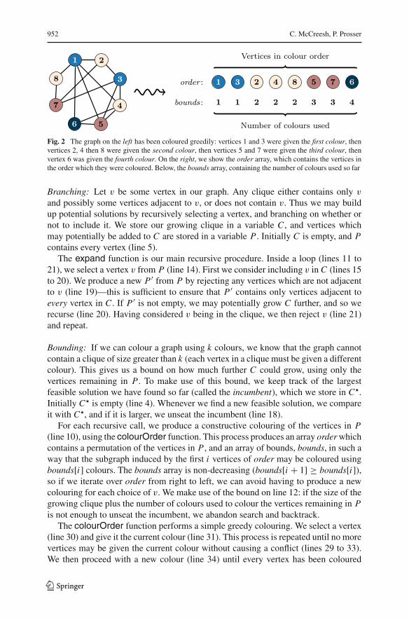
Fig. 2 The graph on the left has been coloured greedily: vertices 1 and 3 were given the first colour, thenvertices 2, 4 then 8 were given the second colour, then vertices 5 and 7 were given the third colour, thenvertex 6 was given the fourth colour. On the right, we show the order array, which contains the vertices inthe order which they were coloured. Below, the bounds array, containing the number of colours used so far
Branching: Let v be some vertex in our graph. Any clique either contains only v
and possibly some vertices adjacent to v, or does not contain v. Thus we may buildup potential solutions by recursively selecting a vertex, and branching on whether ornot to include it. We store our growing clique in a variable C , and vertices whichmay potentially be added to C are stored in a variable P . Initially C is empty, and Pcontains every vertex (line 5).
The expand function is our main recursive procedure. Inside a loop (lines 11 to21), we select a vertex v from P (line 14). First we consider including v in C (lines 15to 20). We produce a new P ′ from P by rejecting any vertices which are not adjacentto v (line 19)—this is sufficient to ensure that P ′ contains only vertices adjacent toevery vertex in C . If P ′ is not empty, we may potentially grow C further, and so werecurse (line 20). Having considered v being in the clique, we then reject v (line 21)and repeat.
Bounding: If we can colour a graph using k colours, we know that the graph cannotcontain a clique of size greater than k (each vertex in a clique must be given a differentcolour). This gives us a bound on how much further C could grow, using only thevertices remaining in P . To make use of this bound, we keep track of the largestfeasible solution we have found so far (called the incumbent), which we store in C�.Initially C� is empty (line 4). Whenever we find a new feasible solution, we compareit with C�, and if it is larger, we unseat the incumbent (line 18).
For each recursive call, we produce a constructive colouring of the vertices in P(line 10), using the colourOrder function. This process produces an array orderwhichcontains a permutation of the vertices in P , and an array of bounds, bounds, in such away that the subgraph induced by the first i vertices of order may be coloured usingbounds[i] colours. The bounds array is non-decreasing (bounds[i + 1] ≥ bounds[i]),so if we iterate over order from right to left, we can avoid having to produce a newcolouring for each choice of v. We make use of the bound on line 12: if the size of thegrowing clique plus the number of colours used to colour the vertices remaining in Pis not enough to unseat the incumbent, we abandon search and backtrack.
The colourOrder function performs a simple greedy colouring. We select a vertex(line 30) and give it the current colour (line 31). This process is repeated until no morevertices may be given the current colour without causing a conflict (lines 29 to 33).We then proceed with a new colour (line 34) until every vertex has been coloured
123

The maximum labelled clique problem 953
(lines 27 to 34). Vertices are placed into the order array in the order in which theywere coloured, and the i th entry of the bounds array contains the number of coloursused at the time the i th vertex in order was coloured. This process is illustrated inFig. 2.
Initial vertex ordering: The order in which vertices are coloured can have a sub-stantial effect upon the colouring produced. Here we will select vertices in a staticnon-increasing degree order. This is done by permuting the graph at the top of search(line 3), so vertices are simply coloured in numerical order. This assists with the bitsetencoding, which we discuss below.
Labels and the budget: So far, what we have described is a variation of a series ofmaximum clique algorithms by Tomita et al. [12–14] (and we refer the reader to thesepapers to justify the vertex ordering and selection rules chosen). Now we discuss howto handle labels and budgets. We are optimising subject to two criteria, so we will takea two-pass approach to finding an optimal solution.
On the first pass (first = true, from line 5), we concentrate on finding the largestfeasible clique, but do not worry about finding the cheapest such clique. To do so, westore the labels currently used in C in the variable L . When we add a vertex v to C ,we create from L a new label set L ′ and add to it any additional labels used (line 16).Now we check whether we have exceeded the budget (line 17), and only proceed withthis value of C if we have not. As well as storing C�, we also keep track of the labelsit uses in L�.
On the second pass (first = false, from line 6), we already have the size of amaximum feasible clique in |C�|, and we seek to either reduce the cost |L�|, or provethat we cannot do so. Thus we repeat the search, starting with our existing values ofC� and L�, but instead of using the budget to filter labels on line 17, we use |L�| − 1(which can become smaller as cheaper solutions are found). We must also change thebound condition slightly: rather than looking only for solutions strictly larger thanC�, we are now looking for solutions with size equal to C� (line 12). Finally, whenpotentially unseating the incumbent (line 18), wemust check to see if eitherC is largerthan C�, or it is the same size but cheaper.
This two-pass approach is used to avoid spending a long time trying to find a cheaperclique of size |C�|, only for this effort to be wasted when a larger clique is found. Theadditional filtering power from having found a clique containing only one additionalvertex is often extremely beneficial. On the other hand, label-based filtering using|L�| − 1 rather than the budget is not possible until we are sure that C� cannot growfurther, since it could be that larger feasible maximum cliques have a higher cost.
Bit parallelism: For the maximum clique problem, San Segundo et al. [10,11]observed that using a bitset encoding for SIMD-like parallelism could speed up animplementation by a factor of between two to twenty, without changing the steps taken.We do the same here: P and L should be bitsets, and the graph should be representedusing an adjacency bitset for each vertex (this representation may be created whenG is permuted, on line 3). Most importantly, the uncoloured and colourable vari-
123

954 C. McCreesh, P. Prosser
ables in colourOrder are also bitsets, and the filtering on line 33 is simply a bitwiseand-with-complement operation.
Note thatC should not be stored as a bitset, to speed up line 16. Instead, it should bean array. Adding a vertex to C on line 15 may be done by appending to the array, andwhen removing a vertex from C on line 21 we simply remove the last element—thisworks because C is used like a stack.
Thread parallelism: Thread parallelism for the maximum clique problem has beenshown to be extremely beneficial [2,5]; we may use an approach previously describedby the authors [5,7] here too. We view the recursive calls to expand as forming a tree,ignore left-to-right dependencies, and explore subtrees in parallel. For work splitting,we initially create subproblems by dividing the tree immediately below the root node(so each subproblem represents a case where |C | = 1 due to a different choice ofvertex). Subproblems are placed onto a queue, and processed by threads in order. Toimprove balance, when the queue is empty and a thread becomes idle, work is thenstolen from the remaining threads by resplitting the final subproblems at distance 2from the root.
There is a single shared incumbent, which must be updated carefully. This may bestored using an atomic, to avoid locking. Care must be taken with updates to ensurethatC� and L� are compared and updated simultaneously—this may be done by usinga large unsigned integer, and allocating the higher order bits to |C�| and the lowerorder bits to the bitwise complement of |L�|.
Note that we are not dividing a fixed amount of work between multiple threads,and so we should not necessarily expect a linear speedup. It is possible that we couldget no speedup at all, due to threads exploring a portion of the search space whichwould be eliminated by the bound during a sequential run, or a speedup greater thanthe number of threads, due to a strong incumbent being found more quickly [3]. Afurther complication is that in the first pass, we could find an equally sized but morecostly incumbent than we would find sequentially. Thus we cannot even guaranteethat this will not cause a slowdown in certain cases [15].
3 Experimental results
We now evaluate an implementation of our sequential and parallel algorithms exper-imentally. Our implementation was coded in C++, and for parallelism, C++11 nativethreads were used. The bitset encoding was used in both cases. Experimental resultsare produced on a desktopmachine with an Intel i5-3570 CPU and 12GBytes of RAM.This is a dual core machine, with hyper-threading, so for parallel results we use fourthreads (but should not expect an ideal-case speedup of 4). Sequential results are froma dedicated sequential implementation, not from a parallel implementation run with asingle thread. Timing results include preprocessing time and thread startup costs, butnot the time taken to read in the graph file and generate random labels.
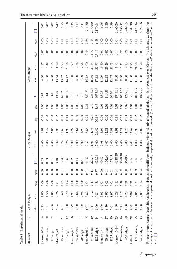
Standard benchmark problems In Table 1 we present results from the same set ofbenchmark instances as Carrabs et al. [1]. These are some of the smaller graphs from
123
The maximum labelled clique problem 955
Table1
Experim
entalresults
Instance
|L|
25%
budg
et50
%budg
et75
%budg
et
size
cost
t seq
t par
[1]
size
cost
t seq
t par
[1]
size
cost
t seq
t par
[1]
john
son8
-2-4
43.13
1.00
0.00
0.00
0.03
4.00
1.87
0.00
0.00
0.02
4.00
1.87
0.00
0.00
0.01
28vertices,
83.51
1.50
0.00
0.00
0.03
4.00
2.48
0.00
0.00
0.01
4.00
2.48
0.00
0.00
0.02
210edges
124.00
2.85
0.00
0.00
0.01
4.00
2.85
0.00
0.00
0.02
4.00
2.85
0.00
0.00
0.02
MANN_a9
115.64
2.76
0.01
0.00
3.18
8.89
5.93
0.02
0.01
13.98
13.34
8.99
0.01
0.00
6.47
45vertices,
216.61
5.60
0.02
0.01
12.43
9.74
10.68
0.08
0.02
46.52
13.32
15.73
0.03
0.01
15.55
918edges
327.00
7.79
0.04
0.01
17.61
10.26
14.99
0.19
0.05
108.13
14.12
23.28
0.03
0.01
13.18
hamming6
-46
3.99
1.97
0.00
0.00
0.32
4.00
1.99
0.00
0.00
0.33
4.00
1.99
0.00
0.00
0.35
64vertices,
114.00
2.64
0.00
0.00
0.43
4.00
2.64
0.00
0.00
0.42
4.00
2.64
0.00
0.00
0.37
704edges
174.00
2.98
0.00
0.00
0.41
4.00
2.98
0.00
0.00
0.43
4.00
2.98
0.00
0.00
0.44
hamming6
-215
6.07
3.82
0.04
0.01
41.32
9.87
7.86
0.76
0.21
382.73
15.42
12.00
2.44
0.66
711.20
64vertices,
297.17
7.12
0.41
0.11
221.77
11.01
14.73
6.25
1.70
2368
.78
15.86
21.84
11.73
3.14
2079
.50
1824
edges
448.00
10.81
1.35
0.37
429.21
12.00
21.49
20.19
5.47
4955
.96
17.13
32.65
23.15
6.28
2170
.84
john
son8
-4-4
145.99
3.93
0.01
0.00
49.82
7.98
6.94
0.02
0.01
85.73
11.09
10.89
0.01
0.00
16.36
70vertices,
276.30
5.95
0.03
0.01
102.60
9.07
12.81
0.02
0.01
110.53
12.18
20.29
0.00
0.00
11.80
1855
edges
407.01
8.97
0.05
0.01
177.13
10.00
19.01
0.02
0.01
60.79
12.97
28.93
0.00
0.00
2.39
john
son1
6-2-4
236.50
5.28
0.15
0.04
4248
.29
8.00
8.91
0.14
0.04
1943
.33
8.00
8.91
0.14
0.04
2066
.26
120vertices,
467.75
11.17
0.29
0.08
5660
.29
8.00
12.21
0.22
0.06
3044
.75
8.00
12.21
0.22
0.06
3290
.52
5460
edges
698.00
14.23
0.28
0.08
3699
.71
8.00
14.23
0.28
0.08
4227
.76
8.00
14.23
0.28
0.08
3909
.15
keller4
286.98
6.89
0.28
0.07
>3h
9.04
12.68
0.10
0.03
>3h
11.00
18.75
0.02
0.01
3304
.30
171vertices,
558.00
12.85
0.32
0.09
>3h
11.00
26.98
0.02
0.01
4081
.97
11.00
26.98
0.02
0.01
4173
.34
9435
edges
839.00
19.82
0.14
0.04
>3h
11.00
31.88
0.02
0.01
4827
.99
11.00
31.88
0.02
0.01
5028
.16
Foreach
graph,weusethreedifferentlabelsetsizes
andthreedifferentbudgets,w
ithrandom
lyallocatedlabels,and
show
averages
over
100runs.Ineach
case,w
eshow
the
averagesize
andcostof
theresult,
thesequ
entia
lrun
timein
second
s,theparalle
lrun
timein
second
s(2
cores,4threads)andthen
the“E
nhanced”
times
repo
rted
byCarrabs
etal.[1]
123
956 C. McCreesh, P. Prosser
the DIMACS implementation challenge,1 with randomly allocated labels. Carrabs etal. used three samples for each measurement, and presented the average; we use onehundred. Note that our CPU is newer than that of Carrabs et al., and we have notattempted to scale their results for a “fair” comparison.
The most significant result is that none of our parallel runtime averages are above7 s, and none of our sequential runtime averages are above 24 s (our worst sequentialruntime from any instance is 32.3 s, and our worst parallel runtime is 8.4 s). This is instark contrast to Carrabs et al., who aborted some of their runs on these instances afterthree hours. Most strikingly, the keller4 instances, which all took Carrabs et al. at leastan hour, took under 0.1 s for our parallel algorithm. We are using a different modelCPU, so results are not directly comparable, but we strongly doubt that hardwaredifferences could contribute to more than one order of magnitude improvement in theruntimes.
We also see that parallelism is in general useful, and is never a penalty, even withvery low runtimes. We see a speedup of between 3 and 4 on the non-trivial instances.This is despite the initial sequential portion of the algorithm, the cost of launchingthe threads, the general complications involved in parallel branch and bound, and thehardware providing only two “real” cores.
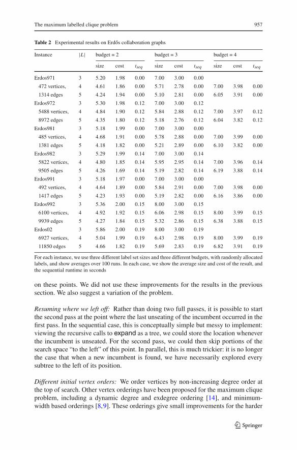
Large sparse graphs In Table 2 we present results using the Erdos collaborationgraphs from the Pajek dataset by Vladimir Batagelj and Andrej Mrvar.2 These arelarge, sparse graphs, with up to 7,000 vertices (representing authors) and 12,000 edges(representing collaborations). We have chosen these datasets because of the potential“social network analysis” application suggested by Carrabs et al., where edge labelsrepresent a particular kind of common interest, and we are looking for a clique usingonly a small number of interests.
For each instance we use 3, 4 and 5 labels, with a budget of 2, 3 and 4. The “3labels, budget 4” cases are omitted, but we include the “3 labels, budget 3” and “4labels, budget 4” cases—although the clique sizes are the same (and are equal to thesize of a maximum unlabelled clique), we see in a few instances the costs do differwhere the budget is 4. Again, we use randomly allocated labels and a sample size of100.
Despite their size, none of these graphs are at all challenging for our algorithm,with average sequential runtimes all being under 0.2 s. However, no benefit at all isgained from parallelism—the runtimes are dominated by the cost of preprocessingand encoding the graph, not the search.
4 Possible improvements and variations
We will briefly describe three possible improvements to the algorithm. These have allbeen implemented and appear to be viable, but for simplicity we do not go into detail
1 http://dimacs.rutgers.edu/Challenges/.2 http://vlado.fmf.uni-lj.si/pub/networks/data/.
123
The maximum labelled clique problem 957
Table 2 Experimental results on Erdos collaboration graphs
Instance |L| budget = 2 budget = 3 budget = 4
size cost tseq size cost tseq size cost tseq
Erdos971 3 5.20 1.98 0.00 7.00 3.00 0.00
472 vertices, 4 4.61 1.86 0.00 5.71 2.78 0.00 7.00 3.98 0.00
1314 edges 5 4.24 1.94 0.00 5.10 2.81 0.00 6.05 3.91 0.00
Erdos972 3 5.30 1.98 0.12 7.00 3.00 0.12
5488 vertices, 4 4.84 1.90 0.12 5.84 2.88 0.12 7.00 3.97 0.12
8972 edges 5 4.35 1.80 0.12 5.18 2.76 0.12 6.04 3.82 0.12
Erdos981 3 5.18 1.99 0.00 7.00 3.00 0.00
485 vertices, 4 4.68 1.91 0.00 5.78 2.88 0.00 7.00 3.99 0.00
1381 edges 5 4.18 1.82 0.00 5.21 2.89 0.00 6.10 3.82 0.00
Erdos982 3 5.29 1.99 0.14 7.00 3.00 0.14
5822 vertices, 4 4.80 1.85 0.14 5.95 2.95 0.14 7.00 3.96 0.14
9505 edges 5 4.26 1.69 0.14 5.19 2.82 0.14 6.19 3.88 0.14
Erdos991 3 5.18 1.97 0.00 7.00 3.00 0.00
492 vertices, 4 4.64 1.89 0.00 5.84 2.91 0.00 7.00 3.98 0.00
1417 edges 5 4.23 1.93 0.00 5.19 2.82 0.00 6.16 3.86 0.00
Erdos992 3 5.36 2.00 0.15 8.00 3.00 0.15
6100 vertices, 4 4.92 1.92 0.15 6.06 2.98 0.15 8.00 3.99 0.15
9939 edges 5 4.27 1.84 0.15 5.32 2.86 0.15 6.38 3.88 0.15
Erdos02 3 5.86 2.00 0.19 8.00 3.00 0.19
6927 vertices, 4 5.04 1.99 0.19 6.43 2.98 0.19 8.00 3.99 0.19
11850 edges 5 4.66 1.82 0.19 5.69 2.83 0.19 6.82 3.91 0.19
For each instance, we use three different label set sizes and three different budgets, with randomly allocatedlabels, and show averages over 100 runs. In each case, we show the average size and cost of the result, andthe sequential runtime in seconds
on these points. We did not use these improvements for the results in the previoussection. We also suggest a variation of the problem.
Resuming where we left off: Rather than doing two full passes, it is possible to startthe second pass at the point where the last unseating of the incumbent occurred in thefirst pass. In the sequential case, this is conceptually simple but messy to implement:viewing the recursive calls to expand as a tree, we could store the location wheneverthe incumbent is unseated. For the second pass, we could then skip portions of thesearch space “to the left” of this point. In parallel, this is much trickier: it is no longerthe case that when a new incumbent is found, we have necessarily explored everysubtree to the left of its position.
Different initial vertex orders: We order vertices by non-increasing degree order atthe top of search. Other vertex orderings have been proposed for the maximum cliqueproblem, including a dynamic degree and exdegree ordering [14], and minimum-width based orderings [8,9]. These orderings give small improvements for the harder
123
958 C. McCreesh, P. Prosser
problem instances when labels are present. However, for the Erdos graphs, dynamicdegree and exdegree orderings were a severe penalty—they are more expensive tocompute (adding almost a whole second to the runtime), and the search space is toosmall for this one-time cost to be ignored.
Reordering colour classes: For the maximum clique problem, small but consistentbenefits can be had by permuting the colour class list produced by colourOrder toplace colour classes containing only a single vertex at the end, so that they are selectedfirst [6]. A similar benefit is obtained by doing this here.
A multi-label variation of the problem: In the formulation by Carrabs et al., eachedge has exactly one label. What if instead edges may have multiple labels? If takingan edge requires paying for all of its labels, this is just a trivial modification to ouralgorithm. But if taking an edge requires selecting and paying for only one of its labels,it is not obvious what the best way to handle this would be. One possibility would beto branch on edges as well as on vertices (but only where none of the available edgesmatches a label which has already been selected).
This modification to the problem could be useful for real-world problems: forCarrabs et al. example where labels represent different relationship types in a socialnetwork graph, it is plausible that two people could both be members of the sameclub and be colleagues. Similarly, for the Erdos datasets, we could use labels eitherfor different journals and conferences, or for different topic areas (combinatorics,graph theory, etc.). When looking for a clique of people using only a small number ofdifferent relationship types, it would make sense to allow only one of the relationshipsto count towards the cost.However,we suspect that this change couldmake the problemsubstantially more challenging.
5 Conclusion
We saw that our dedicated algorithm was faster than a mathematical programmingsolution. This is not surprising. However, the extent of the performance differencewas unexpected: we were able to solve multiple problems in under a tenth of onesecond that previously took over an hour, and we never took more than 10 s to solveany of Carrabs et al.’s instances. We were also able to work with large sparse graphswithout difficulty.
Of course, a more complicated mathematical programming model could close theperformance gap. One possible route, which has been successful for the maximumclique problem in a SAT setting [4], would be to treat colour classes as variables ratherthan vertices. But this would require a pre-processing step, and would lose the “easeof use” benefits of a mathematical programming approach. It is also not obvious howthe label constraints would map to this kind of model, since equivalently colouredvertices are no longer equal.
On the other hand, adapting a dedicated maximum clique algorithm for this prob-lem did not require major changes. It is true that these algorithms are non-trivial toimplement, but there are at least three implementations with publicly available source
123
The maximum labelled clique problem 959
code (one in Java [8] and two with multi-threading support in C++ [2,5]). Also of notewas that bit- and thread-parallelism, which are key contributors to the raw performanceof maximum clique algorithms, were similarly successful in this setting.
A further surprise is that threading is beneficial even with the low runtimes of someproblem instances. We had assumed that our parallel runtimes would be noticeablyworse for extremely easy instances, but this turned out not to be the case. Althoughthere was no benefit for the Erdos collaboration graphs, which were computationallytrivial, for the DIMACS graphs there were clear benefits from parallelism even withsequential runtimes as low as a tenth of a second. For the non-trivial instances, weconsistently obtained speedups of between 3 and 4. Even on inexpensive desktopmachines, it is worth making use of multiple cores.
Acknowledgments This workwas supported by the Engineering and Physical Sciences Research Council[Grant Number EP/K503058/1].
Open Access This article is distributed under the terms of the Creative Commons Attribution Licensewhich permits any use, distribution, and reproduction in any medium, provided the original author(s) andthe source are credited.
References
1. Carrabs, F., Cerulli, R., Dell’Olmo, P.: A mathematical programming approach for the maximumlabeled clique problem. In: Procedia—Social and Behavioral Sciences 108(0), 69–78 (2014). doi:10.1016/j.sbspro.2013.12.821. http://www.sciencedirect.com/science/article/pii/S187704281305461X
2. Depolli, M., Konc, J., Rozman, K., Trobec, R., Janežic, D.: Exact parallel maximum clique algorithmfor general and protein graphs. J. Chem. Inf. Model. 53(9), 2217–2228 (2013). doi:10.1021/ci4002525
3. Lai, T.H., Sahni, S.: Anomalies in parallel branch-and-bound algorithms. Commun. ACM 27(6), 594–602 (1984)
4. Li, C.M., Zhu, Z., Manyà, F., Simon, L.: Minimum satisfiability and its applications. In: Proceedings ofthe Twenty-Second International Joint Conference on Artificial Intelligence, Volume One, IJCAI’11,pp. 605–610. AAAI Press, Palo Alto (2011). doi:10.5591/978-1-57735-516-8/IJCAI11-108
5. McCreesh, C., Prosser, P.: Multi-threading a state-of-the-art maximum clique algorithm. Algorithms6(4), 618–635 (2013). doi:10.3390/a6040618. http://www.mdpi.com/1999-4893/6/4/618
6. McCreesh, C., Prosser, P.: Reducing the branching in a branch and bound algorithm for the maximumclique problem. In: Principles and Practice of Constraint Programming, 20th International Conference,CP 2014. Springer, Berlin (2014)
7. McCreesh, C., Prosser, P.: The shape of the search tree for the maximum clique problem, and theimplications for parallel branch and bound. ACM Trans. Parallel Comput. (2014) (To appear; preprintas CoRR abs/1401.5921)
8. Prosser, P.: Exact algorithms for maximum clique: a computational study. Algorithms 5(4), 545–587(2012). doi:10.3390/a5040545. http://www.mdpi.com/1999-4893/5/4/545
9. San Segundo, P., Lopez, A., Batsyn, M.: Initial sorting of vertices in the maximum clique problemreviewed. In: P.M. Pardalos, M.G. Resende, C. Vogiatzis, J.L. Walteros (eds.) Learning and IntelligentOptimization, Lecture Notes in Computer Science, pp. 111–120. Springer International Publishing(2014). doi:10.1007/978-3-319-09584-4_12
10. San Segundo, P., Matia, F., Rodriguez-Losada, D., Hernando, M.: An improved bit parallel exactmaximum clique algorithm. Optim. Lett. 7(3), 467–479 (2013). doi:10.1007/s11590-011-0431-y
11. San Segundo, P., Rodríguez-Losada, D., Jiménez, A.: An exact bit-parallel algorithm for the maximumclique problem. Comput. Oper. Res. 38(2), 571–581 (2011). doi:10.1016/j.cor.2010.07.019
12. Tomita, E., Kameda, T.: An efficient branch-and-bound algorithm for finding a maximum clique withcomputational experiments. J. Glob. Optim. 37(1), 95–111 (2007)
13. Tomita, E., Seki, T.: An efficient branch-and-bound algorithm for finding a maximum clique. In: Pro-ceedings of the 4th International Conference on Discrete Mathematics and Theoretical Computer Sci-
123
960 C. McCreesh, P. Prosser
ence, DMTCS’03, pp. 278–289. Springer, Berlin (2003). http://dl.acm.org/citation.cfm?id=1783712.1783736
14. Tomita, E., Sutani, Y., Higashi, T., Takahashi, S.,Wakatsuki,M.: A simple and faster branch-and-boundalgorithm for finding a maximum clique. In: Rahman, M., Fujita, S. (eds.) WALCOM: Algorithms andComputation. Lecture Notes in Computer Science, vol. 5942, pp. 191–203. Springer, Berlin (2010).doi:10.1007/978-3-642-11440-3_18
15. Trienekens, H.W.: Parallel branch and bound algorithms. Ph.D. thesis, Erasmus University Rotterdam(1990)
123