Embed Size (px)
Citation preview

HAL Id: inria-00315765https://hal.inria.fr/inria-00315765
Submitted on 30 Aug 2008
HAL is a multi-disciplinary open accessarchive for the deposit and dissemination of sci-entific research documents, whether they are pub-lished or not. The documents may come fromteaching and research institutions in France orabroad, or from public or private research centers.
L’archive ouverte pluridisciplinaire HAL, estdestinée au dépôt et à la diffusion de documentsscientifiques de niveau recherche, publiés ou non,émanant des établissements d’enseignement et derecherche français ou étrangers, des laboratoirespublics ou privés.
A partitioned Newton method for the interaction of afluid and a 3D shell structure
Miguel Angel Fernández, Jean-Frédéric Gerbeau, Antoine Gloria, MarinaVidrascu
To cite this version:Miguel Angel Fernández, Jean-Frédéric Gerbeau, Antoine Gloria, Marina Vidrascu. A partitionedNewton method for the interaction of a fluid and a 3D shell structure. [Research Report] RR-6623,INRIA. 2008, pp.30. inria-00315765

appor t
de r ech er ch e
ISS
N0
24
9-6
39
9IS
RN
INR
IA/R
R--
66
23
--F
R+
EN
G
Thèmes BIO et NUM
INSTITUT NATIONAL DE RECHERCHE EN INFORMATIQUE ET EN AUTOMATIQUE
A partitioned Newton method for the interaction of a
fluid and a 3D shell structure
Miguel A. Fernández — Jean-Frédéric Gerbeau — Antoine Gloria — Marina Vidrascu
N° 6623
August 2008


Centre de recherche INRIA Paris – RocquencourtDomaine de Voluceau, Rocquencourt, BP 105, 78153 Le Chesnay Cedex
Téléphone : +33 1 39 63 55 11 — Télécopie : +33 1 39 63 53 30
A partitioned Newton method for the interaction
of a fluid and a 3D shell structure
Miguel A. Fernández∗ , Jean-Frédéric Gerbeau† , Antoine Gloria‡ ,
Marina Vidrascu§
Thèmes BIO et NUM — Systèmes biologiques et Systèmes numériquesÉquipes-Projets REO & MACS
Rapport de recherche n° 6623 — August 2008 — 30 pages
Abstract: We review various fluid-structure algorithms based on domain de-composition techniques and we propose a new one. The standard methods usedin fluid-structure interaction problems are generally “nonlinear on subdomains”.We propose a scheme based on the principle “linearize first, then decompose”.In other words we extend to fluid-structure problems domain decompositiontechniques classically used in nonlinear elasticity.
Key-words: fluid-structure interaction, Newton algorithm, nonlinear domaindecomposition, 3D shell
∗ Project-team REO, INRIA Paris-Rocquencourt & Paris 6 University† Project-team REO, INRIA Paris-Rocquencourt & Paris 6 University‡ Project-teams MICMAC & REO, ENPC & INRIA Paris-Rocquencourt§ Project-team MACS, INRIA Paris-Rocquencourt
Une méthode de Newton partionnée pour
l’interaction d’un fluide et d’une coque 3D
Résumé : Nous faisons une revue de divers algorithmes de couplage fluide-structure basés sur des techniques de décomposition de domaine et nous enproposons un nouveau. Les méthodes classiques utilisées en interaction fluide-structure sont généralement “non linéaires par sous-domaine”. Nous proposonsun schéma basé sur le principe “linéariser puis décomposer”. En d’autres termes,nous étendons aux problèmes d’interaction fluide-structure des techniques dedécomposition de domaine utilisées classiquement en élasticité non linéaire.
Mots-clés : interaction fluide-structure, algorithme de Newton, décomposi-tion de domaine non linéaire, coque 3D
A partitioned Newton method for the interaction of a fluid and a 3D shell 3
Introduction
In this paper we review various numerical methods to treat the interactionbetween an incompressible fluid and an elastic structure, and we propose a newapproach based on a Newton algorithm and domain decomposition methods.To model the structure, we use 3D-shell elements, which allows us to use threedimensional constitutive laws (see [10, 12, 11]). Up to our knowledge, this isthe first time such elements are used in fluid-structure interaction.
Fluid-structure algorithms are too numerous to be reviewed exhaustively. Aclassification of the various approaches is not obvious either. To begin with,we can consider two groups of methods: the “strongly coupled” and the “looselycoupled” schemes. This distinction is quite clear since it corresponds to a pre-cise property: those schemes which can ensure a well-balanced energy transferbetween the fluid and the structure can be called “strongly coupled”, the otherones are “loosely coupled”. All the methods presented in this study are stronglycoupled. Loosely coupled schemes, which are very powerful in many applicationsbut can be unstable in others, are not considered here. We refer for exampleto [41, 18, 6] for explicit coupling schemes and to [19, 20] for a semi-implicitcoupling scheme.
We can then distinguish “monolithic” and “partitioned” schemes. For exam-ple, an ad hoc solver whose purpose is to solve simultaneously the fluid and thestructure typically leads to a monolithic scheme (see [42, 45, 48, 28, 2, 30, 16, 5],for instance). On the other hand, coupling one fluid solver and one structuresolver as black boxes clearly yields a partitioned scheme. Such a partitionedscheme can be strongly coupled as soon as sub-iterations are performed at eachtime step. The number of subiterations being very large in some application,acceleration techniques have been investigated in several articles: for exampleLe Tallec and Mouro [33] propose a steepest descent approach, Mok et al. [38](see also [31]) propose an Aitken acceleration which is based on the two pre-viously computed solutions, Vierendeels [47] a least-square method which usesseveral previously computed solutions, and Badia et al. [1] an specific linearcombination of the coupling conditions.
It is well-known, in particular since the work by Le Tallec and Mouro [33]and more recently by Deparis et al. [15, 14], that fluid-structure problems canbe tackled with domain decomposition approaches. Indeed, a fluid-structureproblem can be viewed as a general continuum mechanics problem set on onedomain which is split into a fluid part and a structure part. The fluid-structurecoupling conditions then appear as the transmission conditions which ensurethat the solution of the global problem is obtained by “sticking” the two sub-problem solutions. This point of view has been adopted in various studies, eitherwith the so-called “Dirichlet-Neumann” algorithms (see for example [36, 26, 23])or with “Neumann-Neumann” algorithms ([15, 14]).
All these methods have been devised following the rule “apply domain de-composition to the nonlinear global problem and then solve on each subdomainthe nonlinear problems”. On the contrary, in other fields – for example non-linear elasticity [32] – domain decomposition is usually applied with the rule“linearize first, then solve the tangent problem using domain decomposition”.The purpose of this paper is to propose a fluid-structure algorithm based onthe last rule. The resulting algorithm can be viewed as a monolithic schemein the sense that we apply a Newton algorithm to the global fluid-structure
RR n° 6623

4 M.A. Fernández, J.-F. Gerbeau, A. Gloria, M. Vidrascu
problem. But, it is more conform to the practical implementation to considerit as a partitioned scheme, since the fluid and the structure are solved with twodifferent solvers, with their own schemes, and can be run in parallel. Contrarilyto the methods following the first rule, these solvers are only used to solve thetangent problems and to evaluate nonlinear residuals. The use of two differentsolvers has well-known advantages (re-usability of existing codes, flexible choiceof the numerical methods adapted to each sub-problem, etc.). Compared tomonolithic schemes presented in the literature [42, 45, 48, 28, 2, 30, 16, 5], ourapproach may have another advantage: the use of domain decomposition meth-ods to solve the tangent problem is expected to be more efficient than directmethods or iterative methods based on block-preconditioners.
The remainder of the paper is organized as follows. In Section 1 we reviewsome standard approaches to solve fluid-structure interaction problems, in par-ticular those based on domain decomposition arguments, that use the so-calledSteklov-Poincaré operators. In Section 2 we recall the fluid and solid modelsand we set the main notations. In Section 3 we propose a short review onconstitutive laws that have been developed recently to model soft tissues, andin particular the arterial wall. The development of constitutive laws for softtissues is of interest from the numerical point of view. On the one hand, specificfeatures of the model can lead to specific numerical issues such as locking (in-compressibility, thin three dimensional structures) and will motivate the use of3D shell elements. On the other hand, the change of relative complexity of thestructure with respect to the fluid can change the relative efficiency of a methodwith respect to another one. The time scheme is presented in Section 4. In Sec-tion 5 the new algorithm is introduced. We propose in Section 5.3 a simplifiedcomplexity analysis in which compare the efficiency of the proposed algorithmwith other existing approaches. We propose in Section 5.3 a simplified complex-ity analysis whose conclusion may be sum up as follows: the more expensivethe structure problem and nonlinear the fluid (let think of the Navier-Stokesequations but also of complex models for the fluid), the more competitive isexpected this new formulation. Numerical results and a comparison with exist-ing methods are reported in Section 6. Finally, some conclusions are given inSection 7.
1 Classical solution methods
In this section, we briefly review some of the existing algorithms for the nu-merical solution of the nonlinear system arising in the time discretization of thefluid-structure problem with an implicit coupling scheme. These methods aretypically based on the application of a particular nonlinear iterative method tothree different formulations of the nonlinear coupled system.
In general, the time discretization of a fluid-structure problem with an im-plicit coupling scheme leads to a coupled nonlinear problem of the type: Findthe interface displacement γ, the fluid state xf and the solid state xs such that
Formulation (I):
F (xf ,γ) = 0,
S (xs,γ) = 0,
I (xf ,xs) = 0.
(1)
INRIA
A partitioned Newton method for the interaction of a fluid and a 3D shell 5
Equations (1)1 and (1)2 ensure the equilibrium of momentum when the fluidand the solid are subjected to an interface displacement γ, whereas the lastequation enforces the equilibrium of mechanical stresses at the interface.
Problem (1) can be reformulated in terms of γ by eliminating the fluid andsolid unknowns xf ,xs. This yields to the so-called Steklov-Poincaré formula-tion: Find the interface displacement γ such that,
Formulation (II): Sf (γ) + Ss(γ) = 0. (2)
Here, Sf and Ss stand for the fluid and solid Steklov-Poincaré operators whichcan be defined as follows: for a given interface displacement γ, Sf (γ) gives thestress exerted by the fluid on the interface, and analogously for Ss. All thesenotations will be made precise below. In section 4.2, we shall describe the linkbetween (1) and (2).
Finally, the composition of the inverse operator S−1s with (2) gives rise to
the so-called Dirichlet-to-Neumann formulation:
Formulation (III): S−1s
(− Sf (γ)
)− γ = 0. (3)
Formally speaking, Formulations (II) and (III) are similar. Nevertheless, weprefer to distinguish them since they correspond to different approaches in theliterature. The denominations “Dirichlet-Neumann formulation” and “Steklov-Poincaré formulation” are purely conventional (both of them clearly involveSteklov-Poincaré operators).
The three following paragraphs address a brief state-of-the-art on the itera-tive methods for the numerical solution of (1), (2) and (3).
1.1 Monolithic formulation
A common approach in the numerical solution of nonlinear systems, arising inimplicit coupling, consists in applying a Newton based algorithm to the globalformulation (1). This requires the repeated solution of a tangent (or approxi-mated tangent) problem with the following block structure:
DxfF (xf ,γ) 0 Dγ F (xf ,γ)
0 DxsS (xs,γ) Dγ S (xs,γ)
DxfI (xf ,xs) Dxs
I (xf ,xs) 0
δxf
δxs
δγ
= −
F (xf ,γ)S (xs,γ)I (xf ,xs)
.
(4)Newton algorithms based on the numerical solution of (4) in a monolithicfashion, i.e. using global direct or iterative methods, have been reported in[45, 48, 28, 2, 16]. It is worth noticing that such a monolithic approach makesdifficult the use of separate solvers for the fluid and structure sub-problems.Alternatively, system (4) can be solved in a partitioned manner through a block-Gauss elimination of δxf , which leads to the so called block-Newton methods[34, 35, 21, 22].
1.2 Dirichlet to Neumann formulations
Formulation (III) reduces problem (1) to the determination of a fixed point ofthe Dirichlet-to-Neumann operator γ 7→ S−1
s
(−Sf (γ)
). This motivates the use
of fixed-point based methods [33, 39, 38, 37]:
γk+1 = ωkS−1s
(− Sf (γk)
)+ (1− ωk)γk, (5)
RR n° 6623
6 M.A. Fernández, J.-F. Gerbeau, A. Gloria, M. Vidrascu
with ωk a given relaxation parameter which is chosen in order to enhance con-vergence [38, 37, 13, 31]. Alternatively, one can use Newton based methods[26, 23] for a fast convergence towards the solution of (3). This requires thesolution of a tangent problem of the type
(J(γk)− I)δγ = −(S−1
s
(−Sf (γk)
)− γk
), (6)
where J(γ) stands for the Jacobian, or approximated Jacobian [26], of the com-posed operator γ 7→ S−1
s
(− Sf (γ)
). It is worth noticing that exact Jacobian
computations require shape derivative calculus for the fluid [23] (see also [16, 4]).Let us also stress the fact that these methods are naturally partitioned.
1.3 Symmetric Steklov-Poincaré formulation
The Dirichlet-Neumann formulations share a common feature: their implemen-tation is purely sequential. The Steklov-Poincaré formulation (2) may allow toset up parallel algorithms to solve the interface equation.
Following the presentation of Deparis et al. [14], the nonlinear problem (2)can be solved through nonlinear Richardson iterations:
P (γk+1 − γk) = ωk(−Sf (γk)− Ss(γk)), (7)
for an appropriate choice of the preconditioner P , namely
P−1k = αk
[S′
f (γk)]−1
+ (1− αk)[S′
s(γk)]−1
, (8)
where λ 7→ S′f (β)·λ is the differential of Sf at β, and
[S′
f (β)]−1
its inverse. Thischoice generalizes the standard preconditioners of linear domain decompositionmethods (for which S′ = S). If αk is 0, 1 or 0.5 we retrieve, respectively,Dirichlet-Neumann, Neumann-Dirichlet or Neumann-Neumann preconditioners.On the other hand, since equation (2) is nonlinear, one can apply a Newtonmethod, (
S′f (γk) + S′
s(γk))(γk+1 − γk) = −Sf (γk)− Ss(γ
k), (9)
which corresponds to the nonlinear Richardson iteration (7) preconditioned withPk = S′
f (γk) + S′s(γ
k) and ωk = 1. This linear equation can be solved, for ex-ample, by an operator-free GMRES algorithm, with or without preconditioning.For instance, in [14] the authors propose to use the preconditioners (8).
The Newton method applied to the Dirichlet-Neumann formulation is notequivalent to the Newton method applied to the Steklov formulation, since theroles played by the fluid and by the structure are not symmetric in the first ap-proach, whereas they are in the second. After linearization, one cannot compose(6) with Ss to retrieve (9). Finally (8) is not equivalent to (9) since in general(A + B)−1 6= A−1 + B−1.
The advantage of formulation (II) compared to formulation (III) is that thefluid and the structure sub-problems can be solved simultaneously and indepen-dently for the residual computation (right-hand sides of (7)) and the applicationof the preconditioner (S′
f and S′s) as soon as α /∈ 0, 1. However, as we shall see
in section 5.3, a simplified complexity analysis shows that the overall computa-tional costs of both methods might be of the same order, for instance, wheneverthe cost of the fluid sub-problem solution is cheaper.
INRIA
A partitioned Newton method for the interaction of a fluid and a 3D shell 7
The formulations recalled in Sections 1.2 and 1.3 are first based on thecoupling conditions, giving rise to a nonlinear equation on the interface, whichinvolves nonlinear sub-problems. The algorithm we introduce in Section 5 firsttreats the nonlinearity of the whole problem through a Newton method, anduses a Steklov-Poincaré formulation on the tangent problems.
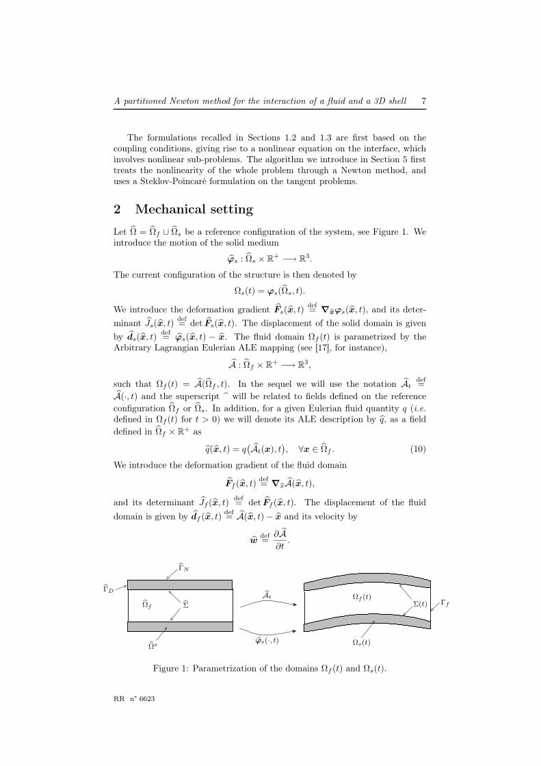
2 Mechanical setting
Let Ω = Ωf ∪ Ωs be a reference configuration of the system, see Figure 1. Weintroduce the motion of the solid medium
ϕs : Ωs × R+ −→ R3.
The current configuration of the structure is then denoted by
Ωs(t) = ϕs(Ωs, t).
We introduce the deformation gradient Fs(x, t)def= ∇bxϕs(x, t), and its deter-
minant Js(x, t)def= det Fs(x, t). The displacement of the solid domain is given
by ds(x, t)def= ϕs(x, t) − x. The fluid domain Ωf (t) is parametrized by the
Arbitrary Lagrangian Eulerian ALE mapping (see [17], for instance),
A : Ωf × R+ −→ R3,
such that Ωf (t) = A(Ωf , t). In the sequel we will use the notation Atdef=
A(·, t) and the superscript will be related to fields defined on the referenceconfiguration Ωf or Ωs. In addition, for a given Eulerian fluid quantity q (i.e.defined in Ωf (t) for t > 0) we will denote its ALE description by q, as a fielddefined in Ωf × R+ as
q(x, t) = q(At(x), t
), ∀x ∈ Ωf . (10)
We introduce the deformation gradient of the fluid domain
Ff (x, t)def= ∇bxA(x, t),
and its determinant Jf (x, t)def= det Ff (x, t). The displacement of the fluid
domain is given by df (x, t)def= A(x, t)− x and its velocity by
wdef=
∂A
∂t.
bΣbΩf
Ωf (t)Σ(t)
Ωs(t)
bAt
bΩsbϕs(·, t)
bΓN
bΓD
Γf
Figure 1: Parametrization of the domains Ωf (t) and Ωs(t).
RR n° 6623
8 M.A. Fernández, J.-F. Gerbeau, A. Gloria, M. Vidrascu
The fluid-structure interface, namely ∂Ωf (t) ∩ ∂Ωs(t) is denoted by Σ(t),and Γf = ∂Ωf (t)\Σ(t) stands for the portion of the fluid boundary that isnot shared with the boundary of the structure. The surface Γf is assumed tobe independent of t. The boundary ∂Ωs of the reference configuration for thestructure is divided into three disjoint parts ΓD, ΓN and Σ, with Σ(t) = At(Σ).We denote by n the outward unit normal on the fluid boundary in the currentconfiguration, and by ns the outward unit normal on the reference structureboundary.
2.1 The coupled problem
We consider an homogeneous, Newtonian viscous, incompressible fluid with den-sity ρf and dynamic viscosity µ. Its state is described by its Eulerian velocityu and pressure p. The constitutive law for the Cauchy stress tensor is given bythe following expression:
σ(u, p) = −pI + 2µǫ(u),
with ǫ(u)def=[∇u + (∇u)T
]/2. In absence of body forces, these unknowns
satisfy the incompressible Navier-Stokes equations in an ALE formulation:
ρf
∂u
∂t
∣∣∣bx
+ ρf (u−w) ·∇u− div(2µǫ(u)
)+ ∇p = 0, in Ωf (t),
div u = 0, in Ωf (t),
σ(u, p) · n = g, on Γf ,
(11)
where∂
∂t
∣∣∣bx
stands for the ALE time derivative, wdef= w A−1
t , and g a given
density of surface force.The structure is supposed to be hyperelastic under large displacements and
deformations. Its density is denoted by ρs. Its state is described by its dis-placement ds and its first Piola-Kirchoff stress tensor T . The latter is relatedto ds as the gradient of an internal stored energy function W (Fs). The choiceof the internal stored energy will depend on the problem under considerationand will not change the setting of the fluid-structure problem. Assuming thatthe structure is clamped on ΓD and under no body and surface forces, theseunknowns are driven by the following elastodynamic equations
Jsρs
∂2ds
∂t2− div bxT = 0, in Ωs,
d = 0, on ΓD,
T · ns = 0, on ΓN .
(12)
The coupling between the solid and the fluid, namely equations (11) and(12), is realized through standard boundary conditions at the fluid-structureinterface Σ(t) that ensure the balance of the mechanical energy over the wholedomain. This is achieved by imposing three interface conditions:
• A geometrical condition enforcing the matching between ϕs and A on theinterface
df = ds, on Σ. (13)
INRIA
A partitioned Newton method for the interaction of a fluid and a 3D shell 9
Inside Ωf , the fluid domain displacement df can be defined as an arbitrary(suitable) extension of ds over the domain Ωf , namely,
df = Ext(ds|bΣ) (14)
(see Remark 1 below).
• A kinematic condition enforcing the continuity of the velocities at theinterface
u =∂ds
∂t A−1
t , on Σ(t). (15)
• And a kinetic condition imposing the stress continuity at the interface
T ns = −Jf σ(u, p)F−Tf n, on Σ. (16)
To summarize, the fluid-structure system involving an incompressible viscousfluid and a hyperelastic structure is described in terms of the unknowns (u, p, df , ds)satisfying the coupled problem (11)-(16).
Remark 1 In practice, we can choose as operator Ext a harmonic extensionoperator, by solving a Laplace equation
−div (κ∇df ) = 0, on Ωf ,
df = ds, on Σ,
df = 0, on Γf ,
(17)
where κ > 0 is a given “diffusion” coefficient, that can depend on ds. Otheralternative extension approaches can be found, for instance, in [3, 46].
Remark 2 The combination of (13) and (15) enforces u = w on Σ(t). Thisrequirement is not strictly necessary but simplifies the construction of the ALE
map. In general we could replace (14) by∂ds
∂t A−1
t · n = w · n on Σ(t).
Remark 3 For simplicity, we have only prescribed Neumann boundary condi-tions in (11). In practice we may use Dirichlet conditions on some part of theboundary.
2.2 Weak formulation
Problem (11)-(16) can be reformulated in a weak variational form using appro-priate test functions, performing integrations by parts and taking into accountthe boundary and interface conditions.
In what follows, we will make explicit the dependence of Ωf (t) and Σ(t) ondf by introducing the notations
Ωf (df )def= Ωf (t), Σ(df )
def= Σ(t).
RR n° 6623
10 M.A. Fernández, J.-F. Gerbeau, A. Gloria, M. Vidrascu
Let (vf , q) ∈ [H1(Ωf )]3 × L2(Ωf ), multiplying the fluid problem (11) by(vf , q) = (vf A
−1t , q A−1
t ) integrating over Ωf (df ) and after integrations byparts we get
d
dt
∫
Ωf (cdf )
ρfu · vf dx +
∫
Ωf (cdf )
div[ρfu⊗
(u−w
(df
))]· vf dx
+
∫
Ωf (cdf )
σ(u, p) : ∇vf dx−
∫
Σ(cdf )
σ(u, p) · vf · n
da−
∫
Γin−out
g · vf da−
∫
Ωf (cdf )
q div u dx = 0,
where
w(df
)=
∂df
∂t A−1
t .
For the structure, multiplying (12) by vs ∈ [H1ΓD
(Ωs)]3, integrating by parts
over Ωs, one gets
∫
bΩs
ρ0∂2ds
∂t2· vs dx+
∫
bΩs
∂W
∂F(I+∇ds) : ∇vs dx−
∫
bΣ
∂W
∂F(I+∇ds)ns · vs da = 0,
where ρ0 = Jsρs. Therefore, taking into account the coupling condition (16), itfollows that
d
dt
∫
Ωf (cdf )
ρfu · vf dx +
∫
Ωf (cdf )
div[ρfu⊗
(u−w
(df
))]· vf dx
+
∫
Ωf (cdf )
σ(u, p) : ∇vf dx−
∫
Γin−out
g · vf da−
∫
Ωf (cdf )
q div u dx
+
∫
bΩs
ρ0∂2ds
∂t2· vs dx +
∫
bΩs
∂W
∂F(I +∇ds) : ∇vs dx = 0, (18)
for all (vf , q) ∈ [H1(Ωf )]3 × L2(Ωf ) and vs ∈ [H1ΓD
(Ωs)]3 with vf = vs on Σ.
The weak form of the geometry coupling conditions (13) and (14) are rewrittenin terms of the interface displacement γ ∈ [H
12 (Σ)]3 as
∫
bΩf
(df − Ext(γ)
)· τ dx +
∫
bΣ
(ds − γ) · ζ da = 0, (19)
for all τ ∈ [L2(Ωf )]3 and ζ ∈ [L2(Σ)]3. Finally, the continuity of the velocitiesat the interface (15) is reformulated as
∫
bΣ
(u− w(df )
)· ξ da = 0, (20)
for all ξ ∈ [L2(Σ)]3.Therefore, after summation of (18)-(20) we obtain the following global weak
formulation of problem (11)-(16): Find u : Ωf × R+ → R3, p : Ωf × R+ → R,
INRIA
A partitioned Newton method for the interaction of a fluid and a 3D shell 11
df : Ωf × R+ → R3, ds : Ωs × R+ → R3 and γ : Σ× R+ → R3 such that
d
dt
∫
Ωf (cdf )
ρfu · vf dx +
∫
Ωf (cdf )
div[ρfu⊗
(u−w
(df
))]· vf dx
+
∫
Ωf (cdf )
σ(u, p) : ∇vf dx−
∫
Γin−out
g · vf da−
∫
Ωf (cdf )
q div u dx
+
∫
bΩs
ρ0∂2ds
∂t2· vs dx +
∫
bΩs
∂W
∂F(I +∇ds) : ∇vs dx +
∫
bΩf
(df − Ext(γ)
)· τ dx
+
∫
bΣ
(ds − γ) · ζ da +
∫
bΣ
(u− w(df )
)· ξ da = 0, (21)
with u(·, t) = u(·, t)A−1t , p(·, t) = p(·, t)A−1
t , and for all (vf , q) ∈ [H1(Ωf )]3×
L2(Ωf ), vs ∈ [H1ΓD
(Ωs)]3 with vf = vs on Σ, τ ∈ [L2(Ωf )]3, ζ ∈ [L2(Σ)]3 and
ξ ∈ [L2(Σ)]3.
3 Constitutive laws for artery walls
3.1 Three dimensional constitutive laws
In an extensive survey article [29], Holzapfel et al. have analyzed and comparedexisting constitutive models for arterial walls. They have also introduced a newframework to take into account anisotropy and various mechanical effects suchas inflation and torsion. Their model is based on a thick-walled nonlinearlyelastic tube consisting of two layers. Another model has been introduced byvan Oijen in his PhD thesis [40]. More microscopically based, it uses the mixingtheory to take into account the fibers in the layers. Even more precise at themicroscopic level, Caillerie et al. have introduced a nonlinear homogenizationapproach to fiber-reinforcement in soft tissues ([7]).
These three models have two common features: they are three-dimensionaland anisotropic. Previous approaches, such as the Fung model in [25], are basedon geometrical simplifications, such as membrane, and more generally on thinshell. However, as pointed out in [29], such simplifications are not suitable forthe analysis of the through-thickness stress distribution in an artery or for thetreatment of shearing deformations. In addition, the combination of inflationand torsion effects cannot be reproduced by such simplified models. This mayexplain why three-dimensional constitutive laws are needed to correctly handlethe passive mechanical behavior of artery walls.
From a physiological point of view, the arterial wall is made of three lay-ers (the intima, the media and the adventitia). For a healthy artery, only themedia and the adventitia have a significant mechanical role. In addition, theirmechanical behavior is highly anisotropic due to the presence of fibers (collage-nous components). In [29], Holzapfel et al. propose a model based on twolayers modeling the media and the adventitia. For both layers, the materialis supposed to be three-dimensional, thin, hyperelastic, in finite deformation,incompressible, anisotropic (in the fiber directions) and pre-stressed.
The elastic assumption is well satisfied in some vessels, as the aorta, theiliac and carotid arteries. For other arteries, including the femoral, celiac andcerebral arteries, viscoelastic models are needed.
RR n° 6623
12 M.A. Fernández, J.-F. Gerbeau, A. Gloria, M. Vidrascu
As a consequence of the above assumptions, the free energy of a layer canbe written as
W (Fs) = Ψiso(I1, I2, J) + Ψfib(I4, I5), (22)
where Fs is the deformation gradient, I1, I2 and J its three principal invariantsand I4 and I5 its pseudo-invariants related to the reinforcement direction. Thefirst part of the energy Ψiso is isotropic, typically a neo-Hookean, Mooney-Rivlinor Ciarlet-Geymonat type of energy. The second part Ψfib is anisotropic andinvolves an exponential term in order to reproduce the strong stiffening effectof each layer at high pressure.
From a computational point of view, the above combination of mechanicalproperties gives rise to two major difficulties: the treatment of incompressibilityin finite deformation and the treatment of bad aspect ratios for thin three-dimen-sional structures. Both phenomena lead to locking problems ([9],[12]) if not cor-rectly treated. Incompressibility issues are classically dealt with using a mixedfinite element method, whereas locking phenomena in thin three-dimensionalstructures are treated using re-interpolation techniques [10, 12, 11] as presentedin the following subsection.
3.2 3D shell elements
A general structural model of the blood flow with complex and realistic geome-tries has to be three-dimensional and handle large displacements.
Since the wall of the blood vessels is thin, it is convenient to use shell ele-ments; they accurately describe its geometry. All finite elements adopted in oursimulations are general shell elements. Previously, Gerbeau et al. have used theMITC4 elements [26, 27] with a 3D constitutive law for which the transversalstress is null and a kinematic constraint is needed to make the model compatiblewith a Reissner-Mindlin shell model. This restricts the choice of the energy.
We consider here 3D-shell elements [10, 12, 11]. These elements appear asstandard three-dimensional elements. Thus it is very easy to couple them toother three-dimensional formulations through the nodes on the faces. The ele-ment considered here, called MI3D, uses standard 3D Q2 shape functions. Theadvantage of a quadratic approximation in the shell’s thickness is that it ispossible to deal with standard 3D energies, such as generalized Hook or any hy-perelastic stored energy, defined by using the Cauchy-Green tensor’s invariants,such as the one defined in (22).
In order to be able to apply MITC techniques to stabilize the formulation, itis necessary to compute the first and second derivatives of the stored energy withrespect to the Green-Lagrange tensor, defined hereafter, in local coordinates(r, s, z), as it is usually done in shell element (see Figure 2):
eij(~U)def=
1
2(~gi · ~U,j + ~gj · ~U,i + ~U,i · ~U,j), (23)
where ~gi is a covariant basis.
INRIA
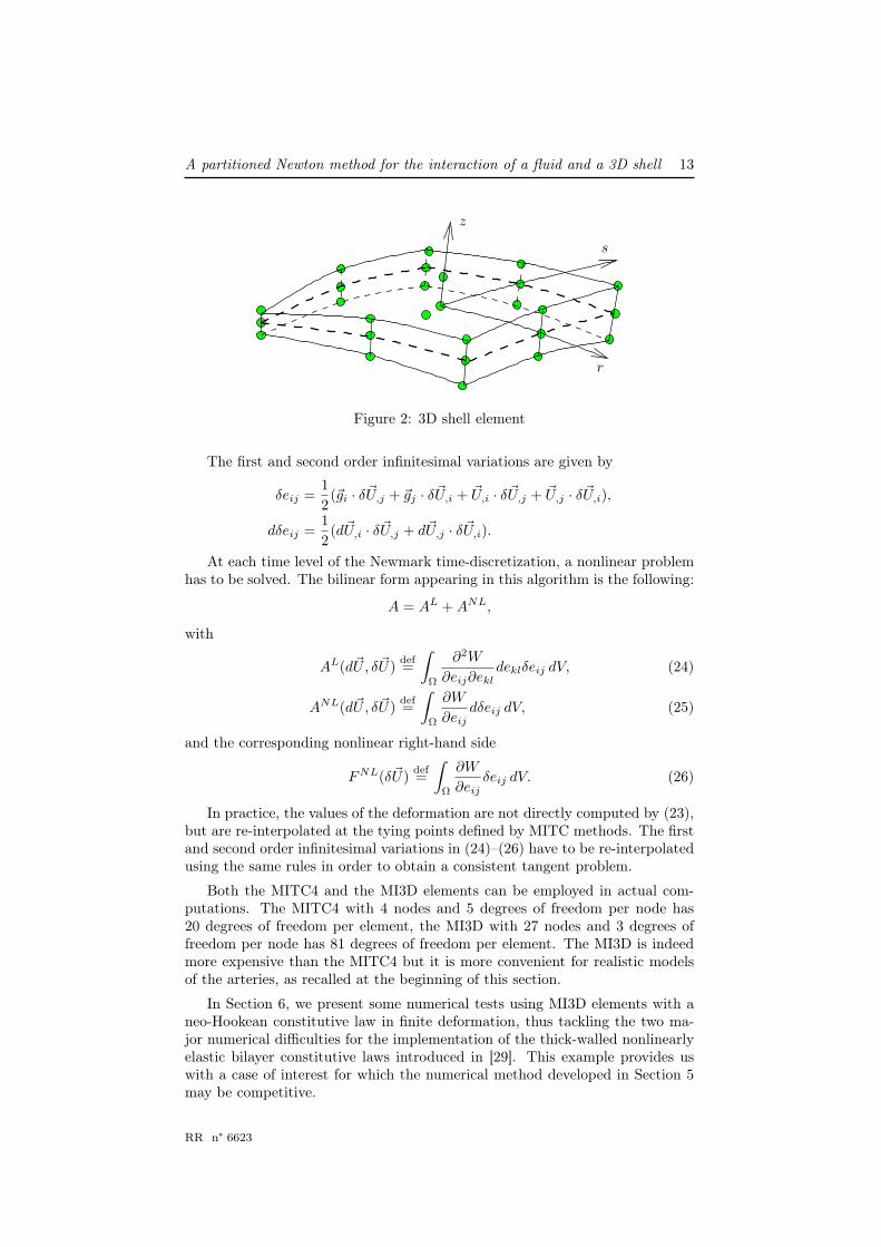
A partitioned Newton method for the interaction of a fluid and a 3D shell 13
r
z
s
Figure 2: 3D shell element
The first and second order infinitesimal variations are given by
δeij =1
2(~gi · δ~U,j + ~gj · δ~U,i + ~U,i · δ~U,j + ~U,j · δ~U,i),
dδeij =1
2(d~U,i · δ~U,j + d~U,j · δ~U,i).
At each time level of the Newmark time-discretization, a nonlinear problemhas to be solved. The bilinear form appearing in this algorithm is the following:
A = AL + ANL,
with
AL(d~U, δ~U)def=
∫
Ω
∂2W
∂eij∂ekl
deklδeij dV, (24)
ANL(d~U, δ~U)def=
∫
Ω
∂W
∂eij
dδeij dV, (25)
and the corresponding nonlinear right-hand side
FNL(δ~U)def=
∫
Ω
∂W
∂eij
δeij dV. (26)
In practice, the values of the deformation are not directly computed by (23),but are re-interpolated at the tying points defined by MITC methods. The firstand second order infinitesimal variations in (24)–(26) have to be re-interpolatedusing the same rules in order to obtain a consistent tangent problem.
Both the MITC4 and the MI3D elements can be employed in actual com-putations. The MITC4 with 4 nodes and 5 degrees of freedom per node has20 degrees of freedom per element, the MI3D with 27 nodes and 3 degrees offreedom per node has 81 degrees of freedom per element. The MI3D is indeedmore expensive than the MITC4 but it is more convenient for realistic modelsof the arteries, as recalled at the beginning of this section.
In Section 6, we present some numerical tests using MI3D elements with aneo-Hookean constitutive law in finite deformation, thus tackling the two ma-jor numerical difficulties for the implementation of the thick-walled nonlinearlyelastic bilayer constitutive laws introduced in [29]. This example provides uswith a case of interest for which the numerical method developed in Section 5may be competitive.
RR n° 6623

14 M.A. Fernández, J.-F. Gerbeau, A. Gloria, M. Vidrascu
4 Semi-discretized weak formulation
In this section, the weak coupled formulation (21) is semi-discretized in timeusing an implicit coupling-scheme. The resulting nonlinear problem will beturned into an abstract form. This will allow us to introduce in the next sectiongeneral nonlinear iterative solution methods.
4.1 Implicit coupling scheme
We use an implicit Euler scheme for the ALE Navier-Stokes equations, witha semi-implicit treatment of the nonlinear convective term. Furthermore weuse a mid-point rule for the structural equation. Thus, given a time step δt >0, for n = 0, 1, . . ., the time semi-discretized coupled problem writes: Given(un, pn, df
n, ds
n,γn
), find
(un+1, pn+1, df
n+1, ds
n+1,γn+1
)∈ [H1(Ωf )]3 × L2(Ωf )× [H1(Ωf )]3
× [H1(Ωs)]3 × [H
12 (Σ)]3,
such that
1
δt
∫
Ωf ( bdn+1
f)
ρfun+1 · vf dx−1
δt
∫
Ωf ( bdnf)
ρfun · vf dx
+
∫
Ωf ( bdn+1
f)
σ(un+1, pn+1) : ∇vf dx
+
∫
Ωf ( bdn+1
f)
div[ρfun+1 ⊗
(un −w
(df
n+1))]· vf dx
−
∫
Γin−out
gn+1 ·vf da−
∫
Ωf ( bdn+1
f)
q div un+1 dx+
∫
bΩf
(dn+1
f − Ext(γn+1
))·τ dx
+
∫
bΣ
(un+1 − w
(dn+1
f
))· ξ da +
2
δt2
∫
bΩs
ρ0dn+1s · vs dx
−2
δt2
∫
bΩs
ρ0
(dn
s + ∆t˙
dns
)· vs dx +
∫
bΩs
∂W
∂F
(I +
1
2∇(dn
s + dn+1s )
): ∇vs dx
+
∫
bΣ
(dn+1
s − γn+1)· ζ da = 0, (27)
for all (vf , q, ξ, τ , ζ, vs) ∈ [H1(Ωf )]3×L2(Ωf )×[L2(Σ)]3×[L2(Ωf )]3×[L2(Σ)]3×
[H1ΓD
(Ωs)]3 such that vf = vs on Σ, and with un = un(I+df
n)−1 (analogously
for pn) and ˙dn+1
s =2
δt
(dn+1
s − dns
)−
˙dn
s .
4.2 Abstract formulations
Problem (27) can be rewritten in a more compact form in terms of the fluid,solid and interface state operators. This is the aim of the following paragraphs.
INRIA
A partitioned Newton method for the interaction of a fluid and a 3D shell 15
Based on the discrete weak formulation (27) we introduce the fluid operator
F : [H1(Ωf )]3 × L2(Ωf )× [H1(Ωf )]3 × [H12 (Σ)]3
−→([H1
bΣ(Ωf )]3 × L2(Ωf )× [L2(Σ)]3 × [L2(Ωf )]3
)′,
defined by
⟨F(u, p, df ,γ
),(vf , q, ξ, τ
)⟩=
1
∆t
∫
Ωf ( bdf )
ρfu · vf dx
−1
∆t
∫
Ωf ( bdnf)
ρfun · vf dx
+
∫
Ωf ( bdf )
div[ρfu⊗
(un −w
(df
))]· vf dx
+
∫
ΩF ( bdf )
σ(u, p) : ∇vf dx−
∫
Γin−out( bdf )
gn+1 · vf da
−
∫
Ωf ( bdf )
q div u dx +
∫
bΣ
(u− w
(df
))· ξ da
+
∫
bΩf
(df − Ext(γ)
)· τ dx,
(28)
for all (vf , q, ξ, τ ) ∈ [H1(Ωf )]3 × L2(Ωf )× [L2(Σ)]3 × [L2(Ωf )]3.Analogously, from (27), the solid operator
S : [H1(Ωs)]3 × [H
12 (Σ)]3 −→ ([H1
ΓD∪bΣ(Ωs)]
3 × [L2(Σ)]3)′,
is given by
⟨S(ds,γ), (vs, ζ)
⟩=
2
δt2
∫
bΩs
ρ0ds · vs dx−2
δt2
∫
bΩs
ρ0
(dn
s + δt˙
dns
)· vs dx
+
∫
bΩs
∂W
∂F
(I +
1
2∇(dn
s + ds
)): ∇vs dx +
∫
bΣ
(ds − γ) · ζ da,
(29)
for all (vs, ζ) ∈ [H1ΓD
(Ωs)]3 × [L2(Σ)]3.
Finally, letLf : [H
12 (Σ)]3 → [H1
Γin−out(Ωf )]3
andLs : [H
12 (Σ)]3 → [H1
∂ bΩs\bΣ(Ωs)]
3
be two given continuous linear lift operators. The interface operator
I : [H1(Ωf )]3 × L2(Ωf )× [H1(Ωf )]3 × [H1(Ωs)]3 −→ [H− 1
2 (Σ)]3,
is then defined by⟨I(u, p, df , ds
),µ⟩
=⟨F(u, p, df ,γ
), (Lfµ, 0,0,0)
⟩+⟨S(ds,γ
), (Lsµ,0)
⟩,
(30)for all µ ∈ [H
12 (Σ)]3.
RR n° 6623

16 M.A. Fernández, J.-F. Gerbeau, A. Gloria, M. Vidrascu
Remark 4 The interface operator does not depend on γ since, due to the choiceof the test functions, the terms involving γ vanish in the right-hand side of (30).
According to the above definitions, problem (27) is equivalent to
Formulation (I):
F(un+1, pn+1, dn+1
f ,γn+1)
= 0,
S(dn+1
s ,γn+1)
= 0,
I(un+1, pn+1, dn+1
f , dn+1s
)= 0.
(31)
4.3 Steklov-Poincaré operators
In order to describe partitioned methods for the numerical solution of (27), wenow introduce the nonlinear fluid and solid Steklov-Poincaré operators.
The nonlinear fluid Steklov-Poincaré operator
Sf : [H12 (Σ)]3 −→ [H− 1
2 (Σ)]3,
is defined by
〈Sf (γ),µ〉 =⟨I(u(γ), p(γ), df (γ),0
),µ⟩
,
for all γ,µ ∈ [H12 (Σ)]3, where (u(γ), p(γ), df (γ)
)is the solution of the Dirichlet
fluid problem:
F(u(γ), p(γ), df (γ),γ
)= 0.
In an analogous way, we introduce the nonlinear solid Steklov-Poincaré operator
Ss : [H12 (Σ)]3 −→ [H− 1
2 (Σ)]3,
given by ⟨Ss(γ),µ
⟩=⟨I(0, 0,0, ds(γ)
),µ⟩
,
for all γ,µ ∈ [H12 (Σ)]3 and where ds(γ) is the solution of the Dirichlet solid
problem:
S(ds(γ),γ
)= 0.
From the above definitions, it follows that problem (27) (or (31)) is equivalentto
Formulation (II): Sf (γ) + Ss(γ) = 0. (32)
The composition of (32) with the inverse operators S−1s gives rise to the Dirichlet-
to-Neumann formulation, namely
Formulation (III): S−1s
(− Sf (γ)
)− γ = 0. (33)
We could also consider the Neumann-to-Dirichlet formulation
S−1f
(− Ss(γ)
)− γ = 0
by composing (32) with S−1f . Nevertheless it is rarely used in practice and it is
known to lead to poor algorithms in some cases, as pointed out in [8].
INRIA

A partitioned Newton method for the interaction of a fluid and a 3D shell 17
5 A partitioned Newton method
In what follows, we skip the upper script n since the time step is fixed. Themethod presented here consists in solving (31) by a Newton method: given an
initial guess (u0, p0, df
0, ds
0,γ0), the algorithm reads
1. Evaluate the nonlinear residual of problem (31).
2. Solve the tangent problem (see (37) below) by a domain decompositionmethod.
3. Update solution:(u, p, df , ds,γ
)←(u, p, df , ds,γ
)+(δu, δp, δdf , δds, δγ
).
4. repeat until convergence.
Compared to the known fluid-structure algorithms presented in Section 1.3, thispartitioned Newton method amounts to switching the domain decompositionand the linearization in the resolution of the coupled problem. We provide thetangent problem in the following sections, as well as details for the domaindecomposition resolution.
5.1 Weak state operators derivatives
In this section, we present the differentiation of the fluid, structure and interfaceoperators of Section 4.2 with respect to their arguments. This derivation usesshape derivative calculus for the differentiation of integral terms with respectto their supports. We refer the reader to [23] where this issue is addressed (seealso [16, 4]).
The linearized fluid operator at state (u, p, df ,γ) ∈ [H1(Ωf )]3 × L2(Ωf ) ×
[H1(Ωf )]3 × [H12 (Σ)]3 is denoted by
DF(u, p, df ,γ) : [H1(Ωf )]3 × L2(Ωf )× [H1(Ωf )]3 × [H12 (Σ)]3 −→
([H1
bΣ(Ωf )]3 × L2(Ωf )× [L2(Σ)]3 × [L2(Ωf )]3
)′,
RR n° 6623

18 M.A. Fernández, J.-F. Gerbeau, A. Gloria, M. Vidrascu
and is given by
〈DF(u, p, df ,γ) · (δu, δp, δdf , δγ), (vf , q, ξ, τ )〉
=
∫
ΩF (cdf )
div[ρfδu⊗ (un −w(df ))
]· vf dx
+
∫
ΩF (cdf )
σ(δu, δp) : ∇vf dx
−
∫
ΩF (cdf )
q div δu dx +1
∆t
∫
ΩF (cdf )
(div δdf )ρfu · vf dx
+
∫
ΩF (cdf )
div
ρfu⊗ (un −w(df ))[I div δdf − (∇δdf )T
]· vf dx
−1
∆t
∫
ΩF (cdf )
div(ρfu⊗ δdf ) · vf dx
+
∫
ΩF (cdf )
σ(u, p)[I div δdf − (∇δdf )T
]: ∇vf dx
−
∫
ΩF (cdf )
µ[∇u∇δdf + (∇δdf )T(∇u)T
]: ∇vf dx
−
∫
ΩF (cdf )
q div
u[I div δdf − (∇δdf )T
]dx +
∫
bΣ
(δu−
δdf
∆t
)· ξ da
+ρ
∆t
∫
ΩF (cdf )
δu · vf dx +
∫
bΩF
(δdf − Ext(δγ)) · τ dx
(34)
for all (vf , q, ξ, τ ) ∈ [H1(Ωf )]3 × L2(Ωf )× [L2(Σ)]3 × [L2(Ωf )]3.The linearized solid operator at state (ds,γ) ∈ [H1
ΓD(Ωs)]
3 × [L2(Σ)]3
DS(ds,γ) : [H1ΓD
(Ωs)]3 × [H
12 (Σ)]3 −→ ([H1
ΓD∪bΣ(Ωs)]
3 × [L2(Σ)]3)′,
is given by
〈DS(ds,γ) · (δds, δγ), (vs, ζ)〉 =2
(∆t)2
∫
bΩS
ρ0δds · vs dx
+1
2
∫
bΩS
∇δds :
(∂2W
∂F 2(I +∇ds)
): ∇vs dx +
∫
bΣ
(δds − δγ) · ζ da, (35)
for all (vs, ζ) ∈ [H1ΓD
(Ωs)]3 × [L2(Σ)]3.
We finally introduce the linearized interface operator at state (u, p, df , ds)
D I(u, p, df , ds) : [H1(Ωf )]3×L2(Ωf )× [H1(Ωf )]3× [H1(Ωs)]3 −→ [H− 1
2 (Σ)]3,
defined by
⟨D I(u, p, df , ds) ·
(δu, δp, δdf , δds
),µ⟩
=⟨DF
(u, p, df ,0
)·(δu, δp, δdf ,0
), (Lfµ, 0,0,0)
⟩
+⟨DS
(ds,0
)(δds,0
), (Lsµ,0)
⟩, (36)
INRIA
A partitioned Newton method for the interaction of a fluid and a 3D shell 19
for all µ ∈ [H12 (Σ)]3.
In terms of the operators defined above, the tangent problem associated with(31) reads
DF(u, p, df ,γ
)·(δu, δp, δdf , δγ
)= −F
(u, p, df ,γ
),
DS(ds,γ
)·(δds, δγ
)= −S
(ds,γ
),
D I(u, p, df , ds
)·(δu, δp, δdf , δds
)= −I
(u, p, df , ds
).
(37)
Once the linear fluid, solid and interface operators DF , DS and D I aredefined, we can introduce the linear Steklov-Poincaré operators SF,l and SS,l
using the formula of Section 4.3 with the linearized operators instead of thenonlinear operators. It may be noticed that the linear Steklov-Poincaré oper-ators are different from the linearization of the nonlinear Steklov operators ofSection 4.3.
5.2 Implementation issues
In this subsection, we briefly describe the general domain decomposition al-gorithm used to solve the linear problems introduced above, namely both theDirichlet-Neumann and the Neumann-Neumann algorithms (in Table 1).
General algorithm.
Following the practical implementation, we decompose the algorithm accordingto three distinct solvers: the master (which, roughly speaking, solves the thirdequation of (37) by a GMRES method), the fluid solver (which solves the firstequation of (37)) and the solid solver (which solves the second equation of (37)).
The iterative algorithm is as follows:
1. Evaluate the Newton residual (right-hand sides of (37)).
2. Initialization of the Domain Decomposition method:
(a) Lifting of the external load and boundary conditions, that is solvethe first and second equations of (37) with δγ = 0.
(b) Computation of the right-hand side of the Schur complement by themaster, insert the residuals received from the fluid and from the solidinto (36) and the third equation of (37). This step evaluates how farthe solution with zero on the interface is from the true solution ofthe coupled problem (37).
(c) Preconditioning the right-hand side of the Schur complement.
3. Iteration until convergence of the GMRES algorithm on the Schur com-plement by the master, which updates the displacement δγ, sends it tothe fluid and solid solvers in order to
(a) Evaluate the new residual
(b) Preconditioning the residual
RR n° 6623
20 M.A. Fernández, J.-F. Gerbeau, A. Gloria, M. Vidrascu
4. End of the domain decomposition algorithm.
The detailed description of these steps for both the Dirichlet-Neumann andNeumann-Neumann algorithms is given in Table 1, which is commented in thefollowing two paragraphs. Note that the steps (2a) and (4) do not depend onthe preconditioner.
Dirichlet-Neumann preconditioner
The Dirichlet-Neumann preconditioner amounts to preconditioning the Schurcomplement using the solid problem only, namely the exact tangent problemof the solid (second equation of (37)) with Neumann boundary conditions. Itis worth noticing that the preconditioning step is not performed in parallelsince only the structure problem is used to precondition the residual. For eachiteration (3) of the GMRES algorithm on the Schur complement, the mastersends δγ in Step (3a) to the fluid solver only, which performs the instructionsof Table 1 and returns a residual to the master. In Step (3b), the master sendsthis residual to the solid solver, which applies the preconditioner according toTable 1 and returns a displacement δγ. The master then sums the displacements12 (δγ + δγ) and computes a new displacement using the update formula of theGMRES algorithm. At convergence, the final value of δγ is known and thesolutions in the fluid and in the solid are computed as indicated in Table 1.
Let us point out that the Dirichlet-Neumann algorithm described above is apurely sequential algorithm.
Neumann-Neumann preconditioner
The Neumann-Neumann preconditioner uses both the tangent fluid problem andthe tangent solid problem (first and second equations of (37)) with Neumannboundary conditions. This algorithm is fully parallel since both the precon-ditioning steps (2c) and (3b) and residual evaluation steps (3a) can be donesimultaneously by the fluid and solid solvers. Although for the tangent solidproblem, considering Neumann boundary conditions is standard, for the tan-gent fluid problem this is not the case. In particular, shape derivative terms(that depend on the lifting w(δdf ) of the fluid domain displacement, and thuson the solution δdf itself on the interface) enter the stiffness matrix of (34) whenNeumann boundary conditions are considered. Yet, the lifting matrix of (17)is never constructed and neither is the fluid tangent matrix. Therefore, eachiteration of the GMRES algorithm to solve the tangent fluid problem requiresthe full solution of (17) by a GMRES algorithm. In practical implementation,it is easier and less expensive to neglect the shape derivatives terms in (34).Doing so, we slightly modify the classical Neumann-Neumann preconditioner.
Some remarks on the stopping criteria
In the above described algorithms, a Newton method is combined with a lin-ear solver (which uses the domain decomposition methods). There are thus atleast two parameters to be fixed: the stopping criterium for the Newton algo-rithm and the stopping criterium for the linear solvers using iterative algorithms(such as GMRES). Based on the principle that the overall stopping criterium
INRIA

Apa
rtitioned
New
ton
meth
odfo
rth
ein
teractio
nofa
fluid
and
a3D
shell
21
Steps Dirichlet-Neumann Neumann-NeumannSolid Fluid Solid Fluid
(2a), (4) Receive δγ Receive δγ Receive δγ Receive δγMatrix constructionc Computation of Matrix constructionc Computation ofMatrix factorizationc (Dirichlet) a preconditionnerc Matrix factorizationc (Dirichlet) a preconditionnerc
(in the fluid subdomain) (in the fluid subdomain)Forward backward substitution GMRES Forward backward substitution GMRES(with external BCa and (with external BCa and (with external BCa and (with external BCa anddisplacement on the interface) velocityb on the interface) displacement on the interface) velocityb on the interface)Send linear residual Send linear residual Send linear residual Send linear residual
(2c),(3b) Receive residual Receive residual Receive residualMatrix factorizationd (Neumann) Matrix factorizationd (Neumann) Computation of
a preconditionerd
(in the fluid subdomain)Forward backward substitution Forward backward substitution GMRESSend linear displacement Send linear displacement Send linear displacement
(3a) Receive displacement Receive displacement Receive displacementGMRES Forward backward substitution GMRESSend linear residual Send linear residual Send linear residual
Table
1:D
etaileddescription
ofthe
algorithmR
Rn°6623

22 M.A. Fernández, J.-F. Gerbeau, A. Gloria, M. Vidrascu
will be driven by the Newton algorithm, it is not necessary to “over-solve” thelinear problems (especially the tangent fluid problem). Thus there is a non triv-ial interplay between the tolerance of the Newton algorithm and the toleranceof the GMRES algorithm, that may change significantly the efficiency of thealgorithms.
5.3 Complexity analysis
Let us make a formal complexity analysis to have a rough hint on the costof the Steklov type, Dirichlet to Neumann formulation based, and partitionedNewton type methods. We make the following assumptions: the fluid to besolved at each time step is linear (e.g. semi-implicit Euler scheme for Navier-Stokes equations), the structure problem is solved by a Newton algorithm andthe linearized structure problems by direct methods. We only take into accountthe factorization for the resolution of the structure sub-problem and consider thematrices as already factorized when dealing with linear domain decompositionmethods.
In the following analysis we assume that the number of Newton iterations,
NeFSI , for the global problem in formulations (II) and (III) is the same. LetNeFSI the number of Newton iterations for the formulation (I). We denote byNes the number of iterations for a Newton algorithm in the structure problem.The number of GMRES iterations G is assumed not to depend on the algorithmif optimal preconditioners (let say Dirichlet-Neumann) are used. In the sequelCr and Fa denote respectively the cost of the construction and factorization amatrix in the solid, Fl1 the resolution cost per time step of the fluid problem,and Fl2 the resolution cost for a tangent fluid problem. The estimations of costsfor the three types of methods are gathered in Table 2 both for a sequential anda parallel implementation when possible. For the parallel implementation, wehave assumed that Fa + Cr ≥ Fl and Fl ≥ Fa.
Method (I) NtoD preconditioned (II) NtoD preconditioned (III) Newton onpartitioned Newton Newton on Steklov DtoN-formulation
Sequential NeFSI [2Fa + Cr NeFSI [(Nes + 1)(Fa + Cr) NeFSI [(Nes + 1)(Fa + Cr)+GFl2 + Fl1] +Fa + GFl2 + Fl1] +Fl1 + GFl2]
Parallel NeFSI [2Fa + Cr NeFSI [(Nes + 1)(Fa + Cr) -+GFl2] +Fa + GFl2]
Table 2: Estimation of the computational cost
Let us comment on Table 2. For the sequential implementation the estima-tions for the method (II) and (III) only differ by the factorization cost of a solidtangent matrix, which is rather small with respect to the whole cost. This isin agreement with the tests performed in [14] where method (II) is shown to
be roughly equivalent to method (III) in terms of cost. If NeFSI ≈ NeFSI ,method (I) should be at least as efficient as the first two, especially if the struc-ture is nonlinear and expensive. On the contrary, if Fl ≥ Fa + Cr then theparallel implementations of methods (I) and (II) seem to be completely equiv-alent in terms of cost, which is only determined by the fluid. For the parallelimplementation, the cost reduction strongly depends on the number of GMRES
INRIA
A partitioned Newton method for the interaction of a fluid and a 3D shell 23
iterations, and the method (I) still seems to compete with method (II). Note
that, if NeFSI > NeFSI , method (I) may loss efficiency with respect to methods(II) and (III).
The condition Fa+Cr ≥ Fl is almost never satisfied if classical shell elementsare used. However, this condition may be satisfied when 3D shell elements areused to model more realistic constitutive laws for the structure (see Section 3).Let consider for instance a mesh with 38000 nodes in the fluid (let say 150000degrees of freedom). For MITC4 shell elements, we then have 3300 nodes and16500 degrees of freedom. Numerical tests show that in this case, with the samecomputer, Fl ≃ 45s, Fa ≃ 0.7s and Cr ≃ 1.7s. Let now consider 3D shellelements (hexahedra, 27 nodes per element) on the same mesh. The number ofnodes for the structure increases from 3300 to 22100, and the number of degreesof freedom from 16500 to 66300. The costs for the solid are now Fa ≃ 13s andCr ≃ 50s. We are thus in the situation Cr + Fa ≥ Fl and Fl ≥ Fa.
6 Numerical tests
In this section we illustrate the behavior of the linear Domain Decompositionmethod (I), with a Dirichlet-Neumann preconditioner, by performing some nu-merical simulations. As regards efficiency, we make some comparisons with thenonlinear Domain Decomposition method (III), reported in [23].
In all the computations the structure is modeled by 3D-shell elements, asreported in §3.2, with a neo-Hookean constitutive law in finite deformation. Forthe space discretization we use a Q2-finite element (27 nodes) combined witha MITC interpolation rule in the thin direction of the hexaedra. This allowus to deal with three dimensional constitutive laws while keeping a reasonablecost (only one layer of elements is necessary). A mid-point rule is used forthe time discretization. For the fluid, we consider the Navier-Stokes equationwith an ALE formulation (11). The fluid equations are discretized in spaceusing P1/P1-SUPG-stabilized finite elements, and in time by a semi-implicitbackward-Euler scheme.
6.1 Flow in a compliant straight vessel
We consider here the benchmark reported in [24]. The fluid computationaldomain is a cylinder of radius R0 = 0.5 cm and of length L = 5 cm. Thevessel wall has a thickness of h = 0.1 cm and the rest of physical parametersare E = 3 · 106 dynes/cm2, ν = 0.3 and ρs = 1.2 g/cm3. For the fluid we haveµ = 0.035 poise and ρf = 1 g/cm2. The numerical computations are performedusing a fluid mesh with 38400 tetrahedra and a solid mesh with 160 hexahedra,the time step size is ∆t = 10−4 s.
Initially, the fluid is at rest and an over pressure of 1.3332 · 104 dynes/cm2
(10 mmHg) is been imposed at the inlet boundary during 0.005 s. As expected, apressure wave propagation is observed, see Figure 3. This results are comparablewith those obtained with more standard shell elements (see e.g. [26, 19] withthe MITC4 shell element).
The same numerical computation have been carried out using method (III).A comparison of the efficiency of both methods is reported on Table 3. We
RR n° 6623

24 M.A. Fernández, J.-F. Gerbeau, A. Gloria, M. Vidrascu
Figure 3: Deformation of the structure (left), magnified by 5, and fluid pressureat time 4, 8 and 13ms. Note that the structure is made of one layer of 3D-shellelements.
INRIA
A partitioned Newton method for the interaction of a fluid and a 3D shell 25
observe that method (III) is slightly faster than method (I), mainly due to thereduced number of Newton iterations.
Method (I) (III)CPU time
(dimensionless)1 0.7
Average number of 7 10GMRES iterationsAverage number of 5 2Newton iterations
Table 3: Efficiency over 10 time steps
6.2 Flow in a compliant vessel with an aneurysm
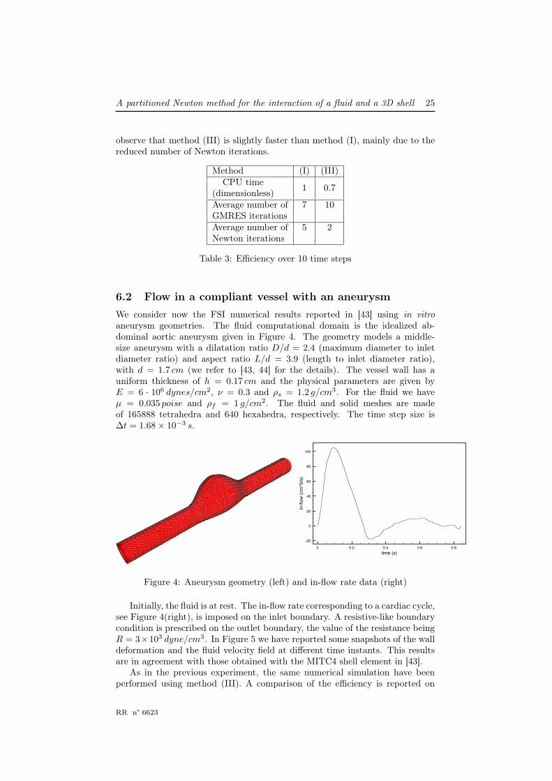
We consider now the FSI numerical results reported in [43] using in vitroaneurysm geometries. The fluid computational domain is the idealized ab-dominal aortic aneurysm given in Figure 4. The geometry models a middle-size aneurysm with a dilatation ratio D/d = 2.4 (maximum diameter to inletdiameter ratio) and aspect ratio L/d = 3.9 (length to inlet diameter ratio),with d = 1.7 cm (we refer to [43, 44] for the details). The vessel wall has auniform thickness of h = 0.17 cm and the physical parameters are given byE = 6 · 106 dynes/cm2, ν = 0.3 and ρs = 1.2 g/cm3. For the fluid we haveµ = 0.035 poise and ρf = 1 g/cm2. The fluid and solid meshes are madeof 165888 tetrahedra and 640 hexahedra, respectively. The time step size is∆t = 1.68× 10⁻³ s.
0 0.2 0.4 0.6 0.8
time (s)
-20
0
20
40
60
80
100
in-fl
ow
(cm
^3/s
)
Figure 4: Aneurysm geometry (left) and in-flow rate data (right)
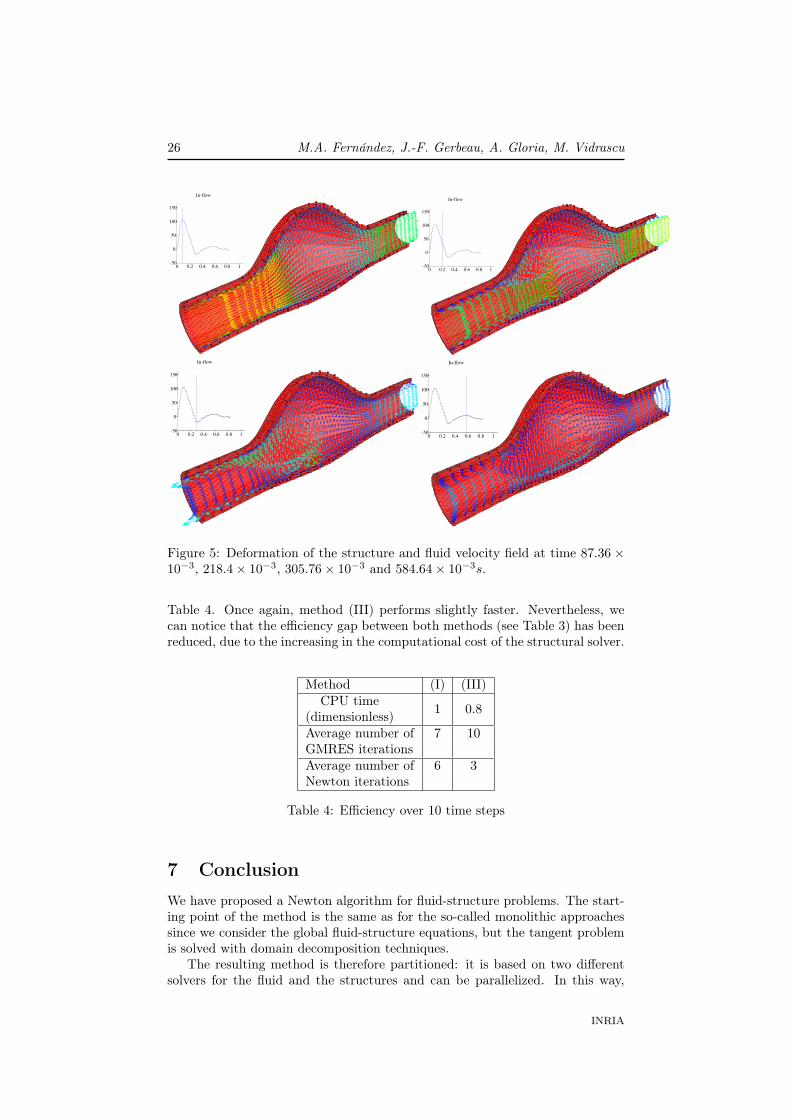
Initially, the fluid is at rest. The in-flow rate corresponding to a cardiac cycle,see Figure 4(right), is imposed on the inlet boundary. A resistive-like boundarycondition is prescribed on the outlet boundary, the value of the resistance beingR = 3×10³ dyne/cm3. In Figure 5 we have reported some snapshots of the walldeformation and the fluid velocity field at different time instants. This resultsare in agreement with those obtained with the MITC4 shell element in [43].
As in the previous experiment, the same numerical simulation have beenperformed using method (III). A comparison of the efficiency is reported on
RR n° 6623
26 M.A. Fernández, J.-F. Gerbeau, A. Gloria, M. Vidrascu
In-flow
0 0.2 0.4 0.6 0.8 1-50
0
50
100
150
In-flow
0 0.2 0.4 0.6 0.8 1-50
0
50
100
150
In-flow
0 0.2 0.4 0.6 0.8 1-50
0
50
100
150
In-flow
0 0.2 0.4 0.6 0.8 1-50
0
50
100
150
Figure 5: Deformation of the structure and fluid velocity field at time 87.36 ×10⁻³, 218.4× 10⁻³, 305.76× 10⁻³ and 584.64× 10⁻³s.
Table 4. Once again, method (III) performs slightly faster. Nevertheless, wecan notice that the efficiency gap between both methods (see Table 3) has beenreduced, due to the increasing in the computational cost of the structural solver.
Method (I) (III)CPU time
(dimensionless)1 0.8
Average number of 7 10GMRES iterationsAverage number of 6 3Newton iterations
Table 4: Efficiency over 10 time steps
7 Conclusion
We have proposed a Newton algorithm for fluid-structure problems. The start-ing point of the method is the same as for the so-called monolithic approachessince we consider the global fluid-structure equations, but the tangent problemis solved with domain decomposition techniques.
The resulting method is therefore partitioned: it is based on two differentsolvers for the fluid and the structures and can be parallelized. In this way,
INRIA

A partitioned Newton method for the interaction of a fluid and a 3D shell 27
the proposed approach overcomes one of the main drawbacks of the standardmonolithic schemes used in fluid-structure interaction.
As regards efficiency, a simplified complexity analysis showed that the pro-posed scheme is expected to reach optimal performance when the structure andfluid solvers are very expensive, provided that the global number of Newton iter-ations is of the same order. In spite of that, the numerical results reported in thispaper showed that the proposed approaches do not outperform some classicalpartitioned Newton procedures in which the domain decomposition frameworkis applied at the nonlinear level [26, 23, 14]. This information should be takeninto consideration by those interested in developing a monolothic fluid-structureinteraction solver.
References
[1] S. Badia, F. Nobile, and C. Vergara. Fluid-structure partitioned proceduresbased on Robin transmission conditions. J. Comp. Phys., 227:7027–7051,2008.
[2] K.J. Bathe and H. Zhang. Finite element developments for general fluidflows with structural interactions. Int. J. Num. Meth. Engng., 2004.
[3] J.T. Batina. Unsteady Euler airfoil solutions using unstructured dynamicmeshes. AIAA J., 28(8):1381–1388, 1990.
[4] Y. Bazilevs, V.M. Calo, T.J.R. Hughes, and Y. Zhang. Isogeometric fluid-structure interaction: Theory, algorithms, and computations. TechnicalReport 08-16, ICES, 2008.
[5] Y. Bazilevs, V.M. Calo, Y. Zhang, and T.J.R. Hughes. Isogeometric fluid-structure interaction analysis with applications to arterial blood flow. Com-put. Mech., 38:310–322, 2006.
[6] E. Burman and M.A. Fernández. Stabilized explicit coupling for fluid-structure interaction using Nitsche’s method. C. R. Math. Acad. Sci. Paris,345(8):467–472, 2007.
[7] D. Caillerie, A. Mourad, and Raoult A. Cell-to-muscle homogenization.Application to a constitutive law for the myocardium. Math. Model. Num.Anal., 37:681–698, 2003.
[8] P. Causin, J.-F. Gerbeau, and F. Nobile. Added-mass effect in the designof partitioned algorithms for fluid-structure problems. Comp. Meth. Appl.Mech. Engng., 194(42–44):4506–4527, 2005.
[9] D. Chapelle and K.J. Bathe. The Finite Element Analysis of Shells - Fun-damentals. Springer Verlag, 2003.
[10] D. Chapelle and A. Ferent. Modeling of the inclusion of a reinforcing sheetwithin a 3D medium. Math. Models Methods Appl. Sci., 13(4):573–595,2003.
RR n° 6623
28 M.A. Fernández, J.-F. Gerbeau, A. Gloria, M. Vidrascu
[11] D. Chapelle, A. Ferent, and K.J. Bathe. 3D-shell elements and their under-lying mathematical model. Math. Models Methods Appl. Sci., 14(1):105–142, 2004.
[12] D. Chapelle, A. Ferent, and P. Le Tallec. The treatment of "pinching lock-ing" in 3D-shell elements. M2AN Math. Model. Numer. Anal., 37(1):143–158, 2003.
[13] S. Deparis. Numerical Analysis of Axisymmetric Flows and Methods forFluid-Structure Interaction Arising in Blood Flow Simulation. PhD thesis,EPFL, Switzerland, 2004.
[14] S. Deparis, M. Discacciati, G. Fourestey, and A. Quarteroni. Fluid-structure algorithms based on Steklov-Poincaré operators. Comput. Meth-ods Appl. Mech. Engrg., 195(41-43):5797–5812, 2006.
[15] S. Deparis, M. Discacciati, and A. Quarteroni. A domain decompositionframework for fluid-structure interaction problems. In Proceedings of theThird International Conference on Computational Fluid Dynamics (IC-CFD3), 2004.
[16] W. Dettmer and D. Perić. A computational framework for fluid-structureinteraction: Finite element formulation and applications. Comp. Meth.Appl. Mech. Engrg., 195(41-43):5754–5779, 2006.
[17] J. Donéa, S. Giuliani, and J. P. Halleux. An arbitrary Lagrangian-Eulerianfinite element method for transient dynamic fluid-structure interactions.Comp. Meth. Appl. Mech. Engng., pages 689–723, 1982.
[18] C. Farhat, K. van der Zee, and Ph. Geuzaine. Provably second-order time-accurate loosely-coupled solution algorithms for transient nonlinear aeroe-lasticity. Comp. Meth. Appl. Mech. Engng., 195(17-18):1973–2001, 2006.
[19] M.A. Fernández, J.-F. Gerbeau, and C. Grandmont. A projection algorithmfor fluid-structure interaction problems with strong added-mass effect. C.R. Acad. Sci. Paris, Math., 342:279–284, 2006.
[20] M.A. Fernández, J.-F. Gerbeau, and C. Grandmont. A projection semi-implicit scheme for the coupling of an elastic structure with an incompress-ible fluid. Int. J. Num. Meth. Engng. in press, 2006.
[21] M.A. Fernández and M. Moubachir. An exact block-Newton algorithm forsolving fluid-structure interaction problems. C. R. Math. Acad. Sci. Paris,336(8):681–686, 2003.
[22] M.A. Fernández and M. Moubachir. An exact block-newton algorithmfor the solution of implicit time discretized coupled systems involved influid-structure interaction problems. In K.J. Bathe, editor, Second M.I.T.Conference on Computational Fluid and Solid Mechanics, pages 1337–1341.Elsevier, 2003.
[23] M.A. Fernández and M. Moubachir. A Newton method using exact Jaco-bians for solving fluid-structure coupling. Comp. & Struct., 83:127–142,2005.
INRIA
A partitioned Newton method for the interaction of a fluid and a 3D shell 29
[24] L. Formaggia, J.-F. Gerbeau, F. Nobile, and A. Quarteroni. On the cou-pling of 3D and 1D Navier-Stokes equations for flow problems in compliantvessels. Comp. Meth. Appl. Mech. Engrg., 191(6-7):561–582, 2001.
[25] Y.C. Fung, K. Fronek, and P. Patitucci. Pseudoelasticity of arteries andthe choice of its mathematical expression. Am. J. Physiol., 237:620–631,1979.
[26] J.-F. Gerbeau and M. Vidrascu. A quasi-Newton algorithm based on a re-duced model for fluid-structure interactions problems in blood flows. Math.Model. Num. Anal., 37(4):631–648, 2003.
[27] J.-F. Gerbeau, M. Vidrascu, and P. Frey. Fluid-structure interaction inblood flows on geometries based on medical imaging. Comp. & Struct.,83(2-3):155–165, 2005.
[28] M. Heil. An efficient solver for the fully coupled solution of large-displacement fluid-structure interaction problems. Comput. Methods Appl.Mech. Engrg., 193(1-2):1–23, 2004.
[29] A.H. Holzapfel, T.C. Gasser, and Ogden R.W. A new constitutive frame-work for arterial wall mechanics and a comparative study of material mod-els. J. Elasticity, 61:1–48, 2000.
[30] B. Hübner, E. Walhorn, and D. Dinkle. A monolithic approach to fluid-structure interaction using space-time finite elements. Comp. Meth. Appl.Mech. Engng., 193:2087–2104, 2004.
[31] U. Küttler and W.A. Wall. Fixed-point fluid-structure interaction solverswith dynamic relaxation. Comput. Mech., 2008. DOI 10.1007/s00466-008-0255-5.
[32] P. Le Tallec. Domain decomposition methods in computational mechanics.In Computational Mechanics Advances, Vol. 1, no.2, pages 123–217. NorthHolland, 1994.
[33] P. Le Tallec and J. Mouro. Fluid structure interaction with large structuraldisplacements. Comput. Meth. Appl. Mech. Engrg., 190:3039–3067, 2001.
[34] H.G. Matthies and J. Steindorf. Partitioned but strongly coupled iterationschemes for nonlinear fluid-structure interaction. Comp. & Struct., 80(27–30):1991–1999, 2002.
[35] H.G. Matthies and J. Steindorf. Partitioned strong coupling algorithms forfluid-structure interaction. Comp. & Struct., 81:805–812, 2003.
[36] D. P. Mok and W. A. Wall. Partitioned analysis schemes for the tran-sient interaction of incompressible flows and nonlinear flexible structures.In K. Schweizerhof W.A. Wall, K.U. Bletzinger, editor, Trends in compu-tational structural mechanics, Barcelona, 2001. CIMNE.
[37] D. P. Mok, W. A. Wall, and E. Ramm. Partitioned analysis approach forthe transient, coupled response of viscous fluids and flexible structures. InW. Wunderlich, editor, Proceedings of the European Conference on Com-putational Mechanics. ECCM’99, TU Munich, 1999.
RR n° 6623

30 M.A. Fernández, J.-F. Gerbeau, A. Gloria, M. Vidrascu
[38] D. P. Mok, W. A. Wall, and E. Ramm. Accelerated iterative substructuringschemes for instationary fluid-structure interaction. In K.J. Bathe, editor,Computational Fluid and Solid Mechanics, pages 1325–1328. Elsevier, 2001.
[39] F. Nobile. Numerical approximation of fluid-structure interaction problemswith application to haemodynamics. PhD thesis, EPFL, Switzerland, 2001.
[40] Christiaan H.G.A. van Oijen. Mechanics and design of fiber-reinforced vas-cular prostheses. PhD thesis, Technische Universiteit Eindhoven, 2003.
[41] S. Piperno, C. Farhat, and B. Larrouturou. Partitioned procedures for thetransient solution of coupled aeroelastic problems. Part I: Model problem,theory and two-dimensional application. Comp. Meth. Appl. Mech. Engrg.,124:79–112, 1995.
[42] S. Rugonyi and K.J. Bathe. On finite element analysis of fluid flows coupledwith structural interaction. CMES - Comp. Modeling Eng. Sci., 2(2):195–212, 2001.
[43] A.-V. Salsac, M.A. Fernández, J.M. Chomaz, and P. Le Tallec. Effects of theflexibility of the arterial wall on the wall shear stresses and wall tension inabdominal aortic aneurysms. In Bulletin of the American Physical Society,2005.
[44] A.-V. Salsac, S.R. Sparks, J.M. Chomaz, and J.C. Lasheras. Evolutionof the wall shear stresses during the progressive enlargement of symmetricabdominal aortic aneurysms. J. Fluid Mech., 550:19–51, 2006.
[45] T.E. Tezduyar. Finite element methods for fluid dynamics with movingboundaries and interfaces. Arch. Comput. Methods Engrg., 8:83–130, 2001.
[46] P.D. Thomas and C.K. Lombard. Geometric conservation law and its appli-cation to flow computations on moving grids. AIAA J., 17(10):1030–1037,1979.
[47] J. Vierendeels. Implicit coupling of partioned fluid-structure interactionsolvers using reduced order models. In M. Schäfer H.J. Bungartz, editor,Fluid-Structure interaction, Modelling, Simulation, Optimization, pages 1–18. Springer, 2006.
[48] H. Zhang, X. Zhang, S. Ji, G. Guo, Y. Ledezma, N. Elabbasi, and H. de-Cougny. Recent development of fluid-structure interaction capabilities inthe ADINA system. Computers & Structures, 81(8-11):1071–1085, 2003.
INRIA

Centre de recherche INRIA Paris – RocquencourtDomaine de Voluceau - Rocquencourt - BP 105 - 78153 Le Chesnay Cedex (France)
Centre de recherche INRIA Bordeaux – Sud Ouest : Domaine Universitaire - 351, cours de la Libération - 33405 Talence CedexCentre de recherche INRIA Grenoble – Rhône-Alpes : 655, avenue de l’Europe - 38334 Montbonnot Saint-Ismier
Centre de recherche INRIA Lille – Nord Europe : Parc Scientifique de la Haute Borne - 40, avenue Halley - 59650 Villeneuve d’AscqCentre de recherche INRIA Nancy – Grand Est : LORIA, Technopôle de Nancy-Brabois - Campus scientifique
615, rue du Jardin Botanique - BP 101 - 54602 Villers-lès-Nancy CedexCentre de recherche INRIA Rennes – Bretagne Atlantique : IRISA, Campus universitaire de Beaulieu - 35042 Rennes Cedex
Centre de recherche INRIA Saclay – Île-de-France : Parc Orsay Université - ZAC des Vignes : 4, rue Jacques Monod - 91893 Orsay CedexCentre de recherche INRIA Sophia Antipolis – Méditerranée : 2004, route des Lucioles - BP 93 - 06902 Sophia Antipolis Cedex
ÉditeurINRIA - Domaine de Voluceau - Rocquencourt, BP 105 - 78153 Le Chesnay Cedex (France)
http://www.inria.fr
ISSN 0249-6399

![Partitioned Fluid-Structure Interaction Techniques Applied ... · FEM bearing model [3], from which only the degrees of freedom of the nodes placed on the internal 15 bearing surface](https://img.pdfslide.net/doc/110x75/602213974a61943665711eca/partitioned-fluid-structure-interaction-techniques-applied-fem-bearing-model.jpg)