Embed Size (px)
Citation preview
Vision Research xxx (2015) xxx–xxx
Contents lists available at ScienceDirect
Vision Research
journal homepage: www.elsevier .com/locate /v isres
A perceptual space of local image statistics
http://dx.doi.org/10.1016/j.visres.2015.05.0180042-6989/� 2015 Elsevier Ltd. All rights reserved.
⇑ Corresponding author. Fax: +212 746 8050.E-mail address: [email protected] (J.D. Victor).
Please cite this article in press as: Victor, J. D., et al. A perceptual space of local image statistics. Vision Research (2015), http://dx.doi.org/1j.visres.2015.05.018
Jonathan D. Victor ⇑, Daniel J. Thengone, Syed M. Rizvi, Mary M. ConteBrain and Mind Research Institute, Weill Cornell Medical College, 1300 York Avenue, New York, NY 10065, United States
a r t i c l e i n f o a b s t r a c t
Article history:Received 29 October 2014Received in revised form 28 May 2015Accepted 30 May 2015Available online xxxx
Keywords:Local featuresVisual texturesMetamersMultipoint correlationsIntermediate vision
Local image statistics are important for visual analysis of textures, surfaces, and form. There are manykinds of local statistics, including those that capture luminance distributions, spatial contrast, orientedsegments, and corners. While sensitivity to each of these kinds of statistics have been well-studied, muchless is known about visual processing when multiple kinds of statistics are relevant, in large part becausethe dimensionality of the problem is high and different kinds of statistics interact. To approach this prob-lem, we focused on binary images on a square lattice – a reduced set of stimuli which nevertheless tapsmany kinds of local statistics. In this 10-parameter space, we determined psychophysical thresholds toeach kind of statistic (16 observers) and all of their pairwise combinations (4 observers). Sensitivitiesand isodiscrimination contours were consistent across observers. Isodiscrimination contours were ellip-tical, implying a quadratic interaction rule, which in turn determined ellipsoidal isodiscrimination sur-faces in the full 10-dimensional space, and made predictions for sensitivities to complex combinationsof statistics. These predictions, including the prediction of a combination of statistics that was metamericto random, were verified experimentally. Finally, check size had only a mild effect on sensitivities overthe range from 2.8 to 14 min, but sensitivities to second- and higher-order statistics was substantiallylower at 1.4 min. In sum, local image statistics form a perceptual space that is highly stereotyped acrossobservers, in which different kinds of statistics interact according to simple rules.
� 2015 Elsevier Ltd. All rights reserved.
1. Introduction
The analysis of image statistics underlies many key componentsof intermediate visual processing, including not only visual texture,but also visual characterization of surfaces and segmentation ofimages into objects. Although each of these tasks might at firstseem deterministic, each is fundamentally statistical. For example,identification of surface materials (such as wood, grass, or hair) isnot carried out by matching the image to a stored sample, butrather, by their image statistics, such as the range of contrastsand colors and the distribution of oriented contours at differentscales (Karklin & Lewicki, 2009). Segmentation of an image is a sta-tistical task as well, because it is fundamentally ambiguous: multi-ple scene interpretations are consistent with a single image, andimage statistics play a key role in assessing which one is chosenas the most plausible. For example, contours due to a shadow orchange in illumination are not typically coincident with a changein material properties, while real object boundaries typically havesuch changes, and hence, changes in image statistics.
Thus, understanding the processing of image statistics hasbroad importance as part of a foundation for understanding many
aspects of intermediate visual processing. Visual textures, the focushere, present image statistics in their purest form.
While natural textures are characterized by many kinds of sta-tistical features, systematic approaches to studying visual texture(with few exceptions (Motoyoshi & Kingdom, 2007; Saarela &Landy, 2012; Victor, Chubb, & Conte, 2005)) usually explore justone kind of feature, such as luminance distributions (Chubb,Econopouly, & Landy, 1994; Chubb, Landy, & Econopouly, 2004),color (Li & Lennie, 1997), orientation (Landy & Oruc, 2002;Wolfson & Landy, 1995, 1998), or curvature (Ben-Shahar &Zucker, 2004). There are two main reasons for this. One is the highdimensionality of the problem: if all kinds of statistical featureswere explored, the number of parameters (i.e., the number of dif-ferent image statistics) would be impractically large. The other isthat image statistics exhibit a high degree of interdependency.Edges cannot exist without local changes in luminance, and cor-ners cannot exist without edges at multiple orientations, so thesestatistics cannot be considered to be independent attributes.Here, we attempt to address both issues, by constructing a texturespace of large but manageable dimension (10), whose coordinatestake into account the interactions implied by geometry. The datashow that once these steps are taken, the perceptual interactionsof image statistics obey simple rules that (a) are highly consistentacross subjects, (b) accurately predict sensitivity to complex
0.1016/
2 J.D. Victor et al. / Vision Research xxx (2015) xxx–xxx
combinations of image statistics, and (c) are approximately pre-served across a range of spatial scales.
To overcome the problem of high dimensionality (specifically,that an image statistic can be defined from the joint probabilitiesof any set of gray levels at any configuration of nearby points),we restricted consideration to black-and-white images on acheckerboard. By restricting the analysis to a single scale and onlytwo luminance levels, we can then consider all possible localimages statistics – i.e., the probabilities of all configurations ofblack and white checks within a 2 � 2 neighborhood. This set ofimage statistics has 10 free parameters (summarized here inMethods; detailed in (Victor & Conte, 2012)). It encompasses notonly the intuitively-important features of luminance, contrast,edge, and corner, but also, its four-point correlations are indepen-dently informative for natural images (Tkacik et al., 2010). Thus,although it is a reduced space, it has image statistics of many dif-ferent types and levels of complexity.
To overcome the second hurdle, the interdependency of differ-ent kinds of stimulus features, we used a ‘‘maximum-entropy’’approach. That is, we specify stimuli by the prevalence of one ormore elementary features, and then synthesize an ensemble ofimages that meet these specifications but are otherwise as randomas possible. This limits the interdependence of features to what isimplied by geometry, so that observed interactions at the level ofneural or perceptual responses can be more readily interpreted.
1.1. Texture space and color space: their geometry and its implications
The above considerations lead to the construction of a ‘‘texturespace’’, in which each point corresponds to a specific combinationof image statistics that together specify luminance distributions andthe prevalence of edges and corners at different orientations (Victor& Conte, 2012). The experiments presented here determine the per-ceptual distances in this space, focusing on the region near its origin.
The analogy with trichromatic color space provides a helpfulgeometrical framework. In both color space and texture space,points represent stimuli and the origin represents the neutral point(in color space, a white light; here, the random texture). The pre-sent experiments, which consist of measuring thresholds for per-ceiving that a texture is not random, correspond to measuringthresholds to changes in color and intensity near the white point.In both spaces, a line segment space represents mixtures. In colorspace, the points on a line segment are the colors that can be cre-ated by mixing the lights that correspond to the endpoints. In thespace of local image statistics, the points on a line segment are thetextures that can be created by mixing the textures that corre-spond to the endpoint. In color space, mixtures are created byphysical mixing of lights; here, mixtures are created at the levelof statistics: at the level of the frequency of each way that a2 � 2 block can be colored with black and white checks (asdescribed in (Victor & Conte, 2012). In color space and in texturespace, a ray emanating from the origin corresponds to a set of stim-uli that are progressively more saturated. Thus, determining thepoint along this ray that is first discriminable from the origin is away of quantifying sensitivity to the combination of features rep-resented by the direction of the ray. By determining the thresholdsfor rays that emanate from the origin in many directions, one canmap out the ‘‘isodiscrimination surface,’’ which summarizes theperceptual sensitivities in the neighborhood of the origin. In thecase of color space, the isodiscrimination surfaces are approxi-mately ellipsoids (the ‘‘Macadam ellipses’’ (Macadam, 1942)), andbelow we find that this holds in texture space as well.
The notion of navigating the space by moving along a straightline trajectory brings up an important mathematical distinctionbetween the geometries of the two spaces. In color space, movingalong a line is straightforward: it corresponds to increasing or
Please cite this article in press as: Victor, J. D., et al. A perceptual space ofj.visres.2015.05.018
decreasing the intensity of a light. For textures, this is not the case.For example, increasing the number of edges may also increase thenumber of intersections, and the proportionality between cornersand intersections is typically nonlinear. These nonlinear dependen-cies underlie the maximum entropy approach (Victor & Conte,2012) for navigating the space: a direction in the space corre-sponds to a specified coordinate, and movement along this direc-tion may take a curved path to minimize the introduction offurther structure. That is, the maximum-entropy approach yieldsa locally flattened coordinate system. Here, since we are studyingdiscrimination thresholds, we work in these local coordinates,and ignore the impact of global curvature.
Color space and texture space have other important differences,and these allow us to interpret the sensitivity measurements in away that has no immediate analogy in color space. The differencesgo beyond the difference in dimensionality or global curvature,and trace back to a fundamental difference in the way that the coor-dinate systems are defined. For color space, the origin of the coordi-nate system – the white point – is defined subjectively. For imagestatistics, the origin of the texture space has an a priori mathematicaldefinition: it is the texture in which each check is randomly andindependently assigned to black or white. A similar distinctionapplies to the axes: for color space, axes are defined empiricallybased on cone excitations (MacLeod & Boynton, 1979) or combina-tions motivated by physiological and psychophysical measurements(Derrington, Krauskopf, & Lennie, 1984); for image statistics, axesare defined a priori mathematically, in terms of correlations.
The kind of geometry that applies to the two spaces is also differ-ent (Zaidi et al., 2013). In color space, any of several coordinate sys-tems (Derrington, Krauskopf, & Lennie, 1984; MacLeod & Boynton,1979; Wyszecki & Stiles, 1967), each based on its own set of empir-ical observations, are equally valid descriptions of the space.Changing from one set of axes to another is a general linear trans-formation, which means that distances and angles computed fromthe coordinates in one system (via the Pythagorean rule anddot-products) need not match values computed with another. Inthe space of local image statistics, the coordinates are defined bymathematical considerations. This means that there is a standarddefinition of distance, and a ‘‘sphere’’ is a well-defined term: it isthe locus of points that are at an equal distance from its center.
Because of the mathematics underlying the texture-space coor-dinates, spheres centered at the origin have another interpretation.Specifically, spheres are the isodiscrimination surfaces for an idealobserver ((Victor & Conte, 2012), Appendix B), i.e., an observerwho is able to make full use of all image statistics. Of course we donot anticipate that human performance will resemble this. Rather,we expect that human observers will be selective, and make use ofsome image statistics more efficiently than others. This will distortthe human isodiscrimination surface away from a spherical shape.For example, if sensitivity is reduced along one axis, then the isodis-crimination surface will become elongated in that direction, into anellipsoid. If sensitivity is different for positive vs. negative changes ina coordinate, the surface will be asymmetrically distorted (i.e., it willbecome egg-shaped). If cues along different coordinates are notcombined, the shape of the isodiscrimination surface will becomesquared-off. But as the results show, only the first kind of distortionis prominent, and this enables a concise, predictively accurate modelfor sensitivity to complex combinations of image statistics.
2. Methods
2.1. The stimulus space
The goal of these experiments is to determine visual sensitivityto local image statistics, individually and in combination. To do
local image statistics. Vision Research (2015), http://dx.doi.org/10.1016/
J.D. Victor et al. / Vision Research xxx (2015) xxx–xxx 3
this, we use stimuli in which one or more local statistics are spec-ified, and all other aspects of the image are as random as possible,subject to these specifications. We consider only binary(black-and-white) images; for such images, there are 16 ways inwhich a 2 � 2 block can be colored ð16 ¼ 22�2Þ. These 16 potentialdegrees of freedom are reduced to 10, because the 2 � 2 blocksmust match where they overlap. Here we describe 10 natural coor-dinates that capture these degrees of freedom, and how they arecombined to generate the stimuli used in the experiments. For acomplete description of the space and details of the algorithmsto construct the stimuli within it, see (Victor & Conte, 2012).
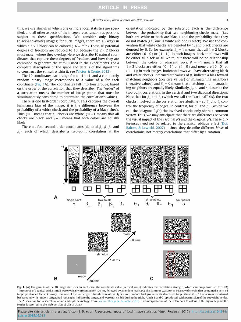
The 10 coordinates each range from �1 to 1, and a completelyrandom binary image corresponds to a value of 0 for eachcoordinate (Fig. 1A). The coordinates fall into four groups, basedon the order of the correlation that they describe. (The ‘‘order’’ ofa correlation means the number of image points that must besimultaneously considered to determine the correlation’s value.)
There is one first-order coordinate, c. This captures the overallluminance bias of the image: it is the difference between theprobability of a white check and the probability of a black check.Thus c = 1 means that all checks are white, c = �1 means that allchecks are black, and c = 0 means that both colors are equallylikely.
There are four second-order coordinates (denoted b , bj, bn, andb=), each of which describe a two-point correlation at the
Fig. 1. (A) The gamuts of the 10 image statistics. In each case, the coordinate value (veTimecourse of a typical trial. Stimuli were typically presented for 120 ms, followed by a ratarget positioned 8 checks away from one of the four edges. Stimuli were of two types:background with random target. Red rectangles indicate the target, and were not visible dThe Association for Research in Vision and Ophthalmology, from (Victor, Thengone, & Coreader is referred to the web version of this article.)
Please cite this article in press as: Victor, J. D., et al. A perceptual space ofj.visres.2015.05.018
orientation indicated by the subscript. Each is the differencebetween the probability that two neighboring checks match (i.e.,both are white or both are black), and the probability that theydo not match (i.e., one is white and one is black). We use the con-vention that white checks are denoted by 1, and black checks aredenoted by 0. So for example, b ¼ 1 means that all 1 � 2 blocksare either ð0 0 Þ or ð1 1 Þ; in such images, horizontal rows willbe either all black or all white, but there will be no relationshipbetween the colors of adjacent rows. b ¼ �1 means that all1 � 2 blocks are either ð0 1 Þ or ð1 0 Þ and none are ð0 0 Þ orð1 1 Þ; in such images, horizontal rows will have alternating blackand white checks. Intermediate values of b indicate a bias towardmatching neighbors (positive values) or mismatching neighbors(negative values), and b ¼ 0 means that matching and mismatch-ing neighbors are equally likely. Similarly, bj, bn, and b= describe thetwo-point correlations in the vertical and two diagonal directions.Note that for b and bj (which we call the ‘‘cardinal’’ b’s), the twochecks involved in the correlation are abutting – so b and bj con-trol the frequency of edges. In contrast, for bn, and b=, (which wecall the ‘‘diagonal’’ b’s) the involved checks only share a commonvertex. Thus, we may anticipate that there are differences betweenthe visual impact of the cardinal b’s and the diagonal b’s. These dif-ferences need not be related to the classical oblique effect (Doi,Balcan, & Lewicki, 2007) – since they describe different kinds ofcorrelations, not merely correlations that differ by a rotation.
rtical scale) indicates the correlation strength, which can range from �1 to 1. (B)ndom mask. (C) The stimulus was a 64 � 64 array of checks that contained a 16 � 64top, random background with structured target (here, hy ¼ 1), or bottom, structureduring the trials. Panels B and C reproduced, with permission of the copyright holder,nte, 2013). (For interpretation of the references to colour in this figure legend, the
local image statistics. Vision Research (2015), http://dx.doi.org/10.1016/
4 J.D. Victor et al. / Vision Research xxx (2015) xxx–xxx
Next, there are four third-order coordinates, hy, hx, hp, and hq.Each quantifies a three-point correlation within an L-shapedregion, by comparing the probability that the region contains aneven number of white checks, vs. an odd number of white checks.A value of +1 means that only an odd number of white checks (oneor three) are present. For example, hx ¼ 1 means that only the con-
figurations 11 1
� �, 1
0 0
� �, 0
1 0
� �or 0
0 1
� �are present;
this will lead to images with prominent white triangular-shapedregions pointing downward and to the left. hx ¼ �1 means that
only the complementary configurations 00 0
� �, 0
1 1
� �,
00 1
� �or 1
1 0
� �are present; these images have prominent
black triangular-shaped regions.The final coordinate, a, quantifies the four-point correlation
among the checks in a 2 � 2 block: a = 1 means that an even num-ber of them are white, and a = �1 means that an odd number arewhite. This is the same image statistic that has been the subjectof much previous work (Julesz, Gilbert, & Victor, 1978; Victor,Chubb, & Conte, 2005; Victor & Conte, 1989, 1991, 1996, 2004).
Together, the ten coordinates fc; b ; bj; bn; b=; hy; hx; hp; hq;ag fullyspecify the distribution of colorings in 2 � 2 blocks.
2.2. Stimuli
All experiments used the texture segmentation paradigm(Fig. 1B and C) first developed by Chubb and coworkers for thestudy of textures in which each check’s luminance is indepen-dently chosen from the same distribution (Chubb, Landy, &Econopouly, 2004), and later used for correlated textures (Victor,Chubb, & Conte, 2005; Victor & Conte, 2012; Victor, Thengone, &Conte, 2013). The psychophysical paradigm and stimulus layoutis taken from the latter studies, and is summarized here.
The basic stimulus (Fig. 1B and C) consisted of a 64 � 64 array ofchecks, which contained a 16 � 64 rectangular target, positioned 8checks away from one of the four edges of the array. The target wasdistinguished from the remainder of the array by its statistics, i.e.,by one or more values of fc; b ; bj; bn; b=; hy; hx; hp; hq;ag. The sub-ject’s task was to identify the location of the target via key-presson a response box.
To ensure that the subject identified the target by segmenting itfrom the background rather than, for example, by identifying a tex-ture gradient (Wolfson & Landy, 1998), two types of stimuli wereconstructed (Fig. 1C): (1) a random background array, with a targetthat had a nonzero value of one or more image statistics, and (2) abackground array in which the image statistics had a nonzerovalue, with a target that was random. Our rationale (both hereand in previous studies mentioned above using this design) forrequiring segmentation rather than just gradient detection wasto reduce intra- and inter-subject variability due to strategy choice.These two types of stimuli were randomly interleaved, and ouranalyses are based on the pooled responses.
There were two kinds of experiments. In the first, we measuredsensitivity to individual image statistics and their pairwise combi-nations. These measurements were used to construct a phe-nomenological model, and we used the model to predictsensitivities to combinations of multiple image statistics. In thesecond kind of experiment, we measured sensitivities to thesecombinations.
For the first kind of experiment, each session examined a singleplane of the stimulus space (i.e., a set of images in which two of thecoordinates fc; b ; bj; bn; b=; hy; hx; hp; hq;ag were given specific non-zero values.) Since there are 10 coordinates, there are45 = 10 � 9/2 different planes, one corresponding to each
Please cite this article in press as: Victor, J. D., et al. A perceptual space ofj.visres.2015.05.018
coordinate pair. However, many of these planes differ only by a90� rotation or mirror reflection. Pilot studies and previous work(Victor, Thengone, & Conte, 2013) showed that visual sensitivitieswere not affected by these transformations, so we focused on a15-plane subset (the ones shown in Fig. 4) that included all combi-nations, once these symmetries are taken into account.
Each of these 15 planes was explored in a radial fashion, in mostcases by choosing points at several distances from the origin along8 rays. For the four rays along the coordinate axes (the positive andnegative directions of the two axes in the plane), we used fiveequally-spaced values, with the maximal values chosen based onpilot experiments to ensure that performance would span therange from floor to ceiling: ±0.25 for c, ± 0.45 for the cardinal b’s,±0.75 for the diagonal b’s, ±1.0 for the h’s, and ±0.85 for a. The otherfour rays pointed into each of the four quadrants, with maximalvalues chosen in approximate proportion to the above maximumvalues. These rays were sampled at two points: the maximal point,and a point in the same direction at a relative distance of 0.7 fromthe origin. In two of the planes ðc; hyÞ and ðhy;aÞ, we used a minormodification for consistency with an earlier pilot dataset, in whichthere were two rays pointing into each quadrant, and all 12 rays (4along the axes, and 8 oblique) were sampled at threeequally-spaced points. After assigning the in-plane coordinates asjust described, the 8 unspecified coordinates were determined(see (Victor & Conte, 2012) Table 2) by first, setting all values oflower-order coordinates to zero, and then, setting the remainingcoordinates to values that maximized the entropy of the resultingimages. Details on construction of these stimuli are provided in(Victor & Conte, 2012).
The second kind of experiment measured sensitivity to combi-nations of multiple image statistics. We considered 12 such combi-nations, each corresponding to a vector ~c (specified below) in the10-coordinate space. There were four kinds of sessions, each ofwhich focused on 3 of these ‘‘out-of-sample’’ directions, in twoopposite rays (i.e., þ~c and �~c). The four subjects who participatedin these experiments included two subjects who also participatedin the first set of experiments 6 months to 2 years previously(MC and DT), and two who had not (SR and KP). Each session there-fore also included stimuli along two of the coordinate axes (in pos-itive and negative directions, as described above); for MC and DT,this served as a check for a change in sensitivity over time, forthe others, it served as a measure of overall sensitivity to theon-axis stimuli to scale the model predictions.
The 12 out-of-sample directions were chosen to explore (i) therange of predicted sensitivities, (ii) the combinations of statisticstypically present in natural images, and (iii) the combinations thatdetermine the topological properties of a texture. For (i), we madeuse of the finding that the in-plane measurements suggested aquadratic perceptual metric, which can be captured in a symmetricmatrix (see below). The eigenvectors corresponding to the largestand smallest eigenvalues of this matrix are thus the predicteddirections of maximal and minimal sensitivities. Since there are10 dimensions, there are 10 eigenvectors in all, covering the rangeof predicted sensitivities (which, as shown below, included sensi-tivities predicted to be both above and below the range of thein-plane measurements). Three of these 10 eigenvectors were nottested, since they were included in the stimuli used to build themodel (one is in the ðb ; bjÞ-plane and two are in planes spannedby the h’s; see ‘‘Eigenvector classes’’ below), The remaining 7out-of-sample eigenvectors (listed in Table 3), which includedthe largest of the ten eigenvalues (sym1) and the smallest (hvi2),constituted the first 7 out-of-sample test directions ~c. Note thatsince these are the eigenvectors of a symmetric matrix, they arenecessarily orthogonal – and thus, probe different directions inthe perceptual space.
local image statistics. Vision Research (2015), http://dx.doi.org/10.1016/
J.D. Victor et al. / Vision Research xxx (2015) xxx–xxx 5
For the two subjects that participated in both kinds of experi-ments, we used the eigenvectors calculated from their sensitivitiesin the 15 coordinate planes. For the two naïve subjects, we usedthe eigenvectors calculated from the average of the four subjectswho participated in the 15-plane experiments (which were in goodagreement, see Fig. 5 and Table 3). These choices also satisfied cri-terion (ii), as the predicted directions of maximal and minimal sen-sitivity correspond closely to axes of greatest and least variation innatural images (Hermundstad et al., 2014). Note that the specificdirections were determined from experimental data, but the direc-tions themselves did not correspond to any of the data used to fitthe model.
To satisfy criterion (iii), i.e., to sample the combinations thatdetermine the topological properties of a texture, we made useof the Minkowski image functionals (Michielsen & De Raedt,2001), a series of measures that can be applied to images to extracttheir topological features. For binary images, there are three cardi-nal functionals, typically denoted A, U, and v. Considering theimages to represent material (with the black checks representingsubstance, and the white checks representing empty space), thethree functionals have simple meanings: A is density (amount ofsubstance per unit area), U is perimeter length (amount of bound-ary per unit area), and v is porosity (number of holes per unit area).The first two of these functionals correspond to axes or planes inour coordinate system: A ¼ ð1� cÞ=2 and U ¼ 1� ðb� þ bjÞ=2, andtherefore would not provide out-of-sample tests. So we focusedon v, which, other than an additive offset, is a linear combinationof multiple coordinates. This choice is also motivated by recentfindings that demonstrate human sensitivity to this imageattribute(Barbosa, Bubna-Litic, & Maddess, 2013). The precise rela-tionship of v to the coordinates depends on how one defines con-nectivity on the checkerboard lattice: 4-connected (i.e., thematerial is contiguous across two checks that share a commonside) vs. 8-connected (i.e., the material is contiguous across twochecks that share a common side or a common vertex). The rela-tionship can be obtained by transforming standard formulae (Eq.(5) of (Michielsen & De Raedt, 2001)) into our coordinates (see(Barbosa, Bubna-Litic, & Maddess, 2013) Appendices A and B fora related calculation):
v½4� � 116¼ 1
16ð�4c� 2b� � 2bj þ b= þ bn þ hy þ hx þ hp þ hq þ aÞ
ð1Þ
and
v½8� þ 116¼ 1
16ð�4cþ 2b� þ 2bj � b= � bn þ hy þ hx þ hp þ hq � aÞ:
ð2Þ
We therefore used these directions (the right hand sides of Eqs.(1) and (2) as out-of-sample test directions~c, as well as their sumsand differences:
v½4� þ v½8� ¼ 18ð�4cþ hy þ hx þ hp þ hqÞ; ð3Þ
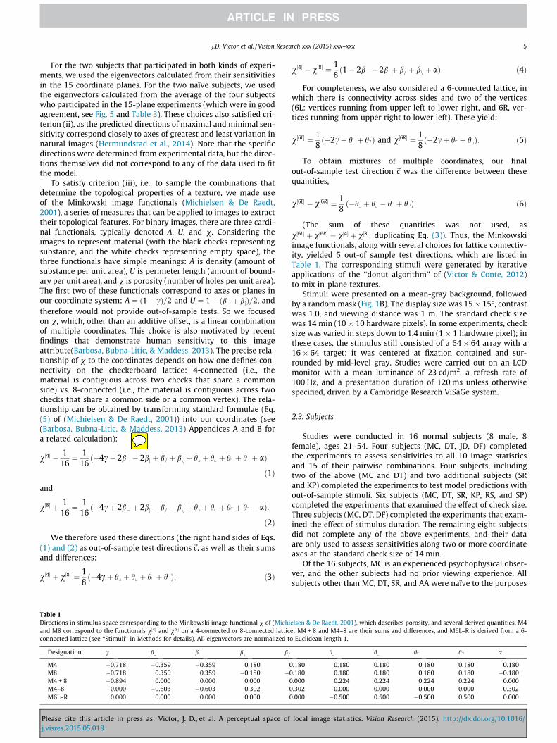
Table 1Directions in stimulus space corresponding to the Minkowski image functional v of (Michiand M8 correspond to the functionals v½4� and v½8� on a 4-connected or 8-connected latticconnected lattice (see ‘‘Stimuli’’ in Methods for details). All eigenvectors are normalized t
Designation c b bj bn b=
M4 �0.718 �0.359 �0.359 0.180 0M8 �0.718 0.359 0.359 �0.180 �0M4 + 8 �0.894 0.000 0.000 0.000 0M4–8 0.000 �0.603 �0.603 0.302 0M6L–R 0.000 0.000 0.000 0.000 0
Please cite this article in press as: Victor, J. D., et al. A perceptual space ofj.visres.2015.05.018
v½4� � v½8� ¼ 18ð1� 2b� � 2bj þ b= þ bn þ aÞ: ð4Þ
For completeness, we also considered a 6-connected lattice, inwhich there is connectivity across sides and two of the vertices(6L: vertices running from upper left to lower right, and 6R, ver-tices running from upper right to lower left). These yield:
v½6L� ¼ 18ð�2cþ hx þ hqÞ and v½6R� ¼ 1
8ð�2cþ hp þ hyÞ: ð5Þ
To obtain mixtures of multiple coordinates, our finalout-of-sample test direction ~c was the difference between thesequantities,
v½6L� � v½6R� ¼ 18ð�hy þ hx � hp þ hqÞ: ð6Þ
(The sum of these quantities was not used, asv½6L� þ v½6R� ¼ v½4� þ v½8�, duplicating Eq. (3)). Thus, the Minkowskiimage functionals, along with several choices for lattice connectiv-ity, yielded 5 out-of sample test directions, which are listed inTable 1. The corresponding stimuli were generated by iterativeapplications of the ‘‘donut algorithm’’ of (Victor & Conte, 2012)to mix in-plane textures.
Stimuli were presented on a mean-gray background, followedby a random mask (Fig. 1B). The display size was 15 � 15�, contrastwas 1.0, and viewing distance was 1 m. The standard check sizewas 14 min (10 � 10 hardware pixels). In some experiments, checksize was varied in steps down to 1.4 min (1 � 1 hardware pixel); inthese cases, the stimulus still consisted of a 64 � 64 array with a16 � 64 target; it was centered at fixation contained and sur-rounded by mid-level gray. Studies were carried out on an LCDmonitor with a mean luminance of 23 cd/m2, a refresh rate of100 Hz, and a presentation duration of 120 ms unless otherwisespecified, driven by a Cambridge Research ViSaGe system.
2.3. Subjects
Studies were conducted in 16 normal subjects (8 male, 8female), ages 21–54. Four subjects (MC, DT, JD, DF) completedthe experiments to assess sensitivities to all 10 image statisticsand 15 of their pairwise combinations. Four subjects, includingtwo of the above (MC and DT) and two additional subjects (SRand KP) completed the experiments to test model predictions without-of-sample stimuli. Six subjects (MC, DT, SR, KP, RS, and SP)completed the experiments that examined the effect of check size.Three subjects (MC, DT, DF) completed the experiments that exam-ined the effect of stimulus duration. The remaining eight subjectsdid not complete any of the above experiments, and their dataare only used to assess sensitivities along two or more coordinateaxes at the standard check size of 14 min.
Of the 16 subjects, MC is an experienced psychophysical obser-ver, and the other subjects had no prior viewing experience. Allsubjects other than MC, DT, SR, and AA were naïve to the purposes
elsen & De Raedt, 2001), which describes porosity, and several derived quantities. M4e; M4 + 8 and M4–8 are their sums and differences, and M6L–R is derived from a 6-o Euclidean length 1.
hy hx hp hq a
.180 0.180 0.180 0.180 0.180 0.180
.180 0.180 0.180 0.180 0.180 �0.180
.000 0.224 0.224 0.224 0.224 0.000
.302 0.000 0.000 0.000 0.000 0.302
.000 �0.500 0.500 �0.500 0.500 0.000
local image statistics. Vision Research (2015), http://dx.doi.org/10.1016/
6 J.D. Victor et al. / Vision Research xxx (2015) xxx–xxx
of the experiment. All subjects had visual acuities (corrected if nec-essary) of 20/20 or better.
This work was carried out in accordance with the Code of Ethicsof the World Medical Association (Declaration of Helsinki), andwith the approval of the Institutional Review Board of WeillCornell, and with the consents of the individual subjects.
2.4. Procedure
Subjects were asked to identify the position of the target, in afour-alternative forced choice (4-AFC) texture segregation task(Fig. 1B and C). They were informed that the target was equallylikely to appear in any of four locations (top, right, bottom, left),and were shown examples of stimuli of both types: target struc-tured/background random and target random/background struc-tured. They were asked to maintain central fixation, rather thanto attempt to scan the stimulus. Auditory feedback for incorrectresponses was given during training trials. After performance sta-bilized (approx. 2 h for a new subject), blocks of trials (with trialspresented in randomized order) were presented. Block order wascounterbalanced across subjects. Feedback was not given duringdata collection to minimize the likelihood of learning over thecourse of the experiment, as collection of complete datasets occu-pied approximately a year (see below). Thresholds for conditionsthat were tested at the beginning and end of the testing periodwere in good agreement.
Experiments were organized into several kinds of blocks. In theblocks used to probe sensitivity in coordinate planes, stimuli wereplaced along the positive and negative directions on each of twoaxes (4 directions, 5 strengths), and in four oblique directions inthe plane that these axes determined, at 2 strengths, with the latterrepeated twice, for a total of 36 = 4 � 5 + 4 � 2 � 2 stimulus speci-fications. This design was used for all coordinate planes except forðc;aÞ and ðhy;aÞ; in this case, we tested the four directions alongthe two axes and 8 oblique directions, each at 3 strengths, alsofor a total of 36 = 4 � 3 + 8 � 3 stimulus specifications. In theblocks used to test sensitivity to complex mixtures, we tested 10directions, each at 4 strengths (40 = 10 � 4 stimulus specifica-tions). Each stimulus specification was used eight times per block:once in each of four target locations, and in two configurations:target structured/background random and target random/back-ground structured (Fig. 1C). This resulted in 288 = 8 � 36 to320 = 8 � 40 trials per block. We collected 8 blocks per subject inthe check size experiments at each of 4 check sizes(9216 = 288 � 4 � 8 trials). For the other experiments, we collected15 blocks per subject per condition (4320 = 288 � 15 to4800 = 320 � 15 trials). This yielded 64–240 responses per coordi-nate in the stimulus space. A complete set of measurements of sen-sitivities along all axes and in each of the 15 coordinate planesrequired 64800 = 15 � 4320 trials per subject, and was carriedout over approximately 1 year.
2.5. Analysis
2.5.1. Determination of thresholds from psychophysical dataThe first step in data analysis consisted of determining thresh-
olds in each tested plane (i.e., along each ray emanating from theorigin). We adapted the procedure of Victor, Chubb, & Conte(2005) and Victor, Thengone, & Conte (2013), as summarized here.Along each ray r, we fit measured values of the fraction correct (FC)fit to Weibull functions via maximum likelihood:
FCðxÞ ¼ 14þ 3
4ð1� 2�ðx=arÞbr Þ; ð7Þ
where x is the distance from the origin, ar is the fitted threshold(i.e., the value of x at which FC = 0.625, halfway between chance,
Please cite this article in press as: Victor, J. D., et al. A perceptual space ofj.visres.2015.05.018
0.25, and perfect, 1.0), and br is the Weibull shape parameter. Thedistance x is determined in the ordinary Euclidean fashion: on thecoordinate axes, it is the absolute value of the coordinate; on the
oblique rays, it is calculated as x ¼ffiffiffiffiffiffiffiffiffiffiffiffiffiffiffic2
y þ c2z
q, where cy and cz are
the values of the two coordinates, each drawn fromfc; b ;bj;bn; b=; hy; hx; hp; hq;ag that specify the stimulus. In nearlyall cases, the exponent br had 95% confidence limits that includedthe range 2.2 to 2.7. Since our focus was on thresholds, we thereforerefit the data from all rays within a coordinate plane by a set ofWeibull functions constrained to share a common exponent b, butwith the threshold parameter ar allowed to vary across rays. 95%confidence limits for ar were determined via 1000-sample boot-straps. Sensitivity is defined as 1/threshold, with correspondingconfidence limits. On some rays, performance was close to chance,and the upper confidence limit of these bootstraps was large (e.g.,>105); in these cases, sensitivity was taken to be zero.
Averages across subjects of sensitivities or thresholds are com-puted as the geometric means, and statistics (standard deviations,t-tests) are computed on the logarithms of the raw values.
2.5.2. Determination of parameters of the quadratic sensitivity modelThe second step in the analysis was the construction of a model
that incorporates all of the measured thresholds, and predictsthresholds in out-of-sample directions (i.e., in directions that werenot contained in the coordinate planes). Model parameters weredetermined separately for each of the four subjects in which weobtained threshold measurements in all 15 coordinate planes.
As in (Victor, Thengone, & Conte, 2013), we used a quadratic cuecombination rule (Macadam, 1942; Poirson et al., 1990; Saarela &Landy, 2012), since the isodiscrimination contours within eachplane were approximately elliptical (see Fig. 4, and see (Victor,Thengone, & Conte, 2013) for further discussion for the rationaleof the quadratic model). Specifically, we postulated that texturesegregation was based on a decision variable:
Vð~cÞ ¼X
i;j
Q i;jcicj; ð8Þ
where the ci’s are the values of the 10 coordinatesfc; b ;bj;bn; b=; hy; hx; hp; hq;ag, and that threshold is reached whenVð~cÞ ¼ 1. The parameters Qi;j, a symmetric matrix, specify themodel, and indicate how the image statistics combine and interact.
We determined the parameters Qi;j by adjusting them so thatVð~cÞ was as close as possible to 1 at the thresholds ar measuredalong each ray r. To apply Eq. (8) for this purpose, we write~cðar ; rÞ ¼ ðc1ðar ; rÞ; :::; c10ðar ; rÞÞ, a vector consisting of the valuesof the texture coordinates when threshold is reached along theray r. This vector typically contains only two nonzero values (thespecifying coordinates within the plane), but in some planes, othercoordinates also have small nonzero values (see (Victor & Conte,2012) and its Table 2), reflecting the geometry of the image statis-tics. The criterion that the decision variables Vð~cðar; rÞÞ are as closeas possible to 1 was formalized by minimizing:
F ¼X
r
ðVð~cðar ; rÞÞ � 1Þ2
¼X
r
Xi;j
Q i;jciðr; arÞcjðr; arÞ !
� 1
!2
; ð9Þ
where the second equality follows from Eq. (8), and the sum is overall rays r. Note that F = 0 only if the threshold ar along each ray r isexactly predicted by the quadratic model. Since F is a quadraticfunction of the Qi,j and is bounded below by 0, a unique minimumis guaranteed. We found this minimum by solving the linear systemof equations @F
@Qi; j¼ 0.
local image statistics. Vision Research (2015), http://dx.doi.org/10.1016/
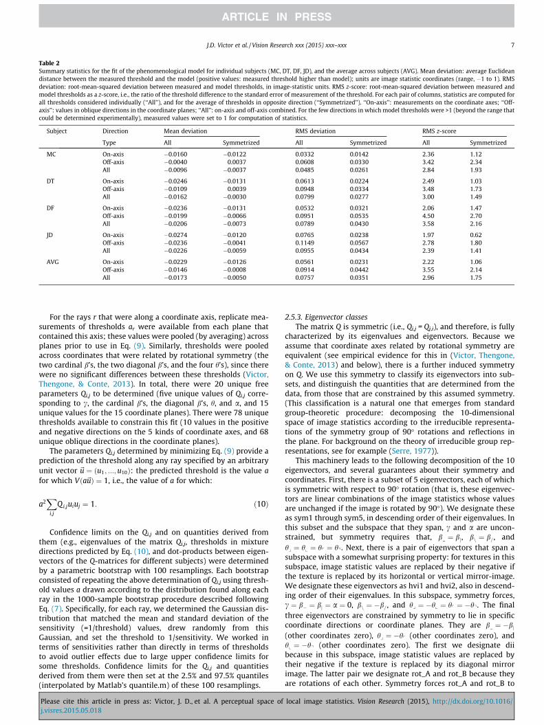
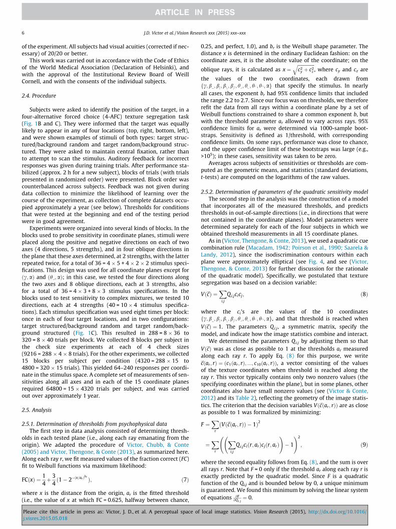
Table 2Summary statistics for the fit of the phenomenological model for individual subjects (MC, DT, DF, JD), and the average across subjects (AVG). Mean deviation: average Euclideandistance between the measured threshold and the model (positive values: measured threshold higher than model); units are image statistic coordinates (range, �1 to 1). RMSdeviation: root-mean-squared deviation between measured and model thresholds, in image-statistic units. RMS z-score: root-mean-squared deviation between measured andmodel thresholds as a z-score, i.e., the ratio of the threshold difference to the standard error of measurement of the threshold. For each pair of columns, statistics are computed forall thresholds considered individually (‘‘All’’), and for the average of thresholds in opposite direction (‘‘Symmetrized’’). ‘‘On-axis’’: measurements on the coordinate axes; ‘‘Off-axis’’: values in oblique directions in the coordinate planes; ‘‘All’’: on-axis and off-axis combined. For the few directions in which model thresholds were >1 (beyond the range thatcould be determined experimentally), measured values were set to 1 for computation of statistics.
Subject Direction Mean deviation RMS deviation RMS z-score
Type All Symmetrized All Symmetrized All Symmetrized
MC On-axis �0.0160 �0.0122 0.0332 0.0142 2.36 1.12Off-axis �0.0040 0.0037 0.0608 0.0330 3.42 2.34All �0.0096 �0.0037 0.0485 0.0261 2.84 1.93
DT On-axis �0.0246 �0.0131 0.0613 0.0224 2.49 1.03Off-axis �0.0109 0.0039 0.0948 0.0334 3.48 1.73All �0.0162 �0.0030 0.0799 0.0277 3.00 1.49
DF On-axis �0.0236 �0.0131 0.0532 0.0321 2.06 1.47Off-axis �0.0199 �0.0066 0.0951 0.0535 4.50 2.70All �0.0206 �0.0073 0.0789 0.0430 3.58 2.16
JD On-axis �0.0274 �0.0120 0.0765 0.0238 1.97 0.62Off-axis �0.0236 �0.0041 0.1149 0.0567 2.78 1.80All �0.0226 �0.0059 0.0955 0.0434 2.39 1.41
AVG On-axis �0.0229 �0.0126 0.0561 0.0231 2.22 1.06Off-axis �0.0146 �0.0008 0.0914 0.0442 3.55 2.14All �0.0173 �0.0050 0.0757 0.0351 2.96 1.75
J.D. Victor et al. / Vision Research xxx (2015) xxx–xxx 7
For the rays r that were along a coordinate axis, replicate mea-surements of thresholds ar were available from each plane thatcontained this axis; these values were pooled (by averaging) acrossplanes prior to use in Eq. (9). Similarly, thresholds were pooledacross coordinates that were related by rotational symmetry (thetwo cardinal b’s, the two diagonal b’s, and the four h’s), since therewere no significant differences between these thresholds (Victor,Thengone, & Conte, 2013). In total, there were 20 unique freeparameters Qi,j to be determined (five unique values of Qi,j corre-sponding to c, the cardinal b’s, the diagonal b’s, h, and a, and 15unique values for the 15 coordinate planes). There were 78 uniquethresholds available to constrain this fit (10 values in the positiveand negative directions on the 5 kinds of coordinate axes, and 68unique oblique directions in the coordinate planes).
The parameters Qi,j determined by minimizing Eq. (9) provide aprediction of the threshold along any ray specified by an arbitraryunit vector ~u ¼ ðu1; :::;u10Þ: the predicted threshold is the value afor which Vða~uÞ ¼ 1, i.e., the value of a for which:
a2X
i;j
Q i;juiuj ¼ 1: ð10Þ
Confidence limits on the Qi,j and on quantities derived fromthem (e.g., eigenvalues of the matrix Qi,j, thresholds in mixturedirections predicted by Eq. (10), and dot-products between eigen-vectors of the Q-matrices for different subjects) were determinedby a parametric bootstrap with 100 resamplings. Each bootstrapconsisted of repeating the above determination of Qi,j using thresh-old values a drawn according to the distribution found along eachray in the 1000-sample bootstrap procedure described followingEq. (7). Specifically, for each ray, we determined the Gaussian dis-tribution that matched the mean and standard deviation of thesensitivity (=1/threshold) values, drew randomly from thisGaussian, and set the threshold to 1/sensitivity. We worked interms of sensitivities rather than directly in terms of thresholdsto avoid outlier effects due to large upper confidence limits forsome thresholds. Confidence limits for the Qi,j and quantitiesderived from them were then set at the 2.5% and 97.5% quantiles(interpolated by Matlab’s quantile.m) of these 100 resamplings.
Please cite this article in press as: Victor, J. D., et al. A perceptual space ofj.visres.2015.05.018
2.5.3. Eigenvector classesThe matrix Q is symmetric (i.e., Qi,j = Qj,i), and therefore, is fully
characterized by its eigenvalues and eigenvectors. Because weassume that coordinate axes related by rotational symmetry areequivalent (see empirical evidence for this in (Victor, Thengone,& Conte, 2013) and below), there is a further induced symmetryon Q. We use this symmetry to classify its eigenvectors into sub-sets, and distinguish the quantities that are determined from thedata, from those that are constrained by this assumed symmetry.(This classification is a natural one that emerges from standardgroup-theoretic procedure: decomposing the 10-dimensionalspace of image statistics according to the irreducible representa-tions of the symmetry group of 90� rotations and reflections inthe plane. For background on the theory of irreducible group rep-resentations, see for example (Serre, 1977)).
This machinery leads to the following decomposition of the 10eigenvectors, and several guarantees about their symmetry andcoordinates. First, there is a subset of 5 eigenvectors, each of whichis symmetric with respect to 90� rotation (that is, these eigenvec-tors are linear combinations of the image statistics whose valuesare unchanged if the image is rotated by 90�). We designate theseas sym1 through sym5, in descending order of their eigenvalues. Inthis subset and the subspace that they span, c and a are uncon-strained, but symmetry requires that, b ¼ bj, bn ¼ b=, andhy ¼ hx ¼ hp ¼ hq. Next, there is a pair of eigenvectors that span asubspace with a somewhat surprising property: for textures in thissubspace, image statistic values are replaced by their negative ifthe texture is replaced by its horizontal or vertical mirror-image.We designate these eigenvectors as hvi1 and hvi2, also in descend-ing order of their eigenvalues. In this subspace, symmetry forces,c ¼ b� ¼ bj ¼ a ¼ 0, bn ¼ �b=, and hy ¼ �hx ¼ hp ¼ �hq. The finalthree eigenvectors are constrained by symmetry to lie in specificcoordinate directions or coordinate planes. They are b ¼ �bj(other coordinates zero), hy ¼ �hp (other coordinates zero), andhx ¼ �hq (other coordinates zero). The first we designate diibecause in this subspace, image statistic values are replaced bytheir negative if the texture is replaced by its diagonal mirrorimage. The latter pair we designate rot_A and rot_B because theyare rotations of each other. Symmetry forces rot_A and rot_B to
local image statistics. Vision Research (2015), http://dx.doi.org/10.1016/
8 J.D. Victor et al. / Vision Research xxx (2015) xxx–xxx
have the same eigenvalue. These final three eigenvectors are allwithin coordinate planes, and were therefore not used asout-of-sample tests of the model.
2.6. Previously reported work
A summary of findings for 4 subjects in 11 of the 15 planes atstandard check sizes is included in a paper that compares thesesensitivities to the statistics of natural images (Hermundstadet al., 2014). A partially overlapping portion of 6 subjects’ data in8 of those planes was also previously reported (Victor, Thengone,& Conte, 2013).
3. Results
3.1. Overview
Our immediate goal is to measure visual sensitivity to a set ofimage statistics chosen to capture the basic features of contrast,edge, and corner, and their interactions. As described in Methodsand (Victor & Conte, 2012), these statistics parameterize a10-dimensional space of black-and-white textures constructed ona square lattice. We begin with sensitivities to individual imagestatistics and then consider their pairwise interactions. Next, weuse these data to constrain a model for sensitivities to combina-tions of multiple image statistics, and we then test the model without-of-sample stimuli that contain such combinations. Finally, weshow how the above sensitivities, determined for a check size of14 min and a presentation time of 120 ms, change as a functionof these parameters.
3.2. Individual image statistics
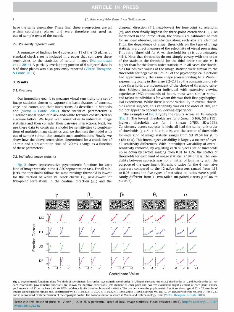
Fig. 2 shows representative psychometric functions for eachkind of image statistic in the 4-AFC segmentation task. For all sub-jects, the thresholds follow the same ranking: threshold is lowestfor the fraction of white vs. black checks (c), next-lowest fortwo-point correlations in the cardinal direction (b�) and the
+0.4-0.4 -0.4+0.2-0.2
MC1.0
.25
DT
JD
DF
γ β_
1.0
.25
1.0
.25
1.0
.25Frac
tion
Cor
rect
Coord0 -1 0 +1 0 0 -1 0 +1
Fig. 2. Psychometric functions along five kinds of coordinates: first-order ðcÞ, cardinal seceach coordinate, psychometric functions are shown for negative excursions (left elemperformance is 0.25; error bars indicate 95% confidence limits based on binomial statistimages along each coordinate axis, constructed with c ¼ �0:2, b� ¼ �0:4, b= ¼ �0:4, hy ¼and hy reproduced, with permission of the copyright holder, The Association for Researc
Please cite this article in press as: Victor, J. D., et al. A perceptual space ofj.visres.2015.05.018
diagonal direction (bn), next-lowest for four-point correlations,(a), and then finally highest for three-point correlations ðhyÞ. Asmentioned in the Introduction, the stimuli are calibrated so thatfor an ideal observer, sensitivities along each axis are identical.Thus, the dependence of visual thresholds on the type of imagestatistic is a direct measure of the selectivity of visual processing.This ratio (threshold for hy vs. threshold for c) is approximately4.5:1. Note that thresholds do not simply covary with the orderof the statistic: the threshold for the third-order statistic, hy, ishigher than for the fourth-order statistic, a. In all cases, the thresh-olds for positive values of the image statistic were similar to thethresholds for negative values. All of the psychophysical functionshad approximately the same shape (corresponding to a Weibullexponent typically in the range 2.2–2.7), so the comparisons of rel-ative thresholds are independent of the choice of threshold crite-rion. Subjects included an individual with extensive viewingexperience (MC: thousands of hours, most with similar stimuliand tasks) to individuals for whom this was their first psychophys-ical experiment. While there is some variability in overall thresh-olds across subjects, this variability was on the order of 20%, anddid not appear to depend on viewing experience.
The examples of Fig. 2 typify the results across all 16 subjects(Fig. 3). The lowest thresholds are for c (mean 0.166, SD ± 11%);highest thresholds are for hy (mean 0.793, SD ± 16%).Consistency across subjects is high: all had the same rank-orderof thresholds ðc < b� < bn < hy < aÞ, and the scatter of thresholdsfor each kind of image statistic ranges from SD ±9.5% for bn to±18% to a). This intersubject variability is largely a matter of over-all sensitivity differences. With intersubject variability of overallsensitivity removed, by adjusting each subject’s set of thresholdsup or down by factors ranging from 0.81 to 1.24, the scatter ofthresholds for each kind of image statistic is 10% or less. The vari-ability between subjects was not a matter of familiarity with thepurpose of the experiment (threshold ratios for the 4 non-naïveobservers compared to the 12 naïve observers ranged from 1.13to 0.93 across the five types of statistics; no ratios were signifi-cantly different from 1, two-tailed un-paired t-tests p = 0.06 top = 0.97).
+0.4 +0.8-0.8 +0.8-0.8
αθβ \ L
inate Value0 -1 0 +1 -1 0 +1 0 -1 0 +1
ond-order ðb Þ, diagonal second-order (b=), third-order ðhyÞ, and fourth-order ðaÞ. Forent of each pair) and positive excursions (right element of each pair). Chance
ics. The patches above the psychometric functions show typical 32 � 32 samples of�0:8, and a ¼ �0:8. Subjects MC, DT, JD, DF. Data for subjects MC and DT for b , b= ,h in Vision and Ophthalmology, from (Victor, Thengone, & Conte, 2013).
local image statistics. Vision Research (2015), http://dx.doi.org/10.1016/
Thre
shol
d
Texture Parameterγ αθβ_ β \
+ -+ -+ -+ -+ -0.1
1.0
0.2
0.5AA
AO
CC
MC
RM
DT
DF
JB
JD
KP
TT
JK
SR
RS
SP
DC
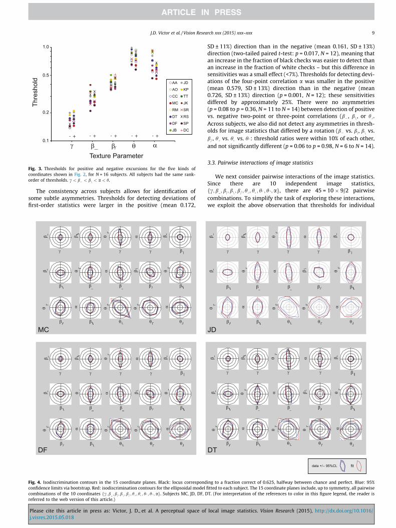
Fig. 3. Thresholds for positive and negative excursions for the five kinds ofcoordinates shown in Fig. 2, for N = 16 subjects. All subjects had the same rank-order of thresholds. c < b� < bn < a < h.
J.D. Victor et al. / Vision Research xxx (2015) xxx–xxx 9
The consistency across subjects allows for identification ofsome subtle asymmetries. Thresholds for detecting deviations offirst-order statistics were larger in the positive (mean 0.172,
γ γ γ β |γ
β _ β\
α β_θ
L
β _ α β\
β \ β_ β_ β \
θ
L
θ
L
β /
α αθ
L
θ
L
θ
L
β / β \ θ Lθ L θL
γ γ γ β |γ
β _ β\
α β_θ
L
β _ α β\
β \ β_ β_ β \
θ
L
θ
L
β /
α αθ
L
θ
L
θ
L
β / β \ θ Lθ L θL
MC
DF
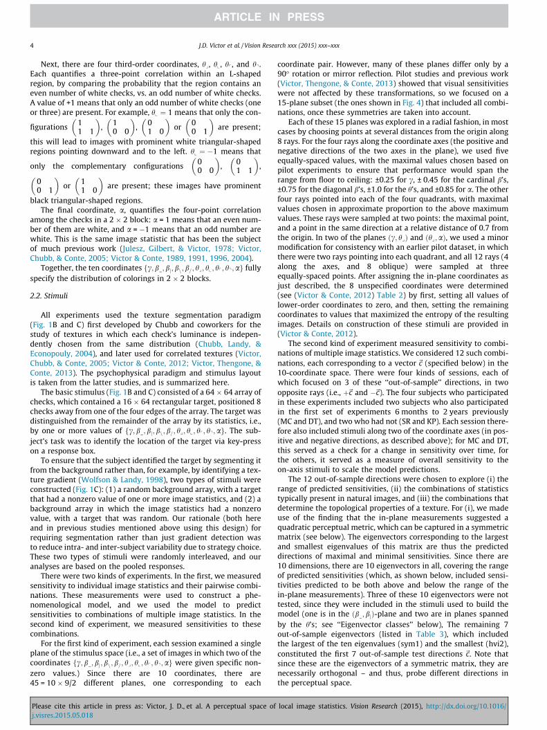
Fig. 4. Isodiscrimination contours in the 15 coordinate planes. Black: locus correspondconfidence limits via bootstrap. Red: isodiscrimination contours for the ellipsoidal modelcombinations of the 10 coordinates fc; b ; bj; bn; b=; hy; hx ; hp; hq ;ag. Subjects MC, JD, DF, Dreferred to the web version of this article.)
Please cite this article in press as: Victor, J. D., et al. A perceptual space ofj.visres.2015.05.018
SD ± 11%) direction than in the negative (mean 0.161, SD ± 13%)direction (two-tailed paired t-test: p = 0.017, N = 12), meaning thatan increase in the fraction of black checks was easier to detect thanan increase in the fraction of white checks – but this difference insensitivities was a small effect (<7%). Thresholds for detecting devi-ations of the four-point correlation a was smaller in the positive(mean 0.579, SD ± 13%) direction than in the negative (mean0.726, SD ± 13%) direction (p = 0.001, N = 12); these sensitivitiesdiffered by approximately 25%. There were no asymmetries(p = 0.08 to p = 0.36, N = 11 to N = 14) between detection of positivevs. negative two-point or three-point correlations (b�, bn, or hy.Across subjects, we also did not detect any asymmetries in thresh-olds for image statistics that differed by a rotation (b� vs. bj, bn vs.b=, hy vs. hx vs. hp: threshold ratios were within 10% of each other,and not significantly different (p = 0.06 to p = 0.98, N = 6 to N = 14).
3.3. Pairwise interactions of image statistics
We next consider pairwise interactions of the image statistics.Since there are 10 independent image statistics,fc; b ; bj; bn; b=; hy; hx; hp; hq;ag, there are 45 = 10 � 9/2 pairwisecombinations. To simplify the task of exploring these interactions,we exploit the above observation that thresholds for individual
data +/ - 95%CL fit
γ γ β |γ
β _ β\
β_θ
L
β _ α
β \ β_ β_ β \
θ
L
θ
L
α αθ
L
θ
L
β / β \ θ Lθ L
γ
αβ
\
β /
θ
L
θL
γ γ γ β |γ
β_
β\
α β_
θ
L
β _ α β\
β \ β_ β_ β \
θ
L
θ
L
β /
α αθ
L
θ
Lθ
L
β / β \ θ Lθ L θL
JD
DT
ing to a fraction correct of 0.625, halfway between chance and perfect. Blue: 95%fitted to each subject. The 15 coordinate planes include, up to symmetry, all pairwiseT. (For interpretation of the references to color in this figure legend, the reader is
local image statistics. Vision Research (2015), http://dx.doi.org/10.1016/
(dot
pro
duct
)
B 0.0
0.6
0.7
0.8
0.9
1.0
sym 1 sym 2 sym 3 sym 5sym 4 hvi 1 hvi 2
MC
DT
JD
DF
norm
alize
d
first order second order third order fourth order
-+
sym1 sym2 sym3 sym4 sym5 hvi1 hvi2 Ator BtoriidA
MC
DT
JD
DF
mean
1.0
0.8
0.6
0.4
0.2
0.0
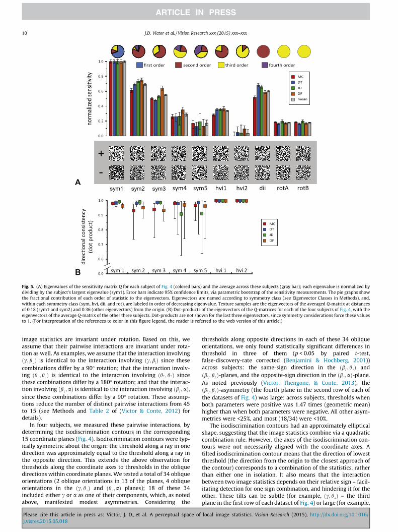
Fig. 5. (A) Eigenvalues of the sensitivity matrix Q for each subject of Fig. 4 (colored bars) and the average across these subjects (gray bar); each eigenvalue is normalized bydividing by the subject’s largest eigenvalue (sym1). Error bars indicate 95% confidence limits, via parametric bootstrap of the sensitivity measurements. The pie graphs showthe fractional contribution of each order of statistic to the eigenvectors. Eigenvectors are named according to symmetry class (see Eigenvector Classes in Methods), and,within each symmetry class (sym, hvi, dii, and rot), are labeled in order of decreasing eigenvalue. Texture samples are the eigenvectors of the averaged Q-matrix at distancesof 0.18 (sym1 and sym2) and 0.36 (other eigenvectors) from the origin. (B) Dot-products of the eigenvectors of the Q-matrices for each of the four subjects of Fig. 4, with theeigenvectors of the average Q-matrix of the other three subjects. Dot-products are not shown for the last three eigenvectors, since symmetry considerations force these valuesto 1. (For interpretation of the references to color in this figure legend, the reader is referred to the web version of this article.)
10 J.D. Victor et al. / Vision Research xxx (2015) xxx–xxx
image statistics are invariant under rotation. Based on this, weassume that their pairwise interactions are invariant under rota-tion as well. As examples, we assume that the interaction involvingðc; b Þ is identical to the interaction involving ðc; bjÞ since thesecombinations differ by a 90� rotation; that the interaction involv-ing ðhy; hxÞ is identical to the interaction involving ðhp; hqÞ sincethese combinations differ by a 180� rotation; and that the interac-tion involving ðbn;aÞ is identical to the interaction involving ðb=;aÞ,since these combinations differ by a 90� rotation. These assump-tions reduce the number of distinct pairwise interactions from 45to 15 (see Methods and Table 2 of (Victor & Conte, 2012) fordetails).
In four subjects, we measured these pairwise interactions, bydetermining the isodiscrimination contours in the corresponding15 coordinate planes (Fig. 4). Isodiscrimination contours were typ-ically symmetric about the origin: the threshold along a ray in onedirection was approximately equal to the threshold along a ray inthe opposite direction. This extends the above observation forthresholds along the coordinate axes to thresholds in the obliquedirections within coordinate planes. We tested a total of 34 obliqueorientations (2 oblique orientations in 13 of the planes, 4 obliqueorientations in the ðc; hyÞ and ðhy;aÞ planes); 18 of these 34included either c or a as one of their components, which, as notedabove, manifested modest asymmetries. Considering the
Please cite this article in press as: Victor, J. D., et al. A perceptual space ofj.visres.2015.05.018
thresholds along opposite directions in each of these 34 obliqueorientations, we only found statistically significant differences inthreshold in three of them (p < 0.05 by paired t-test,false-discovery-rate corrected (Benjamini & Hochberg, 2001))across subjects: the same-sign direction in the ðb=; hyÞ andðbn; b=Þ-planes, and the opposite-sign direction in the ðb ;aÞ-plane.As noted previously (Victor, Thengone, & Conte, 2013), theðbn; b=Þ-asymmetry (the fourth plane in the second row of each ofthe datasets of Fig. 4) was large: across subjects, thresholds whenboth parameters were positive was 1.47 times (geometric mean)higher than when both parameters were negative. All other asym-metries were <25%, and most (18/34) were <10%.
The isodiscrimination contours had an approximately ellipticalshape, suggesting that the image statistics combine via a quadraticcombination rule. However, the axes of the isodiscrimination con-tours were not necessarily aligned with the coordinate axes. Atilted isodiscrimination contour means that the direction of lowestthreshold (the direction from the origin to the closest approach ofthe contour) corresponds to a combination of the statistics, ratherthan either one in isolation. It also means that the interactionbetween two image statistics depends on their relative sign – facil-itating detection for one sign combination, and hindering it for theother. These tilts can be subtle (for example, ðc; hyÞ – the thirdplane in the first row of each dataset of Fig. 4) or large (for example,
local image statistics. Vision Research (2015), http://dx.doi.org/10.1016/
J.D. Victor et al. / Vision Research xxx (2015) xxx–xxx 11
ðhy; hxÞ – the third plane in the third row of each dataset of Fig. 4).To formalize this observation without postulating a specific shapefor the isodiscrimination contours, we compared thresholds forsame-sign vs.opposite-sign combinations of image statistics. Thisshowed that of the 15 planes, eight had contours with a significant(p < 0.05) tilt with respect to the axes (two-tailed paired t-testacross subjects, with false discovery rate correction.) In six planes,thresholds were lower for combinations of statistics that are of thesame sign, than for combinations that are of opposite sign, corre-sponding to a counterclockwise tilt: ðc; hyÞ, ðb�; bjÞ, ðb�;aÞ, ðbn; b=Þ,ðhy; hxÞ, and ðhy; hpÞ. In two planes, thresholds were higher forsame-sign combinations than for opposite-sign combinations,corresponding to a clockwise tilt: ðbn; hyÞ and ðb=; hyÞ.
3.4. A phenomenological model for interaction of image statistics
The results above indicate that isodiscrimination contours inthe coordinate planes had approximately elliptical shapes thatwere nearly symmetric with respect to the origin (i.e., that thresh-olds were similar along opposite rays), but were often tilted withrespect to the coordinate axes. Based on these observations, weframed a phenomenological model for how the image statisticsinteract to determine the perceptual threshold.
The basic idea is that the isodiscrimination contours form anellipse in each coordinate plane, and that these ellipses, takentogether, determine an ellipsoidal isodiscrimination contour inthe entire 10-dimensional space. In any single plane (e.g., a planecorresponding to coordinates cu and cv , where cu and cv are chosenfrom the 10 coordinates fc; b ; bj; bn; b=; hy; hx; hp; hq;ag), an ellipticalisodiscrimination contour can be described by the locus of pointsðcu; cv Þ where:
Q u;uc2u þ 2Qu;vcucv þ Qv;vc2
v ¼ 1: ð11Þ
The parameters Q describe the size and shape of the ellipse:1=
ffiffiffiffiffiffiffiffiffiQ u;u
pand 1=
ffiffiffiffiffiffiffiffiffiQv ;v
pare the thresholds for cu and cv , since
ð�1=ffiffiffiffiffiffiffiffiffiQu;u
p;0Þ and ð0;�1=
ffiffiffiffiffiffiffiffiffiQv ;v
pÞ are the points where the isodis-
crimination contour (11) intersects the axes. The third parameter,Q u;v , describes their interaction. We can then use a single equation,generalizing Eq. (11), to represent these contours in all coordinateplanes:X
i;j
Q i;jcicj ¼ 1: ð12Þ
Note that Eq. (12) simplifies to Eq. (11) in any plane (i.e., if onlytwo of the ck are nonzero). In Eq. (12), Qi;j is a symmetric matrix,
with 1=ffiffiffiffiffiffiffiQi:i
pcorresponding to the threshold along axis ci and
Q i;j ¼ Qj;i describing the interaction of ci and cj. Geometrically,Eq. (12) describes the unique 10-dimensional ellipsoid whoseintersection with each of the coordinate planes yields the ellipsesof Eq. (11). Q, a 10 � 10 symmetric matrix, has 20 independentparameters, since the symmetry considerations reduce the numberof unique diagonal elements to 5 (sensitivities for c, the cardinalb’s, the diagonal b’s, the h’s, and a), and the number of uniqueoff-diagonal elements to 15 (one for each coordinate plane ofFig. 4). There are 78 unique measured thresholds: the 10 on-axisthresholds, and 68 off-axis thresholds.
Fig. 4 shows the fit of this model in each of the planes, andTable 2 summarizes the statistics of the fit across subjects.Overall, the ellipsoidal shape provides a reasonable fit: theroot-mean-squared (RMS) error in thresholds is 0.076 across sub-jects (Table 2 bottom row, RMS deviation ‘‘all’’ column). The mainsource of model error is that there are modest differences inthresholds for positive and negative values of the image statistics(as noted above, a 25% lower threshold for a > 0 than for a < 0,
Please cite this article in press as: Victor, J. D., et al. A perceptual space ofj.visres.2015.05.018
smaller asymmetries for the other parameters). No quadraticmodel can account for such asymmetries. When the thresholds inopposite directions are replaced by their averaged values – so theeffect of this asymmetry is removed – the RMS error in the modelfit is 0.035 (Table 2 bottom row, RMS deviation ‘‘symmetrized’’column).
Though this error is small, we note that it is more than can beaccounted for from errors in the experimental measure of thresh-old. This is quantified via a z-score: the ratio of model error in eachdirection to the measurement error (1 s.d. of the bootstrapped dis-tribution of fitted thresholds). Root-mean-squared z-scores were2.95 for all thresholds, and 1.75 for the symmetrized thresholds,indicating that the model error is between 2 and 3-fold higher thancould be accounted for by the uncertainty of the psychophysicalmeasurements.
Most of this excess error can be attributed to the off-diagonalthresholds, i.e., to the model’s prediction of pairwise interactions.As seen in Table 2, the RMS z-score for the symmetrized thresholdswas 1.06 on-axis, indicating that the model error was only margin-ally larger than the uncertainty of psychophysical thresholds, butthe z-score was 2.14 off-axis, i.e., for the pairwise interactions.Overall, the phenomenological model slightly overestimatedon-axis thresholds, compared to off-axis thresholds (�0.023 com-pared to �0.015 considering all thresholds, �0.013 compared to�0.001 for the symmetrized thresholds).
In sum, while there are detectable systematic deviations of thephenomenological model from an ideal fit (there are asymmetriesof thresholds in opposite directions that account for model errorsof approximately 0.04 and there is a deviation from theclosest-fitting ellipsoidal shape that accounts for errors of 0.01–0.02), the model provides a reasonable summary of the shape ofthe isodiscrimination surfaces. We therefore use its parameters,the sensitivity matrix Q, to compare the shape of the isodiscrimina-tion surfaces across subjects, and, in the next section, to predictsensitivities for combinations of several image statistics.
Since Q is a symmetric matrix, we can use its eigenvalues andeigenvectors to compare it across subjects. Fig. 5A shows the eigen-values of the matrix Q determined from each of the four subjects,and the mean across subjects. Interestingly, the eigenvalue corre-sponding to the eigenvector hvi2 is experimentally indistinguish-able from 0 (its confidence limits include 0 for all subjects andthe cross-subject average). This means that the phenomenologicalmodel predicts that perceptual sensitivity is zero for this combina-tion of image statistics. Thus, the model predicts a combination ofimage statistics that is metameric to random – even though each ofthe image statistics, individually, is perceptually salient. This pre-diction will be tested below.
Fig. 5B compares the directions of the eigenvectors across sub-jects. All dot-products are close to 1, indicating that across the sub-jects, the principal axes of the ellipsoid (i.e., the directions ofgreatest and least sensitivities) are consistent.
3.5. Prediction of sensitivities for combinations of multiple imagestatistics
We next asked whether the phenomenological model, whichwas constructed to capture pairwise interactions of image statis-tics, could also account for more complex combinations. We testedthis with two kinds of out-of-sample measurements: first, withcombinations of statistics that were predicted to yield highestand lowest sensitivities, and second, combinations of statistics thatmight have functional importance, as they are associated withmaterial properties. The first set of combinations consists of theeigenvectors of the matrix Q determined above, and are listed inTable 3. One of these directions, hvi2, is of particular interest, sincethe predicted sensitivity in this direction is zero (Fig. 5). For the
local image statistics. Vision Research (2015), http://dx.doi.org/10.1016/
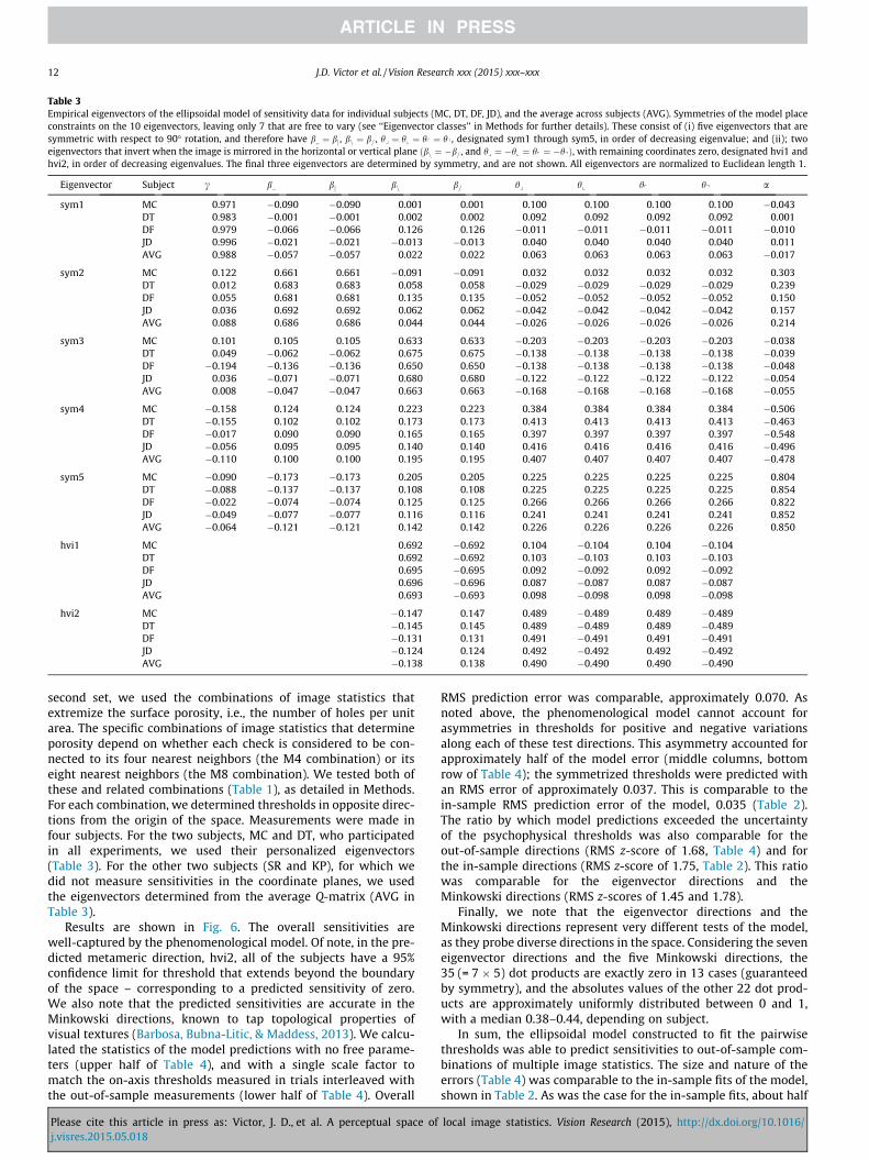
Table 3Empirical eigenvectors of the ellipsoidal model of sensitivity data for individual subjects (MC, DT, DF, JD), and the average across subjects (AVG). Symmetries of the model placeconstraints on the 10 eigenvectors, leaving only 7 that are free to vary (see ‘‘Eigenvector classes’’ in Methods for further details). These consist of (i) five eigenvectors that aresymmetric with respect to 90� rotation, and therefore have b ¼ bj , bn ¼ b= , hy ¼ hx ¼ hp ¼ hq , designated sym1 through sym5, in order of decreasing eigenvalue; and (ii); twoeigenvectors that invert when the image is mirrored in the horizontal or vertical plane ðbn ¼ �b= , and hy ¼ �hx ¼ hp ¼ �hqÞ, with remaining coordinates zero, designated hvi1 andhvi2, in order of decreasing eigenvalues. The final three eigenvectors are determined by symmetry, and are not shown. All eigenvectors are normalized to Euclidean length 1.
Eigenvector Subject c b bj bn b= hy hx hp hq a
sym1 MC 0.971 �0.090 �0.090 0.001 0.001 0.100 0.100 0.100 0.100 �0.043DT 0.983 �0.001 �0.001 0.002 0.002 0.092 0.092 0.092 0.092 0.001DF 0.979 �0.066 �0.066 0.126 0.126 �0.011 �0.011 �0.011 �0.011 �0.010JD 0.996 �0.021 �0.021 �0.013 �0.013 0.040 0.040 0.040 0.040 0.011AVG 0.988 �0.057 �0.057 0.022 0.022 0.063 0.063 0.063 0.063 �0.017
sym2 MC 0.122 0.661 0.661 �0.091 �0.091 0.032 0.032 0.032 0.032 0.303DT 0.012 0.683 0.683 0.058 0.058 �0.029 �0.029 �0.029 �0.029 0.239DF 0.055 0.681 0.681 0.135 0.135 �0.052 �0.052 �0.052 �0.052 0.150JD 0.036 0.692 0.692 0.062 0.062 �0.042 �0.042 �0.042 �0.042 0.157AVG 0.088 0.686 0.686 0.044 0.044 �0.026 �0.026 �0.026 �0.026 0.214
sym3 MC 0.101 0.105 0.105 0.633 0.633 �0.203 �0.203 �0.203 �0.203 �0.038DT 0.049 �0.062 �0.062 0.675 0.675 �0.138 �0.138 �0.138 �0.138 �0.039DF �0.194 �0.136 �0.136 0.650 0.650 �0.138 �0.138 �0.138 �0.138 �0.048JD 0.036 �0.071 �0.071 0.680 0.680 �0.122 �0.122 �0.122 �0.122 �0.054AVG 0.008 �0.047 �0.047 0.663 0.663 �0.168 �0.168 �0.168 �0.168 �0.055
sym4 MC �0.158 0.124 0.124 0.223 0.223 0.384 0.384 0.384 0.384 �0.506DT �0.155 0.102 0.102 0.173 0.173 0.413 0.413 0.413 0.413 �0.463DF �0.017 0.090 0.090 0.165 0.165 0.397 0.397 0.397 0.397 �0.548JD �0.056 0.095 0.095 0.140 0.140 0.416 0.416 0.416 0.416 �0.496AVG �0.110 0.100 0.100 0.195 0.195 0.407 0.407 0.407 0.407 �0.478
sym5 MC �0.090 �0.173 �0.173 0.205 0.205 0.225 0.225 0.225 0.225 0.804DT �0.088 �0.137 �0.137 0.108 0.108 0.225 0.225 0.225 0.225 0.854DF �0.022 �0.074 �0.074 0.125 0.125 0.266 0.266 0.266 0.266 0.822JD �0.049 �0.077 �0.077 0.116 0.116 0.241 0.241 0.241 0.241 0.852AVG �0.064 �0.121 �0.121 0.142 0.142 0.226 0.226 0.226 0.226 0.850
hvi1 MC 0.692 �0.692 0.104 �0.104 0.104 �0.104DT 0.692 �0.692 0.103 �0.103 0.103 �0.103DF 0.695 �0.695 0.092 �0.092 0.092 �0.092JD 0.696 �0.696 0.087 �0.087 0.087 �0.087AVG 0.693 �0.693 0.098 �0.098 0.098 �0.098
hvi2 MC �0.147 0.147 0.489 �0.489 0.489 �0.489DT �0.145 0.145 0.489 �0.489 0.489 �0.489DF �0.131 0.131 0.491 �0.491 0.491 �0.491JD �0.124 0.124 0.492 �0.492 0.492 �0.492AVG �0.138 0.138 0.490 �0.490 0.490 �0.490
12 J.D. Victor et al. / Vision Research xxx (2015) xxx–xxx
second set, we used the combinations of image statistics thatextremize the surface porosity, i.e., the number of holes per unitarea. The specific combinations of image statistics that determineporosity depend on whether each check is considered to be con-nected to its four nearest neighbors (the M4 combination) or itseight nearest neighbors (the M8 combination). We tested both ofthese and related combinations (Table 1), as detailed in Methods.For each combination, we determined thresholds in opposite direc-tions from the origin of the space. Measurements were made infour subjects. For the two subjects, MC and DT, who participatedin all experiments, we used their personalized eigenvectors(Table 3). For the other two subjects (SR and KP), for which wedid not measure sensitivities in the coordinate planes, we usedthe eigenvectors determined from the average Q-matrix (AVG inTable 3).
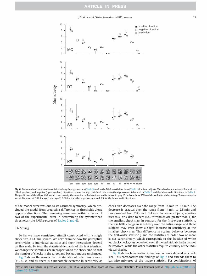
Results are shown in Fig. 6. The overall sensitivities arewell-captured by the phenomenological model. Of note, in the pre-dicted metameric direction, hvi2, all of the subjects have a 95%confidence limit for threshold that extends beyond the boundaryof the space – corresponding to a predicted sensitivity of zero.We also note that the predicted sensitivities are accurate in theMinkowski directions, known to tap topological properties ofvisual textures (Barbosa, Bubna-Litic, & Maddess, 2013). We calcu-lated the statistics of the model predictions with no free parame-ters (upper half of Table 4), and with a single scale factor tomatch the on-axis thresholds measured in trials interleaved withthe out-of-sample measurements (lower half of Table 4). Overall
Please cite this article in press as: Victor, J. D., et al. A perceptual space ofj.visres.2015.05.018
RMS prediction error was comparable, approximately 0.070. Asnoted above, the phenomenological model cannot account forasymmetries in thresholds for positive and negative variationsalong each of these test directions. This asymmetry accounted forapproximately half of the model error (middle columns, bottomrow of Table 4); the symmetrized thresholds were predicted withan RMS error of approximately 0.037. This is comparable to thein-sample RMS prediction error of the model, 0.035 (Table 2).The ratio by which model predictions exceeded the uncertaintyof the psychophysical thresholds was also comparable for theout-of-sample directions (RMS z-score of 1.68, Table 4) and forthe in-sample directions (RMS z-score of 1.75, Table 2). This ratiowas comparable for the eigenvector directions and theMinkowski directions (RMS z-scores of 1.45 and 1.78).
Finally, we note that the eigenvector directions and theMinkowski directions represent very different tests of the model,as they probe diverse directions in the space. Considering the seveneigenvector directions and the five Minkowski directions, the35 (= 7 � 5) dot products are exactly zero in 13 cases (guaranteedby symmetry), and the absolutes values of the other 22 dot prod-ucts are approximately uniformly distributed between 0 and 1,with a median 0.38–0.44, depending on subject.
In sum, the ellipsoidal model constructed to fit the pairwisethresholds was able to predict sensitivities to out-of-sample com-binations of multiple image statistics. The size and nature of theerrors (Table 4) was comparable to the in-sample fits of the model,shown in Table 2. As was the case for the in-sample fits, about half
local image statistics. Vision Research (2015), http://dx.doi.org/10.1016/
-+
m4 m8 m4+m8sym1 sym2 sym3 sym4 sym5 hvi1 hvi2 m4--m8 m6L-m6R
Sens
itivi
ty
0
2
4
6
8
10
0
2
4
6
8
10
0
2
4
6
8
10
0
2
4
6
8
10
positive directionnegative directionprediction
MC
DT
SR
KP
Fig. 6. Measured and predicted sensitivities along the eigenvectors (Table 3) and in the Minkowski directions (Table 1) for four subjects. Thresholds are measured for positive(filled symbols) and negative (open symbols) directions, where the sign is defined relative to the eigenvectors tabulated in Table 3 and the Minkowski directions in Table 1.The prediction of the ellipsoidal model is necessarily the same for both directions, and is shown in gray. Error bars show 95% confidence limits via bootstrap. Texture samplesare at distances of 0.18 for sym1 and sym2, 0.36 for the other eigenvectors, and 0.3 for the Minkowski directions.
J.D. Victor et al. / Vision Research xxx (2015) xxx–xxx 13
of the model error was due to its assumed symmetry, which pre-cluded the model from predicting differences in thresholds alongopposite directions. The remaining error was within a factor oftwo of the experimental error in determining the symmetrizedthresholds (the RMS z-scores of Tables 2 and 4).
3.6. Scaling
So far we have considered stimuli constructed with a singlecheck size, a 14-min square. We next examine how the perceptualsensitivities to individual statistics and their interactions dependon this scale. To keep the statistical demands of the task identical,we change the stimulus size in proportion to the check size, so thatthe number of checks in the target and background are unchanged.
Fig. 7 shows the results. For the statistics of order two or more(b�, bn, hy and a), there is a monotonic decrease in sensitivity as
Please cite this article in press as: Victor, J. D., et al. A perceptual space ofj.visres.2015.05.018
check size decreases over the range from 14 min to 1.4 min. Thedecrease is gradual over the range from 14 min to 2.8 min andmore marked from 2.8 min to 1.4 min. For some subjects, sensitiv-ities to hy or a drop to zero (i.e., thresholds are greater than 1) forthe smallest check size. In contrast, for the first-order statistic c,there is little change in sensitivity over the entire range, and threesubjects may even show a slight increase in sensitivity at thesmallest check size. This difference in scaling behavior betweenthe first-order statistic c and the statistics of order two or moreis not surprising: c, which corresponds to the fraction of whitevs. black checks, can be judged even if the individual checks cannotbe resolved, while the other statistics require visibility of the indi-vidual checks.
Fig. 8 shows how isodiscrimination contours depend on checksize. This corroborates the findings of Fig. 7 and extends them topairwise mixtures of the image statistics. For combinations of
local image statistics. Vision Research (2015), http://dx.doi.org/10.1016/
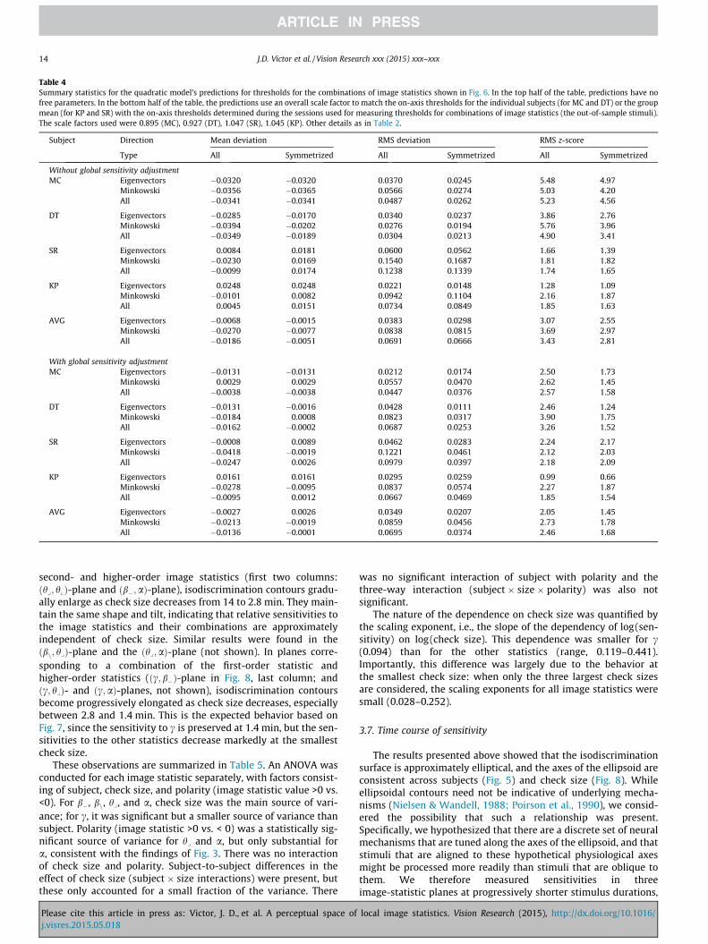
Table 4Summary statistics for the quadratic model’s predictions for thresholds for the combinations of image statistics shown in Fig. 6. In the top half of the table, predictions have nofree parameters. In the bottom half of the table, the predictions use an overall scale factor to match the on-axis thresholds for the individual subjects (for MC and DT) or the groupmean (for KP and SR) with the on-axis thresholds determined during the sessions used for measuring thresholds for combinations of image statistics (the out-of-sample stimuli).The scale factors used were 0.895 (MC), 0.927 (DT), 1.047 (SR), 1.045 (KP). Other details as in Table 2.
Subject Direction Mean deviation RMS deviation RMS z-score
Type All Symmetrized All Symmetrized All Symmetrized
Without global sensitivity adjustmentMC Eigenvectors �0.0320 �0.0320 0.0370 0.0245 5.48 4.97
Minkowski �0.0356 �0.0365 0.0566 0.0274 5.03 4.20All �0.0341 �0.0341 0.0487 0.0262 5.23 4.56
DT Eigenvectors �0.0285 �0.0170 0.0340 0.0237 3.86 2.76Minkowski �0.0394 �0.0202 0.0276 0.0194 5.76 3.96All �0.0349 �0.0189 0.0304 0.0213 4.90 3.41
SR Eigenvectors 0.0084 0.0181 0.0600 0.0562 1.66 1.39Minkowski �0.0230 0.0169 0.1540 0.1687 1.81 1.82All �0.0099 0.0174 0.1238 0.1339 1.74 1.65
KP Eigenvectors 0.0248 0.0248 0.0221 0.0148 1.28 1.09Minkowski �0.0101 0.0082 0.0942 0.1104 2.16 1.87All 0.0045 0.0151 0.0734 0.0849 1.85 1.63
AVG Eigenvectors �0.0068 �0.0015 0.0383 0.0298 3.07 2.55Minkowski �0.0270 �0.0077 0.0838 0.0815 3.69 2.97All �0.0186 �0.0051 0.0691 0.0666 3.43 2.81
With global sensitivity adjustmentMC Eigenvectors �0.0131 �0.0131 0.0212 0.0174 2.50 1.73
Minkowski 0.0029 0.0029 0.0557 0.0470 2.62 1.45All �0.0038 �0.0038 0.0447 0.0376 2.57 1.58
DT Eigenvectors �0.0131 �0.0016 0.0428 0.0111 2.46 1.24Minkowski �0.0184 0.0008 0.0823 0.0317 3.90 1.75All �0.0162 �0.0002 0.0687 0.0253 3.26 1.52
SR Eigenvectors �0.0008 0.0089 0.0462 0.0283 2.24 2.17Minkowski �0.0418 �0.0019 0.1221 0.0461 2.12 2.03All �0.0247 0.0026 0.0979 0.0397 2.18 2.09
KP Eigenvectors 0.0161 0.0161 0.0295 0.0259 0.99 0.66Minkowski �0.0278 �0.0095 0.0837 0.0574 2.27 1.87All �0.0095 0.0012 0.0667 0.0469 1.85 1.54
AVG Eigenvectors �0.0027 0.0026 0.0349 0.0207 2.05 1.45Minkowski �0.0213 �0.0019 0.0859 0.0456 2.73 1.78All �0.0136 �0.0001 0.0695 0.0374 2.46 1.68
14 J.D. Victor et al. / Vision Research xxx (2015) xxx–xxx
second- and higher-order image statistics (first two columns:ðhy; hxÞ-plane and ðb�;aÞ-plane), isodiscrimination contours gradu-ally enlarge as check size decreases from 14 to 2.8 min. They main-tain the same shape and tilt, indicating that relative sensitivities tothe image statistics and their combinations are approximatelyindependent of check size. Similar results were found in theðbn; hyÞ-plane and the ðhy;aÞ-plane (not shown). In planes corre-sponding to a combination of the first-order statistic andhigher-order statistics (ðc; b�Þ-plane in Fig. 8, last column; andðc; hyÞ- and ðc;aÞ-planes, not shown), isodiscrimination contoursbecome progressively elongated as check size decreases, especiallybetween 2.8 and 1.4 min. This is the expected behavior based onFig. 7, since the sensitivity to c is preserved at 1.4 min, but the sen-sitivities to the other statistics decrease markedly at the smallestcheck size.
These observations are summarized in Table 5. An ANOVA wasconducted for each image statistic separately, with factors consist-ing of subject, check size, and polarity (image statistic value >0 vs.<0). For b�, bn, hy, and a, check size was the main source of vari-ance; for c, it was significant but a smaller source of variance thansubject. Polarity (image statistic >0 vs. < 0) was a statistically sig-nificant source of variance for hy and a, but only substantial fora, consistent with the findings of Fig. 3. There was no interactionof check size and polarity. Subject-to-subject differences in theeffect of check size (subject � size interactions) were present, butthese only accounted for a small fraction of the variance. There
Please cite this article in press as: Victor, J. D., et al. A perceptual space ofj.visres.2015.05.018
was no significant interaction of subject with polarity and thethree-way interaction (subject � size � polarity) was also notsignificant.
The nature of the dependence on check size was quantified bythe scaling exponent, i.e., the slope of the dependency of log(sen-sitivity) on log(check size). This dependence was smaller for c(0.094) than for the other statistics (range, 0.119–0.441).Importantly, this difference was largely due to the behavior atthe smallest check size: when only the three largest check sizesare considered, the scaling exponents for all image statistics weresmall (0.028–0.252).
3.7. Time course of sensitivity
The results presented above showed that the isodiscriminationsurface is approximately elliptical, and the axes of the ellipsoid areconsistent across subjects (Fig. 5) and check size (Fig. 8). Whileellipsoidal contours need not be indicative of underlying mecha-nisms (Nielsen & Wandell, 1988; Poirson et al., 1990), we consid-ered the possibility that such a relationship was present.Specifically, we hypothesized that there are a discrete set of neuralmechanisms that are tuned along the axes of the ellipsoid, and thatstimuli that are aligned to these hypothetical physiological axesmight be processed more readily than stimuli that are oblique tothem. We therefore measured sensitivities in threeimage-statistic planes at progressively shorter stimulus durations,
local image statistics. Vision Research (2015), http://dx.doi.org/10.1016/
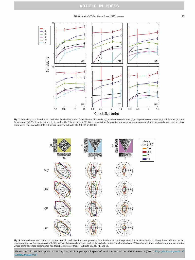
Fig. 7. Sensitivity as a function of check size for the five kinds of coordinates: first-order (c), cardinal second-order ðb Þ, diagonal second-order ðbnÞ, third-order ðhyÞ, andfourth-order (a). N = 6 subjects for c, b , hy , and a; N = 5 for bn (all but DT). For a, sensitivities for positive and negative excursions are plotted separately as aþ and a� , sincethese were systematically different across subjects. Subjects MC, SR, KP, SP, DT, RS.
MC
SR
KP
SP
γ
βθ
θ L
L α
β
checksize (min)
1.4 2.8 7 14
Fig. 8. Isodiscrimination contours as a function of check size for three pairwise combinations of the image statistics, in N = 4 subjects. Heavy lines indicate the locicorresponding to a fraction correct of 0.625, halfway between chance and perfect, for each check size. Thin lines indicate 95% confidence limits via bootstrap, and are omittedwhere some bootstrap resamplings had thresholds greater than 1. Subjects MC, SR, KP, and SP.
J.D. Victor et al. / Vision Research xxx (2015) xxx–xxx 15
Please cite this article in press as: Victor, J. D., et al. A perceptual space of local image statistics. Vision Research (2015), http://dx.doi.org/10.1016/j.visres.2015.05.018
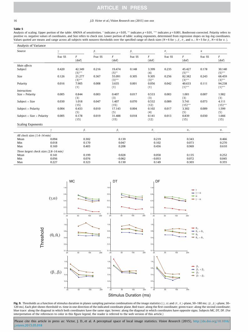
Table 5Analysis of scaling. Upper portion of the table: ANOVA of sensitivities. ⁄ indicates p < 0.05, ⁄⁄ indicates p < 0.01, ⁄⁄⁄ indicates p < 0.001, Bonferroni-corrected. Polarity refers topositive vs. negative values of coordinates, and Size refers to check size. Lower portion of table: scaling exponents, determined from regression slopes on log–log coordinates.Values quoted are means and range across all subjects with nonzero thresholds over the specified range of check sizes (N = 6 for c, b , hy , and aþ; N = 5 for bn , N = 4 for a�).
Analysis of Variance
Source c b� bn hy a
frac SS F Frac SS F frac SS F frac SS F frac SS F(dof) (dof) (dof) (dof) (dof)
Main effectsSubject 0.420 42.349 0.216 19.474 0.148 3.399 0.235 45.427 0.178 30.140
(5)⁄⁄⁄ (5)⁄⁄ (4) (5)⁄⁄⁄ (5)⁄⁄⁄
Size 0.126 21.277 0.367 55.091 0.305 9.305 0.256 82.382 0.243 68.459(3)⁄⁄⁄ (3)⁄⁄⁄ (3)⁄⁄ (3)⁄⁄⁄ (3)⁄⁄⁄
Polarity 0.016 7.905 0.008 3.635 0.001 0.056 0.042 40.633 0.111 94.238(1) (1) (1) (1)⁄⁄⁄ (1)⁄⁄⁄
InteractionsSize � Polarity 0.005 0.844 0.003 0.407 0.017 0.533 0.003 1.001 0.007 1.982
(3) (3) (3) (3) (3)Subject � Size 0.030 1.018 0.047 1.407 0.070 0.532 0.089 5.741 0.073 4.111
(15) (15) (12) (15)⁄⁄⁄ (15)⁄⁄⁄
Subject � Polarity 0.004 0.433 0.010 17.143 0.004 0.102 0.017 3.302 0.009 1.599(5) (5) (4) (5) (5)
Subject � Size � Polarity 0.005 0.178 0.019 31.488 0.018 0.141 0.013 0.839 0.030 1.666(15) (15) (12) (15) (15)
Scaling Exponents
c b� bn hy aþ a�
All check sizes (1.4–14 min)Mean 0.094 0.302 0.139 0.219 0.343 0.466Min 0.018 0.170 0.047 0.102 0.073 0.270Max 0.169 0.403 0.208 0.456 0.969 0.610
Three largest check sizes (2.8–14 min)Mean 0.141 0.199 0.028 0.058 0.135 0.252Min 0.056 0.076 �0.062 �0.053 0.072 0.045Max 0.227 0.323 0.130 0.149 0.303 0.355
0.1
0.2
0.4
0.8
1.6
25 50 100 2000.1
0.2
0.4
0.8
1.6
25 50 100 2000.1
0.2
0.4
0.8
1.6
25 50 100 200
0.1
0.2
0.4
0.8
1.6
25 50 100 2000.1
0.2
0.4
0.8
1.6
25 50 100 2000.1
0.2
0.4
0.8
1.6
25 50 100 200
0.1
0.2
0.4
0.8
1.6
25 50 100 2000.1
0.2
0.4
0.8
1.6
25 50 100 2000.1
0.2
0.4
0.8
1.6
25 50 100 200
MC DT DF
Stimulus Duration (ms)
Thre
shol
d
\
γγ + ααγ − α
θθ + θθθ − θ L
L
L
L
L
L
ββ + βββ − β
\
\
\
\
\\
(γ,α)
(θ ,θ )L L
(β , β )\
Fig. 9. Thresholds as a function of stimulus duration in planes sampling pairwise combinations of the image statistics (ðc;aÞ and ðhy; hxÞ-plane, 50–180 ms; ðbn; b=Þ-plane, 30–120 ms). Each plot shows threshold vs. time in one direction of the indicated coordinate plane. Red trace: along the first coordinate; green trace: along the second coordinate;blue trace: along the diagonal in which both coordinates have the same sign; brown: along the diagonal in which coordinates have opposite signs. Subjects MC, DT, DF. (Forinterpretation of the references to color in this figure legend, the reader is referred to the web version of this article.)
16 J.D. Victor et al. / Vision Research xxx (2015) xxx–xxx
Please cite this article in press as: Victor, J. D., et al. A perceptual space of local image statistics. Vision Research (2015), http://dx.doi.org/10.1016/j.visres.2015.05.018
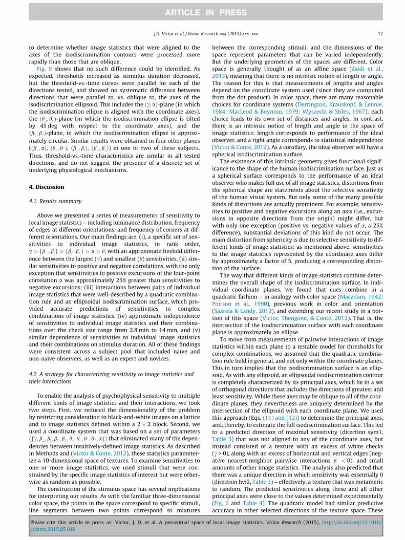
J.D. Victor et al. / Vision Research xxx (2015) xxx–xxx 17
to determine whether image statistics that were aligned to theaxes of the isodiscrimination contours were processed morerapidly than those that are oblique.
Fig. 9 shows that no such difference could be identified. Asexpected, thresholds increased as stimulus duration decreased,but the threshold-vs.-time curves were parallel for each of thedirections tested, and showed no systematic difference betweendirections that were parallel to, vs. oblique to, the axes of theisodiscrimination ellipsoid. This includes the ðc;aÞ-plane (in whichthe isodiscrimination ellipse is aligned with the coordinate axes),the ðhy; hxÞ-plane (in which the isodiscrimination ellipse is tiltedby 45 deg with respect to the coordinate axes), and theðbn; b=Þ-plane, in which the isodiscrimination ellipse is approxi-mately circular. Similar results were obtained in four other planes(ðb ;aÞ, ðhy; hpÞ, ðb ; bjÞ, ðb ; bnÞ) in one or two of these subjects.Thus, threshold-vs.-time characteristics are similar in all testeddirections, and do not suggest the presence of a discrete set ofunderlying physiological mechanisms.
4. Discussion
4.1. Results summary
Above we presented a series of measurements of sensitivity tolocal image statistics – including luminance distribution, frequencyof edges at different orientations, and frequency of corners at dif-ferent orientations. Our main findings are, (i), a specific set of sen-sitivities to individual image statistics, in rank order,c > fb�; bjg > fb=; bng > a > h, with an approximate fivefold differ-ence between the largest (c) and smallest (h) sensitivities, (ii) sim-ilar sensitivities to positive and negative correlations, with the onlyexception that sensitivities to positive excursions of the four-pointcorrelation a was approximately 25% greater than sensitivities tonegative excursions; (iii) interactions between pairs of individualimage statistics that were well-described by a quadratic combina-tion rule and an ellipsoidal isodiscrimination surface, which pro-vided accurate predictions of sensitivities to complexcombinations of image statistics, (iv) approximate independenceof sensitivities to individual image statistics and their combina-tions over the check size range from 2.8 min to 14 min, and (v)similar dependence of sensitivities to individual image statisticsand their combinations on stimulus duration. All of these findingswere consistent across a subject pool that included naïve andnon-naïve observers, as well as an expert and novices.
4.2. A strategy for characterizing sensitivity to image statistics andtheir interactions
To enable the analysis of psychophysical sensitivity to multipledifferent kinds of image statistics and their interactions, we tooktwo steps. First, we reduced the dimensionality of the problemby restricting consideration to black-and-white images on a latticeand to image statistics defined within a 2 � 2 block. Second, weused a coordinate system that was based on a set of parametersðfc; b ; bj; bn; b=; hy; hx; hp; hq;agÞ that eliminated many of the depen-dencies between intuitively-defined image statistics. As describedin Methods and (Victor & Conte, 2012), these statistics parameter-ize a 10-dimensional space of textures. To examine sensitivities toone or more image statistics, we used stimuli that were con-strained by the specific image statistics of interest but were other-wise as random as possible.
The construction of the stimulus space has several implicationsfor interpreting our results. As with the familiar three-dimensionalcolor space, the points in the space correspond to specific stimuli,line segments between two points correspond to mixtures
Please cite this article in press as: Victor, J. D., et al. A perceptual space ofj.visres.2015.05.018
between the corresponding stimuli, and the dimensions of thespace represent parameters that can be varied independently.But the underlying geometries of the spaces are different. Colorspace is generally thought of as an affine space (Zaidi et al.,2013), meaning that there is no intrinsic notion of length or angle.The reason for this is that measurements of lengths and anglesdepend on the coordinate system used (since they are computedfrom the dot product). In color space, there are many reasonablechoices for coordinate systems (Derrington, Krauskopf, & Lennie,1984; MacLeod & Boynton, 1979; Wyszecki & Stiles, 1967); eachchoice leads to its own set of distances and angles. In contrast,there is an intrinsic notion of length and angle in the space ofimage statistics: length corresponds to performance of the idealobserver, and a right angle corresponds to statistical independence(Victor & Conte, 2012). As a corollary, the ideal observer will have aspherical isodiscrimination surface.
The existence of this intrinsic geometry gives functional signif-icance to the shape of the human isodiscrimination surface. Just asa spherical surface corresponds to the performance of an idealobserver who makes full use of all image statistics, distortions fromthe spherical shape are statements about the selective sensitivityof the human visual system. But only some of the many possiblekinds of distortions are actually prominent. For example, sensitiv-ities to positive and negative excursions along an axis (i.e., excur-sions in opposite directions from the origin) might differ, butwith only one exception (positive vs. negative values of a, a 25%difference), substantial deviations of this kind do not occur. Themain distortion from sphericity is due to selective sensitivity to dif-ferent kinds of image statistics: as mentioned above, sensitivitiesto the image statistics represented by the coordinate axes differby approximately a factor of 5, producing a corresponding distor-tion of the surface.
The way that different kinds of image statistics combine deter-mines the overall shape of the isodiscrimination surface. In indi-vidual coordinate planes, we found that cues combine in aquadratic fashion – in analogy with color space (Macadam, 1942;Poirson et al., 1990), previous work in color and orientation(Saarela & Landy, 2012), and extending our recent study in a por-tion of this space (Victor, Thengone, & Conte, 2013). That is, theintersection of the isodiscrimination surface with each coordinateplane is approximately an ellipse.
To move from measurements of pairwise interactions of imagestatistics within each plane to a testable model for thresholds forcomplex combinations, we assumed that the quadratic combina-tion rule held in general, and not only within the coordinate planes.This in turn implies that the isodiscrimination surface is an ellip-soid. As with any ellipsoid, an ellipsoidal isodiscrimination contouris completely characterized by its principal axes, which lie in a setof orthogonal directions that includes the directions of greatest andleast sensitivity. While these axes may be oblique to all of the coor-dinate planes, they nevertheless are uniquely determined by theintersection of the ellipsoid with each coordinate plane. We usedthis approach (Eqs. (11) and (12)) to determine the principal axes,and, thereby, to estimate the full isodiscrimination surface. This ledto a predicted direction of maximal sensitivity (direction sym1,Table 3) that was not aligned to any of the coordinate axes, butinstead consisted of a texture with an excess of white checks(c > 0), along with an excess of horizontal and vertical edges (neg-ative nearest-neighbor pairwise interactions b� < 0), and smallamounts of other image statistics. The analysis also predicted thatthere was a unique direction in which sensitivity was essentially 0(direction hvi2, Table 3) – effectively, a texture that was metamericto random. The predicted sensitivities along these and all otherprincipal axes were close to the values determined experimentally(Fig. 6 and Table 4). The quadratic model had similar predictiveaccuracy in other selected directions of the texture space. These
local image statistics. Vision Research (2015), http://dx.doi.org/10.1016/
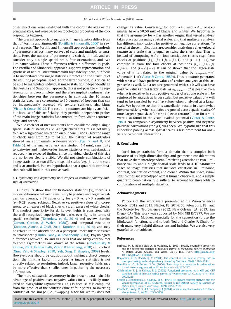
18 J.D. Victor et al. / Vision Research xxx (2015) xxx–xxx
other directions were unaligned with the coordinate axes or theprincipal axes, and were based on topological properties of the cor-responding textures.
The present approach to analysis of image statistics differs fromthat of Portilla and Simoncelli (Portilla & Simoncelli, 2000) in sev-eral respects. The Portilla and Simoncelli approach uses hundredsof parameters across many octaves of scale and multiple orienta-tions. Here, the number of parameters is strictly limited, and weconsider only a single spatial scale, four orientations, and twoluminance values. These differences reflect a difference in goals.The Portilla and Simoncelli approach supports representation andsynthesis of naturalistic textures with high fidelity; here, our focusis to understand how image statistics interact and the structure ofthe resulting perceptual space. For the latter purpose, it is crucial tobe able to manipulate individual image statistics independently. Inthe Portilla and Simoncelli approach, this is not possible – the rep-resentation is overcomplete, and there are implicit nonlinear rela-tionships between the parameters. In contrast, the 10 imagestatistics used here correspond to 10 degrees of freedom that canbe independently accessed via texture synthesis algorithms(Victor & Conte, 2012). The resulting textures are highly artificial,but because of this artificiality, they provide independent probesof the main image statistics fundamental to form vision (contrast,edge, and corner).
While each set of measurements here considered only a singlespatial scale of statistics (i.e., a single check size), this is not likelyto place a significant limitation on our conclusions. Over the rangeof check sizes from 2.8 to 14 min, the pattern of sensitivitiesshowed an approximate scale-invariance (Figs. 7 and 8, andTable 5). At the smallest check size studied (1.4 min), sensitivityto pairwise and higher-order image statistics was substantiallyreduced – an expected finding, since individual checks of this sizeare no longer clearly visible. We did not study combinations ofimage statistics at two different spatial scales (e.g., b� at one scaleand a at another), but we hypothesize that a quadratic combina-tion rule will hold in this case as well.
4.3. Symmetry and asymmetry with respect to contrast polarity andsign of correlation
Our results show that for first-order statistics (c), there is amodest difference between sensitivity to positive and negative val-ues: on average, a 7% superiority for c < 0 vs. c > 0, significant(p < 0.02) across subjects. Negative vs. positive values of c corre-spond to an excess of black checks vs. an excess of white checks.This modest superiority for darks over lights is consistent withthe well-recognized superiority for darks over lights in terms ofspatial resolution ((Kremkow et al., 2014) and review therein;(Zemon, Gordon, & Welch, 1988)), and temporal resolution(Komban, Alonso, & Zaidi, 2011; Komban et al., 2014), and maybe related to the observation of a perceptual mechanism sensitiveto ‘‘blackshot’’ (Chubb, Landy, & Econopouly, 2004). Physiologicaldifferences between ON and OFF cells that are likely contributorsto these asymmetries are known at the retinal (Chichilnisky &Kalmar, 2002; Pandarinath, Victor, & Nirenberg, 2010) and cortical(Xing, Yeh, & Shapley, 2010; Yeh, Xing, & Shapley, 2009) levels.However, one should be cautious about making a direct connec-tion: the limiting factor in processing image statistics is notdirectly related to resolution; indeed, larger receptive fields maybe more effective than smaller ones in gathering the necessaryinformation.
The more substantial asymmetry in the present data – the 25%advantage of positive over. negative values for a – is likely unre-lated to black/white asymmetries. This is because a is computedfrom the product of the contrast value at four points, so invertingcontrast of the image (i.e., swapping black for white) does not
Please cite this article in press as: Victor, J. D., et al. A perceptual space ofj.visres.2015.05.018
change its value. Conversely, for both a > 0 and a < 0, on-axisimages have a 50:50 mix of blacks and whites. We hypothesizethat the asymmetry for a has another origin: that visual analysistakes place across many spatial scales, and that multiscale analysishas different implications for positive vs. negative correlations. Tosee what these implications are, consider analyzing a checkerboardtexture at a scale that is equal to twice the check size. That is,instead of computing a from four contiguous checks (e.g., fromchecks at positions ði; jÞ, ðiþ 1; jÞ, ði; jþ 1Þ, and ðiþ 1; jþ 1Þ), wecompute it from the four checks at positions ði; jÞ, ðiþ 2; jÞ,ði; jþ 2Þ, and ðiþ 2; jþ 2Þ. It can be shown that the larger-scalevalue of a is related to the original value by alargescale ¼ a4
(Appendix 1 of (Victor & Conte, 1989)). Thus, a texture generatedwith a > 0 will have positive values of a when analyzed at this lar-ger scale as well. But, a texture generated with a < 0 will also havepositive values at this larger scale, as alargescale ¼ a4 is positive evenwhen a is negative. In sum, positive values of a at one scale will bereinforced by analysis at larger scales, but negative values of a willtend to be canceled by positive values when analyzed at a largerscale. We hypothesize that this cancellation results in a somewhatlower sensitivity when statistics are pooled across spatial scales. Ofnote, larger signal sizes for a = +1 (‘‘even texture’’) than for a = �1were also found in the visual evoked potential (Victor & Conte,1989). No comparable asymmetry between positive and negativepairwise correlations (the b’s) was seen. We hypothesize that thisis because pooling across spatial scales is less prominent for anal-ysis of two-point interactions.
5. Conclusion
Local image statistics form a domain that is complex bothbecause of its high dimensionality and geometric considerationsthat make them interdependent. Restricting attention to two lumi-nance values and a single spatial scale leads to a 10-parameterspace of image statistics that includes variations in luminance,contrast, orientation content, and corner. Within this space, visualsensitivities are stereotyped across human observers, and a simplequadratic combination rule suffices to account for thresholds tocombinations of multiple statistics.
Acknowledgments
Portions of this work were presented at the Vision SciencesSociety (2012 and 2013: Naples, FL; 2014: St. Petersburg, FL), andthe Society for Neuroscience (2012: New Orleans, LA; 2013: SanDiego, CA). This work was supported by NIH NEI EY7977. We aregrateful to Ted Maddess especially for the suggestion to use theMinkowski functionals, and to both Ted and Charles F. Chubb fortheir many very helpful discussions and insights. We are also verygrateful to our subjects.
References
Barbosa, M. S., Bubna-Litic, A., & Maddess, T. (2013). Locally countable propertiesand the perceptual salience of textures. Journal of the Optical Society of AmericaA: Optics, Image Science, and Vision, 30(8), 1687–1697. http://dx.doi.org/10.1364/JOSAA.30.001687.
Benjamini, Y., & Hochberg, Y. (2001). The control of the false discovery rate inmultiple testing under dependency. Annals of Statistics, 29(4), 1165–1188.
Ben-Shahar, O., & Zucker, S. W. (2004). Sensitivity to curvatures in orientation-based texture segmentation. Vision Research, 44, 257–277.
Chichilnisky, E. J., & Kalmar, R. S. (2002). Functional asymmetries in ON and OFFganglion cells of primate retina. Journal of Neuroscience, 22(7), 2737–2747. doi:20026215.
Chubb, C., Econopouly, J., & Landy, M. S. (1994). Histogram contrast analysis and thevisual segregation of IID textures. Journal of the Optical Society of America A:Optics, Image Science, and Vision, 11(9), 2350–2374.
Chubb, C., Landy, M. S., & Econopouly, J. (2004). A visual mechanism tuned to black.Vision Research, 44(27), 3223–3232.
local image statistics. Vision Research (2015), http://dx.doi.org/10.1016/
J.D. Victor et al. / Vision Research xxx (2015) xxx–xxx 19
Derrington, A. M., Krauskopf, J., & Lennie, P. (1984). Chromatic mechanisms inlateral geniculate nucleus of macaque. Journal of Physiology, 357, 241–265.
Doi, E., Balcan, D. C., & Lewicki, M. S. (2007). Robust coding over noisy overcompletechannels. IEEE Transactions on Image Processing, 16(2), 442–452.
Hermundstad, A. M., Briguglio, J. J., Conte, M. M., Victor, J. D., Balasubramanian, V., &Tkacik, G. (2014). Variance predicts salience in central sensory processing. eLife,3. http://dx.doi.org/10.7554/eLife. 03722.
Julesz, B., Gilbert, E. N., & Victor, J. D. (1978). Visual discrimination of textures withidentical third-order statistics. Biological Cybernetics, 31(3), 137–140.
Karklin, Y., & Lewicki, M. S. (2009). Emergence of complex cell properties bylearning to generalize in natural scenes. Nature, 457(7225), 83–86. http://dx.doi.org/10.1038/nature07481.
Komban, S. J., Alonso, J. M., & Zaidi, Q. (2011). Darks are processed faster than lights.Journal of Neuroscience, 31(23), 8654–8658. http://dx.doi.org/10.1523/JNEUROSCI.0504-11.2011.
Komban, S. J., Kremkow, J., Jin, J., Wang, Y., Lashgari, R., Li, X., et al. (2014).Neuronal and perceptual differences in the temporal processing of darksand lights. Neuron, 82(1), 224–234. http://dx.doi.org/10.1016/j.neuron.2014.02.020.
Kremkow, J., Jin, J., Komban, S. J., Wang, Y., Lashgari, R., Li, X., et al. (2014). Neuronalnonlinearity explains greater visual spatial resolution for darks than lights.Proceedings of the National academy of Sciences of the United States of America,111(8), 3170–3175. http://dx.doi.org/10.1073/pnas.1310442111.
Landy, M. S., & Oruc, I. (2002). Properties of second-order spatial frequencychannels. Vision Research, 42(19), 2311–2329.
Li, A., & Lennie, P. (1997). Mechanisms underlying segmentation of colored textures.Vision Research, 37(1), 83–97.
Macadam, D. L. (1942). Visual sensitivities to color differences in daylight. Journal ofthe Optical Society of America, 32, 247–273.
MacLeod, D. I., & Boynton, R. M. (1979). Chromaticity diagram showing coneexcitation by stimuli of equal luminance. The Journal of the Optical Society ofAmerica, 69(8), 1183–1186.
Michielsen, K., & De Raedt, H. (2001). Integral-geometry morphological imageanalysis. Physics Reports-Review Section of Physics Letters, 347(6), 462–538.
Motoyoshi, I., & Kingdom, F. A. A. (2007). Differential roles of contrast polarityreveal two streams of second-order visual processing. Vision Research, 2007,2047–2054.
Nielsen, K. R., & Wandell, B. A. (1988). Discrete analysis of spatial-sensitivitymodels. Journal of the Optical Society of America A: Optics, Image Science, andVision, 5(5), 743–755.
Pandarinath, C., Victor, J. D., & Nirenberg, S. (2010). Symmetry breakdown in the ONand OFF pathways of the retina at night: Functional implications. Journal ofNeuroscience, 30(30), 10006–10014. http://dx.doi.org/10.1523/JNEUROSCI.5616-09.2010.
Poirson, A., Wandell, B., Varner, D., & Brainard, D. (1990). Surface characterizationsof color thresholds. The Journal of the Optical Society of America, A7(783–789).
Please cite this article in press as: Victor, J. D., et al. A perceptual space ofj.visres.2015.05.018
Portilla, J., & Simoncelli, E. P. (2000). A parametric texture model based on jointstatistics of complex wavelet coefficients. International Journal of ComputerVision, 40(1), 49–71.
Saarela, T., & Landy, M. S. (2012). Combination of texture and color cues in visualsegmentation. Vision Research, 58, 59–67.
Serre, J.-P. (1977). Linear representations of finite groups. New York: Springer.Tkacik, G., Prentice, J. S., Victor, J. D., & Balasubramanian, V. (2010). Local statistics in
natural scenes predict the saliency of synthetic textures. Proceedings of theNational academy of Sciences of the United States of America, 107(42),18149–18154.
Victor, J. D., Chubb, C., & Conte, M. M. (2005). Interaction of luminance and higher-order statistics in texture discrimination. Vision Research, 45(3), 311–328.
Victor, J. D., & Conte, M. M. (1989). Cortical interactions in texture processing: Scaleand dynamics. Visual Neuroscience, 2(3), 297–313.
Victor, J. D., & Conte, M. M. (1991). Spatial organization of nonlinear interactions inform perception. Vision Research, 31(9), 1457–1488.
Victor, J. D., & Conte, M. M. (1996). The role of high-order phase correlations intexture processing. Vision Research, 36(11), 1615–1631.
Victor, J. D., & Conte, M. M. (2004). Visual working memory for image statistics.Vision Research, 44(6), 541–556.
Victor, J. D., & Conte, M. M. (2012). Local image statistics: Maximum-entropyconstructions and perceptual salience. Journal of the Optical Society of America A:Optics, Image Science, and Vision, 29(7), 1313–1345. http://dx.doi.org/10.1364/JOSAA.29.001313.
Victor, J. D., Thengone, D. J., & Conte, M. M. (2013). Perception of second- and third-order orientation signals and their interactions. Journal of Vision, 13(4), 21.http://dx.doi.org/10.1167/13.4.21.
Wolfson, S. S., & Landy, M. S. (1995). Discrimination of orientation-defined textureedges. Vision Research, 35(20), 2863–2877.
Wolfson, S. S., & Landy, M. S. (1998). Examining edge- and region-based textureanalysis mechanisms. Vision Research, 38, 439–446.
Wyszecki, G., & Stiles, W. (1967). Color science: Concepts and methods, quantitativedata and formulas. New York: Wiley.
Xing, D., Yeh, C. I., & Shapley, R. M. (2010). Generation of black-dominant responsesin V1 cortex. Journal of Neuroscience, 30(40), 13504–13512. http://dx.doi.org/10.1523/JNEUROSCI.2473-10.2010.
Yeh, C. I., Xing, D., & Shapley, R. M. (2009). ‘‘Black’’ responses dominate macaqueprimary visual cortex v1. Journal of Neuroscience, 29(38), 11753–11760. http://dx.doi.org/10.1523/JNEUROSCI.1991-09.2009.
Zaidi, Q., Victor, J., McDermott, J., Geffen, M., Bensmaia, S., & Cleland, T. A. (2013).Perceptual spaces: Mathematical structures to neural mechanisms. Journal ofNeuroscience, 33(45), 17597–17602. http://dx.doi.org/10.1523/jneurosci.3343-13.2013.
Zemon, V., Gordon, J., & Welch, J. (1988). Asymmetries in ON and OFF visualpathways of humans revealed using contrast-evoked cortical potentials. VisualNeuroscience, 1(1), 145–150.
local image statistics. Vision Research (2015), http://dx.doi.org/10.1016/


![Perceptual Evaluation of Color-to-Grayscale Image Conversions€¦ · – [Smith et al. 08] Perceptual Evaluation of Color-to-Grayscale Image Conversions, Martin adík, cadikm@fel.cvut.cz](https://img.pdfslide.net/doc/110x75/6027c8392fd6cd755c692258/perceptual-evaluation-of-color-to-grayscale-image-conversions-a-smith-et-al.jpg)


![A transformation-aware perceptual image metric [9394-5] · A transformation-aware perceptual image metric Petr Kellnhofer a Tobias Ritschel a,b Karol Myszkowski a Hans-Peter Seidel](https://img.pdfslide.net/doc/110x75/5f870db3183b296e7525af0a/a-transformation-aware-perceptual-image-metric-9394-5-a-transformation-aware-perceptual.jpg)