A PERMUTATION TEST FOR THE STRUCTURE

OF A COVARIANCE MATRIX

By

TRACY LYNNE MORRIS

Bachelor of Science in Mathematics Oklahoma State University

Stillwater, Oklahoma 1994

Master of Science in Applied Mathematical Sciences University of Central Oklahoma

Edmond, Oklahoma 2001

Submitted to the Faculty of the Graduate College of the

Oklahoma State University in partial fulfillment of

the requirements for the Degree of

DOCTOR OF PHILOSOPHY May, 2007

ii

A PERMUTATION TEST FOR THE STRUCTURE

OF A COVARIANCE MATRIX

Dissertation Approved:

Dr. Mark Payton

Dissertation Adviser Dr. William Warde

Dr. Stephanie Monks

Dr. Douglas Aichele

Dr. A. Gordon Emslie

Dean of the Graduate College

iii

ACKNOWLEDGMENTS

I would like to express my sincere gratitude to Dr. Mark Payton for his support,

expertise, encouragement, and advice, without which I would not have been able to

complete this dissertation. I would also like to thank the other members of my

committee, Dr. William Warde, Dr. Stephanie Monks, and Dr. Douglas Aichele, for

reviewing my work and providing invaluable guidance. Finally, I would like to extend

my gratitude to the entire Department of Statistics.

Special thanks also goes to Dr. Mauricio Subieta and the High Performance

Computing Center. Without Dr. Subieta’s help and the use of the computing center I

would undoubtedly be running simulations for many months to come.

Finally, I would like to thank my family and friends for their support. I am

especially thankful for my husband, Mark, and my mother, Kay, for their loving

encouragement and emotional support throughout this process.

iv

TABLE OF CONTENTS

Chapter Page 1. INTRODUCTION ....................................................................................................1

2. PARAMETRIC TESTS FOR THE STRUCTURE OF A COVARIANCE MATRIX...............................................................................................................3

2.1 Tests of Sphericity .........................................................................................5 2.2 Test of Compound Symmetry......................................................................10 2.3 Test of Type H Structure..............................................................................13 2.4 Test of Serial Correlation.............................................................................15 2.5 Test of Independence of Sets of Variates ....................................................19 2.6 Factor Analysis / Structural Equation Modeling .........................................21

3. BOOTSTRAPPING................................................................................................26

4. PERMUTATION TESTS .......................................................................................28

5. PROPOSED TEST..................................................................................................33

5.1 Permutation Tests of Sphericity and Compound Symmetry........................34 5.2 Permutation Test of Type H Structure .........................................................38 5.3 Permutation Test of All Other Covariance Structures .................................40

6. SIMULATIONS .....................................................................................................45

6.1 Test of Sphericity.........................................................................................50 6.2 Test of Compound Symmetry......................................................................63 6.3 Test of Type H Structure..............................................................................73 6.4 Test of Serial Correlation.............................................................................81 6.5 Test of Independence of Sets of Variates ....................................................92

7. CONCLUSIONS...................................................................................................100

v

8. FUTURE WORK..................................................................................................102

BIBLIOGRAPHY......................................................................................................105

APPENDIX................................................................................................................111

A.1 R Code.......................................................................................................111 A.1.1 Randomization Test of Sphericity.................................................111 A.1.2 Randomization Test of Compound Symmetry..............................118 A.1.3 Permutation Test of Type H Structure ..........................................125 A.1.4 Randomization Test of Type H Structure .....................................132 A.1.5 Randomization Test of Serial Correlation ....................................139 A.1.6 Randomization Test of Independence of Sets of Variates ............149 A.1.7 Randomization Test of Independence of Sets of Variates for n=5 and (5,5)............................................................................157 A.2 Combinations of d and γ used in the Type H Simulations........................162 A.3 Bias Correction for the Serial Correlation Parameters..............................166

A.4 Number of Simulated Data Sets for the Test of Independence of Sets of Variates for n=5 and (5,5)..................................................................180

vi

LIST OF TABLES

Table Page 4.0.1 All Possible Permutations of the Observed Data...................................................29 5.1.1 Observed Data........................................................................................................36 5.1.2 Some Permutations of the Centered Observed Data..............................................37 6.1.1 Simulated Type I Error Rates for the Test of Sphericity .......................................52 6.1.2 Simulated Power vs. Non-Homoscedasticity for the Test of Sphericity ...............54 6.1.3 Simulated Power vs. Non-Zero Correlation for the Test of Sphericity .................56 6.1.4 Simulated Power vs. Type H for the Test of Sphericity (p=3) ..............................58 6.1.5 Simulated Power vs. Type H for the Test of Sphericity (p=5) ..............................59 6.1.6 Simulated Power vs. Type H for the Test of Sphericity (p=10) ............................60 6.1.7 Simulated Power vs. Serial Correlation for the Test of Sphericity ( 2 1σ = ) .........62 6.2.1 Simulated Type I Error Rates for the Test of Compound Symmetry (p=3) ..........64 6.2.2 Simulated Type I Error Rates for the Test of Compound Symmetry (p=5) ..........65 6.2.3 Simulated Type I Error Rates for the Test of Compound Symmetry (p=10) ........66 6.2.4 Simulated Power vs. Type H for the Test of Compound Symmetry (p=3) ...........68 6.2.5 Simulated Power vs. Type H for the Test of Compound Symmetry (p=5) ...........69 6.2.6 Simulated Power vs. Type H for the Test of Compound Symmetry (p=10) .........70 6.2.7 Simulated Power vs. Serial Correlation for the Test of Compound Symmetry ( 2 1σ = ) ............................................................................................................72 6.3.1 Simulated Type I Error Rates for the Test of Type H (p=3)..................................74

vii

6.3.2 Simulated Type I Error Rates for the Test of Type H (p=5)..................................75 6.3.3 Simulated Type I Error Rates for the Test of Type H (p=10)................................76 6.3.4 Simulated Power vs. Serial Correlation for the Test of Type H (p=3) ..................78 6.3.5 Simulated Power vs. Serial Correlation for the Test of Type H (p=5) ..................79 6.3.6 Simulated Power vs. Serial Correlation for the Test of Type H (p=10) ................80 6.4.1 Simulated Type I Error Rates for the Test of Serial Correlation (p=3) .................83 6.4.2 Simulated Type I Error Rates for the Test of Serial Correlation (p=5) .................84 6.4.3 Simulated Type I Error Rates for the Test of Serial Correlation (p=10) ...............85 6.4.4 Simulated Power vs. Compound Symmetry for the Test of Serial Correlation ( 2 1σ = ) ............................................................................................................87 6.4.5 Simulated Power vs. Type H for the Tets of Serial Correlation (p=3) ..................89 6.4.6 Simulated Power vs. Type H for the Tets of Serial Correlation (p=5) ..................90 6.4.7 Simulated Power vs. Type H for the Tets of Serial Correlation (p=10) ................91 6.5.1 Simulated Type I Error Rates for the Test of Independence of Sets of Variates...96 6.5.2 Simulated Power vs. Non-Independence for the Test of Independence of Sets of Variates........................................................................................................99 A.2.1 Combinations of d and γ Used in the Simulations...............................................165 A.3.1 Simulated Values of K ........................................................................................172 A.3.2 Simulated Type I Error Rates for the Test of Serial Correlation with Normally Distributed Data and p=3...............................................................................174 A.4.1 Number of Data Sets Simulated for the Test of Independence of Sets of Variates for n=5 and (5,5) ............................................................................................180

viii

LIST OF FIGURES Figure Page 2.4.1 General Plot of ( )ρ̂f ............................................................................................18 5.1.1 Distribution of the Test Statistic for Compound Symmetry ..................................38 5.3.1 Distribution of the Test Statistic for Serial Correlation .........................................44 A.2.1 Regions of Possible Combinations of d and γ .....................................................164 A.3.1 Bias of the MLEs of ρ and 2σ .............................................................................167

A.3.2 Bias of 2*σ̂ and 2

*ˆ1

nn

σ−

.......................................................................................169

A.3.3 Scatterplots of K and nK ...................................................................................173

1

CHAPTER 1

INTRODUCTION

Many statistical procedures, including repeated measures analysis, time-series,

structural equation modeling, and factor analysis, require an assessment of the structure

of the covariance matrix of the measurements. For example, consider a repeated

measures experiment in which researchers are interested in the effect of various teaching

strategies on reading. Throughout the course of the experiment, reading tests are given to

children at various time periods and the multiple test scores are recorded for each student.

Repeated measurements taken on subjects tend to be correlated; consequently, the

assumption of independent observations required by a univariate analysis of variance

(ANOVA) is violated. However, Huynh and Feldt (1970) showed that if the structure of

the covariance matrix is of the same form as a type H matrix (described in Section 2.3), a

univariate ANOVA can be used. If the covariance matrix is not type H, an alternate

analysis must be employed. Therefore, it is necessary to determine the structure of the

covariance matrix to know how to proceed with the analysis.

The classical parametric method of testing the hypothesis 0=Σ Σ , where 0Σ is

some hypothesized covariance structure, involves the use of a likelihood ratio test

statistic that converges in distribution to a chi-squared random variable. This test has

many limitations, including the need for very large sample sizes and the requirement of a

random sample from a multivariate normal population. It is quite reasonable to think of

2

many situations in which at least one of these conditions is violated. For example, in

educational and medical studies, researchers frequently rely on volunteers, violating the

assumption of a random sample; in psychological studies, responses are often recorded

on Likert scales, violating the assumption of multivariate normality; and in studies in

which experimental units are rare or costly, researchers are restricted to very small

sample sizes. In situations in which only some or none of these assumptions are met,

researchers could benefit from a non-parametric testing procedure. In particular,

permutation tests have no distributional assumptions, do not require random samples, and

allow any sample size.

The objectives of this research are to develop a permutation testing procedure to

test the null hypothesis, 0=Σ Σ , and to investigate the empirical type I error rates and

power of this test against various alternative structures. In the following chapters, I will

present the motivation for developing such a test. Specifically, in Chapter 2, I will

describe the parametric procedures for testing the structure of a covariance matrix,

including a discussion of their benefits and limitations; in Chapter 3, I will briefly discuss

the use of bootstrapping for estimating or testing the covariance structure; in Chapter 4, I

will review the general history and development of permutation tests, including a

description of the differences between permutation tests and bootstrapping; in Chapter 5,

I will propose a permutation test for the structure of a covariance matrix and will argue as

to why such a test would be appropriate and necessary; in Chapter 6, I will describe the

evaluation of the proposed test using simulations; in Chapter 7, I will summarize the

overall conclusions; and finally, in Chapter 8, I will list some future research questions.

3

CHAPTER 2

PARAMETRIC TESTS FOR THE STRUCTURE OF A COVARIANCE MATRIX

The classical approach to testing the structure of a covariance matrix involves the

use of a likelihood ratio test statistic. Let ix , 1, ,i n= K , be p-component vectors

distributed according to ( , )pN µ Σ , where Σ is positive definite and n p> . The

likelihood ratio criterion for testing 0 0:H =Σ Σ versus 0:aH ≠Σ Σ can be found by

computing the ratio of the likelihood maximized under the null hypothesis (i.e. with

respect to µ and 0Σ ) to the likelihood maximized under the alternative hypothesis (i.e.

with respect to µ and an unrestricted positive definite Σ ). The likelihood function under

the alternative hypothesis is given by

( ) ( )22 112

1

(2 ) expn

nnpi i

iL −− −

=

′= π − − − ∑Σ x µ Σ x µ

and the corresponding log likelihood function is

( ) ( )11 1 12 2 2

1log log(2 ) log

n

i ii

L np n −

=

′= − π − − − −∑Σ x µ Σ x µ , (2.0.1)

where log is assumed base e. Since log L is an increasing function of L, the values that

maximize (2.0.1) are equivalent to the values that maximize L. To maximize (2.0.1) with

respect to µ and Σ , consider the following lemma given by Anderson (2003).

4

Lemma 2.0.1. Let ix , 1, ,i n= K , be p-component vectors, and let x be the

corresponding sample mean vector. Then for any vector b

( )( ) ( ) ( ) ( )( )1 1

n n

i i i ii i

n= =

′ ′ ′− − = − − + − −∑ ∑x b x b x x x x x b x b .

Applying the properties of the trace of a matrix (tr(•)) and lemma 2.0.1 to just the last

term of (2.0.1) gives

( ) ( ) ( ) ( )

( )( )

( )( ) ( )( )

( )( ) ( ) ( )

1 1

1 1

1

1

1 1

1

1 1

1

tr

tr

tr tr

tr .

n n

i i i ii i

n

i ii

n

i ii

n

i ii

n

n

− −

= =

−

=

− −

=

− −

=

′ ′− − = − − ′= − − ′ ′= − − + − − ′ ′= − − + − −

∑ ∑

∑

∑

∑

x µ Σ x µ x µ Σ x µ

Σ x µ x µ

Σ x x x x Σ x µ x µ

Σ x x x x x µ Σ x µ

Therefore, (2.0.1) can be written as

( ) ( ) ( ) ( )

1 12 2

1 11 12 2

1

log log(2 ) log

tr .n

i ii

L np n

n− −

=

= − π −

′ ′− − − − − − ∑

Σ

Σ x x x x x µ Σ x µ(2.0.2)

To maximize log L with respect to µ , it is only necessary to consider the last term

of (2.0.2). Since Σ is positive definite, 1−Σ is also positive definite. Therefore,

( ) ( )112 0n −′− − − ≤x µ Σ x µ and is maximized at 0 if and only if =µ x . Consequently,

the maximum likelihood estimate (MLE) of µ is ˆ =µ x . Substituting x for µ , (2.0.2)

simplifies to

( )( )11 1 12 2 2

1

log log(2 ) log tr .n

i ii

L np n −

=

′= − π − − − − ∑Σ Σ x x x x (2.0.3)

5

To find the MLE of Σ , consider another lemma given by Anderson (2003).

Lemma 2.0.2. If D is positive definite of order p, the maximum of

( )1( ) log trf n −= − −G G G D

with respect to positive definite matrices G exists and occurs at ( )1 n=G D .

To maximize (2.0.3) with respect to Σ it is only necessary to consider the second and

third terms. Applying lemma 2.0.2 to these terms gives the MLE of Σ ,

( )( )1

1ˆn

i iin =

′= − −∑Σ x x x x .

These MLEs for µ and Σ along with the MLEs found under various null

hypotheses can be used to compute likelihood ratio statistics for parametrically testing the

structure of a covariance matrix. Specific test statistics for various covariance structures

are outlined in the sections to follow.

2.1 TESTS OF SPHERICITY

Consider first the test of sphericity proposed by Mauchly (1940). A p-variate

population is called spherical if the variances of the variables are all equal and the

pairwise correlations among the variables are all zero. Specifically, this is a test of the

null hypothesis 2S p= σΣ I , where pI is the p p× identity matrix and 2σ is the

hypothesized common variance among the variables. This hypothesis applies to many

univariate procedures, such as ANOVA, in which it is assumed that a set of random

6

variables are independent and have a common variance. To test this assumption, the

likelihood ratio criterion given by

( )( )

2,

,

max ,

max ,

S

S

L

Lσλ = µ

µ Σ

µ Σ

µ Σ

can be computed. As shown previously, the MLE of µ does not depend on the specific

form of Σ ; therefore, the MLEs of µ and Σ , in both the numerator and denominator of

Sλ , are given by

ˆ =µ x and ( )( )1

1ˆn

i iin =

′= − −∑Σ x x x x .

To find the MLE of 2σ , consider the following. Under the null hypothesis, the

log likelihood function is

( ) ( )221 1 1

2 2 21

log log(2 ) logn

S i ii

L np npσ

=

′= − π − σ − − −∑ x µ x µ (2.1.1)

and the partial derivative of (2.1.1) with respect to 2σ is

( ) ( )2 2 41

log 12 2

nS

i ii

L np=

∂ ′= − + − −∂σ σ σ ∑ x µ x µ . (2.1.2)

Substituting x for µ and setting (2.1.2) equal to 0 gives the MLE of 2σ ,

( ) ( )2

1

1ˆn

i iinp =

′σ = − −∑ x x x x .

Then, the likelihood ratio criterion for testing 2S p= σΣ I becomes

( ) ( ) ( )

( ) ( ) ( )

122 2 21 22

12222 11

21

ˆ ˆ(2 ) exp ˆ

ˆˆ ˆ(2 ) exp

nnnp ni i

iS npnnnp

i ii

−−−

=

−− −

=

=

′π σ − − σ − λ = σ′π − − −

∑

∑

I x x I x x Σ

Σ x x Σ x x

7

since

( ) ( ) ( ) ( )

( )( )

( )

( )( ) ( ) ( )

2

1 11 12 2

1 1

112

1

112

2

21ˆ2

1212

1

ˆ ˆtr

ˆtr

ˆ ˆtr

ˆ

ˆ .

n n

i i i ii i

n

i ii

np

n

i ii

n

np

− −

= =

−

=

−

σ

−

=

′ ′− − − = − − − ′= − − − = −

= −

= − σ

′= − − σ −

∑ ∑

∑

∑

x x Σ x x x x Σ x x

Σ x x x x

Σ Σ

x x I x x

(2.1.3)

2 nSλ is often called the W statistic in the literature and is usually expressed as

( ) ( ) ( )( )2 11

1

ˆ ˆ ˆ

ˆˆ ˆ trp p pp

pjjp j

W=

= = =σ σ∑

Σ Σ Σ

Σ(2.1.4)

where ˆ jjσ is the jth diagonal element of Σ̂ which corresponds to the variance of the jth

variable.

To use W for hypothesis testing, it is necessary to know its distribution. Mauchly

(1940) gave the exact distribution of W for 2p = and Consul (1967a) for 3,4p = , and 6.

Nagarsenker and Pillai (1973a, 1973b) derived the exact distribution of W in series form

and have published tables of 1% and 5% critical values for various combinations of p and

n. However, due to the complexity of the exact distribution, the asymptotic distribution

of W is most commonly used in practice. Similar to other likelihood ratio criteria,

logn W− is asymptotically distributed as a chi-squared random variable with

( )12 1 1p p + − (2.1.5)

8

degrees of freedom. This approximation works well for large sample sizes, but performs

poorly for small sample sizes. Therefore, Anderson (2003), using a method derived by

Box (1949), found a correction factor such that ( )1 logn C W− − is asymptotically

distributed as a chi-squared random variable with the same degrees of freedom as above,

where

( )

22 216 1p pCp n+ +

= −−

. (2.1.6)

Many authors have found, through Monte Carlo simulation, that Mauchly’s

(1940) test of sphericity has poor power and is not robust to non-normality. Box (1954)

developed a measure of the degree to which a covariance matrix is spherical. He called

this measure ε , given by

( )2

1

21

pjj

pjj

p=

=

λε =

λ

∑∑

,

where jλ , 1, ,j p= K , are the eigenvalues of Σ . If Σ is spherical, all of the eigenvalues

are equal and 1ε = . The further Σ departs from sphericity, the smaller the value of ε

becomes until ε reaches its minimum at ( )1 1p − . For 4p = , Boik (1975) found that ε

must be as low as 0.644 for 18n = and 0.828 for 36n = before the power of Mauchly’s

test of sphericity is greater than 0.70. Cornell, et al. (1992) found similar results. For

3p = , ε was 0.51 for 10n = and 0.77 for 30n = before the power exceeded 0.70; and

for 5p = , ε was 0.43 for 10n = and 0.5 for 30n = before the power exceeded 0.70.

Therefore, it appears that this test does not have the ability to detect small departures

9

from sphericity, for which the univariate ANOVA F-tests are susceptible (Boik, 1981;

Box, 1954; Geisser & Greenhouse, 1958).

Other studies have explored the effects of non-normality on Mauchly’s (1940) test

of sphericity. Huynh & Mandeville (1979) simulated data from three different light-

tailed distributions (the uniform distribution on (0,1), the convolution of two uniforms

forming a triangular distribution, and the convolution of three uniforms forming a

trapezoidal distribution) and five different heavy-tailed distributions (the distribution of

the product of a uniform random variable and a standard normal random variable, the

double exponential distribution, and three mixtures of two standard normal distributions).

They found that Mauchly’s (1940) test of sphericity is conservative in terms of the type I

error rate for light-tailed distributions; however, the type I error rates are much larger

than the respective nominal rates for heavy-tailed distributions. Also, as the sample size

increases, the test becomes more conservative for light-tailed distributions and less

conservative for heavy-tailed distributions. Another study by Keselman, et al. (1980)

presented simulated data from a chi-squared distribution with 3 degrees of freedom for

which the type I error rate was 0.203, well above the nominal rate of 0.05.

One alternative parametric test of sphericity is the locally best invariant test

developed by John (1971, 1972) and Sugiura (1972). The test statistic is

( )( )

2

2

ˆtr

ˆtrV =

Σ

Σ(2.1.7)

and Sugiura showed that

2 12

p n Vp

−

(2.1.8)

10

is asymptotically distributed as a chi-squared random variable with ( )12 1 1p p + − degrees

of freedom. This test has slightly greater power than Mauchly’s (1940) test of sphericity,

with the difference increasing as p approaches n. However, this test still suffers from a

lack of power to detect small departures from sphericity (Carter & Srivastava, 1983;

Cornell et al., 1992).

In addition to Mauchly’s (1940) test of sphericity and the locally best invariant

test, several other tests of sphericity exist. One such statistic developed by Krishnaiah

and Waikar (1972) consists of the ratio of the largest to smallest eigenvalues of Σ̂ and

another family of test statistics is based on Roy’s union-intersection principle (Khatri,

1978; Srivastava & Khatri, 1979; Venables, 1976). In each case, however, the power is

smaller than for Mauchly’s test of sphericity (Cornell et al., 1992). Therefore, the details

of these tests will not be discussed here.

2.2 TEST OF COMPOUND SYMMETRY

Independence between variables is actually too restrictive an assumption for a

valid univariate ANOVA. It has been shown that the compound symmetry covariance

structure is sufficient (Box, 1950). This structure arises when the variances of the

variables are all equal and the covariances (or pairwise correlations) of the variables are

all equal. Wilks (1946) was the first to develop a test for compound symmetry structure.

In matrix notation, this is a test of the null hypothesis ( )2 1CS p p p′ = σ −ρ +ρ Σ I 1 1 ,

where 2σ is the common variance, ρ is the common pairwise correlation, pI is the

p p× identity matrix, and p1 is a 1p× vector of ones.

11

The derivation of this test is an extension of Mauchly’s (1940) test of sphericity.

The likelihood ratio criterion is given by

( )( )

2, ,

,

max ,

max ,

CS

CS

L

Lσ ρλ = µ

µ Σ

µ Σ

µ Σ(2.2.1)

and the MLEs of µ and Σ in both the numerator and denominator of CSλ can be found

as shown at the beginning of Chapter 2. That is,

ˆ =µ x and ( )( )1

1ˆn

i iin =

′= − −∑Σ x x x x .

To find the MLEs of 2σ and ρ , it will be necessary to determine the inverse of the

covariance matrix under the null hypothesis. Call this matrix 1CS−Σ . Wilks (1946) showed

that

1CS

A B BB A B

B B A

−

=

Σ

L

L

M M O M

L

where

( )( ) ( )( )2

1 21 1 1

pA

p+ − ρ

=σ −ρ + − ρ

and ( ) ( )( )2 1 1 1

Bp

−ρ=

σ −ρ + − ρ.

He also noted that ( ) ( )( )1 1 1pCS A B A p B− −= − + −Σ . Therefore, the log likelihood,

under the null hypothesis, becomes

( ) ( )( )

( ) ( ) ( )

11 12 2

212

1 1 1 1

log log(2 ) log 1pCS

p pn n

ij j ij j ik ki j i j k

L np n A B A p B

A x B x x

−

= = = ≠ =

= − π + − + −

− −µ + −µ −µ ∑∑ ∑ ∑

12

where ijx and jµ are the jth elements of ix and µ , respectively. The MLEs of A and B

can be found by substituting x for µ and solving the system of equations given by

log 0CSLA

∂=

∂and log 0CSL

B∂

=∂

.

This results in the following MLEs of A and B,

( )( ) ( )( )2

1 2ˆ1 1 1

p rA

s r p r+ −

=− + −

and ( ) ( )( )2

ˆ1 1 1

rBs r p r

−=

− + −

where

( )( )1

1 n

jk ij j ik ki

s x x x xn =

= − −∑ ,( )

1

1

1

p

jkj k

p

jjj

sr

p s

≠ =

=

=−

∑

∑, and 12

p

jjj

ss

p==∑

.

Substituting these MLEs into (2.2.1) and applying a similar argument to that shown in

(2.1.3) we obtain

( ) ( )( ) ( ) ( )

( ) ( )

( ) ( )( )

( ) ( )( )

( ) ( )

212 11

21

22 112

1

212

212

2 2

2

2

ˆ ˆˆ ˆ ˆ(2 ) 1 exp

ˆ ˆ(2 ) exp

ˆ ˆˆ ˆ ˆ1

1 1ˆ1 1 1

ˆ

1

n npnp

i CS ii

CS nnnpi i

i

npn

npn

n

p

A B A p B

A B A p B

s r s p r

s r

−− −

=

−− −

=

−

−

=

′π − + − − − − λ = ′π − − −

− + −

= − + −

=−

∑

∑

x x Σ x x

Σ x x Σ x x

Σ

Σ

Σ

( )( )2

1.

1 1n

p p r− + −

Wilks (1946) determined the exact distribution of 2 nCSλ for 2p = and 3.

However, the derivation of the exact distribution for larger values of p is too complex to

13

be of practical use. Therefore, the asymptotic distribution is more commonly used.

Specifically, 2log λ nCSn− is asymptotically distributed as a chi-squared random variable

with ( )12 1 2p p + − degrees of freedom. As with other likelihood ratio tests, this is a

good approximation for large sample sizes, but is very poor for small sample sizes.

Therefore, the corrected likelihood ratio test derived by Box (1950) is preferred. Box

found that ( ) 21 log nCSn C− − λ is asymptotically distributed as a chi-squared random

variable with the same degrees of freedom as above, where

( ) ( )( )( )( )

2

2

1 2 31

6 1 1 4p p p

Cn p p p

+ −= −

− − + −.

2.3 TEST OF TYPE H STRUCTURE

Huynh and Feldt (1970) and Rouanet and Lepine (1970) showed independently

that the conditions required for a valid univariate ANOVA are actually less stringent than

the sphericity or compound symmetry conditions. Specifically, they found that if the

covariance matrix is of the form

TH ij p p× = σ Σ , (2.3.1)

where ( )12ij ii jjσ = σ +σ − γ for i j≠ and some 0γ > , then the mean square ratios in the

univariate ANOVA have exact F-distributions. Huynh and Feldt called this covariance

form a type H matrix. (Notice that when the variances are equal in a type H matrix, the

covariance matrix has compound symmetry.) More recently, type H structure has come

to be known as spherical. However, since both forms will be discussed separately in this

14

paper, the covariance structure of Section 2.1 will be referred to as spherical and that of

this section will be referred to as type H.

Conveniently, Mauchly’s (1940) test of sphericity described in Section 2.1 can be

used to test whether a covariance matrix has the type H structure (Kuehl, 2000). Let C be

a ( )1p p− × matrix whose rows are normalized orthogonal contrasts on the p repeated

measures. If Σ is of type H then Σ can be expressed as p′= + + γΣ A A I where the

elements in the ith row of A are equal to ( )12i iia = σ − γ . Then,

′ ′ ′ ′ ′= + +λCΣC CAC CA C CC .

Since each row of A consists of equivalent elements and C is orthogonal, it can be shown

that ′ ′= =AC CA 0 and 1p−′ =CC I . Therefore, 1p−′ = γCΣC I and Mauchly’s test of

sphericity can be used to test 0 1: pH −′ = γCΣC I versus 1:a pH −′ = γ/CΣC I . Substituting

1p − for p and ˆ ′CΣC for Σ̂ in (2.1.4), (2.1.5), and (2.1.6), the test statistic is

( )( ) 11

1

ˆ

ˆtrp

p

W −

−

′=

′

CΣC

CΣC

and logn W− is asymptotically distributed as a chi-squared random variable with

( )12 1 1p p − − degrees of freedom, or after applying a correction factor, ( )1 logn C W− −

is asymptotically distributed as a chi-squared random variable with the same degrees of

freedom as above, where

( )( )

22 3 31 .6 1 1

p pCp n

− += −

− −(2.3.2)

Just as for the test of sphericity, there are alternative tests for type H covariance

structure, including a locally best invariant test. Substituting 1p − for p and ˆ ′CΣC for

15

Σ̂ in (2.1.7) and (2.1.8) yields the corresponding test statistic and asymptotic

distribution. Krishnaiah and Waikar’s (1972) test and the union-intersection tests

described in Section 2.1 can also be adapted to test for type H structure. All of these

tests, however, suffer from the same limitations as the tests of sphericity. They have poor

power, especially to detect small departures from type H structure, and are not robust to

non-normality.

2.4 TEST OF SERIAL CORRELATION

For designs, such as repeated-measures, in which one of the factors is time,

observations closer together temporally tend to be more highly correlated than those

farther apart. This covariance pattern is known as serial correlation, simplex, or

autoregressive of order one and has the form

2 1

22

2

1 2 3

11

11

p

p

SC

p p p

−

−

− − −

ρ ρ ρ ρ ρ ρσ = −ρ ρ ρ ρ

Σ

L

L

M M M O M

L

, (2.4.1)

where ( )2 21σ −ρ is the common variance of the p observations and ρ is the correlation

between successive observations in time.

Hearne et al. (1983) developed a likelihood ratio test for the null hypothesis

SC=Σ Σ . The derivation of this test is as follows. The likelihood ratio criterion is given

by

( )( )

2, ,

,

max ,

max ,

SC

SC

L

Lσ ρλ = µ

µ Σ

µ Σ

µ Σ(2.4.2)

16

where the MLEs of µ and Σ in both the numerator and denominator are

ˆ =µ x and ( )( )1

1ˆn

i iin =

′= − −∑Σ x x x x

as shown at the beginning of Chapter 2. Before deriving the MLEs of 2σ and ρ , note

that it can be shown ( )2 21pSC = σ −ρΣ and ( )1 2 2

1 2SC p− = ρ −ρ + σΣ C C I , where p, 2σ ,

and ρ are as defined previously, pI is the p p× identity matrix and 1C and 2C are

given by

1 2

0 0 11 1 0 1

and .11 0 1

0 1 0× ×

= =

O O O

O

p p p p

C C

0 0

0 0

(2.4.3)

Using this notation and substituting x for µ , the log-likelihood under the null hypothesis

can be expressed as

( ) ( ) ( )

( ) ( ) ( ) ( )( )( )

( ) ( )

2

2 2

2

2 2 2

11 1 10 02 2 2

1

21 1 1 11 22 2 21

1

2 21 1 1 11 2 32 2 2 2 2 2

log log 2 log

log 2 log

log 2 log log 1 ,

p

n

SC i ii

n

i p ii

L np n

np n

np np n S S S

−

=

σ−ρ σ

=

ρ ρσ σ σ

′= − π − − − −

′= − π − − − ρ −ρ + −

= − π − σ + −ρ − + −

∑

∑

Σ x x Σ x x

x x C C I x x

where ( ) ( )1 11

ni ii

S=

′= − −∑ x x C x x , ( ) ( )2 21

ni ii

S=

′= − −∑ x x C x x , and

( ) ( )3 1

ni ii

S=

′= − −∑ x x x x . Taking the partial derivatives of log SCL with respect to 2σ

and ρ yields

2

1 2 32 2 4 4 4

log 12 2 2 2

SCL np S S S∂ ρ ρ= − + − +

∂σ σ σ σ σ

17

and

1 22 2 2

log 11 2

SCL n S S∂ ρ ρ= − − +

∂ρ −ρ σ σ.

Setting these derivatives equal to zero and solving simultaneously results in

( )2 211 2 3ˆ ˆˆ np S S Sσ = ρ − ρ+ (2.4.4)

and

( ) ( ) ( )3 21 2 1 3 2ˆ ˆ ˆ2 1 2 2 0S p S p S p S S p− − ρ + − ρ − + ρ+ = . (2.4.5)

Note that the MLE of 2σ is easy to obtain once the MLE of ρ has been

determined; however, there are three possible solutions for ρ̂ to equation (2.4.5). To

determine the appropriate solution consider the following. Call the left-hand side of

(2.4.5) ( )ρ̂f . Then,

( ) ( ) ( ) ( ) ( )1 2 1 3 2 1 2 31 2 1 2 2 2 0,f S p S p S p S S p S S S− = − + − + + + = + + >

and

( ) ( ) ( ) ( ) ( )1 2 1 3 2 1 2 31 2 1 2 2 2 0.f S p S p S p S S p S S S= − − + − − + + = − − + <

and, consequently, there must be at least one solution in the interval ( )1,1− . If there is

only one solution in ( )1,1− then that is the only reasonable solution since the MLE of the

correlation between successive observations in time must be in ( )1,1− . Now note that

( )f −∞ = −∞ and ( )f ∞ = ∞ . So, a general plot of ( )ρ̂f would appear as shown in

Figure 2.4.1 below with one solution in each of ( ), 1−∞ − , ( )1,1− , and ( )1,∞ . Therefore,

there is one and only one solution in ( )1,1− which is the desired MLE of ρ .

18

Figure 2.4.1. General Plot of ( )ρ̂f .

1-1

ρ

f (ρ)

Finally, after substituting these MLEs into (2.4.2) and applying an argument

similar to (2.1.3), the likelihood ratio criterion becomes

( ) ( ) ( )( )( )

( ) ( ) ( )

2

2 2

2

2

22 2ˆ 21 1

2 1 2ˆ ˆ11

22 ˆ2 11ˆ12

1

ˆ ˆ(2 ) exp ˆ

ˆ ˆ(2 ) exp

p

p

nnnp n

i p ii

SC nnnnpi i

i

−− σ

−ρ σ=

− σ− −−ρ

=

′π − − ρ −ρ + − λ = = ′π − − −

∑

∑

x x C C I x x Σ

Σ x x Σ x x

where 2logλ nSCn− is asymptotically distributed as a chi-squared random variable with

( )12 1 2p p + − degrees of freedom. A correction factor for this likelihood ratio test,

similar to those for the tests of sphericity and compound symmetry, is not known to exist,

and Hearne and Clark (1983) even go so far as to say that one is not tractable. Therefore,

using simulation and simple linear regression, they derived an approximate correction

factor given by ( )1ˆ 1.541 1.017 0.414nC n p= − + − , where 2ˆ log λ nSCCn− is asymptotically

distributed as a chi-squared random variable with the same degrees of freedom as above.

19

2.5 TEST OF INDEPENDENCE OF SETS OF VARIATES

In some situations it may be of interest to determine whether k groups of variables

are mutually independent. Let ix , 1, ,i n= K , be partitioned into k subvectors with

1 2, , , kp p pK ( )mp p=∑ components so that ( )(1) (2) ( ), , , ki i i i

′=x x x xK . Also, let µ and

Σ be partitioned accordingly;

(1)

(2)

( )k

=

µµ

µ

µM

, and

11 12 1

21 22 2

1 2

k

k

k k kk

=

Σ Σ ΣΣ Σ Σ

Σ

Σ Σ Σ

K

K

M M O M

K

where ij ji′=Σ Σ . The null hypothesis of interest is that the subvectors (1) (2) ( ), , , ki i ix x xK are

mutually independent. This is equivalent to testing I=Σ Σ , where

11

22I

kk

=

Σ 0 00 Σ 0

Σ

0 0 Σ

K

K

M M O M

K

.

Wilks (1935) is credited with developing a likelihood ratio criterion for testing this

hypothesis. Consider the likelihood ratio criterion given by

( )( )

,

,

max ,

max ,I

I

I

L

Lλ = µ Σ

µ Σ

µ Σ

µ Σ.

As shown at the beginning of Chapter 2, the MLEs of µ and Σ in the numerator and

denominator of Iλ are given by

ˆ =µ x and ( )( )1

1ˆn

i iin =

′= − −∑Σ x x x x ,

20

where x is partitioned as ( )(1) (2) ( ), , , k=x x x xK . Under the null hypothesis, the

likelihood function becomes

( )( )

1

,k

mI m mm

mL L

=

=∏ µ Σ ,

where

( ) ( ) ( )22( ) ( ) ( ) 1 ( ) ( )12

1

, (2 ) expm

nnnpm m m m m

m mm mm i mm ii

L −− −

=

′= π − − − ∑µ Σ Σ x µ Σ x µ .

Maximizing IL is equivalent to maximizing ( )( )

1

,k

mm mm

mL

=∏ µ Σ and, since the likelihood

function is strictly non-negative,

( ) ( )( )0

( ) ( )

, ,1 1

max , max ,m

mm

k km m

m mm m mmm m

L L= =

=∏ ∏µ Σ µ Σµ Σ µ Σ .

Therefore, each ( )( ) ,mm mmL µ Σ can be maximized separately. Thus, the MLEs of ( )mµ

and mmΣ can be found as shown at the beginning of Chapter 2. That is,

( ) ( )ˆ m m=µ x and ( )( )( ) ( ) ( ) ( )

1

1ˆn

m m m mmm i i

in =

′= − −∑Σ x x x x .

By a similar argument to (2.1.3), the likelihood ratio criterion then becomes

( ) ( )

( ) ( )

22 ( ) ( ) 1 ( ) ( )1 22

11

222 112

11

ˆ ˆ(2 ) exp ˆ

ˆˆ ˆ(2 ) exp

m

k nnnp m m m m nmm i mm i

imI kn nnnp

mmi imi

−− −

==

−− −

==

=

′π − − − λ = ′π − − −

∑∏

∏∑

Σ x x Σ x x Σ

ΣΣ x x Σ x x.

This can be further reduced by recognizing that each element of Σ̂ (and consequently

each element of ˆmmΣ ) can be expressed as ij ij ii jjs r s s= , where ijs and ijr are the sample

covariance and sample correlation, respectively, of the ith and jth variables. After

21

calculating the determinants and canceling like terms in the numerator and denominator,

Iλ can be expressed entirely in terms of the sample correlation matrix, R̂ , as

2 2

2 2

1 1

ˆ ˆ

ˆ ˆ

n n

I k kn n

mm mmm m= =

λ = =

∏ ∏

Σ R

Σ R

Wilks (1935), Wald and Brookner (1941), and Consul (1967b) have determined

the exact distribution of Iλ for various values of k and mp ( 1,m k= K ). However, the

asymptotic distribution determined by Box (1949) is much more practical and is

applicable to any combination of k and mp . Box (1949) found that 2log λ nIn− is

asymptotically distributed as a chi-squared random variable with

( ) ( ) 2 21 1 12 2 2

1 1

1 1k k

m m mm m

p p p p p p= =

+ − + = −

∑ ∑

degrees of freedom. As with other likelihood ratio tests, this approximation is very poor

for small sample sizes. Consequently, Box (1949) derived a correction factor such that

( ) 21 log λ nIn C− − is asymptotically distributed as a chi-squared random variable with the

same degrees of freedom as above where

( ) ( )

3 3

1

2 2

1

112 1 3 1

k

mm

k

mm

p pC

n n p p

=

=

−= − −

− − −

∑

∑.

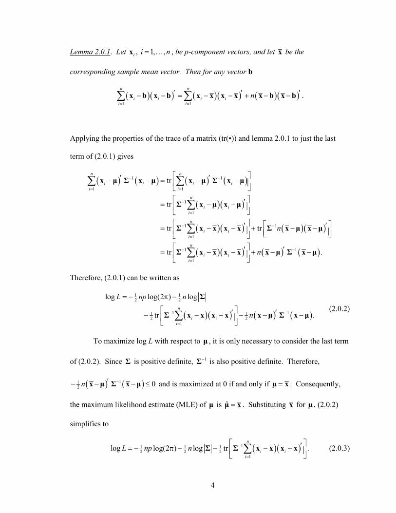
2.6 FACTOR ANALYSIS / STRUCTURAL EQUATION MODELING

Factor analysis is a multivariate procedure in which one tries to account for the

covariances among the observed variables by a smaller number of underlying

22

hypothetical variables, called factors. Let ix , 1, ,i n= K , be p-component vectors of

observations from a population with mean µ and covariance matrix Σ . The factor

analysis model is given by i = + +x µ Λf e , where f is an 1m× ( m p< ) vector of

underlying factors, Λ is a p m× matrix of factor loadings, and e is a 1p× vector of

residuals. It is assumed that the underlying factors are independently and identically

distributed with mean 0 and covariance matrix I, that the residuals are independently

distributed with mean 0 and covariance matrix Ψ , and that f and e are independent.

Therefore,

Cov( ) Cov( )Cov( ) Cov( )

i = + +

= +′= +

′= +

x µ Λf eΛf e

ΛIΛ ΨΛΛ Ψ

In most applications, factor analysis is performed on the centered data, i −x µ , since

Cov( ) Cov( )i i− =x µ x . Therefore, for the remainder of this section, the p-component

vector ix will represent the centered data.

In factor analysis, the researcher hypothesizes an adequate number of underlying

factors, then chooses one of many methods to estimate Λ , based on the chosen number

of factors. One such method of estimation is the maximum likelihood method. The

advantage of using this procedure is, assuming the data come from a multivariate normal

population, that it allows the computation of a likelihood ratio test statistic that can be

used to test the goodness of fit of the chosen number of factors. This is a test of 0H :

there are m underlying factors, or in matrix form, 0 : FH ′= +Σ ΛΛ Ψ . The details of the

23

derivation of this likelihood ratio test statistic can be found in Lawley & Maxwell (1971).

Briefly, consider the likelihood ratio criterion given by

( )( )

( ) ( )( ){ }( ) ( ){ }

( )( ){ }{ }

122 12

, ,22 11

, 2

1212

212

ˆ ˆ ˆ ˆ ˆ ˆˆ2 exp trmax ,

max , ˆ ˆ ˆ2 exp tr

ˆ ˆ ˆ ˆ ˆ ˆˆexp tr

ˆ exp

nnp

F

F nnp

n

n

nL

L n

n

np

−−−

−− −

−−

−

′ ′π + − +λ = =

π −

′ ′+ − +=

−

µ Λ Ψ

µ Σ

ΛΛ Ψ Σ ΛΛ Ψµ Σ

µ Σ Σ ΣΣ

ΛΛ Ψ Σ ΛΛ Ψ

Σ

where ˆ ˆ,Λ Ψ , and Σ̂ are the MLE’s of ,Λ Ψ , and Σ , respectively. The MLE of Σ can

be found as shown at the beginning of Chapter 2. Namely,

( )( )1

1ˆn

i iin =

′= − −∑Σ x x x x .

Typically, the MLE’s of andΛ Ψ are derived by maximizing the log-likelihood function

with respect to Λ and Ψ . However, Lawley and Maxwell (1971) state that it is more

convenient to minimize

( )( )1*2 log log tr logF n p− ′ ′− λ = + + + − −

ΛΛ Ψ S ΛΛ Ψ S

where the * indicates that the unbiased sample covariance matrix, S, is used in place of

Σ̂ in Fλ . Minimizing *2 log F− λ instead of maximizing

( )( )11 1 12 2 2

ˆlog log(2 ) log trFL np n n −′ ′= − π − + − +ΛΛ Ψ Σ ΛΛ Ψ

is acceptable since they differ by a constant, 12 log(2 )np− π , and a function of the data,

log p− −S , and the remaining terms of log FL are just 1 2− times the corresponding

terms of *2 log F− λ . The only other difference between log FL and *2 log F− λ is in the use

24

of S in *2 log F− λ rather than Σ̂ . Since 1ˆn

n−=S Σ , these matrices will be essentially

equivalent for large n.

To find Λ̂ and Ψ̂ let ijσ and ijλ be the elements in the ith row and jth column of

Σ and Λ , respectively. Also, let iψ be the ith diagonal element of Ψ . (The non-

diagonal elements of Ψ are all zero, since the residuals are independently distributed.)

Then,

2

1

m

ii ik ik=

σ = λ +ψ∑ and 1

,m

ij ik jkk

i j=

σ = λ λ ≠∑ ,

and the MLE’s of Λ and Ψ can be found by setting the following expressions equal to

zero and solving simultaneously for ijλ and iψ ;

1

log log log logandp

ij iiF F F F

jil ij il i ii i

L L L L=

∂σ ∂σ∂ ∂ ∂ ∂= ⋅ = ⋅ ∂λ ∂σ ∂λ ∂ψ ∂σ ∂ψ ∑ .

In most cases, these equations cannot be solved directly. Therefore, an iterative

numerical procedure, such as Newton-Raphson, scoring, or steepest descent must be used

to find the MLE’s.

To perform this likelihood ratio test, we must know how the test statistic is

distributed. Lawley and Maxwell (1971) found that *2 log F− λ is asymptotically

distributed as a chi-squared random variable with ( ) ( )212 p m p m − − + degrees of

freedom. For many years, this likelihood ratio test was the primary criterion used to

determine the goodness of fit of the hypothesized number of factors. However, in the

early 1980’s researchers discovered through Monte Carlo simulation that in large

25

samples, good-fitting models were rejected too often, and in small samples the type I

error rates were too large and power was very poor (Gerbing & Anderson, 1993).

26

CHAPTER 3

BOOTSTRAPPING

At least one non-parametric procedure has been applied to the problem of testing

the structure of a covariance matrix. Specifically, bootstrapping has been used to

estimate the distribution of the likelihood ratio test statistic used in structural equation

modeling. Consider testing the hypothesis 0 : ( )H =Σ Σ θ , where ( )Σ θ is the

hypothesized covariance structure expressed as a function of the vector of parameters, θ .

To perform a bootstrap test, the resampling must be done from a bootstrap population

with covariance structure specified by the null hypothesis. Therefore, the observed data

must be transformed as follows before resampling (Bollen & Stine, 1993). Let X be the

n p× matrix of centered data, let /( 1)n′= −S X X denote the sample covariance matrix of

X, and let ( )ˆˆ =Σ Σ θ be the estimated hypothesized covariance structure. Also, let 1 2M

denote the lower triangular matrix resulting from the Cholesky decomposition of a

positive definite matrix M. Then, the sample covariance matrix of 1 2 1 2ˆ−=Y XS Σ is

given by

27

( ) ( )

( ) ( )

( ) ( ) ( )

1 2 1 2 1 2 1 21 11 1

1 2 1 2 1 2 1 2

1 2 1 2 1 2 1 2 1 2 1 2

1 2 1 2

ˆ ˆ

ˆ ˆ

ˆ ˆ

ˆ ˆ

ˆ .

n n− −

− −

− −

− −

′ ′′ ′=

′ ′=

′ ′ ′=

=

=

Y Y Σ S X XS Σ

Σ S SS Σ

Σ S S S S Σ

Σ Σ

Σ

Therefore, the transformed data matrix, Y, has sample covariance structure Σ̂ .

To find the bootstrap distribution of the likelihood ratio test statistic, resample the

rows of the transformed data matrix, Y, with replacement, compute the sample

covariance matrix *S of the resampled data, find the MLE’s of the parameters based on

the resampled data, and compute the likelihood ratio test statistic for the resampled data.

When the null hypothesis is true, the bootstrap distribution is approximately the same as

the distribution of the likelihood ratio test statistic, and a p-value can be computed by

dividing the number of bootstrap samples resulting in a test statistic value at least as large

as the one resulting from the observed data by the total number of bootstrap samples.

28

CHAPTER 4

PERMUTATION TESTS

Permutation tests have long been studied as alternatives to parametric procedures

when the assumptions of such procedures are violated. The idea behind permutation tests

is to generate the sampling distribution of a test statistic from the values obtained by

calculating the test statistic for all possible permutations of the data under the null

hypothesis. Consider a simple example given by Edgington (1995). Suppose five

subjects are randomly assigned to two treatments, A and B, with the following results.

A: 18, 30, 54 B: 6, 12

We wish to test the null hypothesis of no difference in the treatment means. Assuming

this null hypothesis is true, we would expect each subject to have the same result

regardless of their treatment assignment. Therefore, under the null hypothesis, there are

5 3 10C = possible arrangements of subjects to treatments, where n kC is the number of

combinations of k items chosen from a total of n items. These arrangements, as well as

the corresponding test statistic values, are displayed in Table 4.0.1. In this example, the

test statistic is the absolute value of the pooled t-test statistic (displayed as t in Table

4.0.1).

29

Table 4.0.1. All Possible Permutations of the Observed Data

Trt A Trt B t18, 30, 54 6, 12 1.81 6, 12, 18 30, 54 3.00 6, 12, 30 18, 54 1.22 6, 12, 54 18, 30 0.00 6, 18, 30 12, 54 0.83 6, 18, 54 12, 30 0.25 6, 30, 54 12, 18 0.83 12, 18, 30 6, 54 0.52 12, 18, 54 6, 30 0.52 12, 30, 54 6, 18 1.22

The distribution of the test statistic values calculated from each possible

permutation of the data is the sampling distribution of the test statistic. Consequently, a

p-value can be found by dividing the number of observations greater than or equal to the

test statistic value obtained from the observed data, by the total number of permutations

of the data under the null hypothesis. In this example, the p-value is 2 /10 0.20= since

there are two values of t that are greater than or equal to 1.81 (bolded numbers in Table

4.0.1), the value obtained from the observed data. Notice that the 1.81 corresponds to the

most significant data configuration in which the value for treatment A is greater than that

of treatment B and the 3.00 corresponds to the most significant data configuration in

which the value for treatment A is less than that of treatment B. Therefore, a one-tailed

p-value is 1/10 0.10= .

Fisher (1971) is often credited with developing the first permutation tests;

however, Edgington (1995) claims that permutation tests based on the ranks of data have

been used since the 1880’s. Even if Fisher was not the first to develop permutation tests

30

in general, he was the first to suggest permuting the raw data as opposed to the ranks of

the data. He is also responsible for generating considerable interest in the merits of

permutation tests, namely the lack of distributional assumptions required by parametric

tests. Fisher (1971) writes, “The utility of such non-parametric (permutation) tests

consists in their being able to supply confirmation whenever, rightly or, more often,

wrongly, it is suspected that the simpler (parametric) tests have been appreciably injured

by departures from normality” (p. 48). Fisher (1936) even goes on to write in a later

article that conclusions from parametric tests “have no justification beyond the fact that

they agree with those which could have been arrived at by this elementary method

(permutation tests)” (p. 59).

Although Fisher (1971) showed that permutation tests eliminate the need for

normality, it was another statistician, Pitman (1937a, 1937b, 1938), who recognized that

permutation tests also eliminate the need for random samples. In these three papers,

Pitman developed much of the theory of permutation tests and showed that random

sampling is not necessary for a valid test. Rather, random assignment of experimental

units to treatments is sufficient.

Given the benefits of permutation tests, one would assume that the majority of

analyses would be performed utilizing these procedures. However, the ability to

determine the test statistic value for all possible permutations of the observed data was

virtually impossible (except for the smallest sample sizes) due to the lack of computer

technology in Fisher’s and Pitman’s day. Consequently, permutation tests based on ranks

continued to be developed, since these tests do not require the generation of a new

31

sampling distribution for each new set of observed data. Tables exhibiting critical values

were readily available for such tests.

It took significant improvements in technology before interest in permutation tests

based on raw data was renewed; however, the computing time required to generate all

possible permutations of the data was, and still is, prohibitive except for the smallest

sample sizes. Finally, in 1957, Dwass proposed “the almost obvious procedure of

examining a ‘random sample’ of permutations and making the decision to accept or reject

(the null hypothesis) on the basis of those permutations only” (p. 182). He called this

new class of tests randomization tests and found that the power of these tests is ‘close’ to

the power of the corresponding permutation tests. In his 1957 paper, Dwass restricts

attention to the two sample case, but indicates that these randomization tests can be

applied in more general situations.

In more recent years, Edgington (1995), Manly (1997), and Good (1994) have

applied permutation and randomization tests to factorial designs, randomized block

designs, and multivariate designs, among others. Several statisticians have even used

permutation tests to test the equality of correlation or covariance matrices from multiple

populations (Krzanowski, 1993; Shipley, 2000; Zhu, Ng, & Jing, 2003). However,

neither permutation nor randomization tests have been applied to testing the structure of a

covariance matrix.

As a side note, permutation tests are very similar to bootstrapping described in

Chapter 3. The primary difference is that in bootstrapping the resampling is done with

replacement, whereas in permutation tests the resampling is done without replacement.

Because of this, permutation tests are exact and unbiased, whereas Good (1994) writes,

32

“The bootstrap is neither exact nor conservative. Generally, but not

always, a nonparametric bootstrap is less powerful than a permutation

test… If the observations are independent and from distributions with

identical values of the parameter of interest, then the bootstrap is

asymptotically exact” (p. 20).

33

CHAPTER 5

PROPOSED TEST

Recognizing the benefits of permutation tests and the limitations of parametric

procedures for testing the structure of a covariance matrix, it is the purpose of this

research to develop a permutation test for the structure of a covariance matrix. To

develop such a test, it must be established that the observations are exchangeable under

the null hypothesis. Good (2002) gives a simple definition of exchangeability. He writes

that observations are considered exchangeable if, “under the (null) hypothesis, the joint

distribution of the observations is invariant under permutations of the subscripts” (p.

243). He then goes on to say

“It is easy to see that a set of i.i.d. variables is exchangeable. Or that the

joint distribution of a set of normally distributed random variables whose

covariance matrix is such that all diagonal elements have the same value

2σ and all of the off-diagonal elements have the same value ρ is invariant

under permutations of the variable subscripts” (p. 244).

Good (2002) focuses on permuting variable subscripts rather than the actual observations

so as to include permutation tests in which residuals are permuted, but these conditions

for exchangeability also apply to cases in which the raw data are permuted. It will be

argued in the following sections that all of the proposed permutation tests satisfy at least

one of the criteria for exchangeability given by Good.

34

Before describing the permutation tests for the structure of a covariance matrix,

note that covariance matrices are invariant to changes in location. Therefore, it will be

assumed throughout this chapter that the variable means are all equal. If the variable

means are unequal or it is unknown whether the means are equal, the raw data can easily

be centered by calculating i −x µ or i −x x depending on whether µ is assumed known

or unknown, respectively. This centering is necessary to eliminate the effect of the mean

vector when permuting the data. For example, consider a situation in which two

variables are assumed to have equal variances, but one has a mean of 100 and the other a

mean of 1. If the values were permuted between the variables, the assumption of equal

variances would be violated since the relatively ‘large’ values of the first variable would

be combined with the relatively ‘small’ values of the second. This problem, however,

can be remedied without affecting the variance or covariance assumptions by centering

the raw data as described above.

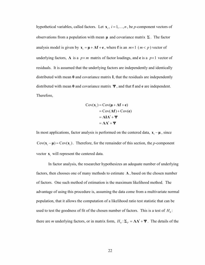
5.1 PERMUTATION TESTS OF SPHERICITY AND COMPOUND SYMMETRY

Consider first a permutation test for compound symmetry. Let ix , 1, ,i n= K , be

equally distributed, p-variate vectors of observations taken on n subjects. We wish to test

:o CSH =Σ Σ where Σ is the covariance matrix of the distribution of ix ,

( )2 1CS p p p′ = σ −ρ +ρ Σ I 1 1 , (5.1.1)

2σ is the common population variance, ρ is the common pairwise correlation, pI is the

p p× identity matrix, and p1 is a 1p× vector of ones. Under the null hypothesis, the

variances are assumed equal and the pairwise correlations are assumed equal, but no

35

distributional assumptions have been made. To completely satisfy one of the conditions

for exchangeability given previously, we would also need to assume joint normality.

However, the simulation results shown in Chapter 6 indicate that this assumption might

be too strict. It does not appear necessary to assume joint normality, but rather that each

of the marginal distributions is from the same family of distributions, i.e. all uniform, all

exponential, etc. Consequently, the values within each vector ix can be permuted

without altering the covariance matrix.

Before developing a test statistic, it is necessary to discuss the estimation of 2σ

and ρ . Consider using the MLEs. Call these 2 211

pjp j

s s=

= ∑ and

( )12

111 1 1

p pjkp p j k j

r r−

− = = += ∑ ∑ , where 2

js and jkr are the usual MLEs of 2jσ and jkρ ,

respectively. Since covariance matrices are symmetric, one possible test statistic can be

computed by summing the absolute differences between the elements on or above the

diagonal of the covariance matrices obtained from each possible permutation and the

elements on or above the diagonal of the covariance matrix estimated as described above.

In matrix notation this test statistic can be expressed as

( ) ( )( )12

21 vec 1perm p p pp pD s r r+

′ ′ = − − + 1 Σ I 1 1

where permΣ is the covariance matrix obtained after permuting the data and vec(M) is a

vector of the elements on or above the diagonal of a matrix M. This test statistic is

computed for each possible permutation of the data and the proportion of test statistic

values greater than or equal to the one obtained from the observed data is the

corresponding p-value. This test for compound symmetry can also be used to test for

sphericity by setting 0r = .

36

Consider a very simple example of the proposed permutation test in which there

are three measurements taken on each of three subjects resulting in the data and sample

statistics shown in Table 5.1.1 below. We are interested in testing whether the

covariance matrix has the compound symmetry structure. This is equivalent to testing

:o CSH =Σ Σ versus :a CSH =/Σ Σ , where CSΣ is of the form of (5.1.1) and 2s and r are

the MLEs of 2σ and ρ given by

( )2 21 131

1.416 1.389 0.436 1.080pjp j

s s=

= ≈ + + ≈∑

and

( ) ( )12

11 131 1 1

0.69 0.99 0.79 0.823p pjkp p j k j

r r−

− = = += ≈ + + ≈∑ ∑ .

In this case, since µ is unknown, the data will be centered by subtracting i −x x for each

subject, i. This results in the centered data shown in Table 5.1.1. Notice that the sample

variances and correlations are invariant to centering.

Table 5.1.1. Observed Data

Raw Data Centered Data 6.4 4.8 1.8 1.17 1.67 0.73 3.6 2.3 0.2 -1.63 -0.83 -0.87 5.7 2.3 1.2 0.47 -0.83 0.13

1 5.23x = 2 3.13x = 3 1.07x = 1 0x = 2 0x = 3 0x =21 1.416s = 2

2 1.389s = 23 0.436s = 2

1 1.416s = 22 1.389s = 2

3 0.436s =

1 0.69 0.990.69 1 0.790.99 0.79 1

R =

1 0.69 0.990.69 1 0.790.99 0.79 1

R =

37

In this example, there are ! 3! 6p = = possible permutations of each row, resulting

in ( ) 3! 6 216np = = possible permutations of the observed data. Four of these

permutations along with the corresponding test statistic values, D, are displayed in Table

5.1.2 below. The bolded data shown in Table 5.1.2 are the observed data.

Table 5.1.2. Some Permutations of the Centered Observed Data

1.17 1.67 0.73 0.73 1.67 1.17 -1.63 -0.83 -0.87 -1.63 -0.87 -0.83 0.47 -0.83 0.13 0.47 -0.83 0.13

= 1.761422D 1.064711D =1.17 0.73 1.67 1.17 1.67 0.73 -0.83 -0.87 -1.63 -0.87 -1.63 -0.83 0.13 0.47 -0.83 0.47 0.13 -0.83

2.587289D = 2.345689D =

The p-value can be found by computing the proportion of test statistic values that

are greater than or equal to the one obtained from the observed data. The distribution of

the test statistic values is shown in Figure 5.1.1. The vertical line at 1.761422 represents

the value of the test statistic resulting from the observed data. In this example, 96 of the

216 possible permutations result in test statistic values greater than or equal to 1.761422.

Therefore, the p-value is 96 / 216 0.4444≈ and at any reasonable type I error rate there is

not enough evidence to conclude that the covariance matrix does not have the compound

symmetry structure.

38

Figure 5.1.1. Distribution of the Test Statistic for Compound Symmetry

Test Statistic

Rel

ativ

eFr

eque

ncy

0.5 1.0 1.5 2.0 2.5

0.0

0.2

0.4

0.6

0.8

5.2 PERMUTATION TEST OF TYPE H STRUCTURE

The type H covariance structure does not satisfy either of the criteria for

exchangeability mentioned previously. Therefore, the transformation described in

Section 2.3 can be applied to the data so that the permutation test for sphericity described

in Section 5.1 can be used. Specifically, assume we wish to test 0 : THH =Σ Σ versus

:a THH ≠Σ Σ , where THΣ has the form of (2.3.1). Let C be a ( )1p p− × matrix of

39

normalized orthogonal contrasts on the p repeated measures and let Y be an n p× matrix

of centered data. Under 0H , ( ) ( ) 1Var ' Var ' 'TH p−= = = γYC C Y C CΣ C I as shown in

Section 2.3. Therefore, the permutation test for sphericity can be applied to the

transformed data, 'YC .

As an example, return to the sample given in Table 5.1.1. This time we wish to

test 0 : THH =Σ Σ . The matrix of normalized orthogonal contrasts is given by

0.7071068 0.7071068 00.4082483 0.4082483 0.8164966

− = − −

C .

Post-multiplying the centered data shown in Table 5.1.1 by 'C yields

1.17 1.67 0.73 0.7071 0.40821.63 0.83 0.87 0.7071 0.4082

0.47 0.83 0.13 0 0.8165

0.3536 0.56340.5657 0.2939 .0.9192 0.2531

− − = − − − ⋅ − −

− = −

YC'

(5.2.1)

The MLE of the covariance matrix of this transformed data is then given by

0.4300 0.08850.0885 0.1559

− −

and the MLE of 1p−γI is given by

�1

0.29295 00 0.29295p−

γ =

I .

The permutation test for sphericity is applied to the transformed data to test

0 1: ' pH −= γCΣC I versus 1: 'a pH −≠ γCΣC I by finding all possible within row

permutations of the transformed data. The test statistic is then calculated by

40

( ) ( )12 1

ˆvec perm pp pD +′= − γ1 Σ I .

A p-value can be found by determining the proportion of test statistic values greater than

or equal to the one resulting from the original set of transformed data. For the

transformed data shown in (5.2.1), there are only ( ) 3! 2 8np = = possible permutations of

which all 8 result in test statistic values greater than or equal to 0.3626011, the test

statistic value resulting from the original set of transformed data. Therefore, the p-value

is 8 /8 1= and at any reasonable type I error rate there is not enough evidence to conclude

that the covariance matrix does not have the type H structure.

One drawback with this permutation test is that the transformed data matrix has

only p-1 as opposed to p columns as in the original data matrix. For large combinations

of n and p this is not a problem. However, if the combination of n and p is small, as in

the example shown above, there may be too few possible permutations for the

permutation test to be meaningful or even useful at all.

5.3 PERMUTATION TEST OF ALL OTHER COVARIANCE STRUCTURES

Neither of the remaining covariance structures discussed in Chapter 2 (serial

correlation and independence of sets of variates) satisfy either of the conditions for

exchangeability described previously. Therefore, a data transformation is required to

achieve exchangeability. The following theorem given by Graybill (1983), can be used

to transform a data set with covariance matrix Σ to one with covariance matrix D, where

D is a diagonal matrix. Finally, one additional calculation, described in the following

paragraphs, enables any test of the structure of a covariance matrix to be accomplished by

a test for sphericity.

41

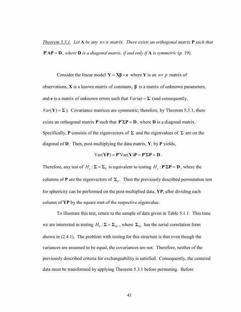
Theorem 5.3.1. Let A be any n n× matrix. There exists an orthogonal matrix P such that

′ =P AP D , where D is a diagonal matrix, if and only if A is symmetric (p. 19).

Consider the linear model = +Y Xβ e where Y is an n p× matrix of

observations, X is a known matrix of constants, β is a matrix of unknown parameters,

and e is a matrix of unknown errors such that ( )Var =e Σ (and consequently,

( )Var =Y Σ ). Covariance matrices are symmetric; therefore, by Theorem 5.3.1, there

exists an orthogonal matrix P such that ′ =P ΣP D , where D is a diagonal matrix.

Specifically, P consists of the eigenvectors of Σ and the eigenvalues of Σ are on the

diagonal of D. Then, post-multiplying the data matrix, Y, by P yields,

Var( ) Var( )′ ′= = =YP P Y P P ΣP D .

Therefore, any test of 0:oH =Σ Σ is equivalent to testing :oH ′ =P ΣP D , where the

columns of P are the eigenvectors of 0Σ . Then the previously described permutation test

for sphericity can be performed on the post-multiplied data, YP, after dividing each

column of YP by the square root of the respective eigenvalue.

To illustrate this test, return to the sample of data given in Table 5.1.1. This time

we are interested in testing 0 : SCH =Σ Σ , where SCΣ has the serial correlation form

shown in (2.4.1). The problem with testing for this structure is that even though the

variances are assumed to be equal, the covariances are not. Therefore, neither of the

previously described criteria for exchangeability is satisfied. Consequently, the centered

data must be transformed by applying Theorem 5.3.1 before permuting. Before

42

transforming the data, consider the following preliminary calculations used to find the

MLEs of 2σ and ρ in SCΣ as described in Section 2.4.

( ) ( )1 114.166667

=′= − − =∑n

i iiS x x C x x ,

( ) ( )2 219.5

=′= − − =∑n

i iiS x x C x x ,

and

( ) ( )3 19.72

=′= − − =∑n

i iiS x x x x

where 1C and 2C are as shown in (2.4.3). Then, the MLE of ρ can be found by

substituting 1S , 2S , 3S , and 3p = into (2.4.5) to get

3 2ˆ ˆ ˆ16.666668 9.5 44.440002 28.5 0ρ − ρ − ρ+ = .

The only solution to this equation in the interval (-1, 1) is ρ̂ 0.6549899= . Substituting

this value into (2.4.4) yields 2ˆ 0.5872383σ = . Therefore, under the null hypothesis the

MLE of the covariance matrix is

1.0284596 0.6736306 0.4412212ˆ 0.6736306 1.0284596 0.6736306

0.4412212 0.6736306 1.0284596SC

=

Σ

and the eigenvectors and eigenvalues of ˆSCΣ are

17

0.5535 0.7071 0.44000.6223 5.4400 10 0.78280.5535 0.7071 0.4400

−

× − −

and [ ]2.2269 0.5872 0.2712 ,

respectively. Post-multiplying the centered data matrix shown in Table 5.1.1 by the

matrix of eigenvectors yields

43

17

1.17 1.67 0.73 0.5535 0.7071 0.44001.63 0.83 0.87 0.6223 5.4400 10 0.7828

0.47 0.83 0.13 0.5535 0.7071 0.4400

2.0888 0.3064 0.46871.9024 0.5421 0.4477 ;0.1864 0.2357 0.9163

−

− − − ⋅ × − − −

− = − − − −

(5.3.1)

however, this data matrix still cannot be permuted since the variances of the variables,

given by the eigenvalues, are not equivalent. Therefore, each column of this data matrix

must be divided by the square root of its respective eigenvalue before the data can be

permuted. Refer to the data matrix found by dividing each column of (5.3.1) by the

square root of its respective eigenvalue. We will refer to this matrix as the matrix of

transformed data. This matrix is given by

1.3997 0.3999 0.90001.2748 0.7074 0.85960.1249 0.3076 1.7596

− − − − −

. (5.3.2)

We can now perform a test for sphericity on the matrix of transformed data. This

is done by finding all possible permutations of the transformed data such that the data are

permuted within each row, and calculating the test statistic given by

( ) ( )12 1 vec perm pp pD +′= −1 Σ I .

A p-value can be found by determining the proportion of test statistic values greater than

or equal to the one resulting from the original set of transformed data. For the

transformed data shown in (5.3.2), there are ( ) 3! 6 216np = = possible permutations of

which only 6 result in test statistic values greater than or equal to 0.6095927 which is the

value resulting from the original set of transformed data. Therefore, the p-value is

6 / 216 0.0278≈ and at α 0.05= there is enough evidence to conclude that Σ does not

44

have the serial correlation structure. This conclusion is expected since the sample

correlation matrix shown in Table 5.1.1 does not suggest serial correlation. Figure 5.3.1

below shows the distribution of the test statistic for this set of data. The vertical line at

0.6095927 represents the test statistic value resulting from the original set of transformed

data.

Figure 5.3.1. Distribution of the Test Statistic for Serial Correlation

Test Statistic

Rel

ativ

eFr

eque

ncy

0.0 0.1 0.2 0.3 0.4 0.5 0.6

0.0

0.5

1.0

1.5

2.0

2.5

3.0

45

CHAPTER 6

SIMULATIONS

One-thousand simulations were run using R version 2.3.1 for all combinations of

n ( 5,10,25= ) and p ( 3,5,10= ). The R code for each test can be found in Appendix A.1.

Due to the extremely large number of permutations required to perform the permutation

tests described in Chapter 5 for any reasonable values of n and p, randomization tests

were primarily used in the simulations. Permutation tests were only run for the test of

type H structure when 5n = or 10 and 3p = (see Section 6.3). Within each simulation,

a p-variate data set was generated and the randomization test (RT) (or permutation test

[PT] in the cases described above), likelihood ratio test (LRT), and corrected likelihood

ratio test (CLRT) were all run for comparison. One-thousand random permutations of the

centered and/or transformed data were sampled for each RT. The number of randomly

selected permutations was chosen according to the suggestions of Manly (1997). For the

LRTs, the asymptotic chi-squared distributions described in Chapter 2 were used to

determine approximate 5% critical values.

Three different multivariate distributions (normal, uniform, and double

exponential) were investigated. For the multivariate normal distribution, data were

generated using the built-in R functions by specifying the desired covariance structure.

For the multivariate double exponential distributions data were generated using a

46

procedure described in Vale and Maurelli (1983). For univariate data, this procedure first

involves the generation of a random sample from a standard normal distribution. Each of

these data values, X, is then substituted into the polynomial 2 3Y a bX cX dX= + + + ,

where the constants a, b, c, and d are determined by expressing the first four moments of

the desired non-normal distribution in terms of the first four moments of the standard

normal distribution and solving algebraically. Vale and Maurelli (1983) provide a system

of equations that can be used to find these constants. In extending this to the multivariate

case, there are issues with specifying the desired covariance structure. Initially, data can

be generated from the ( ),pN 0 Σ distribution, however, once the polynomial

transformation is applied, the resulting data no longer have the same covariance structure.

Therefore, it is necessary to determine intermediate correlations to be used to generate the

multivariate normal data that will result in multivariate double exponential data with the

desired covariance structure. Again, Vale and Maurelli (1983) provide a system of

equations that can be solved to determine these intermediate correlations.

There exists a more recent extension of the Vale and Maurelli (1983) procedure

developed by Headrick (2002) in which the first six moments of the desired non-normal

distribution are used instead of just the first four. Headrick (2002) argues that specifying

two additional moments results in much more accurate non-normal distributions, but the

inclusion of these additional moments places restrictions on the possible correlations that

can be simulated. Specifically, once one of the correlations in the desired covariance

matrix is specified, the remaining correlations cannot differ from the first too drastically,

and the amount of difference changes for each desired distribution. For example, in

trying to simulate three-variate uniform data with an unstructured covariance matrix, the

47

largest and smallest of the three correlations could not be varied by more than

approximately 0.3. Differences larger than this resulted in intermediate correlations that

were greater than one. This restriction is not a problem when generating data with a

compound symmetry covariance structure; however, it severely limits the number of

alternative covariance structures that can be explored when estimating power, especially

as the number of variables is increased. Therefore, the method given by Vale and

Maurelli (1983) was used to generate the multivariate double exponential data for the

simulations in this chapter.

Although convenient for generating data from many multivariate distributions, the

Vale and Maurelli (1983) procedure cannot be used to generate multivariate uniform

data. This is due to the fact that this procedure restricts the lower bound of the kurtosis of

the desired marginal distributions. Specifically, if the skewness of the desired marginal

distribution is 0, the lower bound for kurtosis is -1.15132 (Headrick, 2002); whereas the

kurtosis of the UNIF(a,b) distribution is -1.2. Therefore, to generate the multivariate

uniform data, a procedure described in Falk (1999) was used. This procedure consists of

generating a random sample, ix , 1,...i n= , from the ( ),pN 0 R% distribution where

( )62sin π=R R% and R is the desired correlation matrix. Then the standard normal CDF,

Φ , is applied to the ( ),pN 0 R% data so that ( )iΦ x has a multivariate ( )UNIF ,p p0 1

distribution with correlation matrix R, where p0 and p1 are 1p× vectors of zeros and

ones, respectively, that represent the lower and upper bounds of the marginal uniform

distributions. To achieve the desired variances, note that the variance of the univariate

UNIF(a,b) distribution is given by ( )22 12b aσ = − . Setting 0a = we have 2 2 12bσ =

48

which implies that 12b = σ . Multiplying each column of the multivariate

( )UNIF ,p p0 1 data by 12j jjb = σ , 1,...,j p= , with the desired standard deviation, jjσ ,

results in multivariate ( )UNIF ,p0 b data with covariance matrix Σ , where

( )1,..., 'pb b=b .

The type I error rate and power will be investigated for five different

randomization tests: the tests of sphericity, compound symmetry, type H, serial

correlation, and independence of sets of variates. The tests of sphericity and compound

symmetry will be performed by permuting the raw data; the test of type H structure will

be performed by first post-multiplying the data matrix by a matrix of normalized

orthogonal contrasts and then running the randomization test for sphericity; and the tests

of serial correlation and independence of sets of variates will be performed by first post-

multiplying the data matrix by the eigenvectors of the estimated hypothesized covariance

matrix, then dividing the columns of the resulting matrix by the square root of the

respective eigenvalues, and finally running the randomization test for sphericity.

The values of the various parameters used to simulate the type I error rates for the

different tests are as follows. For sphericity, the covariance structure is given by

2S p= σΣ I where 2σ =1, 9, or 25; for Compound Symmetry, the covariance structure is

given by

( )2 1CS p p p′ = σ −ρ +ρ Σ I 1 1 (6.0.1)

where 2σ =1, 9, or 25 and ρ = 0.3, 0.6, or 0.9; for Type H, the covariance structure is

given by

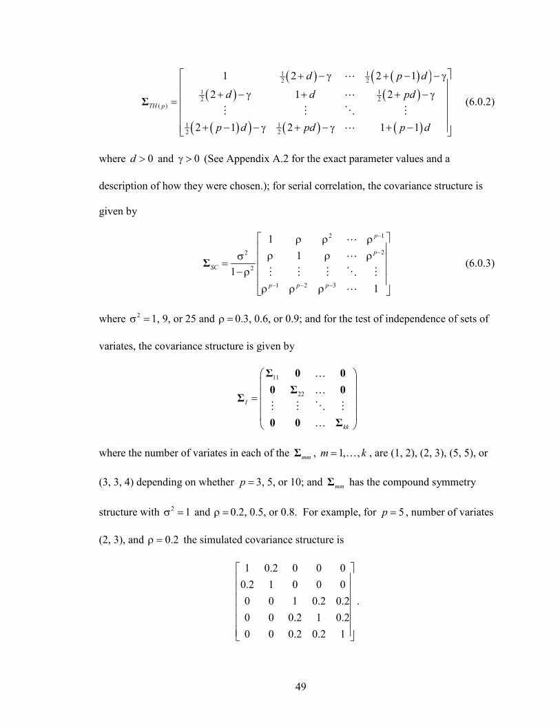
49

( ) ( )( )( ) ( )

( )( ) ( ) ( )

1 12 2

1 12 2

( )

1 12 2

1 2 2 1

2 1 2

2 1 2 1 1

TH p

d p d

d d pd

p d pd p d

+ − γ + − − γ

+ − γ + + − γ =

+ − − γ + − γ + −

Σ

L

L

M M O M

L

(6.0.2)

where 0d > and 0γ > (See Appendix A.2 for the exact parameter values and a

description of how they were chosen.); for serial correlation, the covariance structure is

given by

2 1

22

2

1 2 3

11

11

p

p

SC

p p p

−

−

− − −

ρ ρ ρ ρ ρ ρσ = −ρ ρ ρ ρ

Σ

L

L

M M M O M

L

(6.0.3)

where 2σ =1, 9, or 25 and ρ = 0.3, 0.6, or 0.9; and for the test of independence of sets of

variates, the covariance structure is given by

11

22I

kk

=

Σ 0 00 Σ 0

Σ

0 0 Σ

K

K

M M O M

K

where the number of variates in each of the mmΣ , 1, ,m k= K , are (1, 2), (2, 3), (5, 5), or

(3, 3, 4) depending on whether p = 3, 5, or 10; and mmΣ has the compound symmetry

structure with 2 1σ = and ρ = 0.2, 0.5, or 0.8. For example, for 5p = , number of variates

(2, 3), and 0.2ρ = the simulated covariance structure is

1 0.2 0 0 00.2 1 0 0 00 0 1 0.2 0.20 0 0.2 1 0.20 0 0.2 0.2 1

.

50

The various covariance structures used to investigate power are detailed in the

sections to follow.

6.1 TEST OF SPHERICITY

Simulated type I error rates for the test of sphericity are displayed in Table 6.1.1.

For normally distributed data, the CLRT performs better than the other two tests with

respect to the simulated type I error rates. For uniform data, the CLRT underestimates

the nominal type I error rate and for double exponential data the CLRT overestimates the

nominal type I error rate. These results are consistent with those of Huynh and

Mandeville (1979) who performed a simulation study of Mauchly’s (1940) test of

sphericity and found that for light-tailed distributions the LRTs were conservative and for

heavy-tailed distributions, the simulated type I error rates exceeded the nominal rate.

This same pattern is slightly seen in the results of the RT, however, the simulated type I

error rates of the RT appear to be converging to 0.05 as n increases, whereas the

simulated type I error rates of the LRTs do not.

The simulated type I error rates for the RT seem to be unaffected by changes in

the variance, however, they appear to increase as p increases. This latter pattern is also

seen in the LRTs, but not as greatly as for the RT. One definite benefit of the RT is that

it is applicable in situations for which the LRTs do not exist, specifically when p n≥ .

However, the simulated type I error rates for these cases are much too large.

Overall, the RT appears to be a viable alternative when the data are not normally

distributed, but it is not beneficial in small sample situations or in cases where n is close

to p. Clearly, the RT is preferred over the LRTs for cases in which p n≥ for the simple

51

fact that a p-value exists for the RT when it does not for the LRTs. However, the

simulated type I error rates are much too large to be of any practical use.

The CLRT does not appear to be a level α test in non-normal situations and

clearly outperforms the LRT. Similarly, the RT does not appear to be a level α test

when p n≥ . Therefore, all three tests will be largely ignored in these situations for the

power discussions to follow. For completeness all three tests were included in the

simulations.

52

Table 6.1.1. Simulated Type I Error Rates for the Test of Sphericity

a. Normal

p=3 p=5 p=10 n σ²=1 σ²=9 σ²=25 σ²=1 σ²=9 σ²=25 σ²=1 σ²=9 σ²=25

RT 0.095 0.079 0.078 0.169 0.175 0.183 0.550 0.553 0.550 LRT 0.303 0.309 0.320 NA NA NA NA NA NA 5

CLRT 0.054* 0.070 0.058* NA NA NA NA NA NA RT 0.070 0.075 0.079 0.100 0.122 0.093 0.204 0.202 0.183

LRT 0.125 0.136 0.138 0.296 0.295 0.317 NA NA NA 10 CLRT 0.043* 0.059* 0.056* 0.051* 0.066 0.071 NA NA NA

RT 0.064 0.053* 0.044* 0.086 0.079 0.075 0.108 0.098 0.100 LRT 0.085 0.078 0.073 0.130 0.091 0.117 0.327 0.317 0.322 25

CLRT 0.062* 0.050* 0.049* 0.058* 0.050* 0.060* 0.079 0.060* 0.069

b. Uniform

p=3 p=5 p=10 n σ²=1 σ²=9 σ²=25 σ²=1 σ²=9 σ²=25 σ²=1 σ²=9 σ²=25

RT 0.095 0.095 0.098 0.166 0.158 0.160 0.449 0.471 0.476 LRT 0.278 0.288 0.277 NA NA NA NA NA NA 5

CLRT 0.054* 0.057* 0.059* NA NA NA NA NA NA RT 0.056* 0.061* 0.067 0.082 0.095 0.088 0.170 0.150 0.146

LRT 0.092 0.075 0.087 0.189 0.204 0.191 NA NA NA 10 CLRT 0.035 0.032 0.021 0.046* 0.043* 0.037* NA NA NA

RT 0.048* 0.056* 0.050* 0.071 0.063* 0.063* 0.077 0.082 0.076 LRT 0.036 0.037* 0.037* 0.061* 0.058* 0.054* 0.202 0.198 0.194 25

CLRT 0.021 0.024 0.025 0.025 0.028 0.020 0.031 0.026 0.019

c. Double Exponential

p=3 p=5 p=10 n σ²=1 σ²=9 σ²=25 σ²=1 σ²=9 σ²=25 σ²=1 σ²=9 σ²=25

RT 0.105 0.120 0.104 0.238 0.212 0.226 0.598 0.613 0.609 LRT 0.422 0.440 0.407 NA NA NA NA NA NA 5

CLRT 0.087 0.126 0.096 NA NA NA NA NA NA RT 0.083 0.081 0.083 0.112 0.122 0.113 0.239 0.238 0.226

LRT 0.262 0.243 0.252 0.470 0.454 0.451 NA NA NA 10 CLRT 0.131 0.126 0.134 0.152 0.148 0.143 NA NA NA

RT 0.062* 0.067 0.064 0.070 0.080 0.072 0.102 0.111 0.103 LRT 0.226 0.223 0.190 0.288 0.305 0.292 0.587 0.604 0.602 25

CLRT 0.169 0.180 0.143 0.183 0.200 0.186 0.239 0.250 0.239 *Value is contained within 0.05 1.96 (0.05)(0.95) /1000±

53

Table 6.1.2 contains the simulated power of the test of sphericity versus non-

homoscedasticity. Specifically, multivariate data were generated from distributions with

covariance matrices having diagonal elements given by 1, 1+d/(p-1), 1+2d/(p-1), …, 1+d

and zero off diagonal elements, where d=4, 8, or 12 represents the difference between the

first and last (or smallest and largest) diagonal elements.

As expected, the power of both the RT and CLRT increases as d and/or n

increases, and the power of both tests decreases as p approaches n. For normally

distributed data the power of the CLRT is greater than that for the RT in most cases, but

the RT does seem to perform fairly well, achieving a power of at least 0.75 for five of the

nine cases when n=25. The true benefit of the RT is seen in the non-normal cases. For

these cases, it appears that the CLRT is outperforming the RT; however, recall from

Table 6.1.1 that there is evidence that neither of the LRTs are α -level tests for non-

normal data. There does appear to be a distributional effect on the simulated power of

the RT with the greatest power resulting from uniformly distributed data and the least

from double exponential data in most cases. For uniform data, the RT achieves a power

of at least 0.75 in all nine of the cases when n=25 and for double exponential data, in one

of the nine cases.

54

Table 6.1.2. Simulated Power vs. Non-Homoscedasticity for the Test of Sphericity

a. Normal

p=3 p=5 p=10 n d=4 d=8 d=12 d=4 d=8 d=12 d=4 d=8 d=12

RT 0.178 0.191 0.217 0.255 0.326 0.313 0.604 0.627 0.622 LRT 0.513 0.614 0.685 NA NA NA NA NA NA 5

CLRT 0.130 0.197 0.236 NA NA NA NA NA NA RT 0.283 0.383 0.426 0.299 0.401 0.384 0.408 0.467 0.470

LRT 0.513 0.778 0.899 0.599 0.803 0.887 NA NA NA 10 CLRT 0.315 0.600 0.746 0.219 0.403 0.532 NA NA NA

RT 0.730 0.915 0.967 0.654 0.803 0.866 0.616 0.749 0.817 LRT 0.873 0.997 1.000 0.834 0.987 0.998 0.932 0.992 0.999 25

CLRT 0.843 0.995 1.000 0.735 0.965 0.996 0.639 0.912 0.988

b. Uniform

p=3 p=5 p=10 n d=4 d=8 d=12 d=4 d=8 d=12 d=4 d=8 d=12

RT 0.195 0.243 0.282 0.299 0.299 0.375 0.580 0.608 0.588 LRT 0.449 0.603 0.689 NA NA NA NA NA NA 5

CLRT 0.091 0.131 0.212 NA NA NA NA NA NA RT 0.433 0.560 0.623 0.401 0.488 0.573 0.433 0.515 0.521

LRT 0.442 0.796 0.932 0.534 0.743 0.874 NA NA NA 10 CLRT 0.212 0.537 0.777 0.145 0.303 0.478 NA NA NA

RT 0.957 0.988 1.000 0.868 0.965 0.989 0.787 0.896 0.920 LRT 0.933 1.000 1.000 0.844 0.997 1.000 0.900 0.997 1.000 25

CLRT 0.892 0.999 1.000 0.713 0.991 1.000 0.532 0.900 0.985

c. Double Exponential

p=3 p=5 p=10 n d=4 d=8 d=12 d=4 d=8 d=12 d=4 d=8 d=12

RT 0.165 0.220 0.244 0.263 0.338 0.320 0.634 0.629 0.614 LRT 0.573 0.657 0.747 NA NA NA NA NA NA 5

CLRT 0.173 0.221 0.297 NA NA NA NA NA NA RT 0.236 0.327 0.360 0.244 0.314 0.344 0.358 0.404 0.421

LRT 0.554 0.777 0.880 0.688 0.823 0.889 NA NA NA 10 CLRT 0.378 0.632 0.761 0.353 0.497 0.638 NA NA NA

RT 0.470 0.665 0.756 0.457 0.601 0.667 0.429 0.578 0.638 LRT 0.843 0.984 0.996 0.858 0.977 0.991 0.945 0.989 0.999 25

CLRT 0.804 0.976 0.995 0.808 0.958 0.983 0.779 0.942 0.978

55

Table 6.1.3 contains the simulated power for the test of sphericity versus non-zero

correlation. Data were generated from multivariate distributions with marginal variances

of 1 and pairwise correlations of ρ = 0.3, 0.6, or 0.9.

As seen in Table 6.1.3, the power of the RT for sphericity versus non-zero

correlation is very low, virtually indistinguishable from the simulated type I error rates

shown in Table 6.1.1. The CLRT, however, has much greater power. For n=10, the

CLRT has power greater than 0.9 when 0.9ρ = and for n=25 when 0.6ρ = or 0.9, but

the CLRT seems to have trouble detecting a correlation of 0.3ρ = even for samples as

large as 25. The simulated power of the CLRT increases as p increases. This pattern is

also evident for the RT, but the increase is not as extreme. The simulated power of the

RT appears to be unaffected by the increase in ρ , whereas the power of the CLRT clearly

increases as ρ increases. Just as in Table 6.1.2, there appears to be a distributional effect

on the simulated power of the RT. However, in Table 6.1.3 the pattern is reversed with

the greatest power resulting from double exponential data and the least from uniform data

in most cases.

56

Table 6.1.3. Simulated Power vs. Non-Zero Correlation for the Test of Sphericity

a. Normal

p=3 p=5 p=10 n ρ=0.3 ρ=0.6 ρ=0.9 ρ=0.3 ρ=0.6 ρ=0.9 ρ=0.3 ρ=0.6 ρ=0.9

RT 0.075 0.044 0.061 0.128 0.093 0.072 0.338 0.156 0.101 LRT 0.402 0.616 0.944 NA NA NA NA NA NA 5

CLRT 0.094 0.185 0.688 NA NA NA NA NA NA RT 0.058 0.042 0.054 0.074 0.050 0.070 0.119 0.043 0.050

LRT 0.288 0.722 0.999 0.540 0.911 1.000 NA NA NA 10 CLRT 0.146 0.553 0.993 0.210 0.750 1.000 NA NA NA

RT 0.039 0.040 0.046 0.045 0.041 0.045 0.054 0.062 0.053 LRT 0.455 0.986 1.000 0.742 1.000 1.000 0.975 1.000 1.000 25

CLRT 0.393 0.980 1.000 0.645 0.999 1.000 0.877 1.000 1.000

b. Uniform

p=3 p=5 p=10 n ρ=0.3 ρ=0.6 ρ=0.9 ρ=0.3 ρ=0.6 ρ=0.9 ρ=0.3 ρ=0.6 ρ=0.9

RT 0.062 0.045 0.057 0.128 0.077 0.077 0.292 0.114 0.086 LRT 0.338 0.590 0.936 NA NA NA NA NA NA 5

CLRT 0.080 0.207 0.696 NA NA NA NA NA NA RT 0.047 0.028 0.059 0.053 0.040 0.059 0.093 0.035 0.029

LRT 0.235 0.706 0.998 0.501 0.903 1.000 NA NA NA 10 CLRT 0.125 0.541 0.996 0.178 0.709 1.000 NA NA NA

RT 0.040 0.042 0.037 0.044 0.041 0.042 0.048 0.028 0.053 LRT 0.392 0.975 1.000 0.714 0.999 1.000 0.960 1.000 1.000 25

CLRT 0.338 0.966 1.000 0.603 0.999 1.000 0.813 1.000 1.000

c. Double Exponential

p=3 p=5 p=10 n ρ=0.3 ρ=0.6 ρ=0.9 ρ=0.3 ρ=0.6 ρ=0.9 ρ=0.3 ρ=0.6 ρ=0.9

RT 0.107 0.064 0.108 0.137 0.107 0.126 0.370 0.208 0.189 LRT 0.501 0.645 0.959 NA NA NA NA NA NA 5

CLRT 0.134 0.243 0.721 NA NA NA NA NA NA RT 0.073 0.063 0.077 0.077 0.061 0.082 0.133 0.074 0.098

LRT 0.397 0.784 0.998 0.673 0.943 1.000 NA NA NA 10 CLRT 0.231 0.619 0.997 0.325 0.795 0.998 NA NA NA

RT 0.055 0.048 0.049 0.057 0.051 0.059 0.067 0.049 0.064 LRT 0.568 0.986 1.000 0.835 0.998 1.000 0.991 1.000 1.000 25

CLRT 0.516 0.981 1.000 0.747 0.997 1.000 0.933 1.000 1.000

57

The simulated power of the test of sphericity versus the type H structure seen in

(6.0.2) is displayed in Tables 6.1.4 through 6.1.6. See Appendix A.2 for a description of

how and why the values of d and γ were chosen.

As expected the power of both the RT and CLRT increases as d and/or n

increases, but there does not appear to be much of a change in the power of the tests as γ

increases. It is difficult to determine the effect of p on the simulated power of the tests

due to the fact that it was necessary to use radically different values of d and γ as p

increased (See Appendix A.2), but there are two cases with equal parameter values.

These are when d=0.1, γ=1, and p=5 (Table 6.1.5) or p=10 (Table 6.1.5). From these two

cases, it appears that the power of both the RT and CLRT increases as p increases. The

CLRT is more powerful than the RT in most cases, but recall that the CLRT is not an α-

level test for non-normal data (See Table 6.1.1). Even with normally distributed data, the

RT appears to have a slight edge over the CLRT with respect to power when d, n, and p

are all small. Overall, the ability of the RT for sphericity to detect the type H structure is

fairly good with simulated power values greater than 0.75 when n=25 in fifteen of the 27

cases for normal data, 21 of the 27 cases for uniform data, and nine of the 27 cases for

double exponential data. Just as in previous tables there appears to be a distributional

effect on the simulated power of the RT, but the pattern is again reversed from that seen

in the previous table (Table 6.1.3) with the greatest power values resulting from uniform

data and the lowest from double exponential data in most cases.

58

Table 6.1.4. Simulated Power vs. Type H for the Test of Sphericity ( 3p = )

a. Normal

γ=2 γ=3 γ=4 n d=1 d=2 d=3 d=2 d=3 d=4 d=3 d=4 d=5

RT 0.153 0.182 0.212 0.240 0.195 0.235 0.292 0.245 0.265 LRT 0.453 0.674 0.904 0.651 0.744 0.923 0.843 0.846 0.975 5

CLRT 0.111 0.241 0.527 0.217 0.255 0.518 0.347 0.366 0.626 RT 0.274 0.419 0.594 0.484 0.565 0.663 0.555 0.694 0.757

LRT 0.437 0.806 0.991 0.800 0.921 1.000 0.982 0.993 1.000 10 CLRT 0.261 0.663 0.975 0.622 0.806 0.992 0.936 0.961 0.999

RT 0.690 0.943 0.993 0.930 0.995 1.000 0.994 1.000 1.000 LRT 0.797 0.996 1.000 0.996 1.000 1.000 1.000 1.000 1.000 25

CLRT 0.741 0.993 1.000 0.994 1.000 1.000 1.000 1.000 1.000

b. Uniform

γ=2 γ=3 γ=4 n d=1 d=2 d=3 d=2 d=3 d=4 d=3 d=4 d=5

RT 0.185 0.204 0.285 0.284 0.260 0.303 0.350 0.308 0.319 LRT 0.438 0.665 0.913 0.641 0.722 0.934 0.851 0.875 0.982 5

CLRT 0.103 0.183 0.511 0.177 0.256 0.504 0.338 0.370 0.681 RT 0.349 0.580 0.803 0.597 0.774 0.859 0.707 0.852 0.911

LRT 0.354 0.804 0.999 0.816 0.939 0.999 0.983 0.995 1.000 10 CLRT 0.180 0.606 0.979 0.616 0.833 0.993 0.940 0.971 1.000

RT 0.894 0.999 1.000 0.998 1.000 1.000 1.000 1.000 1.000 LRT 0.803 0.999 1.000 1.000 1.000 1.000 1.000 1.000 1.000 25

CLRT 0.744 0.998 1.000 1.000 1.000 1.000 1.000 1.000 1.000

c. Double Exponential

γ=2 γ=3 γ=4 n d=1 d=2 d=3 d=2 d=3 d=4 d=3 d=4 d=5

RT 0.162 0.146 0.201 0.255 0.200 0.239 0.282 0.253 0.265 LRT 0.509 0.701 0.924 0.713 0.766 0.932 0.854 0.878 0.973 5

CLRT 0.141 0.262 0.535 0.254 0.353 0.537 0.378 0.430 0.712 RT 0.216 0.332 0.455 0.385 0.441 0.561 0.508 0.561 0.642

LRT 0.500 0.834 0.996 0.812 0.914 0.995 0.980 0.986 1.000 10 CLRT 0.347 0.696 0.988 0.674 0.809 0.984 0.929 0.955 0.999

RT 0.471 0.707 0.907 0.804 0.927 0.939 0.907 0.976 0.980 LRT 0.806 0.996 1.000 0.992 1.000 1.000 1.000 1.000 1.000 25

CLRT 0.766 0.994 1.000 0.991 1.000 1.000 1.000 1.000 1.000

59

Table 6.1.5. Simulated Power vs. Type H for the Test of Sphericity ( 5p = )

a. Normal

γ=1 γ=1.25 γ=1.5 n d=0.1 d=0.4 d=0.8 d=0.1 d=0.5 d=0.9 d=0.2 d=0.6 d=1

RT 0.148 0.161 0.205 0.166 0.216 0.240 0.217 0.222 0.240 LRT NA NA NA NA NA NA NA NA NA 5

CLRT NA NA NA NA NA NA NA NA NA RT 0.110 0.207 0.465 0.140 0.256 0.479 0.185 0.331 0.543

LRT 0.430 0.874 0.999 0.379 0.855 0.996 0.504 0.844 1.000 10 CLRT 0.122 0.615 0.980 0.086 0.553 0.973 0.137 0.549 0.980

RT 0.105 0.524 0.952 0.146 0.664 0.957 0.331 0.823 0.989 LRT 0.416 0.997 1.000 0.211 0.997 1.000 0.631 0.995 1.000 25

CLRT 0.290 0.989 1.000 0.116 0.987 1.000 0.502 0.981 1.000

b. Uniform

γ=1 γ=1.25 γ=1.5 n d=0.1 d=0.4 d=0.8 d=0.1 d=0.5 d=0.9 d=0.2 d=0.6 d=1

RT 0.153 0.162 0.287 0.173 0.201 0.315 0.222 0.233 0.311 LRT NA NA NA NA NA NA NA NA NA 5

CLRT NA NA NA NA NA NA NA NA NA RT 0.100 0.318 0.681 0.138 0.386 0.667 0.211 0.479 0.722

LRT 0.346 0.846 0.998 0.280 0.819 1.000 0.417 0.856 1.000 10 CLRT 0.098 0.581 0.989 0.055 0.517 0.986 0.099 0.522 0.991

RT 0.130 0.865 0.996 0.172 0.940 0.999 0.411 0.987 1.000 LRT 0.307 0.993 1.000 0.119 0.995 1.000 0.516 0.998 1.000 25

CLRT 0.186 0.986 1.000 0.063 0.981 1.000 0.367 0.989 1.000

c. Double Exponential

γ=1 γ=1.25 γ=1.5 n d=0.1 d=0.4 d=0.8 d=0.1 d=0.5 d=0.9 d=0.2 d=0.6 d=1

RT 0.185 0.178 0.225 0.234 0.180 0.245 0.263 0.241 0.271 LRT NA NA NA NA NA NA NA NA NA 5

CLRT NA NA NA NA NA NA NA NA NA RT 0.096 0.154 0.333 0.147 0.248 0.362 0.189 0.280 0.399

LRT 0.552 0.908 0.998 0.525 0.892 0.998 0.638 0.907 1.000 10 CLRT 0.205 0.699 0.990 0.185 0.643 0.987 0.261 0.648 0.997

RT 0.081 0.309 0.753 0.133 0.437 0.749 0.250 0.562 0.793 LRT 0.587 0.997 1.000 0.468 0.989 1.000 0.770 0.999 1.000 25

CLRT 0.485 0.994 1.000 0.333 0.983 1.000 0.658 0.997 1.000

60

Table 6.1.6. Simulated Power vs. Type H for the Test of Sphericity ( 10p = )

a. Normal

γ=0.5 γ=0.75 γ=1 n d=0.1 d=0.13 d=0.17 d=0.1 d=0.14 d=0.19 d=0.1 d=0.15 d=0.21

RT 0.153 0.185 0.220 0.223 0.231 0.244 0.349 0.331 0.345 LRT NA NA NA NA NA NA NA NA NA 5

CLRT NA NA NA NA NA NA NA NA NA RT 0.168 0.213 0.315 0.175 0.190 0.312 0.211 0.263 0.375

LRT NA NA NA NA NA NA NA NA NA 10 CLRT NA NA NA NA NA NA NA NA NA

RT 0.394 0.623 0.863 0.278 0.484 0.796 0.335 0.578 0.803 LRT 1.000 1.000 1.000 1.000 1.000 1.000 0.992 0.999 1.000 25

CLRT 1.000 1.000 1.000 0.999 0.999 1.000 0.937 0.997 1.000

b. Uniform

γ=0.5 γ=0.75 γ=1 n d=0.1 d=0.13 d=0.17 d=0.1 d=0.14 d=0.19 d=0.1 d=0.15 d=0.21

RT 0.154 0.181 0.257 0.214 0.249 0.258 0.304 0.311 0.310 LRT NA NA NA NA NA NA NA NA NA 5

CLRT NA NA NA NA NA NA NA NA NA RT 0.212 0.321 0.523 0.175 0.302 0.447 0.212 0.324 0.509

LRT NA NA NA NA NA NA NA NA NA 10 CLRT NA NA NA NA NA NA NA NA NA

RT 0.739 0.911 0.987 0.580 0.860 0.966 0.551 0.899 0.992 LRT 1.000 1.000 1.000 1.000 1.000 1.000 0.996 1.000 1.000 25

CLRT 1.000 1.000 1.000 0.999 1.000 1.000 0.929 0.995 1.000

c. Double Exponential

γ=0.5 γ=0.75 γ=1 n d=0.1 d=0.13 d=0.17 d=0.1 d=0.14 d=0.19 d=0.1 d=0.15 d=0.21

RT 0.212 0.241 0.282 0.327 0.301 0.295 0.393 0.395 0.386 LRT NA NA NA NA NA NA NA NA NA 5

CLRT NA NA NA NA NA NA NA NA NA RT 0.135 0.179 0.244 0.135 0.175 0.242 0.216 0.261 0.268

LRT NA NA NA NA NA NA NA NA NA 10 CLRT NA NA NA NA NA NA NA NA NA

RT 0.202 0.309 0.558 0.186 0.269 0.454 0.242 0.344 0.494 LRT 1.000 1.000 1.000 1.000 1.000 1.000 0.999 1.000 1.000 25

CLRT 1.000 1.000 1.000 1.000 1.000 1.000 0.978 0.997 1.000

61

Table 6.1.7 contains the simulated power for the test of sphericity versus serial

correlation shown in (6.0.3). Since the serial correlation structure has equal variances as

does the sphericity structure, only one value was simulated for the marginal variances.

Data were generated from multivariate distributions with marginal variances of 1 and

serial correlations of ρ = 0.3, 0.6, or 0.9.

As expected, the power of the CLRT increases as ρ increases, but there does not

appear to be any relationship between the power of the RT and the value of ρ. On the

other hand, the power of both tests increases as p and/or n increases. Overall, the power

of the RT is very poor, beating the power of the CLRT in only two cases (normal, n=10,

p=5, ρ=0.3 and uniform, n=5, p=3, ρ=0.3), but in both cases the power is much too low

(0.122 and 0.076, respectively). Again, there appears to be a distributional effect on the

power of the RT, but the pattern is again reversed from the previous tables (Tables 6.1.4

through 6.1.6). This time the greatest power values result from double exponential data

and the lowest from uniform data in most cases

62

Table 6.1.7. Simulated Power vs. Serial Correlation for the Test of Sphericity ( 2 1σ = )

a. Normal

p=3 p=5 p=10 n ρ=0.3 ρ =0.6 ρ =0.9 ρ=0.3 ρ =0.6 ρ =0.9 ρ=0.3 ρ =0.6 ρ =0.9

RT 0.075 0.065 0.062 0.199 0.158 0.117 0.554 0.528 0.289 LRT 0.378 0.578 0.919 NA NA NA NA NA NA 5

CLRT 0.082 0.150 0.659 NA NA NA NA NA NA RT 0.076 0.053 0.044 0.122 0.147 0.107 0.320 0.416 0.180

LRT 0.243 0.674 0.996 0.432 0.882 1.000 NA NA NA 10 CLRT 0.111 0.476 0.993 0.121 0.618 0.999 NA NA NA

RT 0.078 0.054 0.071 0.142 0.118 0.088 0.312 0.533 0.121 LRT 0.373 0.970 1.000 0.535 0.996 1.000 0.834 1.000 1.000 25

CLRT 0.300 0.956 1.000 0.393 0.990 1.000 0.460 1.000 1.000

b. Uniform

p=3 p=5 p=10 n ρ=0.3 ρ =0.6 ρ =0.9 ρ=0.3 ρ =0.6 ρ =0.9 ρ=0.3 ρ =0.6 ρ =0.9

RT 0.076 0.069 0.061 0.175 0.157 0.113 0.495 0.460 0.251 LRT 0.327 0.554 0.927 NA NA NA NA NA NA 5

CLRT 0.069 0.175 0.647 NA NA NA NA NA NA RT 0.064 0.042 0.056 0.103 0.116 0.082 0.284 0.401 0.141

LRT 0.198 0.626 0.998 0.382 0.858 1.000 NA NA NA 10 CLRT 0.099 0.441 0.993 0.106 0.569 0.997 NA NA NA

RT 0.072 0.043 0.054 0.135 0.127 0.062 0.343 0.575 0.100 LRT 0.309 0.960 1.000 0.409 1.000 1.000 0.772 1.000 1.000 25

CLRT 0.250 0.950 1.000 0.298 0.996 1.000 0.370 1.000 1.000

c. Double Exponential

p=3 p=5 p=10 n ρ=0.3 ρ =0.6 ρ =0.9 ρ=0.3 ρ =0.6 ρ =0.9 ρ=0.3 ρ =0.6 ρ =0.9

RT 0.108 0.082 0.068 0.218 0.183 0.159 0.591 0.607 0.324 LRT 0.469 0.614 0.941 NA NA NA NA NA NA 5

CLRT 0.128 0.214 0.682 NA NA NA NA NA NA RT 0.068 0.070 0.088 0.142 0.138 0.094 0.324 0.460 0.211

LRT 0.332 0.732 0.998 0.600 0.916 0.999 NA NA NA 10 CLRT 0.180 0.542 0.994 0.272 0.680 0.999 NA NA NA

RT 0.063 0.048 0.069 0.141 0.101 0.088 0.316 0.467 0.146 LRT 0.492 0.981 1.000 0.715 0.998 1.000 0.930 1.000 1.000 25

CLRT 0.421 0.967 1.000 0.576 0.997 1.000 0.697 1.000 1.000

63

6.2 TEST OF COMPOUND SYMMETRY

The simulated type I error rates for the test of compound symmetry are displayed

in Tables 6.2.1 through 6.2.3. Varying 2σ and/or ρ does not seem to have much, if any,

affect on the simulated type I error rates of any of the tests of compound symmetry. For

normally distributed data the CLRT clearly performs better than either of the other tests

with respect to the simulated type I error rates; however, for uniform data this test is too

conservative and for double exponential data it results in rates that are much too large.

This is the same pattern seen in the simulated type I error rates for the test of sphericity

(Table 6.1.1). There also appears to be a distributional effect on the simulated type I

error rates of the RT for compound symmetry. Specifically, these rates are generally

highest for the double exponential data and lowest for uniform data. Unlike the LRTs,

however, the simulated type I error rates of the RT appear to be converging to the

nominal rate as n increases.

Just as for the test of sphericity, the RT exists in cases for which the LRTs do not.

That is when p n≥ . However, the simulated type I error rates in these situations are

much too large, especially when p=10 and n=5 (Table 6.2.3). The simulated type I error

rates of the LRTs seem to increase as p increases, but this pattern is not seen in the type I

error rates of the RT for compound symmetry as it was in the RT for sphericity.

For normally distributed data, the CLRT is clearly the best choice with respect to

type I error rates. However, in non-normal situations, the RT performs very well,

especially as n increases. Seeing that the LRTs are not level α tests for non-normally

distributed data and the RT is not a level α test when p n≥ , these tests will be primarily

64

excluded in these situations in the following power discussions. They were included in

the simulations, however, for completeness.

Table 6.2.1. Simulated Type I Error Rates for the Test of Compound Symmetry ( 3p = )

a. Normal

σ²=1 σ²=9 σ²=25 n ρ=0.3 ρ =0.6 ρ =0.9 ρ=0.3 ρ =0.6 ρ =0.9 ρ=0.3 ρ =0.6 ρ =0.9

RT 0.080 0.085 0.089 0.108 0.078 0.093 0.079 0.103 0.091 LRT 0.342 0.320 0.351 0.374 0.313 0.338 0.311 0.345 0.338 5

CLRT 0.059* 0.062* 0.081 0.058* 0.065 0.056* 0.053* 0.080 0.065 RT 0.075 0.072 0.055* 0.070 0.061* 0.068 0.066 0.074 0.057*

LRT 0.136 0.148 0.108 0.127 0.125 0.132 0.124 0.126 0.128 10 CLRT 0.043* 0.063* 0.037 0.059* 0.049* 0.045* 0.045* 0.057* 0.050*

RT 0.062* 0.067 0.048* 0.056* 0.054* 0.063* 0.056* 0.054* 0.058* LRT 0.069 0.067 0.065 0.075 0.082 0.077 0.073 0.058* 0.061* 25

CLRT 0.048* 0.049* 0.041* 0.045* 0.051* 0.052* 0.045* 0.039* 0.044*

b. Uniform

σ²=1 σ²=9 σ²=25 n ρ=0.3 ρ =0.6 ρ =0.9 ρ=0.3 ρ =0.6 ρ =0.9 ρ=0.3 ρ =0.6 ρ =0.9

RT 0.100 0.089 0.092 0.078 0.079 0.080 0.096 0.112 0.076 LRT 0.262 0.304 0.297 0.254 0.254 0.300 0.272 0.272 0.276 5

CLRT 0.053* 0.038* 0.058* 0.042* 0.041* 0.060* 0.053* 0.050* 0.047* RT 0.068 0.074 0.057* 0.068 0.063* 0.060* 0.057* 0.062* 0.054*

LRT 0.078 0.095 0.099 0.076 0.090 0.114 0.073 0.084 0.093 10 CLRT 0.026 0.037* 0.043* 0.033 0.030 0.049* 0.024 0.027 0.030

RT 0.050* 0.058* 0.040* 0.037* 0.052* 0.050* 0.054* 0.056* 0.049* LRT 0.029 0.045* 0.060* 0.028 0.045* 0.050* 0.032 0.041* 0.049* 25

CLRT 0.017 0.030 0.047* 0.014 0.032 0.040* 0.024 0.032 0.035

c. Double Exponential

σ²=1 σ²=9 σ²=25 n ρ=0.3 ρ =0.6 ρ =0.9 ρ=0.3 ρ =0.6 ρ =0.9 ρ=0.3 ρ =0.6 ρ =0.9

RT 0.125 0.113 0.103 0.109 0.098 0.113 0.111 0.104 0.110 LRT 0.396 0.434 0.387 0.431 0.401 0.420 0.437 0.430 0.425 5

CLRT 0.095 0.113 0.093 0.085 0.074 0.094 0.102 0.091 0.096 RT 0.074 0.079 0.091 0.068 0.067 0.091 0.076 0.079 0.095

LRT 0.231 0.266 0.287 0.247 0.270 0.274 0.256 0.277 0.285 10 CLRT 0.112 0.132 0.159 0.121 0.140 0.146 0.137 0.150 0.147

RT 0.057* 0.059* 0.053* 0.044* 0.058* 0.056* 0.067 0.065 0.061* LRT 0.227 0.237 0.243 0.200 0.244 0.254 0.244 0.233 0.252 25

CLRT 0.183 0.189 0.205 0.156 0.198 0.200 0.192 0.190 0.215 *Value is contained within 0.05 1.96 (0.05)(0.95) /1000±

65

Table 6.2.2. Simulated Type I Error Rates for the Test of Compound Symmetry ( 5p = )

a. Normal

σ²=1 σ²=9 σ²=25 n ρ=0.3 ρ =0.6 ρ =0.9 ρ=0.3 ρ =0.6 ρ =0.9 ρ=0.3 ρ =0.6 ρ =0.9

RT 0.159 0.103 0.086 0.155 0.115 0.109 0.131 0.140 0.109 LRT NA NA NA NA NA NA NA NA NA 5

CLRT NA NA NA NA NA NA NA NA NA RT 0.078 0.081 0.053* 0.085 0.080 0.074 0.088 0.085 0.076

LRT 0.289 0.298 0.284 0.299 0.303 0.309 0.296 0.293 0.300 10 CLRT 0.057* 0.064 0.056* 0.053* 0.068 0.076 0.069 0.057* 0.065

RT 0.060* 0.070 0.046* 0.078 0.048* 0.063* 0.071 0.060* 0.061* LRT 0.104 0.097 0.102 0.115 0.093 0.107 0.111 0.107 0.089 25

CLRT 0.055* 0.050* 0.044* 0.053* 0.050* 0.059* 0.055* 0.047* 0.046*

b. Uniform

σ²=1 σ²=9 σ²=25 n ρ=0.3 ρ =0.6 ρ =0.9 ρ=0.3 ρ =0.6 ρ =0.9 ρ=0.3 ρ =0.6 ρ =0.9

RT 0.137 0.120 0.100 0.139 0.129 0.088 0.126 0.114 0.119 LRT NA NA NA NA NA NA NA NA NA 5

CLRT NA NA NA NA NA NA NA NA NA RT 0.069 0.075 0.059* 0.083 0.074 0.068 0.090 0.067 0.089

LRT 0.202 0.273 0.360 0.218 0.264 0.334 0.231 0.267 0.346 10 CLRT 0.038* 0.049* 0.094 0.031 0.042* 0.085 0.038* 0.052* 0.096

RT 0.048* 0.058* 0.050* 0.066 0.061* 0.047* 0.065 0.059* 0.054* LRT 0.054* 0.076 0.150 0.049* 0.073 0.127 0.045* 0.071 0.131 25

CLRT 0.023 0.037* 0.081 0.024 0.036 0.069 0.021 0.035 0.072

c. Double Exponential

σ²=1 σ²=9 σ²=25 n ρ=0.3 ρ =0.6 ρ =0.9 ρ=0.3 ρ =0.6 ρ =0.9 ρ=0.3 ρ =0.6 ρ =0.9

RT 0.182 0.163 0.161 0.180 0.163 0.166 0.189 0.166 0.155 LRT NA NA NA NA NA NA NA NA NA 5

CLRT NA NA NA NA NA NA NA NA NA RT 0.104 0.090 0.082 0.094 0.087 0.093 0.085 0.095 0.091

LRT 0.482 0.504 0.517 0.462 0.493 0.498 0.454 0.483 0.530 10 CLRT 0.155 0.174 0.197 0.174 0.170 0.195 0.140 0.185 0.190

RT 0.072 0.046* 0.062* 0.073 0.053* 0.068 0.055* 0.080 0.060* LRT 0.310 0.343 0.398 0.343 0.346 0.393 0.320 0.357 0.386 25

CLRT 0.209 0.244 0.269 0.220 0.248 0.273 0.199 0.238 0.289 *Value is contained within 0.05 1.96 (0.05)(0.95) /1000±

66

Table 6.2.3. Simulated Type I Error Rates for the Test of Compound Symmetry ( 10p = )

a. Normal

σ²=1 σ²=9 σ²=25 n ρ=0.3 ρ =0.6 ρ =0.9 ρ=0.3 ρ =0.6 ρ =0.9 ρ=0.3 ρ =0.6 ρ =0.9

RT 0.344 0.217 0.186 0.338 0.225 0.143 0.325 0.208 0.171 LRT NA NA NA NA NA NA NA NA NA 5

CLRT NA NA NA NA NA NA NA NA NA RT 0.138 0.082 0.084 0.129 0.126 0.080 0.122 0.099 0.075

LRT NA NA NA NA NA NA NA NA NA 10 CLRT NA NA NA NA NA NA NA NA NA

RT 0.096 0.053* 0.072 0.067 0.065 0.054* 0.067 0.060* 0.055* LRT 0.333 0.325 0.312 0.326 0.334 0.329 0.315 0.299 0.311 25

CLRT 0.057* 0.067 0.050* 0.057* 0.076 0.063* 0.060* 0.059* 0.066

b. Uniform

σ²=1 σ²=9 σ²=25 n ρ=0.3 ρ =0.6 ρ =0.9 ρ=0.3 ρ =0.6 ρ =0.9 ρ=0.3 ρ =0.6 ρ =0.9

RT 0.334 0.211 0.152 0.298 0.226 0.129 0.314 0.178 0.136 LRT NA NA NA NA NA NA NA NA NA 5

CLRT NA NA NA NA NA NA NA NA NA RT 0.115 0.081 0.059* 0.111 0.082 0.072 0.132 0.074 0.052*

LRT NA NA NA NA NA NA NA NA NA 10 CLRT NA NA NA NA NA NA NA NA NA

RT 0.066 0.057* 0.065 0.069 0.053* 0.080 0.072 0.053* 0.051* LRT 0.238 0.322 0.571 0.230 0.320 0.585 0.243 0.320 0.564 25

CLRT 0.035 0.087 0.194 0.033 0.072 0.198 0.029 0.070 0.188

c. Double Exponential

σ²=1 σ²=9 σ²=25 n ρ=0.3 ρ =0.6 ρ =0.9 ρ=0.3 ρ =0.6 ρ =0.9 ρ=0.3 ρ =0.6 ρ =0.9

RT 0.404 0.311 0.285 0.408 0.295 0.271 0.405 0.285 0.267 LRT NA NA NA NA NA NA NA NA NA 5

CLRT NA NA NA NA NA NA NA NA NA RT 0.189 0.124 0.126 0.165 0.133 0.123 0.232 0.140 0.142

LRT NA NA NA NA NA NA NA NA NA 10 CLRT NA NA NA NA NA NA NA NA NA

RT 0.080 0.067 0.061* 0.070 0.076 0.065 0.095 0.071 0.090 LRT 0.620 0.704 0.748 0.625 0.727 0.788 0.645 0.697 0.760 25

CLRT 0.272 0.350 0.417 0.268 0.357 0.454 0.275 0.310 0.432 *Value is contained within 0.05 1.96 (0.05)(0.95) /1000±

67

The simulated power of the test of compound symmetry versus the type H

structure is shown in Tables 6.2.4 through 6.2.6. For these simulations, data were

generated from distributions having type H covariance structures as shown in (6.0.2).

See Appendix A.2 for a description of how and why the values of d and γ were chosen.

As expected, the power of all three tests increases as d and/or n increases, but

there doesn’t seem to be much effect, if any, on the power of the tests as γ increases. It is

difficult to determine the effect of increasing p on the power of the tests since very

different parameter values were simulated for the different values of p (See Appendix

A.2). However, there are two cases for which the parameter values are equal. These are

when d=0.1, γ=1, and p=5 (Table 6.2.5) or p=10 (Table 6.2.10). From these two cases, it

appears that the power of both the RT and CLRT increases as p increases.

For normally distributed data there are many cases when the RT is more powerful

than the CLRT. Specifically, for 25 of the 54 total cases, the power of the RT is greater

than or equal to the power of the CLRT. These are typically when d is small and n is

close to p. Overall, the power of the RT exceeds 0.75 in 54 of the 81 cases when n=25.

Again, there appears to be a slight distributional effect on the power of the RT

with the greatest power values usually resulting from uniformly distributed data and the

lowest from double exponential data. This relationship is the opposite of that seen in

Tables 6.2.1 through 6.2.3.

68

Table 6.2.4. Simulated Power vs. Type H for the Test of Compound Symmetry ( 3p = )

a. Normal

γ=2 γ=3 γ=4 n d=1 d=2 d=3 d=2 d=3 d=4 d=3 d=4 d=5

RT 0.180 0.232 0.343 0.253 0.289 0.367 0.312 0.336 0.390 LRT 0.471 0.614 0.860 0.690 0.766 0.915 0.864 0.878 0.977 5

CLRT 0.119 0.170 0.359 0.200 0.253 0.449 0.372 0.382 0.603 RT 0.269 0.472 0.682 0.424 0.577 0.704 0.549 0.649 0.734

LRT 0.469 0.754 0.988 0.848 0.935 0.996 0.991 0.993 1.000 10 CLRT 0.266 0.565 0.951 0.675 0.817 0.987 0.956 0.964 0.997

RT 0.699 0.969 1.000 0.980 0.998 1.000 0.999 1.000 1.000 LRT 0.829 0.996 1.000 1.000 1.000 1.000 1.000 1.000 1.000 25

CLRT 0.770 0.991 1.000 1.000 1.000 1.000 1.000 1.000 1.000

b. Uniform

γ=2 γ=3 γ=4 n d=1 d=2 d=3 d=2 d=3 d=4 d=3 d=4 d=5

RT 0.204 0.264 0.380 0.277 0.333 0.405 0.327 0.388 0.424 LRT 0.424 0.624 0.874 0.646 0.746 0.941 0.868 0.894 0.993 5

CLRT 0.082 0.155 0.367 0.178 0.238 0.449 0.351 0.371 0.632 RT 0.330 0.657 0.876 0.592 0.758 0.875 0.748 0.843 0.899

LRT 0.394 0.786 0.994 0.846 0.962 1.000 0.994 0.996 1.000 10 CLRT 0.202 0.537 0.958 0.671 0.830 0.999 0.960 0.984 1.000

RT 0.896 0.997 1.000 1.000 1.000 1.000 1.000 1.000 1.000 LRT 0.851 0.998 1.000 1.000 1.000 1.000 1.000 1.000 1.000 25

CLRT 0.789 0.993 1.000 1.000 1.000 1.000 1.000 1.000 1.000

c. Double Exponential

γ=2 γ=3 γ=4 n d=1 d=2 d=3 d=2 d=3 d=4 d=3 d=4 d=5

RT 0.195 0.267 0.351 0.263 0.300 0.375 0.321 0.359 0.404 LRT 0.559 0.671 0.878 0.730 0.793 0.938 0.889 0.888 0.977 5

CLRT 0.166 0.228 0.427 0.274 0.322 0.531 0.446 0.455 0.707 RT 0.244 0.402 0.614 0.409 0.491 0.627 0.523 0.567 0.660

LRT 0.561 0.798 0.993 0.850 0.922 0.999 0.987 0.991 0.999 10 CLRT 0.389 0.632 0.960 0.707 0.813 0.990 0.942 0.962 0.999

RT 0.468 0.823 0.972 0.811 0.924 0.981 0.946 0.979 0.982 LRT 0.832 0.985 1.000 0.993 1.000 1.000 1.000 1.000 1.000 25

CLRT 0.781 0.977 1.000 0.989 1.000 1.000 1.000 1.000 1.000

69

Table 6.2.5. Simulated Power vs. Type H for the Test of Compound Symmetry ( 5p = )

a. Normal

γ=1 γ=1.25 γ=1.5 n d=0.1 d=0.4 d=0.8 d=0.1 d=0.5 d=0.9 d=0.2 d=0.6 d=1

RT 0.179 0.222 0.360 0.204 0.233 0.363 0.223 0.288 0.382 LRT NA NA NA NA NA NA NA NA NA 5

CLRT NA NA NA NA NA NA NA NA NA RT 0.105 0.284 0.620 0.109 0.335 0.629 0.174 0.409 0.634

LRT 0.322 0.527 0.977 0.334 0.602 0.987 0.480 0.691 0.995 10 CLRT 0.079 0.181 0.784 0.085 0.230 0.826 0.149 0.294 0.891

RT 0.111 0.676 0.996 0.128 0.804 0.995 0.288 0.883 0.995 LRT 0.155 0.709 1.000 0.201 0.865 1.000 0.568 0.954 1.000 25

CLRT 0.083 0.563 1.000 0.103 0.753 1.000 0.417 0.905 1.000

b. Uniform

γ=1 γ=1.25 γ=1.5 n d=0.1 d=0.4 d=0.8 d=0.1 d=0.5 d=0.9 d=0.2 d=0.6 d=1

RT 0.150 0.231 0.412 0.166 0.271 0.416 0.201 0.302 0.422 LRT NA NA NA NA NA NA NA NA NA 5

CLRT NA NA NA NA NA NA NA NA NA RT 0.112 0.391 0.796 0.121 0.469 0.800 0.201 0.543 0.802

LRT 0.225 0.483 0.991 0.253 0.554 0.994 0.415 0.678 0.999 10 CLRT 0.043 0.135 0.839 0.048 0.176 0.878 0.099 0.241 0.953

RT 0.158 0.879 0.999 0.134 0.956 1.000 0.416 0.976 1.000 LRT 0.098 0.659 1.000 0.122 0.843 1.000 0.487 0.959 1.000 25

CLRT 0.042 0.499 1.000 0.067 0.726 1.000 0.334 0.894 1.000

c. Double Exponential

γ=1 γ=1.25 γ=1.5 n d=0.1 d=0.4 d=0.8 d=0.1 d=0.5 d=0.9 d=0.2 d=0.6 d=1

RT 0.205 0.239 0.372 0.219 0.268 0.372 0.258 0.295 0.381 LRT NA NA NA NA NA NA NA NA NA 5

CLRT NA NA NA NA NA NA NA NA NA RT 0.133 0.268 0.498 0.140 0.314 0.511 0.178 0.370 0.531

LRT 0.493 0.686 0.994 0.505 0.753 0.996 0.613 0.799 0.999 10 CLRT 0.148 0.291 0.892 0.164 0.367 0.917 0.250 0.448 0.963

RT 0.126 0.481 0.914 0.119 0.605 0.916 0.236 0.704 0.928 LRT 0.374 0.820 1.000 0.415 0.914 1.000 0.730 0.953 1.000 25

CLRT 0.255 0.710 1.000 0.291 0.842 1.000 0.615 0.929 1.000

70

Table 6.2.6. Simulated Power vs. Type H for the Test of Compound Symmetry ( 10p = )

a. Normal

γ=0.5 γ=0.75 γ=1 n d=0.1 d=0.13 d=0.17 d=0.1 d=0.14 d=0.19 d=0.1 d=0.15 d=0.21

RT 0.296 0.330 0.389 0.358 0.367 0.388 0.403 0.418 0.437 LRT NA NA NA NA NA NA NA NA NA 5

CLRT NA NA NA NA NA NA NA NA NA RT 0.277 0.369 0.518 0.269 0.358 0.492 0.286 0.386 0.507

LRT NA NA NA NA NA NA NA NA NA 10 CLRT NA NA NA NA NA NA NA NA NA

RT 0.550 0.810 0.965 0.453 0.748 0.947 0.491 0.776 0.960 LRT 0.699 0.891 1.000 0.639 0.836 0.999 0.672 0.881 1.000 25

CLRT 0.288 0.533 0.998 0.246 0.462 0.950 0.257 0.514 0.974

b. Uniform

γ=0.5 γ=0.75 γ=1 n d=0.1 d=0.13 d=0.17 d=0.1 d=0.14 d=0.19 d=0.1 d=0.15 d=0.21

RT 0.279 0.329 0.400 0.323 0.343 0.401 0.384 0.400 0.429 LRT NA NA NA NA NA NA NA NA NA 5

CLRT NA NA NA NA NA NA NA NA NA RT 0.365 0.517 0.725 0.320 0.483 0.677 0.327 0.489 0.685

LRT NA NA NA NA NA NA NA NA NA 10 CLRT NA NA NA NA NA NA NA NA NA

RT 0.832 0.964 1.000 0.738 0.929 0.999 0.684 0.929 0.997 LRT 0.747 0.922 1.000 0.603 0.860 0.997 0.550 0.863 0.998 25

CLRT 0.350 0.621 0.995 0.197 0.474 0.952 0.176 0.463 0.971

c. Double Exponential

γ=0.5 γ=0.75 γ=1 n d=0.1 d=0.13 d=0.17 d=0.1 d=0.14 d=0.19 d=0.1 d=0.15 d=0.21

RT 0.387 0.407 0.462 0.399 0.434 0.488 0.478 0.476 0.514 LRT NA NA NA NA NA NA NA NA NA 5

CLRT NA NA NA NA NA NA NA NA NA RT 0.257 0.337 0.443 0.261 0.334 0.436 0.276 0.366 0.469

LRT NA NA NA NA NA NA NA NA NA 10 CLRT NA NA NA NA NA NA NA NA NA

RT 0.405 0.570 0.835 0.379 0.551 0.807 0.423 0.625 0.845 LRT 0.904 0.962 1.000 0.855 0.945 1.000 0.850 0.952 1.000 25

CLRT 0.643 0.818 1.000 0.551 0.741 0.984 0.536 0.758 0.996

71

Table 6.2.7 displays the simulated power of the test of compound symmetry

versus the serial correlation structure shown in (6.0.3). Data were generated from

distributions having the serial correlation covariance structure with 2 1σ = and ρ = 0.3,

0.6, or 0.9. Only one value of 2σ was simulated since both the compound symmetry and

serial correlation structures have equal variances.

As expected, the power of the CLRT increases as ρ increases. However, the

power of the RT is greatest when 0.6ρ = in all but three cases (uniform, n=5, p=3;

double exponential, n=5, p=3; and double exponential, n=5, p=10). The power of both

tests increases as p increases. This is anticipated since as p increases there are more

observations for which to estimate ρ .

For normally distributed data, the RT is more powerful than the CLRT in seven of

the 27 cases. Most of these cases (five of the seven) are when n=5 or 10 and p=3. Even

though the RT is more powerful in these situations, the power is still not very high, only

reaching 0.398 in the most powerful case (n=25, p=10, 0.3ρ = ). In fact, neither the

CLRT nor RT are very powerful except when n=25, p=10, and 0.6ρ = or 0.9.

72

Table 6.2.7. Simulated Power vs. Serial Correlation for the Test of Compound Symmetry

( 2 1σ = )

a. Normal

p=3 p=5 p=10 n ρ=0.3 ρ=0.6 ρ=0.9 ρ=0.3 ρ=0.6 ρ=0.9 ρ=0.3 ρ=0.6 ρ=0.9

RT 0.099 0.107 0.106 0.181 0.217 0.199 0.546 0.559 0.368 LRT 0.349 0.371 0.415 NA NA NA NA NA NA 5

CLRT 0.055 0.074 0.085 NA NA NA NA NA NA RT 0.085 0.100 0.093 0.163 0.189 0.151 0.295 0.520 0.351

LRT 0.146 0.213 0.290 0.394 0.605 0.805 NA NA NA 10 CLRT 0.055 0.085 0.145 0.114 0.221 0.462 NA NA NA

RT 0.080 0.109 0.078 0.155 0.294 0.170 0.398 0.828 0.580 LRT 0.142 0.298 0.505 0.278 0.808 0.983 0.787 0.996 1.000 25

CLRT 0.094 0.227 0.442 0.176 0.685 0.969 0.361 0.987 1.000

b. Uniform

p=3 p=5 p=10 n ρ=0.3 ρ=0.6 ρ=0.9 ρ=0.3 ρ=0.6 ρ=0.9 ρ=0.3 ρ=0.6 ρ=0.9

RT 0.116 0.101 0.107 0.167 0.185 0.161 0.507 0.512 0.373 LRT 0.279 0.315 0.398 NA NA NA NA NA NA 5

CLRT 0.054 0.051 0.085 NA NA NA NA NA NA RT 0.071 0.104 0.086 0.136 0.206 0.122 0.270 0.507 0.417

LRT 0.083 0.163 0.253 0.293 0.535 0.784 NA NA NA 10 CLRT 0.032 0.065 0.118 0.053 0.163 0.476 NA NA NA

RT 0.088 0.143 0.097 0.188 0.426 0.215 0.392 0.907 0.809 LRT 0.073 0.239 0.463 0.210 0.763 0.973 0.643 0.999 1.000 25

CLRT 0.049 0.187 0.382 0.119 0.641 0.939 0.258 0.985 1.000

c. Double Exponential

p=3 p=5 p=10 n ρ=0.3 ρ=0.6 ρ=0.9 ρ=0.3 ρ=0.6 ρ=0.9 ρ=0.3 ρ=0.6 ρ=0.9

RT 0.132 0.126 0.120 0.178 0.263 0.226 0.594 0.589 0.466 LRT 0.430 0.462 0.446 NA NA NA NA NA NA 5

CLRT 0.104 0.098 0.117 NA NA NA NA NA NA RT 0.082 0.107 0.092 0.156 0.160 0.180 0.329 0.523 0.309

LRT 0.298 0.347 0.464 0.515 0.717 0.890 NA NA NA 10 CLRT 0.165 0.192 0.267 0.207 0.353 0.612 NA NA NA

RT 0.081 0.089 0.073 0.151 0.230 0.144 0.357 0.736 0.424 LRT 0.311 0.465 0.670 0.543 0.887 0.992 0.895 1.000 1.000 25

CLRT 0.240 0.385 0.597 0.404 0.808 0.986 0.594 0.997 1.000

73

6.3 TEST OF TYPE H

The simulated type I error rates of the test of type H are shown in Tables 6.3.1

through 6.3.3. Recall from Section 2.3 that the data transformation required for the test

of type H results in an ( 1)n p× − data matrix. Therefore, the number of permutations

required to perform a permutation test (PT) for n=5 or 10 and p=3 are 5(2!) 32= and

10(2!) 1024= , respectively. Since neither of these situations requires a very large number

of permutations, PTs rather than RTs were performed in these cases.

The simulated type I error rates of the PT are very low for n=5 and p=3, but due

to the small number of possible permutations, the only p-values less than 0.05 are 0/32=0

and 1/32=0.03125. Therefore, we would expect lower type I error rates in these cases.

The simulated type I error rates of the CLRT and PT/RT seem to be unaffected by

increases in either d or γ. However, they appear to increase as n approaches p and as n

exceeds p in the case of the PT/RT.

Just as with previous tests, the CLRT performs very well with respect to type I

error rates for normally distributed data, but the CLRT is too conservative for uniformly

distributed data and the simulated type I error rates are too high for double exponential

data. This pattern is also seen with the PT/RT, but unlike the CLRT, the type I error rates

for the PT/RT seem to be converging to 0.05 as n increases. Also similar to previous

tests, the RT exists in cases when the CLRT does not, specifically when p n≥ , but the

type I error rates of the RT are much too high in these cases for the RT to be of any

practical use. Due to the inability of the CLRT and the RT to maintain the nominal type I

error rate in these cases, these tests will be excluded for these cases in the power

74

discussions to follow, but the simulation results have been included in the tables for

completeness.

Table 6.3.1. Simulated Type I Error Rates for the Test of Type H ( 3p = )

a. Normal

γ=2 γ=3 γ=4 n d=1 d=2 d=3 d=2 d=3 d=4 d=3 d=4 d=5

†PT 0.015 0.014 0.014 0.012 0.010 0.020 0.011 0.015 0.012 LRT 0.167 0.156 0.169 0.171 0.149 0.178 0.158 0.184 0.181 5

CLRT 0.055* 0.053* 0.045* 0.054* 0.043* 0.057* 0.047* 0.062* 0.066 †PT 0.051* 0.057* 0.059* 0.069 0.066 0.062* 0.060* 0.059* 0.056* LRT 0.077 0.091 0.099 0.097 0.076 0.094 0.080 0.082 0.082 10

CLRT 0.040* 0.042* 0.053* 0.062* 0.033 0.053* 0.039* 0.043* 0.051* RT 0.046* 0.045* 0.046* 0.044* 0.047* 0.045* 0.049* 0.048* 0.050*

LRT 0.067 0.066 0.067 0.068 0.067 0.064 0.064 0.063* 0.064 25 CLRT 0.056* 0.057* 0.055* 0.055* 0.056* 0.052* 0.054* 0.053* 0.053*

b. Uniform

γ=2 γ=3 γ=4 n d=1 d=2 d=3 d=2 d=3 d=4 d=3 d=4 d=5

†PT 0.012 0.013 0.016 0.018 0.015 0.011 0.012 0.020 0.014 LRT 0.128 0.163 0.160 0.145 0.150 0.135 0.145 0.127 0.130 5

CLRT 0.037* 0.049* 0.051* 0.044* 0.054* 0.042* 0.041* 0.036 0.043* †PT 0.060* 0.065 0.062* 0.044* 0.055* 0.063* 0.068 0.052* 0.050* LRT 0.057* 0.073 0.057* 0.050* 0.056* 0.072 0.053* 0.046* 0.074 10

CLRT 0.028 0.045* 0.032 0.022 0.026 0.039* 0.027 0.026 0.041* RT 0.057* 0.053* 0.056* 0.056* 0.051* 0.046* 0.053* 0.064 0.049*

LRT 0.046* 0.051* 0.040* 0.045* 0.051* 0.050* 0.042* 0.032 0.044* 25 CLRT 0.038 0.035 0.027 0.036 0.043* 0.038* 0.034 0.024 0.035

c. Double Exponential

γ=2 γ=3 γ=4 n d=1 d=2 d=3 d=2 d=3 d=4 d=3 d=4 d=5

†PT 0.022 0.015 0.019 0.011 0.017 0.017 0.017 0.026 0.019 LRT 0.214 0.233 0.213 0.241 0.215 0.224 0.185 0.224 0.238 5

CLRT 0.080 0.060* 0.073 0.084 0.069 0.082 0.064 0.083 0.067 †PT 0.066 0.084 0.081 0.067 0.077 0.070 0.072 0.065 0.075 LRT 0.155 0.151 0.175 0.157 0.160 0.150 0.167 0.177 0.181 10

CLRT 0.090 0.084 0.109 0.105 0.101 0.095 0.096 0.106 0.111 RT 0.059* 0.046* 0.060* 0.062* 0.051* 0.062* 0.061* 0.063* 0.053*

LRT 0.126 0.154 0.176 0.137 0.142 0.165 0.142 0.172 0.157 25 CLRT 0.109 0.123 0.146 0.114 0.116 0.142 0.121 0.149 0.124

*Value is contained within 0.05 1.96 (0.05)(0.95) /1000±

†Permutation tests rather than randomization tests were run for n=5, 10 and p=3

75

Table 6.3.2. Simulated Type I Error Rates for the Test of Type H ( 5p = )

a. Normal

γ=1 γ=1.25 γ=1.5 n d=0.1 d=0.4 d=0.8 d=0.1 d=0.5 d=0.9 d=0.2 d=0.6 d=1

RT 0.150 0.144 0.156 0.150 0.138 0.147 0.143 0.150 0.150 LRT NA NA NA NA NA NA NA NA NA 5

CLRT NA NA NA NA NA NA NA NA NA RT 0.081 0.084 0.089 0.087 0.089 0.095 0.089 0.088 0.096

LRT 0.199 0.208 0.190 0.209 0.207 0.190 0.191 0.204 0.192 10 CLRT 0.060* 0.063* 0.062* 0.066 0.067 0.060* 0.062* 0.064 0.060*

RT 0.067 0.068 0.065 0.073 0.071 0.070 0.066 0.077 0.062* LRT 0.081 0.093 0.097 0.087 0.096 0.097 0.096 0.098 0.095 25

CLRT 0.053* 0.051* 0.059* 0.053* 0.054* 0.058* 0.061* 0.057* 0.059*

b. Uniform

γ=1 γ=1.25 γ=1.5 n d=0.1 d=0.4 d=0.8 d=0.1 d=0.5 d=0.9 d=0.2 d=0.6 d=1

RT 0.109 0.124 0.137 0.131 0.131 0.130 0.121 0.134 0.128 LRT NA NA NA NA NA NA NA NA NA 5

CLRT NA NA NA NA NA NA NA NA NA RT 0.074 0.070 0.082 0.082 0.089 0.083 0.087 0.077 0.081

LRT 0.151 0.193 0.161 0.138 0.174 0.154 0.154 0.152 0.151 10 CLRT 0.039* 0.058* 0.048* 0.030 0.049* 0.048* 0.036 0.034 0.043*

RT 0.076 0.062* 0.048* 0.057* 0.059* 0.051* 0.058* 0.061* 0.050* LRT 0.067 0.084 0.075 0.037* 0.081 0.072 0.040* 0.054* 0.067 25

CLRT 0.043* 0.052* 0.043* 0.019 0.048* 0.039* 0.022 0.028 0.038*

c. Double Exponential

γ=1 γ=1.25 γ=1.5 n d=0.1 d=0.4 d=0.8 d=0.1 d=0.5 d=0.9 d=0.2 d=0.6 d=1

RT 0.161 0.168 0.178 0.156 0.173 0.170 0.164 0.160 0.171 LRT NA NA NA NA NA NA NA NA NA 5

CLRT NA NA NA NA NA NA NA NA NA RT 0.082 0.087 0.108 0.076 0.093 0.108 0.085 0.093 0.108

LRT 0.286 0.288 0.343 0.330 0.313 0.333 0.300 0.322 0.335 10 CLRT 0.114 0.117 0.139 0.108 0.123 0.136 0.105 0.125 0.130

RT 0.066 0.062* 0.072 0.081 0.058* 0.071 0.068 0.069 0.074 LRT 0.206 0.226 0.300 0.257 0.225 0.297 0.236 0.240 0.297 25

CLRT 0.152 0.158 0.233 0.179 0.169 0.224 0.182 0.188 0.229 *Value is contained within 0.05 1.96 (0.05)(0.95) /1000±

76

Table 6.3.3. Simulated Type I Error Rates for the Test of Type H ( 10p = )

a. Normal

γ=0.5 γ=0.75 γ=1 n d=0.1 d=0.13 d=0.17 d=0.1 d=0.14 d=0.19 d=0.1 d=0.15 d=0.21

RT 0.485 0.443 0.475 0.474 0.492 0.481 0.443 0.467 0.482 LRT NA NA NA NA NA NA NA NA NA 5

CLRT NA NA NA NA NA NA NA NA NA RT 0.185 0.170 0.180 0.181 0.194 0.161 0.185 0.184 0.183

LRT NA NA NA NA NA NA NA NA NA 10 CLRT NA NA NA NA NA NA NA NA NA

RT 0.097 0.092 0.092 0.095 0.091 0.100 0.089 0.094 0.102 LRT 0.273 0.280 0.279 0.272 0.278 0.277 0.277 0.278 0.275 25

CLRT 0.065 0.067 0.063* 0.070 0.065 0.065 0.065 0.066 0.060*

b. Uniform

γ=0.5 γ=0.75 γ=1 n d=0.1 d=0.13 d=0.17 d=0.1 d=0.14 d=0.19 d=0.1 d=0.15 d=0.21

RT 0.488 0.503 0.498 0.452 0.465 0.466 0.430 0.446 0.437 LRT NA NA NA NA NA NA NA NA NA 5

CLRT NA NA NA NA NA NA NA NA NA RT 0.201 0.204 0.195 0.187 0.194 0.183 0.170 0.182 0.166

LRT NA NA NA NA NA NA NA NA NA 10 CLRT NA NA NA NA NA NA NA NA NA

RT 0.078 0.072 0.084 0.077 0.071 0.078 0.074 0.069 0.075 LRT 0.379 0.381 0.364 0.284 0.308 0.305 0.198 0.221 0.243 25

CLRT 0.105 0.105 0.113 0.069 0.071 0.081 0.048* 0.051* 0.061*

c. Double Exponential

γ=0.5 γ=0.75 γ=1 n d=0.1 d=0.13 d=0.17 d=0.1 d=0.14 d=0.19 d=0.1 d=0.15 d=0.21

RT 0.496 0.509 0.517 0.469 0.493 0.519 0.486 0.510 0.511 LRT NA NA NA NA NA NA NA NA NA 5

CLRT NA NA NA NA NA NA NA NA NA RT 0.203 0.215 0.206 0.194 0.200 0.203 0.186 0.193 0.197

LRT NA NA NA NA NA NA NA NA NA 10 CLRT NA NA NA NA NA NA NA NA NA

RT 0.112 0.114 0.114 0.110 0.108 0.107 0.103 0.102 0.106 LRT 0.594 0.613 0.638 0.556 0.566 0.607 0.532 0.547 0.589 25

CLRT 0.279 0.313 0.350 0.244 0.269 0.319 0.227 0.256 0.300 *Value is contained within 0.05 1.96 (0.05)(0.95) /1000±

77

The simulated power of the test of type H versus the serial correlation structure is

displayed in Tables 6.3.4 through 6.3.6. For these simulations, data were generated from

distributions with the serial correlation covariance structure given by (6.0.3) with 2σ =1,

9, or 25 and ρ = 0.3, 0.6, or 0.9. Again, PTs rather than RTs were performed when n=5

or 10 and p=3.

The power of both the CLRT and PT/RT increases as ρ increases, but seems to be

unaffected by an increase in 2σ . The power of both tests decreases as p approaches n.

Overall the power of both tests is fairly low with the CLRT achieving a power greater

than 0.75 in ten of the 27 normally distributed cases and the PT/RT achieving a power

greater than 0.75 in only sixteen of the 81 cases regardless of the distribution. All of

these cases are when n=25 and 0.6ρ = or 0.9. For normally distributed data, the PT/RT

is more powerful than the CLRT in only four of the 27 cases. All of these are when n=10

and 0.3ρ = . However, the power of the PT/RT in these cases is extremely low even

though greater than the power of the CLRT.

78

Table 6.3.4. Simulated Power vs. Serial Correlation for the Test of Type H ( 3p = )

a. Normal

σ2=1 σ2=9 σ2=25 n ρ=0.3 ρ=0.6 ρ=0.9 ρ=0.3 ρ=0.6 ρ=0.9 ρ=0.3 ρ=0.6 ρ=0.9

†PT 0.011 0.011 0.022 0.015 0.013 0.020 0.011 0.016 0.017 LRT 0.193 0.198 0.221 0.168 0.226 0.236 0.190 0.227 0.251 5

CLRT 0.064 0.062 0.071 0.059 0.068 0.086 0.062 0.083 0.084 †PT 0.065 0.075 0.102 0.056 0.072 0.108 0.071 0.077 0.094 LRT 0.119 0.164 0.305 0.113 0.175 0.286 0.105 0.192 0.311 10

CLRT 0.063 0.108 0.199 0.065 0.106 0.178 0.065 0.113 0.216 RT 0.058 0.112 0.245 0.082 0.133 0.217 0.064 0.120 0.218

LRT 0.129 0.339 0.613 0.131 0.328 0.613 0.138 0.338 0.624 25 CLRT 0.101 0.302 0.556 0.112 0.293 0.558 0.115 0.301 0.583

b. Uniform

σ2=1 σ2=9 σ2=25 n ρ=0.3 ρ=0.6 ρ=0.9 ρ=0.3 ρ=0.6 ρ=0.9 ρ=0.3 ρ=0.6 ρ=0.9

†PT 0.013 0.011 0.014 0.013 0.016 0.022 0.013 0.017 0.017 LRT 0.168 0.235 0.309 0.156 0.213 0.313 0.161 0.229 0.333 5

CLRT 0.051 0.067 0.115 0.043 0.091 0.104 0.042 0.070 0.127 †PT 0.078 0.073 0.103 0.058 0.070 0.109 0.060 0.084 0.101 LRT 0.118 0.199 0.368 0.097 0.191 0.345 0.103 0.201 0.356 10

CLRT 0.061 0.138 0.257 0.057 0.118 0.238 0.057 0.134 0.258 RT 0.072 0.114 0.184 0.058 0.113 0.172 0.072 0.135 0.185

LRT 0.119 0.340 0.618 0.103 0.325 0.603 0.100 0.377 0.652 25 CLRT 0.096 0.298 0.576 0.081 0.284 0.566 0.087 0.338 0.624

c. Double Exponential

σ2=1 σ2=9 σ2=25 n ρ=0.3 ρ=0.6 ρ=0.9 ρ=0.3 ρ=0.6 ρ=0.9 ρ=0.3 ρ=0.6 ρ=0.9

†PT 0.015 0.013 0.014 0.014 0.014 0.018 0.015 0.023 0.019 LRT 0.219 0.243 0.274 0.188 0.246 0.289 0.215 0.257 0.271 5

CLRT 0.067 0.088 0.097 0.073 0.097 0.094 0.071 0.093 0.092 †PT 0.073 0.081 0.095 0.054 0.075 0.123 0.068 0.073 0.102 LRT 0.176 0.237 0.323 0.163 0.219 0.357 0.162 0.231 0.331 10

CLRT 0.110 0.160 0.223 0.097 0.163 0.239 0.103 0.170 0.237 RT 0.058 0.116 0.191 0.069 0.099 0.194 0.064 0.119 0.181

LRT 0.194 0.377 0.594 0.198 0.402 0.612 0.198 0.370 0.607 25 CLRT 0.165 0.349 0.556 0.166 0.349 0.570 0.165 0.329 0.560

†Permutation tests rather than randomization tests were run for n=5, 10 and p=3

79

Table 6.3.5. Simulated Power vs. Serial Correlation for the Test of Type H ( 5p = )

a. Normal

σ2=1 σ2=9 σ2=25 n ρ=0.3 ρ=0.6 ρ=0.9 ρ=0.3 ρ=0.6 ρ=0.9 ρ=0.3 ρ=0.6 ρ=0.9

RT 0.1400 0.131 0.165 0.152 0.150 0.164 0.113 0.147 0.169 LRT NA NA NA NA NA NA NA NA NA 5

CLRT NA NA NA NA NA NA NA NA NA RT 0.090 0.152 0.239 0.101 0.156 0.238 0.115 0.164 0.220

LRT 0.237 0.502 0.771 0.297 0.540 0.788 0.288 0.526 0.795 10 CLRT 0.072 0.237 0.533 0.107 0.292 0.544 0.091 0.265 0.565

RT 0.136 0.321 0.528 0.139 0.334 0.522 0.133 0.319 0.508 LRT 0.304 0.837 0.988 0.319 0.800 0.985 0.276 0.808 0.987 25

CLRT 0.203 0.751 0.975 0.219 0.738 0.975 0.213 0.725 0.975

b. Uniform

σ2=1 σ2=9 σ2=25 n ρ=0.3 ρ=0.6 ρ=0.9 ρ=0.3 ρ=0.6 ρ=0.9 ρ=0.3 ρ=0.6 ρ=0.9

RT 0.127 0.170 0.192 0.140 0.152 0.189 0.108 0.148 0.196 LRT NA NA NA NA NA NA NA NA NA 5

CLRT NA NA NA NA NA NA NA NA NA RT 0.110 0.165 0.232 0.105 0.157 0.209 0.089 0.172 0.222

LRT 0.226 0.523 0.826 0.266 0.548 0.830 0.234 0.532 0.831 10 CLRT 0.077 0.247 0.623 0.087 0.272 0.623 0.087 0.283 0.619

RT 0.158 0.323 0.452 0.156 0.313 0.464 0.141 0.327 0.472 LRT 0.254 0.799 0.989 0.232 0.808 0.990 0.248 0.840 0.990 25

CLRT 0.186 0.735 0.983 0.155 0.739 0.982 0.173 0.771 0.978

c. Double Exponential

σ2=1 σ2=9 σ2=25 n ρ=0.3 ρ=0.6 ρ=0.9 ρ=0.3 ρ=0.6 ρ=0.9 ρ=0.3 ρ=0.6 ρ=0.9

RT 0.161 0.175 0.192 0.143 0.155 0.154 0.160 0.174 0.184 LRT NA NA NA NA NA NA NA NA NA 5

CLRT NA NA NA NA NA NA NA NA NA RT 0.122 0.183 0.239 0.116 0.165 0.248 0.106 0.158 0.242

LRT 0.378 0.607 0.830 0.376 0.597 0.821 0.403 0.600 0.829 10 CLRT 0.159 0.350 0.616 0.156 0.341 0.610 0.166 0.332 0.618

RT 0.137 0.295 0.447 0.116 0.272 0.433 0.123 0.261 0.466 LRT 0.429 0.871 0.988 0.435 0.857 0.990 0.436 0.869 0.988 25

CLRT 0.327 0.802 0.981 0.332 0.795 0.981 0.342 0.799 0.985

80

Table 6.3.6. Simulated Power vs. Serial Correlation for the Test of Type H ( 10p = )

a. Normal

σ2=1 σ2=9 σ2=25 n ρ=0.3 ρ=0.6 ρ=0.9 ρ=0.3 ρ=0.6 ρ=0.9 ρ=0.3 ρ=0.6 ρ=0.9

RT 0.467 0.549 0.545 0.476 0.546 0.562 0.488 0.531 0.568 LRT NA NA NA NA NA NA NA NA NA 5

CLRT NA NA NA NA NA NA NA NA NA RT 0.283 0.540 0.677 0.287 0.507 0.648 0.260 0.497 0.668

LRT NA NA NA NA NA NA NA NA NA 10 CLRT NA NA NA NA NA NA NA NA NA

RT 0.346 0.806 0.930 0.304 0.821 0.929 0.346 0.822 0.918 LRT 0.717 0.998 1.000 0.704 1.000 1.000 0.722 0.999 1.000 25

CLRT 0.373 0.990 1.000 0.352 0.995 1.000 0.390 0.989 1.000

b. Uniform

σ2=1 σ2=9 σ2=25 n ρ=0.3 ρ=0.6 ρ=0.9 ρ=0.3 ρ=0.6 ρ=0.9 ρ=0.3 ρ=0.6 ρ=0.9

RT 0.417 0.520 0.549 0.458 0.537 0.581 0.451 0.541 0.585 LRT NA NA NA NA NA NA NA NA NA 5

CLRT NA NA NA NA NA NA NA NA NA RT 0.274 0.528 0.605 0.282 0.519 0.631 0.270 0.543 0.631

LRT NA NA NA NA NA NA NA NA NA 10 CLRT NA NA NA NA NA NA NA NA NA

RT 0.317 0.826 0.896 0.352 0.816 0.911 0.345 0.824 0.910 LRT 0.591 1.000 1.000 0.612 1.000 1.000 0.608 0.998 1.000 25

CLRT 0.259 0.988 1.000 0.278 0.989 1.000 0.284 0.988 1.000

c. Double Exponential

σ2=1 σ2=9 σ2=25 n ρ=0.3 ρ=0.6 ρ=0.9 ρ=0.3 ρ=0.6 ρ=0.9 ρ=0.3 ρ=0.6 ρ=0.9

RT 0.518 0.607 0.588 0.492 0.577 0.583 0.557 0.563 0.568 LRT NA NA NA NA NA NA NA NA NA 5

CLRT NA NA NA NA NA NA NA NA NA RT 0.301 0.553 0.651 0.293 0.545 0.647 0.292 0.508 0.671

LRT NA NA NA NA NA NA NA NA NA 10 CLRT NA NA NA NA NA NA NA NA NA

RT 0.312 0.742 0.895 0.332 0.731 0.900 0.334 0.764 0.892 LRT 0.861 1.000 1.000 0.848 1.000 1.000 0.845 1.000 1.000 25

CLRT 0.591 0.997 1.000 0.591 0.994 1.000 0.564 0.995 1.000

81

6.4 TEST OF SERIAL CORRELATION

The simulated type I error rates of the test of serial correlation are shown in

Tables 6.4.1 through 6.4.3. There does not seem to be any relationship between 2σ and

the simulated type I error rates of either of the tests. There does, however, appear to be a

relationship between ρ and the simulated type I error rates of the RT. Specifically, the

type I error rates for this test seem to decrease as ρ increases, especially for small n

and/or p. As with previous tests, the RT exists when p n≥ , but the CLRT does not.

However, the simulated type I error rates of the RT in these cases is much too high for

the test to be of any practical use.

The CLRT performs very well with respect to the type I error rates with normally

distributed data. However, for uniform data the CLRT is too conservative and for double

exponential data the simulated type I error rates of the CLRT are much too high. This is

the same relationship seen in all of the tests previously described in this chapter. This

pattern is also seen in the RT, but the simulated type I error rates for this test are

generally much lower than those of the CLRT for p=3, and increase and even exceed the

type I error rates of the CLRT as p approaches n.

The simulated type I error rates of all of the RTs in this chapter increase slightly

as p approaches n; however, this is the first of the tests for which the type I error rates

seem to be converging to a value less than 0.05 as n increases and p=3. This may be due

to the biased nature of the MLEs of 2σ and ρ since this is the first of the RTs for which

the relationship between the true value of ρ and the bias of ρ is not linear. For example,

in the test of sphericity the MLEs are the usual biased sample variances, and the

multiplicative bias correction factor for these MLEs is just n/(n-1). Applying this

82

correction factor simply results in a horizontal shift of the entire sampling distribution.

Therefore, the p-values remain unchanged. In the case of serially correlated data, the

relationship between the bias of the MLE of ρ and the true value of ρ appears to be

quadratic, not linear (See Appendix A.3). Due to this quadratic relationship, applying a

correction factor would not result in just a horizontal shift of the sampling distribution.

The RT of serial correlation is also the first of the RTs to which the data

transformation involving the eigenvectors and eigenvalues of the MLE of the covariance

matrix is applied. The bias of the MLEs could possibly be affecting the eigenvectors and

eigenvalues in such a way that the simulated type I error rates are either too low or too

high. Applying a bias correction factor to the MLE of ρ could improve the simulated

type I error rates; however, Magee (1989) and Cheang and Reinsel (2000) indicate that in

a time-series or regression setting, a closed form of the bias correction factor for ρ does

not exist, but it is possible to simulate a bias correction factor similar to the one derived

by Hearne and Clark (1983) to correct the LRT. See Appendix A.3 for the derivation of a

simulated bias correction factor for ρ and some preliminary simulation results of the RT

for serial correlation using this correction factor.

83

Table 6.4.1. Simulated Type I Error Rates for the Test of Serial Correlation ( 3p = )

a. Normal

σ2=1 σ2=9 σ2=25 n ρ=0.3 ρ=0.6 ρ=0.9 ρ=0.3 ρ=0.6 ρ=0.9 ρ=0.3 ρ=0.6 ρ=0.9

RT 0.068 0.053* 0.037* 0.067 0.051* 0.031 0.045* 0.063* 0.038* LRT 0.350 0.357 0.333 0.336 0.339 0.345 0.332 0.353 0.345 5

CLRT 0.051* 0.043* 0.058* 0.052* 0.050* 0.049* 0.035 0.047* 0.052* RT 0.032 0.031 0.021 0.041* 0.028 0.019 0.039* 0.034 0.018

LRT 0.118 0.135 0.144 0.134 0.135 0.122 0.120 0.127 0.127 10 CLRT 0.042* 0.045* 0.057* 0.053* 0.057* 0.044* 0.047* 0.063* 0.046*

RT 0.023 0.019 0.021 0.028 0.024 0.012 0.031 0.029 0.017 LRT 0.068 0.071 0.073 0.074 0.077 0.067 0.081 0.086 0.069 25

CLRT 0.050* 0.049* 0.055* 0.053* 0.055* 0.046* 0.054* 0.066 0.046*

b. Uniform

σ2=1 σ2=9 σ2=25 n ρ=0.3 ρ=0.6 ρ=0.9 ρ=0.3 ρ=0.6 ρ=0.9 ρ=0.3 ρ=0.6 ρ=0.9

RT 0.053* 0.033 0.020 0.038* 0.028 0.021 0.053* 0.029 0.025 LRT 0.280 0.294 0.324 0.293 0.257 0.309 0.262 0.294 0.327 5

CLRT 0.030 0.038* 0.059* 0.029 0.027 0.057* 0.031 0.040* 0.040* RT 0.027 0.020 0.008 0.029 0.017 0.009 0.038* 0.023 0.009

LRT 0.072 0.090 0.111 0.079 0.080 0.111 0.097 0.091 0.094 10 CLRT 0.020 0.031 0.045* 0.032 0.025 0.039* 0.027 0.027 0.035

RT 0.029 0.010 0.004 0.026 0.014 0.008 0.033 0.010 0.011 LRT 0.038* 0.024 0.045* 0.032 0.043* 0.052* 0.038* 0.043* 0.053* 25

CLRT 0.027 0.019 0.033 0.021 0.032 0.037* 0.022 0.029 0.035

c. Double Exponential

σ2=1 σ2=9 σ2=25 n ρ=0.3 ρ=0.6 ρ=0.9 ρ=0.3 ρ=0.6 ρ=0.9 ρ=0.3 ρ=0.6 ρ=0.9

RT 0.078 0.077 0.057* 0.086 0.067 0.058* 0.060* 0.059* 0.058* LRT 0.462 0.473 0.424 0.428 0.436 0.419 0.427 0.436 0.444 5

CLRT 0.072 0.083 0.067 0.081 0.092 0.083 0.058* 0.076 0.085 RT 0.053* 0.036 0.024 0.044* 0.046* 0.053* 0.060* 0.047* 0.036

LRT 0.264 0.261 0.295 0.252 0.246 0.285 0.258 0.268 0.256 10 CLRT 0.131 0.126 0.161 0.124 0.125 0.159 0.140 0.121 0.124

RT 0.053* 0.020 0.032 0.034 0.024 0.029 0.033 0.034 0.025 LRT 0.219 0.226 0.252 0.212 0.209 0.276 0.215 0.240 0.283 25

CLRT 0.179 0.177 0.202 0.167 0.163 0.218 0.175 0.198 0.232 *Value is contained within 0.05 1.96 (0.05)(0.95) /1000±

84

Table 6.4.2. Simulated Type I Error Rates for the Test of Serial Correlation ( 5p = )

a. Normal

σ2=1 σ2=9 σ2=25 n ρ=0.3 ρ=0.6 ρ=0.9 ρ=0.3 ρ=0.6 ρ=0.9 ρ=0.3 ρ=0.6 ρ=0.9

RT 0.145 0.133 0.118 0.144 0.147 0.136 0.158 0.123 0.125 LRT NA NA NA NA NA NA NA NA NA 5

CLRT NA NA NA NA NA NA NA NA NA RT 0.076 0.051* 0.061* 0.082 0.078 0.055* 0.062* 0.050* 0.053*

LRT 0.298 0.290 0.309 0.308 0.310 0.274 0.313 0.289 0.312 10 CLRT 0.039* 0.040* 0.047* 0.055* 0.049* 0.043* 0.031 0.039* 0.045

RT 0.033 0.039* 0.030 0.043* 0.037* 0.029 0.048* 0.044* 0.034 LRT 0.105 0.100 0.101 0.091 0.096 0.097 0.094 0.108 0.114 25

CLRT 0.052* 0.048* 0.043* 0.042* 0.054* 0.047* 0.044* 0.054* 0.058*

b. Uniform

σ2=1 σ2=9 σ2=25 n ρ=0.3 ρ=0.6 ρ=0.9 ρ=0.3 ρ=0.6 ρ=0.9 ρ=0.3 ρ=0.6 ρ=0.9

RT 0.116 0.121 0.112 0.116 0.124 0.106 0.118 0.112 0.109 LRT NA NA NA NA NA NA NA NA NA 5

CLRT NA NA NA NA NA NA NA NA NA RT 0.070 0.053* 0.040* 0.072 0.063* 0.052* 0.045* 0.046 0.051*

LRT 0.210 0.246 0.330 0.230 0.246 0.319 0.192 0.237 0.292 10 CLRT 0.032 0.030 0.057* 0.026 0.030 0.043* 0.019 0.023 0.045*

RT 0.036 0.039* 0.023 0.045* 0.048* 0.024 0.037* 0.034 0.024 LRT 0.047* 0.072 0.104 0.049* 0.070 0.115 0.052* 0.068 0.105 25

CLRT 0.018 0.034 0.049* 0.017 0.025 0.056* 0.023 0.031 0.057*

c. Double Exponential

σ2=1 σ2=9 σ2=25 n ρ=0.3 ρ=0.6 ρ=0.9 ρ=0.3 ρ=0.6 ρ=0.9 ρ=0.3 ρ=0.6 ρ=0.9

RT 0.187 0.179 0.195 0.175 0.187 0.171 0.175 0.203 0.171 LRT NA NA NA NA NA NA NA NA NA 5

CLRT NA NA NA NA NA NA NA NA NA RT 0.094 0.106 0.098 0.092 0.085 0.094 0.095 0.090 0.083

LRT 0.467 0.473 0.546 0.456 0.477 0.493 0.431 0.490 0.503 10 CLRT 0.114 0.104 0.145 0.106 0.119 0.135 0.118 0.117 0.128

RT 0.056* 0.061* 0.053* 0.063* 0.066 0.035 0.066 0.047* 0.047* LRT 0.328 0.357 0.390 0.312 0.366 0.393 0.311 0.331 0.357 25

CLRT 0.193 0.240 0.268 0.197 0.238 0.271 0.205 0.211 0.248 *Value is contained within 0.05 1.96 (0.05)(0.95) /1000±

85

Table 6.4.3. Simulated Type I Error Rates for the Test of Serial Correlation ( 10p = )

a. Normal

σ2=1 σ2=9 σ2=25 n ρ=0.3 ρ=0.6 ρ=0.9 ρ=0.3 ρ=0.6 ρ=0.9 ρ=0.3 ρ=0.6 ρ=0.9

RT 0.540 0.511 0.519 0.518 0.506 0.492 0.508 0.531 0.518 LRT NA NA NA NA NA NA NA NA NA 5

CLRT NA NA NA NA NA NA NA NA NA RT 0.169 0.180 0.198 0.191 0.171 0.166 0.172 0.182 0.171

LRT NA NA NA NA NA NA NA NA NA 10 CLRT NA NA NA NA NA NA NA NA NA

RT 0.070 0.079 0.080 0.081 0.067 0.076 0.078 0.075 0.071 LRT 0.327 0.320 0.307 0.310 0.322 0.341 0.338 0.316 0.314 25

CLRT 0.040* 0.049* 0.039* 0.041* 0.035 0.039* 0.033 0.041* 0.053*

b. Uniform

σ2=1 σ2=9 σ2=25 n ρ=0.3 ρ=0.6 ρ=0.9 ρ=0.3 ρ=0.6 ρ=0.9 ρ=0.3 ρ=0.6 ρ=0.9

RT 0.462 0.479 0.533 0.494 0.488 0.505 0.472 0.495 0.529 LRT NA NA NA NA NA NA NA NA NA 5

CLRT NA NA NA NA NA NA NA NA NA RT 0.165 0.165 0.191 0.156 0.161 0.174 0.175 0.175 0.167

LRT NA NA NA NA NA NA NA NA NA 10 CLRT NA NA NA NA NA NA NA NA NA

RT 0.074 0.085 0.080 0.070 0.079 0.082 0.087 0.079 0.063* LRT 0.203 0.239 0.409 0.192 0.243 0.419 0.199 0.231 0.394 25

CLRT 0.016 0.024 0.084 0.016 0.027 0.096 0.016 0.021 0.076

c. Double Exponential

σ2=1 σ2=9 σ2=25 n ρ=0.3 ρ=0.6 ρ=0.9 ρ=0.3 ρ=0.6 ρ=0.9 ρ=0.3 ρ=0.6 ρ=0.9

RT 0.586 0.573 0.610 0.573 0.599 0.596 0.581 0.572 0.609 LRT NA NA NA NA NA NA NA NA NA 5

CLRT NA NA NA NA NA NA NA NA NA RT 0.229 0.218 0.211 0.220 0.213 0.229 0.223 0.227 0.237

LRT NA NA NA NA NA NA NA NA NA 10 CLRT NA NA NA NA NA NA NA NA NA

RT 0.107 0.110 0.110 0.095 0.103 0.109 0.089 0.096 0.094 LRT 0.614 0.675 0.756 0.617 0.672 0.744 0.620 0.665 0.716 25

CLRT 0.211 0.270 0.349 0.200 0.258 0.351 0.198 0.236 0.335 *Value is contained within 0.05 1.96 (0.05)(0.95) /1000±

86

The simulated power of the test of serial correlation versus compound symmetry

is displayed in Table 6.4.4. For these simulations data were generated from multivariate

distributions with the compound symmetry structure given by (6.0.1) with 2 1σ = and

ρ=0.3, 0.6, or 0.9. Since both the serial correlation and compound symmetry structures

have equal variances, only one value of 2σ was simulated.

As expected, the power of both the RT and CLRT increases as ρ and/or p

increases. Generally, the CLRT appears to be more powerful than the RT with normally

distributed data, but recall from Tables 6.4.1 through 6.4.3 that the RT does not appear to

be a level α test, especially when p=3 or 10. The RT is more powerful than the CLRT in

five of the eighteen cases with normally distributed data. All but one of these cases is

when ρ=0.3. Neither the RT nor the CLRT seems to be very powerful, with the RT

achieving a power of at least 0.75 in only two cases with normally distributed data and

the CLRT in only three cases.

87

Table 6.4.4. Simulated Power vs. Compound Symmetry for the Test of Serial Correlation

( 2 1σ = )

a. Normal

p=3 p=5 p=10 n ρ=0.3 ρ=0.6 ρ=0.9 ρ=0.3 ρ=0.6 ρ=0.9 ρ=0.3 ρ=0.6 ρ=0.9

RT 0.052 0.042 0.046 0.161 0.169 0.212 0.585 0.639 0.602 LRT 0.350 0.356 0.411 NA NA NA NA NA NA 5

CLRT 0.051 0.056 0.063 NA NA NA NA NA NA RT 0.028 0.042 0.070 0.123 0.170 0.204 0.380 0.521 0.472

LRT 0.169 0.221 0.299 0.405 0.564 0.728 NA NA NA 10 CLRT 0.062 0.086 0.153 0.075 0.138 0.255 NA NA NA

RT 0.054 0.134 0.253 0.235 0.483 0.604 0.614 0.894 0.889 LRT 0.143 0.311 0.505 0.361 0.798 0.987 0.876 0.999 1.000 25

CLRT 0.105 0.256 0.446 0226 0.660 0.949 0.504 0.961 1.000

b. Uniform

p=3 p=5 p=10 n ρ=0.3 ρ=0.6 ρ=0.9 ρ=0.3 ρ=0.6 ρ=0.9 ρ=0.3 ρ=0.6 ρ=0.9

RT 0.030 0.039 0.030 0.141 0.170 0.165 0.541 0.638 0.627 LRT 0.277 0.306 0.354 NA NA NA NA NA NA 5

CLRT 0.041 0.042 0.048 NA NA NA NA NA NA RT 0.027 0.023 0.035 0.120 0.215 0.211 0.392 0.543 0.502

LRT 0.090 0.147 0.251 0.314 0.555 0.757 NA NA NA 10 CLRT 0.036 0.063 0.112 0.040 0.137 0.300 NA NA NA

RT 0.047 0.127 0.177 0.246 0.496 0.517 0.668 0.916 0.848 LRT 0.096 0.262 0.446 0.284 0.728 0.968 0.847 0.999 1.000 25

CLRT 0.066 0.219 0.384 0.177 0.591 0.915 0.414 0.962 1.000

c. Double Exponential

p=3 p=5 p=10 n ρ=0.3 ρ=0.6 ρ=0.9 ρ=0.3 ρ=0.6 ρ=0.9 ρ=0.3 ρ=0.6 ρ=0.9

RT 0.068 0.058 0.064 0.193 0.241 0.240 0.657 0.742 0.699 LRT 0.448 0.451 0.513 NA NA NA NA NA NA 5

CLRT 0.067 0.079 0.090 NA NA NA NA NA NA RT 0.040 0.060 0.103 0.150 0.229 0.280 0.405 0.566 0.534

LRT 0.266 0.327 0.408 0.552 0.710 0.864 NA NA NA 10 CLRT 0.131 0.179 0.233 0.155 0.267 0.418 NA NA NA

RT 0.070 0.139 0.243 0.216 0.454 0.549 0.569 0.816 0.799 LRT 0.301 0.450 0.639 0.568 0.902 0.989 0.958 0.999 1.000 25

CLRT 0.248 0.401 0.576 0.436 0.805 0.970 0.749 0.980 1.000

88

The simulated power of the test of serial correlation versus the type H structure is

shown in Tables 6.4.5 through 6.4.7. For these simulations, multivariate data were

generated from the type H structure given by (6.0.2). See Appendix A.2 for a list of the

parameter values chosen and a description of how they were derived.

The simulated power of both the RT and CLRT increases as d increases and

decreases as γ increases. It is difficult to determine the effect of increasing p on the

power, but from the two cases for which the values of d and γ are equal (p=5, γ=1, d=0.1

from Table 6.4.6 and p=10, γ=1, d=0.1 from Table 6.4.7) it appears that the power

increases greatly as p increases. This is reasonable since as p increases there are more

observations from which to estimate ρ.

Overall, the CLRT is much more powerful than the RT, with the RT having

greater power in only five of the 54 cases with normally distributed data, all of which are

when d is small and p=5 or 10. The discrepancy between the powers of the RT and

CLRT is especially evident when p=3. In these cases, the RT never achieves a power

greater than 0.523 with normally distributed data, but recall again from Tables 6.4.1

through 6.4.3 that the RT is conservative for p=3. Therefore, lower power values would

be expected in these cases.

89

Table 6.4.5. Simulated Power vs. Type H for the Test of Serial Correlation ( 3p = )

a. Normal

γ=2 γ=3 γ=4 n d=1 d=2 d=3 d=2 d=3 d=4 d=3 d=4 d=5

RT 0.072 0.082 0.144 0.098 0.101 0.147 0.111 0.107 0.138 LRT 0.470 0.614 0.869 0.659 0.737 0.915 0.826 0.859 0.968 5

CLRT 0.077 0.130 0.290 0.146 0.178 0.349 0.268 0.287 0.488 RT 0.076 0.134 0.240 0.108 0.142 0.220 0.132 0.151 0.219

LRT 0.460 0.781 0.993 0.835 0.929 0.996 0.984 0.989 1.000 10 CLRT 0.261 0.568 0.962 0.638 0.819 0.986 0.938 0.953 0.998

RT 0.112 0.368 0.523 0.176 0.339 0.477 0.206 0.334 0.455 LRT 0.830 0.998 1.000 0.998 1.000 1.000 1.000 1.000 1.000 25

CLRT 0.775 0.996 1.000 0.998 1.000 1.000 1.000 1.000 1.000

b. Uniform

γ=2 γ=3 γ=4 n d=1 d=2 d=3 d=2 d=3 d=4 d=3 d=4 d=5

RT 0.071 0.078 0.105 0.084 0.090 0.142 0.099 0.111 0.128 LRT 0.403 0.597 0.876 0.618 0.732 0.935 0.848 0.872 0.991 5

CLRT 0.055 0.109 0.291 0.117 0.158 0.339 0.247 0.286 0.518 RT 0.062 0.108 0.202 0.083 0.123 0.197 0.098 0.143 0.186

LRT 0.381 0.787 0.995 0.829 0.960 1.000 0.991 0.995 1.000 10 CLRT 0.189 0.533 0.967 0.627 0.815 0.997 0.945 0.981 1.000

RT 0.091 0.346 0.514 0.162 0.333 0.459 0.185 0.350 0.441 LRT 0.837 0.998 1.000 0.999 1.000 1.000 1.000 1.000 1.000 25

CLRT 0.781 0.996 1.000 0.999 1.000 1.000 1.000 1.000 1.000

c. Double Exponential

γ=2 γ=3 γ=4 n d=1 d=2 d=3 d=2 d=3 d=4 d=3 d=4 d=5

RT 0.096 0.102 0.160 0.126 0.127 0.158 0.142 0.145 0.190 LRT 0.555 0.672 0.889 0.716 0.778 0.935 0.873 0.869 0.975 5

CLRT 0.127 0.162 0.345 0.199 0.252 0.437 0.338 0.354 0.608 RT 0.088 0.145 0.290 0.126 0.169 0.257 0.140 0.191 0.239

LRT 0.548 0.807 0.995 0.833 0.928 1.000 0.975 0.985 0.999 10 CLRT 0.362 0.638 0.967 0.675 0.810 0.992 0.925 0.957 0.999

RT 0.123 0.344 0.506 0.181 0.301 0.453 0.221 0.340 0.454 LRT 0.823 0.996 1.000 0.994 1.000 1.000 1.000 1.000 1.000 25

CLRT 0.773 0.989 1.000 0.988 1.000 1.000 1.000 1.000 1.000

90

Table 6.4.6. Simulated Power vs. Type H for the Test of Serial Correlation ( 5p = )

a. Normal

γ=1 γ=1.25 γ=1.5 n d=0.1 d=0.4 d=0.8 d=0.1 d=0.5 d=0.9 d=0.2 d=0.6 d=1

RT 0.158 0.221 0.308 0.143 0.220 0.296 0.189 0.211 0.298 LRT NA NA NA NA NA NA NA NA NA 5

CLRT NA NA NA NA NA NA NA NA NA RT 0.099 0.264 0.385 0.085 0.246 0.369 0.136 0.255 0.394

LRT 0.371 0.697 0.998 0.373 0.742 0.999 0.524 0.797 1.000 10 CLRT 0.054 0.237 0.911 0.049 0.254 0.912 0.119 0.305 0.942

RT 0.150 0.647 0.822 0.098 0.602 0.806 0.194 0.598 0.810 LRT 0.266 0.947 1.000 0.215 0.973 1.000 0.640 0.989 1.000 25

CLRT 0.154 0.899 1.000 0.110 0.940 1.000 0.468 0.972 1.000

b. Uniform

γ=1 γ=1.25 γ=1.5 n d=0.1 d=0.4 d=0.8 d=0.1 d=0.5 d=0.9 d=0.2 d=0.6 d=1

RT 0.111 0.183 0.266 0.144 0.198 0.281 0.188 0.216 0.268 LRT NA NA NA NA NA NA NA NA NA 5

CLRT NA NA NA NA NA NA NA NA NA RT 0.075 0.274 0.402 0.078 0.273 0.391 0.134 0.278 0.383

LRT 0.256 0.662 0.998 0.234 0.694 0.999 0.398 0.750 0.999 10 CLRT 0.032 0.190 0.911 0.029 0.202 0.922 0.069 0.240 0.963

RT 0.170 0.664 0.859 0.104 0.684 0.848 0.237 0.667 0.847 LRT 0.187 0.947 1.000 0.131 0.974 1.000 0.552 0.989 1.000 25

CLRT 0.099 0.881 1.000 0.071 0.931 1.000 0.385 0.975 1.000

c. Double Exponential

γ=1 γ=1.25 γ=1.5 n d=0.1 d=0.4 d=0.8 d=0.1 d=0.5 d=0.9 d=0.2 d=0.6 d=1

RT 0.198 0.262 0.378 0.181 0.254 0.332 0.186 0.242 0.318 LRT NA NA NA NA NA NA NA NA NA 5

CLRT NA NA NA NA NA NA NA NA NA RT 0.112 0.247 0.401 0.122 0.276 0.430 0.147 0.278 0.414

LRT 0.520 0.783 1.000 0.503 0.837 1.000 0.652 0.847 1.000 10 CLRT 0.131 0.363 0.937 0.131 0.383 0.950 0.218 0.439 0.973

RT 0.123 0.555 0.779 0.086 0.531 0.756 0.185 0.539 0.754 LRT 0.461 0.976 1.000 0.440 0.983 1.000 0.768 0.989 1.000 25

CLRT 0.332 0.946 1.000 0.297 0.955 1.000 0.657 0.972 1.000

91

Table 6.4.7. Simulated Power vs. Type H for the Test of Serial Correlation ( 10p = )

a. Normal

γ=0.5 γ=0.75 γ=1 n d=0.1 d=0.13 d=0.17 d=0.1 d=0.14 d=0.19 d=0.1 d=0.15 d=0.21

RT 0.663 0.677 0.692 0.663 0.682 0.700 0.625 0.657 0.701 LRT NA NA NA NA NA NA NA NA NA 5

CLRT NA NA NA NA NA NA NA NA NA RT 0.645 0.655 0.655 0.594 0.632 0.643 0.486 0.604 0.692

LRT NA NA NA NA NA NA NA NA NA 10 CLRT NA NA NA NA NA NA NA NA NA

RT 0.959 0.971 0.979 0.912 0.955 0.977 0.802 0.924 0.957 LRT 1.000 1.000 1.000 1.000 1.000 1.000 0.972 1.000 1.000 25

CLRT 0.999 1.000 1.000 0.956 0.998 1.000 0.764 0.969 1.000

b. Uniform

γ=0.5 γ=0.75 γ=1 n d=0.1 d=0.13 d=0.17 d=0.1 d=0.14 d=0.19 d=0.1 d=0.15 d=0.21

RT 0.684 0.694 0.706 0.647 0.681 0.702 0.602 0.664 0.696 LRT NA NA NA NA NA NA NA NA NA 5

CLRT NA NA NA NA NA NA NA NA NA RT 0.634 0.650 0.667 0.610 0.664 0.693 0.511 0.622 0.694

LRT NA NA NA NA NA NA NA NA NA 10 CLRT NA NA NA NA NA NA NA NA NA

RT 0.960 0.964 0.976 0.950 0.967 0.979 0.862 0.953 0.979 LRT 1.000 1.000 1.000 0.994 0.999 1.000 0.962 0.994 1.000 25

CLRT 0.997 0.999 1.000 0.955 0.991 1.000 0.721 0.967 1.000

c. Double Exponential

γ=0.5 γ=0.75 γ=1 n d=0.1 d=0.13 d=0.17 d=0.1 d=0.14 d=0.19 d=0.1 d=0.15 d=0.21

RT 0.744 0.771 0.791 0.751 0.776 0.796 0.723 0.751 0.780 LRT NA NA NA NA NA NA NA NA NA 5

CLRT NA NA NA NA NA NA NA NA NA RT 0.667 0.653 0.678 0.578 0.629 0.677 0.491 0.605 0.667

LRT NA NA NA NA NA NA NA NA NA 10 CLRT NA NA NA NA NA NA NA NA NA

RT 0.902 0.916 0.929 0.859 0.908 0.932 0.732 0.860 0.923 LRT 1.000 1.000 1.000 0.999 1.000 1.000 0.989 0.999 1.000 25

CLRT 0.999 1.000 1.000 0.981 0.999 1.000 0.877 0.986 1.000

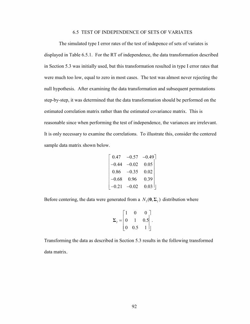
92

6.5 TEST OF INDEPENDENCE OF SETS OF VARIATES

The simulated type I error rates of the test of indepence of sets of variates is

displayed in Table 6.5.1. For the RT of independence, the data transformation described

in Section 5.3 was initially used, but this transformation resulted in type I error rates that

were much too low, equal to zero in most cases. The test was almost never rejecting the

null hypothesis. After examining the data transformation and subsequent permutations

step-by-step, it was determined that the data transformation should be performed on the

estimated correlation matrix rather than the estimated covariance matrix. This is

reasonable since when performing the test of independence, the variances are irrelevant.

It is only necessary to examine the correlations. To illustrate this, consider the centered

sample data matrix shown below.

0.47 0.57 0.490.44 0.02 0.05

0.86 0.35 0.020.68 0.96 0.390.21 0.02 0.03

− − − − − − − −

Before centering, the data were generated from a 3( , )IN 0 Σ distribution where

1 0 00 1 0.50 0.5 1

I

=

Σ .

Transforming the data as described in Section 5.3 results in the following transformed

data matrix.

93

1.26 0.81 1.510.01 0.76 0.460.52 1.50 1.42

1.77 1.18 0.650.01 0.37 0.27

− − − − − − − −

The estimated covariance matrix based on this transformed data is given by

1.00 0.78 0.00ˆ 0.78 1.00 0.25

0.00 0.25 1.00I

− = −

Σ .

In fact, the estimated covariance matrix of any set of transformed data for the test of

independence will have only ones on the diagonal. When computing the test statistic for

the observed data, the identity matrix is subtracted from ˆIΣ ; therefore, only the

correlations contribute to the magnitude of the test statistic value. Now consider a

possible permutation of this transformed data set given by

0.81 1.51 1.260.46 0.76 0.010.52 1.50 1.42

1.77 0.65 1.180.27 0.37 0.01

− − − − − − − −

.

The estimated covariance matrix of this permuted set is

0.56 0.52 0.66ˆ 0.52 1.00 0.88

0.66 0.88 0.96perm

− − = − −

Σ .

Notice now that the values on the diagonal are no longer all ones, but it is still the identity

matrix that will be subtracted from ˆpermΣ to compute the test statistic. Since the diagonal

values are not all ones, the test statistic values computed from the permuted data will

94

almost always be greater than the test statistic value resulting from the observed data.

This results in p-values very close (and often equal) to one and consequently type I error

rates very close (and often equal) to zero. Using the estimated correlation matrices rather

than the estimated covariance matrices throughout the procedure eliminates this problem

and results in much more reasonable (although still conservative) type I error rates.

These are shown in Table 6.5.1.

One additional problem arose while running the simulations for the test of

independence. When testing whether the first five variates are independent of the last

five variates with n=5 and p=10, the eigenvalues of the simulated data sets were

frequently non-positive. Recall that the data transformation described in Section 5.3

requires that, after post-multiplying the centered data by the matrix of eigenvectors, each

column be divided by the square root of the respective eigenvalue. Therefore, the

eigenvalues must be positive. Rather than entirely excluding the test of independence

between the first five and last five variates, all generated data sets that resulted in non-

positive eigenvalues were thrown out and the simulations continued until 1000 valid data

sets were randomly selected. A counter was included in the code to keep track of how

many data sets were sampled, both valid and invalid. The mean number of data sets

sampled was 3949.06 with a standard error of 27.87 (n=18). A table displaying the

number of simulated data sets for each case is shown in Appendix A.4.

The CLRT for independence appears to be the best of the CLRTs discussed in this

dissertation with respect to the simulated type I error rates. In fact, the simulated type I

error rates are within the 95% confidence bounds of 0.05 in all but eight of the 63 cases.

Also unlike the other CLRTs discussed, the CLRT for independence does not appear to

95

be affected by the underlying distribution. It performs equally well for all three

distributions. The RT appears to maintain the nominal type I error rate for p=3, but

becomes more conservative as p increases. The RT also appears to be affected by the

distribution, with the highest type I error rates usually resulting from the double

exponential data and the lowest from the uniform data. The only cases for which the RT

is more beneficial than the CLRT is when p≥n, but only for the fact that the CLRT does

not exist in these cases. Even though the RT exists in these situations it is still much too

conservative.

96

Table 6.5.1. Simulated Type I Error Rates for the Test of Independence of Sets of

Variates

a. Normal

(1, 2) (2, 3) (5, 5) (3, 3, 4) n ρ=0.2 ρ=0.5 ρ=0.8 ρ=0.2 ρ=0.5 ρ=0.8 ρ=0.2 ρ=0.5 ρ=0.8 ρ=0.2 ρ=0.5 ρ=0.8

RT 0.024 0.019 0.046* 0.023 0.028 0.039* 0.134† 0.166† 0.222† 0.020 0.021 0.045* LRT 0.333 0.310 0.299 NA NA NA NA NA NA NA NA NA 5

CLRT 0.052* 0.049* 0.052* NA NA NA NA NA NA NA NA NA RT 0.038* 0.038* 0.035 0.019 0.022 0.026 0.003 0.004 0.003 0.003 0.012 0.009

LRT 0.118 0.118 0.126 0.284 0.288 0.285 NA NA NA NA NA NA 10 CLRT 0.050* 0.043* 0.046* 0.053* 0.064 0.056* NA NA NA NA NA NA

RT 0.047* 0.063* 0.037* 0.018 0.024 0.022 0.001 0.000 0.003 0.006 0.009 0.008 LRT 0.071 0.077 0.064 0.095 0.099 0.112 0.349 0.348 0.308 0.318 0.346 0.323 25

CLRT 0.051* 0.051* 0.043* 0.049* 0.045* 0.051* 0.059* 0.056* 0.064 0.039* 0.055* 0.055*

b. Uniform

(1, 2) (2, 3) (5, 5) (3, 3, 4) n ρ=0.2 ρ=0.5 ρ=0.8 ρ=0.2 ρ=0.5 ρ=0.8 ρ=0.2 ρ=0.5 ρ=0.8 ρ=0.2 ρ=0.5 ρ=0.8

RT 0.026 0.021 0.036 0.014 0.023 0.036 0.038*† 0.072† 0.139† 0.008 0.009 0.031 LRT 0.294 0.297 0.315 NA NA NA NA NA NA NA NA NA 5

CLRT 0.041* 0.049* 0.050* NA NA NA NA NA NA NA NA NA RT 0.039* 0.032 0.028 0.007 0.011 0.012 0.000 0.000 0.002 0.001 0.001 0.004

LRT 0.124 0.123 0.124 0.284 0.289 0.285 NA NA NA NA NA NA 10 CLRT 0.054* 0.058* 0.051* 0.046* 0.060* 0.057* NA NA NA NA NA NA

RT 0.037* 0.043* 0.065 0.011 0.011 0.011 0.000 0.000 0.000 0.001 0.002 0.003 LRT 0.090 0.068 0.093 0.102 0.111 0.097 0.338 0.318 0.337 0.330 0.328 0.348 25

CLRT 0.060* 0.043* 0.065 0.055* 0.052* 0.053* 0.049* 0.052* 0.048* 0.060* 0.061* 0.067

c. Double Exponential

(1, 2) (2, 3) (5, 5) (3, 3, 4) n ρ=0.2 ρ=0.5 ρ=0.8 ρ=0.2 ρ=0.5 ρ=0.8 ρ=0.2 ρ=0.5 ρ=0.8 ρ=0.2 ρ=0.5 ρ=0.8

RT 0.037 0.031 0.056* 0.035 0.048* 0.042* 0.244† 0.257† 0.370† 0.054* 0.065 0.077 LRT 0.308 0.299 0.316 NA NA NA NA NA NA NA NA NA 5

CLRT 0.050* 0.045* 0.051* NA NA NA NA NA NA NA NA NA RT 0.043* 0.043* 0.051* 0.024 0.035 0.032 0.008 0.021 0.023 0.013 0.026 0.035

LRT 0.121 0.128 0.121 0.283 0.274 0.287 NA NA NA NA NA NA 10 CLRT 0.050* 0.066 0.052* 0.056* 0.060* 0.059* NA NA NA NA NA NA

RT 0.051* 0.040* 0.047* 0.043* 0.036 0.043* 0.004 0.007 0.006 0.017 0.013 0.015 LRT 0.085 0.081 0.074 0.118 0.109 0.116 0.349 0.346 0.357 0.343 0.326 0.341 25

CLRT 0.063* 0.057* 0.051* 0.065 0.057* 0.061* 0.055* 0.054* 0.081 0.068 0.054* 0.051* *Value is contained within 0.05 1.96 (0.05)(0.95) /1000±

†More than 1000 data sets were generated for these simulations due to non-positive eigenvalues. Data sets resulting in non-positive eigenvalues were discarded.

97

The power of the test of independence of sets of variates was investigated by

simulating multivariate data sets with covariance structure given by

11

22

kk

θ θ θ θ θ θ

ΣΣ

Σ

K

K

M M O M

K

(6.5.1)

where mmΣ , 1, ,m k= K , has the compound symmetry structure with 2 1σ = and ρ = 0.5.

The values of θ were chosen so that the covariance structure shown in (6.5.1) would be

positive definite. For example, consider the covariance structure given by

1 0.50.5 1

1 0.5 0.50.5 1 0.50.5 0.5 1

θ θ θ θ θ θ θ θ θ θ θ θ

. (6.5.2)

The determinant of (6.5.2) is 20.375 0.75− θ , which must be greater than zero if (6.5.2) is

to be positive definite. Solving this inequality yields a range of values for θ given by

( 0.7071, 0.7071)− . Therefore, θ=0.2, 0.45, and 0.7 were the values chosen to investigate

the power of the test of independence for this structure. No θ values less than 0.2 were

chosen for any of the power simulations, and the largest θ value, to the nearest tenth,

within the allowable range of θ values was chosen in each case. The simulated power of

the test of independence is displayed in Table 6.5.2.

The simulated power of the RT is very poor, never exceeding 0.444 (Uniform,

(1,2), n=25, θ=0.8), but this is somewhat expected given how conservative the test is, as

seen in Table 6.5.1. The power of the CLRT is much higher, but only exceeds 0.85 for

large θ. The CLRT still appears to be robust to non-normality; whereas the RT does not,

98

with the highest power values usually occurring for double exponential data and the

lowest for uniform data. This discrepancy is especially evident when p n≥ .

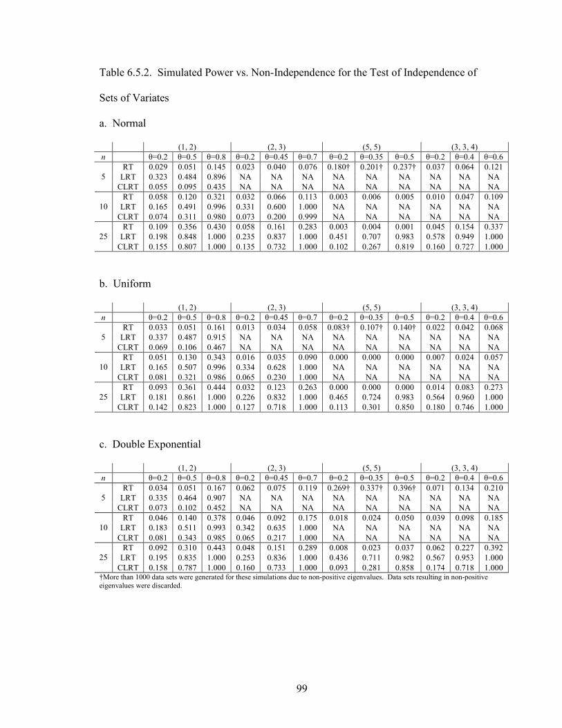
99

Table 6.5.2. Simulated Power vs. Non-Independence for the Test of Independence of

Sets of Variates

a. Normal

(1, 2) (2, 3) (5, 5) (3, 3, 4) n θ=0.2 θ=0.5 θ=0.8 θ=0.2 θ=0.45 θ=0.7 θ=0.2 θ=0.35 θ=0.5 θ=0.2 θ=0.4 θ=0.6

RT 0.029 0.051 0.145 0.023 0.040 0.076 0.180† 0.201† 0.237† 0.037 0.064 0.121 LRT 0.323 0.484 0.896 NA NA NA NA NA NA NA NA NA 5

CLRT 0.055 0.095 0.435 NA NA NA NA NA NA NA NA NA RT 0.058 0.120 0.321 0.032 0.066 0.113 0.003 0.006 0.005 0.010 0.047 0.109

LRT 0.165 0.491 0.996 0.331 0.600 1.000 NA NA NA NA NA NA 10 CLRT 0.074 0.311 0.980 0.073 0.200 0.999 NA NA NA NA NA NA

RT 0.109 0.356 0.430 0.058 0.161 0.283 0.003 0.004 0.001 0.045 0.154 0.337 LRT 0.198 0.848 1.000 0.235 0.837 1.000 0.451 0.707 0.983 0.578 0.949 1.000 25

CLRT 0.155 0.807 1.000 0.135 0.732 1.000 0.102 0.267 0.819 0.160 0.727 1.000

b. Uniform

(1, 2) (2, 3) (5, 5) (3, 3, 4) n θ=0.2 θ=0.5 θ=0.8 θ=0.2 θ=0.45 θ=0.7 θ=0.2 θ=0.35 θ=0.5 θ=0.2 θ=0.4 θ=0.6

RT 0.033 0.051 0.161 0.013 0.034 0.058 0.083† 0.107† 0.140† 0.022 0.042 0.068 LRT 0.337 0.487 0.915 NA NA NA NA NA NA NA NA NA 5

CLRT 0.069 0.106 0.467 NA NA NA NA NA NA NA NA NA RT 0.051 0.130 0.343 0.016 0.035 0.090 0.000 0.000 0.000 0.007 0.024 0.057

LRT 0.165 0.507 0.996 0.334 0.628 1.000 NA NA NA NA NA NA 10 CLRT 0.081 0.321 0.986 0.065 0.230 1.000 NA NA NA NA NA NA

RT 0.093 0.361 0.444 0.032 0.123 0.263 0.000 0.000 0.000 0.014 0.083 0.273 LRT 0.181 0.861 1.000 0.226 0.832 1.000 0.465 0.724 0.983 0.564 0.960 1.000 25

CLRT 0.142 0.823 1.000 0.127 0.718 1.000 0.113 0.301 0.850 0.180 0.746 1.000

c. Double Exponential

(1, 2) (2, 3) (5, 5) (3, 3, 4) n θ=0.2 θ=0.5 θ=0.8 θ=0.2 θ=0.45 θ=0.7 θ=0.2 θ=0.35 θ=0.5 θ=0.2 θ=0.4 θ=0.6

RT 0.034 0.051 0.167 0.062 0.075 0.119 0.269† 0.337† 0.396† 0.071 0.134 0.210 LRT 0.335 0.464 0.907 NA NA NA NA NA NA NA NA NA 5

CLRT 0.073 0.102 0.452 NA NA NA NA NA NA NA NA NA RT 0.046 0.140 0.378 0.046 0.092 0.175 0.018 0.024 0.050 0.039 0.098 0.185

LRT 0.183 0.511 0.993 0.342 0.635 1.000 NA NA NA NA NA NA 10 CLRT 0.081 0.343 0.985 0.065 0.217 1.000 NA NA NA NA NA NA

RT 0.092 0.310 0.443 0.048 0.151 0.289 0.008 0.023 0.037 0.062 0.227 0.392 LRT 0.195 0.835 1.000 0.253 0.836 1.000 0.436 0.711 0.982 0.567 0.953 1.000 25

CLRT 0.158 0.787 1.000 0.160 0.733 1.000 0.093 0.281 0.858 0.174 0.718 1.000 †More than 1000 data sets were generated for these simulations due to non-positive eigenvalues. Data sets resulting in non-positive eigenvalues were discarded.

100

CHAPTER 7

CONCLUSIONS

For all of the covariance structures discussed in Chapter 6, the RT has one

definite advantage over the CLRT; the RT exists when p n≥ in which case the CLRT

does not. And although the simulated type I error rates of the RT were usually much too

high in these cases, it is still an advantage that the RT exists at all when p n≥ . Due to

the existence of the RT in these cases, perhaps a corrected RT, similar to the CLRT, can

be derived to improve the simulated type I error rates.

For all of the tests except the test of independence of sets of variates, the RT has

another advantage over the CLRT in that the data distribution does not have as extreme

an effect on the simulated type I error rates and power of the RT as it does on the CLRT.

As discussed in Chapter 6, there does appear to be some distributional effect on the RT;

however, the effect is very small in most cases and much less than for the CLRT in all

cases. The CLRT for independence performs very well with respect to the simulated type

I error rates for any underlying distribution, even for very small sample sizes; therefore,

there does not appear to be any distributional advantage of the RT over the CLRT for

testing for this structure.

The RTs for sphericity, compound symmetry, and type H all appear to be α-level

tests, but they tend to have very low power versus certain alternative structures. The RT

for sphericity has poor power versus non-zero correlation and serial correlation; the RT

101

for compound symmetry has poor power versus serial correlation; and the RT for type H

has poor power versus serial correlation when p is small. Notice that in each of these

cases the null covariance structures differ from the alternative covariance structures by

only correlations. Consequently, the test statistic used in the RT appears to be good at

detecting differences in the variances, but has a difficult time detecting differences in

only the correlations.

The RT does not appear to be an α-level test when testing for serial correlation or

independence of sets of variates. From the results shown in Appendix A.3, it appears that

the simulated type I error rates of the RT of serial correlation can be improved by

eliminating the bias in the MLEs of ρ and 2σ , but this hypothesis needs to be investigated

further. The RT of independence, on the other hand, really does not warrant further

investigation due to the strong performance of the CLRT of independence.

Although improvements to the RT need to be made when testing for several of the

covariance structures discussed in this dissertation, the simulations have shown some

promise. Overall, the RT appears to be a legitimate alternative to the CLRT when p n≥ ,

or the data are not normally distributed when testing for spericity, compound symmetry,

type H, or serial correlation. Recall also, from Chapter 4, that RTs do not require random

sampling. Random assignment of experimental units to treatments will suffice.

Therefore, there are several situations for which an RT for the structure of a covariance

matrix can be beneficial.

102

CHAPTER 8

FUTURE WORK

There are several additional problems related to this material that I would like to

explore. The most obvious of these is to apply this test to covariance structures that I

have not already studied, specifically factor analysis and structural equation modeling

among others. I have already completed the literature review for these procedures, but I

foresee several difficulties in writing the code to perform these tests. First, there isn’t a

specific structure in factor analysis/structural equation modeling. The structure is driven

by the data and the researcher’s intuition about the number of underlying factors.

Therefore, the code will need to be altered for each structure. Second, the MLEs must be

found numerically which could add a considerable amount of computing time. Finally,

there is the issue of determining exactly what models to test since there is no specific

structure. Other structures, such as those used in time series, should not require much

additional work other than researching the likelihood ratio tests for these structures,

changing the R code slightly, and running additional simulations.

I am also interested in determining the effect of changing the test statistic used for

the RT. Currently, the RT is based on the absolute differences between the variances and

covariances. I would like to do a Monte Carlo study using a test statistic based on the

squared differences between the variances and covariances. I anticipate that this will

103

have no significant effect on the simulated type I error rates and power of the RT, but it is

worth exploring. I have also noticed that the RT is better at detecting differences in the

variances than differences in the correlations. After thinking about the formula for

covariance, which is a function of the variances and correlation, I realized that in using

the test statistic based on the differences in the variances and covariances, I was

essentially ‘counting’ the differences in the variances twice. Therefore, I think the test

statistic could be improved by using the difference in the variances and correlations

rather than the differences in the variances and covariances.

There are also several closely related problems that arose during the development

of the permutation test for the structure of a covariance matrix. In writing the code for

the simulations, I had some difficulty finding adequate algorithms for generating

multivariate random samples with specified covariance structures from non-normal

distributions. As a result, I ended up using two different procedures, one for each of the

non-normal distributions studied. Neither of these procedures was user friendly or

accurate with respect to the desired covariance structure, especially in small samples.

The current procedures are based on transforming independent normally distributed

univariate data sets to achieve a multivariate non-normal data set with a desired

covariance structure. Virtually all statistical software packages have built-in functions

for generating data from many univariate non-normal distributions. I think a new

procedure may be possible by applying a data transformation to univariate non-normal

data generated using the built-in functions.

I have also noticed some unusual results for the RT of serial correlation. I think

these unusual results are related to the biased nature of the MLEs that were used (See

104

Appendix A.3). Consequently, I would like to see what would happen to the simulated

type I error rates and power if unbiased estimates are used instead. For the serial

correlation, there are two parameters that must be estimated, ρ and 2σ , and the MLE of

2σ is actually a function of the MLE of ρ . Through simulation I have determined that

there is a simple multiplicative correction factor for the MLE of 2σ if the estimate of ρ

is unbiased (See Appendix A.3); however, there does not exist a closed form of the bias

of the MLE of ρ and based on simulations there appears to be a quadratic relationship

between the bias of the MLE of ρ and the true value of ρ . I am interested in

determining a bias correction factor for the MLE of ρ and using these unbiased estimates

to see if the simulated type I error rates and power of the permutation test of serial

correlation would improve.

105

BIBLIOGRAPHY

Anderson, T.W. (2003). An Introduction to Multivariate Statistical Analysis (3rd ed.).

Hoboken, NJ: John Wiley & Sons.

Boik, R.J. (1975). Interactions in the analysis of variance: A procedure for interpretation

and a Monte Carlo comparison of univariate and multivariate methods for

repeated measures designs. Dissertation Abstracts International, 36(06), 2908B.

(UMI No. 7527837).

Boik, R.J. (1981). A priori tests in repeated measures designs: Effects of nonsphericity.

Psychometrika, 46(3), 241-255.

Bollen, K.A. & Stine, R.A. (1993). Bootstrapping goodness-of-fit measures in structural

equation models. In K.A. Bollen & J.S. Long (Eds.), Testing Structural Equation

Models (pp. 111-135). Newbury Park, CA: Sage Publications.

Box, G.E.P. (1949). A general distribution theory for a class of likelihood criteria.

Biometrika, 36, 317-346

Box, G.E.P. (1950). Problems in the analysis of growth and wear curves. Biometrics,

6(4), 362-389.

Box, G.E.P. (1954). Some theorems on quadratic forms applied in the study of analysis of

variance problems, II. Effects of inequality of variance and of correlation between

errors in the two-way classification. The Annals of Mathematical Statistics, 25(3),

484-498.

106

Carter, E.M. & Srivastava, M.S. (1983). Asymptotic non-null distribution for the locally

most powerful invariant test for sphericity. Communications in Statistics: Theory

and Methods, 12(15), 1719-1725.

Cheang, W-K. & Reinsel, G.C. (2000). Bias reduction of autoregressive estimates in time

series regression model through restricted maximum likelihood. Journal of the

American Statistical Association, 95(452), 1173-1184.

Consul, P.C. (1967a). On the exact distributions of the criterion W for testing sphericity

in a p-variate normal distribution. The Annals of Mathematical Statistics, 38(4),

1170-1174.

Consul, P.C. (1967b). On the exact distributions of likelihood ratio criteria for testing

independence of sets of variates under the null hypothesis. The Annals of

Mathematical Statistics, 38(4), 1160-1169.

Cornell, J.E., Young, D.M., Seaman, S.L., & Kirk R.E. (1992). Power comparisons of

eight tests for sphericity in repeated measures designs. Journal of Educational

Statistics, 17(3), 233-249.

Dwass, M. (1957). Modified randomization tests for nonparametric hypotheses. The

Annals of Mathematical Statistics, 28, 181-187.

Edgington, E.S. (1995). Randomization Tests (3rd ed.). New York: Marcel Dekker.

Falk, M. (1999). A simple approach to the generation of uniformly distributed random

variables with prescribed correlations. Communications in Statistics: Simulation

and Computation, 28(3), 785-791.

Fisher, R.A. (1936). The coefficient of racial likeness and the future of craniometry. The

Journal of the Anthropological Institute of Great Britain and Ireland, 66, 57-63.

107

Fisher, R.A. (1971). The Design of Experiments (9th ed.). New York: Hafner Press.

Geisser, S. & Greenhouse, S.W. (1958). An extension of Box’s results on the use of the F

distribution in multivariate analysis. The Annals of Mathematical Statistics, 29(3),

885-891.

Gerbing, D.W. & Anderson, J.C. (1993). Monte Carlo evaluations of goodness-of-fit

indices for structural equation models. In K.A. Bollen & J.S. Long (Eds.), Testing

Structural Equation Models (pp. 40-65). Newbury Park, CA: Sage Publications.

Good, P. (1994). Permutation Tests: A Practical Guide to Resampling Methods for

Testing Hypotheses. New York: Springer-Verlag.

Good, P. (2002). Extensions of the concept of exchangeability and their applications.

Journal of Modern Applied Statistical Methods, 1(2), 243-247.

Graybill, F.A. (1983). Matrices with Applications in Statistics (2nd ed.). Belmont, CA:

Duxbury.

Headrick, T.C. (2002). Fast fifth-order polynomial transforms for generating univariate

and multivariate nonnormal distributions. Computational Statistics & Data

Analysis, 40, 685-711.

Hearne, E.M. & Clark, G.M. (1983). Validity and power investigation of a test for serial

correlation in univariate repeated measures analysis. Statistics in Medicine, 2,

497-504.

Hearne, E.M., Clark, G.M., & Hatch, J.P. (1983). A test for serial correlation in

univariate repeated-measures analysis. Biometrics, 39(1), 237-243.

108

Huynh, H. & Feldt, L.S. (1970). Conditions under which mean square ratios in repeated

measurements designs have exact F-distributions. Journal of the American

Statistical Association, 65, 1582-1589.

Huynh, H. & Mandeville, G.K. (1979). Validity conditions in repeated measures designs.

Psychological Bulletin, 86(5), 964-973.

John, S. (1971). Some optimal multivariate tests. Biometrika, 58(1), 123-127.

John, S. (1972). The distribution of a statistic used for testing sphericity of normal

distributions. Biometrika, 59(1), 169-173.

Keselman, H.J., Rogan, J.C., Mendoza, J.L., & Breen, L.J. (1980). Testing the validity

conditions of repeated measures F tests. Psychological Bulletin, 87(3), 479-481.

Khatri, C.G. (1978). Some optimization problems with applications to canonical

correlations and sphericity tests. Journal of multivariate analysis, 8, 453-467.

Krishnaiah, P.R. & Waikar, V.B. (1972). Simultaneous tests for equality of latent roots

against certain alternatives – II. Annals of the Institute of Statistical Mathematics,

24(1), 81-85.

Krzanowski, W.J. (1993). Permutational tests for correlation matrices. Statistics and

Computing, 3, 37-44.

Kuehl, R.O. (2000). Design of Experiments: Statistical Principles of Research Design

and Analysis (2nd ed.). Pacific Grove, CA: Duxbury.

Lawley, D.N. & Maxwell, A.E. (1971). Factor Analysis as a Statistical Method (2nd ed.).

London: Butterworths.

109

Magee, L. (1989). Bias approximations for covariance parameter estimators in the linear

model with AR(1) errors. Communications in Statistics: Theory and Methods,

18(2), 395-422.

Manly, B.F.J. (1997). Randomization and Monte Carlo Methods in Biology (2nd ed.).

London: Chapman & Hall.

Mauchly, J.W. (1940). Significance test for sphericity of a normal n-variate distribution.

The Annals of Mathematical Statistics, 11(2), 204-209.

Nagarsenker, B.N. & Pillai, K.C.S. (1973a). Distribution of the likelihood ratio criterion

for testing a hypothesis specifying a covariance matrix. Biometrika, 60(2), 359-

364.

Nagarsenker, B.N. & Pillai, K.C.S. (1973b). The distribution of the sphericity test

criterion. Journal of Multivariate Analysis, 3, 226-235.

Pitman, E.J.G. (1937a). Significance tests which may be applied to samples from any

populations. Journal of the Royal Statistical Society, Series B, 4, 119-130.

Pitman, E.J.G. (1937b). Significance tests which may be applied to samples from any

populations. II. The correlation coefficient. Journal of the Royal Statistical

Society, Series B, 4, 225-232.

Pitman, E.J.G. (1938). Significance tests which may be applied to samples from any

populations. III. The analysis of variance test. Biometrika, 29, 322-335.

Rouanet, H. & Lepine, D. (1970). Comparison between treatments in a repeated-

measurement design: ANOVA and multivariate methods. The British Journal of

Mathematical and Statistical Psychology, 23(2), 147-163.

110

Shipley, B. (2000). A permutation procedure for testing the equality of pattern

hypotheses across groups involving correlation or covariance matrices. Statistics

and Computing, 10, 253-257.

Srivastava, M.S. & Khatri, C.G. (1979). An Introduction to Multivariate Statistics. New

York: North Holland.

Sugiura, N. (1972). Locally best invariant test for sphericity and the limiting

distributions. The Annals of Mathematical Statistics, 43(4), 1312-1316.

Vale, C.D. & Maurelli, V.A. (1983). Simulating multivariate nonnormal distributions.

Psychometrika, 48(3), 465-471.

Venables, W. (1976). Some implications of the union-intersection principle for tests of

sphericity. Journal of Multivariate Analysis, 6, 185-190.

Wald, A. & Brookner, R.J. (1941). On the distribution of Wilks’ statistic for testing the

independence of several groups of variates. The Annals of Mathematical

Statistics, 12(2), 137-152.

Wilks, S.S. (1935). On the independence of k sets of normally distributed statistical

variables. Econometrica, 3(3), 309-326.

Wilks, S.S. (1946). Sample criteria for testing equality of means, equality of variances,

and equality of covariances in a normal multivariate distribution. The Annals of

Mathematical Statistics, 17(3), 257-281.

Zhu, L-X, Ng, K.W., & Jing, P. (2003). Resampling methods for homogeneity tests of

covariance matrices. Statistica Sinica, 12, 769-783.

111

APPENDIX

A.1 R CODE

The following code was written for R version 2.3.1 and was used to run the

simulations described in Chapter 6.

A.1.1 RANDOMIZATION TEST OF SPHERICITY

## Test of Sphericity ## library(MASS) #Function to perform the test of sphericity with multivariate normal #data. Inputs are n=sample size; cov.mat=simulated covariance matrix; #struc="S", "NH", "CS", "TH", or "SC"; par1 & par2=the two parameter #values used to generate the covariance matrix; K=number of simulations spher.norm<-function(n, cov.mat, struc, par1, par2, K) { dist<-"norm" p<-dim(cov.mat)[1] df<-.5*p*(p+1)-1 crit<-qchisq(.95, df) C<-1-(2*p^2+p+2)/(6*p*(n-1)) perm<-matrix(NA, n, p) count.rt<-0 count.lr<-0 count.lrc<-0 if (n>p) { for (i in 1:K) { dat<-mvrnorm(n, vector("integer", p), cov.mat) cov.dat<-(n-1)/n*var(dat) est.var<-mean(diag(cov.dat)) #Likelihood Ratio Test L.S<-det(cov.dat)/(1/p*sum(diag(cov.dat)))^p if (-n*log(L.S) > crit) count.lr<-count.lr+1 #Corrected Likelihood Ratio Test if (-C*(n-1)*log(L.S) > crit) count.lrc<-count.lrc+1 #Randomization Test est.cov.mat<-est.var*diag(p) ts.dat<-0 for (j in 1:p) { ts.dat<-ts.dat+sum(abs(cov.dat[j,j:p]-est.cov.mat[j,j:p])) }

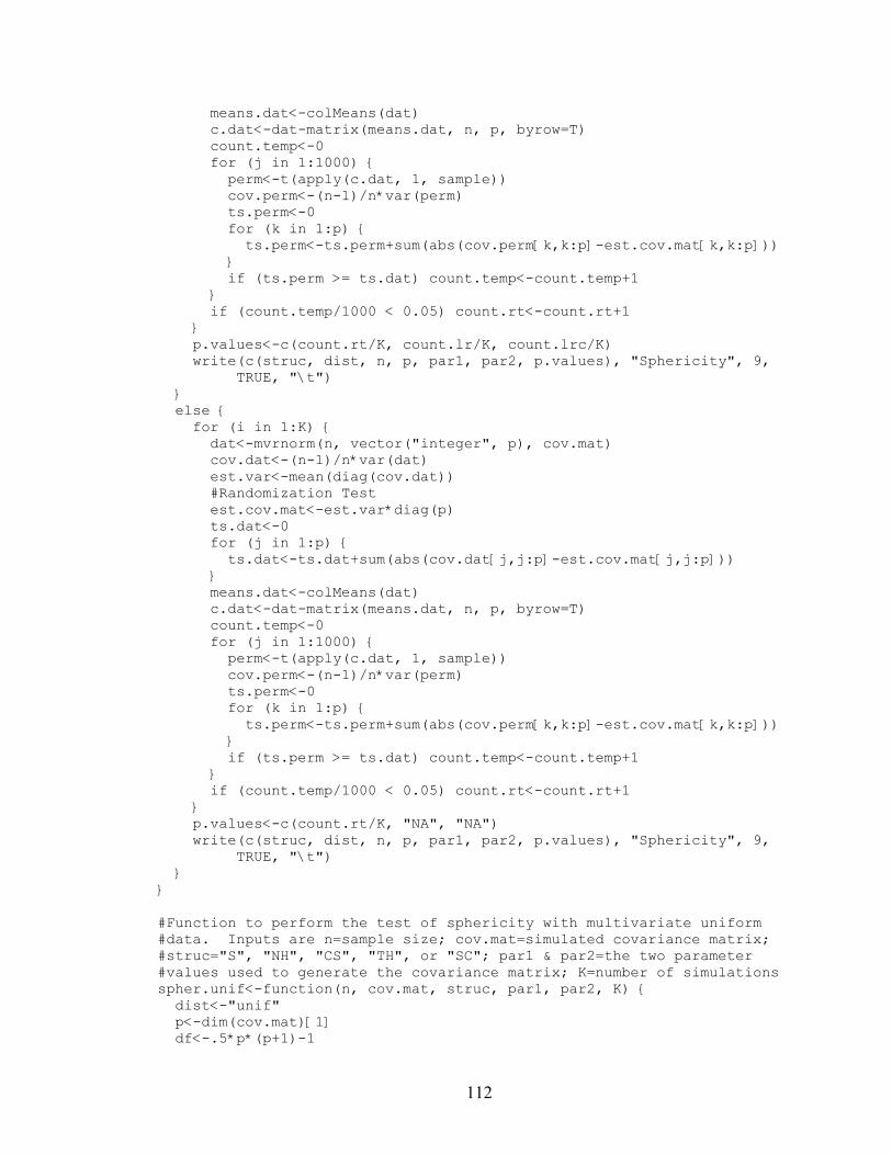
112

means.dat<-colMeans(dat) c.dat<-dat-matrix(means.dat, n, p, byrow=T) count.temp<-0 for (j in 1:1000) { perm<-t(apply(c.dat, 1, sample)) cov.perm<-(n-1)/n*var(perm) ts.perm<-0 for (k in 1:p) { ts.perm<-ts.perm+sum(abs(cov.perm[k,k:p]-est.cov.mat[k,k:p])) }

if (ts.perm >= ts.dat) count.temp<-count.temp+1 } if (count.temp/1000 < 0.05) count.rt<-count.rt+1 }

p.values<-c(count.rt/K, count.lr/K, count.lrc/K) write(c(struc, dist, n, p, par1, par2, p.values), "Sphericity", 9, TRUE, "\t") }

else { for (i in 1:K) { dat<-mvrnorm(n, vector("integer", p), cov.mat) cov.dat<-(n-1)/n*var(dat) est.var<-mean(diag(cov.dat)) #Randomization Test est.cov.mat<-est.var*diag(p) ts.dat<-0 for (j in 1:p) { ts.dat<-ts.dat+sum(abs(cov.dat[j,j:p]-est.cov.mat[j,j:p])) } means.dat<-colMeans(dat) c.dat<-dat-matrix(means.dat, n, p, byrow=T) count.temp<-0 for (j in 1:1000) { perm<-t(apply(c.dat, 1, sample)) cov.perm<-(n-1)/n*var(perm) ts.perm<-0 for (k in 1:p) { ts.perm<-ts.perm+sum(abs(cov.perm[k,k:p]-est.cov.mat[k,k:p])) }

if (ts.perm >= ts.dat) count.temp<-count.temp+1 } if (count.temp/1000 < 0.05) count.rt<-count.rt+1 }

p.values<-c(count.rt/K, "NA", "NA") write(c(struc, dist, n, p, par1, par2, p.values), "Sphericity", 9, TRUE, "\t") }}

#Function to perform the test of sphericity with multivariate uniform #data. Inputs are n=sample size; cov.mat=simulated covariance matrix; #struc="S", "NH", "CS", "TH", or "SC"; par1 & par2=the two parameter #values used to generate the covariance matrix; K=number of simulations spher.unif<-function(n, cov.mat, struc, par1, par2, K) { dist<-"unif" p<-dim(cov.mat)[1] df<-.5*p*(p+1)-1

113

crit<-qchisq(.95, df) C<-1-(2*p^2+p+2)/(6*p*(n-1)) perm<-matrix(NA, n, p) count.rt<-0 count.lr<-0 count.lrc<-0 corr.mat<-cov.mat for (i in 1:p) { for (j in i:p) { corr.mat[i,j]<-2*sin((pi/6)*(cov.mat[i,j]/sqrt(cov.mat[i,i]*

cov.mat[j,j]))) corr.mat[j,i]<-corr.mat[i,j] }

}if (n>p) {

for (i in 1:K) { unif01.dat<-pnorm(mvrnorm(n, vector("integer", p), corr.mat)) dat<-t(sqrt(12*diag(cov.mat))*t(unif01.dat)) cov.dat<-(n-1)/n*var(dat) est.var<-mean(diag(cov.dat)) #Likelihood Ratio Test L.S<-det(cov.dat)/(1/p*sum(diag(cov.dat)))^p if (-n*log(L.S) > crit) count.lr<-count.lr+1 #Corrected Likelihood Ratio Test if (-C*(n-1)*log(L.S) > crit) count.lrc<-count.lrc+1 #Randomization Test est.cov.mat<-est.var*diag(p) ts.dat<-0 for (j in 1:p) { ts.dat<-ts.dat+sum(abs(cov.dat[j,j:p]-est.cov.mat[j,j:p])) } means.dat<-colMeans(dat) c.dat<-dat-matrix(means.dat, n, p, byrow=T) count.temp<-0 for (j in 1:1000) { perm<-t(apply(c.dat, 1, sample)) cov.perm<-(n-1)/n*var(perm) ts.perm<-0 for (k in 1:p) { ts.perm<-ts.perm+sum(abs(cov.perm[k,k:p]-est.cov.mat[k,k:p])) }

if (ts.perm >= ts.dat) count.temp<-count.temp+1 } if (count.temp/1000 < 0.05) count.rt<-count.rt+1 }

p.values<-c(count.rt/K, count.lr/K, count.lrc/K) write(c(struc, dist, n, p, par1, par2, p.values), "Sphericity", 9, TRUE, "\t") }

else { for (i in 1:K) { unif01.dat<-pnorm(mvrnorm(n, vector("integer", p), corr.mat)) dat<-t(sqrt(12*diag(cov.mat))*t(unif01.dat)) cov.dat<-(n-1)/n*var(dat) est.var<-mean(diag(cov.dat)) #Randomization Test est.cov.mat<-est.var*diag(p)

114

ts.dat<-0 for (j in 1:p) { ts.dat<-ts.dat+sum(abs(cov.dat[j,j:p]-est.cov.mat[j,j:p])) } means.dat<-colMeans(dat) c.dat<-dat-matrix(means.dat, n, p, byrow=T) count.temp<-0 for (j in 1:1000) { perm<-t(apply(c.dat, 1, sample)) cov.perm<-(n-1)/n*var(perm) ts.perm<-0 for (k in 1:p) { ts.perm<-ts.perm+sum(abs(cov.perm[k,k:p]-est.cov.mat[k,k:p])) }

if (ts.perm >= ts.dat) count.temp<-count.temp+1 } if (count.temp/1000 < 0.05) count.rt<-count.rt+1 }

p.values<-c(count.rt/K, "NA", "NA") write(c(struc, dist, n, p, par1, par2, p.values), "Sphericity", 9, TRUE, "\t") }}

#Function to perform the test of sphericity with multivariate double #exponential data. Inputs are n=sample size; cov.mat=simulated #covariance matrix; struc="S", "NH", "CS", "TH", or "SC"; par1 & #par2=the two parameter values used to generate the covariance matrix; #K=number of simulations spher.de<-function(n, cov.mat, struc, par1, par2, K) { dist<-"de" p<-dim(cov.mat)[1] b<-0.7824 d<-0.0679 c1<-b^2+6*b*d+9*d^2 c2<-6*d^2 df<-.5*p*(p+1)-1 crit<-qchisq(.95, df) C<-1-(2*p^2+p+2)/(6*p*(n-1)) perm<-matrix(NA, n, p) count.rt<-0 count.lr<-0 count.lrc<-0 corr.mat<-cov.mat for (i in 1:p) { for (j in i:p) { corr.mat[i,j]<-cov.mat[i,j]/sqrt(cov.mat[i,i]*cov.mat[j,j]) corr.mat[j,i]<-corr.mat[i,j] }

}corr.int<-corr.mat

for (j in 1:(p-1)) { for (k in (j+1):p) { corr.int[j,k]<-Re(polyroot(c(-corr.mat[j,k],c1,0,c2))[1]) corr.int[k,j]<-corr.int[j,k] }

}

115

if (n>p) { for (i in 1:K) { norm.dat<-mvrnorm(n, vector("integer", p), corr.int) dat<-t(sqrt(diag(cov.mat))*t(b*norm.dat+d*norm.dat^3)) cov.dat<-(n-1)/n*var(dat) est.var<-mean(diag(cov.dat)) #Likelihood Ratio Test L.S<-det(cov.dat)/(1/p*sum(diag(cov.dat)))^p if (-n*log(L.S) > crit) count.lr<-count.lr+1 #Corrected Likelihood Ratio Test if (-C*(n-1)*log(L.S) > crit) count.lrc<-count.lrc+1 #Randomization Test est.cov.mat<-est.var*diag(p) ts.dat<-0 for (j in 1:p) { ts.dat<-ts.dat+sum(abs(cov.dat[j,j:p]-est.cov.mat[j,j:p])) } means.dat<-colMeans(dat) c.dat<-dat-matrix(means.dat, n, p, byrow=T) count.temp<-0 for (j in 1:1000) { perm<-t(apply(c.dat, 1, sample)) cov.perm<-(n-1)/n*var(perm) ts.perm<-0 for (k in 1:p) { ts.perm<-ts.perm+sum(abs(cov.perm[k,k:p]-est.cov.mat[k,k:p])) }

if (ts.perm >= ts.dat) count.temp<-count.temp+1 } if (count.temp/1000 < 0.05) count.rt<-count.rt+1 }

p.values<-c(count.rt/K, count.lr/K, count.lrc/K) write(c(struc, dist, n, p, par1, par2, p.values), "Sphericity", 9, TRUE, "\t") }

else { for (i in 1:K) { norm.dat<-mvrnorm(n, vector("integer", p), corr.int) dat<-t(sqrt(diag(cov.mat))*t(b*norm.dat+d*norm.dat^3)) cov.dat<-(n-1)/n*var(dat) est.var<-mean(diag(cov.dat)) #Randomization Test est.cov.mat<-est.var*diag(p) ts.dat<-0 for (j in 1:p) { ts.dat<-ts.dat+sum(abs(cov.dat[j,j:p]-est.cov.mat[j,j:p])) } means.dat<-colMeans(dat) c.dat<-dat-matrix(means.dat, n, p, byrow=T) count.temp<-0 for (j in 1:1000) { perm<-t(apply(c.dat, 1, sample)) cov.perm<-(n-1)/n*var(perm) ts.perm<-0 for (k in 1:p) { ts.perm<-ts.perm+sum(abs(cov.perm[k,k:p]-est.cov.mat[k,k:p])) }

116

if (ts.perm >= ts.dat) count.temp<-count.temp+1 } if (count.temp/1000 < 0.05) count.rt<-count.rt+1 }

p.values<-c(count.rt/K, "NA", "NA") write(c(struc, dist, n, p, par1, par2, p.values), "Sphericity", 9, TRUE, "\t") }}K<-1000 #Type I Error for (n in c(5, 10, 25)) { for (p in c(3, 5, 10)) { for (var in c(1, 9, 25)) { cov.mat<-var*diag(p) spher.norm(n, cov.mat, "S", var, 0, K) spher.unif(n, cov.mat, "S", var, 0, K) spher.de(n, cov.mat, "S", var, 0, K) }

}}#Power vs. Non-Homoscedasticity for (n in c(5, 10, 25)) { for (p in c(3, 5, 10)) { for (var.diff in c(4, 8, 12)) { cov.mat<-diag(c(matrix(seq(1, 1+var.diff, by=var.diff/(p-1)), 1,

p))) spher.norm(n, cov.mat, "NH", var.diff, 0, K) spher.unif(n, cov.mat, "NH", var.diff, 0, K) spher.de(n, cov.mat, "NH", var.diff, 0, K) }

}}#Power vs. Non-Zero Correlation var<-1 for (n in c(5, 10, 25)) { for (p in c(3, 5, 10)) { for (rho in c(0.3, 0.6, 0.9)) { cov.mat<-var*((1-rho)*diag(p)+matrix(rho,p,p)) spher.norm(n, cov.mat, "CS", var, rho, K) spher.unif(n, cov.mat, "CS", var, rho, K) spher.de(n, cov.mat, "CS", var, rho, K) }

}}#Power vs. Type H p<-3 for (n in c(5, 10, 25)) { for (lambda in c(2, 3, 4)) { for (diff in c(lambda-1, lambda, lambda+1)) { cov.mat<-diag(seq(1, (p-1)*diff+1, by=diff)) for (i in 1:(p-1)) { for (j in (i+1):p) { cov.mat[i,j]<-0.5*(cov.mat[i,i]+cov.mat[j,j])-lambda cov.mat[j,i]<-cov.mat[i,j] }

}

117

spher.norm(n, cov.mat, "TH", lambda, diff, K) spher.unif(n, cov.mat, "TH", lambda, diff, K) spher.de(n, cov.mat, "TH", lambda, diff, K) }

}}p<-5 for (n in c(5, 10, 25)) { for (lambda in c(1.25, 1.5)) { for (diff in c(2*lambda/5-.4, 2*lambda/5, 2*lambda/5+.4)) { cov.mat<-diag(seq(1, (p-1)*diff+1, by=diff)) for (i in 1:(p-1)) { for (j in (i+1):p) { cov.mat[i,j]<-0.5*(cov.mat[i,i]+cov.mat[j,j])-lambda cov.mat[j,i]<-cov.mat[i,j] }

}spher.norm(n, cov.mat, "TH", lambda, diff, K)

spher.unif(n, cov.mat, "TH", lambda, diff, K) spher.de(n, cov.mat, "TH", lambda, diff, K) }

}}lambda<-1 for (n in c(5, 10, 25)) { for (diff in c(0.1, 0.4, 0.8)) { cov.mat<-diag(seq(1, (p-1)*diff+1, by=diff)) for (i in 1:(p-1)) { for (j in (i+1):p) { cov.mat[i,j]<-0.5*(cov.mat[i,i]+cov.mat[j,j])-lambda cov.mat[j,i]<-cov.mat[i,j] } }

spher.norm(n, cov.mat, "TH", lambda, diff, K) spher.unif(n, cov.mat, "TH", lambda, diff, K) spher.de(n, cov.mat, "TH", lambda, diff, K) }}p<-10 for (n in c(5, 10, 25)) { for (lambda in c(0.5, 0.75, 1)) { for (diff in c(.1, .1+(2*lambda+1)/50, .1+(2*lambda+1)/25)) { cov.mat<-diag(seq(1, (p-1)*diff+1, by=diff)) for (i in 1:(p-1)) { for (j in (i+1):p) { cov.mat[i,j]<-0.5*(cov.mat[i,i]+cov.mat[j,j])-lambda cov.mat[j,i]<-cov.mat[i,j] }

}spher.norm(n, cov.mat, "TH", lambda, diff, K)

spher.unif(n, cov.mat, "TH", lambda, diff, K) spher.de(n, cov.mat, "TH", lambda, diff, K) }

}}#Power vs. Serial Correlation sigma<-1

118

for (n in c(5, 10, 25)) { for (p in c(3, 5, 10)) { for (rho in c(0.3, 0.6, 0.9)) { cov.mat<-(sigma^2/(1-rho^2))*diag(p) for (i in 1:(p-1)) { for (j in (i+1):p) { cov.mat[i,j]<-(sigma^2/(1-rho^2))*rho^(j-i) cov.mat[j,i]<-cov.mat[i,j] }

}spher.norm(n, cov.mat, "SC", sigma, rho, K)

spher.unif(n, cov.mat, "SC", sigma, rho, K) spher.de(n, cov.mat, "SC", sigma, rho, K) }

}}

A.1.2 RANDOMIZATION TEST OF COMPOUND SYMMETRY

## Test of Compound Symmetry ## library(MASS) #Function to perform the test of compound symmetry with multivariate #normal data. Inputs are n=sample size; cov.mat=simulated covariance #matrix; struc="CS", "TH", or "SC"; par1 & par2=the two parameter #values used to generate the covariance matrix; K=number of simulations compsym.norm<-function(n, cov.mat, struc, par1, par2, K) { dist<-"norm" p<-dim(cov.mat)[1] df<-.5*p*(p+1)-2 crit<-qchisq(.95, df) C<-1-(p*(p+1)^2*(2*p-3))/(6*(n-1)*(p-1)*(p^2+p-4)) perm<-matrix(NA, n, p) count.rt<-0 count.lr<-0 count.lrc<-0 if (n>p) { for (i in 1:K) { dat<-mvrnorm(n, vector("integer", p), cov.mat) cov.dat<-(n-1)/n*var(dat) est.var<-mean(diag(cov.dat)) est.corr<-mean(cov.dat[cov.dat!=diag(cov.dat)])/est.var #Likelihood Ratio Test L.CS<-det(cov.dat)/(est.var^p*(1-est.corr)^(p-1)*(1+(p-1)*

est.corr)) if (-n*log(L.CS) > crit) count.lr<-count.lr+1 #Corrected Likelihood Ratio Test if (-C*(n-1)*log(L.CS) > crit) count.lrc<-count.lrc+1 #Randomization Test est.cov.mat<-est.var*((1-est.corr)*diag(p)+matrix(est.corr, p,

p)) ts.dat<-0 for (j in 1:p) { ts.dat<-ts.dat+sum(abs(cov.dat[j,j:p]-est.cov.mat[j,j:p]))

119

}means.dat<-colMeans(dat)

c.dat<-dat-matrix(means.dat, n, p, byrow=T) count.temp<-0 for (j in 1:1000) { perm<-t(apply(c.dat, 1, sample)) cov.perm<-(n-1)/n*var(perm) ts.perm<-0 for (k in 1:p) { ts.perm<-ts.perm+sum(abs(cov.perm[k,k:p]-est.cov.mat[k,k:p])) }

if (ts.perm >= ts.dat) count.temp<-count.temp+1 } if (count.temp/1000 < 0.05) count.rt<-count.rt+1 }

p.values<-c(count.rt/K, count.lr/K, count.lrc/K) write(c(struc, dist, n, p, par1, par2, p.values), "Compound Symmetry", 9, TRUE, "\t") }

else { for (i in 1:K) { dat<-mvrnorm(n, vector("integer", p), cov.mat) cov.dat<-(n-1)/n*var(dat) est.var<-mean(diag(cov.dat)) est.corr<-mean(cov.dat[cov.dat!=diag(cov.dat)])/est.var #Randomization Test est.cov.mat<-est.var*((1-est.corr)*diag(p)+matrix(est.corr, p,

p)) ts.dat<-0 for (j in 1:p) { ts.dat<-ts.dat+sum(abs(cov.dat[j,j:p]-est.cov.mat[j,j:p])) } means.dat<-colMeans(dat) c.dat<-dat-matrix(means.dat, n, p, byrow=T) count.temp<-0 for (j in 1:1000) { perm<-t(apply(c.dat, 1, sample)) cov.perm<-(n-1)/n*var(perm) ts.perm<-0 for (k in 1:p) { ts.perm<-ts.perm+sum(abs(cov.perm[k,k:p]-est.cov.mat[k,k:p])) }

if (ts.perm >= ts.dat) count.temp<-count.temp+1 } if (count.temp/1000 < 0.05) count.rt<-count.rt+1 }

p.values<-c(count.rt/K, NA, NA) write(c(struc, dist, n, p, par1, par2, p.values), "Compound Symmetry", 9, TRUE, "\t") }}

#Function to perform the test of compound symmetry with multivariate #uniform data. Inputs are n=sample size; cov.mat=simulated covariance #matrix; struc="CS", "TH", or "SC"; par1 & par2=the two parameter #values used to generate the covariance matrix; K=number of simulations compsym.unif<-function(n, cov.mat, struc, par1, par2, K) {

120

dist<-"unif" p<-dim(cov.mat)[1] df<-.5*p*(p+1)-2 crit<-qchisq(.95, df) C<-1-(p*(p+1)^2*(2*p-3))/(6*(n-1)*(p-1)*(p^2+p-4)) perm<-matrix(NA, n, p) count.rt<-0 count.lr<-0 count.lrc<-0 corr.mat<-cov.mat for (i in 1:p) { for (j in i:p) { corr.mat[i,j]<-2*sin((pi/6)*(cov.mat[i,j]/sqrt(cov.mat[i,i]*

cov.mat[j,j]))) corr.mat[j,i]<-corr.mat[i,j] }

}if (n>p) {

for (i in 1:K) { unif01.dat<-pnorm(mvrnorm(n, vector("integer", p), corr.mat)) dat<-t(sqrt(12*diag(cov.mat))*t(unif01.dat)) cov.dat<-(n-1)/n*var(dat) est.var<-mean(diag(cov.dat)) est.corr<-mean(cov.dat[cov.dat!=diag(cov.dat)])/est.var #Likelihood Ratio Test L.CS<-det(cov.dat)/(est.var^p*(1-est.corr)^(p-1)*(1+(p-1)*

est.corr)) if (-n*log(L.CS) > crit) count.lr<-count.lr+1 #Corrected Likelihood Ratio Test if (-C*(n-1)*log(L.CS) > crit) count.lrc<-count.lrc+1 #Randomization Test est.cov.mat<-est.var*((1-est.corr)*diag(p)+matrix(est.corr, p,

p)) ts.dat<-0 for (j in 1:p) { ts.dat<-ts.dat+sum(abs(cov.dat[j,j:p]-est.cov.mat[j,j:p])) } means.dat<-colMeans(dat) c.dat<-dat-matrix(means.dat, n, p, byrow=T) count.temp<-0 for (j in 1:1000) { perm<-t(apply(c.dat, 1, sample)) cov.perm<-(n-1)/n*var(perm) ts.perm<-0 for (k in 1:p) { ts.perm<-ts.perm+sum(abs(cov.perm[k,k:p]-est.cov.mat[k,k:p])) }

if (ts.perm >= ts.dat) count.temp<-count.temp+1 } if (count.temp/1000 < 0.05) count.rt<-count.rt+1 }

p.values<-c(count.rt/K, count.lr/K, count.lrc/K) write(c(struc, dist, n, p, par1, par2, p.values), "Compound Symmetry", 9, TRUE, "\t") }

else { for (i in 1:K) {

121

unif01.dat<-pnorm(mvrnorm(n, vector("integer", p), corr.mat)) dat<-t(sqrt(12*diag(cov.mat))*t(unif01.dat)) cov.dat<-(n-1)/n*var(dat) est.var<-mean(diag(cov.dat)) est.corr<-mean(cov.dat[cov.dat!=diag(cov.dat)])/est.var #Randomization Test est.cov.mat<-est.var*((1-est.corr)*diag(p)+matrix(est.corr, p,

p)) ts.dat<-0 for (j in 1:p) { ts.dat<-ts.dat+sum(abs(cov.dat[j,j:p]-est.cov.mat[j,j:p])) } means.dat<-colMeans(dat) c.dat<-dat-matrix(means.dat, n, p, byrow=T) count.temp<-0 for (j in 1:1000) { perm<-t(apply(c.dat, 1, sample)) cov.perm<-(n-1)/n*var(perm) ts.perm<-0 for (k in 1:p) { ts.perm<-ts.perm+sum(abs(cov.perm[k,k:p]-est.cov.mat[k,k:p])) }

if (ts.perm >= ts.dat) count.temp<-count.temp+1 } if (count.temp/1000 < 0.05) count.rt<-count.rt+1 }

p.values<-c(count.rt/K, NA, NA) write(c(struc, dist, n, p, par1, par2, p.values), "Compound Symmetry", 9, TRUE, "\t") }}

#Function to perform the test of compound symmetry with multivariate #double exponential data. Inputs are n=sample size; cov.mat=simulated #covariance matrix; struc="CS", "TH", or "SC"; par1 & par2=the two #parameter values used to generate the covariance matrix; K=number of #simulations compsym.de<-function(n, cov.mat, struc, par1, par2, K) { dist<-"de" p<-dim(cov.mat)[1] b<-0.7824 d<-0.0679 c1<-b^2+6*b*d+9*d^2 c2<-6*d^2 df<-.5*p*(p+1)-2 crit<-qchisq(.95, df) C<-1-(p*(p+1)^2*(2*p-3))/(6*(n-1)*(p-1)*(p^2+p-4)) perm<-matrix(NA, n, p) count.rt<-0 count.lr<-0 count.lrc<-0 corr.mat<-cov.mat for (i in 1:p) { for (j in i:p) { corr.mat[i,j]<-cov.mat[i,j]/sqrt(cov.mat[i,i]*cov.mat[j,j]) corr.mat[j,i]<-corr.mat[i,j] }

122

}corr.int<-corr.mat

for (j in 1:(p-1)) { for (k in (j+1):p) { corr.int[j,k]<-Re(polyroot(c(-corr.mat[j,k],c1,0,c2))[1]) corr.int[k,j]<-corr.int[j,k] }

}if (n>p) {

for (i in 1:K) { norm.dat<-mvrnorm(n, vector("integer", p), corr.int) dat<-t(sqrt(diag(cov.mat))*t(b*norm.dat+d*norm.dat^3)) cov.dat<-(n-1)/n*var(dat) est.var<-mean(diag(cov.dat)) est.corr<-mean(cov.dat[cov.dat!=diag(cov.dat)])/est.var #Likelihood Ratio Test L.CS<-det(cov.dat)/(est.var^p*(1-est.corr)^(p-1)*(1+(p-1)*

est.corr)) if (-n*log(L.CS) > crit) count.lr<-count.lr+1 #Corrected Likelihood Ratio Test if (-C*(n-1)*log(L.CS) > crit) count.lrc<-count.lrc+1 #Randomization Test est.cov.mat<-est.var*((1-est.corr)*diag(p)+matrix(est.corr, p,

p)) ts.dat<-0 for (j in 1:p) { ts.dat<-ts.dat+sum(abs(cov.dat[j,j:p]-est.cov.mat[j,j:p])) } means.dat<-colMeans(dat) c.dat<-dat-matrix(means.dat, n, p, byrow=T) count.temp<-0 for (j in 1:1000) { perm<-t(apply(c.dat, 1, sample)) cov.perm<-(n-1)/n*var(perm) ts.perm<-0 for (k in 1:p) { ts.perm<-ts.perm+sum(abs(cov.perm[k,k:p]-est.cov.mat[k,k:p])) }

if (ts.perm >= ts.dat) count.temp<-count.temp+1 } if (count.temp/1000 < 0.05) count.rt<-count.rt+1 }

p.values<-c(count.rt/K, count.lr/K, count.lrc/K) write(c(struc, dist, n, p, par1, par2, p.values), "Compound Symmetry", 9, TRUE, "\t") }

else { for (i in 1:K) { norm.dat<-mvrnorm(n, vector("integer", p), corr.int) dat<-t(sqrt(diag(cov.mat))*t(b*norm.dat+d*norm.dat^3)) cov.dat<-(n-1)/n*var(dat) est.var<-mean(diag(cov.dat)) est.corr<-mean(cov.dat[cov.dat!=diag(cov.dat)])/est.var #Randomization Test est.cov.mat<-est.var*((1-est.corr)*diag(p)+matrix(est.corr, p,

p)) ts.dat<-0

123

for (j in 1:p) { ts.dat<-ts.dat+sum(abs(cov.dat[j,j:p]-est.cov.mat[j,j:p])) } means.dat<-colMeans(dat) c.dat<-dat-matrix(means.dat, n, p, byrow=T) count.temp<-0 for (j in 1:1000) { perm<-t(apply(c.dat, 1, sample)) cov.perm<-(n-1)/n*var(perm) ts.perm<-0 for (k in 1:p) { ts.perm<-ts.perm+sum(abs(cov.perm[k,k:p]-est.cov.mat[k,k:p])) }

if (ts.perm >= ts.dat) count.temp<-count.temp+1 } if (count.temp/1000 < 0.05) count.rt<-count.rt+1 }

p.values<-c(count.rt/K, NA, NA) write(c(struc, dist, n, p, par1, par2, p.values), "Compound Symmetry", 9, TRUE, "\t") }}K<-1000 #Type I error for (n in c(5, 10, 25)) { for (p in c(3, 5, 10)) { for (var in c(1, 9, 25)) { for (rho in c(0, 0.3, 0.6, 0.9)) { cov.mat<-var*((1-rho)*diag(p)+matrix(rho,p,p)) compsym.norm(n, cov.mat, "CS", var, rho, K) compsym.unif(n, cov.mat, "CS", var, rho, K) compsym.de(n, cov.mat, "CS", var, rho, K) } }

}}#Power vs. Type H p<-3 for (n in c(5, 10)) { for (lambda in c(2, 3, ,4)) { for (diff in c(lambda-1, lambda, lambda+1)) { cov.mat<-diag(seq(1, (p-1)*diff+1, by=diff)) for (i in 1:(p-1)) { for (j in (i+1):p) { cov.mat[i,j]<-0.5*(cov.mat[i,i]+cov.mat[j,j])-lambda cov.mat[j,i]<-cov.mat[i,j] }

}compsym.norm(n, cov.mat, "TH", lambda, diff, K)

compsym.unif(n, cov.mat, "TH", lambda, diff, K) compsym.de(n, cov.mat, "TH", lambda, diff, K) }

}}p<-5 for (n in c(5, 10, 25)) { for (lambda in c(1.25, 1.5)) {

124

for (diff in c(2*lambda/5-.4, 2*lambda/5, 2*lambda/5+.4)) { cov.mat<-diag(seq(1, (p-1)*diff+1, by=diff)) for (i in 1:(p-1)) { for (j in (i+1):p) { cov.mat[i,j]<-0.5*(cov.mat[i,i]+cov.mat[j,j])-lambda cov.mat[j,i]<-cov.mat[i,j] }

}compsym.norm(n, cov.mat, "TH", lambda, diff, K)

compsym.unif(n, cov.mat, "TH", lambda, diff, K) compsym.de(n, cov.mat, "TH", lambda, diff, K) }

}}lambda<-1 for (n in c(5, 10, 25)) { for (diff in c(0.1, 0.4, 0.8)) { cov.mat<-diag(seq(1, (p-1)*diff+1, by=diff)) for (i in 1:(p-1)) { for (j in (i+1):p) { cov.mat[i,j]<-0.5*(cov.mat[i,i]+cov.mat[j,j])-lambda cov.mat[j,i]<-cov.mat[i,j] } }

compsym.norm(n, cov.mat, "TH", lambda, diff, K) compsym.unif(n, cov.mat, "TH", lambda, diff, K) compsym.de(n, cov.mat, "TH", lambda, diff, K) }}p<-10 for (n in c(5, 10, 25)) { for (lambda in c(0.5, 0.75, 1)) { for (diff in c(.1, .1+(2*lambda+1)/50, .1+(2*lambda+1)/25)) { cov.mat<-diag(seq(5, (p-1)*diff+5, by=diff)) for (i in 1:(p-1)) { for (j in (i+1):p) { cov.mat[i,j]<-0.5*(cov.mat[i,i]+cov.mat[j,j])-lambda cov.mat[j,i]<-cov.mat[i,j] }

}compsym.norm(n, cov.mat, "TH", lambda, diff, K)

compsym.unif(n, cov.mat, "TH", lambda, diff, K) compsym.de(n, cov.mat, "TH", lambda, diff, K) }

}}#Power vs. Serial Correlation for (n in c(5, 10, 25)) { for (p in c(3, 5, 10)) { for (sigma in c(1, 3, 5)) { for (rho in c(0.2, 0.5, 0.8)) { cov.mat<-(sigma^2/(1-rho^2))*diag(p) for (i in 1:(p-1)) { for (j in (i+1):p) { cov.mat[i,j]<-(sigma^2/(1-rho^2))*rho^(j-i) cov.mat[j,i]<-cov.mat[i,j] }

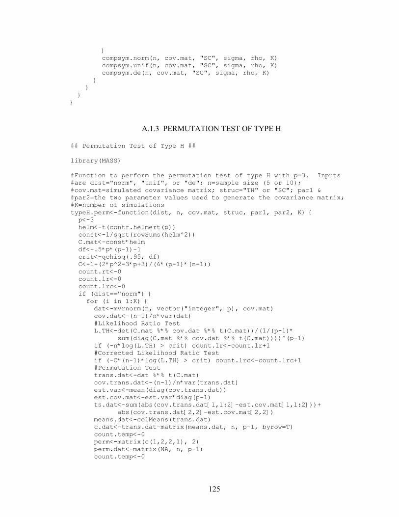
125

}compsym.norm(n, cov.mat, "SC", sigma, rho, K)

compsym.unif(n, cov.mat, "SC", sigma, rho, K) compsym.de(n, cov.mat, "SC", sigma, rho, K) } }

}}

A.1.3 PERMUTATION TEST OF TYPE H

## Permutation Test of Type H ## library(MASS) #Function to perform the permutation test of type H with p=3. Inputs #are dist="norm", "unif", or "de"; n=sample size (5 or 10); #cov.mat=simulated covariance matrix; struc="TH" or "SC"; par1 & #par2=the two parameter values used to generate the covariance matrix; #K=number of simulations typeH.perm<-function(dist, n, cov.mat, struc, par1, par2, K) { p<-3 helm<-t(contr.helmert(p)) const<-1/sqrt(rowSums(helm^2)) C.mat<-const*helm df<-.5*p*(p-1)-1 crit<-qchisq(.95, df) C<-1-(2*p^2-3*p+3)/(6*(p-1)*(n-1)) count.rt<-0 count.lr<-0 count.lrc<-0 if (dist=="norm") { for (i in 1:K) { dat<-mvrnorm(n, vector("integer", p), cov.mat) cov.dat<-(n-1)/n*var(dat) #Likelihood Ratio Test L.TH<-det(C.mat %*% cov.dat %*% t(C.mat))/(1/(p-1)*

sum(diag(C.mat %*% cov.dat %*% t(C.mat))))^(p-1) if (-n*log(L.TH) > crit) count.lr<-count.lr+1 #Corrected Likelihood Ratio Test if (-C*(n-1)*log(L.TH) > crit) count.lrc<-count.lrc+1 #Permutation Test trans.dat<-dat %*% t(C.mat) cov.trans.dat<-(n-1)/n*var(trans.dat) est.var<-mean(diag(cov.trans.dat)) est.cov.mat<-est.var*diag(p-1) ts.dat<-sum(abs(cov.trans.dat[1,1:2]-est.cov.mat[1,1:2]))+

abs(cov.trans.dat[2,2]-est.cov.mat[2,2]) means.dat<-colMeans(trans.dat) c.dat<-trans.dat-matrix(means.dat, n, p-1, byrow=T) count.temp<-0 perm<-matrix(c(1,2,2,1), 2) perm.dat<-matrix(NA, n, p-1) count.temp<-0

126

if (n==5) { for (j1 in 1:2) { for (j2 in 1:2) { for (j3 in 1:2) { for (j4 in 1:2) { for (j5 in 1:2) { perm.dat[1,]<-c(c.dat[1,perm[j1,1]],

c.dat[1,perm[j1,2]]) perm.dat[2,]<-c(c.dat[2,perm[j2,1]],

c.dat[2,perm[j2,2]]) perm.dat[3,]<-c(c.dat[3,perm[j3,1]],

c.dat[3,perm[j3,2]]) perm.dat[4,]<-c(c.dat[4,perm[j4,1]],

c.dat[4,perm[j4,2]]) perm.dat[5,]<-c(c.dat[5,perm[j5,1]],

c.dat[5,perm[j5,2]]) cov.perm<-(n-1)/n*var(perm.dat) ts.perm<-sum(abs(cov.perm[1,1:2]-est.cov.mat[1,1:2]))

+abs(cov.perm[2,2]-est.cov.mat[2,2]) if (ts.perm >= ts.dat) count.temp<-count.temp+1 }

}}

}}if (count.temp/32 < 0.05) count.pt<-count.pt+1

} else { for (j1 in 1:2) { for (j2 in 1:2) { for (j3 in 1:2) { for (j4 in 1:2) { for (j5 in 1:2) { for (j6 in 1:2) { for (j7 in 1:2) { for (j8 in 1:2) { for (j9 in 1:2) { for (j10 in 1:2) { perm.dat[1,]<-c(c.dat[1,perm[j1,1]],

c.dat[1,perm[j1,2]]) perm.dat[2,]<-c(c.dat[2,perm[j2,1]],

c.dat[2,perm[j2,2]]) perm.dat[3,]<-c(c.dat[3,perm[j3,1]],

c.dat[3,perm[j3,2]]) perm.dat[4,]<-c(c.dat[4,perm[j4,1]],

c.dat[4,perm[j4,2]]) perm.dat[5,]<-c(c.dat[5,perm[j5,1]],

c.dat[5,perm[j5,2]]) perm.dat[6,]<-c(c.dat[6,perm[j6,1]],

c.dat[6,perm[j6,2]]) perm.dat[7,]<-c(c.dat[7,perm[j7,1]],

c.dat[7,perm[j7,2]]) perm.dat[8,]<-c(c.dat[8,perm[j8,1]],

c.dat[8,perm[j8,2]]) perm.dat[9,]<-c(c.dat[9,perm[j9,1]],

c.dat[9,perm[j9,2]]) perm.dat[10,]<-c(c.dat[10,perm[j10,1]],

127

c.dat[10,perm[j10,2]]) cov.perm<-(n-1)/n*var(perm.dat) ts.perm<-sum(abs(cov.perm[1,1:2]-

est.cov.mat[1,1:2]))+ abs(cov.perm[2,2]-est.cov.mat[2,2])

if (ts.perm >= ts.dat) count.temp<- count.temp+1

}}

}}

}}

}}

}}if (count.temp/1024 < 0.05) count.pt<-count.pt+1

} }

}if (dist=="unif") {

corr.mat<-cov.mat for (i in 1:p) { for (j in i:p) { corr.mat[i,j]<-2*sin((pi/6)*(cov.mat[i,j]/sqrt(cov.mat[i,i]*

cov.mat[j,j]))) corr.mat[j,i]<-corr.mat[i,j] } }

for (i in 1:K) { unif01.dat<-pnorm(mvrnorm(n, vector("integer", p), corr.mat)) dat<-t(sqrt(12*diag(cov.mat))*t(unif01.dat)) cov.dat<-(n-1)/n*var(dat) #Likelihood Ratio Test L.TH<-det(C.mat %*% cov.dat %*% t(C.mat))/(1/(p-1)*

sum(diag(C.mat %*% cov.dat %*% t(C.mat))))^(p-1) if (-n*log(L.TH) > crit) count.lr<-count.lr+1 #Corrected Likelihood Ratio Test if (-C*(n-1)*log(L.TH) > crit) count.lrc<-count.lrc+1 #Permutation Test trans.dat<-dat %*% t(C.mat) cov.trans.dat<-(n-1)/n*var(trans.dat) est.var<-mean(diag(cov.trans.dat)) est.cov.mat<-est.var*diag(p-1) ts.dat<-sum(abs(cov.trans.dat[1,1:2]-est.cov.mat[1,1:2]))+

abs(cov.trans.dat[2,2]-est.cov.mat[2,2]) means.dat<-colMeans(trans.dat) c.dat<-trans.dat-matrix(means.dat, n, p-1, byrow=T) count.temp<-0 perm<-matrix(c(1,2,2,1), 2) perm.dat<-matrix(NA, n, p-1) count.temp<-0 if (n==5) { for (j1 in 1:2) { for (j2 in 1:2) { for (j3 in 1:2) {

128

for (j4 in 1:2) { for (j5 in 1:2) { perm.dat[1,]<-c(c.dat[1,perm[j1,1]],

c.dat[1,perm[j1,2]]) perm.dat[2,]<-c(c.dat[2,perm[j2,1]],

c.dat[2,perm[j2,2]]) perm.dat[3,]<-c(c.dat[3,perm[j3,1]],

c.dat[3,perm[j3,2]]) perm.dat[4,]<-c(c.dat[4,perm[j4,1]],

c.dat[4,perm[j4,2]]) perm.dat[5,]<-c(c.dat[5,perm[j5,1]],

c.dat[5,perm[j5,2]]) cov.perm<-(n-1)/n*var(perm.dat) ts.perm<-sum(abs(cov.perm[1,1:2]-est.cov.mat[1,1:2]))

+abs(cov.perm[2,2]-est.cov.mat[2,2]) if (ts.perm >= ts.dat) count.temp<-count.temp+1 }

}}

}}if (count.temp/32 < 0.05) count.pt<-count.pt+1

} else { for (j1 in 1:2) { for (j2 in 1:2) { for (j3 in 1:2) { for (j4 in 1:2) { for (j5 in 1:2) { for (j6 in 1:2) { for (j7 in 1:2) { for (j8 in 1:2) { for (j9 in 1:2) { for (j10 in 1:2) { perm.dat[1,]<-c(c.dat[1,perm[j1,1]],

c.dat[1,perm[j1,2]]) perm.dat[2,]<-c(c.dat[2,perm[j2,1]],

c.dat[2,perm[j2,2]]) perm.dat[3,]<-c(c.dat[3,perm[j3,1]],

c.dat[3,perm[j3,2]]) perm.dat[4,]<-c(c.dat[4,perm[j4,1]],

c.dat[4,perm[j4,2]]) perm.dat[5,]<-c(c.dat[5,perm[j5,1]],

c.dat[5,perm[j5,2]]) perm.dat[6,]<-c(c.dat[6,perm[j6,1]],

c.dat[6,perm[j6,2]]) perm.dat[7,]<-c(c.dat[7,perm[j7,1]],

c.dat[7,perm[j7,2]]) perm.dat[8,]<-c(c.dat[8,perm[j8,1]],

c.dat[8,perm[j8,2]]) perm.dat[9,]<-c(c.dat[9,perm[j9,1]],

c.dat[9,perm[j9,2]]) perm.dat[10,]<-c(c.dat[10,perm[j10,1]],

c.dat[10,perm[j10,2]]) cov.perm<-(n-1)/n*var(perm.dat) ts.perm<-sum(abs(cov.perm[1,1:2]-

est.cov.mat[1,1:2]))+

129

abs(cov.perm[2,2]-est.cov.mat[2,2]) if (ts.perm >= ts.dat) count.temp<-

count.temp+1 }

}}

}}

}}

}}

}if (count.temp/1024 < 0.05) count.pt<-count.pt+1

} }

}if (dist=="de") {

b<-0.7824 d<-0.0679 c1<-b^2+6*b*d+9*d^2 c2<-6*d^2 corr.mat<-cov.mat for (i in 1:p) { for (j in i:p) { corr.mat[i,j]<-cov.mat[i,j]/sqrt(cov.mat[i,i]*cov.mat[j,j]) corr.mat[j,i]<-corr.mat[i,j] } }

corr.int<-corr.mat for (j in 1:(p-1)) { for (k in (j+1):p) { corr.int[j,k]<-Re(polyroot(c(-corr.mat[j,k],c1,0,c2))[1]) corr.int[k,j]<-corr.int[j,k] } }

for (i in 1:K) { norm.dat<-mvrnorm(n, vector("integer", p), corr.int) dat<-t(sqrt(diag(cov.mat))*t(b*norm.dat+d*norm.dat^3)) cov.dat<-(n-1)/n*var(dat) #Likelihood Ratio Test L.TH<-det(C.mat %*% cov.dat %*% t(C.mat))/(1/(p-1)*

sum(diag(C.mat %*% cov.dat %*% t(C.mat))))^(p-1) if (-n*log(L.TH) > crit) count.lr<-count.lr+1 #Corrected Likelihood Ratio Test if (-C*(n-1)*log(L.TH) > crit) count.lrc<-count.lrc+1 #Permutation Test trans.dat<-dat %*% t(C.mat) cov.trans.dat<-(n-1)/n*var(trans.dat) est.var<-mean(diag(cov.trans.dat)) est.cov.mat<-est.var*diag(p-1) ts.dat<-sum(abs(cov.trans.dat[1,1:2]-est.cov.mat[1,1:2]))+

abs(cov.trans.dat[2,2]-est.cov.mat[2,2]) means.dat<-colMeans(trans.dat) c.dat<-trans.dat-matrix(means.dat, n, p-1, byrow=T) count.temp<-0 perm<-matrix(c(1,2,2,1), 2)

130

perm.dat<-matrix(NA, n, p-1) count.temp<-0 if (n==5) { for (j1 in 1:2) { for (j2 in 1:2) { for (j3 in 1:2) { for (j4 in 1:2) { for (j5 in 1:2) { perm.dat[1,]<-c(c.dat[1,perm[j1,1]],

c.dat[1,perm[j1,2]]) perm.dat[2,]<-c(c.dat[2,perm[j2,1]],

c.dat[2,perm[j2,2]]) perm.dat[3,]<-c(c.dat[3,perm[j3,1]],

c.dat[3,perm[j3,2]]) perm.dat[4,]<-c(c.dat[4,perm[j4,1]],

c.dat[4,perm[j4,2]]) perm.dat[5,]<-c(c.dat[5,perm[j5,1]],

c.dat[5,perm[j5,2]]) cov.perm<-(n-1)/n*var(perm.dat) ts.perm<-sum(abs(cov.perm[1,1:2]-est.cov.mat[1,1:2]))

+abs(cov.perm[2,2]-est.cov.mat[2,2]) if (ts.perm >= ts.dat) count.temp<-count.temp+1 }

}}

}}if (count.temp/32 < 0.05) count.pt<-count.pt+1

} else { for (j1 in 1:2) { for (j2 in 1:2) { for (j3 in 1:2) { for (j4 in 1:2) { for (j5 in 1:2) { for (j6 in 1:2) { for (j7 in 1:2) { for (j8 in 1:2) { for (j9 in 1:2) { for (j10 in 1:2) { perm.dat[1,]<-c(c.dat[1,perm[j1,1]],

c.dat[1,perm[j1,2]]) perm.dat[2,]<-c(c.dat[2,perm[j2,1]],

c.dat[2,perm[j2,2]]) perm.dat[3,]<-c(c.dat[3,perm[j3,1]],

c.dat[3,perm[j3,2]]) perm.dat[4,]<-c(c.dat[4,perm[j4,1]],

c.dat[4,perm[j4,2]]) perm.dat[5,]<-c(c.dat[5,perm[j5,1]],

c.dat[5,perm[j5,2]]) perm.dat[6,]<-c(c.dat[6,perm[j6,1]],

c.dat[6,perm[j6,2]]) perm.dat[7,]<-c(c.dat[7,perm[j7,1]],

c.dat[7,perm[j7,2]]) perm.dat[8,]<-c(c.dat[8,perm[j8,1]],

c.dat[8,perm[j8,2]]) perm.dat[9,]<-c(c.dat[9,perm[j9,1]],

131

c.dat[9,perm[j9,2]]) perm.dat[10,]<-c(c.dat[10,perm[j10,1]],

c.dat[10,perm[j10,2]]) cov.perm<-(n-1)/n*var(perm.dat) ts.perm<-sum(abs(cov.perm[1,1:2]-

est.cov.mat[1,1:2]))+ abs(cov.perm[2,2]-est.cov.mat[2,2])

if (ts.perm >= ts.dat) count.temp<- count.temp+1

}}

}}

}}

}}

}}if (count.temp/1024 < 0.05) count.pt<-count.pt+1

} }

}p.values<-c(count.pt/K, count.lr/K, count.lrc/K)

write(c(struc, dist, n, p, par1, par2, p.values), "Type H", 9, TRUE, "\t") }K<-1000 #Type I Error for (n in c(5, 10)) { for (lambda in c(2, 3, 4)) { for (diff in c(lambda-1, lambda, lambda+1)) { cov.mat<-diag(seq(1, (p-1)*diff+1, by=diff)) for (i in 1:(p-1)) { for (j in (i+1):p) { cov.mat[i,j]<-0.5*(cov.mat[i,i]+cov.mat[j,j])-lambda cov.mat[j,i]<-cov.mat[i,j] }

}typeH.perm("norm", n, cov.mat, "TH", lambda, diff, K)

typeH.perm("unif", n, cov.mat, "TH", lambda, diff, K) typeH.perm("de", n, cov.mat, "TH", lambda, diff, K) }

}}#Power vs. Serial Correlation p<-3 for (n in c(5, 10)) { for (sigma in c(1, 3, 5)) { for (rho in c(0.3, 0.6, 0.9)) { cov.mat<-(sigma^2/(1-rho^2))*diag(p) for (i in 1:(p-1)) { for (j in (i+1):p) { cov.mat[i,j]<-(sigma^2/(1-rho^2))*rho^(j-i) cov.mat[j,i]<-cov.mat[i,j] }

}

132

typeH.perm("norm", n, cov.mat, "SC", sigma, rho, K) typeH.perm("unif", n, cov.mat, "SC", sigma, rho, K) typeH.perm("de", n, cov.mat, "SC", sigma, rho, K) }

}}

A.1.4 RANDOMIZATION TEST OF TYPE H STRUCTURE

## Randomization Test of Type H ## library(MASS) #Function to perform the test of type H with multivariate normal data. #Inputs are n=sample size; cov.mat=simulated covariance matrix; #struc="TH" or "SC"; par1 & par2=the two parameter values used to #generate the covariance matrix; K=number of simulations typeH.norm<-function(n, cov.mat, struc, par1, par2, K) { dist<-"norm" p<-dim(cov.mat)[1] helm<-t(contr.helmert(p)) const<-1/sqrt(rowSums(helm^2)) C.mat<-const*helm df<-.5*p*(p-1)-1 crit<-qchisq(.95, df) C<-1-(2*p^2-3*p+3)/(6*(p-1)*(n-1)) perm<-matrix(NA, n, p) count.rt<-0 count.lr<-0 count.lrc<-0 if (n>p) { for (i in 1:K) { dat<-mvrnorm(n, vector("integer", p), cov.mat)

cov.dat<-(n-1)/n*var(dat) #Likelihood Ratio Test L.TH<-det(C.mat %*% cov.dat %*% t(C.mat))/(1/(p-1)*

sum(diag(C.mat %*% cov.dat %*% t(C.mat))))^(p-1) if (-n*log(L.TH) > crit) count.lr<-count.lr+1 #Corrected Likelihood Ratio Test if (-C*(n-1)*log(L.TH) > crit) count.lrc<-count.lrc+1 #Randomization Test trans.dat<-dat %*% t(C.mat) cov.trans.dat<-(n-1)/n*var(trans.dat) est.var<-mean(diag(cov.trans.dat)) est.cov.mat<-est.var*diag(p-1) ts.dat<-0 for (j in 1:(p-1)) { ts.dat<-ts.dat+sum(abs(cov.trans.dat[j,j:(p-1)]-

est.cov.mat[j,j:(p-1)])) } means.dat<-colMeans(trans.dat) c.dat<-trans.dat-matrix(means.dat, n, p-1, byrow=T) count.temp<-0 for (j in 1:1000) { perm<-t(apply(c.dat, 1, sample))

133

cov.perm<-(n-1)/n*var(perm) ts.perm<-0 for (k in 1:(p-1)) { ts.perm<-ts.perm+sum(abs(cov.perm[k,k:(p-1)]-

est.cov.mat[k,k:(p-1)])) }

if (ts.perm >= ts.dat) count.temp<-count.temp+1 } if (count.temp/1000 < 0.05) count.rt<-count.rt+1 }

p.values<-c(count.rt/K, count.lr/K, count.lrc/K) write(c(struc, dist, n, p, par1, par2, p.values), "Type H", 9, TRUE, "\t") }

else { for (i in 1:K) { dat<-mvrnorm(n, vector("integer", p), cov.mat) #Randomization Test trans.dat<-dat %*% t(C.mat) cov.trans.dat<-(n-1)/n*var(trans.dat) est.var<-mean(diag(cov.trans.dat)) est.cov.mat<-est.var*diag(p-1) ts.dat<-0 for (j in 1:(p-1)) { ts.dat<-ts.dat+sum(abs(cov.trans.dat[j,j:(p-1)]-

est.cov.mat[j,j:(p-1)])) } means.dat<-colMeans(trans.dat) c.dat<-trans.dat-matrix(means.dat, n, p-1, byrow=T) count.temp<-0 for (j in 1:1000) { perm<-t(apply(c.dat, 1, sample)) cov.perm<-(n-1)/n*var(perm) ts.perm<-0 for (k in 1:(p-1)) { ts.perm<-ts.perm+sum(abs(cov.perm[k,k:(p-1)]-

est.cov.mat[k,k:(p-1)])) }

if (ts.perm >= ts.dat) count.temp<-count.temp+1 } if (count.temp/1000 < 0.05) count.rt<-count.rt+1 }

p.values<-c(count.rt/K, "NA", "NA") write(c(struc, dist, n, p, par1, par2, p.values), "Type H", 9, TRUE, "\t") }}

#Function to perform the test of type H with multivariate uniform data. #Inputs are n=sample size; cov.mat=simulated covariance matrix; #struc="TH" or "SC"; par1 & par2=the two parameter values used to #generate the covariance matrix; K=number of simulations typeH.unif<-function(n, cov.mat, struc, par1, par2, K) { dist<-"unif" p<-dim(cov.mat)[1] helm<-t(contr.helmert(p)) const<-1/sqrt(rowSums(helm^2))

134

C.mat<-const*helm df<-.5*p*(p-1)-1 crit<-qchisq(.95, df) C<-1-(2*p^2-3*p+3)/(6*(p-1)*(n-1)) perm<-matrix(NA, n, p) count.rt<-0 count.lr<-0 count.lrc<-0 corr.mat<-cov.mat for (i in 1:p) { for (j in i:p) { corr.mat[i,j]<-2*sin((pi/6)*(cov.mat[i,j]/sqrt(cov.mat[i,i]*

cov.mat[j,j]))) corr.mat[j,i]<-corr.mat[i,j] }

}if (n>p) {

for (i in 1:K) { unif01.dat<-pnorm(mvrnorm(n, vector("integer", p), corr.mat)) dat<-t(sqrt(12*diag(cov.mat))*t(unif01.dat)) cov.dat<-(n-1)/n*var(dat) #Likelihood Ratio Test L.TH<-det(C.mat %*% cov.dat %*% t(C.mat))/(1/(p-1)*

sum(diag(C.mat %*% cov.dat %*% t(C.mat))))^(p-1) if (-n*log(L.TH) > crit) count.lr<-count.lr+1 #Corrected Likelihood Ratio Test if (-C*(n-1)*log(L.TH) > crit) count.lrc<-count.lrc+1 #Randomization Test trans.dat<-dat %*% t(C.mat) cov.trans.dat<-(n-1)/n*var(trans.dat) est.var<-mean(diag(cov.trans.dat)) est.cov.mat<-est.var*diag(p-1) ts.dat<-0 for (j in 1:(p-1)) { ts.dat<-ts.dat+sum(abs(cov.trans.dat[j,j:(p-1)]-

est.cov.mat[j,j:(p-1)])) } means.dat<-colMeans(trans.dat) c.dat<-trans.dat-matrix(means.dat, n, p-1, byrow=T) count.temp<-0 for (j in 1:1000) { perm<-t(apply(c.dat, 1, sample)) cov.perm<-(n-1)/n*var(perm) ts.perm<-0 for (k in 1:(p-1)) { ts.perm<-ts.perm+sum(abs(cov.perm[k,k:(p-1)]-

est.cov.mat[k,k:(p-1)])) }

if (ts.perm >= ts.dat) count.temp<-count.temp+1 } if (count.temp/1000 < 0.05) count.rt<-count.rt+1 }

p.values<-c(count.rt/K, count.lr/K, count.lrc/K) write(c(struc, dist, n, p, par1, par2, p.values), "Type H", 9, TRUE, "\t") }

else {

135

for (i in 1:K) { unif01.dat<-pnorm(mvrnorm(n, vector("integer", p), corr.mat)) dat<-t(sqrt(12*diag(cov.mat))*t(unif01.dat)) #Randomization Test trans.dat<-dat %*% t(C.mat) cov.trans.dat<-(n-1)/n*var(trans.dat) est.var<-mean(diag(cov.trans.dat)) est.cov.mat<-est.var*diag(p-1) ts.dat<-0 for (j in 1:(p-1)) { ts.dat<-ts.dat+sum(abs(cov.trans.dat[j,j:(p-1)]-

est.cov.mat[j,j:(p-1)])) } means.dat<-colMeans(trans.dat) c.dat<-trans.dat-matrix(means.dat, n, p-1, byrow=T) count.temp<-0 for (j in 1:1000) { perm<-t(apply(c.dat, 1, sample)) cov.perm<-(n-1)/n*var(perm) ts.perm<-0 for (k in 1:(p-1)) { ts.perm<-ts.perm+sum(abs(cov.perm[k,k:(p-1)]-

est.cov.mat[k,k:(p-1)])) }

if (ts.perm >= ts.dat) count.temp<-count.temp+1 } if (count.temp/1000 < 0.05) count.rt<-count.rt+1 }

p.values<-c(count.rt/K, "NA", "NA") write(c(struc, dist, n, p, par1, par2, p.values), "Type H", 9, TRUE, "\t") }}

#Function to perform the test of type H with multivariate double #exponential data. Inputs are n=sample size; cov.mat=simulated #covariance matrix; struc="TH" or "SC"; par1 & par2=the two parameter #values used to generate the covariance matrix; K=number of simulations typeH.de<-function(n, cov.mat, struc, par1, par2, K) { dist<-"de" p<-dim(cov.mat)[1] helm<-t(contr.helmert(p)) const<-1/sqrt(rowSums(helm^2)) C.mat<-const*helm b<-0.7824 d<-0.0679 c1<-b^2+6*b*d+9*d^2 c2<-6*d^2 df<-.5*p*(p-1)-1 crit<-qchisq(.95, df) C<-1-(2*p^2-3*p+3)/(6*(p-1)*(n-1)) perm<-matrix(NA, n, p) count.rt<-0 count.lr<-0 count.lrc<-0 corr.mat<-cov.mat for (i in 1:p) {

136

for (j in i:p) { corr.mat[i,j]<-cov.mat[i,j]/sqrt(cov.mat[i,i]*cov.mat[j,j]) corr.mat[j,i]<-corr.mat[i,j] }

}corr.int<-corr.mat

for (j in 1:(p-1)) { for (k in (j+1):p) { corr.int[j,k]<-Re(polyroot(c(-corr.mat[j,k],c1,0,c2))[1]) corr.int[k,j]<-corr.int[j,k] }

}if (n>p) {

for (i in 1:K) { norm.dat<-mvrnorm(n, vector("integer", p), corr.int) dat<-t(sqrt(diag(cov.mat))*t(b*norm.dat+d*norm.dat^3)) cov.dat<-(n-1)/n*var(dat) #Likelihood Ratio Test L.TH<-det(C.mat %*% cov.dat %*% t(C.mat))/(1/(p-1)*

sum(diag(C.mat %*% cov.dat %*% t(C.mat))))^(p-1) if (-n*log(L.TH) > crit) count.lr<-count.lr+1 #Corrected Likelihood Ratio Test if (-C*(n-1)*log(L.TH) > crit) count.lrc<-count.lrc+1 #Randomization Test trans.dat<-dat %*% t(C.mat) cov.trans.dat<-(n-1)/n*var(trans.dat) est.var<-mean(diag(cov.trans.dat)) est.cov.mat<-est.var*diag(p-1) ts.dat<-0 for (j in 1:(p-1)) { ts.dat<-ts.dat+sum(abs(cov.trans.dat[j,j:(p-1)]-

est.cov.mat[j,j:(p-1)])) } means.dat<-colMeans(trans.dat) c.dat<-trans.dat-matrix(means.dat, n, p-1, byrow=T) count.temp<-0 for (j in 1:1000) { perm<-t(apply(c.dat, 1, sample)) cov.perm<-(n-1)/n*var(perm) ts.perm<-0 for (k in 1:(p-1)) { ts.perm<-ts.perm+sum(abs(cov.perm[k,k:(p-1)]-

est.cov.mat[k,k:(p-1)])) }

if (ts.perm >= ts.dat) count.temp<-count.temp+1 } if (count.temp/1000 < 0.05) count.rt<-count.rt+1 }

p.values<-c(count.rt/K, count.lr/K, count.lrc/K) write(c(struc, dist, n, p, par1, par2, p.values), "Type H", 9, TRUE, "\t") }

else { for (i in 1:K) { norm.dat<-mvrnorm(n, vector("integer", p), cov.int) dat<-t(sqrt(diag(cov.mat))*t(b*norm.dat+d*norm.dat^3)) #Randomization Test

137

trans.dat<-dat %*% t(C.mat) cov.trans.dat<-(n-1)/n*var(trans.dat) est.var<-mean(diag(cov.trans.dat)) est.cov.mat<-est.var*diag(p-1) ts.dat<-0 for (j in 1:(p-1)) { ts.dat<-ts.dat+sum(abs(cov.trans.dat[j,j:(p-1)]-

est.cov.mat[j,j:(p-1)])) } means.dat<-colMeans(trans.dat) c.dat<-trans.dat-matrix(means.dat, n, p-1, byrow=T) count.temp<-0 for (j in 1:1000) { perm<-t(apply(c.dat, 1, sample)) cov.perm<-(n-1)/n*var(perm) ts.perm<-0 for (k in 1:(p-1)) { ts.perm<-ts.perm+sum(abs(cov.perm[k,k:(p-1)]-

est.cov.mat[k,k:(p-1)])) }

if (ts.perm >= ts.dat) count.temp<-count.temp+1 } if (count.temp/1000 < 0.05) count.rt<-count.rt+1 }

p.values<-c(count.rt/K, "NA", "NA") write(c(struc, dist, n, p, par1, par2, p.values), "Type H", 9, TRUE, "\t") }}K<-1000 #Type I Error n<-25 p<-3 for (lambda in c(2, 3, 4)) { for (diff in c(lambda-1, lambda, lambda+1)) { cov.mat<-diag(seq(1, (p-1)*diff+1, by=diff)) for (i in 1:(p-1)) { for (j in (i+1):p) { cov.mat[i,j]<-0.5*(cov.mat[i,i]+cov.mat[j,j])-lambda cov.mat[j,i]<-cov.mat[i,j] } }

typeH.norm(n, cov.mat, "TH", lambda, diff, K) typeH.unif(n, cov.mat, "TH", lambda, diff, K) typeH.de(n, cov.mat, "TH", lambda, diff, K) }}p<-5 for (n in c(5, 10, 25)) { for (lambda in c(1.25, 1.5)) { for (diff in c(2*lambda/5-.4, 2*lambda/5, 2*lambda/5+.4)) { cov.mat<-diag(seq(1, (p-1)*diff+1, by=diff)) for (i in 1:(p-1)) { for (j in (i+1):p) { cov.mat[i,j]<-0.5*(cov.mat[i,i]+cov.mat[j,j])-lambda cov.mat[j,i]<-cov.mat[i,j] }

138

}typeH.norm(n, cov.mat, "TH", lambda, diff, K)

typeH.unif(n, cov.mat, "TH", lambda, diff, K) typeH.de(n, cov.mat, "TH", lambda, diff, K) }

}}lambda<-1 for (n in c(5, 10, 25)) { for (diff in c(0.1, 0.4, 0.8)) { cov.mat<-diag(seq(1, (p-1)*diff+1, by=diff)) for (i in 1:(p-1)) { for (j in (i+1):p) { cov.mat[i,j]<-0.5*(cov.mat[i,i]+cov.mat[j,j])-lambda cov.mat[j,i]<-cov.mat[i,j]

}}typeH.norm(n, cov.mat, "TH", lambda, diff, K)

typeH.unif(n, cov.mat, "TH", lambda, diff, K) typeH.de(n, cov.mat, "TH", lambda, diff, K) }}p<-10 for (n in c(5, 10, 25)) { for (lambda in c(0.5, 0.75, 1)) { for (diff in c(.1, .1+(2*lambda+1)/50, .1+(2*lambda+1)/25)) { cov.mat<-diag(seq(1, (p-1)*diff+1, by=diff)) for (i in 1:(p-1)) { for (j in (i+1):p) { cov.mat[i,j]<-0.5*(cov.mat[i,i]+cov.mat[j,j])-lambda cov.mat[j,i]<-cov.mat[i,j] }

}typeH.norm(n, cov.mat, "TH", lambda, diff, K)

typeH.unif(n, cov.mat, "TH", lambda, diff, K) typeH.de(n, cov.mat, "TH", lambda, diff, K) }

}}#Power vs. Serial Correlation n<-25 p<-3 for (sigma in c(1, 3, 5)) { for (rho in c(0.3, 0.6, 0.9)) { cov.mat<-(sigma^2/(1-rho^2))*diag(p) for (i in 1:(p-1)) { for (j in (i+1):p) { cov.mat[i,j]<-(sigma^2/(1-rho^2))*rho^(j-i) cov.mat[j,i]<-cov.mat[i,j] } }

typeH.norm(n, cov.mat, "SC", sigma, rho, K) typeH.unif(n, cov.mat, "SC", sigma, rho, K) typeH.de(n, cov.mat, "SC", sigma, rho, K) }}for (n in c(5, 10, 25)) {

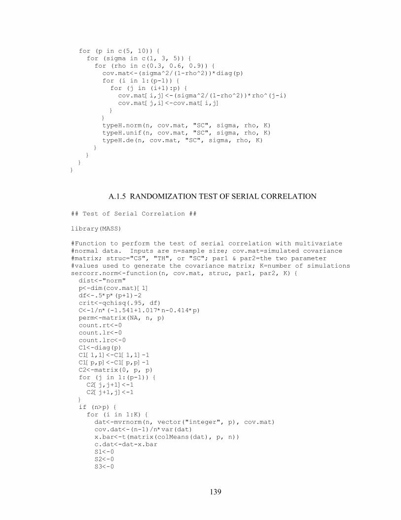
139

for (p in c(5, 10)) { for (sigma in c(1, 3, 5)) { for (rho in c(0.3, 0.6, 0.9)) { cov.mat<-(sigma^2/(1-rho^2))*diag(p) for (i in 1:(p-1)) { for (j in (i+1):p) { cov.mat[i,j]<-(sigma^2/(1-rho^2))*rho^(j-i) cov.mat[j,i]<-cov.mat[i,j] }

}typeH.norm(n, cov.mat, "SC", sigma, rho, K)

typeH.unif(n, cov.mat, "SC", sigma, rho, K) typeH.de(n, cov.mat, "SC", sigma, rho, K) } }

}}

A.1.5 RANDOMIZATION TEST OF SERIAL CORRELATION

## Test of Serial Correlation ## library(MASS) #Function to perform the test of serial correlation with multivariate #normal data. Inputs are n=sample size; cov.mat=simulated covariance #matrix; struc="CS", "TH", or "SC"; par1 & par2=the two parameter #values used to generate the covariance matrix; K=number of simulations sercorr.norm<-function(n, cov.mat, struc, par1, par2, K) { dist<-"norm" p<-dim(cov.mat)[1] df<-.5*p*(p+1)-2 crit<-qchisq(.95, df) C<-1/n*(-1.541+1.017*n-0.414*p) perm<-matrix(NA, n, p) count.rt<-0 count.lr<-0 count.lrc<-0 C1<-diag(p) C1[1,1]<-C1[1,1]-1 C1[p,p]<-C1[p,p]-1 C2<-matrix(0, p, p) for (j in 1:(p-1)) { C2[j,j+1]<-1 C2[j+1,j]<-1 }

if (n>p) { for (i in 1:K) { dat<-mvrnorm(n, vector("integer", p), cov.mat) cov.dat<-(n-1)/n*var(dat) x.bar<-t(matrix(colMeans(dat), p, n)) c.dat<-dat-x.bar S1<-0 S2<-0 S3<-0

140

for (j in 1:n) { S1<-S1+t(c.dat[j,])%*%C1%*%c.dat[j,] S2<-S2+t(c.dat[j,])%*%C2%*%c.dat[j,] S3<-S3+t(c.dat[j,])%*%c.dat[j,] } func<-function(rho.hat) -2*S1*(1-p)*rho.hat^3+S2*(2-p)*rho.hat^2-

2*(S1*p+S3)*rho.hat+S2*p rho.hat<-uniroot(func, low=-1, up=1)$root sig2.hat<-as.numeric(1/(n*p)*(S1*rho.hat^2-S2*rho.hat+S3)) #Likelihood Ratio Test L.SC<-det(cov.dat)/(sig2.hat^p/(1-rho.hat^2)) if (-n*log(L.SC) > crit) count.lr<-count.lr+1 #Corrected Likelihood Ratio Test if (-C*n*log(L.SC) > crit) count.lrc<-count.lrc+1 #Randomization Test est.cov.mat<-sig2.hat/(1-rho.hat^2)*matrix(1, p, p) for (j in 1:(p-1)) { for (k in (j+1):p) { est.cov.mat[j,k]<-est.cov.mat[j,k]*rho.hat^(k-j) est.cov.mat[k,j]<-est.cov.mat[j,k] }

}eigen.vec<-eigen(est.cov.mat)$vectors

eigen.val<-eigen(est.cov.mat)$values trans.dat<-c.dat%*%eigen.vec for (j in 1:p) { trans.dat[,j]<-trans.dat[,j]/sqrt(eigen.val[j]) } cov.trans.dat<-(n-1)/n*var(trans.dat) est.cov.mat<-diag(p) ts.dat<-0 for (j in 1:p) { ts.dat<-ts.dat+sum(abs(cov.trans.dat[j,j:p]-

est.cov.mat[j,j:p])) } count.temp<-0 for (j in 1:1000) { perm<-t(apply(trans.dat, 1, sample)) cov.perm<-(n-1)/n*var(perm) ts.perm<-0 for (k in 1:p) { ts.perm<-ts.perm+sum(abs(cov.perm[k,k:p]-est.cov.mat[k,k:p])) }

if (ts.perm >= ts.dat) count.temp<-count.temp+1 } if (count.temp/1000 < 0.05) count.rt<-count.rt+1 }

p.values<-c(count.rt/K, count.lr/K, count.lrc/K) write(c(struc, dist, n, p, par1, par2, p.values), "Serial Correlation", 9, TRUE, "\t") }

else { for (i in 1:K) { dat<-mvrnorm(n, vector("integer", p), cov.mat) x.bar<-t(matrix(colMeans(dat), p, n)) c.dat<-dat-x.bar S1<-0

141

S2<-0 S3<-0 for (j in 1:n) { S1<-S1+t(c.dat[j,])%*%C1%*%c.dat[j,] S2<-S2+t(c.dat[j,])%*%C2%*%c.dat[j,] S3<-S3+t(c.dat[j,])%*%c.dat[j,] } func<-function(rho.hat) -2*S1*(1-p)*rho.hat^3+S2*(2-p)*rho.hat^2-

2*(S1*p+S3)*rho.hat+S2*p rho.hat<-uniroot(func, low=-1, up=1)$root sig2.hat<-as.numeric(1/(n*p)*(S1*rho.hat^2-S2*rho.hat+S3)) #Randomization Test est.cov.mat<-sig2.hat/(1-rho.hat^2)*matrix(1, p, p) for (j in 1:(p-1)) { for (k in (j+1):p) { est.cov.mat[j,k]<-est.cov.mat[j,k]*rho.hat^(k-j) est.cov.mat[k,j]<-est.cov.mat[j,k] }

}eigen.vec<-eigen(est.cov.mat)$vectors

eigen.val<-eigen(est.cov.mat)$values trans.dat<-c.dat%*%eigen.vec for (j in 1:p) { trans.dat[,j]<-trans.dat[,j]/sqrt(eigen.val[j]) } cov.trans.dat<-(n-1)/n*var(trans.dat) est.cov.mat<-diag(p) ts.dat<-0 for (j in 1:p) { ts.dat<-ts.dat+sum(abs(cov.trans.dat[j,j:p]-

est.cov.mat[j,j:p])) } count.temp<-0 for (j in 1:1000) { perm<-t(apply(trans.dat, 1, sample)) cov.perm<-(n-1)/n*var(perm) ts.perm<-0 for (k in 1:p) { ts.perm<-ts.perm+sum(abs(cov.perm[k,k:p]-est.cov.mat[k,k:p])) }

if (ts.perm >= ts.dat) count.temp<-count.temp+1 } if (count.temp/1000 < 0.05) count.rt<-count.rt+1 }

p.values<-c(count.rt/K, "NA", "NA") write(c(struc, dist, n, p, par1, par2, p.values), "Serial Correlation", 9, TRUE, "\t") }}

#Function to perform the test of serial correlation with multivariate #uniform data. Inputs are n=sample size; cov.mat=simulated covariance #matrix; struc="CS", "TH", or "SC"; par1 & par2=the two parameter #values used to generate the covariance matrix; K=number of simulations sercorr.unif<-function(n, cov.mat, struc, par1, par2, K) { dist<-"unif" p<-dim(cov.mat)[1]

142

df<-.5*p*(p+1)-2 crit<-qchisq(.95, df) C<-1/n*(-1.541+1.017*n-0.414*p) perm<-matrix(NA, n, p) count.rt<-0 count.lr<-0 count.lrc<-0 C1<-diag(p) C1[1,1]<-C1[1,1]-1 C1[p,p]<-C1[p,p]-1 C2<-matrix(0, p, p) for (j in 1:(p-1)) { C2[j,j+1]<-1 C2[j+1,j]<-1 }

corr.mat<-cov.mat for (i in 1:p) { for (j in i:p) { corr.mat[i,j]<-2*sin((pi/6)*(cov.mat[i,j]/sqrt(cov.mat[i,i]*

cov.mat[j,j]))) corr.mat[j,i]<-corr.mat[i,j] }

}if (n>p) {

for (i in 1:K) { unif01.dat<-pnorm(mvrnorm(n, vector("integer", p), corr.mat)) dat<-t(sqrt(12*diag(cov.mat))*t(unif01.dat)) cov.dat<-(n-1)/n*var(dat) x.bar<-t(matrix(colMeans(dat), p, n)) c.dat<-dat-x.bar S1<-0 S2<-0 S3<-0 for (j in 1:n) { S1<-S1+t(c.dat[j,])%*%C1%*%c.dat[j,] S2<-S2+t(c.dat[j,])%*%C2%*%c.dat[j,] S3<-S3+t(c.dat[j,])%*%c.dat[j,] } func<-function(rho.hat) -2*S1*(1-p)*rho.hat^3+S2*(2-p)*rho.hat^2-

2*(S1*p+S3)*rho.hat+S2*p rho.hat<-uniroot(func, low=-1, up=1)$root sig2.hat<-as.numeric(1/(n*p)*(S1*rho.hat^2-S2*rho.hat+S3)) #Likelihood Ratio Test L.SC<-det(cov.dat)/(sig2.hat^p/(1-rho.hat^2)) if (-n*log(L.SC) > crit) count.lr<-count.lr+1 #Corrected Likelihood Ratio Test if (-C*n*log(L.SC) > crit) count.lrc<-count.lrc+1 #Randomization Test est.cov.mat<-sig2.hat/(1-rho.hat^2)*matrix(1, p, p) for (j in 1:(p-1)) { for (k in (j+1):p) { est.cov.mat[j,k]<-est.cov.mat[j,k]*rho.hat^(k-j) est.cov.mat[k,j]<-est.cov.mat[j,k] }

}eigen.vec<-eigen(est.cov.mat)$vectors

eigen.val<-eigen(est.cov.mat)$values

143

trans.dat<-c.dat%*%eigen.vec for (j in 1:p) { trans.dat[,j]<-trans.dat[,j]/sqrt(eigen.val[j]) } cov.trans.dat<-(n-1)/n*var(trans.dat) est.cov.mat<-diag(p) ts.dat<-0 for (j in 1:p) { ts.dat<-ts.dat+sum(abs(cov.trans.dat[j,j:p]-

est.cov.mat[j,j:p])) } count.temp<-0 for (j in 1:1000) { perm<-t(apply(trans.dat, 1, sample)) cov.perm<-(n-1)/n*var(perm) ts.perm<-0 for (k in 1:p) { ts.perm<-ts.perm+sum(abs(cov.perm[k,k:p]-est.cov.mat[k,k:p])) }

if (ts.perm >= ts.dat) count.temp<-count.temp+1 } if (count.temp/1000 < 0.05) count.rt<-count.rt+1 }

p.values<-c(count.rt/K, count.lr/K, count.lrc/K) write(c(struc, dist, n, p, par1, par2, p.values), "Serial Correlation", 9, TRUE, "\t") }

else { for (i in 1:K) { unif01.dat<-pnorm(mvrnorm(n, vector("integer", p), corr.mat)) dat<-t(sqrt(12*diag(cov.mat))*t(unif01.dat)) x.bar<-t(matrix(colMeans(dat), p, n)) c.dat<-dat-x.bar S1<-0 S2<-0 S3<-0 for (j in 1:n) { S1<-S1+t(c.dat[j,])%*%C1%*%c.dat[j,] S2<-S2+t(c.dat[j,])%*%C2%*%c.dat[j,] S3<-S3+t(c.dat[j,])%*%c.dat[j,] } func<-function(rho.hat) -2*S1*(1-p)*rho.hat^3+S2*(2-p)*rho.hat^2-

2*(S1*p+S3)*rho.hat+S2*p rho.hat<-uniroot(func, low=-1, up=1)$root sig2.hat<-as.numeric(1/(n*p)*(S1*rho.hat^2-S2*rho.hat+S3)) #Randomization Test est.cov.mat<-sig2.hat/(1-rho.hat^2)*matrix(1, p, p) for (j in 1:(p-1)) { for (k in (j+1):p) { est.cov.mat[j,k]<-est.cov.mat[j,k]*rho.hat^(k-j) est.cov.mat[k,j]<-est.cov.mat[j,k] }

}eigen.vec<-eigen(est.cov.mat)$vectors

eigen.val<-eigen(est.cov.mat)$values trans.dat<-c.dat%*%eigen.vec for (j in 1:p) {

144

trans.dat[,j]<-trans.dat[,j]/sqrt(eigen.val[j]) } cov.trans.dat<-(n-1)/n*var(trans.dat) est.cov.mat<-diag(p) ts.dat<-0 for (j in 1:p) { ts.dat<-ts.dat+sum(abs(cov.trans.dat[j,j:p]-

est.cov.mat[j,j:p])) } count.temp<-0 for (j in 1:1000) { perm<-t(apply(trans.dat, 1, sample)) cov.perm<-(n-1)/n*var(perm) ts.perm<-0 for (k in 1:p) { ts.perm<-ts.perm+sum(abs(cov.perm[k,k:p]-est.cov.mat[k,k:p])) }

if (ts.perm >= ts.dat) count.temp<-count.temp+1 }

if (count.temp/1000 < 0.05) count.rt<-count.rt+1 }

p.values<-c(count.rt/K, "NA", "NA") write(c(struc, dist, n, p, par1, par2, p.values), "Serial Correlation", 9, TRUE, "\t") }}

#Function to perform the test of serial correlation with multivariate #double exponential data. Inputs are n=sample size; cov.mat=simulated #covariance matrix; struc="CS", "TH", or "SC"; par1 & par2=the two #parameter values used to generate the covariance matrix; K=number of #simulations sercorr.de<-function(n, cov.mat, struc, par1, par2, K) { dist<-"de" p<-dim(cov.mat)[1] b<-0.7824 d<-0.0679 c1<-b^2+6*b*d+9*d^2 c2<-6*d^2 df<-.5*p*(p+1)-2 crit<-qchisq(.95, df) C<-1/n*(-1.541+1.017*n-0.414*p) perm<-matrix(NA, n, p) count.rt<-0 count.lr<-0 count.lrc<-0 C1<-diag(p) C1[1,1]<-C1[1,1]-1 C1[p,p]<-C1[p,p]-1 C2<-matrix(0, p, p) for (j in 1:(p-1)) { C2[j,j+1]<-1 C2[j+1,j]<-1 }

corr.mat<-cov.mat for (i in 1:p) { for (j in i:p) {

145

corr.mat[i,j]<-cov.mat[i,j]/sqrt(cov.mat[i,i]*cov.mat[j,j]) corr.mat[j,i]<-corr.mat[i,j] }

}corr.int<-corr.mat

for (j in 1:(p-1)) { for (k in (j+1):p) { corr.int[j,k]<-Re(polyroot(c(-corr.mat[j,k],c1,0,c2))[1]) corr.int[k,j]<-corr.int[j,k] }

}if (n>p) {

for (i in 1:K) { norm.dat<-mvrnorm(n, vector("integer", p), corr.int) dat<-t(sqrt(diag(cov.mat))*t(b*norm.dat+d*norm.dat^3)) cov.dat<-(n-1)/n*var(dat) x.bar<-t(matrix(colMeans(dat), p, n)) c.dat<-dat-x.bar S1<-0 S2<-0 S3<-0 for (j in 1:n) { S1<-S1+t(c.dat[j,])%*%C1%*%c.dat[j,] S2<-S2+t(c.dat[j,])%*%C2%*%c.dat[j,] S3<-S3+t(c.dat[j,])%*%c.dat[j,] } func<-function(rho.hat) -2*S1*(1-p)*rho.hat^3+S2*(2-p)*rho.hat^2-

2*(S1*p+S3)*rho.hat+S2*p rho.hat<-uniroot(func, low=-1, up=1)$root sig2.hat<-as.numeric(1/(n*p)*(S1*rho.hat^2-S2*rho.hat+S3)) #Likelihood Ratio Test L.SC<-det(cov.dat)/(sig2.hat^p/(1-rho.hat^2)) if (-n*log(L.SC) > crit) count.lr<-count.lr+1 #Corrected Likelihood Ratio Test if (-C*n*log(L.SC) > crit) count.lrc<-count.lrc+1 #Randomization Test est.cov.mat<-sig2.hat/(1-rho.hat^2)*matrix(1, p, p) for (j in 1:(p-1)) { for (k in (j+1):p) { est.cov.mat[j,k]<-est.cov.mat[j,k]*rho.hat^(k-j) est.cov.mat[k,j]<-est.cov.mat[j,k] }

}eigen.vec<-eigen(est.cov.mat)$vectors

eigen.val<-eigen(est.cov.mat)$values trans.dat<-c.dat%*%eigen.vec for (j in 1:p) { trans.dat[,j]<-trans.dat[,j]/sqrt(eigen.val[j]) } cov.trans.dat<-(n-1)/n*var(trans.dat) est.cov.mat<-diag(p) ts.dat<-0 for (j in 1:p) { ts.dat<-ts.dat+sum(abs(cov.trans.dat[j,j:p]-

est.cov.mat[j,j:p])) } count.temp<-0

146

for (j in 1:1000) { perm<-t(apply(trans.dat, 1, sample)) cov.perm<-(n-1)/n*var(perm) ts.perm<-0 for (k in 1:p) { ts.perm<-ts.perm+sum(abs(cov.perm[k,k:p]-est.cov.mat[k,k:p])) }

if (ts.perm >= ts.dat) count.temp<-count.temp+1 } if (count.temp/1000 < 0.05) count.rt<-count.rt+1 }

p.values<-c(count.rt/K, count.lr/K, count.lrc/K) write(c(struc, dist, n, p, par1, par2, p.values), "Serial Correlation", 9, TRUE, "\t") }

else { for (i in 1:K) { norm.dat<-mvrnorm(n, vector("integer", p), corr.int) dat<-t(sqrt(diag(cov.mat))*t(b*norm.dat+d*norm.dat^3)) x.bar<-t(matrix(colMeans(dat), p, n)) c.dat<-dat-x.bar S1<-0 S2<-0 S3<-0 for (j in 1:n) { S1<-S1+t(c.dat[j,])%*%C1%*%c.dat[j,] S2<-S2+t(c.dat[j,])%*%C2%*%c.dat[j,] S3<-S3+t(c.dat[j,])%*%c.dat[j,] } func<-function(rho.hat) -2*S1*(1-p)*rho.hat^3+S2*(2-p)*rho.hat^2-

2*(S1*p+S3)*rho.hat+S2*p rho.hat<-uniroot(func, low=-1, up=1)$root sig2.hat<-as.numeric(1/(n*p)*(S1*rho.hat^2-S2*rho.hat+S3)) #Randomization Test est.cov.mat<-sig2.hat/(1-rho.hat^2)*matrix(1, p, p) for (j in 1:(p-1)) { for (k in (j+1):p) { est.cov.mat[j,k]<-est.cov.mat[j,k]*rho.hat^(k-j) est.cov.mat[k,j]<-est.cov.mat[j,k] }

}eigen.vec<-eigen(est.cov.mat)$vectors

eigen.val<-eigen(est.cov.mat)$values trans.dat<-c.dat%*%eigen.vec for (j in 1:p) { trans.dat[,j]<-trans.dat[,j]/sqrt(eigen.val[j]) } cov.trans.dat<-(n-1)/n*var(trans.dat) est.cov.mat<-diag(p) ts.dat<-0 for (j in 1:p) { ts.dat<-ts.dat+sum(abs(cov.trans.dat[j,j:p]-

est.cov.mat[j,j:p])) } count.temp<-0 for (j in 1:1000) { perm<-t(apply(trans.dat, 1, sample))

147

cov.perm<-(n-1)/n*var(perm) ts.perm<-0 for (k in 1:p) { ts.perm<-ts.perm+sum(abs(cov.perm[k,k:p]-est.cov.mat[k,k:p])) }

if (ts.perm >= ts.dat) count.temp<-count.temp+1 } if (count.temp/1000 < 0.05) count.rt<-count.rt+1 }

p.values<-c(count.rt/K, "NA", "NA") write(c(struc, dist, n, p, par1, par2, p.values), "Serial Correlation", 9, TRUE, "\t") }}K<-1000 #Type I Error for (n in c(5, 10, 25)) { for (p in c(3, 5, 10)) { for (sigma in c(1, 3, 5)) { for (rho in c(0.3, 0.6, 0.9)) { cov.mat<-(sigma^2/(1-rho^2))*diag(p) for (i in 1:(p-1)) { for (j in (i+1):p) { cov.mat[i,j]<-(sigma^2/(1-rho^2))*rho^(j-i) cov.mat[j,i]<-cov.mat[i,j] }

}sercorr.norm(n, cov.mat, "SC", sigma, rho, K)

sercorr.unif(n, cov.mat, "SC", sigma, rho, K) sercorr.de(n, cov.mat, "SC", sigma, rho, K) } }

}}#Power vs. Compound Symmetry for (n in c(5, 10, 25)) { for (p in c(3, 5, 10)) { for (var in c(1, 9, 25)) { for (rho in c(0.3, 0.6, 0.9)) { cov.mat<-var*((1-rho)*diag(p)+matrix(rho,p,p)) sercorr.norm(n, cov.mat, "CS", var, rho, K) sercorr.unif(n, cov.mat, "CS", var, rho, K) sercorr.de(n, cov.mat, "CS", var, rho, K) } }

}}#Power vs. Type H p<-3 for (n in c(5, 10, 25)) { for (lambda in c(2, 3, ,4)) { for (diff in c(lambda-1, lambda, lambda+1)) { cov.mat<-diag(seq(1, (p-1)*diff+1, by=diff)) for (i in 1:(p-1)) { for (j in (i+1):p) { cov.mat[i,j]<-0.5*(cov.mat[i,i]+cov.mat[j,j])-lambda cov.mat[j,i]<-cov.mat[i,j]

148

}}sercorr.norm(n, cov.mat, "TH", lambda, diff, K)

sercorr.unif(n, cov.mat, "TH", lambda, diff, K) sercorr.de(n, cov.mat, "TH", lambda, diff, K) }

}}p<-5 for (n in c(5, 10, 25)) { for (lambda in c(1.25, 1.5)) { for (diff in c(2*lambda/5-.4, 2*lambda/5, 2*lambda/5+.4)) { cov.mat<-diag(seq(1, (p-1)*diff+1, by=diff)) for (i in 1:(p-1)) { for (j in (i+1):p) { cov.mat[i,j]<-0.5*(cov.mat[i,i]+cov.mat[j,j])-lambda cov.mat[j,i]<-cov.mat[i,j] }

}sercorr.norm(n, cov.mat, "TH", lambda, diff, K)

sercorr.unif(n, cov.mat, "TH", lambda, diff, K) sercorr.de(n, cov.mat, "TH", lambda, diff, K) }

}}lambda<-1 for (n in c(5, 10, 25)) { for (diff in c(0.1, 0.4, 0.8)) { cov.mat<-diag(seq(1, (p-1)*diff+1, by=diff)) for (i in 1:(p-1)) { for (j in (i+1):p) { cov.mat[i,j]<-0.5*(cov.mat[i,i]+cov.mat[j,j])-lambda cov.mat[j,i]<-cov.mat[i,j] } }

sercorr.norm(n, cov.mat, "TH", lambda, diff, K) sercorr.unif(n, cov.mat, "TH", lambda, diff, K) sercorr.de(n, cov.mat, "TH", lambda, diff, K) }}p<-10 for (n in c(5, 10, 25)) { for (lambda in c(0.5, 0.75, 1)) { for (diff in c(.1, .1+(2*lambda+1)/50, .1+(2*lambda+1)/25)) { cov.mat<-diag(seq(1, (p-1)*diff+1, by=diff)) for (i in 1:(p-1)) { for (j in (i+1):p) { cov.mat[i,j]<-0.5*(cov.mat[i,i]+cov.mat[j,j])-lambda cov.mat[j,i]<-cov.mat[i,j] }

}sercorr.norm(n, cov.mat, "TH", lambda, diff, K)

sercorr.unif(n, cov.mat, "TH", lambda, diff, K) sercorr.de(n, cov.mat, "TH", lambda, diff, K) }

}}

149

A.1.6 RANDOMIZATION TEST OF INDEPENDENCE OF SETS OF VARIATES

## Randomization test of independence of sets of variates ## library(MASS) #Function to perform the test of independence of sets of variates with #multivariate normal data. Inputs are n=sample size; cov.mat=simulated #covariance matrix; ind.vec=vector of the number of variates in each #group; par1 & par2=the two parameter values used to generate the #covariance matrix; K=number of simulations indep.norm<-function(n, cov.mat, ind.vec, par1, par2, K) { dist<-"norm" p<-dim(cov.mat)[1] m<-length(ind.vec) df<-.5*(p^2-sum(ind.vec^2)) crit<-qchisq(.95, df) C<-1-1/(2*(n-1))-(p^3-sum(ind.vec^3))/(3*(n-1)*(p^2-sum(ind.vec^2))) perm<-matrix(NA, n, p) count.rt<-0 count.lr<-0 count.lrc<-0 if (n>p) { for (i in 1:K) { dat<-mvrnorm(n, vector("integer", p), cov.mat) cov.dat<-(n-1)/n*var(dat) #Likelihood Ratio Test prod.cov<-1 start<-1 end<-ind.vec[1] for (j in 1:m) { if (end-start==0) prod.cov<-prod.cov*(n-1)/n*var(dat[,start]) else prod.cov<-prod.cov*det((n-1)/n*var(dat[,start:end])) start<-end+1 end<-end+ind.vec[j+1] } L.I<-det(cov.dat)/prod.cov if (-n*log(L.I) > crit) count.lr<-count.lr+1 #Corrected Likelihood Ratio Test if (-C*(n-1)*log(L.I) > crit) count.lrc<-count.lrc+1 #Randomization Test est.corr.mat<-cov2cor(cov.dat) start<-1 end<-ind.vec[1] for (j in 1:(m-1)) { est.corr.mat[start:end,(end+1):p]<-0 est.corr.mat[(end+1):p,start:end]<-0 start<-end+1 end<-end+ind.vec[j+1] } eigen.vec<-eigen(est.corr.mat)$vectors eigen.val<-eigen(est.corr.mat)$values means.dat<-colMeans(dat) c.dat<-dat-matrix(means.dat, n, p, byrow=T) trans.dat<-c.dat%*%eigen.vec for (j in 1:p) {

150

trans.dat[,j]<-trans.dat[,j]/sqrt(eigen.val[j]) } corr.trans.dat<-cor(trans.dat) est.corr.mat<-diag(p) ts.dat<-0 for (j in 1:p) { ts.dat<-ts.dat+sum(abs(corr.trans.dat[j,j:p]- est.corr.mat[j,j:p])) } count.temp<-0 for (j in 1:1000) { perm<-t(apply(trans.dat, 1, sample)) corr.perm<-cor(perm) ts.perm<-0 for (k in 1:p) { ts.perm<-ts.perm+sum(abs(corr.perm[k,k:p]-

est.corr.mat[k,k:p])) }

if (ts.perm >= ts.dat) count.temp<-count.temp+1 } if (count.temp/1000 < 0.05) count.rt<-count.rt+1 }

p.values<-c(count.rt/K, count.lr/K, count.lrc/K) write(c(ind.vec, dist, n, p, par1, par2, p.values), "Independence", length(ind.vec)+8, TRUE, "\t") }

else { for (i in 1:K) { dat<-mvrnorm(n, vector("integer", p), cov.mat) cov.dat<-(n-1)/n*var(dat) #Randomization Test est.corr.mat<-cov2cor(cov.dat) start<-1 end<-ind.vec[1] for (j in 1:(m-1)) { est.corr.mat[start:end,(end+1):p]<-0 est.corr.mat[(end+1):p,start:end]<-0 start<-end+1 end<-end+ind.vec[j+1] } eigen.vec<-eigen(est.corr.mat)$vectors eigen.val<-eigen(est.corr.mat)$values means.dat<-colMeans(dat) c.dat<-dat-matrix(means.dat, n, p, byrow=T) trans.dat<-c.dat%*%eigen.vec for (j in 1:p) { trans.dat[,j]<-trans.dat[,j]/sqrt(eigen.val[j]) } corr.trans.dat<-cor(trans.dat) est.corr.mat<-diag(p) ts.dat<-0 for (j in 1:p) { ts.dat<-ts.dat+sum(abs(corr.trans.dat[j,j:p]-

est.corr.mat[j,j:p])) } count.temp<-0 for (j in 1:1000) {

151

perm<-t(apply(trans.dat, 1, sample)) corr.perm<-cor(perm) ts.perm<-0 for (k in 1:p) { ts.perm<-ts.perm+sum(abs(corr.perm[k,k:p]-

est.corr.mat[k,k:p])) }

if (ts.perm >= ts.dat) count.temp<-count.temp+1 } if (count.temp/1000 < 0.05) count.rt<-count.rt+1 }

p.values<-c(count.rt/K, "NA", "NA") write(c(ind.vec, dist, n, p, par1, par2, p.values), "Independence", length(ind.vec)+8, TRUE, "\t") }}

#Function to perform the test of independence of sets variates with #multivariate uniform data. Inputs are n=sample size; #cov.mat=simulated covariance matrix; ind.vec=vector of the number of #variates in each group; par1 & par2=the two parameter values used to #generate the covariance matrix; K=number of simulations indep.unif<-function(n, cov.mat, ind.vec, par1, par2, K) { dist<-"unif" p<-dim(cov.mat)[1] m<-length(ind.vec) df<-.5*(p^2-sum(ind.vec^2)) crit<-qchisq(.95, df) C<-1-1/(2*(n-1))-(p^3-sum(ind.vec^3))/(3*(n-1)*(p^2-sum(ind.vec^2))) perm<-matrix(NA, n, p) count.rt<-0 count.lr<-0 count.lrc<-0 corr.mat<-cov.mat for (i in 1:p) { for (j in i:p) { corr.mat[i,j]<-2*sin((pi/6)*(cov.mat[i,j]/sqrt(cov.mat[i,i]*

cov.mat[j,j]))) corr.mat[j,i]<-corr.mat[i,j] }

}if (n>p) {

for (i in 1:K) { unif01.dat<-pnorm(mvrnorm(n, vector("integer", p), corr.mat)) dat<-t(sqrt(12*diag(cov.mat))*t(unif01.dat)) cov.dat<-(n-1)/n*var(dat) #Likelihood Ratio Test prod.cov<-1 start<-1 end<-ind.vec[1] for (j in 1:m) { if (end-start==0) prod.cov<-prod.cov*(n-1)/n*var(dat[,start]) else prod.cov<-prod.cov*det((n-1)/n*var(dat[,start:end])) start<-end+1 end<-end+ind.vec[j+1] } L.I<-det(cov.dat)/prod.cov

152

if (-n*log(L.I) > crit) count.lr<-count.lr+1 #Corrected Likelihood Ratio Test if (-C*(n-1)*log(L.I) > crit) count.lrc<-count.lrc+1 #Randomization Test est.corr.mat<-cov2cor(cov.dat) start<-1 end<-ind.vec[1] for (j in 1:(m-1)) { est.corr.mat[start:end,(end+1):p]<-0 est.corr.mat[(end+1):p,start:end]<-0 start<-end+1 end<-end+ind.vec[j+1] } eigen.vec<-eigen(est.corr.mat)$vectors eigen.val<-eigen(est.corr.mat)$values means.dat<-colMeans(dat) c.dat<-dat-matrix(means.dat, n, p, byrow=T) trans.dat<-c.dat%*%eigen.vec for (j in 1:p) { trans.dat[,j]<-trans.dat[,j]/sqrt(eigen.val[j]) } corr.trans.dat<-cor(trans.dat) est.corr.mat<-diag(p) ts.dat<-0 for (j in 1:p) { ts.dat<-ts.dat+sum(abs(corr.trans.dat[j,j:p]-

est.corr.mat[j,j:p])) } count.temp<-0 for (j in 1:1000) { perm<-t(apply(trans.dat, 1, sample)) corr.perm<-cor(perm) ts.perm<-0 for (k in 1:p) { ts.perm<-ts.perm+sum(abs(corr.perm[k,k:p]-

est.corr.mat[k,k:p])) }

if (ts.perm >= ts.dat) count.temp<-count.temp+1 } if (count.temp/1000 < 0.05) count.rt<-count.rt+1 }

p.values<-c(count.rt/K, count.lr/K, count.lrc/K) write(c(ind.vec, dist, n, p, par1, par2, p.values), "Independence", length(ind.vec)+8, TRUE, "\t") }

else { for (i in 1:K) { unif01.dat<-pnorm(mvrnorm(n, vector("integer", p), corr.mat)) dat<-t(sqrt(12*diag(cov.mat))*t(unif01.dat)) cov.dat<-(n-1)/n*var(dat) #Randomization Test est.corr.mat<-cov2cor(cov.dat) start<-1 end<-ind.vec[1] for (j in 1:(m-1)) { est.corr.mat[start:end,(end+1):p]<-0 est.corr.mat[(end+1):p,start:end]<-0

153

start<-end+1 end<-end+ind.vec[j+1] } eigen.vec<-eigen(est.corr.mat)$vectors eigen.val<-eigen(est.corr.mat)$values means.dat<-colMeans(dat) c.dat<-dat-matrix(means.dat, n, p, byrow=T) trans.dat<-c.dat%*%eigen.vec for (j in 1:p) { trans.dat[,j]<-trans.dat[,j]/sqrt(eigen.val[j]) } corr.trans.dat<-cor(trans.dat) est.corr.mat<-diag(p) ts.dat<-0 for (j in 1:p) { ts.dat<-ts.dat+sum(abs(corr.trans.dat[j,j:p]-

est.corr.mat[j,j:p])) } count.temp<-0 for (j in 1:1000) { perm<-t(apply(trans.dat, 1, sample)) corr.perm<-cor(perm) ts.perm<-0 for (k in 1:p) { ts.perm<-ts.perm+sum(abs(corr.perm[k,k:p]-

est.corr.mat[k,k:p])) }

if (ts.perm >= ts.dat) count.temp<-count.temp+1 } if (count.temp/1000 < 0.05) count.rt<-count.rt+1 }

p.values<-c(count.rt/K, "NA", "NA") write(c(ind.vec, dist, n, p, par1, par2, p.values), "Independence", length(ind.vec)+8, TRUE, "\t") }}

#Function to perform the test of independence of sets of variates with #multivariate double exponential data. Inputs are n=sample size; #cov.mat=simulated covariance matrix; ind.vec=vector of the number of #variates in each group; par1 & par2=the two parameter values used to #generate the covariance matrix; K=number of simulations indep.de<-function(n, cov.mat, ind.vec, par1, par2, K) { dist<-"de" p<-dim(cov.mat)[1] b<-0.7824 d<-0.0679 c1<-b^2+6*b*d+9*d^2 c2<-6*d^2 m<-length(ind.vec) df<-.5*(p^2-sum(ind.vec^2)) crit<-qchisq(.95, df) C<-1-1/(2*(n-1))-(p^3-sum(ind.vec^3))/(3*(n-1)*(p^2-sum(ind.vec^2))) perm<-matrix(NA, n, p) count.rt<-0 count.lr<-0 count.lrc<-0

154

corr.mat<-cov.mat for (i in 1:p) { for (j in i:p) { corr.mat[i,j]<-cov.mat[i,j]/sqrt(cov.mat[i,i]*cov.mat[j,j]) corr.mat[j,i]<-corr.mat[i,j] }

}corr.int<-corr.mat

for (j in 1:(p-1)) { for (k in (j+1):p) { corr.int[j,k]<-Re(polyroot(c(-corr.mat[j,k],c1,0,c2))[1]) corr.int[k,j]<-corr.int[j,k] }

}if (n>p) {

for (i in 1:K) { norm.dat<-mvrnorm(n, vector("integer", p), corr.int) dat<-t(sqrt(diag(cov.mat))*t(b*norm.dat+d*norm.dat^3)) cov.dat<-(n-1)/n*var(dat) #Likelihood Ratio Test prod.cov<-1 start<-1 end<-ind.vec[1] for (j in 1:m) { if (end-start==0) prod.cov<-prod.cov*(n-1)/n*var(dat[,start]) else prod.cov<-prod.cov*det((n-1)/n*var(dat[,start:end])) start<-end+1 end<-end+ind.vec[j+1] } L.I<-det(cov.dat)/prod.cov if (-n*log(L.I) > crit) count.lr<-count.lr+1 #Corrected Likelihood Ratio Test if (-C*(n-1)*log(L.I) > crit) count.lrc<-count.lrc+1 #Randomization Test est.corr.mat<-cov2cor(cov.dat) start<-1 end<-ind.vec[1] for (j in 1:(m-1)) { est.corr.mat[start:end,(end+1):p]<-0 est.corr.mat[(end+1):p,start:end]<-0 start<-end+1 end<-end+ind.vec[j+1] } eigen.vec<-eigen(est.corr.mat)$vectors eigen.val<-eigen(est.corr.mat)$values means.dat<-colMeans(dat) c.dat<-dat-matrix(means.dat, n, p, byrow=T) trans.dat<-c.dat%*%eigen.vec for (j in 1:p) { trans.dat[,j]<-trans.dat[,j]/sqrt(eigen.val[j]) } corr.trans.dat<-cor(trans.dat) est.corr.mat<-diag(p) ts.dat<-0 for (j in 1:p) { ts.dat<-ts.dat+sum(abs(corr.trans.dat[j,j:p]-

est.corr.mat[j,j:p]))

155

}count.temp<-0

for (j in 1:1000) { perm<-t(apply(trans.dat, 1, sample)) corr.perm<-cor(perm) ts.perm<-0 for (k in 1:p) { ts.perm<-ts.perm+sum(abs(corr.perm[k,k:p]-

est.corr.mat[k,k:p])) }

if (ts.perm >= ts.dat) count.temp<-count.temp+1 } if (count.temp/1000 < 0.05) count.rt<-count.rt+1 }

p.values<-c(count.rt/K, count.lr/K, count.lrc/K) write(c(ind.vec, dist, n, p, par1, par2, p.values), "Independence", length(ind.vec)+8, TRUE, "\t") }

else { for (i in 1:K) { norm.dat<-mvrnorm(n, vector("integer", p), corr.int) dat<-t(sqrt(diag(cov.mat))*t(b*norm.dat+d*norm.dat^3)) cov.dat<-(n-1)/n*var(dat) #Randomization Test est.corr.mat<-cov2cor(cov.dat) start<-1 end<-ind.vec[1] for (j in 1:(m-1)) { est.corr.mat[start:end,(end+1):p]<-0 est.corr.mat[(end+1):p,start:end]<-0 start<-end+1 end<-end+ind.vec[j+1] } eigen.vec<-eigen(est.corr.mat)$vectors eigen.val<-eigen(est.corr.mat)$values means.dat<-colMeans(dat) c.dat<-dat-matrix(means.dat, n, p, byrow=T) trans.dat<-c.dat%*%eigen.vec for (j in 1:p) { trans.dat[,j]<-trans.dat[,j]/sqrt(eigen.val[j]) } corr.trans.dat<-cor(trans.dat) est.corr.mat<-diag(p) ts.dat<-0 for (j in 1:p) { ts.dat<-ts.dat+sum(abs(corr.trans.dat[j,j:p]-

est.corr.mat[j,j:p])) } count.temp<-0 for (j in 1:1000) { perm<-t(apply(trans.dat, 1, sample)) corr.perm<-cor(perm) ts.perm<-0 for (k in 1:p) { ts.perm<-ts.perm+sum(abs(corr.perm[k,k:p]-

est.corr.mat[k,k:p])) }

156

if (ts.perm >= ts.dat) count.temp<-count.temp+1 } if (count.temp/1000 < 0.05) count.rt<-count.rt+1 }

p.values<-c(count.rt/K, "NA", "NA") write(c(ind.vec, dist, n, p, par1, par2, p.values), "Independence", length(ind.vec)+8, TRUE, "\t") }}K<-1000 #Type I Error for (n in c(5, 10, 25)) { for (rho in c(0.2, 0.5, 0.8)) { cov.mat<-matrix(c(1,0,0,0,1,rho,0,rho,1),3) indep.norm(n, cov.mat, c(1,2), rho, 0, K) indep.unif(n, cov.mat, c(1,2), rho, 0, K) indep.de(n, cov.mat, c(1,2), rho, 0, K) cov.mat<-matrix(c(1,rho,0,0,0,rho,1,0,0,0,0,0,1,rho,rho,0,0,rho,1, rho,0,0,rho,rho,1),5) indep.norm(n, cov.mat, c(2,3), rho, 0, K) indep.unif(n, cov.mat, c(2,3), rho, 0, K) indep.de(n, cov.mat, c(2,3), rho, 0, K) cov.mat<-matrix(c(1,rho,rho,0,0,0,0,0,0,0,rho,1,rho,0,0,0,0,0,0,0, rho,rho,1,0,0,0,0,0,0,0,0,0,0,1,rho,rho,0,0,0,0,0,0,0,rho,1, rho,0,0,0,0,0,0,0,rho,rho,1,0,0,0,0,0,0,0,0,0,0,1,rho,rho,rho, 0,0,0,0,0,0,rho,1,rho,rho,0,0,0,0,0,0,rho,rho,1,rho,0,0,0,0,0, 0,rho,rho,rho,1),10) indep.norm(n, cov.mat, c(3,3,4), rho, 0, K) indep.unif(n, cov.mat, c(3,3,4), rho, 0, K) indep.de(n, cov.mat, c(3,3,4), rho, 0, K) }}for (n in c(10, 25)) { for (rho in c(0.2, 0.5, 0.8)) { cov.mat<-matrix(c(1,rho,rho,rho,rho,0,0,0,0,0,rho,1,rho,rho,rho,0, 0,0,0,0,rho,rho,1,rho,rho,0,0,0,0,0,rho,rho,rho,1,rho,0,0,0,0, 0,rho,rho,rho,rho,1,0,0,0,0,0,0,0,0,0,0,1,rho,rho,rho,rho,0,0, 0,0,0,rho,1,rho,rho,rho,0,0,0,0,0,rho,rho,1,rho,rho,0,0,0,0,0, rho,rho,rho,1,rho,0,0,0,0,0,rho,rho,rho,rho,1),10) indep.norm(n, cov.mat, c(5,5), rho, 0, K) indep.unif(n, cov.mat, c(5,5), rho, 0, K) indep.de(n, cov.mat, c(5,5), rho, 0, K) }}#Power for (n in c(5, 10, 25)) { for (rho in c(0.2, 0.5, 0.8)) { cov.mat<-matrix(c(1,rho,rho,rho,1,.5,rho,.5,1),3) indep.norm(n, cov.mat, c(1,2), 0.5, rho, K) indep.unif(n, cov.mat, c(1,2), 0.5, rho, K) indep.de(n, cov.mat, c(1,2), 0.5, rho, K) }}for (n in c(5, 10, 25)) { for (rho in c(0.2, 0.45, 0.7)) { cov.mat<-matrix(c(1,.5,rho,rho,rho,.5,1,rho,rho,rho,rho,rho,1,.5, .5,rho,rho,.5,1,.5,rho,rho,.5,.5,1),5)

157

indep.norm(n, cov.mat, c(2,3), 0.5, rho, K) indep.unif(n, cov.mat, c(2,3), 0.5, rho, K) indep.de(n, cov.mat, c(2,3), 0.5, rho, K) }}for (n in c(10, 25)) { for (rho in c(0.2, 0.35, 0.5)) { cov.mat<-matrix(c(1,.5,.5,.5,.5,rho,rho,rho,rho,rho,.5,1,.5,.5,.5, rho,rho,rho,rho,rho,.5,.5,1,.5,.5,rho,rho,rho,rho,rho,.5,.5, .5,1,.5,rho,rho,rho,rho,rho,.5,.5,.5,.5,1,rho,rho,rho,rho,rho, rho,rho,rho,rho,rho,1,.5,.5,.5,.5,rho,rho,rho,rho,rho,.5,1,.5, .5,.5,rho,rho,rho,rho,rho,.5,.5,1,.5,.5,rho,rho,rho,rho,rho, .5,.5,.5,1,.5,rho,rho,rho,rho,rho,.5,.5,.5,.5,1),10) indep.norm(n, cov.mat, c(5,5), 0.5, rho, K) indep.unif(n, cov.mat, c(5,5), 0.5, rho, K) indep.de(n, cov.mat, c(5,5), 0.5, rho, K) }}for (n in c(10, 25)) { for (rho in c(0.2, 0.4, 0.6)) { cov.mat<-matrix(c(1,.5,.5,rho,rho,rho,rho,rho,rho,rho,.5,1,.5,rho, rho,rho,rho,rho,rho,rho,.5,.5,1,rho,rho,rho,rho,rho,rho,rho, rho,rho,rho,1,.5,.5,rho,rho,rho,rho,rho,rho,rho,.5,1,.5,rho, rho,rho,rho,rho,rho,rho,.5,.5,1,rho,rho,rho,rho,rho,rho,rho, rho,rho,rho,1,.5,.5,.5,rho,rho,rho,rho,rho,rho,.5,1,.5,.5,rho, rho,rho,rho,rho,rho,.5,.5,1,.5,rho,rho,rho,rho,rho,rho,.5,.5, .5,1),10) indep.norm(n, cov.mat, c(3,3,4), 0.5, rho, K) indep.unif(n, cov.mat, c(3,3,4), 0.5, rho, K) indep.de(n, cov.mat, c(3,3,4), 0.5, rho, K) }}

A.1.7 RANDOMIZATION TEST OF INDEPENDENCE OF SETS OF VARIATES

FOR n=5 AND (5, 5)

## Randomization test of independence for n=5 and (5,5) ## library(MASS) #Function to perform the test of independence of sets of variates with #multivariate normal data, n=5, and (5,5). Inputs are n=sample size; #cov.mat=simulated covariance matrix; ind.vec=vector of the number of #variates in each group; par1 & par2=the two parameter values used to #generate the covariance matrix; K=number of simulations indepss.norm<-function(n, cov.mat, ind.vec, par1, par2, K) { dist<-"norm" p<-dim(cov.mat)[1] m<-length(ind.vec) perm<-matrix(NA, n, p) count.rt<-0 count.lr<-0 count.lrc<-0

158

i<-0 q<-0 while (i<K) { q<-q+1 dat<-mvrnorm(n, vector("integer", p), cov.mat) cov.dat<-(n-1)/n*var(dat) #Randomization Test est.corr.mat<-cov2cor(cov.dat) start<-1 end<-ind.vec[1] for (j in 1:(m-1)) { est.corr.mat[start:end,(end+1):p]<-0 est.corr.mat[(end+1):p,start:end]<-0 start<-end+1 end<-end+ind.vec[j+1] }

eigen.vec<-eigen(est.corr.mat)$vectors eigen.val<-eigen(est.corr.mat)$values if (sum(eigen.val<=0)>0) next else i<-i+1 means.dat<-colMeans(dat) c.dat<-dat-matrix(means.dat, n, p, byrow=T) trans.dat<-c.dat%*%eigen.vec for (j in 1:p) { trans.dat[,j]<-trans.dat[,j]/sqrt(eigen.val[j]) }

corr.trans.dat<-cor(trans.dat) est.corr.mat<-diag(p) ts.dat<-0 for (j in 1:p) { ts.dat<-ts.dat+sum(abs(corr.trans.dat[j,j:p]- est.corr.mat[j,j:p])) }

count.temp<-0 for (j in 1:1000) { perm<-t(apply(trans.dat, 1, sample)) corr.perm<-cor(perm) ts.perm<-0 for (k in 1:p) { ts.perm<-ts.perm+sum(abs(corr.perm[k,k:p]-est.corr.mat[k,k:p])) } if (ts.perm >= ts.dat) count.temp<-count.temp+1 }

if (count.temp/1000 < 0.05) count.rt<-count.rt+1 }

p.values<-c(count.rt/K, "NA", "NA") write(c(ind.vec, dist, n, p, par1, par2, q, p.values), "IndependenceSS", length(ind.vec)+9, TRUE, "\t") }

#Function to perform the test of independence of sets variates with #multivariate uniform data, n=5, and (5,5). Inputs are n=sample size; #cov.mat=simulated covariance matrix; ind.vec=vector of the number of #variates in each group; par1 & par2=the two parameter values used to #generate the covariance matrix; K=number of simulations indepss.unif<-function(n, cov.mat, ind.vec, par1, par2, K) { dist<-"unif"

159

p<-dim(cov.mat)[1] m<-length(ind.vec) perm<-matrix(NA, n, p) count.rt<-0 count.lr<-0 count.lrc<-0 i<-0 q<-0 corr.mat<-cov.mat for (i in 1:p) { for (j in i:p) { corr.mat[i,j]<-2*sin((pi/6)*(cov.mat[i,j]/sqrt(cov.mat[i,i]* cov.mat[j,j]))) corr.mat[j,i]<-corr.mat[i,j] }

}while (i<K) {

q<-q+1 unif01.dat<-pnorm(mvrnorm(n, vector("integer", p), corr.mat)) dat<-t(sqrt(12*diag(cov.mat))*t(unif01.dat)) cov.dat<-(n-1)/n*var(dat) #Randomization Test est.corr.mat<-cov2cor(cov.dat) start<-1 end<-ind.vec[1] for (j in 1:(m-1)) { est.corr.mat[start:end,(end+1):p]<-0 est.corr.mat[(end+1):p,start:end]<-0 start<-end+1 end<-end+ind.vec[j+1] }

eigen.vec<-eigen(est.corr.mat)$vectors eigen.val<-eigen(est.corr.mat)$values if (sum(eigen.val<=0)>0) next else i<-i+1 means.dat<-colMeans(dat) c.dat<-dat-matrix(means.dat, n, p, byrow=T) trans.dat<-c.dat%*%eigen.vec for (j in 1:p) { trans.dat[,j]<-trans.dat[,j]/sqrt(eigen.val[j]) }

corr.trans.dat<-cor(trans.dat) est.corr.mat<-diag(p) ts.dat<-0 for (j in 1:p) { ts.dat<-ts.dat+sum(abs(corr.trans.dat[j,j:p]-

est.corr.mat[j,j:p])) }

count.temp<-0 for (j in 1:1000) { perm<-t(apply(trans.dat, 1, sample)) corr.perm<-cor(perm) ts.perm<-0 for (k in 1:p) { ts.perm<-ts.perm+sum(abs(corr.perm[k,k:p]-est.corr.mat[k,k:p])) } if (ts.perm >= ts.dat) count.temp<-count.temp+1

160

}if (count.temp/1000 < 0.05) count.rt<-count.rt+1

}p.values<-c(count.rt/K, "NA", "NA")

write(c(ind.vec, dist, n, p, par1, par2, q, p.values), "IndependenceSS", length(ind.vec)+9, TRUE, "\t") }

#Function to perform the test of independence of sets of variates with #multivariate double exponential data, n=5, and (5,5). Inputs are #n=sample size; cov.mat=simulated covariance matrix; ind.vec=vector of #the number of variates in each group; par1 & par2=the two parameter #values used to generate the covariance matrix; K=number of simulations indepss.de<-function(n, cov.mat, ind.vec, par1, par2, K) { dist<-"de" p<-dim(cov.mat)[1] b<-0.7824 d<-0.0679 c1<-b^2+6*b*d+9*d^2 c2<-6*d^2 m<-length(ind.vec) perm<-matrix(NA, n, p) count.rt<-0 count.lr<-0 count.lrc<-0 i<-0 q<-0 corr.mat<-cov.mat for (i in 1:p) { for (j in i:p) { corr.mat[i,j]<-cov.mat[i,j]/sqrt(cov.mat[i,i]*cov.mat[j,j]) corr.mat[j,i]<-corr.mat[i,j] }

}corr.int<-corr.mat

for (j in 1:(p-1)) { for (k in (j+1):p) { corr.int[j,k]<-Re(polyroot(c(-corr.mat[j,k],c1,0,c2))[1]) corr.int[k,j]<-corr.int[j,k] }

}while (i<K) {

q<-q+1 norm.dat<-mvrnorm(n, vector("integer", p), corr.int) dat<-t(sqrt(diag(cov.mat))*t(b*norm.dat+d*norm.dat^3)) cov.dat<-(n-1)/n*var(dat) #Randomization Test est.corr.mat<-cov2cor(cov.dat) start<-1 end<-ind.vec[1] for (j in 1:(m-1)) { est.corr.mat[start:end,(end+1):p]<-0 est.corr.mat[(end+1):p,start:end]<-0 start<-end+1 end<-end+ind.vec[j+1] }

eigen.vec<-eigen(est.corr.mat)$vectors

161

eigen.val<-eigen(est.corr.mat)$values if (sum(eigen.val<=0)>0) next else i<-i+1 means.dat<-colMeans(dat) c.dat<-dat-matrix(means.dat, n, p, byrow=T) trans.dat<-c.dat%*%eigen.vec for (j in 1:p) { trans.dat[,j]<-trans.dat[,j]/sqrt(eigen.val[j]) }

corr.trans.dat<-cor(trans.dat) est.corr.mat<-diag(p) ts.dat<-0 for (j in 1:p) { ts.dat<-ts.dat+sum(abs(corr.trans.dat[j,j:p]-

est.corr.mat[j,j:p])) }

count.temp<-0 for (j in 1:1000) { perm<-t(apply(trans.dat, 1, sample)) corr.perm<-cor(perm) ts.perm<-0 for (k in 1:p) { ts.perm<-ts.perm+sum(abs(corr.perm[k,k:p]-est.corr.mat[k,k:p])) } if (ts.perm >= ts.dat) count.temp<-count.temp+1 }

if (count.temp/1000 < 0.05) count.rt<-count.rt+1 }

p.values<-c(count.rt/K, "NA", "NA") write(c(ind.vec, dist, n, p, par1, par2, q, p.values), "IndependenceSS", length(ind.vec)+9, TRUE, "\t") }K<-1000 #Type I Error for (rho in c(0.2, 0.5, 0.8) { cov.mat<-matrix(c(1,rho,rho,rho,rho,0,0,0,0,0,rho,1,rho,rho,rho,0,0, 0,0,0,rho,rho,1,rho,rho,0,0,0,0,0,rho,rho,rho,1,rho,0,0,0,0,0, rho,rho,rho,rho,1,0,0,0,0,0,0,0,0,0,0,1,rho,rho,rho,rho,0,0,0,0, 0,rho,1,rho,rho,rho,0,0,0,0,0,rho,rho,1,rho,rho,0,0,0,0,0,rho, rho,rho,1,rho,0,0,0,0,0,rho,rho,rho,rho,1),10) indepss.norm(5, cov.mat, c(5,5), rho, 0, K) indepss.unif(5, cov.mat, c(5,5), rho, 0, K) indepss.de(5, cov.mat, c(5,5), rho, 0, K) }#Power for (rho in c(0.2, 0.35, 0.5)) { cov.mat<-matrix(c(1,.5,.5,.5,.5,rho,rho,rho,rho,rho,.5,1,.5,.5,.5, rho,rho,rho,rho,rho,.5,.5,1,.5,.5,rho,rho,rho,rho,rho,.5,.5,.5, 1,.5,rho,rho,rho,rho,rho,.5,.5,.5,.5,1,rho,rho,rho,rho,rho,rho, rho,rho,rho,rho,1,.5,.5,.5,.5,rho,rho,rho,rho,rho,.5,1,.5,.5,.5, rho,rho,rho,rho,rho,.5,.5,1,.5,.5,rho,rho,rho,rho,rho,.5,.5,.5, 1,.5,rho,rho,rho,rho,rho,.5,.5,.5,.5,1),10) indepss.norm(5, cov.mat, c(5,5), 0.5, rho, K) indepss.unif(5, cov.mat, c(5,5), 0.5, rho, K) indepss.de(5, cov.mat, c(5,5), 0.5, rho, K) }

162

A.2 COMBINATIONS OF d AND γ USED IN THE TYPE H SIMULATIONS

For the type H covariance matrix shown in (6.0.2), only certain combinations of d

and γ result in positive definite matrices. To determine these cases, recall that the

determinant of a positive definite matrix must be greater than zero. Therefore, for 3p = ,

( )2 2 2 33(3) 2 3 3 2 0TH d d= − γ + γ + γ − γ >Σ .

This is just a quadratic inequality in d. Therefore, applying the quadratic formula yields

upper and lower bounds for d given by

( )( )( ) ( )

2 4 2 332 1

332

3 9 4 3 23 6

2d

− γ ± γ − − γ γ − γ= = γ ± γ − γ

− γ.

From these bounds for d we can determine corresponding bounds for γ . Specifically, in

order for d to be defined, γ must satisfy ( )3 6 0− γ γ − ≥ , which implies that 0 6< γ <

with the left inequality due to the fact that 0γ > as defined in (6.0.2) and the right

inequality due to the fact that (3) 0TH >Σ . The region of possible combinations of d and

γ is shown in Figure B.1 below. Three values of γ were chosen near the middle of the

range of possible γ values so that the range of d could be varied as much as possible.

Additionally, in (6.0.2) d is defined to be greater than zero. Therefore, for 1.5γ ≤ the

range of possible d values is restricted further.

Similarly, for 5p = and 10,

( )3 2 4 4 525(5) 2 10 5 4 0TH d dΣ = − γ + γ + γ − γ >

and

163

( )8 2 9 9 10825(10) 4 45 10 9 0.TH d dΣ = − γ + γ + γ − γ >

Applying the quadratic formula to these two inequalities yields

( )2 15 5 2 5 2d = γ ± γ − γ for 5p =

and

( )6 255 165 6 55 36d = γ ± γ − γ for 10p =

resulting in γ ranges of 520 < γ < and 55

360 < γ < , respectively. The regions of possible

combinations of d and γ are shown in Figure B.1 and the chosen values used in the

simulations are displayed in Table B.1. No values of d less than 0.1 were chosen.

164

Figure A.2.1. Regions of Possible Combinations of d and γ

a. 3p =

01234567

0 1 2 3 4 5 6

γ

d

b. 5p =

00.20.40.60.8

11.2

0 0.5 1 1.5 2 2.5

γ

d

c. 10p =

0

0.05

0.1

0.15

0.2

0.25

0 0.2 0.4 0.6 0.8 1 1.2 1.4

γ

d

165

Table A.2.1. Combinations of d and γ Used in the Simulations

p possible γ chosen γ possible d chosen d2 ( )0.367,3.633 1, 2, 3

3 ( )1.268, 4.732 2, 3, 4 3 ( )0,6

4 ( )2.367,5.633 3, 4, 5

1 ( )0,0.890 0.1, 0.4, 0.8

1.25 ( )0,1 0.1, 0.5, 0.9 5 ( )520,

1.5 ( )0.110,1.090 0.2, 0.6, 1

0.5 ( )0,0.182 0.1, 0.13, 0.17

0.75 ( )0,0.218 0.1, 0.14, 0.19 10 ( )55360,

1 ( )0,0.239 0.1, 0.15, 0.21

166

A.3 BIAS CORRECTION FOR THE SERIAL CORRELATION PARAMETERS

As seen in Section 6.4, the simulated type I error rates of the RT of serial

correlation are much too low for p=3 and too high for p=10. They also seem to decrease

as ρ increases, especially when p is small. (See Tables 6.4.1 through 6.4.3 for the

simulated type I error rates.) It is hypothesized that the behavior of the simulated type I

error rates may be due to the biased nature of ρ̂ , the MLE of ρ. Specifically, it appears

that the relationship between the bias of ρ̂ and ρ is not linear. To illustrate this, 10,000

simulations were run for all combinations of n=5, 10, 25 and p=3, 5, 10. In each, a

( , )p SCN 0 Σ data set was generated where SCΣ has the serial correlation structure shown

in (2.4.1) with 2σ =1, 9, 25, 49, 81 and ρ=0.1, 0.2, 0.3, …, 0.9. The means of the 10,000

values of ρ̂ and 2σ̂ , the MLE of 2σ , were computed and recorded in a data set. To

estimate the bias of ρ̂ , the means were then averaged over the various values of 2σ .

Likewise, to estimate 2σ̂ , the means were averaged over the various values of ρ. Figure

A.3.1 graphically displays the results of these simulations.

From these graphs it appears that the bias of ρ̂ is at least quadratically related to

the true value of ρ; whereas, the bias of 2σ̂ is linearly related to the true value of 2σ .

There is also an effect of both n and p on the bias of both estimators with the bias of both

approaching zero as either n or p increases. One additional observation is that the MLEs

are consistently underestimating, on average, the true values of the parameters.

167

Figure A.3.1. Bias of the MLEs of ρ and 2σ .

a. Bias of ρ̂ vs. ρ

-0.08

-0.07

-0.06

-0.05

-0.04

-0.03

-0.02

-0.01

00 0.

1

0.2

0.3

0.4

0.5

0.6

0.7

0.8

0.9

1

ρ

Bia

s

n=5, p=3n=5, p=5n=5, p=10n=10, p=3n=10, p=5n=10, p=10n=25, p=3n=25, p=5n=25, p=10

b. Bias of 2σ̂ vs. 2σ

-25

-20

-15

-10

-5

00 10 20 30 40 50 60 70 80

σ2

Bia

s

n=5, p=3n=5, p=5n=5, p=10n=10, p=3n=10, p=5n=10, p=10n=25, p=3n=25, p=5n=25, p=10

168

Before addressing the bias correction of ρ̂ , first consider the bias correction of

2σ̂ . Recall from Section 2.4 that 2σ̂ is a function of ρ̂ , so it is reasonable to assume that

correcting the bias of ρ̂ will reduce the bias of 2σ̂ . To investigate this hypothesis, an

additional calculation was included in the previously described simulations to compute

2σ̂ as a function of ρ rather than a function of ρ̂ . Call this new estimator 2*σ̂ . Figure

A.3.2a displays the bias of 2*σ̂ versus 2σ . This graph is very similar to the one shown in

Figure A.3.1b, but it appears that correcting the bias of ρ̂ has eliminated the effect of p

on the bias of 2σ̂ . Taking this one step further, 2σ is a part of the common variance of

the serial correlation structure shown in (2.4.1), and the function for 2σ̂ given by (2.4.4)

has a divisor of n, just as the typical MLE for the variance has. Consequently, the usual

multiplicative bias correction factor for the MLE of the population variance given by

n/(n-1) was applied to the simulated values of 2*σ̂ . These results are graphically

displayed in Figure A.3.2b. Notice that the bias is now much closer to zero and seems to

randomly fluctuate around zero indicating that the expected value of ( ) 2*ˆ( 1)n n − σ is zero

and consequently ( ) 2*ˆ( 1)n n − σ appears to be an unbiased estimator of 2σ .

169

Figure A.3.2. Bias of 2*σ̂ and 2

*ˆ1

nn

σ−

.

a. Bias of 2*σ̂ vs. 2σ

-18

-16

-14

-12

-10

-8

-6

-4

-2

00 10 20 30 40 50 60 70 80

σ2

Bia

s

n=5, p=3n=5, p=5n=5, p=10n=10, p=3n=10, p=5n=10, p=10n=25, p=3n=25, p=5n=25, p=10

b. Bias of 2*ˆ

1n

nσ

−vs. 2σ

-0.09

-0.07

-0.05

-0.03

-0.01

0.01

0.03

0.05

0.070 10 20 30 40 50 60 70 80

σ2

Bia

s

n=5, p=3n=5, p=5n=5, p=10n=10, p=3n=10, p=5n=10, p=10n=25, p=3n=25, p=5n=25, p=10

170

This bias correction factor for 2σ̂ can be derived mathematically as follows,

provided a few assumptions that will be detailed throughout the derivation. First recall

that

( )2 211 2 3ˆ ˆˆ np S S Sσ = ρ − ρ+

where

( ) ( )1 11

ni ii

S=

′= − −∑ x x C x x , ( ) ( )2 21

ni ii

S=

′= − −∑ x x C x x ,

and ( ) ( )3 1

ni ii

S=

′= − −∑ x x x x

and 1C and 2C are given by (2.4.3). Then, 1 2 3, , andS S S can be expressed in summation

notation as

( )1 2

11 2

pn

ij ji j

S x x−

= =

= −∑∑ , ( )( )1

2 ( 1) 11 1

2pn

ij j i j ji j

S x x x x−

+ += =

= − −∑∑ , and ( )2

31 1

pn

ij ji j

S x x= =

= −∑∑ .

To find the bias of 2σ̂ it will be necessary to find ( )2ˆE σ . To do this, first consider the

expected values of 1 2 3, , andS S S . It can be shown that

( ) ( ) ( ) 2

1 2

1 21

n pE S

− − σ=

−ρ, ( ) ( ) ( ) 2

2 2

2 1 11

n pE S

− − ρσ=

−ρ, and ( ) ( ) 2

3 2

11

n pE S

− σ=

−ρ.

Therefore, assuming 1S and 2ρ̂ are independent, 2S and ρ̂ are independent, 2ρ̂ is

unbiased for 2ρ , and ρ̂ is unbiased for ρ ,

( ) ( ) ( ) ( )( )

( )( ) ( ) ( ) ( )

2 21 2 3

2 2 22

2 2 2

2

1ˆ

1 2 2 1 1 111 1 1

1 .

E E S E S E Snp

n p n p n pnp

nn

σ = ρ − ρ+

− − σ − − ρσ − σ= ρ − ρ+

−ρ −ρ −ρ −

= σ

171

Therefore, under these assumptions, ( ) 2ˆ( 1)n n − σ is an unbiased estimator of 2σ .

One of the assumptions made in the previous derivation is that ρ̂ is unbiased for

ρ, but clearly, from Figure A.3.1a, ρ̂ is not unbiased for ρ and, as stated in Section 6.4, a

bias correction factor for ρ̂ (at least in a time-series or regression setting) is not tractable.

Therefore, an attempt was made to simulate a bias correction factor for ρ̂ in a manner

similar to that of Hearne and Clark (1983) who derived a correction factor for the LRT of

serial correlation (See Section 2.4). Let K be a multiplicative bias correction factor for

ρ̂ , such that ˆ( )KE ρ = ρ or ˆ( )K E= ρ ρ . The same simulated values used to construct

Figures A.3.1 and A.3.2 were used to determine K̂ , a simulated function for K. First, K

was computed for each simulation as the quotient of ρ and ˆ( )E ρ , where ˆ( )E ρ was found

by averaging 10,000 simulated values of ρ̂ for each combination of n, p, ρ, and 2σ .

Since in real situations ρ and 2σ would be unknown, n and p are the only variables that

can be included in the function for K̂ . Therefore, the simulated values of K were

averaged over the various combinations of n and p. Forty-five values of K were included

in each average. Call these averages K . The values of n, p, and K are displayed in

Table A.3.1. Multiple linear regression was then used to estimate a function for K.

172

Table A.3.1. Simulated Values of K .

n p K nK5 3 1.1413 5.7067 5 5 1.0840 5.4200 5 10 1.0440 5.2200 10 3 1.0592 10.5919 10 5 1.0355 10.3549 10 10 1.0194 10.1942 25 3 1.0207 25.5175 25 5 1.0127 25.3186 25 10 1.0074 25.1844

To determine what variables to include in the regression, consider the scatterplots

shown in Figure A.3.3. These scatterplots were constructed from the data shown in Table

A.3.1. Certainly, the scatterplots indicate that there is a relationship between n and K ,

and p and K , but the relationship is non-linear in both cases. Taking a clue from Hearne

and Clark (1983), scatterplots were also constructed with nK as the response variable.

As expected, the relationship between n and nK is definitely linear, but what is

interesting is the relationship between p and nK . As seen in Figure A.3.3d, this

relationship is much closer to linear than that of p and K (at least for each value of n

evaluated separately), but there still appears to be a quadratic trend. Therefore, multiple

linear regression of nK on n, p, and 2p was performed. The resulting equation was

� 21.217977 0.995200 0.220336 0.012489nK n p p= + − +

where n (p-value= 132.578 10−× ), p (p-value=0.0033), and 2p (p-value=0.0102) were all

found to be significantly related to nK and the adjusted 2R value was approximately

0.99998. Dividing �nK by n then gives an estimated multiplicative bias correction factor

173

for ρ̂ . Notice that this correction factor will converge to approximately one (0.995200 to

be exact) as n goes to infinity.

Figure A.3.3. Scatterplots of K and nK

a. Scatterplot of K vs. n b. Scatterplot of K vs. p

1

1.05

1.1

1.15

0 5 10 15 20 25 30

n

K

1

1.05

1.1

1.15

0 2 4 6 8 10 12

p

K

c. Scatterplot of nK vs. n d. Scatterplot of nK vs. p

0

10

20

30

0 5 10 15 20 25 30

n

nK

0

10

20

30

0 2 4 6 8 10 12

p

nK

To see if applying these correction factors improves the simulated type I error

rates of the RT of serial correlation, simulations were again run similar to those described

in Section 6.4, but this time including the RT using unbiased estimates of the parameters

(URT), the RT using the MLEs of the parameters (RT), and the CLRT. One problem was

encountered in performing these simulations. For large ρ , it was often the case that ρ̂

was close enough to one, that ˆ ˆKρ exceeded one. This was especially true for small

samples. Consequently, an additional statement was placed in the R code so that when

174

this occurred, ˆ ˆKρ would be assigned a value of 0.99. The results of these simulations for

normally distributed data and p=3 are displayed in Table A.3.2.

Table A.3.2. Simulated Type I Error Rates for the Test of Serial Correlation with

Normally Distributed Data and 3p =

σ2=1 σ2=9 σ2=25 n ρ=0.3 ρ=0.6 ρ=0.9 ρ=0.3 ρ=0.6 ρ=0.9 ρ=0.3 ρ=0.6 ρ=0.9

URT 0.069 0.085 0.153 0.069 0.063* 0.153 0.066 0.082 0.163 RT 0.066 0.043* 0.028 0.048* 0.041* 0.025 0.055* 0.049* 0.039* 5

CLRT 0.051* 0.048* 0.047* 0.038* 0.034 0.039* 0.039* 0.045* 0.048* URT 0.045* 0.035 0.164 0.037* 0.043* 0.163 0.045* 0.036 0.166 RT 0.043* 0.028 0.018 0.035 0.032 0.016 0.036 0.026 0.019 10

CLRT 0.055* 0.041* 0.048* 0.057* 0.055* 0.041* 0.046* 0.044* 0.044* URT 0.024 0.024 0.044* 0.025 0.024 0.047* 0.019 0.022 0.052* RT 0.023 0.022 0.017 0.025 0.016 0.015 0.027 0.018 0.023 25

CLRT 0.050* 0.058* 0.052* 0.045* 0.049* 0.054* 0.055* 0.056* 0.056* *Value is contained within 0.05 1.96 (0.05)(0.95) /1000±

Reducing the bias in the MLEs of the parameters appears to have slightly

improved the simulated type I error rates of the RT for serial correlation, especially for

small n. From Table A.3.2, the simulated type I error rates of the URT are greater than or

equal to those of the RT in all but one case (n=25, 2 25σ = , ρ=0.3), and the type I error

rates do not appear to decrease as much as ρ increases (at least from 0.3 to 0.6). One

unusual pattern, however, is that the simulated type I error rates for 0.9ρ = are much

higher than those for the smaller ρ values. This is most likely due to the correction that

was used to eliminate the possibility of getting an estimated correlation greater than one.

Clearly, the bias correction factor for ρ needs to be improved, but there is some evidence,

although minimal, that reducing the bias improves the simulated type I error rates.

175

The following R code was used to simulate the bias of ρ̂ , 2σ̂ , and 2*σ̂ .

library(MASS) #Function to simulate the bias in the parameters of the serial #correlation structure. Inputs are n=sample size, p=number of repeated #measures, rho & sigma=population parameters. bias<-function(n, p, rho, sigma) { cov.mat<-(sigma^2/(1-rho^2))*diag(p) for (i in 1:(p-1)) { for (j in (i+1):p) { cov.mat[i,j]<-(sigma^2/(1-rho^2))*rho^(j-i) cov.mat[j,i]<-cov.mat[i,j] }

}C1<-diag(p)

C1[1,1]<-C1[1,1]-1 C1[p,p]<-C1[p,p]-1 C2<-matrix(0, p, p) for (j in 1:(p-1)) { C2[j,j+1]<-1 C2[j+1,j]<-1 }

rho.hat<-matrix(NA,10000) sig2a.hat<-matrix(NA,10000) sig2b.hat<-matrix(NA,10000) for (i in 1:10000) { dat<-mvrnorm(n, vector("integer", p), cov.mat) x.bar<-t(matrix(colMeans(dat), p, n)) c.dat<-dat-x.bar S1<-0 S2<-0 S3<-0 for (j in 1:n) { S1<-S1+t(c.dat[j,])%*%C1%*%c.dat[j,] S2<-S2+t(c.dat[j,])%*%C2%*%c.dat[j,] S3<-S3+t(c.dat[j,])%*%c.dat[j,] }

func<-function(rho.hat) -2*S1*(1-p)*rho.hat^3+S2*(2-p)*rho.hat^2- 2*(S1*p+S3)*rho.hat+S2*p rho.hat[i]<-uniroot(func, low=-1, up=1)$root sig2a.hat[i]<-as.numeric(1/(n*p)*(S1*rho.hat[i]^2-S2*rho.hat[i]+ S3)) sig2b.hat[i]<-as.numeric(1/(n*p)*(S1*rho^2-S2*rho+S3)) }

mean.rho.hat<-mean(rho.hat) var.rho.hat<-var(rho.hat) mean.sig2a.hat<-mean(sig2a.hat) var.sig2a.hat<-var(sig2a.hat) mean.sig2b.hat<-mean(sig2b.hat) var.sig2b.hat<-var(sig2b.hat) write(c(n, p, rho, sigma, mean.rho.hat, var.rho.hat, mean.sig2a.hat, var.sig2a.hat, mean.sig2b.hat, var.sig2b.hat), "Bias", 10, TRUE, "\t") }for (n in c(5, 10, 25)) {

176

for (p in c(3, 5, 10)) { for (rho in c(0.1, 0.2, 0.3, 0.4, 0.5, 0.6, 0.7, 0.8, 0.9)) { for (sigma in c(1, 3, 5, 7, 9)) { bias(n, p, rho, sigma) } }

}}

The following R code was used to simulate the type I error rates of the URT, RT,

and LRT of serial correlation.

## Unbiased Randomization Test of Serial Correlation ## library(MASS) #Function to perform the test of serial correlation with multivariate #normal data. Inputs are n=sample size; cov.mat=simulated covariance #matrix; struc="CS", "TH", or "SC"; par1 & par2=the two parameter #values used to generate the covariance matrix; K=number of simulations sercorr.norm<-function(n, cov.mat, struc, par1, par2, K) { dist<-"norm" p<-dim(cov.mat)[1] df<-.5*p*(p+1)-2 C<-1/n*(-1.541+1.017*n-0.414*p) Q<-1/n*(1.217977+0.995200*n-0.220336*p+0.012489*p^2) crit<-qchisq(.95, df) perm<-matrix(NA, n, p) count.rt<-0 count.rt.ub<-0 count.lrc<-0 C1<-diag(p) C1[1,1]<-C1[1,1]-1 C1[p,p]<-C1[p,p]-1 C2<-matrix(0, p, p) for (j in 1:(p-1)) { C2[j,j+1]<-1 C2[j+1,j]<-1 }

if (n>p) { for (i in 1:K) { dat<-mvrnorm(n, vector("integer", p), cov.mat) cov.dat<-(n-1)/n*var(dat) x.bar<-t(matrix(colMeans(dat), p, n)) c.dat<-dat-x.bar S1<-0 S2<-0 S3<-0 for (j in 1:n) { S1<-S1+t(c.dat[j,])%*%C1%*%c.dat[j,] S2<-S2+t(c.dat[j,])%*%C2%*%c.dat[j,] S3<-S3+t(c.dat[j,])%*%c.dat[j,] }

177

func<-function(rho.hat) -2*S1*(1-p)*rho.hat^3+S2*(2-p)*rho.hat^2- 2*(S1*p+S3)*rho.hat+S2*p

rho.hat<-uniroot(func, low=-1, up=1)$root sig2.hat<-as.numeric(1/(n*p)*(S1*rho.hat^2-S2*rho.hat+S3)) #Corrected Likelihood Ratio Test

L.SC<-det(cov.dat)/(sig2.hat^p/(1-rho.hat^2)) if (-C*n*log(L.SC) > crit) count.lrc<-count.lrc+1 #Randomization Test rho.hat.ub<-Q*rho.hat if (rho.hat.ub>=1) rho.hat.ub<-0.99 sig2.hat.ub<-n/(n-1)*as.numeric(1/(n*p)*(S1*rho.hat.ub^2-

S2*rho.hat.ub+S3)) est.cov.mat<-sig2.hat/(1-rho.hat^2)*matrix(1, p, p) est.cov.mat.ub<-sig2.hat.ub/(1-rho.hat.ub^2)*matrix(1, p, p) for (j in 1:(p-1)) { for (k in (j+1):p) { est.cov.mat[j,k]<-est.cov.mat[j,k]*rho.hat^(k-j) est.cov.mat[k,j]<-est.cov.mat[j,k] est.cov.mat.ub[j,k]<-est.cov.mat.ub[j,k]*rho.hat.ub^(k-j) est.cov.mat.ub[k,j]<-est.cov.mat.ub[j,k] }

}eigen.vec<-eigen(est.cov.mat)$vectors

eigen.val<-eigen(est.cov.mat)$values eigen.vec.ub<-eigen(est.cov.mat.ub)$vectors eigen.val.ub<-eigen(est.cov.mat.ub)$values trans.dat<-c.dat%*%eigen.vec trans.dat.ub<-c.dat%*%eigen.vec.ub for (j in 1:p) { trans.dat[,j]<-trans.dat[,j]/sqrt(eigen.val[j]) trans.dat.ub[,j]<-trans.dat.ub[,j]/sqrt(eigen.val.ub[j]) } cov.trans.dat<-(n-1)/n*var(trans.dat) cov.trans.dat.ub<-var(trans.dat.ub) est.cov.mat<-diag(p) ts.dat<-0 ts.dat.ub<-0 for (j in 1:p) { ts.dat<-ts.dat+sum(abs(cov.trans.dat[j,j:p]- est.cov.mat[j,j:p])) ts.dat.ub<-ts.dat.ub+sum(abs(cov.trans.dat.ub[j,j:p]-

est.cov.mat[j,j:p])) } count.temp<-0 count.temp.ub<-0 for (j in 1:1000) { perm<-t(apply(trans.dat, 1, sample)) perm.ub<-t(apply(trans.dat.ub, 1, sample)) cov.perm<-(n-1)/n*var(perm) cov.perm.ub<-var(perm.ub) ts.perm<-0 ts.perm.ub<-0 for (k in 1:p) { ts.perm<-ts.perm+sum(abs(cov.perm[k,k:p]-est.cov.mat[k,k:p])) ts.perm.ub<-ts.perm.ub+sum(abs(cov.perm.ub[k,k:p]-

est.cov.mat[k,k:p])) }

178

if (ts.perm >= ts.dat) count.temp<-count.temp+1 if (ts.perm.ub >= ts.dat.ub) count.temp.ub<-count.temp.ub+1 } if (count.temp/1000 < 0.05) count.rt<-count.rt+1 if (count.temp.ub/1000 < 0.05) count.rt.ub<-count.rt.ub+1 }

p.values<-c(count.rt.ub/K, count.rt/K, count.lrc/K) write(c(struc, dist, n, p, par1, par2, p.values), "Serial Correlation", 9, TRUE, "\t") }

else { for (i in 1:K) { dat<-mvrnorm(n, vector("integer", p), cov.mat) x.bar<-t(matrix(colMeans(dat), p, n)) c.dat<-dat-x.bar S1<-0 S2<-0 S3<-0 for (j in 1:n) { S1<-S1+t(c.dat[j,])%*%C1%*%c.dat[j,] S2<-S2+t(c.dat[j,])%*%C2%*%c.dat[j,] S3<-S3+t(c.dat[j,])%*%c.dat[j,] } func<-function(rho.hat) -2*S1*(1-p)*rho.hat^3+S2*(2-p)*rho.hat^2-

2*(S1*p+S3)*rho.hat+S2*p rho.hat<-uniroot(func, low=-1, up=1)$root sig2.hat<-as.numeric(1/(n*p)*(S1*rho.hat^2-S2*rho.hat+S3)) #Randomization Test rho.hat.ub<-Q*rho.hat if (rho.hat.ub>=1) rho.hat.ub<-0.99 sig2.hat.ub<-n/(n-1)*as.numeric(1/(n*p)*(S1*rho.hat.ub^2-

S2*rho.hat.ub+S3)) est.cov.mat<-sig2.hat/(1-rho.hat^2)*matrix(1, p, p) est.cov.mat.ub<-sig2.hat.ub/(1-rho.hat.ub^2)*matrix(1, p, p) for (j in 1:(p-1)) { for (k in (j+1):p) { est.cov.mat[j,k]<-est.cov.mat[j,k]*rho.hat^(k-j) est.cov.mat[k,j]<-est.cov.mat[j,k] est.cov.mat.ub[j,k]<-est.cov.mat.ub[j,k]*rho.hat.ub^(k-j) est.cov.mat.ub[k,j]<-est.cov.mat.ub[j,k] }

}eigen.vec<-eigen(est.cov.mat)$vectors

eigen.val<-eigen(est.cov.mat)$values eigen.vec.ub<-eigen(est.cov.mat.ub)$vectors eigen.val.ub<-eigen(est.cov.mat.ub)$values trans.dat<-c.dat%*%eigen.vec trans.dat.ub<-c.dat%*%eigen.vec.ub for (j in 1:p) { trans.dat[,j]<-trans.dat[,j]/sqrt(eigen.val[j]) trans.dat.ub[,j]<-trans.dat.ub[,j]/sqrt(eigen.val.ub[j]) } cov.trans.dat<-(n-1)/n*var(trans.dat) cov.trans.dat.ub<-var(trans.dat.ub) est.cov.mat<-diag(p) ts.dat<-0 ts.dat.ub<-0

179

for (j in 1:p) { ts.dat<-ts.dat+sum(abs(cov.trans.dat[j,j:p]-

est.cov.mat[j,j:p])) ts.dat.ub<-ts.dat.ub+sum(abs(cov.trans.dat.ub[j,j:p]-

est.cov.mat[j,j:p])) } count.temp<-0 count.temp.ub<-0 for (j in 1:1000) { perm<-t(apply(trans.dat, 1, sample)) perm.ub<-t(apply(trans.dat.ub, 1, sample)) cov.perm<-(n-1)/n*var(perm) cov.perm.ub<-var(perm.ub) ts.perm<-0 ts.perm.ub<-0 for (k in 1:p) { ts.perm<-ts.perm+sum(abs(cov.perm[k,k:p]-est.cov.mat[k,k:p])) ts.perm.ub<-ts.perm.ub+sum(abs(cov.perm.ub[k,k:p]-

est.cov.mat[k,k:p])) }

if (ts.perm >= ts.dat) count.temp<-count.temp+1 if (ts.perm.ub >= ts.dat.ub) count.temp.ub<-count.temp.ub+1 } if (count.temp/1000 < 0.05) count.rt<-count.rt+1 if (count.temp.ub/1000 < 0.05) count.rt.ub<-count.rt.ub+1 }

p.values<-c(count.rt.ub/K, count.rt/K, “NA”) write(c(struc, dist, n, p, par1, par2, p.values), "Serial Correlation", 9, TRUE, "\t") }}K<-1000 #Type I Error p<-3 for (n in c(5, 10, 25)) { for (p in c(3, 5, 10)) { for (sigma in c(1, 3, 5)) { for (rho in c(0.3, 0.6, 0.9)) { cov.mat<-(sigma^2/(1-rho^2))*diag(p) for (i in 1:(p-1)) { for (j in (i+1):p) { cov.mat[i,j]<-(sigma^2/(1-rho^2))*rho^(j-i) cov.mat[j,i]<-cov.mat[i,j] }

}sercorr.norm(n, cov.mat, "SC", sigma, rho, K)

}}

}}

180

A.4 NUMBER OF SIMULATED DATA SETS FOR THE TEST OF INDEPENDENCE

OF SETS OF VARIATES FOR n=5 AND (5,5)

Table A.4.1 displays the total number of data sets simulated for each case of the

test of independence of sets of variates for n=5 and p=10 where the first five variates are

tested for independence from the last five.

Table A.4.1. Number of Data Sets Simulated for the Test of Independence of Sets of

Variates for n=5 and (5,5).

a. Type I Error

ρ=0.2 ρ=0.5 ρ=0.8 Normal 3867 3758 3968

Uniform 3816 4053 3909 D.E. 4046 3836 3802

b. Power

ρ=0.2 ρ=0.35 ρ=0.5 Normal 4162 4084 3920

Uniform 3968 3930 4148 D.E. 3863 4034 3919

VITA

Tracy Lynne Morris

Candidate for the Degree of

Doctor of Philosophy

Dissertation: A PERMUTATION TEST FOR THE STRUCTURE OF A COVARIANCE MATRIX

Major Field: Statistics Biographical:

Education: Received a Bachelor of Science degree in Mathematics from Oklahoma State University, Stillwater, Oklahoma in May 1994; received a Master of Science degree in Applied Mathematical Sciences from the University of Central Oklahoma, Edmond, Oklahoma in May 2001. Completed the requirements for the Doctor of Philosophy degree with a major in Statistics at Oklahoma State University in May 2007.

Experience: Employed as a mathematics teacher at Stillwater High School,

Stillwater, Oklahoma from 1994 to 1997. Employed as a mathematics teacher at Casady School, Oklahoma City, Oklahoma from 1997 to 2002. Employed as a graduate teaching associate in the Department of Statistics, Oklahoma State University, Stillwater, Oklahoma from 2002 to 2006. Employed as a graduate research associate in the Department of Statistics, Oklahoma State University, Stillwater, Oklahoma from 2006 to 2007.

Professional Memberships: American Statistical Association, National Council of

Teachers of Mathematics

Name: Tracy Morris Date of Degree: May, 2007 Institution: Oklahoma State University Location: Stillwater, Oklahoma Title of Study: A PERMUTATION TEST FOR THE STRUCTURE OF A

COVARIANCE MATRIX Pages in Study: 180 Candidate for the Degree of Doctor of Philosophy

Major Field: Statistics Scope and Method of Study: Many statistical procedures, such as repeated measures

analysis, time-series, structural equation modeling, and factor analysis, require an assessment of the structure of the underlying covariance matrix. The classical parametric method of testing such a hypothesis involves the use of a likelihood ratio test (LRT). These tests have many limitations, including the need for very large sample sizes and the requirement of a random sample from a multivariate normal population. The LRT is also undefined for cases in which the sample size is not greater than the number of repeated measures. In such situations, researchers could benefit from a non-parametric testing procedure. In particular, permutation tests have no distributional assumptions and do not require random samples of any particular size. This research involves the development and analysis of a permutation/randomization test for the structure of a covariance matrix. Samples of various sizes and number of measures on each subject were simulated from multiple distributions. In each case, the type I error rates and power were examined.

Findings and Conclusions: When testing for sphericity, compound symmetry, type H

structure, and serial correlation, the LRT clearly performs best with regard to type I error rates for normally distributed data, but for uniform data, it is too conservative, and for double exponential data, it results in extremely large type I error rates. The randomization test, however, is consistent regardless of the data distribution and performs better than the LRT, in most cases, for non-normally distributed data. In most situations, the LRT is more powerful than the randomization test, but the power of the randomization test is comparable to that of the LRT in many situations.

ADVISOR’S APPROVAL: Dr. Mark Payton