Embed Size (px)
Citation preview

A PHYSICS-BASED TEMPERATURE STABILIZATION CRITERION FORTHERMAL TESTING
Steven L. RickmanNASA Engineering and Safety Center
NASA Johnson Space CenterHouston, TX
Eugene K. Ungar, Ph. D,Crew and Thermal Systems Division
NASA Johnson Space CenterHouston, TX
ABSTRACT
Spacecraft testing specifications differ greatly in the criteria they specify for stability in thermalbalance tests. Some specify a required temperature stabilization rate (the change in temperatureper unit time, ), some specify that the final steady-state temperature be approached towithin a specified difference, , and some specify a combination of the two. The particularvalues for temperature stabilization rate and final temperature difference also vary greatlybetween specification documents.
A one-size-fits-all temperature stabilization rate requirement does not yield consistent results forall test configurations because of differences in thermal mass and heat transfer to theenvironment. Applying a steady-state temperature difference requirement is problematicbecause the final test temperature is not accurately known a priori, especially for poweredconfigurations.
In the present work, a simplified, lumped-mass analysis has been used to explore theapplicability of these criteria. A new, user-friendly, physics-based approach is developed thatallows the thermal engineer to determine when an acceptable level of temperature stabilizationhas been achieved. The stabilization criterion can be predicted pre-test but must be refinedduring test to allow verification that the defined level of temperature stabilization has beenachieved.
INTRODUCTION
Thermal-vacuum testing of spacecraft and components always includes steady-state testobjectives. One such test is a thermal balance test that is performed to correlate thermal mathmodels. If a thermal balance test is not allowed to reach steady-state, the residual transientresponse prevents these data from being used in thermal math model correlation. Defining when
25th Aerospace Testing Conference, October 2009
https://ntrs.nasa.gov/search.jsp?R=20090037689 2018-09-06T06:11:42+00:00Z

steady-VW WHq iFaXaV q Lb qween DODgFHoseHWXgh”Qnd tW WLense oOteVHme D(needed to reach true steady-state. This balance becomes critical when the units under test arelarge and have long time constants. As the test articles approach spacecraft size the differencebHWeH“close enoXgh” qanQRXeKeady-state can be multiple days of very expensive, needlesstesting.
In the present work we explore the criteria that have been (and are) used to define steady-state inspacecraft thermal-vacuum testing. Numerous, often contradictory, criteria exist in testguidelines and requirements documents. Many of the documents give a minimum required rateof temperature change with time, . However, a single value of does not give thesame result for all test articles because of differences in thermal mass and heat transfer to theenvironment. Many of the test documents define acceptable steady-state as reaching atemperature within a specified number of degrees of true steady-state. This is a logical choicesince it specifies the accuracy of the measured temperatures as they are applied to steady-statemodels. However, the problem with this approach is that the true steady-state temperature is notknown a priori, so the requirement cannot be applied directly during testing.
We present a new methodology to define acceptable steady-state in thermal-vacuum testing. Themethodology uses a target temperature difference () between acceptable steady-state and
true steady-state, plus parameters that are measured during test to calculate an acceptable rate oftemperature change. This method is a powerful, broadly applicable tool that can be used inthermal-vacuum testing to obtain acceptable steady-state measurements while minimizing testtime.
BACKGROUND AND SURVEY OF TEMPERATURE STABILIZATIONREQUIREMENTS
As part of this study, a variety of test requirements documents were surveyed 1,2,3,4,5. Thetemperature stabilization criteria were expressed in a similar manner across all documentswhereby temperature stabilization is achieved when a unit having the largest thermal timeconstant is within a specified of its steady-state value and the rate of change is less than aspecified . Some of the referenced documents suggest extrapolation of temperaturetrends to determine when a temperature within the prescribed has been reached while othersrecommend the use of previous temperature test data.
As is evident from the document survey, there are a variety of definitions for temperaturestabilization. Temperature rate of change criteria * are specified but only reference time constantsand thermal lag in terms of generalities. While general guidance is given, specifics on test dataextrapolation are not provided. Also, extrapolation that is not based on physics is prone toproblems. Steady-state temperatures are not known, except from analysis, so the difference from
* The specified temperature change rates, , range from 1 /hr to 3 /hr in the documents surveyed.25th Aerospace Testing Conference, October 2009

the steady-state value is difficult to quantify accurately during the test. Incorrectly applying thetemperature stabilization criteria, as written, could lead to early termination of a test that has notyet truly stabilized.
For a lumped-mass with only conduction or convection (i.e., linear) heat transfer, the timeconstant, , is the product of the mass, , and specific heat, , divided by the sum of the
linear conductances, , to the environment temperature:
eq. 1
ilinear is a measure of how rapidly a mass reacts to changes in the environment temperature andis expressed in units of time. A large time constant can arise from a high thermal inertia, ,
where a relatively large quantity of energy is required to raise the temperature of the mass. Alarge time constant can also arise when the sum of the conductances, , is small owing torestricted heat transfer to and from the mass. Additionally, the time constant is often variable inreal-world problems due to variations in material properties and mechanical considerationsaffecting joint and interface conductances.
Contrary to the arbitrary specification of temperature difference and rate stabilization criteriapresented in the cited requirements documents, the two are related. This complicating factormakes the published criteria difficult to apply. If the rate criterion is met, for example, thecomponent may be nowhere near its steady-state temperature. Conversely, if the steady-statetemperature criterion is met, the associated temperature change rate may be unacceptable per thespecification. For example, a simple linear heat transfer model shows that a component with atime constant of 5 hours and a time rate change of temperature of 3 °C/hr (5.4 °F/hr) is 15 °C(27 °F) away from its steady-state temperature. To be within 3 °C (5.4 °F) of its true steady-statetemperature (as required in Ref. 3, for example) the measured would have to be less than0.6 °C /hr (1.08 °F/hr); to be within 1 °C (1.8 °F) of the true steady-state temperature, dT/dtwould have to be less than 0.2 °C/hr (0.36 °F/hr).
PROPOSED METHODOLOGY
The authors propose a methodology to address the difficulty of meeting the primary goal of athermal balance test ± reaching steady-state within a small predetermined temperature band. Themethodology applies to a powered or unpowered component that is exposed to one or moreboundary temperatures through linear heat transfer or radiation or a combination of the two. Theboundary temperatures can be radiation sink temperatures or temperature-controlled boundaries,such as base plates.
25th Aerospace Testing Conference, October 2009

Consider a lumped-mass component in a thermal-vacuum test configuration with internal power
generation, , and with radiation and linear heat transfer paths to a number of environment
temperatures. The linear heat transfer, , represented using a conductance, , as
eq. 2
where represents the conductance of the heat transfer path to the ith sink, T is the componenttemperature, and represents the temperature of each heat sink.
Similarly, the radiation heat transfer, , can be represented as the sum of the radiationinterchange with a number of black body sink temperatures, ,
eq. 3
where is the Stefan-Boltzman constant and , , , and are the emissivity, area, view
factor, and sink temperature, respectively, that are associated with the j th radiation path°.
An energy balance on the component yields
eq. 4
where and are the component mass and average specific heat, respectively.
We now introduce the steady-state temperature, , as an additional variable. A Taylor seriesexpansion of about allows an exact solution to be obtained for eq. 4 which, in turn, allowsderivation of the stability criterion. The Taylor series expansion is
eq. 5
t Alternatively, the interchange factor, can be substituted for to account for interchange with the sink viareflection off of other components. The final result of the derivation would be the same.25th Aerospace Testing Conference, October 2009

As the test article approaches steady-state, is necessarily small compared to , so thefirst two terms are an accurate approximation of T'
eq. 6
Substituting the truncated expansion in eq. 4 yields
eq. 8
It can be seen from eq. 8 that the radiation term has been linearized. Grouping terms andrearranging results in a more convenient form
eq. 9
where the coefficient on the right hand side of eq. 9 is the time constant. Here is
eq. 10
Eq. 4 at steady-state is simply
eq. 11
25th Aerospace Testing Conference, October 2009
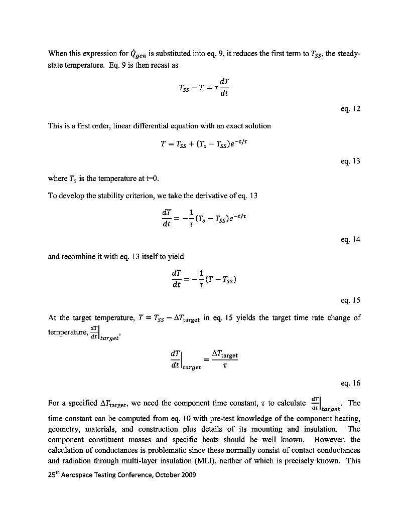
When this expression for is substituted into eq. 9, it reduces the first term to , the steady-
state temperature. Eq. 9 is then recast as
eq. 12
This is a first order, linear differential equation with an exact solution
eq. 13
where is the temperature at t=0.
To develop the stability criterion, we take the derivative of eq. 13
eq. 14
and recombine it with eq. 13 itself to yield
eq. 15
At the target temperature, in eq. 15 yields the target time rate change of
temperature, dT ,
dt target
eq. 16
For a specified , we need the component time constant, to calculate . The
time constant can be computed from eq. 10 with pre-test knowledge of the component heating,geometry, materials, and construction plus details of its mounting and insulation. Thecomponent constituent masses and specific heats should be well known. However, thecalculation of conductances is problematic since these normally consist of contact conductancesand radiation through multi-layer insulation (MLI), neither of which is precisely known. This
25th Aerospace Testing Conference, October 2009
leads to errors in the calculation of the conductances as well as errors in the pre-test prediction of. Because of these factors, the value of predicted pre-test should be relied on as only a pre-
test guide. An accurate representation of the component time constant must be calculated real-time from data obtained during the normal course of a thermal-vacuum test. This calculation isdetailed next.
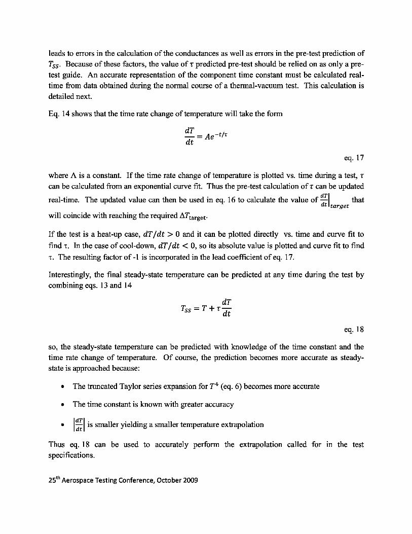
Eq. 14 shows that the time rate change of temperature will take the form
eq. 17
where A is a constant. If the time rate change of temperature is plotted vs. time during a test, ican be calculated from an exponential curve fit. Thus the pre-test calculation of can be updated
real-time. The updated value can then be used in eq. 16 to calculate the value of thatdt target
will coincide with reaching the required .
If the test is a heat-up case, and it can be plotted directly vs. time and curve fit to
find . In the case of cool-down, , so its absolute value is plotted and curve fit to find
. The resulting factor of -1 is incorporated in the lead coefficient of eq. 17.
Interestingly, the final steady-state temperature can be predicted at any time during the test bycombining eqs. 13 and 14
eq. 18
so, the steady-state temperature can be predicted with knowledge of the time constant and thetime rate change of temperature. Of course, the prediction becomes more accurate as steady-state is approached because:
• The truncated Taylor series expansion for (eq. 6) becomes more accurate
• The time constant is known with greater accuracy
• I dT I is smaller yielding a smaller temperature extrapolationdt
Thus eq. 18 can be used to accurately perform the extrapolation called for in the testspecifications.
25th Aerospace Testing Conference, October 2009

APPLICATION OF METHODOLOGY
Application of the proposed methodology is accomplished by executing the following steps:
1. Obtain the component time constant, , from pre-test analysis or by using eq. 10. This is afirst approximation of the true time constant.
2. Specify a target temperature difference, , and calculate the preliminary temperature
change value, , associated with this temperature using eq. 16.dt target
3. During the test, calculate the current component temperature time rate of change, , from
available test data. Perform an exponential curve fit of at I vs. t to refine .
4. Use the updated estimate of obtained in step 3 to refine
as a termination criterion.dt target
Repeat as needed.
5. When measured during the test becomes less than the updated value of dT
dt dt I,
acceptable temperature stabilization has been achieved.
Application of this methodology results in knowledge that the temperature is within of
the steady state temperature during test without knowing the true steady-state temperaturebeforehand.
TEST VALIDATION OF METHODOLOGY
A thermal-vacuum test was performed to validate the methodology. Two simple heatedconfigurations were tested in separate runs in a thermal vacuum chamber: 1) heat transferdominated by radiation to the chamber cold walls and 2) the dominant mode of heat transfer wasconduction to a temperature-controlled plate.
Configuration 1 ± This test article was a heated cube constructed from 3.175 mm (0.125 in)thick aluminum plate. The cube measured 153 mm (6 in) on each side. Its surface was coatedwith two layers of Kapton® tape to improve its emissivity ( = ~0.7). The cube contained sixinternal thermocouples ± one on each face. A small controlled conductive heat transfer path tothe chamber wall was provided by a 0.305 m (1 ft) long Mylar ®-covered 9.53 mm (3/8 in) outerdiameter copper support tube with a 0.89 mm (0.035 in) wall thickness. Two thermocoupleswere mounted on the support tube to monitor heat flow. The cube included two internal 39 W
$ The temperature-time results of a pretest analysis provide vs. time. An exponential curve fit is used to
calculate .25th Aerospace Testing Conference, October 2009

Kapton® film heaters mounted on opposite walls. These heaters were powered by a controlleddirect current (DC) voltage source.
Configuration 2 – This test article was similar to Configuration 1. It was made of aluminum and
had the same size, thickness, and thermocouple and heater layout. A single layer of low saluminized Mylar® ( = ~0.05) covered the box to reduce its radiation heat transfer. A single 1/4x 28 stainless steel bolt attached the cube to a 0.305 by 0.305 m (12 by 12 inch) 6.35 mm(1/4 inch) thick aluminum plate. The exposed plate was covered with Kapton ® tape to improveits emissivity. Two Variac powered 125 W bar heaters were bolted to the underside of the plate.Three thermocouples were mounted on the plate to sense its temperature – one in the center nearthe connecting bolt and two near the heaters.
The test configurations are depicted schematically in Figures 1 and 2. Photos of the actual testset-ups are presented in Figures 3 and 4. In the data discussion, the thermocouples are denotedas “top” , “bottom”, and “side”, corresponding to their relative locations in the chamber. Theplate thermocouple near the bolt in Configuration 2 is taken as the plate temperature.
Figure 1 f Test Configuration 1
25th Aerospace Testing Conference, October 2009

Figure 2 f Test Configuration 2
Figure 3 f Test Configuration 1
25th Aerospace Testing Conference, October 2009
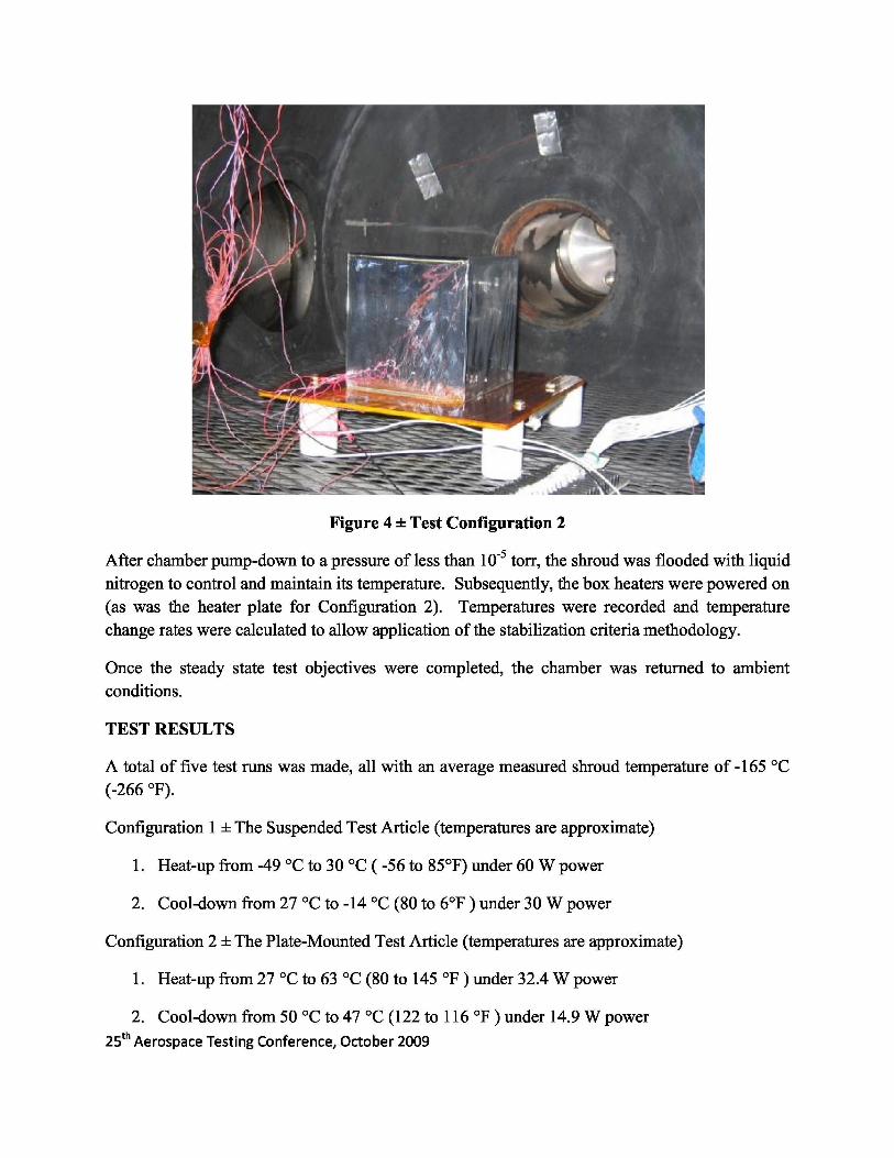
Figure 4 f Test Configuration 2
After chamber pump-down to a pressure of less than 10 -5 torr, the shroud was flooded with liquidnitrogen to control and maintain its temperature. Subsequently, the box heaters were powered on(as was the heater plate for Configuration 2). Temperatures were recorded and temperaturechange rates were calculated to allow application of the stabilization criteria methodology.
Once the steady state test objectives were completed, the chamber was returned to ambientconditions.
TEST RESULTS
A total of five test runs was made, all with an average measured shroud temperature of -165 °C(-266 °F).
Configuration 1 ± The Suspended Test Article (temperatures are approximate)
1. Heat-up from -49 °C to 30 °C ( -56 to 85°F) under 60 W power
2. Cool-down from 27 °C to -14 °C (80 to 6°F ) under 30 W power
Configuration 2 ± The Plate-Mounted Test Article (temperatures are approximate)
1. Heat-up from 27 °C to 63 °C (80 to 145 °F ) under 32.4 W power
2. Cool-down from 50 °C to 47 °C (122 to 116 °F ) under 14.9 W power25th Aerospace Testing Conference, October 2009

3. Heat-up from 43 °C to 46 °C (110 to 114 °F ) under 14.9W power
A detailed discussion of the first test run of each configuration follows. All of the test runs
behaved similarly - the time rate change of temperature, dt displayed the expected exponential
form of as the temperatures neared steady-state.
Configuration 1 - The suspended cube heat-up test temperature history is shown in Figure 5. Theinitial part of the plot is an unpowered cool-down. 60 W of heater power was applied at 0.533hours. The six measured temperatures (one on each side of the box) show the expectedasymptotic approach to the final temperature.
Figure 5 f Hanging Cube Temperatures
Figure 6 shows the difference between the maximum recorded average temperature (taken as thesteady-state average temperature) and the average measured temperature. The straight linenature of the plot after 1.5 hours shows that the exact exponential solution for temperature(eq. 13) will hold as steady-state is approached - as predicted by the theory. The increasedscatter near the end of the test is caused by the increased relative effect of thermocouplemeasurement instabilities as steady-state is approached.
25th Aerospace Testing Conference, October 2009
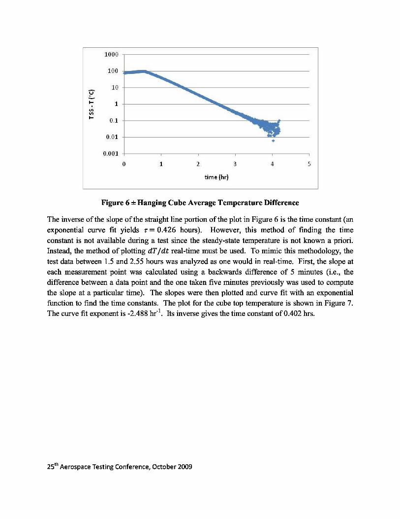
Figure 6 f Hanging Cube Average Temperature Difference
The inverse of the slope of the straight line portion of the plot in Figure 6 is the time constant (anexponential curve fit yields hours). However, this method of finding the timeconstant is not available during a test since the steady-state temperature is not known a priori.Instead, the method of plotting real-time must be used. To mimic this methodology, thetest data between 1.5 and 2.55 hours was analyzed as one would in real-time. First, the slope ateach measurement point was calculated using a backwards difference of 5 minutes (i.e., thedifference between a data point and the one taken five minutes previously was used to computethe slope at a particular time). The slopes were then plotted and curve fit with an exponentialfunction to find the time constants. The plot for the cube top temperature is shown in Figure 7.The curve fit exponent is -2.488 hr -1 . Its inverse gives the time constant of 0.402 hrs.
25th Aerospace Testing Conference, October 2009

Figure 7 f Time Rate Change of Temperature for the Top of the Hanging CubeTemperature
The time constants calculated in a similar fashion for all six thermocouple locations are listed inTable 1.
Table 1 f Time Constants for The Hanging CubeCalculated Real-Time
Location Top Side 1 Side 2 Side 3 Side 4 Bottom Average Valuei (hours) 0.402 0.373 0.410 0.401 0.405 0.402 0.399
The average time constant calculated for the cube is 0.399 hours ± within 7% of the time
constant calculated from Figure 6. The real-time calculated value of hours can beused to calculate the predicted steady-state temperature at any time during the test using eq. 18.These predicted temperatures are shown in Figure 8. The figure also shows the times where thetemperature was expected to be within 1 °C and 0.5 °C of steady-state by the theory (2.65 and2.85 hours, respectively). The agreement between theory and experiment is excellent.
25th Aerospace Testing Conference, October 2009
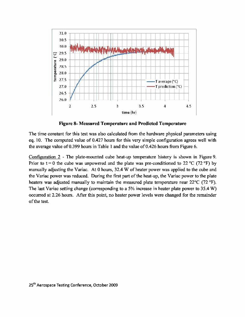
Figure 8- Measured Temperature and Predicted Temperature
The time constant for this test was also calculated from the hardware physical parameters usingeq. 10. The computed value of 0.427 hours for this very simple configuration agrees well withthe average value of 0.399 hours in Table 1 and the value of 0.426 hours from Figure 6.
Configuration 2 - The plate-mounted cube heat-up temperature history is shown in Figure 9.Prior to t = 0 the cube was unpowered and the plate was pre-conditioned to 22 °C (72 °F) bymanually adjusting the Variac. At 0 hours, 32.4 W of heater power was applied to the cube andthe Variac power was reduced. During the first part of the heat-up, the Variac power to the plateheaters was adjusted manually to maintain the measured plate temperature near 22°C (72 °F).The last Variac setting change (corresponding to a 5% increase in heater plate power to 35.4 W)occurred at 2.26 hours. After this point, no heater power levels were changed for the remainderof the test.
25th Aerospace Testing Conference, October 2009

Figure 9 f Plate-Mounted Cube Temperatures
The plate temperature measured near the cube mounting bolt () shows a slight temperature
increase during the latter portion of the test. The average increase after 2.26 hours is0.223 °C/hour (0.402 °F/hour). This temperature rise is equivalent to 0.16 W of excess heating§,which is negligible compared to both the 32.4 W of box heating and the 35.4 W of plate heating.However, this upward temperature creep must be removed from the data before stability can beassessed.
To remove the test temperature creep, we add a correction of - 0.223 t to all thetemperature data after 2.26 hours. The correction is in °C and t is the elapsed time in hours. Asample of the data with and without the correction is shown in Figure 10.
§ Based on the combined thermal mass of the test cube and the mounting plate.25th Aerospace Testing Conference, October 2009

Figure 10 f Raw and Corrected Average Cube Temperatures
The corrected temperature traces are shown in Figure 11.
Figure 11 f Corrected Plate-Mounted Cube Temperatures
To verify the methodology for this case, the corrected test data between 1.6 and 2.8 hours wasanalyzed as one would in real-time. First, the slope at each measurement point was determinedusing a backwards difference of 5 minutes. The slopes were then plotted and curve fit to find thetime constants. The results for each thermocouple are listed in Table 2.
25th Aerospace Testing Conference, October 2009

Table 2 f Time Constants for the Plate-Mounted CubeCalculated Real-Time
Location Top Side 1 Side 2 Side 3 Side 4 Bottom Average Valuez (hours) 1.036 1.076 1.015 1.053 1.040 1.076 1.049
The average time constant for the cube is 1.049 hours. As before, this time constant can be usedat any time during the test to calculate the predicted steady-state temperature using eq. 18. Thepredicted temperatures are shown in Figure 12. The figure also shows the times where thecurrent temperature was within 1 °C and 0.5 °C by the theory (3 and 3.8 hours, respectively). Asbefore, the agreement between theory and experiment is excellent.
Figure 12- Measured Temperature and Predicted Temperature
The time constant for this test was also calculated from eq. 10 using the physical configuration.Based on a bolt interface resistance of 0.7 K/W 6 and a cube emissivity of 0.05, the value of thetime constant for this test is 0.210 hours, which is in very poor agreement with the test calculatedvalue of 1.049 hours. Even for this fairly simple configuration, the complication of a poorlyknown interface conductance makes the pre-test calculated value of inaccurate. However, byassessing during the test, an accurate value of the time constant can be obtained and thestability criterion can be applied accurately.
25th Aerospace Testing Conference, October 2009

OTHER CONSIDERATIONS
For the methodology of the present work to be accurate, two conditions must be met: the unitunder test must be thermally relaxed and the required time rate change of temperature must bemeasurable and readable. These conditions are discussed below.
Internal Thermal Relaxation ± A test article will have an internal thermal relaxation timeconstant, ,
eq. 19
where L is a characteristic length of the unit and LOtheOqnit’sOtheQLW¶Vfq WKHUPDObyGLIIXVLYLW\q JL
eq. 20
where , , and are the effective thermal conductivity, density, and specific heat of
the unit, respectively.
If the internal thermal relaxation time is much shorter than the time constant for heat transfer tothe environment (eqs. 10 and 17), the unit will be thermally relaxed when the acceptable steady-state condition is reached.
Typical spacecraft components have internal thermal relaxation times on the order of one hour.Many hours are generally required for stability in thermal-vacuum testing, so the relaxationcriterion is normally met. Table 3 lists the internal thermal relaxation times for representativeactive thermal control system components for the International Space Station (ISS), all of whichare less than 1 hour.
25th Aerospace Testing Conference, October 2009

Table 3 f Typical ISS Active Thermal Control System Hardware Thermal Relaxation TimeConstants
Measurement Accuracy and Precision ± For massive components to meet reasonable stabilityrequirements, the necessary time rate change of temperature may need to be less than 1 °C/hr.Normal data acquisition system level temperature measurement accuracy for resistancetemperature detectors (RTDs) and thermocouples is no better than ±1.5 °C. Although thereading itself has a relatively large error, undisturbed RTDs and thermocouples can veryaccurately sense temperature changes. The standard accuracies quoted by the manufacturer 7 are±0.005 °C/°C for RTDs and ±0.0075 to 0.015 °C/°C for thermocouples. This yields aninstrument error of less than 1.5% when changes in temperature are measured. Data acquisitionsystems are also very stable. Because their error normally appears as an offset in the measureddata, they too can yield accurate data for small temperature changes. If the data system is set upwith sufficient granularity (i.e., bit flips at small enough intervals of temperature), it will yielddata that provides an accurate measurement of the time rate change of temperature. This isespecially true if graphical or averaging methods are used to smooth the digital data.
CONCLUDING REMARKS/RECOMMENDATION
A physics-based methodology for establishing thermal-vacuum test temperature stabilization hasbeen developed and verified. The time constant of the test article is calculated pre-test, but mustbe updated during the test. With a refined time constant and a user-specified target temperaturedifference, a target time rate change of temperature is established. Once this rate is observedduring test, the required temperature stabilization has been achieved. This methodology is apowerful, broadly applicable tool that can be used in thermal-vacuum testing to obtain acceptablesteady-state measurements while minimizing test time. It is recommended that this technique beapplied to properly couple the normally separate temperature stabilization criteria presented inthe reviewed standards and requirements.
25th Aerospace Testing Conference, October 2009
REFERENCES
1. Space Shuttle Specification, Environmental Acceptance Testing, SP-T-0023, Revision C,May 17, 2001.
2. Constellation Environmental Qualification and Acceptance Testing Requirements(CEQATR), CxP 70037 Revision B, Final, December, 17, 2008.
3. Qualification and Acceptance Environmental Test Requirements, International SpaceStation, SSP 41172, Revision Y, May 23, 2007.
4. Military Standard, Test Requirements for Launch, Upper Stage, and Space Vehicles, MIL-STD-1540C, September 15, 1994.
5. Department of Defense Test Method Standard for Experimental Engineering Considerationand Laboratory Tests, MIL-STD-810F, January 1, 2000.
6. Spacecraft Thermal Control Handbook, David G. Gilmore, Ed., 2nd Ed., The AerospacePress, 2002.
7. The Omega® Temperature Measurement Handbook and Encyclopedia, Vol. MMX, 6 th
edition, Omega Engineering, Stamford, CT.
BIOGRAPHIES
Mr. Rickman is the NASA Technical Fellow for Passive Thermal and joined the NASAEngineering and Safety Center in 2009. In this capacity, he leads technical assessments for highrisk programs and promotes stewardship of the passive thermal control and thermal protectiondisciplines. Previously, Mr. Rickman was the Chief of the Thermal Design Branch as the NASA± Lyndon B. Johnson Space Center (JSC) where he led a group of more than forty civil servantsand contractors focusing on passive thermal control and entry thermal protection, system andsubsystem management for the Space Shuttle, International Space Station and Constellationprograms, and entry thermal protection system testing. His interests include thermal analysis andpassive thermal control of orbiting spacecraft. He has authored or co-authored a dozenpublications including a chapter on natural and induced thermal environments for the textbookSafety Design for Space Systems (Elsevier, 2009). He holds a patent as a co-inventor of aninnovative single-launch space station concept. Mr. Rickman earned a BS degree in AerospaceEngineering from the University of Cincinnati and a MS degree in Physical Science from theUniversity of Houston at Clear Lake.
Dr. Ungar has degrees in mechanical engineering from the University of Cincinnati, theUniversity of Kentucky, and the University of Houston. His dissertation was on boiling heattransfer. He has worked at NASA/JSC for the last twenty years in the area of single phase and
25th Aerospace Testing Conference, October 2009

two-phase heat transfer and fluid flow. Over that time he has participated in the design,performance, and post-test analysis of numerous tests. He is a member of ASME.
25th Aerospace Testing Conference, October 2009