Embed Size (px)
Citation preview

A Platform for High-Speed Biomechanical Analysis Using Wearable Wireless Sensors
by
Michael T Lapinski
S.M., Massachusetts Institute of Technology (2008)M.S, Rensselaer Polytechnic Institute(2002)B.S., Rensselaer Polytechnic Institute(2000)
Submitted to the Program in Media Arts and Sciences,School of Architecture and Planning,
in partial fulfillment of the requirements for the degree ofDoctor of Philosophy in Media Arts and Sciences
at the
MASSACHUSETTS INSTITUTE OF TECHNOLOGY
September 2013
© Massachusetts Institute of Technology 2013. All rights reserved.
AuthorProgram in Media Arts and Sciences
August 9, 2013
Certified byJoseph A. Paradiso
Associate Professor of Media Arts and SciencesMIT Media Lab
Thesis Supervisor
Accepted byProf. Patricia Maes
Associate Academic HeadProgram in Media Arts and Sciences

2
3
A Platform for High-Speed Biomechanical Analysis Using Wearable Wireless Sensors
by
Michael T Lapinski
Submitted to the Program in Media Arts and Sciences,School of Architecture and Planning, on August 9, 2013
in partial fulfillment of the requirements for the degree ofDoctor of Philosophy in Media Arts and Sciences
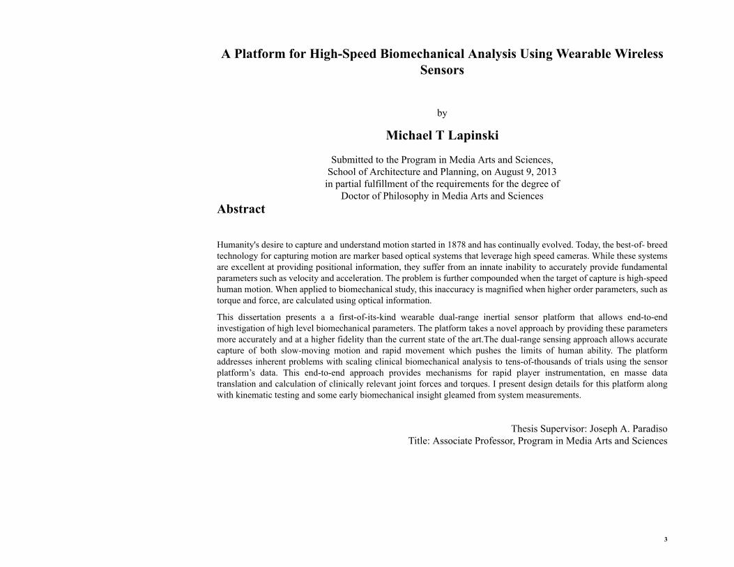
Abstract
Humanity's desire to capture and understand motion started in 1878 and has continually evolved. Today, the best-of- breed technology for capturing motion are marker based optical systems that leverage high speed cameras. While these systems are excellent at providing positional information, they suffer from an innate inability to accurately provide fundamental parameters such as velocity and acceleration. The problem is further compounded when the target of capture is high-speed human motion. When applied to biomechanical study, this inaccuracy is magnified when higher order parameters, such as torque and force, are calculated using optical information.
This dissertation presents a a first-of-its-kind wearable dual-range inertial sensor platform that allows end-to-end investigation of high level biomechanical parameters. The platform takes a novel approach by providing these parameters more accurately and at a higher fidelity than the current state of the art.The dual-range sensing approach allows accurate capture of both slow-moving motion and rapid movement which pushes the limits of human ability. The platform addresses inherent problems with scaling clinical biomechanical analysis to tens-of-thousands of trials using the sensor platform’s data. This end-to-end approach provides mechanisms for rapid player instrumentation, en masse data translation and calculation of clinically relevant joint forces and torques. I present design details for this platform along with kinematic testing and some early biomechanical insight gleamed from system measurements.
Thesis Supervisor: Joseph A. ParadisoTitle: Associate Professor, Program in Media Arts and Sciences

4

5
A Platform for High-Speed Biomechanical Analysis Using Wearable Wireless Sensors
by
Michael T Lapinski
The following people served as readers for this thesis:
Thesis ReaderThomas M. Kepple
Chief Science OfficerC-Motion, Incorporated
Thesis ReaderDr. Eric Berkson
Director, Mass General Orthopedics Sports Performance CenterAssistant in Orthopedic SurgeryMassachusetts General Hospital
InstructorHarvard School of Medicine

6

7
AcknowledgmentsAsia for all of the support and everything else that you know you did along the way.
Mom and Dad, looks like I will end up in San Francisco anyway, but not as a pro skateboarder living in a cardbord box like I promised 18 years ago...
The entire Responsive Environments group. The nerds who taught me so much and helped me unlock the macgic of those little black chips on that are found on circuit boards and helping me create my own magic, especially Mat Laibowitz. Without your guidance I probably wouldn't have finished this thing.
Brian Mayton for the analog and digital separation of powers and grounds and all the great advice along the way. Your patience with clowns like me guarantees you will be a great professor someday.
Matt Aldrich for all of the math help and guidance. Also for 4 years of putting up with the Slayer, tupperwares, speaker phone and other countless annoying things.
Nan-Wei, just for being Nan-Wei.
Matt Xmal, whose words "voltage is like water" stick with me to this day.
Mark Feldmeier, I suspect you and your pile will never disappear from the lab and it makes me smile.
Tom Kepple, the shining beacon of light who taught me more about motion capture in half a year than I figured out on my own in 5 years. Your insight, timeliness and guidance were invaluable.
Eric, for expecting more from me than I thought I was capable of, the shoulder and knee surgeries and direction along this 7 year trip.
John Geen @ Analog Devices, you know much more about MEMs than I ever will, but had no problem sharing some of that knowledge with me.
Analog Devices and Grace Pigott and John Memishiam, for all the free gyros, accelerometers and connections to the people in the know.
Steve Buckley from Corflex, the neoprene attachment system still lives and will live for a long time to come.
Sean Driscoll, its in there and up to you to find it.
Clemens, Why that?
Donna and Hollie for the time in the sport performance lab and all of the help.
Linda P, you are the bestest and that's it.
Cornelle King and Kevin Davis, you guys are waaaay under appreciated. I appreciate everything you guys do to keep the media lab going.
8
To all my sponsors that kept me racing:
- The MIT GSC
- Colleen Asch at Asterisk
- Richard Basinger at Yoshimura
- Steve-O, Zak and Ziggy at Factory Connection
- Devin Leblanc from MSR and Pro Taper
- Tim Sprague from S4MX
- Rich Taylor at EKS Brand goggles
- Ryan at Works Connection
- Dunlop Tires
- Acerbis Plastics
- Gaerne Boots
- Leatt Brace for keeping my neck in one piece
- Magura Clutches

. . .
. .
T
. . . .
. . . . . . . . . . . . . . . . . . . . . . . . . . . . . . . . . . . . . .CONTENTS
he end of the beginning or the beginning of the end?
The Contents chapter contains the spoilers, in other words the Table of Contents and List of Figures.
A Platform for High-Speed Biomechanical Analysis Using Wearable Wireless Sensors 9

. . . . . . . . . . . . . . . . . . . . . . . . . . . . . . . . . . . . . . . . . . . . . . . . . . . . . . . . . . .T A B L E O F C O N T E N T S
Contents ..................................................................9Table of Contents ..................................................................... 10
Chapter 1 - Introduction ........................................171.1.1 A Few Words on Biomechanics.................................................191.1.2 Optical System Synopsis ............................................................19
1.2 Consumers of Sensor Fruit [Motivations]........................ 201.2.1 Injury Mechanisms.....................................................................231.2.2 Motivations for Using Inertial Sensors ......................................24
1.3 Research Guidelines......................................................... 251.3.1 Hardware Guidelines..................................................................261.3.2 Data Management Guidelines ....................................................271.3.3 Data Processing Fundamentals...................................................281.3.4 Biomechanically Relevant Data Processing...............................29
Chapter 2 - Prologue .............................................312.1 Related Work ................................................................... 32
2.1.1 Motion Capture Systems ............................................................322.1.2 Marker Based Optical Trackers..................................................35
2.1.2.1 Active Systems .........................................................................................352.1.2.2 Semi-Passive Systems...............................................................................362.1.2.3 Fully Passive Systems...............................................................................37
2.1.3 Inertial Systems for Motion Capture ..........................................372.1.4 Current Pitcher Development.....................................................392.1.5 Precision of Biomechanical Research ........................................40
2.1.5.1 Tracking Marker and the Underlying Skeleton ........................................412.1.5.2 Marker Set Used .......................................................................................42
10 Michael T Lapinski

. . .
. .
2.1.5.3 Position and Orientation Calculation Methods.........................................422.1.5.4 Inertial Parameter Estimation ...................................................................43
Chapter 3 - Taxonomy, High Level Architecture & Kinetic Model .......................................................45
3.1 Taxonomy ........................................................................ 463.1.0.1 Player ........................................................................................................463.1.0.2 Session ......................................................................................................473.1.0.3 Gesture......................................................................................................493.1.0.4 Purposes of Player and Gesture Annotation .............................................50
3.2 System Architecture......................................................... 513.2.1 Field Deployment.......................................................................513.2.2 µSD Data Retrieval Interface .....................................................523.2.3 Data Import Engine ....................................................................523.2.4 Visualization, Analysis and Modeling .......................................54
3.3 Physical (Kinematic) Model ............................................ 543.3.1 Coordinate Systems....................................................................543.3.2 Landmark Definition ..................................................................553.3.3 Segment Definition ....................................................................563.3.4 Joint Definition...........................................................................583.3.5 Performing the Kinematics.........................................................59
3.4 Kinetic Model .................................................................. 59
Chapter 4 - The Tangible ......................................614.1 Wireless Inertial Measurement Node............................... 62
4.1.1 Main Board.................................................................................634.1.2 Inertial High Range Daughterboards..........................................654.1.3 Wireless Expansion Board .........................................................654.1.4 Putting It All Together ...............................................................664.1.5 System Evolution .......................................................................68
4.2 Calibration........................................................................ 69
A Platform for High-Speed Biomechanical Analysis Using Wearable Wireless Sensors 11

4.2.1 Rotation Based Calibration ........................................................704.2.1.1 Gyroscopes................................................................................................704.2.1.2 Accelerometers .........................................................................................71
4.2.2 Calibration Rig ...........................................................................754.2.2.1 Motor and Controller ................................................................................774.2.2.2 Motor Containment...................................................................................784.2.2.3 Per Axis Node Motor Attachment ............................................................79
4.2.3 Calibration Process.....................................................................804.2.4 Calibration Results .....................................................................81
4.3 Network Control Basestation ........................................... 834.3.1 Optical System Synchronization ................................................84
4.4 Data Translator................................................................. 85
Chapter 5 - The Intangible ....................................875.1 Basestation ....................................................................... 88
5.1.1 Optical System Synchronization ................................................935.2 Node Startup..................................................................... 95
5.2.1 Flash Memory ............................................................................975.2.2 Error Handling Subsystem .........................................................975.2.3 Clocks and Peripheral Bus .........................................................985.2.4 Communication Peripherals .......................................................985.2.5 Hardware Devices ....................................................................100
5.2.5.1 µSD Card ................................................................................................1005.2.5.2 High Range Gyroscopes .........................................................................1005.2.5.3 High Range Accelerometer.....................................................................1005.2.5.4 Analog-to-Digital Converter...................................................................1015.2.5.5 Low Range Gyroscope............................................................................1025.2.5.6 Low Range Accelerometer .....................................................................1025.2.5.7 Magnetometer .........................................................................................1035.2.5.8 RF Transceiver........................................................................................103
5.3 Node Operation .............................................................. 1045.3.0.1 Error Commands.....................................................................................1045.3.0.2 Idle Command.........................................................................................1055.3.0.3 Next Packet Command ...........................................................................105
12 Michael T Lapinski
. . .
. .
5.3.0.4 Erase Flash Command ............................................................................1055.3.0.5 Sample to Flash Command.....................................................................1055.3.0.6 Pseudo-Command Continuous Mode .....................................................1075.3.0.7 Sample Count Command........................................................................1085.3.0.8 Get Filename Command .........................................................................108
5.4 Data Translator............................................................... 109
Chapter 6 - Tangible Intangibles ........................1116.1 Network Control Application......................................... 112
6.1.1 USB Connection.......................................................................1146.1.2 Network Configuration ............................................................1146.1.3 Erasing Flash ............................................................................1156.1.4 Sampling Gesture Data.............................................................1156.1.5 Continuous Sampling ...............................................................1166.1.6 Error Management....................................................................1166.1.7 Reading Node Contents............................................................1176.1.8 Optical System Synchronization ..............................................117
6.2 Data Translation Application ......................................... 1176.2.1 USB Connection.......................................................................1196.2.2 Translating Data .......................................................................120
6.3 Data Model..................................................................... 1236.3.1 Player Data Model....................................................................1256.3.2 Session Data Model..................................................................1276.3.3 Gesture Data Model .................................................................1276.3.4 Node Data Model .....................................................................1306.3.5 Visual3D Data Model...............................................................132
6.4 Data Processing and Import Application - Operator View..134
6.4.1 Database Connectivity..............................................................1346.4.2 Player Management..................................................................1366.4.3 Session Management................................................................1386.4.4 Gesture Handling......................................................................138
A Platform for High-Speed Biomechanical Analysis Using Wearable Wireless Sensors 13

6.4.4.1 Gesture Import Process ...........................................................................1396.4.4.2 Gesture Annotation and Management ....................................................141
6.4.5 Miscellaneous Operator Features .............................................1436.5 . Data Processing and Import Application - User View. 145
Chapter 7 - Experimental Methods .....................1477.1 Body Attachment ........................................................... 148
7.1.1 2009..........................................................................................1487.1.2 2010..........................................................................................153
7.2 Pitching Protocol ............................................................ 1607.3 Batting Protocol ............................................................. 163
7.3.1 Directed Batting Protocol.........................................................1637.3.2 Batting Practice Protocol..........................................................168
7.4 Dual System Experiments .............................................. 1697.5 Data Translation and Annotation ................................... 170
7.5.1 Pitch Annotation.......................................................................1727.5.2 Swing Annotation.....................................................................1737.5.3 Dual System Annotation ..........................................................174
Chapter 8 - Validation and Error Sources ...........1758.1 Error Quantification ....................................................... 176
8.1.1 Calibration................................................................................1768.1.2 Application (Coordinate System Misalignment)......................1798.1.3 Soft Tissue Artifacts.................................................................1808.1.4 Acceleration Induced Gyroscope Error....................................184
8.2 System Validation .......................................................... 1868.2.1 The Inertial Gold Standard.......................................................1888.2.2 The Eyeball Comparison..........................................................1928.2.3 Angular Velocity Comparison .................................................1968.2.4 Angular Acceleration and Deceleration ...................................200
14 Michael T Lapinski

. . .
. .
Chapter 9 - Analytics and Biomechanical Metrics ...203
9.1 Data Processing Fundamentals ...................................... 2049.2 Data Viewing ................................................................. 2069.3 Segment Gesture Statistics............................................. 210
9.3.1 Gesture Duration Determination ..............................................2109.3.2 Individual Segment Analysis ...................................................2119.3.3 Inter-Segment Timing ..............................................................2129.3.4 Segment Velocity Estimation...................................................212
9.4 Session Aggregation and Statistics ................................ 2159.4.1 Session Stat Sheet ....................................................................2159.4.2 Segment Timing Analysis Application ....................................218
9.5 Like Modality Sensor Fusion......................................... 2219.6 Biomechanical Metrics .................................................. 225
9.6.1 Jerk ...........................................................................................2269.6.2 Shoulder Distraction Jerk .........................................................2319.6.3 Shoulder Internal and External Rotation Acceleration ............232
9.7 Calculation of Kinetics and Dynamics........................... 2379.7.1 Visual3D Integration ................................................................2379.7.2 Example Data ...........................................................................2409.7.3 Shoulder Distraction and Compression Forces ........................2469.7.4 Elbow Valgus and Varus Torque .............................................2499.7.5 The Fine Print...........................................................................253
Chapter 10 - Contributions & Conclusions .........25510.1 Contributions................................................................ 25610.2 Future Work ................................................................. 258
10.2.1 Differentiation Between Real Motion & Soft Tissue Artifacts....258
A Platform for High-Speed Biomechanical Analysis Using Wearable Wireless Sensors 15

10.2.2 Coordinate System Alignment Protocols ...............................25810.2.3 Joint Angles............................................................................25910.2.4 Lower Cost Hybrid Systems ..................................................26010.2.5 Continued Data Acquisition ...................................................261
References ...........................................................263
16 Michael T Lapinski
. . .
. .I N T R O D U C T I O N
. . . .
. . . . . . . . . . . . . . . . . . . . . . . . . . . . . . . . . . . . . .INTRODUCTION
I t’s not going to write itself.
- Michael Lapinski
Here we set the stage and lead the reader into what the entire body of work will be about.
A Platform for High-Speed Biomechanical Analysis Using Wearable Wireless Sensors 17
I N T R O D U C T I O N
. . . . . . . . . . . . . . . . . . . . . . . . . . . . . . . . . . . . . . . . . . . . . . . . . . . . . . . . . . .1 . 1 A S E A S O N F O R S E N S I N G
Whether you know it or not, you don’t have to look further than your pocket to find a device that is capable of tracking you and providing a complete description of everything you have done today, how fast you have done it and can nearly predict what you will do tomorrow.
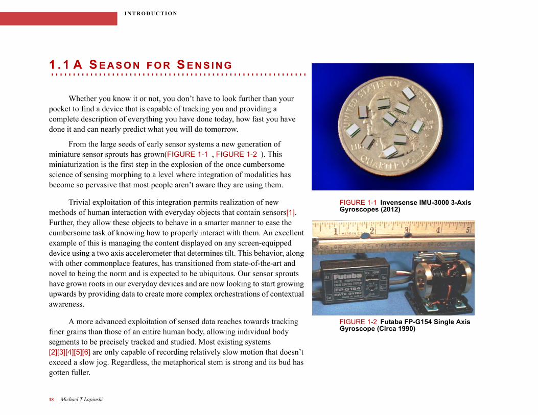
From the large seeds of early sensor systems a new generation of miniature sensor sprouts has grown(FIGURE 1-1 , FIGURE 1-2 ). This miniaturization is the first step in the explosion of the once cumbersome science of sensing morphing to a level where integration of modalities has become so pervasive that most people aren’t aware they are using them.
FIGURE 1-1 Invensense IMU-3000 3-Axis Gyroscopes (2012)
Trivial exploitation of this integration permits realization of new methods of human interaction with everyday objects that contain sensors[1]. Further, they allow these objects to behave in a smarter manner to ease the cumbersome task of knowing how to properly interact with them. An excellent example of this is managing the content displayed on any screen-equipped device using a two axis accelerometer that determines tilt. This behavior, along with other commonplace features, has transitioned from state-of-the-art and novel to being the norm and is expected to be ubiquitous. Our sensor sprouts have grown roots in our everyday devices and are now looking to start growing upwards by providing data to create more complex orchestrations of contextual awareness.
FIGURE 1-2 Futaba FP-G154 Single Axis Gyroscope (Circa 1990)
A more advanced exploitation of sensed data reaches towards tracking finer grains than those of an entire human body, allowing individual body segments to be precisely tracked and studied. Most existing systems [2][3][4][5][6] are only capable of recording relatively slow motion that doesn’t exceed a slow jog. Regardless, the metaphorical stem is strong and its bud has gotten fuller.
18 Michael T Lapinski
. . .
. .I N T R O D U C T I O N
We have reached the point or where this bud wants to blossom into a fully featured sensor “fruit” that is capable of tracking the most extreme motions that a human can perform.
1 .1 .1 A Few Words on Biomechanics
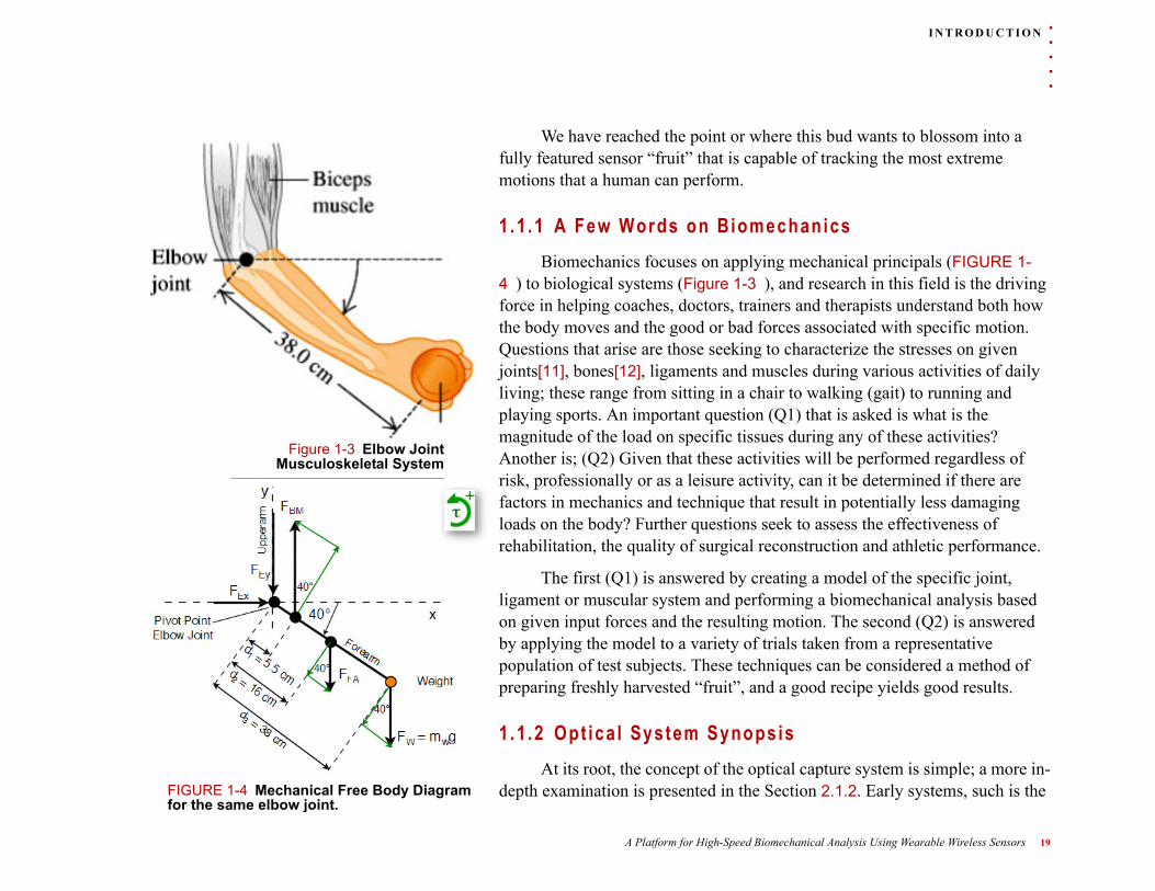
Biomechanics focuses on applying mechanical principals (FIGURE 1-4 ) to biological systems (Figure 1-3 ), and research in this field is the driving force in helping coaches, doctors, trainers and therapists understand both how the body moves and the good or bad forces associated with specific motion. Questions that arise are those seeking to characterize the stresses on given joints[11], bones[12], ligaments and muscles during various activities of daily living; these range from sitting in a chair to walking (gait) to running and playing sports. An important question (Q1) that is asked is what is the magnitude of the load on specific tissues during any of these activities? Another is; (Q2) Given that these activities will be performed
Figure 1-3 Elbow Joint Musculoskeletal System regardless of
risk, professionally or as a leisure activity, can it be determined if there are factors in mechanics and technique that result in potentially less damaging loads on the body? Further questions seek to assess the effectiveness of rehabilitation, the quality of surgical reconstruction and athletic performance.
The first (Q1) is answered by creating a model of the specific joint, ligament or muscular system and performing a biomechanical analysis based on given input forces and the resulting motion. The second (Q2) is answered by applying the model to a variety of trials taken from a representative population of test subjects.
FIGURE 1-4 Mechanical Free Body Diagram for the same elbow joint.
These techniques can be considered a method of preparing freshly harvested “fruit”, and a good recipe yields good results.
1 .1 .2 Opt ica l System Synopsis
At its root, the concept of the optical capture system is simple; a more in-depth examination is presented in the Section 2.1.2. Early systems, such is the
A Platform for High-Speed Biomechanical Analysis Using Wearable Wireless Sensors 19
I N T R O D U C T I O N
Consumers of Sensor Fruit [Motivations]
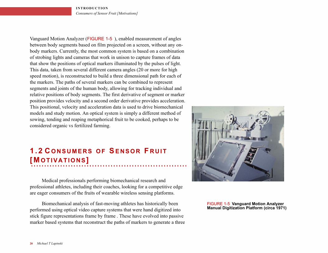
Vanguard Motion Analyzer (FIGURE 1-5 ), enabled measurement of angles between body segments based on film projected on a screen, without any on-body markers. Currently, the most common system is based on a combination of strobing lights and cameras that work in unison to capture frames of data that show the positions of optical markers illuminated by the pulses of light. This data, taken from several different camera angles (20 or more for high speed motion), is reconstructed to build a three dimensional path for each of the markers. The paths of several markers can be combined to represent segments and joints of the human body, allowing for tracking individual and relative positions of body segments. The first derivative of segment or marker position provides velocity and a second order derivative provides acceleration. This positional, velocity and acceleration data is used to drive biomechanical models and study motion. An optical system is simply a different method of sowing, tending and reaping metaphorical fruit to be cooked, perhaps to be considered organic vs fertilized farming.
1 . 2 C O N S U M E R S O F S E N S O R F R U I T
. . . . . . . . . . . . . . . . . . . . . . . . . . . . . . . . . . . . . . . . . . . . . . . . . . . . . . . . . . .[ M O T I V A T I O N S]
Medical professionals performing biomechanical research and professional athletes, including their coaches, looking for a competitive edge are eager consumers of the fruits of wearable wireless sensing platforms.
FIGURE 1-5 Vanguard Motion Analyzer Manual Digitization Platform (circa 1971)
Biomechanical analysis of fast-moving athletes has historically been performed using optical video capture systems that were hand digitized into stick figure representations frame by frame . These have evolved into passive marker based systems that reconstruct the paths of markers to generate a three
20 Michael T Lapinski
. . .
. .I N T R O D U C T I O N
Consumers of Sensor Fruit [Motivations]
dimensional representation of the motion that occurred [8][9][10]. While these systems are excellent at creating 3D images, they are lacking in the ability to accurately provide accelerations and angular velocities; Section 2.1.5 discusses this in detail. These are the starting points of any serious biomechanical analysis that wishes to assess the dynamics and calculate the forces and torques experienced by the body during high speed activity.
Meeting the need of directly obtaining the fundamental parameters to build the better biomechanical model independent of a lab-situated optical tracker is one of two primary motivations of this dissertation.
This concept is not new and was partially addressed by this author’s Master’s Thesis [7] which had a similar philosophy but did not fully realize an end-to-end system:
“A better understanding of the forces, torques and speeds enables the creation of precise biomechanical model of, for example, the shoulder and elbow. Using these models to understand the difference between proper and improper motion would give athletes the opportunity to avoid getting injured and coaches the ability to train athletes with techniques that avoid injury. Further, if there is a patient history of such motion in existence, it would be possible for physical and occupational therapists to better help athletes by refining rehabilitation protocols that accurately define the forces and torques on a body segment over time.
Even further, a system such as this can recognize that an athlete is beginning to fatigue and is in danger of injuring themselves. If this can be recognized, then the athlete can be advised as to what motion is 'safer' or be advised to stop the activity, thus avoiding injury. Another step further, if athletes can be characterized and compared in a scientific manner, it is then possible to recognize traits which lead to better performance, hence such data could act as an aid in selecting up and coming athletes.”
A Platform for High-Speed Biomechanical Analysis Using Wearable Wireless Sensors 21
I N T R O D U C T I O N
Consumers of Sensor Fruit [Motivations]
Further discussion of motivations to use inertial sensors appears in Section1.2.2. After realization of such a tool, there is a final motivation, to determine if the tool fits the job. There are two avenues that must be followed. The first is to compare the outputs of the sensor-based system to the current “gold standard”, an optical tracker. By comparing the two, optical and sensor, it will be possible to quantify the strengths and weaknesses of each. The second is to apply the system to athletes and use its data to generate meaningful and useful results that can be used in rea- world clinical research.
Complete implementation, validation and proof of concept application of such a system is the first step in changing the way that clinical research is performed by taking it from the laboratory to the athletes’ native environment, the playing field. It should be considered as a tool available to researchers, not an answer to a single research question.
Further, it is also the first step in allowing coaches and trainers to change the archaic paradigm of how athletes are developed. While there exist documented techniques for developing overhead throwing athletes[13][14], coaching is traditionally very similar to the art of ancient storytelling. Knowledge of the correct techniques and what is thought to be the proper motion has been passed down from coach to player and player to coach by word of mouth generation after generation. Again, a system such as this would be the tool that would be used to prove or disprove specific training and coaching myths in a quantitative manner without a singular answer.
Lastly, this dissertation and its models focus on baseball players and examining the motion of the upper body because they truly push the limits of what the human body can do.In principal, such a system could be applied to any sport or any athlete anywhere in the world; the only thing that is necessary is the appropriate biomechanical model to interpret and analyze the data.
22 Michael T Lapinski
. . .
. .I N T R O D U C T I O N
Consumers of Sensor Fruit [Motivations]
1 .2 .1 In jury Mechanisms
Most injury can be divided into two categories: acute injury and repetitive microtrauma. A torn Anterior Cruciate Ligament (ACL) from falling off of a ladder falls into the first and a torn ulnar collateral ligament from baseball pitching into the second. It is possible to study acute trauma, however this research focuses on repetitive microtrauma because of the science behind it, the questions it leads to, together with its huge relevance to sports. Repetitive microtrauma is defined as submaximal loading of the soft tissues. It often leads to cumulative microtrauma and eventual tissue failure. A good analogy in understanding repetitive microtrauma is to consider a rope. If you consistently yank the rope close to the point of it ripping, it will fatigue and eventually fail. This yanking is analogous to submaximal loading of the soft tissue. If tissue is constantly submaximally loaded, it will eventually fail. A specific milestone of this dissertation’s research is to gather more accurate data that is representative of this loading, thus allowing researchers to better understand the damage occurring using techniques discussed above. This allows for measurement of ongoing injury and allows prediction of future injury.
This research focuses on the overhead throwing athlete, specifically professional baseball pitchers, and the swinging athlete, professional baseball batters. The primary reason for targeting these athletes is that their motion pushes the limits of what the human body can do; throwing a baseball at 100MPH or hitting a baseball 410 feet over the green monster (a huge wall at the furthest point of the outfield in Boston’s Fenway Park) puts extreme forces on an athlete’s body and musculoskeletal system. Relatively easy access to professional players via an existing research collaboration with Massachusetts General Hospital (MGH) and a major league baseball team also plays a factor in focusing on these target subjects.
A Platform for High-Speed Biomechanical Analysis Using Wearable Wireless Sensors 23
I N T R O D U C T I O N
Consumers of Sensor Fruit [Motivations]
A factor in allowing these athletes to perform at such a high level repeatedly and consistently is the mechanics, or technique, that they have developed over time. Given a large dataset over several players, it is important to determine what it is in the mechanics of an elite player that differentiates them from others.
1 .2 .2 Mot iva t ions for Us ing Iner t ia l Sensors
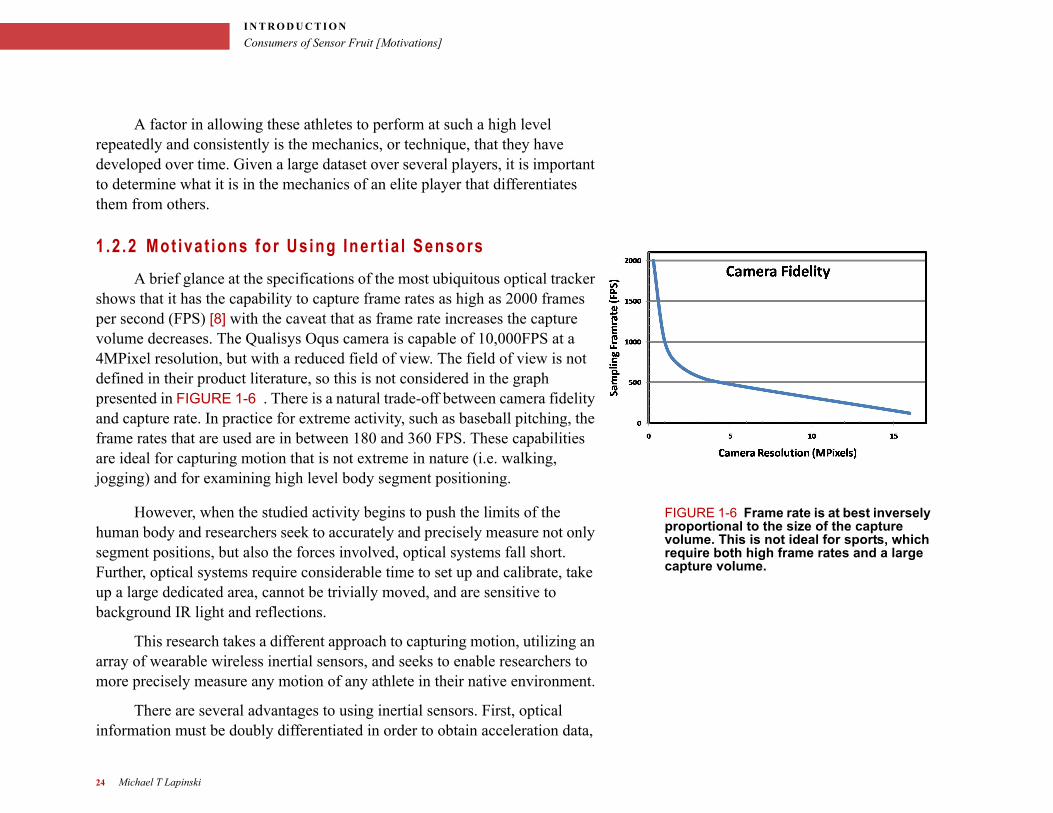
A brief glance at the specifications of the most ubiquitous optical tracker shows that it has the capability to capture frame rates as high as 2000 frames per second (FPS) [8] with the caveat that as frame rate increases the capture volume decreases. The Qualisys Oqus camera is capable of 10,000FPS at a 4MPixel resolution, but with a reduced field of view. The field of view is not defined in their product literature, so this is not considered in the graph presented in FIGURE 1-6 . There is a natural trade-off between camera fidelity and capture rate. In practice for extreme activity, such as baseball pitching, the frame rates that are used are in between 180 and 360 FPS. These capabilities are ideal for capturing motion that is not extreme in nature (i.e. walking, jogging) and for examining high level body segment positioning.
FIGURE 1-6 Frame rate is at best inversely proportional to the size of the capture volume. This is not ideal for sports, which require both high frame rates and a large capture volume.
However, when the studied activity begins to push the limits of the human body and researchers seek to accurately and precisely measure not only segment positions, but also the forces involved, optical systems fall short. Further, optical systems require considerable time to set up and calibrate, take up a large dedicated area, cannot be trivially moved, and are sensitive to background IR light and reflections.
This research takes a different approach to capturing motion, utilizing an array of wearable wireless inertial sensors, and seeks to enable researchers to more precisely measure any motion of any athlete in their native environment.
There are several advantages to using inertial sensors. First, optical information must be doubly differentiated in order to obtain acceleration data,
24 Michael T Lapinski
. . .
. .I N T R O D U C T I O N
Research Guidelines
hence any high frequency noise present in the data stream will be heavily magnified. In the case of inertial sensors, they are actually measuring the accelerations and angular velocities that are occurring (which are proportional to the induced forces) and each sensor is precisely calibrated. There is no differentiation necessary to obtain the desired measurements. The second major advantage is that a wearable system is extremely portable and can be applied wherever activity is occurring, in contrast to optical systems which require that the activity be brought into a controlled lab environment. Lastly, the maximum effective sampling rate for analog inertial sensors is strictly limited by the speed at which their output can be stored along with their intrinsic analog bandwidth. The latest generation of my inertial system is capable of sampling rates of 2 kilohertz or more, which ensures that fast changes in the studied motion will not be missed.
The study of human motion is nothing new and the de facto technology used to do this is well equipped to enable examination of most physical activity. When the activity begins to push the limits of human capability, the available systems fall short. This work seeks to apply wearable wireless inertial sensing technology, paired with massive data storage and high sampling rates, as a replacement or complementary tool to enable medical professionals to more accurately and precisely conduct research.
. . . . . . . . . . . . . . . . . . . . . . . . . . . . . . . . . . . . . . . . . . . . . . . . . . . . . . . . . . .1 . 3 R E S E A R C H G U I D E L I N E S
In order to build something it is always necessary to have some high-level goals and vision for how the system should behave and what it should consist of. These research guidelines drive what the system is and more importantly what the system is not.
A Platform for High-Speed Biomechanical Analysis Using Wearable Wireless Sensors 25
I N T R O D U C T I O N
Research Guidelines
1 .3 .1 Hardware Guide l ines
The logical place to start is the hardware that generates the data. Its criteria are:
1 Mobile - The system should be capable of being applied and recording
data anywhere that athletes train and play. The system should
seamlessly integrate with the athlete’s daily activities, rather than the
athlete fit their activities to the system.
2 Wearable - The sensing nodes should be easily and quickly attached to
the body. Fairly obvious, yet crucially important. Comfort and
placement point stability against inertial forces are all important when
attaching nodes.
3 Wireless - There should be no wires to link the nodes. Wires are
undesireable because they impede motion and make the system
more of a suit than a set of small wearable devices.
4 Rich with Sensing Modalities - Both high range and low range
gyroscopes and accelerometers should be present on all three axes
of sensing to measure inertial parameters. Additionally, a three-axis
magnetometer is needed in order to calculate orientation of each
node.
5 Synchronized - Data streams for each sensing axis intra-node should
be synchronized. Data streams between each worn node should also
be synchronized. Additionally, the system should be capable of
synchronizing with other systems, such as optical ones with a
minimum accuracy of within ±5ms to adequately compare features
from both data streams.
6 Large Data Storage - As a single node may be used on several players
for tens of minutes each, there should be enough space to store at
least this amount of data.
26 Michael T Lapinski
. . .
. .I N T R O D U C T I O N
Research Guidelines
7 Fast Sampling - In order to capture all the information possible, fast
sampling, 1 kilohertz or more, is necessary. From previous
experience, well defined peaks can be observed at this rate.
8 Precision - The data from each sensed axis should be translated from
unitless analog signals to real world inertial and magnetic heading
parameters. This requires a rigorous calibration.
9 Command and Control - A network is nothing if you cannot control its
behavior. There should be a mechanism for issuing commands that
govern the behavior of nodes attached to the body.
1 .3 .2 Data Management Guide l ines
With a set of hardware that can fulfill these functions, the amount of data that is generated grows very quickly. For example, a 5 node network sampling on 3 axes at 1 kilohertz yields about 15,000 variable-size (12-16 bit) data points per second. 1
1The system described above needs to sample 12 discrete axes.
Further, each group of nodes will record several hundred 5 second to 8 second sets of data. Simple probability leads to the conclusion that a once the hardware problem is addressed a new problem emerges, stressing the data management protocol. Fundamental needs that must be met to manage this large amount of data are:
1 Security is Paramount - Per IRB and the MIT Committee on Use of
Humans as Experimental Subjects. All data must be stored in a
secure manner with authorization and authentication in order to
access it. Further, as this technology is applied to health and injury
questions, biomechanics data becomes a measure of one's health
and may be subject to HIPPA requirements as well.
2 Identifiable - Each sensed axis must be identifiable and be linked to the
node and identifiable as coming from that node. Each group of nodes
must be linked to the athlete that was wearing them when data was
A Platform for High-Speed Biomechanical Analysis Using Wearable Wireless Sensors 27
I N T R O D U C T I O N
Research Guidelines
recorded. Individual motions must also be discretely defined to allow
for creation of metadata for each motion.
3 Metadata - Necessary metadata must also be stored and linked to a
given data stream from a node and group of nodes. This includes
anthropometric data, measurements of where nodes were placed,
information regarding classification of different motions
4 Selectable - based on the identifiable traits, there must be a
mechanism to query and select individual data streams en masse or
individually.
2It is important to note that the mentioned requirements take into account only the raw analog sensor data that makes up the bulk of what needs to be organized and stored. The amount of data that is to be managed more than doubles when the it is converted from the analog values to real calibrated angular velocities, acceleration and magnetic field readings.
5 Calibratable2 - all calibrated data must be adhere to the above 4
requirements.
Needs 1 through 4 are readily addressed by creating a data schema and storing all of the data in a relational database. Adhering to Need 5 requires a calibration process and is discussed in 4.2.
1 .3 .3 Data Process ing Fundamenta ls
With a structured data set that fulfills the necessary data management guidelines, it is natural to create methods of viewing and manipulating the data. Once the data has been processed, it is necessary to store the results of any compute-heavy processing to avoid the need to repeat them. The database mentioned in the previous section is an ideal hub for meeting these needs. There are three abilities and one ality that need to be fulfilled by this part of the system.
1 Viewability - The ability to view data for individual sensor streams.
Desirable as a simple sanity check to examine each axis of sensed
data on each node. Realtime viewability is also highly desirable.
2 Aggregatability - The ability to merge different inertial data streams is a
simple yet powerful tool for examining data and drawing conclusions.
28 Michael T Lapinski
. . .
. .I N T R O D U C T I O N
Research Guidelines
3 Repeatability - There should exist a standard set of reusable data
access components for viewing and aggregating to avoid forcing
each analyst of data to create their own.
4 Neutrality - These reusable components should be language and
location neutral. A minimum supported subset of programming
languages is MATLAB, C/C++ and Visual Basic. Each should be
capable of accessing the data in a location-neutral manner over the
network.
These four are the building blocks that allow consumers of our budding sensor fruit access to perform their own research or professional activities.
1 .3 .4 B iomechanica l ly Re levant Data Process ing
The previous sections have laid out a very application generic vision and design requirements in order to guide the development of a wearable wireless sensor network. This section outlines concepts relevant to performing a concrete biomechanical analysis, which is an eventual desired output for the specific audience of the Medical Researchers and Coaches mentioned in the introduction.
The inertial measurement unit (IMU) described in 1.3.1 is an excellent platform for tracking orientation and acceleration over time. The drawback of the IMU is that it is not aware of the context of this orientation and velocity, it does not have any idea of where it started or what it is attached to. For example, how do you compute a torque if you don’t know the radius? In order to make the IMU, or groups of IMUS, contextually aware of itself and permit tracking of it in a three dimensional space there are two requirements:
1 Mechanical Model - Information regarding the fixed locations of IMU’s
in relation to each other. Including joint locations, joint types and the
IMU’s distance form these.
A Platform for High-Speed Biomechanical Analysis Using Wearable Wireless Sensors 29

I N T R O D U C T I O N
Research Guidelines
2 Starting Point or Initial Position- A mechanism for obtaining an absolute
orientation of each IMU. This allows for tracking each node from a
known configuration.
With an initial position, it is possible to drive the mechanical model using the inertial data. In addition to yielding three dimensional positions of segments, this provides one of the key elements of a non-trivial biomechanical analysis: joint angles of body segments over time. A detailed overview of the mechanical model is presented in Section 3.3
Tackling the kinematics of the body segments leads to the real “pot of gold” for biomechanical studies, kinetic analysis. In order to calculate the kinetics of a given model, there are three requirements:
1 Joint Angles - The relation of body segments to each other
2 Center(s) of Mass - Of a single body segment or groups of them.
3 Forces - Segment masses paired with accelerations and angular
velocities acting on the segment, or group of segments.
Putting these three pieces together allows for calculation of dynamics that are the common language for describing the severity of loads experienced by joints, ligaments and tendons. A preliminary introduction as to how kinetics are calculated is presented in Section 3.4 and a more detailed discussion is presented in Section 9.7.
30 Michael T Lapinski
. . .
. .P R O L O G U E
. . . .
. . . . . . . . . . . . . . . . . . . . . . . . . . . . . . . . . . . . . .PROLOGUE
-
The Prologue chapter contains the related work to frame this research in the larger field. It is not meant to be a criticism of existing work and technology, but seeks to help readers understand how the author’s work is novel and not “reinventing the wheel”.
A Platform for High-Speed Biomechanical Analysis Using Wearable Wireless Sensors 31
P R O L O G U E
Related Work
. . . . . . . . . . . . . . . . . . . . . . . . . . . . . . . . . . . . . . . . . . . . . . . . . . . . . . . . . . .2 . 1 R E L A T E D W O R K
Other than preliminary work done in the authors Master Thesis[7], the research guidelines presented in Section 1.3 have no precedent due to the difficulty in orchestrating a standalone end-to-end wearable sensor system capable of providing complex biomechanical analysis. This does not mean that there does not exist a body of work peripheral to this dissertation from which the new technology draws.
2 .1 .1 Mot ion Capture Systems
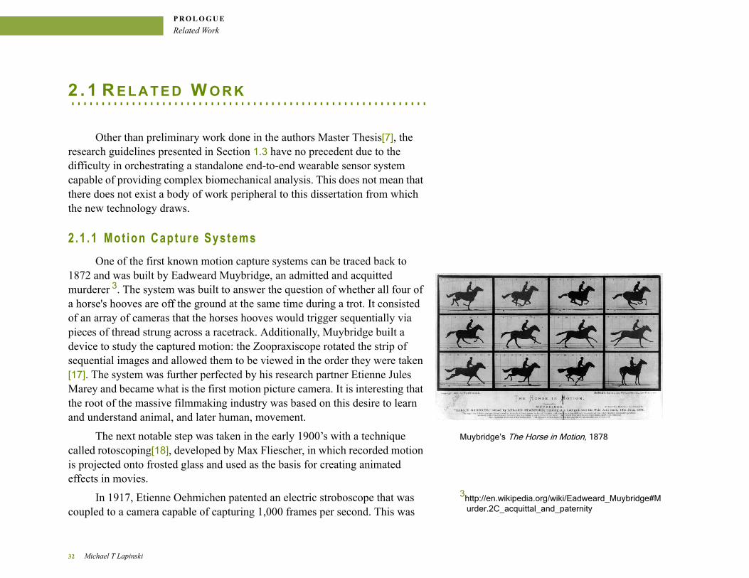
One of the first known motion capture systems can be traced back to 1872 and was built by Eadweard Muybridge, an admitted and acquitted murderer 3. The system was built to answer the question of whether all four of a horse's hooves are off the ground at the same time during a trot. It consisted of an array of cameras that the horses hooves would trigger sequentially via pieces of thread strung across a racetrack. Additionally, Muybridge built a device to study the captured motion: the Zoopraxiscope rotated the strip of sequential images and allowed them to be viewed in the order they were taken [17]. The system was further perfected by his research partner Etienne Jules Marey and became what is the first motion picture camera. It is interesting that the root of the massive filmmaking industry was based on this desire to learn and understand animal, and later human, movement.
Muybridge’s The Horse in Motion, 1878The next notable step was taken in the early 1900’s with a technique called rotoscoping[18], developed by Max Fliescher, in which recorded motion is projected onto frosted glass and used as the basis for creating animated effects in movies.
3http://en.wikipedia.org/wiki/Eadweard_Muybridge#Murder.2C_acquittal_and_paternity
In 1917, Etienne Oehmichen patented an electric stroboscope that was coupled to a camera capable of capturing 1,000 frames per second. This was
32 Michael T Lapinski
. . .
. .P R O L O G U E
Related Work
taken one step further by Harold ‘Doc’ Edgerton in 1931 when he introduced the electronic stroboscope and used it to study the motion of high speed motors in motion. This work culminated and was documented in his Sc.D dissertation that he received from MIT [19]. He did not limit his interests to mechanical systems and is also known for mid 1930’s photographs ranging from golfers swinging to animals in flight.
Not much occurred in the field until 1953, where Zeller used interrupted light markers in order to trace the motion of an athlete in a long stereo exposure [20]. This is the first mention that could be found of a ‘Witness Point’, or marker-based system.
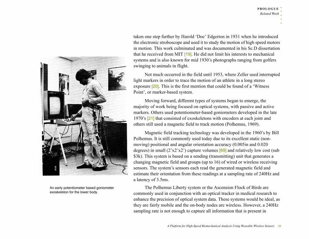
Moving forward, different types of systems began to emerge, the majority of work being focused on optical systems, with passive and active markers. Others used potentiometer-based goniometers developed in the late 1970’s [21] that consisted of exoskeletons with encoders at each joint and others still used a magnetic field to track motion (Polhemus, 1969).
Magnetic field tracking technology was developed in the 1960’s by Bill Polhemus. It is still commonly used today due to its excellent static (non-moving) positional and angular orientation accuracy (0.005in and 0.020 degrees) in small (2’x2’x2’) capture volumes [69] and relatively low cost (sub $3k). This system is based on a sending (transmitting) unit that generates a changing magnetic field and groups (up to 16) of wired or wireless receiving sensors. The system’s sensors each read the generated magnetic field and estimate their orientation from these readings at a sampling rate of 240Hz and a latency of 3.5ms.
An early potentiometer based goniometer exoskeleton for the lower body.
The Polhemus Liberty system or the Ascension Flock of Birds are commonly used in conjunction with an optical tracker in medical research to enhance the precision of optical system data. These systems would be ideal, as they are fairly mobile and the on-body nodes are wireless. However, a 240Hz sampling rate is not enough to capture all information that is present in
A Platform for High-Speed Biomechanical Analysis Using Wearable Wireless Sensors 33
P R O L O G U E
Related Work
extremely high speed motion. A second drawback is that positional data must be doubly differentiated4 in order to obtain inertial parameters, such as acceleration. They also suffer calibration issues near ferrous metal and and may require specialized rooms in which to perform data collection. These systems currently require direct AC power.
4It is important to note that double differentiation of position, which greatly magnifies any noise present in positional data, is a drawback of any system that gathers data purely based on the position of markers or wearable magnetic nodes. This includes active, passive, semi-passive and markerless optical systems.
A wearable goniometer is a device to measure joint angles. The work of Calvert et al [22] fused electronic goniometer data with hand annotated camera information and developed a language, Labnotation, in an effort to describe motion and drive stick figure animations. The electronic goniometer, a simple device by today’s standards, is a potentiometer mounted at the rotating joint of a standard goniometer. As the goniometer’s angle changes, the resistance of the potentiometer also changes, which is reflected in the output voltage of the potentiometer and can be mapped to an angle. Goniometers prove to be too bulky and restrictive for the complex motion of throwing or batting.
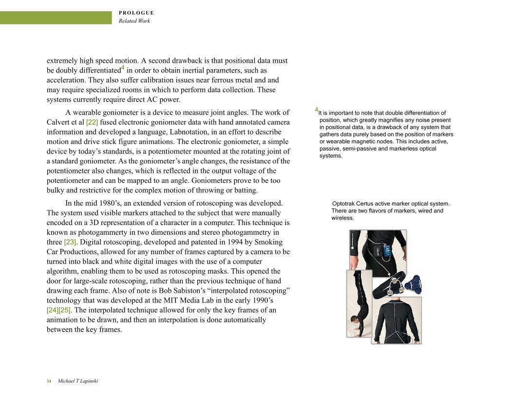
Optotrak Certus active marker optical system. There are two flavors of markers, wired and wireless.
In the mid 1980’s, an extended version of rotoscoping was developed. The system used visible markers attached to the subject that were manually encoded on a 3D representation of a character in a computer. This technique is known as photogammerty in two dimensions and stereo photogammetry in three [23]. Digital rotoscoping, developed and patented in 1994 by Smoking Car Productions, allowed for any number of frames captured by a camera to be turned into black and white digital images with the use of a computer algorithm, enabling them to be used as rotoscoping masks. This opened the door for large-scale rotoscoping, rather than the previous technique of hand drawing each frame. Also of note is Bob Sabiston’s “interpolated rotoscoping” technology that was developed at the MIT Media Lab in the early 1990’s [24][25]. The interpolated technique allowed for only the key frames of an animation to be drawn, and then an interpolation is done automatically between the key frames.
34 Michael T Lapinski
. . .
. .P R O L O G U E
Related Work
2 .1 .2 Marker Based Opt ica l Trackers
During the time that these technologies were developed and actively used, optical motion capture systems were experiencing rapid development in two major areas: camera technology and algorithm development. Both were significantly aided by the rapid advances in the speed and miniaturization of integrated circuits. Additionally, optical systems became very popular in the film industry, as evidenced by the Academy Awards received by Vicon and Motion Analysis Corp. in 2005.
In 1985 it took a Sun 1 computer 17 hours to compute 8 points from 4 cameras on a 3-second trial [20] while a current Vicon system can perform the same analysis in real time. The mathematics developed for stereo photogammerty starting in the late 1800’s have been heavily optimized and extended in order to allow this.
The computation of the positions of bodily segments or objects has also been aided by the ability to capture the locations of markers faster and more precisely. Several different capture schemes have been developed: active, passive, semi-passive and markerless approaches have also been attempted and implemented.
2.1 .2 .1 Act ive Systems
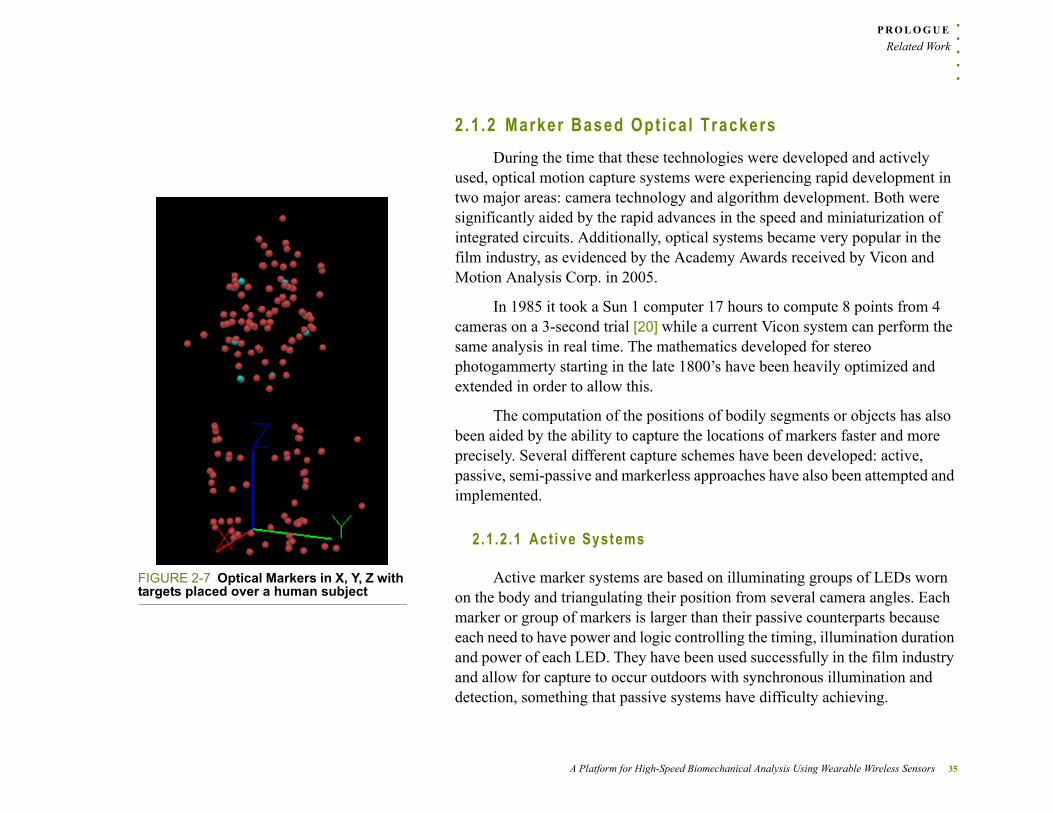
FIGURE 2-7 Optical Markers in X, Y, Z with targets placed over a human subject
Active marker systems are based on illuminating groups of LEDs worn on the body and triangulating their position from several camera angles. Each marker or group of markers is larger than their passive counterparts because each need to have power and logic controlling the timing, illumination duration and power of each LED. They have been used successfully in the film industry and allow for capture to occur outdoors with synchronous illumination and detection, something that passive systems have difficulty achieving.
A Platform for High-Speed Biomechanical Analysis Using Wearable Wireless Sensors 35
P R O L O G U E
Related Work
The first active system, SELSPOT, was developed by Selcom in 1975 and is the ancestor of the SELSPOT II system released in 1982. Northern Digital introduced the Watsmart system in the mid-1980s and the Optotrak system around 1990. Both were active systems based on linear CCD array technology that produces high resolution. These are highly accurate systems and represent a significant development that occurred in active systems after Selspot’s introduction. In 1994, Charynwood Dynamics released their Cartesian Optoelectronic Dynamic Anthropometer (CODA) active system that was successfully used in gait studies [26]. Lastly, as recently as 2012, Qualisys [10] has developed a hardwired active marker system. That sequence-coded active markers, and applied it in outdoor environments to analyze equine lameness and performance.
2.1 .2 .2 Semi-Passive Systems
Semi-Passive (or Semi-Active) systems, also labeled Time Modulated Active Marker and Semi-Passive Imperceptible Marker, also fall into the active category due to the necessity of having control software and power at each tag or marker. Prakash, a system developed by the Camera Culture Group at the MIT Media Lab, is labeled as a semi passive imperceptible marker system [27]. The scene is successfully illuminated by a series of structured IR light projections; the wearable sensors transmit via RF whether they see this illumination or not. By stitching several of these frames together, the location of the sensors can precisely and rapidly be determined. One issue is that occlusions are a problem because the sensor node must see all of the structured light to calculate the orientation and position. Considering that the received data is transmitted wirelessly back to a master host to later be integrated with
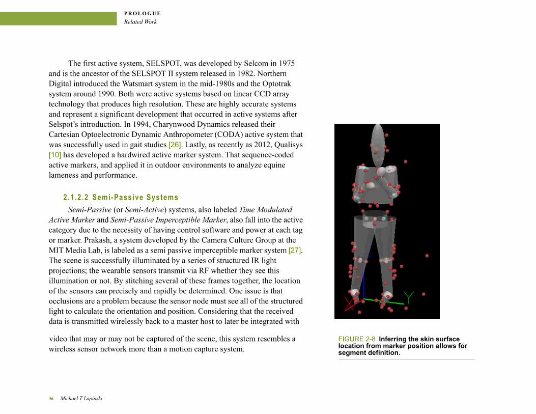
FIGURE 2-8 Inferring the skin surface location from marker position allows for segment definition.
video that may or may not be captured of the scene, this system resembles a wireless sensor network more than a motion capture system.
36 Michael T Lapinski

. . .
. .P R O L O G U E
Related Work
2.1 .2 .3 Ful ly Passive Systems
Passive marker systems are the dominant technology in motion capture; possibly due to the simplicity and flexibility of attachment and subject instrumentation. Vicon, Motion Analysis Corp and Qualysis are the major commercial players in this space and their systems are mainly used for medical research and in the film industry, with engineering (unmanned vehicles, meteorology, video game development) being the largest growing market.
The technology is based on a combination of strobing lights and cameras that work in unison to capture frames of data that show the positions of optical markers illuminated by the pulses of light. This data, taken from several different camera angles (20 or more for high speed motion), is reconstructed to build a three dimensional path for each of the markers FIGURE 2-8 . The paths of several markers can be integrated to represent segments of the human body by building an interpolated virtual ‘skin’ which the markers determine, FIGURE 2-8 . Augmenting this with anthropometric information such a diameters and lengths of segments allows inference of bone location and joint centers FIGURE 2-9 .
2 .1 .3 Iner t ia l Systems for Mot ion Capture
Inertial systems are not nearly as pervasive as optical in the medical and film communities. This is not a surprise, as the size of an inertial sensor 20 years ago made it difficult to even consider instrumentation of a human. There have been several domain-specific prototype tools for research [36][37][38] rather than fully built commercial products. These implementations are specific to a certain application and are not capable of capturing detailed motion information.
FIGURE 2-9 Skeleton defined from segment locations
Ghasemzadeh et als. work [36] uses 50Hz sampling to characterize the timing of a batter’s swing and reaffirm some of the rote rules of batting. As part of a larger body of work that addressed personal health monitoring [38],
A Platform for High-Speed Biomechanical Analysis Using Wearable Wireless Sensors 37
P R O L O G U E
Related Work
Gerasimov created Swings that Think [37]. He instrumented a bat with a gyrcoscope and accelerometer to measure the angular and acceleration parameters. Several other systems are focused on gait analysis [60], some on posture [61] and others on golf swing analysis[62]. None utilize high range sensors and instrument more then two body segments, and none attempt to reconstruct motion except for Orient-2 [63], which tracks slow moving poses over time using inertial sensing. The system has been utilized to analyze golf swings [64] and dancers of the Argentinian tango [70]. However, the range of its inertial sensors is too low to handle more extreme motion, ±300°/sec and ±6G.
As recently as 2010, work published in the Journal of Sports Engineering, whose purpose is to advance engineering in the area of sports including inertial sensors that were used to analyze tennis serves[59]. Unfortunately this work claims that, as of 2010, there does not exist a gyroscope with a range greater than ±300°/sec and the authors had to create a virtual gyroscope based on optical system marker data. While this statement is false because gyroscopes with much higher ranges were available at this time, it does indicate that the cutting edge of sports engineering is not at the cutting edge of inertial measurement unit development. It also indicates a disconnect between these two fields.
There is one main player in the commercial arena, Xsens [4], and a some lesser known companies such as Animazoo [5] and KinetiSense[6].
The Xsens system is more robust in terms of hardware, as it is comprised of gyroscopes, accelerometers and magnetometers, while the Animazoo system is based only on gyroscopes. Both systems are equipped with gyroscopes capable of sensing ±1200°/sec and the Xsens system also has a ±16G accelerometer. Both are limited to 120Hz sampling rates, which is far below the capability of optical technology.
38 Michael T Lapinski
. . .
. .P R O L O G U E
Related Work
The technology is ideally suited for studying ergonomics and gait, and while the systems claim to be usable for sports there is much to be desired with such low sampling rates, which appear to be limited by the need to have the systems operate in real time. When examining an activity that pushes the limits of human ability, such as pitching, these systems fall short. From previous work, I have observed that during an 85MPH fastball a pitcher’s hand experiences acceleration forces in excess of 110Gs and angular velocities of over 6,000 degrees/second. This is far beyond the sensing limits of the Xsens and Animazoo systems. Further, at 1000Hz sampling, the peak of the pitch consists of 3 data points or lasts 3ms. At 120Hz, each sample is taken every 8.3ms and there is a good probability that this peak would not even be detected with either existing inertial system or be extremely filtered by an anti-aliasing front-end. These simple facts dictate the need for a high-performance wearable wireless inertial sensor network.
2 .1 .4 Current P i tcher Deve lopment
In order to use a wearable sensor network on a pitcher to improve their performance, it important to understand the state of the art in molding pitchers. As alluded to in section 1.2, techniques used to develop pitchers have been passed on as rote practice from coach to coach and player to coach. Most available information is not based on any hard numbers; rules for pitching are simply preached without an explanation of why and how these rules-of-thumb were established. For example, “Coaching Pitchers” [28] states five “90 degree Rules” for pitchers that:
“A coach should be able to measure these angles with the naked eye, and by doing so he can determine whether a pitcher is mechanically sound.”
A Platform for High-Speed Biomechanical Analysis Using Wearable Wireless Sensors 39
P R O L O G U E
Related Work
Each of the rules is described briefly, with little or no explanation of what effects improper angles would have on the pitch and no discussion of how these rules were determined.
From the two sources studied by the author [28][29], the first has 23 pages dedicated to mechanics and the latter has 10. It is difficult to understand how the most important part of the pitch can be completely described with such brevity. Hence, there is a lot of opportunity in performing research that validates and explains in a quantitative manner these rules of thumb.
Along with mechanics, fatigue is another factor that is considered by coaches, because it is thought to be a contributing factor in injury. Again, the metrics associated with measuring fatigue are vague at best and the methods of controlling it are not based on numerical or scientific data. There are simply preset maximum pitch counts established. The actual count limit is not explained, again just a rule of thumb. Hence, an opportunity for future research.
It is difficult to these “rules” such as prior work because there is not much hard science behind them, however they are relevant as they are the only existing methods for player development.
2 .1 .5 Prec is ion of B iomechanica l Research
There exists a large body of biomechanical research regarding throwing. Most of it is focused on forces, torques and angular velocities experienced at the shoulder and elbow[30][31][32][33][34][35] [94][95][96] and how different mechanics effect these parameters. They do not focus on understanding what makes one pitch ‘better’ than another. Further, the relationship between injury and mechanics has also not been thoroughly explored. An in-depth review of
40 Michael T Lapinski
. . .
. .P R O L O G U E
Related Work
each prior study would be a dissertation in itself. The focus in this section is different.
5Thank you Mr.Kepple In order to understand the precision of a wearable sensor network, it is important to focus on the precision of the velocities and accelerations used to perform the biomechanical analysis in these studies and compare both systems. Most examined literature leverages techniques developed by Feltner and Dapena [39][40][41][42] to calculate joint forces and torques in the upper body, with the target activity being overhead throwing or swinging. Unfortunately, sources of error are not discussed in any significant detail in these papers.
While there is not much information regarding acceleration and velocity precision in known literature, there are four factors that should be considered when trying to answer the question of how good optical systems are5.
2.1 .5 .1 Tracking Marker and the Under ly ing Skeleton
Characterizing how well markers on the surface of the skin represent the underlying skeleton and understanding errors present due to soft tissue artifacts (STA’s)(markers moving on the skin surface) has been widely studied[43][44][45][46][47].
The general consensus is that even with current inexpensive technology [44], marker location is within a ±0.5mm difference in precision between systems using a man made calibration rig. With smaller capture volumes (180 x 180 x 150 mm3) the accuracy is as good as 63±5μm and precision of 15μm[47] using a robotic test apparatus. It is important to note that these studies were all performed with slow moving trials.
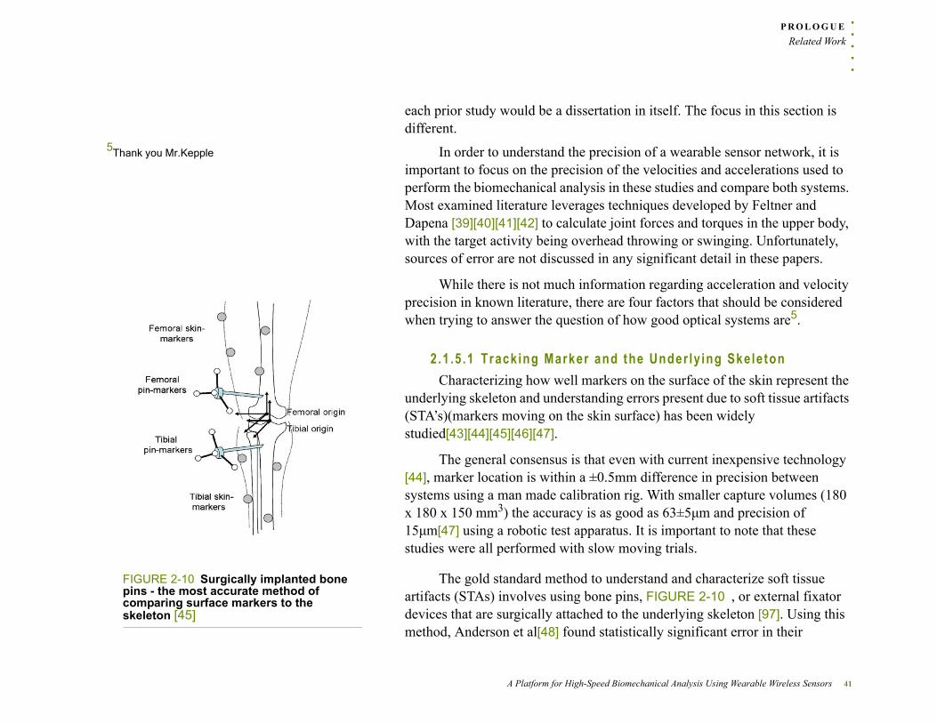
FIGURE 2-10 Surgically implanted bone pins - the most accurate method of comparing surface markers to the skeleton [45]
The gold standard method to understand and characterize soft tissue artifacts (STAs) involves using bone pins, FIGURE 2-10 , or external fixator devices that are surgically attached to the underlying skeleton [97]. Using this method, Anderson et al[48] found statistically significant error in their
A Platform for High-Speed Biomechanical Analysis Using Wearable Wireless Sensors 41
P R O L O G U E
Related Work
measurements of joint angle of the knee. However, in reality the error was about 1 degree of the
angular measurement, which is not significant for studies of gait. Again, the caveat with this work is that the trails studied were slow walking gait.
While not close in terms of angular velocity and acceleration, running with bone pins has been studied by Reinschmidt et al [46] with drastically different results. Errors relative to the range of motion during running stance were 21% for flexion/extension, 63% for internal/external rotation and 70% for abduction/adduction.
2.1 .5 .2 Marker Set Used
In order to reduce error due to STAs, different configurations and placement points for marker sets have been studied and optimized. Much of this work relates to gait[49][50], some relates to the entire skeleton [51]. The conclusions from this research is that the correct marker set makes the estimation of the joint centers and segment orientation more accurate.
Upper body marker sets for the specific purpose of throwing [71][72][73]have been developed. The primary focus of this research is to mitigate soft tissues artifacts by placing markers on bony prominences.
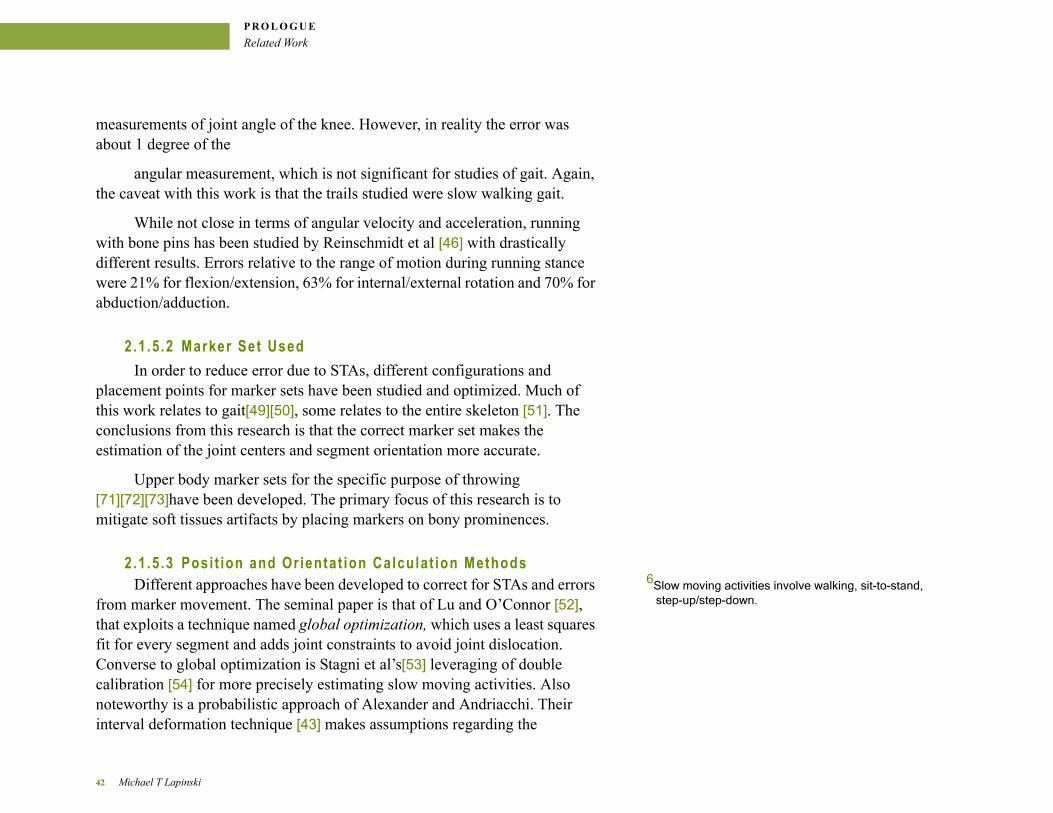
2.1 .5 .3 Posi t ion and Or ientat ion Calculat ion Methods6Slow moving activities involve walking, sit-to-stand,
step-up/step-down.Different approaches have been developed to correct for STAs and errors
from marker movement. The seminal paper is that of Lu and O’Connor [52], that exploits a technique named global optimization, which uses a least squares fit for every segment and adds joint constraints to avoid joint dislocation. Converse to global optimization is Stagni et al’s[53] leveraging of double calibration [54] for more precisely estimating slow moving activities. Also noteworthy is a probabilistic approach of Alexander and Andriacchi. Their interval deformation technique [43] makes assumptions regarding the
42 Michael T Lapinski
. . .
. .P R O L O G U E
Related Work
performed activities, and uses this information to provide a better estimate of position and orientation. While there is no single ‘correct’ method, the general takeaway is that the methodology used to accommodate for skin tissue artifacts and how data is processed when estimating orientation and position will effect the accuracy of estimation.
2.1 .5 .4 Iner t ia l Parameter Est imat ion
Directly related to the estimation of position and orientation is calculating first and second order derivatives to obtain velocities and accelerations. Any errors present in position estimation will be magnified and manifest themselves as noise when these derivatives are taken.
Inertial models of the human body[55][56] have been developed along with methods of determining angular momentum[57][58] by Yeadon. As mentioned in the start of section 2.1.5, existing literature does not attempt to quantify error in moment and acceleration calculations. This does make sense because the goal of researchers studying gait and human movement is not to research the quality of their measurement equipment, but to study human movement. They appear to simply accept the best tools available and put them to use, but they need to understand the limits of accuracy.
One of the main motivations in utilizing inertial sensors is because they measure acceleration and angular velocity, currently inferred via derivatives, directly. Although inferring absolute position and/or joint angles with inertial systems involves its own complications (discussed in Section 10.2.3), thorough calibration virtually eliminates error in inertial data streams and allows for kinetic calculation that is much more accurate and precise than optical systems.
A Platform for High-Speed Biomechanical Analysis Using Wearable Wireless Sensors 43

P R O L O G U E
Related Work
44 Michael T Lapinski

. . .
. .TA X O N O M Y, H I G H L E V E L A R C H I T E C T U R E & K I N E T I C M O D E L
TAXONOMY, HIGH
LEVEL ARCHITECTURE
. . . .
. . . . . . . . . . . . . . . . . . . . . . . . . . . . . . . . . . . . . .& KINETIC MODEL
Y ou say toe-may-toe, I say toe-mah-toe. I say poh-tay-toe, you say poh-tah-toe.
- George & Ira Gershwin
This chapter contains the naming conventions used and stitches these together to define high level system concepts to allow for a better understanding of the overall system. The system architecture is presented at high-level along with the upper body model used to represent motion.
A Platform for High-Speed Biomechanical Analysis Using Wearable Wireless Sensors 45

TA X O N O M Y, H I G H L E V E L A R C H I T E C T U R E & K I N E T I C M O D E L
Taxonomy
. . . . . . . . . . . . . . . . . . . . . . . . . . . . . . . . . . . . . . . . . . . . . . . . . . . . . . . . . . .3 . 1 T A X O N O M Y
Mean or average? Standard deviation or sigma? Stochastic or random? Integration or summation? Sampled data or observation? Different branches of science define the same or similar concepts using different words and very rarely acknowledge it or attempt to rectify them. This leads to confusion for novices who are attempting to learn a new field.
This dissertation also has its own, albeit small, taxonomy and the purpose of this section is to define it and describe it’s analogs in existing scientific or practiced fields.
3.1 .0 .1 Player
The term player is used to describe the person that the sensor network is applied to. Its analog in the in medical research is subject The goal of the system is to analyze athletes and, until now, each athlete has been a player on a baseball team, hence the name player. Each player’s definition consists of standard biometric information:
1 First Name
2 Last Name
3 Player ID - unique player identifier
4 Age
5 Height
6 Weight
7 Player Number
8 Throwing Hand (Left or Right)
9 Batting Hand (Left or Right)
46 Michael T Lapinski

. . .
. .TA X O N O M Y, H I G H L E V E L A R C H I T E C T U R E & K I N E T I C M O D E L
Taxonomy
10 Player Type - Batter or Pitcher
11 Has had previous shoulder pain?
12 Has had previous shoulder surgery?
In order to perform accurate biomechanical analysis, anthropometric data is also recorded for each player and measured using a flexible tape measure between manually identified biomechanical landmarks. At this level, data consists of measurements that do not change greatly over time for a player:
13 Forearm Length - lateral epicondyle to radial styloid
14 Upper Arm Length - lateral acromion to lateral epicondyle
15 Chest Width - sternal notch to lateral acromion
16 Pelvis Width
17 Elbow Circumference
18 Wrist Circumference
As part of the experimental process all of these items are recorded in a logbook at the time of player instrumentation and entered into a database at a later time. Each player has a collection of sessions (Section 3.1.0.2) associated with themselves.
3.1 .0 .2 Session
Each time a player is instrumented and data is gathered, a new session is defined. Asession is a collection of gestures (Section 3.1.0.3). The concept of the session does not have an analog in other fields, but is important because and each time a player is instrumented, sensor placement and certain anthropometric measurements may be different between sessions. The need to store this information dictated the definition of session. Each session contains general session information:
A Platform for High-Speed Biomechanical Analysis Using Wearable Wireless Sensors 47

TA X O N O M Y, H I G H L E V E L A R C H I T E C T U R E & K I N E T I C M O D E L
Taxonomy
1 Session Name
2 Session ID - unique session identifier
3 Hand Node ID
4 Forearm Node ID
5 Upper Arm Node ID
6 Chest Node ID
7 Waist Node ID
As mentioned previously, each session also contains anthropometric data and node location information that changes from session to session:7
7Future applications of this technology may use more specific technology to measure node location.
8 Radial Styloid to Hand Node Location
9 Lateral Epicondyle to Forearm Node Location
10 Lateral Acromion to Upper Arm Node Location
11 Sternal Notch to Chest Node Location
12 Chest Node Location to Waist Node Location
13 Arm Circumference
14 Chest Circumference
15 Waist Circumference
16 Waist Node to Floor Distance
17 Stomach to Lower Back Thickness
18 Chest Thickness
19 Depth from Stomach to Chest - (Stomach to Lower Back Thickness)
minus (Chest Thickness)
Additionally, for batting, two additional measurements are performed:
20 Bat Length
48 Michael T Lapinski
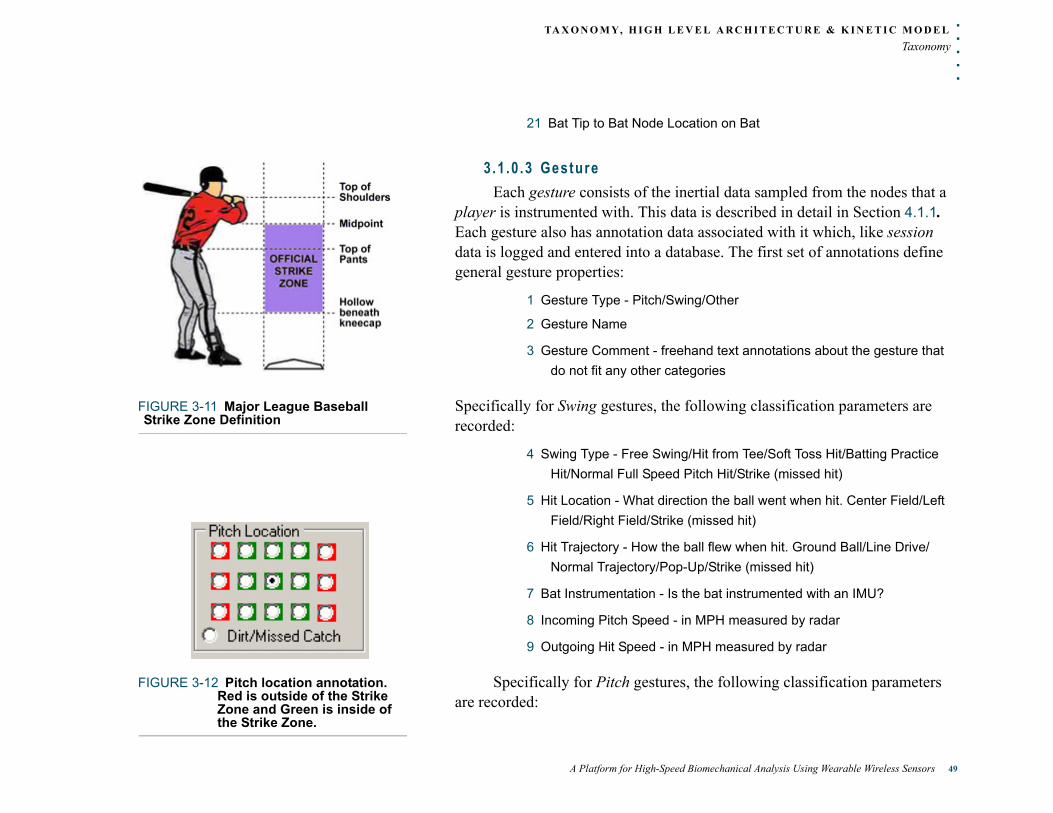
. . .
. .TA X O N O M Y, H I G H L E V E L A R C H I T E C T U R E & K I N E T I C M O D E L
Taxonomy
21 Bat Tip to Bat Node Location on Bat
3.1 .0 .3 Gesture
Each gesture consists of the inertial data sampled from the nodes that a player is instrumented with. This data is described in detail in Section 4.1.1. Each gesture also has annotation data associated with it which, like session data is logged and entered into a database. The first set of annotations define general gesture properties:
1 Gesture Type - Pitch/Swing/Other
2 Gesture Name
3 Gesture Comment - freehand text annotations about the gesture that
do not fit any other categories
FIGURE 3-11 Major League Baseball Strike Zone Definition
Specifically for Swing gestures, the following classification parameters are recorded:
4 Swing Type - Free Swing/Hit from Tee/Soft Toss Hit/Batting Practice
Hit/Normal Full Speed Pitch Hit/Strike (missed hit)
5 Hit Location - What direction the ball went when hit. Center Field/Left
Field/Right Field/Strike (missed hit)
6 Hit Trajectory - How the ball flew when hit. Ground Ball/Line Drive/
Normal Trajectory/Pop-Up/Strike (missed hit)
7 Bat Instrumentation - Is the bat instrumented with an IMU?
8 Incoming Pitch Speed - in MPH measured by radar
9 Outgoing Hit Speed - in MPH measured by radar
FIGURE 3-12 Pitch location annotation. Red is outside of the Strike Zone and Green is inside of the Strike Zone.
Specifically for Pitch gestures, the following classification parameters are recorded:
A Platform for High-Speed Biomechanical Analysis Using Wearable Wireless Sensors 49
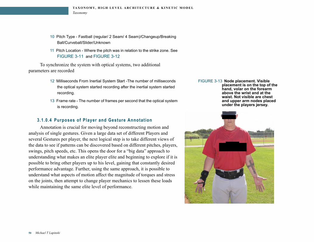
TA X O N O M Y, H I G H L E V E L A R C H I T E C T U R E & K I N E T I C M O D E L
Taxonomy
10 Pitch Type - Fastball (regular/ 2 Seam/ 4 Seam)/Changeup/Breaking
Ball/Curveball/Slider/Unknown
11 Pitch Location - Where the pitch was in relation to the strike zone. See
FIGURE 3-11 and FIGURE 3-12
To synchronize the system with optical systems, two additional parameters are recorded
FIGURE 3-13 Node placement. Visible placement is on the top of the hand, volar on the forearm above the wrist and at the waist. Not visible are chest and upper arm nodes placed under the players jersey.
12 Milliseconds From Inertial System Start -The number of milliseconds
the optical system started recording after the inertial system started
recording.
13 Frame rate - The number of frames per second that the optical system
is recording.
3.1 .0 .4 Purposes of P layer and Gesture Annotat ion
Annotation is crucial for moving beyond reconstructing motion and analysis of single gestures. Given a large data set of different Players and several Gestures per player, the next logical step is to take different views of the data to see if patterns can be discovered based on different pitches, players, swings, pitch speeds, etc. This opens the door for a “big data” approach to understanding what makes an elite player elite and beginning to explore if it is possible to bring other players up to his level, gaining that constantly desired performance advantage. Further, using the same approach, it is possible to understand what aspects of motion affect the magnitude of torques and stress on the joints, then attempt to change player mechanics to lessen these loads while maintaining the same elite level of performance.
50 Michael T Lapinski
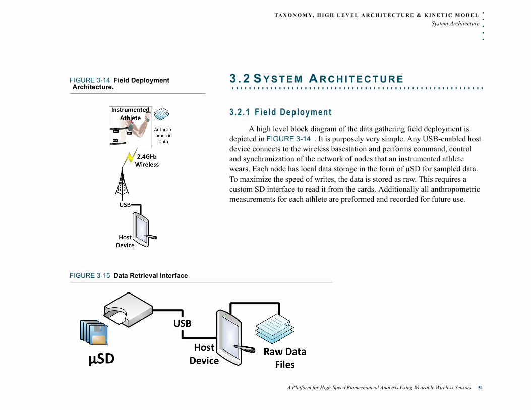
. . .
. .TA X O N O M Y, H I G H L E V E L A R C H I T E C T U R E & K I N E T I C M O D E L
System Architecture
FIGURE 3-14 Field Deployment Architecture. . . . . . . . . . . . . . . . . . . . . . . . . . . . . . . . . . . . . . . . . . . . . . . . . . . . . . . . . . . .3 . 2 S Y S T E M A R C H I T E C T U R E
3.2 .1 F ie ld Deployment
A high level block diagram of the data gathering field deployment is depicted in FIGURE 3-14 . It is purposely very simple. Any USB-enabled host device connects to the wireless basestation and performs command, control and synchronization of the network of nodes that an instrumented athlete wears. Each node has local data storage in the form of µSD for sampled data. To maximize the speed of writes, the data is stored as raw. This requires a custom SD interface to read it from the cards. Additionally all anthropometric measurements for each athlete are preformed and recorded for future use.
FIGURE 3-15 Data Retrieval Interface
A Platform for High-Speed Biomechanical Analysis Using Wearable Wireless Sensors 51
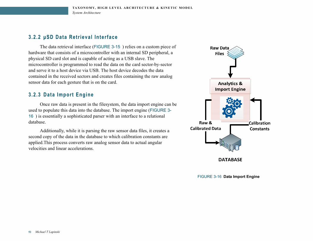
TA X O N O M Y, H I G H L E V E L A R C H I T E C T U R E & K I N E T I C M O D E L
System Architecture
3 .2 .2 µSD Data Ret r ieva l In ter face
The data retrieval interface (FIGURE 3-15 ) relies on a custom piece of hardware that consists of a microcontroller with an internal SD peripheral, a physical SD card slot and is capable of acting as a USB slave. The microcontroller is programmed to read the data on the card sector-by-sector and serve it to a host device via USB. The host device decodes the data contained in the received sectors and creates files containing the raw analog sensor data for each gesture that is on the card.
3 .2 .3 Data Impor t Engine
Once raw data is present in the filesystem, the data import engine can be used to populate this data into the database. The import engine (FIGURE 3-16 ) is essentially a sophisticated parser with an interface to a relational database.
Additionally, while it is parsing the raw sensor data files, it creates a second copy of the data in the database to which calibration constants are applied.This process converts raw analog sensor data to actual angular velocities and linear accelerations.
FIGURE 3-16 Data Import Engine
52 Michael T Lapinski
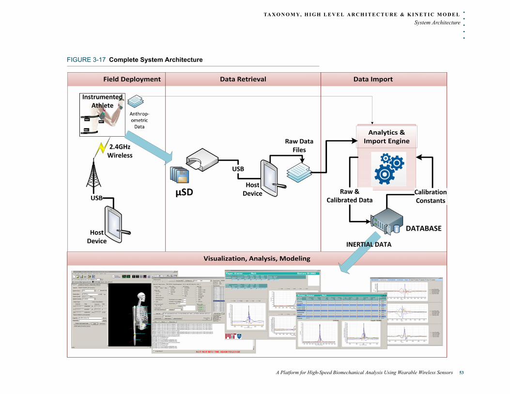
. . .
. .TA X O N O M Y, H I G H L E V E L A R C H I T E C T U R E & K I N E T I C M O D E L
System Architecture
FIGURE 3-17 Complete System Architecture
A Platform for High-Speed Biomechanical Analysis Using Wearable Wireless Sensors 53
TA X O N O M Y, H I G H L E V E L A R C H I T E C T U R E & K I N E T I C M O D E L
Physical (Kinematic) Model
3 .2 .4 V isua l iza t ion , Ana lys is and Model ing
The entire system is presented in FIGURE 3-17 , where a persistent data store containing classified Player, Session and Gesture inertial and anthropometric data opens the door to building player-and-gesture-specific-models and performing medically significant research. An interface has been built for C/C++, Matlab and Visual Basic in order to retrieve, slice, dice and visualize data any way that is imaginable. The granularity of the data can be per athlete, per session, per gesture, per segment, per sensor and even per sensed axis. The only limiting factor is the capability and imagination of the model builder.
. . . . . . . . . . . . . . . . . . . . . . . . . . . . . . . . . . . . . . . . . . . . . . . . . . . . . . . . . . .3 . 3 P H Y S I C A L ( K I N E M A T I C) M O D E L
8The evolution of node attachment to player’s bodies is covered in-depth in Section 7.1, here we will briefly describe node placement to set the context for understanding the physical model. As visible in FIGURE 3-13 , nodes are attached to the hand, forearm and waist. Two nodes are not visible in the figure, as these are attached to the upper arm and on the chest.
At the opposite end of the spectrum from the Player, Session and Gesture taxonomy is the physical kinematic model that is driven by data from the sensor network. In order to accommodate different players of different sizes, this physical model cannot be statically defined. Also, as described in Section 3.1.0.2, the placement of nodes between sessions differs and the representation of this placement8 must also be encoded into the model.
3 .3 .1 Coord inate Systems
Coordinate systems are visible in FIGURE 3-19 . The Z axis is Blue and positive is up. The Y axis is green and positive is forward out of the chest. The X axis is red and positive extends out of the right arm. For rotations, the right-hand rule is used to define positive and negative rotation. The origin of each segment’s coordinate system is placed at the segment’s center of mass. In
54 Michael T Lapinski
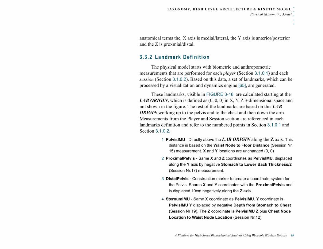
. . .
. .TA X O N O M Y, H I G H L E V E L A R C H I T E C T U R E & K I N E T I C M O D E L
Physical (Kinematic) Model
anatomical terms the, X axis is medial/lateral, the Y axis is anterior/posterior and the Z is proxmial/distal.
3 .3 .2 Landmark Def in i t ion
The physical model starts with biometric and anthropometric measurements that are performed for each player (Section 3.1.0.1) and each session (Section 3.1.0.2). Based on this data, a set of landmarks, which can be processed by a visualization and dynamics engine [65], are generated.
These landmarks, visible in FIGURE 3-18 are calculated starting at the LAB ORIGIN, which is defined as (0, 0, 0) in X, Y, Z 3-dimensional space and not shown in the figure. The rest of the landmarks are based on this LAB ORIGIN working up to the pelvis and to the chest and then down the arm. Measurements from the Player and Session section are referenced in each landmarks definition and refer to the numbered points in Section 3.1.0.1 and Section 3.1.0.2.
1 PelvisIMU - Directly above the LAB ORIGIN along the Z axis. This
distance is based on the Waist Node to Floor Distance (Session Nr.
15) measurement. X and Y locations are unchanged (0, 0)
2 ProximalPelvis - Same X and Z coordinates as PelvisIMU, displaced
along the Y axis by negative Stomach to Lower Back Thickness/2
(Session Nr.17) measurement.
3 DistalPelvis - Construction marker to create a coordinate system for
the Pelvis. Shares X and Y coordinates with the ProximalPelvis and
is displaced 10cm negatively along the Z axis.
4 SternumIMU - Same X coordinate as PelvisIMU. Y coordinate is
PelvisIMU Y displaced by negative Depth from Stomach to Chest
(Session Nr 19). The Z coordinate is PelvisIMU Z plus Chest Node
Location to Waist Node Location (Session Nr.12).
A Platform for High-Speed Biomechanical Analysis Using Wearable Wireless Sensors 55
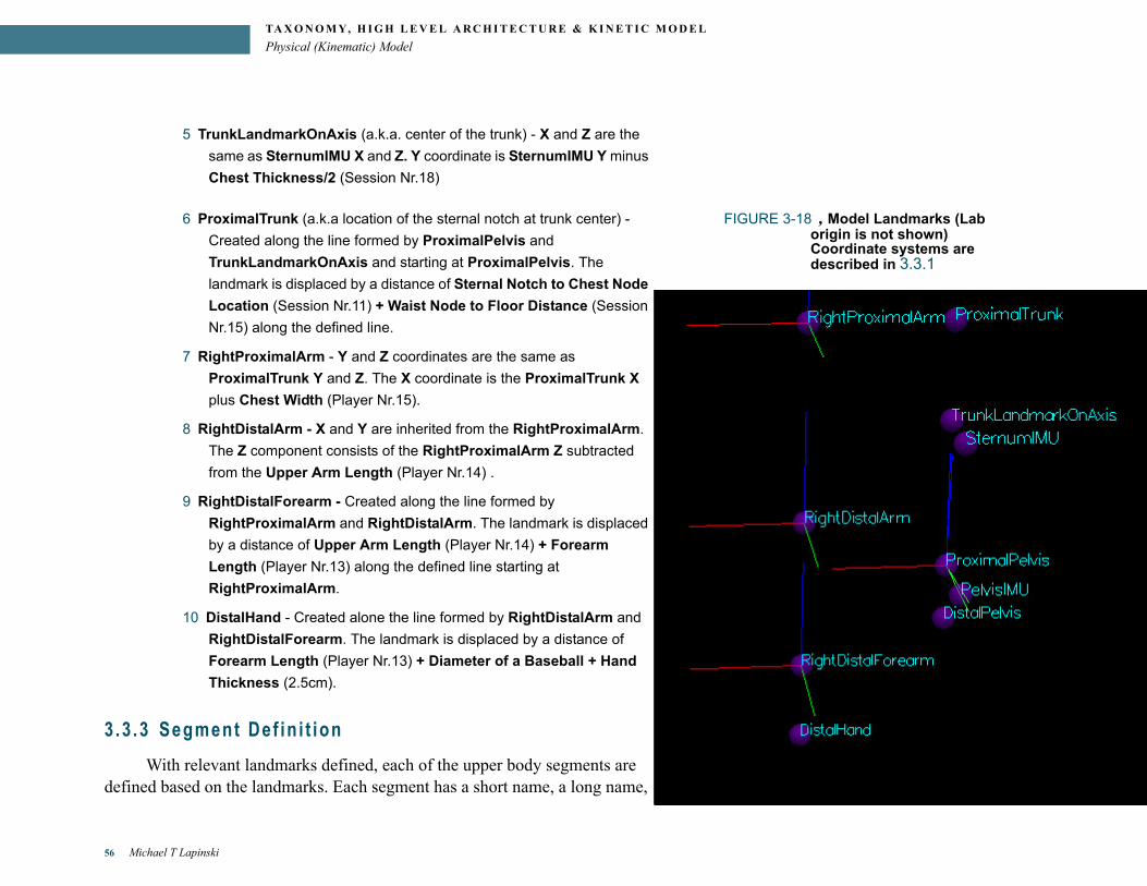
TA X O N O M Y, H I G H L E V E L A R C H I T E C T U R E & K I N E T I C M O D E L
Physical (Kinematic) Model
5 TrunkLandmarkOnAxis (a.k.a. center of the trunk) - X and Z are the
same as SternumIMU X and Z. Y coordinate is SternumIMU Y minus
Chest Thickness/2 (Session Nr.18)
FIGURE 3-18 , Model Landmarks (Lab origin is not shown) Coordinate systems are described in 3.3.1
6 ProximalTrunk (a.k.a location of the sternal notch at trunk center) -
Created along the line formed by ProximalPelvis and
TrunkLandmarkOnAxis and starting at ProximalPelvis. The
landmark is displaced by a distance of Sternal Notch to Chest Node
Location (Session Nr.11) + Waist Node to Floor Distance (Session
Nr.15) along the defined line.
7 RightProximalArm - Y and Z coordinates are the same as
ProximalTrunk Y and Z. The X coordinate is the ProximalTrunk X
plus Chest Width (Player Nr.15).
8 RightDistalArm - X and Y are inherited from the RightProximalArm.
The Z component consists of the RightProximalArm Z subtracted
from the Upper Arm Length (Player Nr.14) .
9 RightDistalForearm - Created along the line formed by
RightProximalArm and RightDistalArm. The landmark is displaced
by a distance of Upper Arm Length (Player Nr.14) + Forearm
Length (Player Nr.13) along the defined line starting at
RightProximalArm.
10 DistalHand - Created alone the line formed by RightDistalArm and
RightDistalForearm. The landmark is displaced by a distance of
Forearm Length (Player Nr.13) + Diameter of a Baseball + Hand
Thickness (2.5cm).
3 .3 .3 Segment Def in i t ion
With relevant landmarks defined, each of the upper body segments are defined based on the landmarks. Each segment has a short name, a long name,
56 Michael T Lapinski
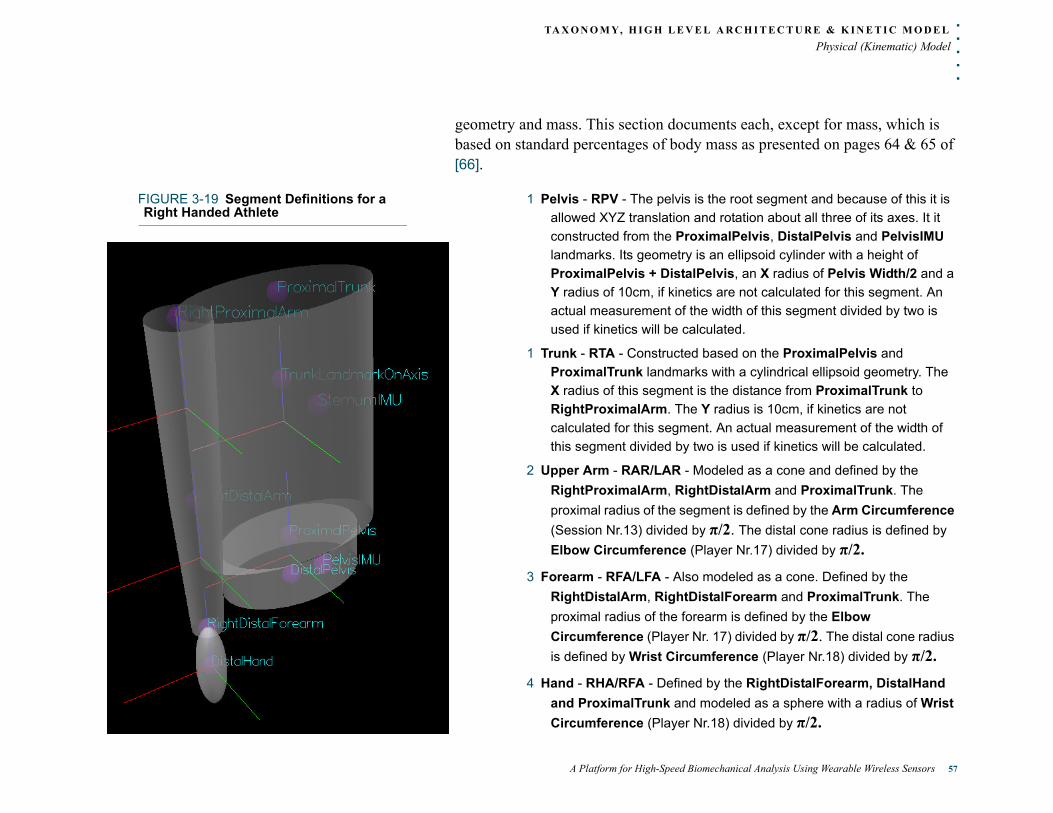
. . .
. .TA X O N O M Y, H I G H L E V E L A R C H I T E C T U R E & K I N E T I C M O D E L
Physical (Kinematic) Model
geometry and mass. This section documents each, except for mass, which is based on standard percentages of body mass as presented on pages 64 & 65 of [66].
FIGURE 3-19 Segment Definitions for a Right Handed Athlete
1 Pelvis - RPV - The pelvis is the root segment and because of this it is
allowed XYZ translation and rotation about all three of its axes. It it
constructed from the ProximalPelvis, DistalPelvis and PelvisIMU
landmarks. Its geometry is an ellipsoid cylinder with a height of
ProximalPelvis + DistalPelvis, an X radius of Pelvis Width/2 and a
Y radius of 10cm, if kinetics are not calculated for this segment. An
actual measurement of the width of this segment divided by two is
used if kinetics will be calculated.
1 Trunk - RTA - Constructed based on the ProximalPelvis and
ProximalTrunk landmarks with a cylindrical ellipsoid geometry. The
X radius of this segment is the distance from ProximalTrunk to
RightProximalArm. The Y radius is 10cm, if kinetics are not
calculated for this segment. An actual measurement of the width of
this segment divided by two is used if kinetics will be calculated.
2 Upper Arm - RAR/LAR - Modeled as a cone and defined by the
RightProximalArm, RightDistalArm and ProximalTrunk. The
proximal radius of the segment is defined by the Arm Circumference
(Session Nr.13) divided by π/2. The distal cone radius is defined by
Elbow Circumference (Player Nr.17) divided by π/2.
3 Forearm - RFA/LFA - Also modeled as a cone. Defined by the
RightDistalArm, RightDistalForearm and ProximalTrunk. The
proximal radius of the forearm is defined by the Elbow
Circumference (Player Nr. 17) divided by π/2. The distal cone radius
is defined by Wrist Circumference (Player Nr.18) divided by π/2.
4 Hand - RHA/RFA - Defined by the RightDistalForearm, DistalHand
and ProximalTrunk and modeled as a sphere with a radius of Wrist
Circumference (Player Nr.18) divided by π/2.
A Platform for High-Speed Biomechanical Analysis Using Wearable Wireless Sensors 57

TA X O N O M Y, H I G H L E V E L A R C H I T E C T U R E & K I N E T I C M O D E L
Physical (Kinematic) Model
3 .3 .4 Jo in t Def in i t ion
There are four joints for the upper body model. Each is modeled as a ball and socket with no possibility of translation. The means that each joint has 3 DOF, but does not mean that the joint cannot translate in 3 dimensional space. Joints and segment translation is driven by the root segment, the Pelvis.
Further, each joint has a given order of rotation angle application. The joints and their rotation sequences are as follows:
9this is based on the recommendations of the International Shoulder Group [67][68]
1 Spine Joint - for lack of a better name, the joint between the Pelvis
and Trunk is named the Spine Joint. It’s Euler rotation sequence is
XYZ
2 Shoulder Joint - this is the joint between the Trunk and Upper Arm
and has an Euler sequence of ZYZ9.
3 Elbow Joint - the joint between the Upper Arm and Forearm with an
Euler sequence of XYZ.
4 Wrist Joint - the joint between the Forearm and Hand segments. Also
with an Euler sequence of XYZ.
58 Michael T Lapinski
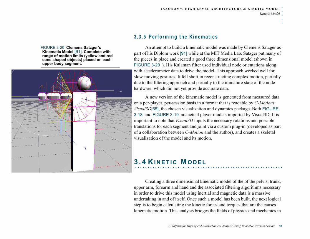
. . .
. .TA X O N O M Y, H I G H L E V E L A R C H I T E C T U R E & K I N E T I C M O D E L
Kinetic Model
3 .3 .5 Per forming the K inemat ics
FIGURE 3-20 Clemens Satzger’s Kinematic Model [91]. Complete with range of motion limits (yellow and red cone shaped objects) placed on each upper body segment.
An attempt to build a kinematic model was made by Clemens Satzger as part of his Diplom work [91] while at the MIT Media Lab. Satzger put many of the pieces in place and created a good three dimensional model (shown in FIGURE 3-20 ). His Kalaman filter used individual node orientations along with accelerometer data to drive the model. This approach worked well for slow-moving gestures. It fell short in reconstructing complex motion, partially due to the filtering approach and partially to the immature state of the node hardware, which did not yet provide accurate data.
A new version of the kinematic model is generated from measured data on a per-player, per-session basis in a format that is readable by C-Motions Visual3D[65], the chosen visualization and dynamics package. Both FIGURE 3-18 and FIGURE 3-19 are actual player models imported by Visual3D. It is important to note that Visual3D inputs the necessary rotations and possible translations for each segment and joint via a custom plug-in (developed as part of a collaboration between C-Motion and the author), and creates a skeletal visualization of the model and its motion.
. . . . . . . . . . . . . . . . . . . . . . . . . . . . . . . . . . . . . . . . . . . . . . . . . . . . . . . . . . .3 . 4 K I N E T I C M O D E L
Creating a three dimensional kinematic model of the of the pelvis, trunk, upper arm, forearm and hand and the associated filtering algorithms necessary in order to drive this model using inertial and magnetic data is a massive undertaking in and of itself. Once such a model has been built, the next logical step is to begin calculating the kinetic forces and torques that are the causes kinematic motion. This analysis bridges the fields of physics and mechanics in
A Platform for High-Speed Biomechanical Analysis Using Wearable Wireless Sensors 59
TA X O N O M Y, H I G H L E V E L A R C H I T E C T U R E & K I N E T I C M O D E L
Kinetic Model
a non-trivial manner because all calculations must be performed in three dimensions and the underlying mechanical model has multiple rigid bodies and joints. Fortunately for this author, there exist systems, built to process optical system data, that implement and execute the kinetic modeling necessary for obtaining the desired forces and torques.
One of these is Visual3D from C-Motion Incorporated [65], who, as previously mentioned, is a collaborator on this project in three ways. Tom Kepple, Chief Science Officer at C-Motion, is a biomechanics expert, an invaluable mentor for all things optical and biomechanical and also a reader on the committee for this dissertation. Second, as described in Section 3.3.5, the physical model is generated in a manner that is readable by Visual3D and is driven via a custom plug-in. The last facet of the collaboration is to pair Visual3D’s proprietary kinetics engine with the inertial data gathered from each instrumented segment and perform kinetic calculations.
Internally, and because it is built to process X, Y, Z marker positions, Visual3D calculates its own angular velocities, along with angular and linear accelerations based on the markers and ‘feeds’ these into its kinetics engine. In order to use inertial data to ‘feed’ this model, Visual3D has been modified to import such data from our database and analytics engine via the custom plug-in. Once this data is paired with kinematic data, the entire suite of Visual3D’s kinetics algorithms are available for generating results. It is important to note that in keeping with the spirit of keeping athletes in their native environment while studying them, a goal of this work is to keep the medical researcher in their native environment when acquiring research data. Using the familiar and well known Visual3D environment as the interface researchers will interact with aligns itself ideally with this philosophy.
60 Michael T Lapinski
. . .
. .T H E TA N G I B L E
. . . .
. . . . . . . . . . . . . . . . . . . . . . . . . . . . . . . . . . . . . .THE TANGIBLE
t
The combination of various tangible electronic parts forms the inertial sensing node into an instrument used to measure various motion parameters. This chapter details the instrument that has been tuned to capture the symphony of forces experienced by an athlete’s body as he plays.
A Platform for High-Speed Biomechanical Analysis Using Wearable Wireless Sensors 61

T H E TA N G I B L E
Wireless Inertial Measurement Node
4 . 1 W I R E L E S S I N E R T I A L M E A S U R E M E N T
. . . . . . . . . . . . . . . . . . . . . . . . . . . . . . . . . . . . . . . . . . . . . . . . . . . . . . . . . . .N O D E
The wireless inertial measurement node consists of four physical parts: the main board, two identical high range inertial daughterboards and an expansion board for wireless communication. Each node has two tiers of acceleration and angular velocity sensing capability, high and low range. The purpose of this is straightforward. A high range sensor is good at sensing very fast accelerations and angular changes but has low resolution for sensing slow moving accelerations and angular movement, whereas the low range sensors, excellent at sensing slow moving parameters, are incapable of sensing anything past their specified limits. We fuse both low and high range sensor families to attain wide dynamic range with the resolution that we require. This data fusion is non-trivial and the algorithm developed to do so is presented in Section 9.5
Our hardware has gone through 4 generations of design. The first, [74][115] was an adaptation of a low-range design used for interactive dance and only had a single range accelerometer and gyroscope set. The second, [7] was explicitly developed for sports applications and had dual-range sensors, although little onboard memory, hence streamed each collected pitch or swing to the basestation via the wireless link, which would take up to a minute. The subsequent generation [104], had virtually unlimited onboard memory via the SD card. Our final version, described here, has been designed to minimize noise, take advantage of newer and more compact sensing, support rapid data ooloading vis USB and enable higher sampling rates.
62 Michael T Lapinski
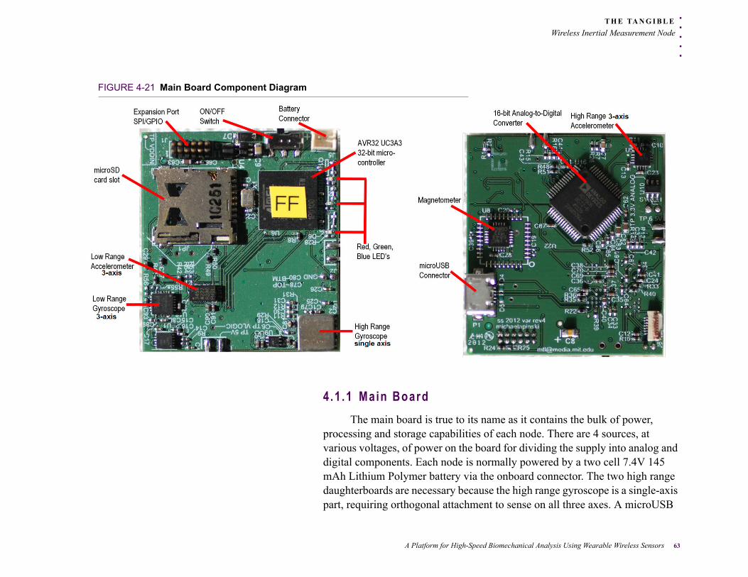
. . .
. .T H E TA N G I B L E
Wireless Inertial Measurement Node
FIGURE 4-21 Main Board Component Diagram
4.1 .1 Main Board
The main board is true to its name as it contains the bulk of power, processing and storage capabilities of each node. There are 4 sources, at various voltages, of power on the board for dividing the supply into analog and digital components. Each node is normally powered by a two cell 7.4V 145 mAh Lithium Polymer battery via the onboard connector. The two high range daughterboards are necessary because the high range gyroscope is a single-axis part, requiring orthogonal attachment to sense on all three axes. A microUSB
A Platform for High-Speed Biomechanical Analysis Using Wearable Wireless Sensors 63

T H E TA N G I B L E
Wireless Inertial Measurement Node
connector allows for wired connection of the node to a host computer for command and control of an individual node, or for the connected node to act as a basestation and perform command and control for a network of nodes. The main board has a microSD slot connected to the AVR32 microcontroller via a high speed parallel SDIO interface for storing all sampled sensor data. Additionally, the board is capable of acting as a USB master (via the microUSB port) in order to connect slave devices, such as an external hard drive for storing years of data.
The board is outfitted with a 6-channel Analog Devices AD7606 analog-to-digital converter that interfaces the AVR32 microcontroller via a Serial Peripheral Interface. The sensors connected to the AD7606 are:
1 High Range Accelerometer - The Analog Devices ADXL377 has ±200G
range, 3 orthogonal axes of sensing and analog output for each axis.
It is small and has a low power consumption, making it ideal for the
system.
2 High Range Gyroscope - A single Analog Devices ADXRS649
gyroscope is mounted on the main board. The gyroscope has a range
of ±20,000°/second and senses about its Yaw axis, making it ideal for
sensing the extreme angular velocities that athletes are capable of
producing. Its single analog output is fed into the AD7606.
The low range sensors are also mounted to the main board. These consist of:
1 Low Range Accelerometer - The Analog Devices ADXL345 running in
±16G mode has a 400kbit/s I2C digital communication interface that is
directly connected to the AVR32 microcontroller. It has 3 orthogonal
axes of sensing and is ideal for recording the slow moving
accelerations that most activity is composed of.
2 Low Range Gyrcoscope - A 3-axis Invensense IMU-3000 is configured
in ±1,000°/second mode and shares an I2C communication bus with
64 Michael T Lapinski
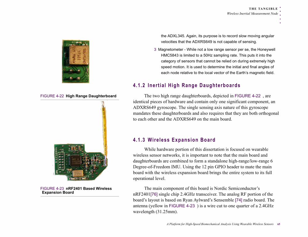
. . .
. .T H E TA N G I B L E
Wireless Inertial Measurement Node
the ADXL345. Again, its purpose is to record slow moving angular
velocities that the ADXRS649 is not capable of sensing.
3 Magnetometer - While not a low range sensor per se, the Honeywell
HMC5843 is limited to a 50Hz sampling rate. This puts it into the
category of sensors that cannot be relied on during extremely high
speed motion. It is used to determine the initial and final angles of
each node relative to the local vector of the Earth’s magnetic field.
4 .1 .2 Iner t ia l H igh Range Daughterboards
FIGURE 4-22 High Range Daughterboard The two high range daughterboards, depicted in FIGURE 4-22 , are identical pieces of hardware and contain only one significant component, an ADXRS649 gyroscope. The single sensing axis nature of this gyroscope mandates these daughterboards and also requires that they are both orthogonal to each other and the ADXRS649 on the main board.
4 .1 .3 Wire less Expansion Board
While hardware portion of this dissertation is focused on wearable wireless sensor networks, it is important to note that the main board and daughterboards are combined to form a standalone high-range/low-range 6 Degree-of-Freedom IMU. Using the 12 pin GPIO header to mate the main board with the wireless expansion board brings the entire system to its full operational level.
FIGURE 4-23 nRF2401 Based Wireless Expansion Board
The main component of this board is Nordic Semiconductor’s nRF2401[76] single chip 2.4GHz transceiver. The analog RF portion of the board’s layout is based on Ryan Aylward’s Sensemble [74] radio board. The antenna (yellow in FIGURE 4-23 ) is a wire cut to one quarter of a 2.4GHz wavelength (31.25mm).
A Platform for High-Speed Biomechanical Analysis Using Wearable Wireless Sensors 65
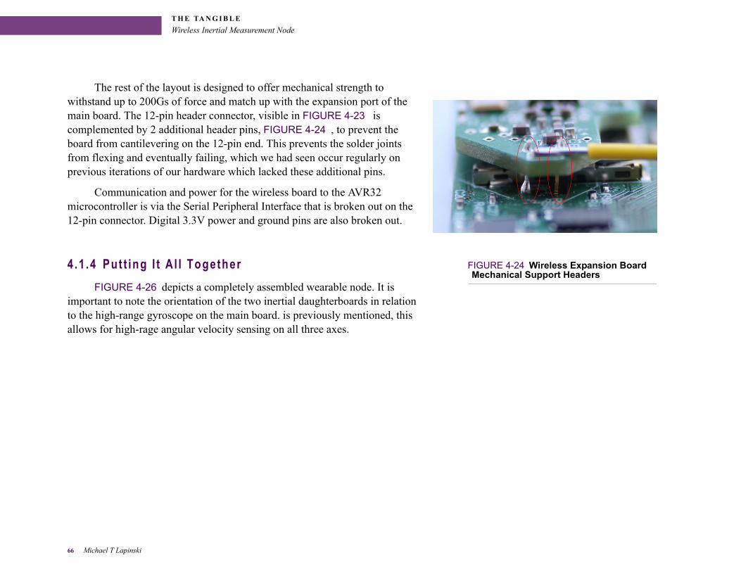
T H E TA N G I B L E
Wireless Inertial Measurement Node
The rest of the layout is designed to offer mechanical strength to withstand up to 200Gs of force and match up with the expansion port of the main board. The 12-pin header connector, visible in FIGURE 4-23 is complemented by 2 additional header pins, FIGURE 4-24 , to prevent the board from cantilevering on the 12-pin end. This prevents the solder joints from flexing and eventually failing, which we had seen occur regularly on previous iterations of our hardware which lacked these additional pins.
Communication and power for the wireless board to the AVR32 microcontroller is via the Serial Peripheral Interface that is broken out on the 12-pin connector. Digital 3.3V power and ground pins are also broken out.
FIGURE 4-24 Wireless Expansion Board Mechanical Support Headers
4 .1 .4 Put t ing I t A l l Together
FIGURE 4-26 depicts a completely assembled wearable node. It is important to note the orientation of the two inertial daughterboards in relation to the high-range gyroscope on the main board. is previously mentioned, this allows for high-rage angular velocity sensing on all three axes.
66 Michael T Lapinski
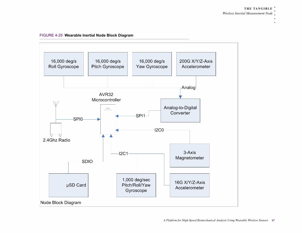
. . .
. .T H E TA N G I B L E
Wireless Inertial Measurement Node
FIGURE 4-25 Wearable Inertial Node Block Diagram
A Platform for High-Speed Biomechanical Analysis Using Wearable Wireless Sensors 67

T H E TA N G I B L E
Wireless Inertial Measurement Node
FIGURE 4-26 Complete Board Assembly
(37.5x42mm)
4 .1 .5 System Evolut ion
As mentioned earlier, the hardware presented thus far is the latest revision of a system that has been evolving to meet sensing needs and keep up with the technological evolution of available sensors. The original hardware leveraged was Ryan Aylwards 2006 Sensemble [74][115] system for instrumenting ensembles of dancers (FIGURE 4-27 ). The current revision shares only the wireless transceiver chip; all other components have been replaced with newer, smaller, less power hungry parts.
The improvement in data quality across generations has been significant. Background noise due to induced pickup from suboptimal layout and power supply conditioning was present in previous hardware revisions. The newer nodes remedy these and produce very clean data.
68 Michael T Lapinski
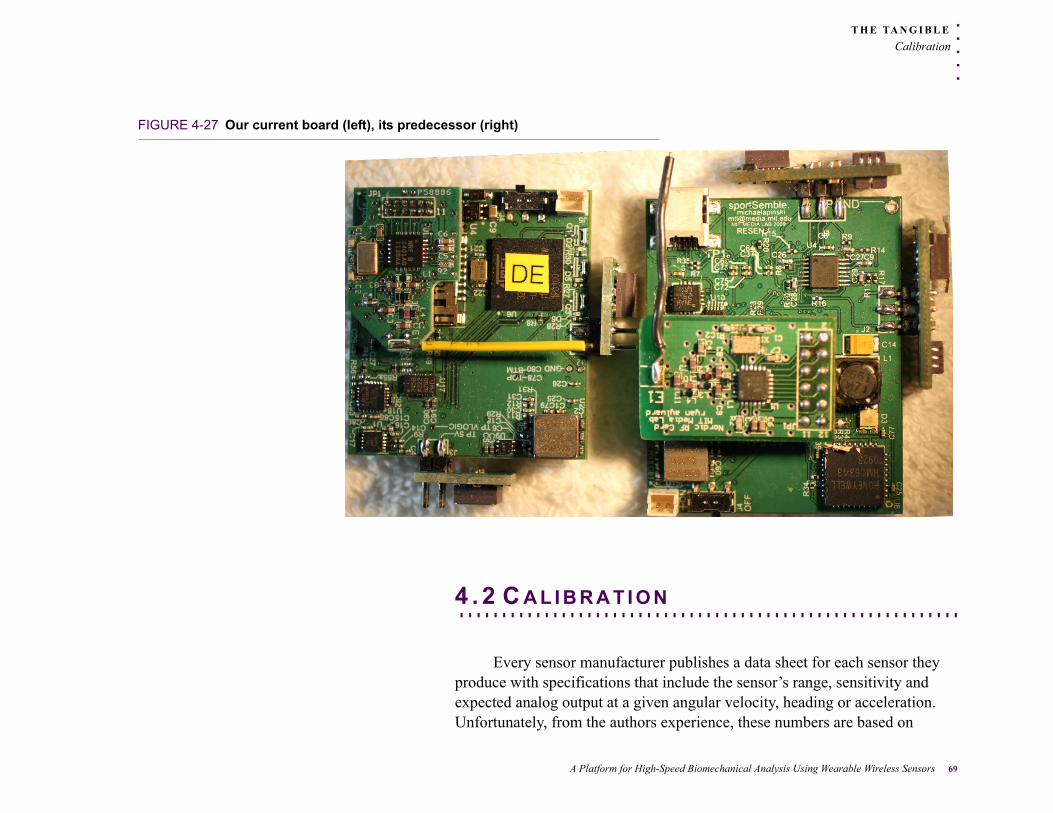
. . .
. .T H E TA N G I B L E
Calibration
FIGURE 4-27 Our current board (left), its predecessor (right)
. . . . . . . . . . . . . . . . . . . . . . . . . . . . . . . . . . . . . . . . . . . . . . . . . . . . . . . . . . .4 . 2 C A L I B R A T I O N
Every sensor manufacturer publishes a data sheet for each sensor they produce with specifications that include the sensor’s range, sensitivity and expected analog output at a given angular velocity, heading or acceleration. Unfortunately, from the authors experience, these numbers are based on
A Platform for High-Speed Biomechanical Analysis Using Wearable Wireless Sensors 69
T H E TA N G I B L E
Calibration
averages taken from several different batches of manufactured units and lack sufficient accuracy. This dictates the necessity of calibrating each axis of each sensor on each node and development of a transfer function for all sensed axes in order to ensure accurate translation from analog to inertial values. The approach used is a rotation based calibration to apply angular velocity for gyroscopes and to simulate acceleration for accelerometers. Magnetometers have their own specific calibration that involves rotation and random data input. A picture of the rig built to perform calibration is show in FIGURE 4-31 .
4 .2 .1 Rota t ion Based Cal ibra t ion
4.2 .1 .1 Gyroscopes
For gyroscopes, the rotation-based calibration concept is straightforward, because a gyroscope measures angular velocity and outputs an analog value. If the applied angular velocity is known, a transfer function can be developed to map from the analog value to the real angular velocity. Taking several samples at various angular velocities allows fitting of a curve to generate a transfer function that is generic for the specific axis of a particular sensor. Due to the inclusion of both high and low range gyroscopes on all three axes of each node, six individual gyroscope calibrations must be performed for each node built. For each axis that is calibrated a residual to a linear fit is calculated and stored, indicating the quality of the fit. For low range gyroscopes, the calibration points used were 798°/s, 600°/s, 498°/s, 402°/s, 198°/s, 0°/s, -198°/s, -402°/s, -498°/s, -600°/s and -798°/s. For the high range gyroscopes, the calibration points used were 16998°/s, 16002°/s, 12000°/s, 7998°/s, 4002°/s, 1998°/s, 0°/s, -1998°/s, -4002°/s, -7998°/s, -12000°/s, -16002°/s and -16998°/s.
70 Michael T Lapinski
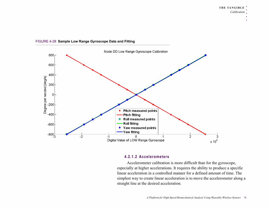
. . .
. .T H E TA N G I B L E
Calibration
FIGURE 4-28 Sample Low Range Gyroscope Data and Fitting
4.2 .1 .2 Accelerometers
Accelerometer calibration is more difficult than for the gyroscope, especially at higher accelerations. It requires the ability to produce a specific linear acceleration in a controlled manner for a defined amount of time. The simplest way to create linear acceleration is to move the accelerometer along a straight line at the desired acceleration.
A Platform for High-Speed Biomechanical Analysis Using Wearable Wireless Sensors 71
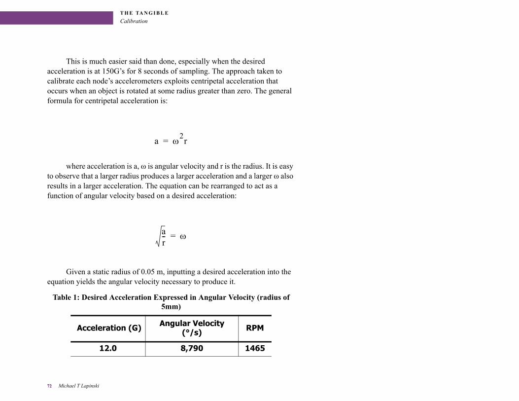
T H E TA N G I B L E
Calibration
This is much easier said than done, especially when the desired acceleration is at 150G’s for 8 seconds of sampling. The approach taken to calibrate each node’s accelerometers exploits centripetal acceleration that occurs when an object is rotated at some radius greater than zero. The general formula for centripetal acceleration is:
a 2r=
where acceleration is a, ω is angular velocity and r is the radius. It is easy to observe that a larger radius produces a larger acceleration and a larger ω also results in a larger acceleration. The equation can be rearranged to act as a function of angular velocity based on a desired acceleration:
ar-- =
Given a static radius of 0.05 m, inputting a desired acceleration into the equation yields the angular velocity necessary to produce it.
Table 1: Desired Acceleration Expressed in Angular Velocity (radius of 5mm)
Acceleration (G) Angular Velocity (°/s) RPM
12.0 8,790 1465
72 Michael T Lapinski
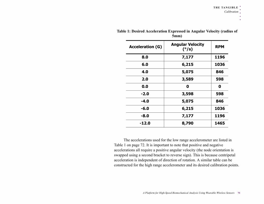
. . .
. .T H E TA N G I B L E
Calibration
The accelerations used for the low range accelerometer are listed in Table 1 on page 72. It is important to note that positive and negative accelerations all require a positive angular velocity (the node orientation is swapped using a second bracket to reverse sign). This is because centripetal acceleration is independent of direction of rotation. A similar table can be constructed for the high range accelerometer and its desired calibration points.
8.0 7,177 1196
6.0 6,215 1036
4.0 5,075 846
2.0 3,589 598
0.0 0 0
-2.0 3,598 598
-4.0 5,075 846
-6.0 6,215 1036
-8.0 7,177 1196
-12.0 8,790 1465
Table 1: Desired Acceleration Expressed in Angular Velocity (radius of 5mm)
Acceleration (G) Angular Velocity (°/s) RPM
A Platform for High-Speed Biomechanical Analysis Using Wearable Wireless Sensors 73
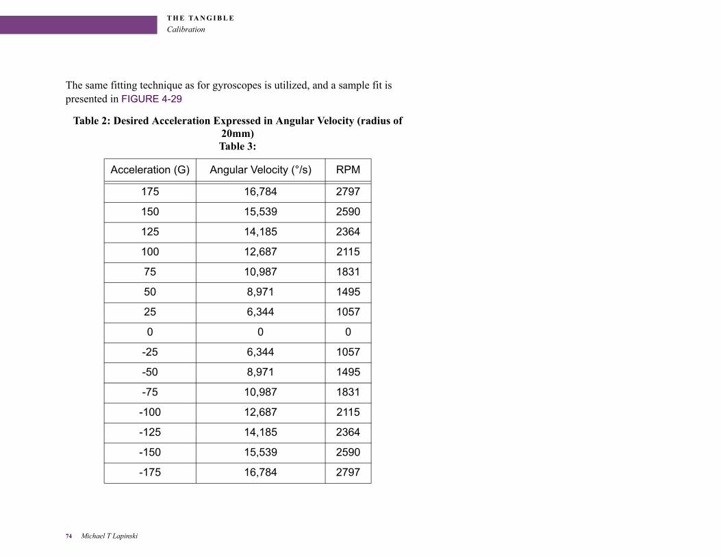
T H E TA N G I B L E
Calibration
The same fitting technique as for gyroscopes is utilized, and a sample fit is presented in FIGURE 4-29
Table 2: Desired Acceleration Expressed in Angular Velocity (radius of 20mm)Table 3:
Acceleration (G) Angular Velocity (°/s) RPM
175 16,784 2797
150 15,539 2590
125 14,185 2364
100 12,687 2115
75 10,987 1831
50 8,971 1495
25 6,344 1057
0 0 0
-25 6,344 1057
-50 8,971 1495
-75 10,987 1831
-100 12,687 2115
-125 14,185 2364
-150 15,539 2590
-175 16,784 2797
74 Michael T Lapinski
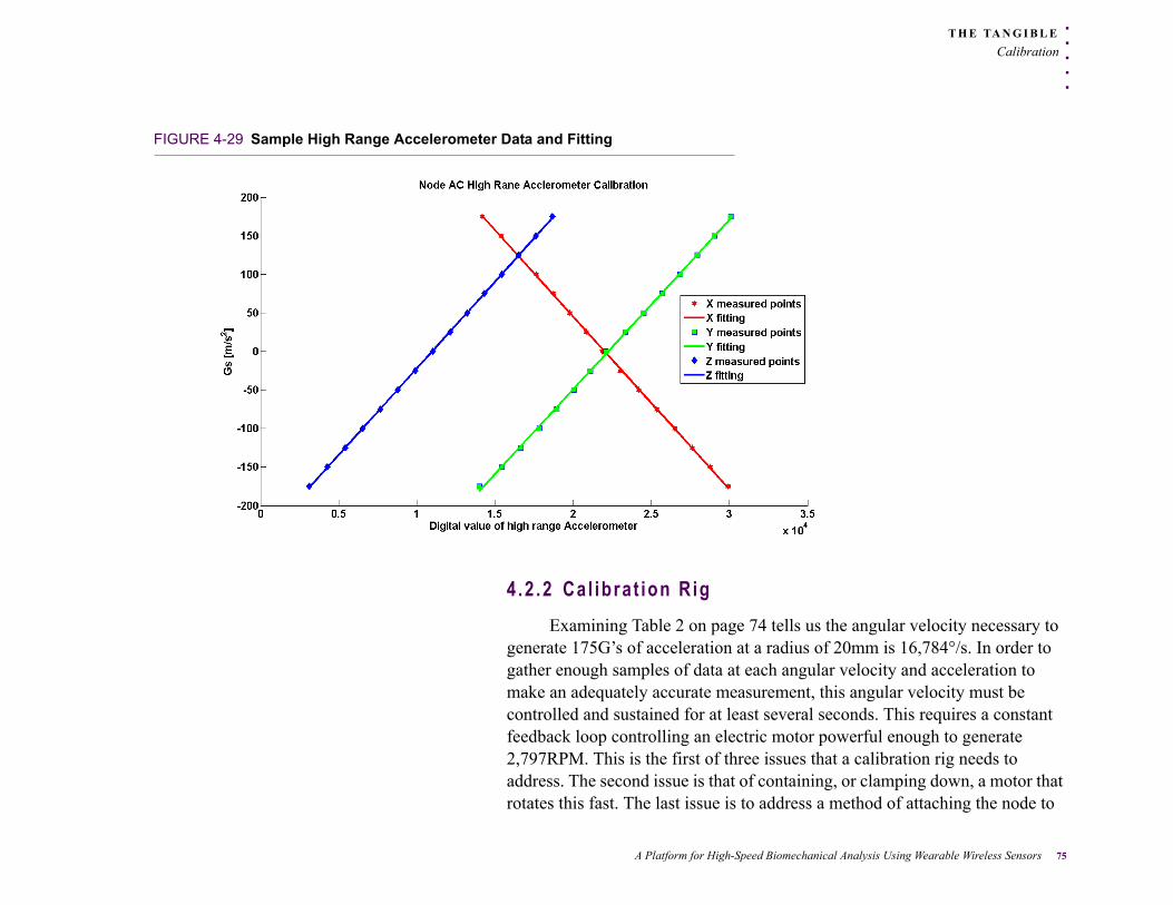
. . .
. .T H E TA N G I B L E
Calibration
FIGURE 4-29 Sample High Range Accelerometer Data and Fitting
4 .2 .2 Ca l ibra t ion Rig
Examining Table 2 on page 74 tells us the angular velocity necessary to generate 175G’s of acceleration at a radius of 20mm is 16,784°/s. In order to gather enough samples of data at each angular velocity and acceleration to make an adequately accurate measurement, this angular velocity must be controlled and sustained for at least several seconds. This requires a constant feedback loop controlling an electric motor powerful enough to generate 2,797RPM. This is the first of three issues that a calibration rig needs to address. The second issue is that of containing, or clamping down, a motor that rotates this fast. The last issue is to address a method of attaching the node to
A Platform for High-Speed Biomechanical Analysis Using Wearable Wireless Sensors 75
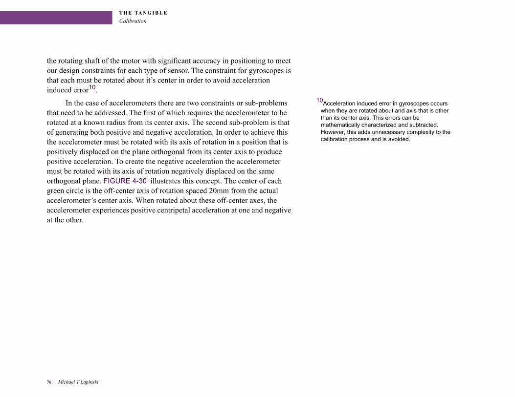
T H E TA N G I B L E
Calibration
the rotating shaft of the motor with significant accuracy in positioning to meet our design constraints for each type of sensor. The constraint for gyroscopes is that each must be rotated about it’s center in order to avoid acceleration induced error10.
10Acceleration induced error in gyroscopes occurs when they are rotated about and axis that is other than its center axis. This errors can be mathematically characterized and subtracted. However, this adds unnecessary complexity to the calibration process and is avoided.
In the case of accelerometers there are two constraints or sub-problems that need to be addressed. The first of which requires the accelerometer to be rotated at a known radius from its center axis. The second sub-problem is that of generating both positive and negative acceleration. In order to achieve this the accelerometer must be rotated with its axis of rotation in a position that is positively displaced on the plane orthogonal from its center axis to produce positive acceleration. To create the negative acceleration the accelerometer must be rotated with its axis of rotation negatively displaced on the same orthogonal plane. FIGURE 4-30 illustrates this concept. The center of each green circle is the off-center axis of rotation spaced 20mm from the actual accelerometer’s center axis. When rotated about these off-center axes, the accelerometer experiences positive centripetal acceleration at one and negative at the other.
76 Michael T Lapinski
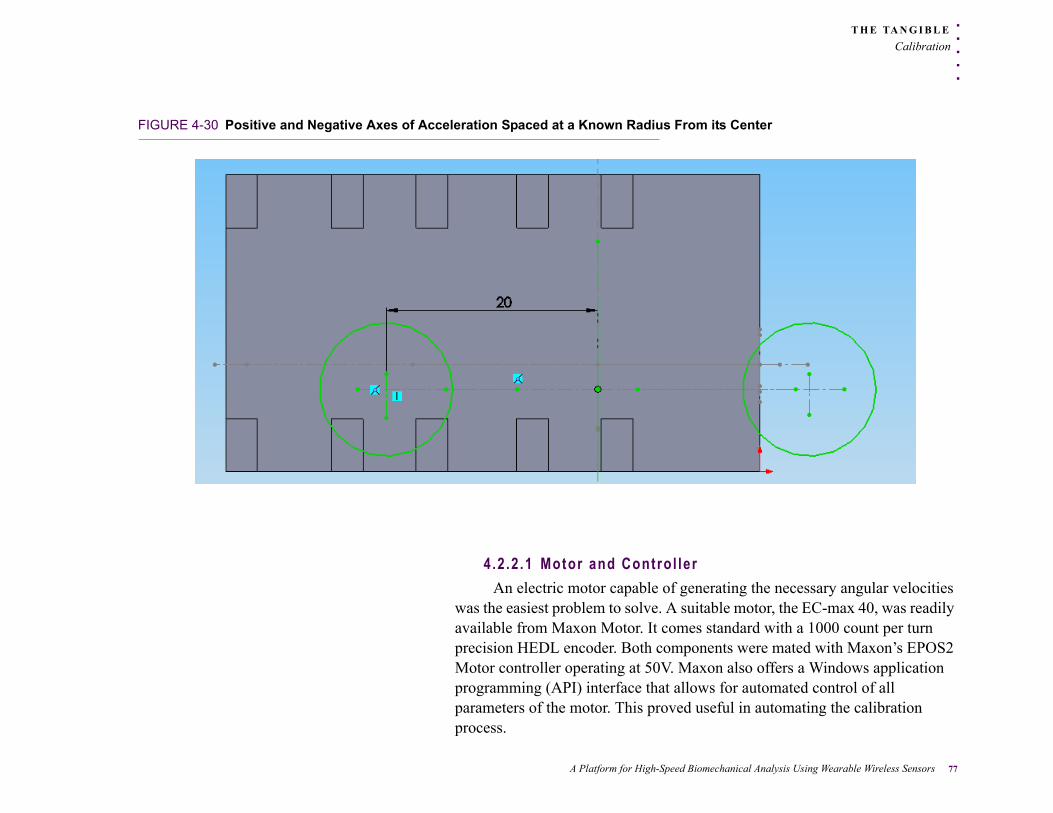
. . .
. .T H E TA N G I B L E
Calibration
FIGURE 4-30 Positive and Negative Axes of Acceleration Spaced at a Known Radius From its Center
4 .2 .2 .1 Motor and Contro l ler
An electric motor capable of generating the necessary angular velocities was the easiest problem to solve. A suitable motor, the EC-max 40, was readily available from Maxon Motor. It comes standard with a 1000 count per turn precision HEDL encoder. Both components were mated with Maxon’s EPOS2 Motor controller operating at 50V. Maxon also offers a Windows application programming (API) interface that allows for automated control of all parameters of the motor. This proved useful in automating the calibration process.
A Platform for High-Speed Biomechanical Analysis Using Wearable Wireless Sensors 77
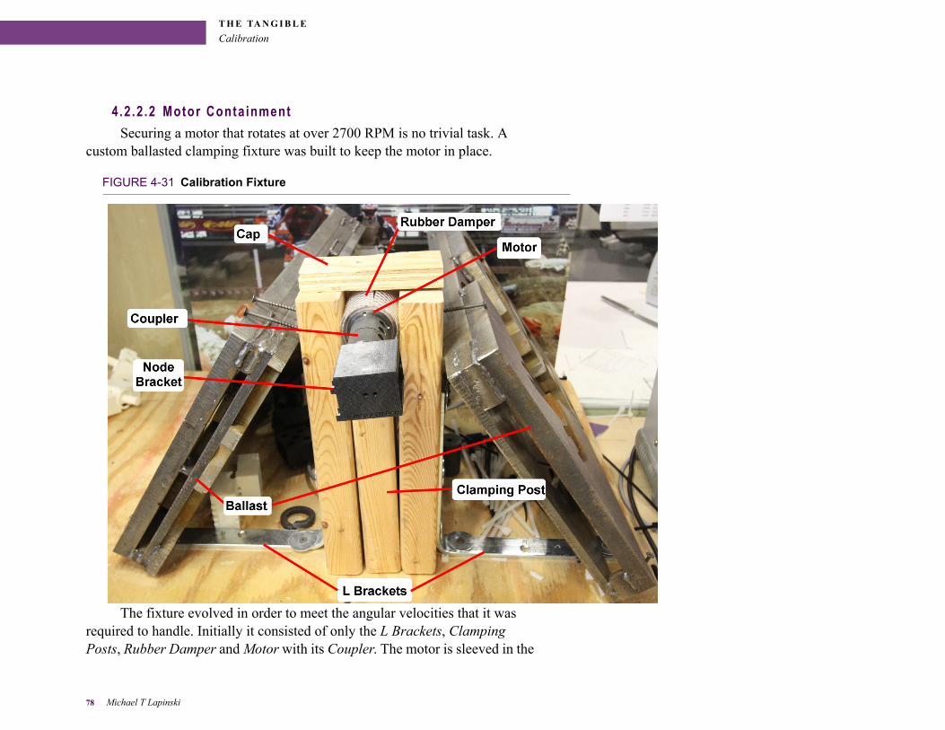
T H E TA N G I B L E
Calibration
4.2 .2 .2 Motor Conta inment
Securing a motor that rotates at over 2700 RPM is no trivial task. A custom ballasted clamping fixture was built to keep the motor in place.
FIGURE 4-31 Calibration Fixture
The fixture evolved in order to meet the angular velocities that it was required to handle. Initially it consisted of only the L Brackets, Clamping Posts, Rubber Damper and Motor with its Coupler. The motor is sleeved in the
78 Michael T Lapinski
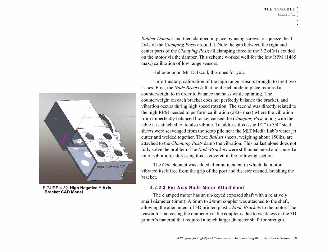
. . .
. .T H E TA N G I B L E
Calibration
Rubber Damper and then clamped in place by using screws to squeeze the 3 2x4s of the Clamping Posts around it. Note the gap between the right and center parts of the Clamping Post; all clamping force of the 3 2x4’s is exuded on the motor via the damper. This scheme worked well for the low RPM (1465 max.) calibration of low range sensors.
Helloooooooo Mr. Dr1scoll, this ones for you.
Unfortunately, calibration of the high range sensors brought to light two issues. First, the Node Brackets that hold each node in place required a counterweight to in order to balance the mass while spinning. The counterweight on each bracket does not perfectly balance the bracket, and vibration occurs during high speed rotation. The second was directly related to the high RPM needed to perform calibration (2833 max) where the vibration from imperfectly balanced bracket caused the Clamping Post, along with the table it is attached to, to also vibrate. To address this issue 1/2” to 3/4” steel sheets were scavenged from the scrap pile near the MIT Media Lab’s water jet cutter and welded together. These Ballast sheets, weighing about 150lbs, are attached to the Clamping Posts damp the vibration. This ballast alone does not fully solve the problem. The Node Brackets were still unbalanced and caused a lot of vibration, addressing this is covered in the following section.
The Cap element was added after an incident in which the motor vibrated itself free from the grip of the post and disaster ensued, breaking the bracket.
FIGURE 4-32 High Negative Y Axis Bracket CAD Model
4 .2 .2 .3 Per Axis Node Motor At tachment
The clamped motor has an un-keyed exposed shaft with a relatively small diameter (6mm). A 6mm to 24mm coupler was attached to the shaft, allowing the attachment of 3D printed plastic Node Brackets to the motor. The reason for increasing the diameter via the coupler is due to weakness in the 3D printer’s material that required a much larger diameter shaft for strength.
A Platform for High-Speed Biomechanical Analysis Using Wearable Wireless Sensors 79
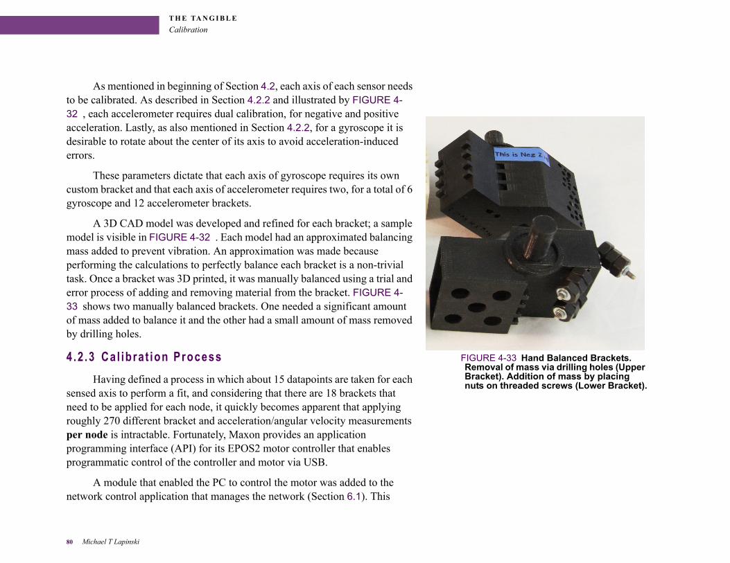
T H E TA N G I B L E
Calibration
As mentioned in beginning of Section 4.2, each axis of each sensor needs to be calibrated. As described in Section 4.2.2 and illustrated by FIGURE 4-32 , each accelerometer requires dual calibration, for negative and positive acceleration. Lastly, as also mentioned in Section 4.2.2, for a gyroscope it is desirable to rotate about the center of its axis to avoid acceleration-induced errors.
These parameters dictate that each axis of gyroscope requires its own custom bracket and that each axis of accelerometer requires two, for a total of 6 gyroscope and 12 accelerometer brackets.
A 3D CAD model was developed and refined for each bracket; a sample model is visible in FIGURE 4-32 . Each model had an approximated balancing mass added to prevent vibration. An approximation was made because performing the calculations to perfectly balance each bracket is a non-trivial task. Once a bracket was 3D printed, it was manually balanced using a trial and error process of adding and removing material from the bracket. FIGURE 4-33 shows two manually balanced brackets. One needed a significant amount of mass added to balance it and the other had a small amount of mass removed by drilling holes.
FIGURE 4-33 Hand Balanced Brackets. Removal of mass via drilling holes (Upper Bracket). Addition of mass by placing nuts on threaded screws (Lower Bracket).
4 .2 .3 Ca l ibra t ion Process
Having defined a process in which about 15 datapoints are taken for each sensed axis to perform a fit, and considering that there are 18 brackets that need to be applied for each node, it quickly becomes apparent that applying roughly 270 different bracket and acceleration/angular velocity measurements per node is intractable. Fortunately, Maxon provides an application programming interface (API) for its EPOS2 motor controller that enables programmatic control of the controller and motor via USB.
A module that enabled the PC to control the motor was added to the network control application that manages the network (Section 6.1). This
80 Michael T Lapinski
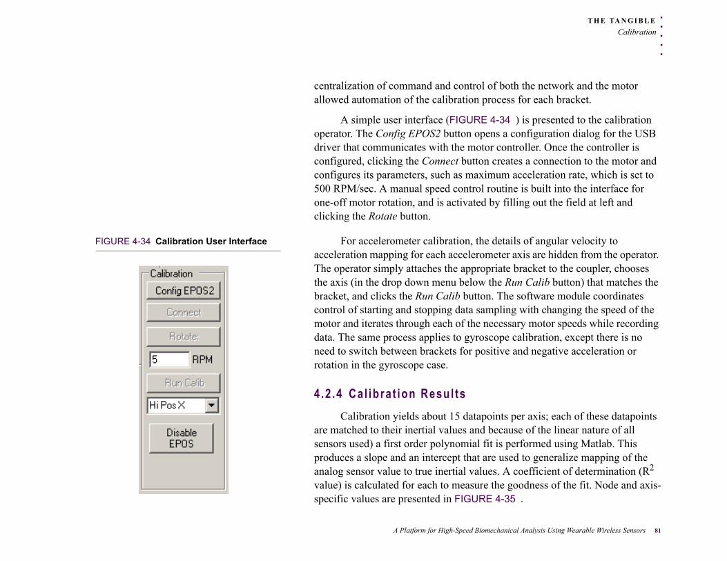
. . .
. .T H E TA N G I B L E
Calibration
centralization of command and control of both the network and the motor allowed automation of the calibration process for each bracket.
A simple user interface (FIGURE 4-34 ) is presented to the calibration operator. The Config EPOS2 button opens a configuration dialog for the USB driver that communicates with the motor controller. Once the controller is configured, clicking the Connect button creates a connection to the motor and configures its parameters, such as maximum acceleration rate, which is set to 500 RPM/sec. A manual speed control routine is built into the interface for one-off motor rotation, and is activated by filling out the field at left and clicking the Rotate button.
FIGURE 4-34 Calibration User Interface For accelerometer calibration, the details of angular velocity to acceleration mapping for each accelerometer axis are hidden from the operator. The operator simply attaches the appropriate bracket to the coupler, chooses the axis (in the drop down menu below the Run Calib button) that matches the bracket, and clicks the Run Calib button. The software module coordinates control of starting and stopping data sampling with changing the speed of the motor and iterates through each of the necessary motor speeds while recording data. The same process applies to gyroscope calibration, except there is no need to switch between brackets for positive and negative acceleration or rotation in the gyroscope case.
4 .2 .4 Ca l ibra t ion Resul ts
Calibration yields about 15 datapoints per axis; each of these datapoints are matched to their inertial values and because of the linear nature of all sensors used) a first order polynomial fit is performed using Matlab. This produces a slope and an intercept that are used to generalize mapping of the analog sensor value to true inertial values. A coefficient of determination (R2 value) is calculated for each to measure the goodness of the fit. Node and axis-specific values are presented in FIGURE 4-35 .
A Platform for High-Speed Biomechanical Analysis Using Wearable Wireless Sensors 81
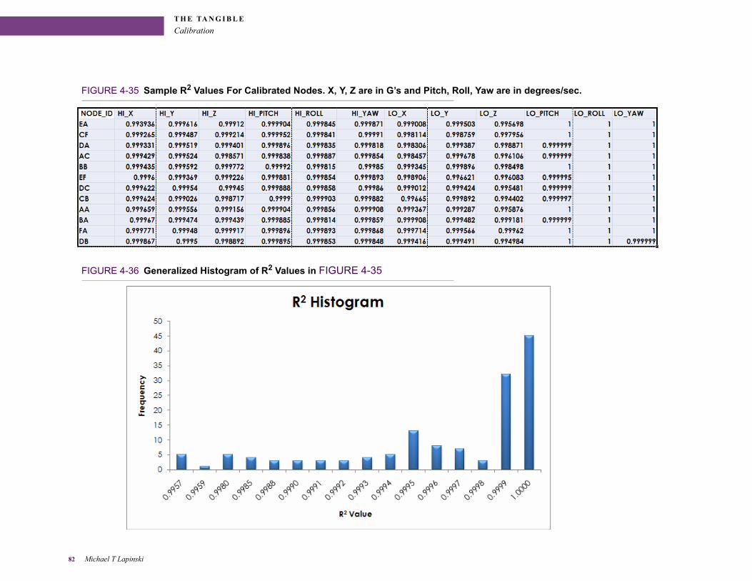
T H E TA N G I B L E
Calibration
FIGURE 4-35 Sample R2 Values For Calibrated Nodes. X, Y, Z are in G’s and Pitch, Roll, Yaw are in degrees/sec.
FIGURE 4-36 Generalized Histogram of R2 Values in FIGURE 4-35
82 Michael T Lapinski
. . .
. .T H E TA N G I B L E
Network Control Basestation
The fit for the low range gyroscope is 1.0 for nearly all nodes and overall the minimum coefficient of determination is 0.993936. This minimum is still a very good fit and indicates that the calibration excellently maps from analog to inertial values and that the output of each sensor is near linear. The histogram in FIGURE 4-36 shows this. A detailed analysis and quantification of the error introduced during calibration is presented in Section 8.1.1.
. . . . . . . . . . . . . . . . . . . . . . . . . . . . . . . . . . . . . . . . . . . . . . . . . . . . . . . . . . .4 . 3 N E T W O R K C O N T R O L B A S E S T A T I O N
Although the RF protocol has been entirely re-designed, the basestation is the only piece of hardware that is reused from the Sensemble project and a high level summary will be presented here. A detailed description is available in Ryan Aylwards Masters Thesis [74] and the author’s Masters Thesis [7]. It is important to note that only the hardware has been reused. The firmware and client side code that controls the basestation are all specific to the new node hardware and athletic activity.
The basestation has essentially 2 pieces of hardware, a limited capability microcontroller that can act a a USB slave and a wireless transceiver. The wireless transceiver is the same Nordic nRF2401[76] that is used in the node. The microcontroller is a Silicon Labs C8051F320 [77] running at 24MHz. It reads commands via a USB connection to a host PC, interprets them and instructs the nRF2401 to transmit the data wirelessly to the network of nodes via a Serial Peripheral Interface.
A Platform for High-Speed Biomechanical Analysis Using Wearable Wireless Sensors 83
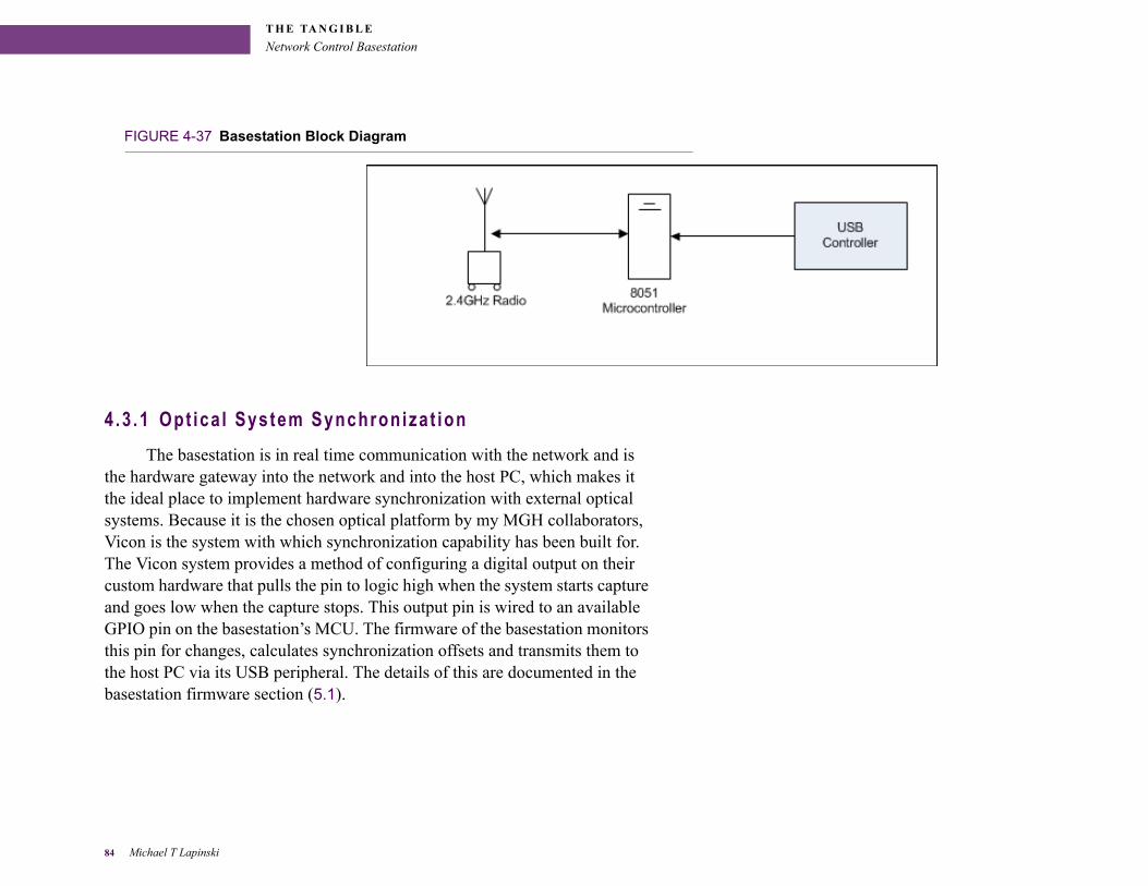
T H E TA N G I B L E
Network Control Basestation
FIGURE 4-37 Basestation Block Diagram
4.3 .1 Opt ica l System Synchronizat ion
The basestation is in real time communication with the network and is the hardware gateway into the network and into the host PC, which makes it the ideal place to implement hardware synchronization with external optical systems. Because it is the chosen optical platform by my MGH collaborators, Vicon is the system with which synchronization capability has been built for. The Vicon system provides a method of configuring a digital output on their custom hardware that pulls the pin to logic high when the system starts capture and goes low when the capture stops. This output pin is wired to an available GPIO pin on the basestation’s MCU. The firmware of the basestation monitors this pin for changes, calculates synchronization offsets and transmits them to the host PC via its USB peripheral. The details of this are documented in the basestation firmware section (5.1).
84 Michael T Lapinski
. . .
. .T H E TA N G I B L E
Data Translator
. . . . . . . . . . . . . . . . . . . . . . . . . . . . . . . . . . . . . . . . . . . . . . . . . . . . . . . . . . .4 . 4 D A T A T R A N S L A T O R
As briefly described in 3.2.2, a custom data retrieval interface needed to be implemented in order to read data from the µSD, because it is written to the card as raw sectors, not a standard filesystem. Instead of building a custom piece of hardware, the Atmel EVK1101 [78] development board was leveraged. The EVK1101 is an all-in-one platform for developing test applications for the Atmel UC3B0256 microcontroller, the same microcontroller used in hardware revision 2 of the wireless inertial node. Having the development environment and familiarity with the board made it a natural choice. Other than a µSD to SD adapter, no hardware modifications were made to the board and it was used as-is.
A Platform for High-Speed Biomechanical Analysis Using Wearable Wireless Sensors 85

T H E TA N G I B L E
Data Translator
86 Michael T Lapinski
. . .
. .T H E I N T A N G I B L E
. . . .
. . . . . . . . . . . . . . . . . . . . . . . . . . . . . . . . . . . . . .THE INTANGIBLE
The intangible is something that cannot be seen or touched. Here it consists of the firmware that operates the tangibles. The operating principals of three hardware devices are described, starting with the basestation, then the inertial node(s) and lastly, the data translator, in order to better understand how the system functions as a whole.
A Platform for High-Speed Biomechanical Analysis Using Wearable Wireless Sensors 87
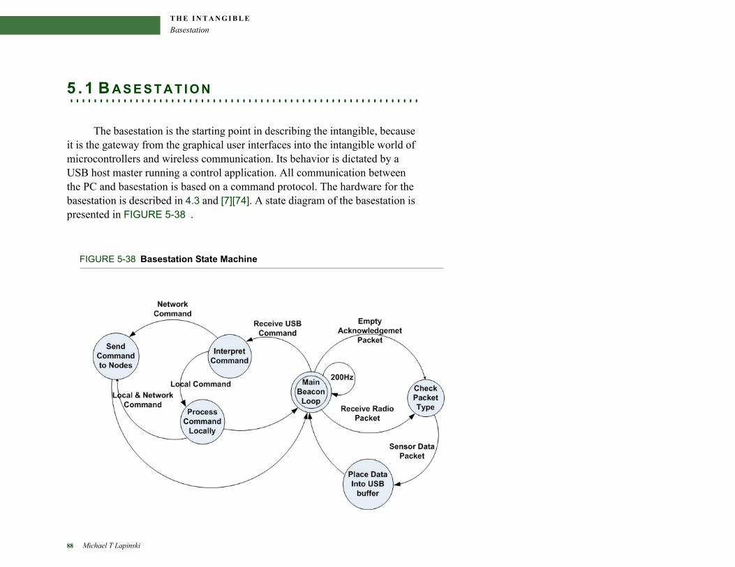
T H E I N T A N G I B L E
Basestation
. . . . . . . . . . . . . . . . . . . . . . . . . . . . . . . . . . . . . . . . . . . . . . . . . . . . . . . . . . .5 . 1 B A S E S T A T I O N
The basestation is the starting point in describing the intangible, because it is the gateway from the graphical user interfaces into the intangible world of microcontrollers and wireless communication. Its behavior is dictated by a USB host master running a control application. All communication between the PC and basestation is based on a command protocol. The hardware for the basestation is described in 4.3 and [7][74]. A state diagram of the basestation is presented in FIGURE 5-38 .
FIGURE 5-38 Basestation State Machine
88 Michael T Lapinski
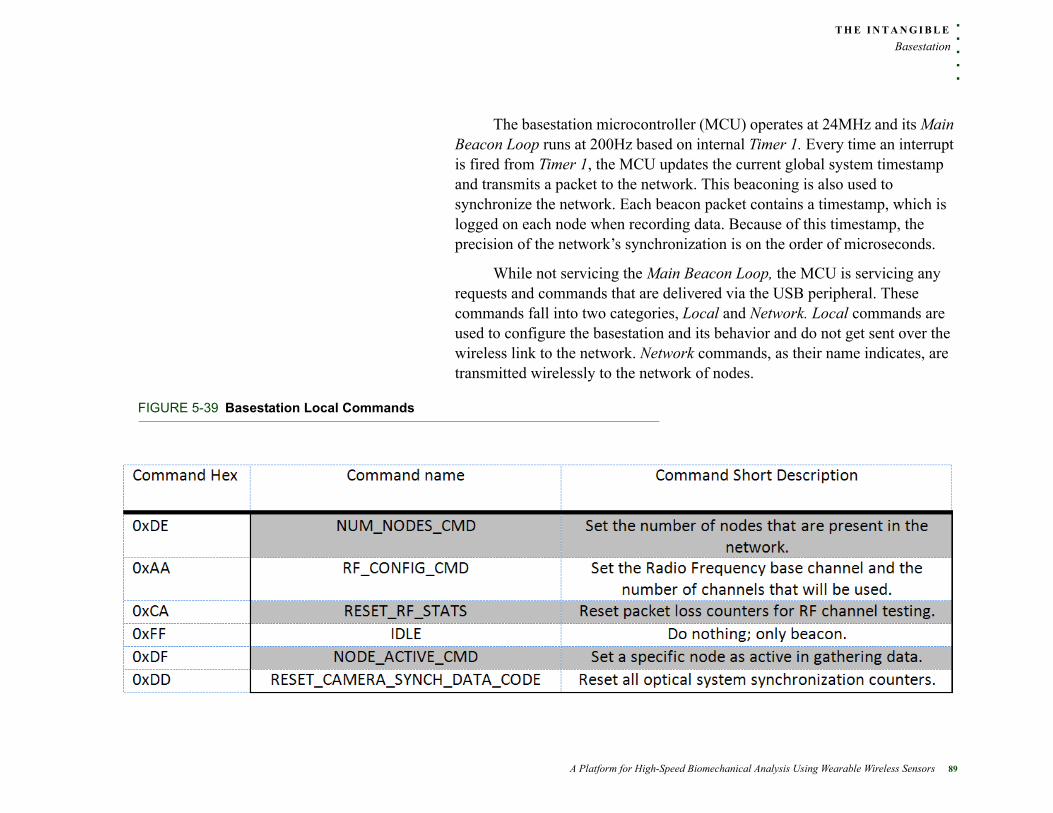
. . .
. .T H E I N T A N G I B L E
Basestation
The basestation microcontroller (MCU) operates at 24MHz and its Main Beacon Loop runs at 200Hz based on internal Timer 1. Every time an interrupt is fired from Timer 1, the MCU updates the current global system timestamp and transmits a packet to the network. This beaconing is also used to synchronize the network. Each beacon packet contains a timestamp, which is logged on each node when recording data. Because of this timestamp, the precision of the network’s synchronization is on the order of microseconds.
While not servicing the Main Beacon Loop, the MCU is servicing any requests and commands that are delivered via the USB peripheral. These commands fall into two categories, Local and Network. Local commands are used to configure the basestation and its behavior and do not get sent over the wireless link to the network. Network commands, as their name indicates, are transmitted wirelessly to the network of nodes.
FIGURE 5-39 Basestation Local Commands
A Platform for High-Speed Biomechanical Analysis Using Wearable Wireless Sensors 89
T H E I N T A N G I B L E
Basestation
Local commands are presented in FIGURE 5-39 and Network commands are presented in FIGURE 5-40 . The mechanism for the basestation to communicate back to the host PC is a USB Buffer that is filled and transmitted to the host PC via the MCU’s USB peripheral.
The NUM_NODES_CMD informs the basestation as to how many nodes will be operating in the network. It is complemented by the NODE_ACTIVE_CMD command, which specifies whether a specific active node is gathering data. This is a crucial mechanism for allowing the network to continue operation even with a node that maybe misbehaving and not able to gather data.
The IDLE command instructs the basestation to do nothing. The commands RF_CONFIG_CMD and RESET_RF_STATS are used to configure the communication frequencies used and reset counters and parameters related to testing the RF environment quality. The RESET_CAMERA_SYNCH_DATA_CODE, is covered in the optical system synchronization sections 5.1.1, 6.1.8 and 7.4.
90 Michael T Lapinski
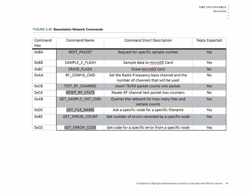
. . .
. .T H E I N T A N G I B L E
Basestation
FIGURE 5-40 Basestation Network Commands
A Platform for High-Speed Biomechanical Analysis Using Wearable Wireless Sensors 91
T H E I N T A N G I B L E
Basestation
Network commands have the additional property of determining whether or not a reply is expected from the node once it has received and processed the packet. A reply is not expected from all commands except the RF_CONFIG_CMD command. This is because, if the network is reconfigured to a different frequency, the node will be broadcasting on the new frequency, which the basestation is not yet utilizing. Further, the RF_CONFIG_CMD is considered to be a Local and Network command because both the basestation and nodes must process it. The TEST_RF_CHANNEL command adds additional data to all packets that allow for calculating packet loss metrics for the network. The RESET_RF_STATS command resets received/transmitted packet counters on the node. These counters are used to measure the RF channel quality.
The NEXT_PACKET command, whose purpose was to send a specific data sample wirelessly, has been deprecated because the packet length can no longer handle all of the sampled sensor data. The expected reply packet contained the analog sensor data from a given sample number, and when this data was received it was placed into the USB Buffer and transmitted to the host PC.
The SAMPLE_2_FLASH command instructs the network to begin sampling data. The basestation continues to beacon this command until interrupted via USB by the host PC or until it has received a packet indicating from every node in the network that it finished its sampling loop. Which nodes are expected to reply is based on previous NUM_NODES_CMD and NODE_ACTIVE_CMD commands.
The ERASE_FLASH command instructs each node in the network to erase its µSD card and the MCUs own internal flash, which stores various counters and memory allocation information for previously sampled data. A reply is expected from each node when the data has been erased. Again, which
92 Michael T Lapinski
. . .
. .T H E I N T A N G I B L E
Basestation
nodes are expected to reply is based on previous NUM_NODES_CMD and NODE_ACTIVE_CMD commands.
11Please refer to Section 3.1.0.3 for definition of a gesture
The GET_SAMPLE_CNT_CMD requests the number of gestures11 of data that have been recorded by each node and also the number of samples per gesture11.
The GET_FILE_NAME command requests a specific filename from a specific node based on a numerical index. This index is sent by the PC host and inserted into the outgoing packet. The index indicates which name in the list of filenames is to be transmitted back by the node.
A GET_ERROR_COUNT command requests the value of a specific node’s internal error counter - a count of how many errors the node has experienced. It is complemented by the GET_ERROR_CODE command, which is sent to a specific node with a specific error code index. The specified node selects the index error code in its error code list and transmits it back to the basestation.
It is easy to see that the basestation is an arbiter between the host PC and the network of nodes that does some simple bookkeeping to track which nodes are present on the network and how they are expected to behave.
5 .1 .1 Opt ica l System Synchroniza t ion
Section 4.3.1 describes the hardware interface between the wearable network and the Vicon optical capture system in order to synchronize them. The bulk of the synchronization is handled by the basestation firmware and the logic is based on monitoring the Vicon output pin (an input to the basestation) to see if the optical system is recording or not.
The synchronization starts when the basestation receives a SAMPLE_2_FLASH command from the host PC and the Vicon GPIO pin is logic zero. When this command is seen, the basestation starts a counter that
A Platform for High-Speed Biomechanical Analysis Using Wearable Wireless Sensors 93

T H E I N T A N G I B L E
Basestation
measures the number of milliseconds that have elapsed since it was received; the start of this timer indicates the start time of data recording. The only delay that is present is that of transferring the data packet to the nRF2401 and its wireless transmission. This delay is on the order of µseconds and presents negligible error into the synchronization. Once the Vicon GPIO pin changes state to logic high, indicating the optical system has start recording, the counter is stopped and read. This reading yields Δ-Start, which represents the amount of time that the wearable inertial system was recording before the optical system started. In order to synchronize the two systems, Δ-Start milliseconds of data must be pruned from the start of any inertial data stream.
FIGURE 5-41 Optical Synchronization Timing Diagram
94 Michael T Lapinski
. . .
. .T H E I N T A N G I B L E
Node Startup
. . . . . . . . . . . . . . . . . . . . . . . . . . . . . . . . . . . . . . . . . . . . . . . . . . . . . . . . . . .5 . 2 N O D E S T A R T U P
The Atmel AVR32 UC3A3256 [79] microcontroller (MCU) is the focal point of each wearable node, a block diagram of which is depicted in FIGURE 5-42 . At startup its flash memory is checked and initialized, if necessary, and the error handling subsystem is initialized. After this, all clocks are initialized and configured. With properly configured clocks, all communication peripherals can be configured and tested. Once communication buses have been made available, each connected hardware device can be configured for operation and queried to ensure it is operating properly. Once all hardware components and subsystems have been confirmed to be properly working, the node begins servicing interrupts and processing command data packets from the wireless transceiver.
A Platform for High-Speed Biomechanical Analysis Using Wearable Wireless Sensors 95
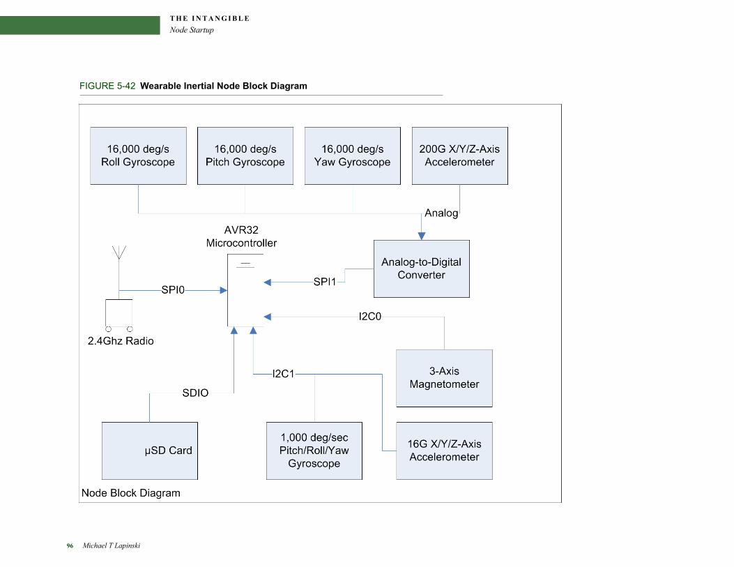
T H E I N T A N G I B L E
Node Startup
FIGURE 5-42 Wearable Inertial Node Block Diagram
96 Michael T Lapinski
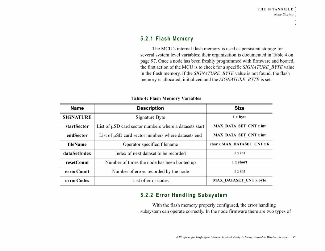
. . .
. .T H E I N T A N G I B L E
Node Startup
5 .2 .1 F lash Memory
The MCU’s internal flash memory is used as persistent storage for several system level variables; their organization is documented in Table 4 on page 97. Once a node has been freshly programmed with firmware and booted, the first action of the MCU is to check for a specific SIGNATURE_BYTE value in the flash memory. If the SIGNATURE_BYTE value is not found, the flash memory is allocated, initialized and the SIGNATURE_BYTE is set.
Table 4: Flash Memory Variables
Name Description Size
SIGNATURE Signature Byte 1 x byte
startSector List of µSD card sector numbers where a datasets start MAX_DATA_SET_CNT x int
endSector List of µSD card sector numbers where datasets end MAX_DATA_SET_CNT x int
fileName Operator specified filename char x MAX_DATASET_CNT x 6
dataSetIndex Index of next dataset to be recorded 1 x int
resetCount Number of times the node has been booted up 1 x short
errorCount Number of errors recorded by the node 1 x int
errorCodes List of error codes MAX_DATASET_CNT x byte
5 .2 .2 Error Handl ing Subsystem
With the flash memory properly configured, the error handling subsystem can operate correctly. In the node firmware there are two types of
A Platform for High-Speed Biomechanical Analysis Using Wearable Wireless Sensors 97
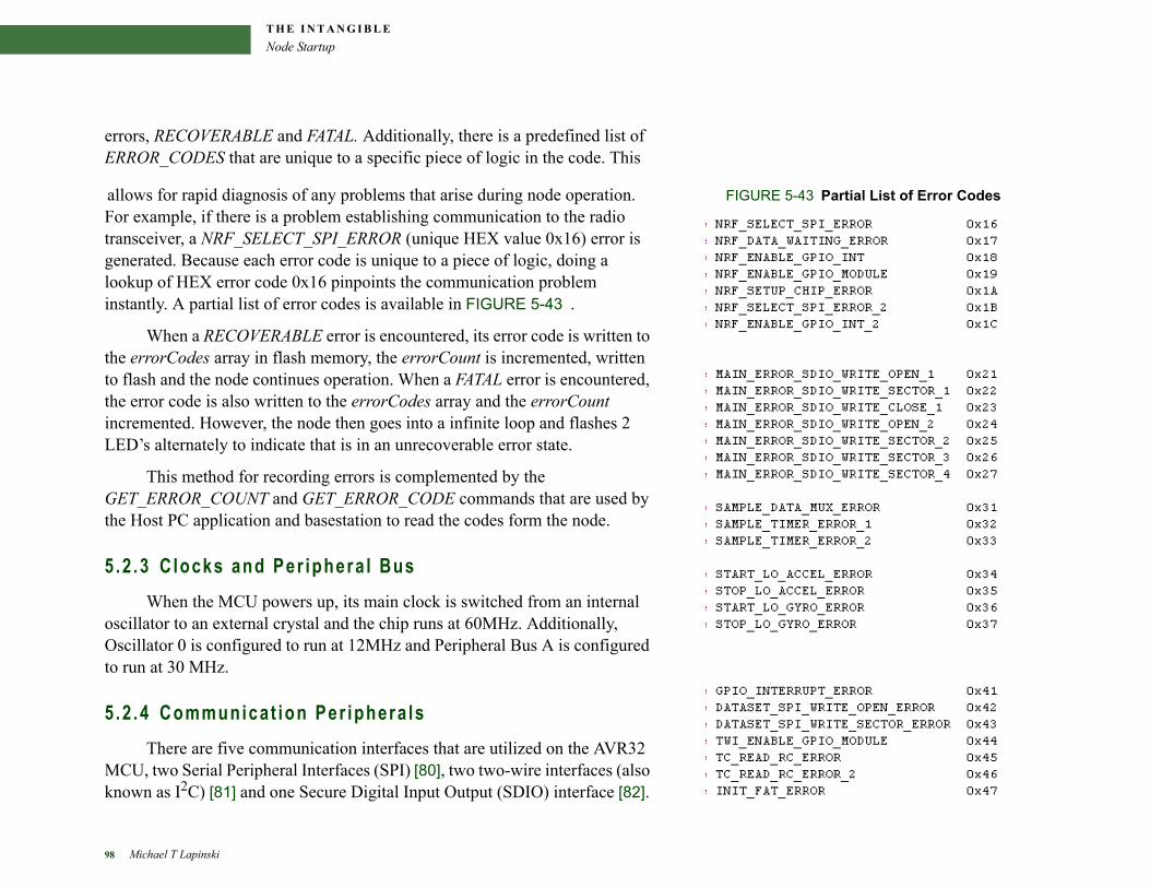
T H E I N T A N G I B L E
Node Startup
errors, RECOVERABLE and FATAL. Additionally, there is a predefined list of ERROR_CODES that are unique to a specific piece of logic in the code. This
FIGURE 5-43 Partial List of Error Codesallows for rapid diagnosis of any problems that arise during node operation. For example, if there is a problem establishing communication to the radio transceiver, a NRF_SELECT_SPI_ERROR (unique HEX value 0x16) error is generated. Because each error code is unique to a piece of logic, doing a lookup of HEX error code 0x16 pinpoints the communication problem instantly. A partial list of error codes is available in FIGURE 5-43 .
When a RECOVERABLE error is encountered, its error code is written to the errorCodes array in flash memory, the errorCount is incremented, written to flash and the node continues operation. When a FATAL error is encountered, the error code is also written to the errorCodes array and the errorCount incremented. However, the node then goes into a infinite loop and flashes 2 LED’s alternately to indicate that is in an unrecoverable error state.
This method for recording errors is complemented by the GET_ERROR_COUNT and GET_ERROR_CODE commands that are used by the Host PC application and basestation to read the codes form the node.
5 .2 .3 C locks and Per iphera l Bus
When the MCU powers up, its main clock is switched from an internal oscillator to an external crystal and the chip runs at 60MHz. Additionally, Oscillator 0 is configured to run at 12MHz and Peripheral Bus A is configured to run at 30 MHz.
5 .2 .4 Communicat ion Per iphera ls
There are five communication interfaces that are utilized on the AVR32 MCU, two Serial Peripheral Interfaces (SPI) [80], two two-wire interfaces (also known as I2C) [81] and one Secure Digital Input Output (SDIO) interface [82].
98 Michael T Lapinski
. . .
. .T H E I N T A N G I B L E
Node Startup
All three are bus interfaces supporting multiple devices, however in this implementation the bus feature is not used for all interfaces. In all cases the MCU is the master, while the connected devices are slaved.
The zeroth SPI bus (SPI0) is used to communicate with the radio transceiver. It is clocked at 4MHz and is exclusively used by the radio to allow for servicing of incoming radio packets at any time. One clock pin and two data lines (one input and one output) are utilized for communication. A chip select pin is also dedicated to each specific device on the bus. In this case, there is a chip select pin wired to the transceiver.
The first SPI bus (SPI1) is used to communicate with the analog-to-digital converter. Is it also clocked at 4MHz and exclusively dedicated to the analog-to-digital converter because no other SPI devices exist in the system. As with SPI0, one clock pin and two data lines are used for communication.
The one and only SDIO bus has one µSD card slot wired to it, and, because it is a high speed interface, it operates at 30MHz. The node design exploits the parallel mode of operating the SDIO interface and has a command pin, clock pin and four data pins dedicated to it.
I2C bus zero is dedicated to the on-board magnetometer and operates at a clock speed of 400 kHz for communication. As the two-wire interface name suggests, there are two pins dedicated to an I2C device, one as a clock and one for data.
I2C bus one makes use of the multi-device bus feature and communicates with the low- range gyroscope and the low-range accelerometer. Each of these devices is also clocked at 400 kHz. Again, two pins are dedicated to I2C1, one for clocking and one for data.
A Platform for High-Speed Biomechanical Analysis Using Wearable Wireless Sensors 99
T H E I N T A N G I B L E
Node Startup
5 .2 .5 Hardware Dev ices
Once all communication peripherals are have been initialized without error, individual device configuration can occur.
5.2 .5 .1 µSD Card
The µSD card is connected via the SDIO bus. In previous versions of the node hardware, SPI-based communication was used to read and write from the SD card and its serial nature created a bottleneck in the system while writing sampled data to the card. One of the motivations for choosing the UC3A3 MCU was that it features a dedicated and parallel, therefore much faster, SDIO bus. Along with the hardware peripheral, Atmel provided a software framework [82] and a library for programmers and took the complicated process of implementing the SDIO Specification[83] upon themselves. Once the SDIO peripheral has been configured, the programmer calls a single function to negotiate and establish communication with the card. After this, the card can be opened/closed and sectors can be written and deleted.
5.2 .5 .2 High Range Gyroscopes
The ADXRS649 [84] high range gyroscope has an analog output and does not communicate directly with the MCU, hence it does not have any software-based configuration. However each gyroscope uses external filtering capacitors to limit its output bandwidth to 500Hz, to avoid aliasing. The output of the three onboard ADXRS649 gyroscopes is sampled by the Analog Devices AD7606 [85] analog-to-digital converter and transmitted to the MCU via SPI1.
5.2 .5 .3 High Range Accelerometer
As with the high range gyroscopes, the Analog Devices ADXL377 [88] high range accelerometer only has analog outputs, which are sampled by the analog-to-digital converter. It is also bandwidth limited by external filtering
100 Michael T Lapinski
. . .
. .T H E I N T A N G I B L E
Node Startup
capacitors, which are matched to chip-internal resistors for anti-aliasing to 500Hz.
5.2 .5 .4 Analog- to-Dig i ta l Converter
The Analog Devices AD7606 16-bit analog-to-digital (A2D) converter is connected to the MCU via SPI1. It has no other software based configuration, and all of its functionality and communication is based on GPIO pins that are wired from the A2D to the MCU. The SPI1 bus is used only to transmit six 16-bit analog-to-digital conversion values to the MCU. The GPIO pins that are used are as follows:
1 CONV_CTRL - wired to the chip’s CONVST A and CONVST B pins.
The MCU drives this pin and a transition from logic 0 to logic 1 starts
the analog-to-digital conversion process.
2 A2D_BUSY - while the conversion is active, this pin is held in logic 1,
and when finished the A2D transitions the pin to logic 0. The MCU
internally polls this pin to determine when conversion data is
available.
3 A2D_RESET - The MCU can pull this pin low to reset the A2D.
Specific configuration parameters are configured using external pins present on the AD7606 chip itself. Other than power and ground pin connections, there are three other pins that control the A2D’s behavior. They are:
1 Communication Interface - the PAR/SER/BYTE SEL pin is pulled up to
logic 1. The puts the chip in SPI communication mode.
2 Standby - the STDBY pin is pulled up to logic 1, keeping the chip out of
standby mode at all times.
3 Reference Voltage Selection - set to logic 0, allowing the A2D to use its
own internally-generated reference voltage.
A Platform for High-Speed Biomechanical Analysis Using Wearable Wireless Sensors 101
T H E I N T A N G I B L E
Node Startup
5.2 .5 .5 Low Range Gyroscope12except for a pin that is pulled down to specify I2C
addressThe Invensense IMU-3000 [87] 3-axis gyroscope is the first part we
discuss that is exclusively12 controlled and configured via software and does not require any external parts to configure its sensing capability. The process for configuring the IMU-3000, is by setting specific values in registers that are stored in its own EEPROM. As a sanity check after each register is written to the IMU-3000 it is then read back and compared to the expected value. If there is an inconsistency, a FATAL error code is generated.
The target sampling rate for the IMU-3000 is its maximum rate of 5Hz and its desired range is ±1,000°/second. Because of this, the register that controls its low pass filters and scale (0x16) is set to 0x10, which yields a 256Hz low pass filter and ±1,000°/second range.
When the low pass filter register is configured for the IMU-3000 internally to cutoff at 256Hz, the internal analog gyroscopes are sampled at 8kHz. This sampling rate must be scaled down via a sample rate register to match the desired sample rate of 500Hz. This is achieved by writing a value of 0x0F to the appropriate register (0x19).
Now that the behavior of the IMU-3000 has been configured, the interrupt it generates for the MCU to inform it when gyroscope data is ready is configured. The interrupt is physically enabled by wiring the IMU-3000’s AD0 pin to a GPIO pin on the MCU. Additionally, the IMU-3000 is configured to generate an interrupt when data is ready and clear the interrupt when any register is read by setting a value of 0x31 to register 0x17.
5.2 .5 .6 Low Range Accelerometer
Similarly to the low rage gyroscope, the Analog Devices ADXL345 [88] low range accelerometer is also fully configured using a software interface12, and has an interrupt pin wired to the MCU to inform it when data is available. It also has a set of registers that are written to configure its operation.
102 Michael T Lapinski
. . .
. .T H E I N T A N G I B L E
Node Startup
As with the IMU-3000, the desired sampling rate for the ADXL345 is 500Hz, however the chip only supports 400Hz and 800Hz sampling. The 800Hz option was chosen to maximize the amount of data available. This required setting the bandwidth rate register (0x2C) to 0x0D.
The interrupt map register (0x2F) is configured to transition the ADXL345’s INT1 pin from logic 0 to logic 1 when data is available by setting its value to 0x7F. The interrupts are enabled by setting a separate register (0x2E) to 0x80.
5.2 .5 .7 Magnetometer
The Honeywell HMC5843 [89] magnetometer is configured via software in the same EEPROM register-writing manner as the low range gyroscope and accelerometer. Two registers need to be written to configure the magnetometer as desired. The sampling rate is set to the maximum of 50Hz by writing 0x18 to Configuration Register A (0x00). The device is started and set to continuous-conversion mode by writing 0x00 to the mode register (0x02).
5.2 .5 .8 RF Transceiver
In addition to communicating on SPI0, the Nordic NRF2401 [76] has three additional pins that are wired to the MCU for proper radio operation. These are a chip enable pin (CE), a power up pin (PWR_UP) and a data ready pin (DR). The CE pin is used to toggle the radio between standby and receive/transmit modes. The PWR_UP pin is used to turn the radio on and off. The DR pin indicates when the radio has received a full data packet and is ready for the MCU master to read it from the radio. All of these pins are configured in the MCU as general purpose input/output (GPIO). Additionally, a service interrupt is associated with the DR pin transitioning from logic zero to logic one.
A Platform for High-Speed Biomechanical Analysis Using Wearable Wireless Sensors 103
T H E I N T A N G I B L E
Node Operation
With a properly configured SPI bus and associated GPIO pins, the radio is set to standby mode and the configuration data (packet length, network address, operating frequency, datarate) is sent over the SPI bus. Once configured, the transceiver is set to receive mode and the MCU waits for an interrupt on the DR pin.
. . . . . . . . . . . . . . . . . . . . . . . . . . . . . . . . . . . . . . . . . . . . . . . . . . . . . . . . . . .5 . 3 N O D E O P E R A T I O N
Each wearable node is controlled by the Network commands (FIGURE 5-40 ) broadcast by the basestation. An interrupt is fired when the radio receives a valid data packet. The packet is read from the radio by the MCU and decoded to determine what command it contains. Based on the command, the MCU reacts and takes action. The behavior of the node will be documented here for all commands except those that pertain to RF configuration and testing.
5.3 .0 .1 Error Commands
The GET_ERROR_COUNT and GET_ERROR_CODE commands are used together to read errors from the node. When GET_ERROR_COUNT is received by the node, the errorCount (Section 5.2.1) is read from the flash memory, packaged into the next RF packet to be transmitted and sent back to the basestation. A GET_ERROR_CODE command is accompanied by an integer index. This index is used to read the index error code in the errorCodes flash memory array (Section 5.2.1) and copy them into the next outgoing RF packet such that it can be transmitted back to the basestation.
104 Michael T Lapinski
. . .
. .T H E I N T A N G I B L E
Node Operation
5.3 .0 .2 Id le Command
When an IDLE command is received by a node, the global SYSTEM_STATE of the node is set to SYS_IDLE, to indicate that the node is idle, and a packet with no payload is transmitted back to the basestation.
5.3 .0 .3 Next Packet Command
As mentioned in 5.1, the NEXT_PACKET command is deprecated and is no longer tractable to support. When a node receives a command of this type it is treated in the same manner as a SYS_IDLE command.
5.3 .0 .4 Erase F lash Command
The ERASE_FLASH command erases the contents of the MCU’s internal flash that is used for storing data (Section 5.2.1) and also erases the sectors of the µSD card that have sampled data stored on them. After this, all counters used to keep track of sector position on the µSD card and those stored in the MCU’s flash are re-initialized to zero and the SIGNATURE_BYTE is re-written to flash.
5.3 .0 .5 Sample to F lash Command13Typically 8 seconds. The most complicated of all commands is the SAMPLE_2_FLASH
command. When received, the node goes into a data gathering loop and gathers data for a predetermined number13 of seconds at 1000Hz for the high range sensors, 500Hz for the low range sensors and 50Hz for the magnetometer. The global SYSTEM_STATE variable is set to SAMPLING_TO_FLASH.
All data is stored in two RAM buffers that are 512 bytes in size. Which buffer is currently being used to store data is determined by what buffer is currently being written to the µSD card. If a buffer is in the process of being written, new data cannot be added to it, as this would cause inconsistences in the data There are two types of data: magnetometer and inertial. Both types
A Platform for High-Speed Biomechanical Analysis Using Wearable Wireless Sensors 105
T H E I N T A N G I B L E
Node Operation
have a set length of 28 bytes. This is the minimum number of bytes that can be used to store a SAMPLE_NUMBER14, a global timestamp (provided by the basestation in the incoming packet) and the analog inertial sensor data. Rather than deal with the overhead needed to handle variable length data packets, the 10 bytes of magnetometer data are padded to make the data length 28 bytes. A global index into the data buffer is kept, and before any data is stored into a RAM buffer, a check is done to ensure that storing 28 bytes will not exceed the 512 byte length of the buffer. If a store will exceed the 512 length, the current buffer is marked to be stored to the µSD card and the other buffer is utilized.
Each SAMPLE_2_FLASH command packet is accompanied by a 6-byte filename. This filename is written to the first sample section of the current 512-byte data buffer. It is uniquely identified by 4 signature bytes and is called the HEADER_DATA.
14SAMPLE_NUMBER is simply a counter that is initialized to zero when the timer is configured and started. It is incremented by one every time the timer fires.
The entire process is managed by an internal timer that fires once every millisecond. When a SAMPLE_2_FLASH command is received, this timer is started. Each time the timer is fired, a series of decisions and actions are taken based on the current SAMPLE_NUMBER14.
The first check that is performed is to determine weather the magnetometer should be read or not. This is done by taking the modulus of SAMPLE_NUMBER by 20. If the result is zero, the compass’ 50Hz sampling should have data ready, then a Direct Memory Access (DMA) transaction is initiated and started. If the result of the modulus is not zero, a global variable that stores the state of the magnetometer’s DMA transaction is read. If this variable indicates that the transaction has completed, the magnetometer data is copied to the current µSD card buffer. If neither condition is met, no action is taken.
Every time the timer fires, the AD7606 is queried for new high range data from the ADXL377 and the ADXRS649’s. This data is stored into the current RAM buffer. After sampling high range data, the GPIO pins for the
106 Michael T Lapinski

. . .
. .T H E I N T A N G I B L E
Node Operation
ADXL345 and IMU-3000 are checked to determine if data is ready. If data is available from the ADXL345, its data registers are read and the results are stored in the current RAM buffer. Otherwise, NULL values are stored into the current RAM buffer. The same approach is taken with the IMU-3000.
If the current SAMPLE_NUMBER has reached the global maximum number of samples, the timer is stopped and the global SYSTEM_STATE variable is updated to FLASH_FULL. A full dataset has been successfully recorded and relevant data that is stored in flash memory (Section 5.2.1) can be appended and updated. This means that the startSector of the currently completed dataset is appended, as is the endSector and fileName. The dataSetIndex is read, incremented by 1, and written again. Additionally, sector 1 of the µSD card is reserved for metadata and is written out. This metatdata consists of the dataSetIndex, which is useful when the µSD card is being read by other devices to know how many datasets the device should expect to read. Additionally, this sector has a unique NODE_ID and NODE_LOCATION written to it. NODE_ID is a hexadecimal globally unique identifier and NODE_LOCATION ranges from one to five and indicates where on the body the node is attached.
5.3 .0 .6 Pseudo-Command Cont inuous Mode
Continuous mode is not a discrete command, however it enables enough functionality to be considered a pseudo-command. The continuous mode command allows the system to record data in a continuous manner, only pausing briefly to maintain synchronization with other nodes on the network.
The continuous mode command is enabled (or disabled) by setting a byte in the SAMPLE_2_FLASH command. If this byte is set, the node also expects a 1 byte SEQUENCE_NUMBER to be set in the packet.
When sampling to flash is initiated and the CONTINUOUS_MODE byte is set, the node reads the SEQUENCE_NUMBER from the packet and places it
A Platform for High-Speed Biomechanical Analysis Using Wearable Wireless Sensors 107
T H E I N T A N G I B L E
Node Operation
into the HEADER_DATA15 sector that is to be written to the µSD card. While sequence numbers could be auto incremented in the node, a decision was made to allow the host PC to increment the sequence number in case any nodes become very desynchronized from the network.
15HEADER_DATA is described in Section 5.3.0.5During a single sampling window, the node’s behavior is identical to that of the normal sampling process described in the previous section. Once a window has been concluded, the node pauses sampling and waits for a packet from the basestation. When received, this packet will contain a new timestamp and possibly the SAMPLE_2_FLASH command will cause the CONTINUOUS_MODE byte to be set. If it is, another sampling window is executed with an updated SEQUENCE_NUMBER. If not, the node sets its SYSTEM_STATE variable to FLASH_FULL.
5.3 .0 .7 Sample Count Command
The GET_SAMPLE_CNT_CMD command is used to determine how many datasets have been recorded by the node. When received, the node reads the dataSetIndex flash variable (Section 5.2.1), and places the read value into the next packet to be transmitted back to the basestation. The dataSetIndex counts how many datasets have been recorded and also the pointer used to index the startSector, endSector and fileName arrays stored in flash.
5.3 .0 .8 Get F i lename Command
The GET_FILE_NAME command is accompanied by an index value that is stored in the incoming packet. This value is read from the packet, and the filename that is stored in the index location of the fileName flash array is copied into the next packet to be transmitted back to the basestation.
108 Michael T Lapinski
. . .
. .T H E I N T A N G I B L E
Data Translator
. . . . . . . . . . . . . . . . . . . . . . . . . . . . . . . . . . . . . . . . . . . . . . . . . . . . . . . . . . .5 . 4 D A T A T R A N S L A T O R
The data translator (described in Section 4.4) is a crucial piece of hardware responsible for reading the raw data sectors from the µSD card, which contain all sampled data on a given node, and transferring them over USB to a host PC that can decode the data and store it into a database.
Similarly to the basestation, the card reader is simply an arbiter between the host PC and the µSD card itself. Also similarly to the SDIO portion of the node firmware (Section 5.2.5.1), the USB configuration is handled by leveraging an Atmel-provided library that conforms to USB communication standards. The same SDIO library is used to communicate and read sectors from the µSD card, as was introduced in Section 5.2.5.1.
Once USB connectivity has been established with the host PC and the SDIO peripheral has been initialized, the µSD card is opened and the MCU awaits commands requesting sectors.
When the host PC application asks for a specific sector from the data translator, the translator accesses and reads that sector into a RAM buffer. This RAM buffer is copied into an outgoing USB buffer that is transmitted to the host PC over the established USB connection.
A Platform for High-Speed Biomechanical Analysis Using Wearable Wireless Sensors 109

T H E I N T A N G I B L E
Data Translator
110 Michael T Lapinski

. . .
. .TA N G I B L E I N T A N G I B L E S
. . . .
. . . . . . . . . . . . . . . . . . . . . . . . . . . . . . . . . . . . . .TANGIBLE INTANGIBLES
.
Tangible intangibles? This term refers to the runtime software, which is visually “tangible”, an operator or user can see and manipulate on the screen. Yet this software cannot be touched and is comprised of intangible binary data and instructions a computer executes.
A Platform for High-Speed Biomechanical Analysis Using Wearable Wireless Sensors 111
TA N G I B L E I N T A N G I B L E S
Network Control Application
With a complete description of the hardware and firmware systems in chapters 4 and 5 , the next logical step is to examine the software used to interact with and manipulate the two. There are three interfaces that an operator interacts with to run the system, and two that a user interacts with. In one case there is overlap.
The operator interacts with a network control application that communicates with the network control basestaion (4.3, 5.1) and a data translation application that interacts with the data translation card reader (4.4, 5.4) to convert encoded µSD card data(5.3.0.5) to human- readable files. Lastly, the operator uses a main data processing and import application to create players (3.1.0.1), sessions (3.1.0.2), load raw analog gesture (3.1.0.3) data into the database, apply calibration constants (4.2) to that data and annotate gathered gestures.
The user also interacts with the data processing and import application, but in a different manner. The user’s goals are not to gather data, but to view and perform various analyses of the data, therefore a user interacts with different parts of this application. The second user application is the Visual3D [65] environment. Via a custom plug-in, Visual3D imports our kinematic and inertial data, then this data is used to perform kinetic analyses of the upper body.
. . . . . . . . . . . . . . . . . . . . . . . . . . . . . . . . . . . . . . . . . . . . . . . . . . . . . . . . . . .6 . 1 N E T W O R K C O N T R O L A P P L I C A T I O N
The network control application, FIGURE 6-44 , is a Visual Basic graphical user interface (GUI) that uses a Silicon Labs USB Express [92] dynamic link library (DLL) in order to communicate (via USB) to the network
112 Michael T Lapinski
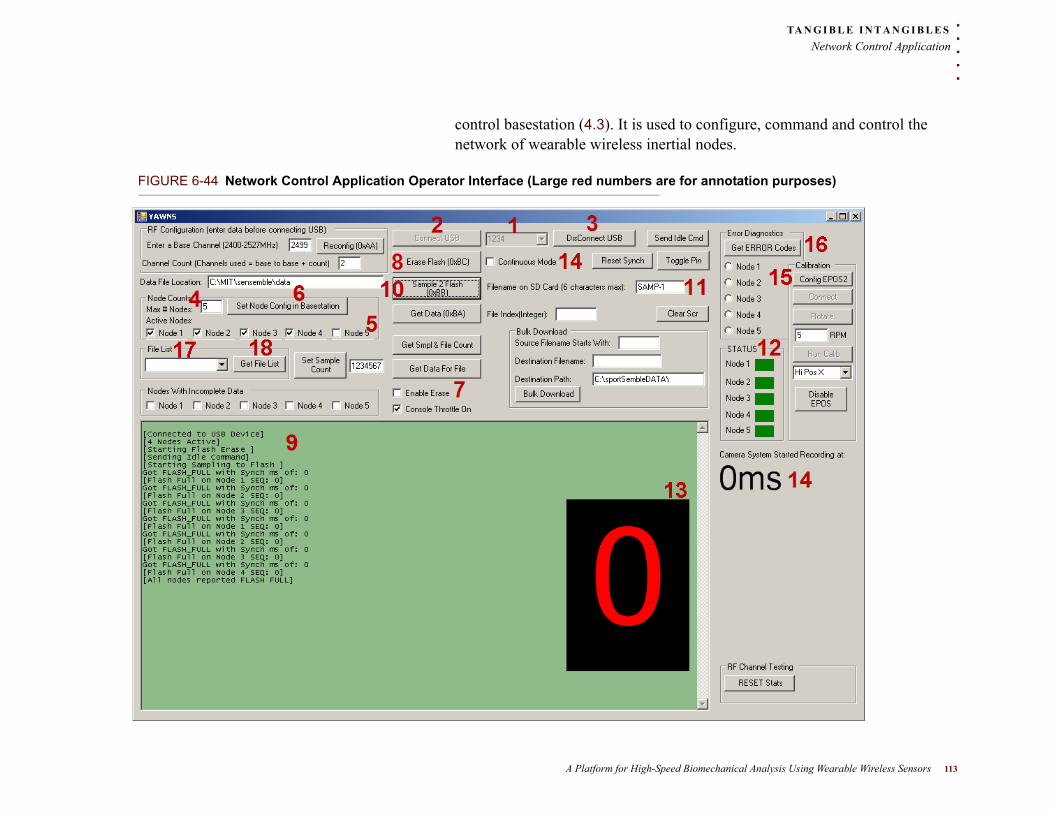
. . .
. .TA N G I B L E I N T A N G I B L E S
Network Control Application
control basestation (4.3). It is used to configure, command and control the network of wearable wireless inertial nodes.
FIGURE 6-44 Network Control Application Operator Interface (Large red numbers are for annotation purposes)
A Platform for High-Speed Biomechanical Analysis Using Wearable Wireless Sensors 113
TA N G I B L E I N T A N G I B L E S
Network Control Application
Documenting the functionality and operation of the network control application will heavily rely on FIGURE 6-44 and the red numbers that are present in the figure. The notation used to point at a specific number in the figure will simply be 6-26-<number>.
6 .1 .1 USB Connect ion
The first action an operator must do is choose the USB basestation from a list of available basestation devices, 6-26-1. While only one driver is used for our current basestation, this allows the USB driver (and hardware of the network control basestation) to be easily changed. With a selected USB basestation, the USB connection is configured and established by clicking the Connect USB button, 6-26-2. To disconnect, the operator clicks the Disconnect USB button, 6-26-3
6 .1 .2 Network Conf igurat ion
Setting the number of nodes in the network and which of these nodes are actively gathering data is part of network configuration. A text box is used to specify the number of nodes in the network (6-26-4). The maximum number of nodes supported by the RF protocol is 15 (enough to instrument every segment of the human body). However, all of the current software supports only 5 nodes needed to instrument a pitcher. A set of checkboxes (6-26-5) are used to specify which of the 5 nodes are active. Clicking the Set Node Config in Basestation (6-26-6) executes two of the commands documented in Section 5.1 and FIGURE 5-39 , the NUM_NODES_CMD and NODE_ACTIVE_CMD. This command is documented in Section 5.1. The main message area (6-26-9) will display text confirming that the network has been configured.
114 Michael T Lapinski
. . .
. .TA N G I B L E I N T A N G I B L E S
Network Control Application
6 .1 .3 Eras ing F lash
An erase of all data in the MCU’s internal flash and on the µSD card should be performed before beginning data gathering on a player. In order to avoid mistaken erasure of the data on all nodes (something that the author learned the hard way), a simple two phase process is employed. The first phase is to check the Enable Erase checkbox (6-26-7) that is placed geographically far away from the Erase Flash button, which can only be clicked with the prior checkbox checked. When clicked, a ERASE_FLASH command is generated and sent to the basestation. This command is documented in Section 5.1. The main message area (6-26-9) will display text confirming that the memory is being erased.
6 .1 .4 Sampl ing Gesture Data
With a configured network and clean memory to store gesture data, the operator enters a filename in the Filename on SD Card textbox (6-26-11) and clicks the Sample 2 Flash button (6-26-10). It is important to note that the maximum filename length is 6 characters, as dictated by the payload size of the wireless data packet. The click of the button triggers a SAMPLE_2_FLASH command to be sent to the basestation, along with the operator-entered filename.
During the sampling process, the operator observes two areas of the screen: the main message area (6-26-9) and the STATUS area (6-26-12). The main message area will display a message for every node that has replied that its flash is full. The STATUS area has a green/red box to the right of each node name. If the box is green, a packet has been received from that given node in the last 50ms. If the box is red, the node has not been heard from in the past 50ms. This is an excellent way of diagnosing which node(s) are misbehaving.
A Platform for High-Speed Biomechanical Analysis Using Wearable Wireless Sensors 115

TA N G I B L E I N T A N G I B L E S
Network Control Application
6 .1 .5 Cont inuous Sampl ing
The ability to continuously sample is desirable in order to better fit into the workflow and routines of athletes. Pitchers, for example, throw at their own pace and, as mentioned previously, a goal of the system is to fit into routine athletic activity as seamlessly as possible. Dictating when to start and stop impacts their, for lack of a better word, “mojo” and may affect performance.
Continuous mode is activated by checking the Continuous Mode checkbox (6-26-14), this sets the continuous mode byte in the outgoing packets that the basestation sends and enables continuous mode in the nodes, the mechanics of which are detailed in Section 5.3.0.6. While the checkbox is checked, the SEQUENCE_NUMBER will be incremented with every new dataset and displayed on the large red-on-black sequence number field (6-26-14). The reason that the sequence number field is so large and has a high contrast is to ease viewing when recording data in sunny outdoor environments. The system will stay recording in continuous mode until the Continuous Mode checkbox is unchecked. When this occurs, the current dataset recording completes, the SEQUENCE_NUMBER is reset to zero, and the system goes into the IDLE state.
6 .1 .6 Error Management
When errors do occur, they are recorded in the flash memory of each node, and the error handling subsystem is explained in Section 5.2.2. In order to retrieve errors, the operator first selects the node from the radio button list (6-26-15) and then clicks the Get ERROR Codes button (6-26-16).
When this occurs, a GET_ERROR_COUNT command is issued in order to retrieve the number of errors the specific node has experienced. Then a loop is executed, sending a GET_ERROR_CODE command from zero to the number of errors. As the error codes are transmitted back, each is displayed in the main message area (6-26-9) in hex.
116 Michael T Lapinski
. . .
. .TA N G I B L E I N T A N G I B L E S
Data Translation Application
6 .1 .7 Reading Node Contents
In order to see what datasets each node has recorded, there exists a mechanism to retrieve a list of files (datasets) from the node. The mechanics of the two commands used, GET_SAMPLE_CNT_CMD and GET_FILE_NAME are described in Sections 5.3.0.7 and 5.3.0.8, respectivley.
The operator first selects a node form the drop down menu (6-26-17) in the File List section of the GUI, then clicks the Get File List button (6-26-18). A Similar process is followed to that of retrieving an error list. A GET_SAMPLE_CNT_CMD count command is issued and a count of the number of datasets is obtained. Then a loop is executed from zero to this count, issuing a GET_FILE_NAME command with the index of the loop. For each iteration through the loop a filename is transmitted back by the node and printed in the main message area (6-26-9).
6 .1 .8 Opt ica l System Synchroniza t ion
The hardware connectivity and generation of synchronization offsets are described in Sections 4.3.1 and 5.1.1. The synchronization constant that is calculated and transmitted to the host PC is displayed under the Camera System Started Recording at label (6-26-14). If synchronization is ongoing, this data is normally recorded as part of normal data gathering procedures and entered into the database.
. . . . . . . . . . . . . . . . . . . . . . . . . . . . . . . . . . . . . . . . . . . . . . . . . . . . . . . . . . .6 . 2 D A T A T R A N S L A T I O N A P P L I C A T I O N
The data translation application is used in conjunction with the Data Translator (4.4, 5.4). The purpose of these two is to translate the data stored on
A Platform for High-Speed Biomechanical Analysis Using Wearable Wireless Sensors 117

TA N G I B L E I N T A N G I B L E S
Data Translation Application
µSD cards, as raw sectors, to something that is human readable and machine parseable. To connect the application via USB to the hardware translator, a customized version of an open source USB library, libusb[93], is used. A device driver matched to the EVK1101 (4.4) is compiled and installed on the host PC.
The same notation scheme used for FIGURE 6-44 in Section 6.1 will be used here, [FIGURE NUMBER]-[RED INDEX NUMBER].
118 Michael T Lapinski
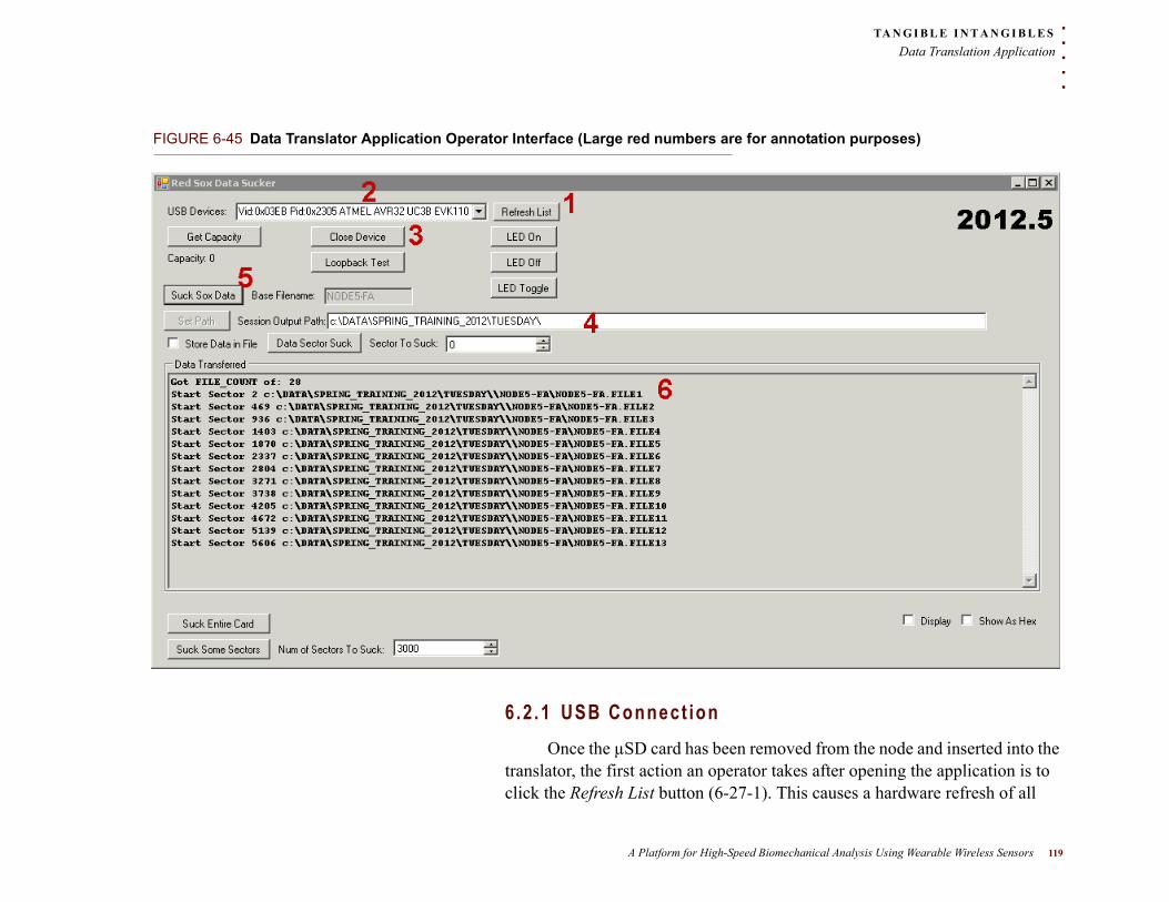
. . .
. .TA N G I B L E I N T A N G I B L E S
Data Translation Application
FIGURE 6-45 Data Translator Application Operator Interface (Large red numbers are for annotation purposes)
6 .2 .1 USB Connect ion
Once the µSD card has been removed from the node and inserted into the translator, the first action an operator takes after opening the application is to click the Refresh List button (6-27-1). This causes a hardware refresh of all
A Platform for High-Speed Biomechanical Analysis Using Wearable Wireless Sensors 119

TA N G I B L E I N T A N G I B L E S
Data Translation Application
USB devices that match the DeviceID of the Data Translator hardware and populates it into the USB Devices list (6-27-2). This list allows operating more then one data translator at a time to parallelize the time-consuming task of translating data. The operator selects the desired device and clicks the Open/Close Device button (6-27-3). This button toggles its label between Open Device and Close Device, depending on system state. If the device is already opened, the only possible action is to close it, and vice versa if it is open.
6 .2 .2 Trans la t ing Data
The operator specifies a directory path to where the data from the µSD card should be translated to in the Session Ouput Path text field (6-27-4) and clicks the Suck Data button (6-27-5).
The application goes into a loop that requests one sector at a time, the mechanics of which are described in Section 5.4.
Sector 1, as detailed in Section 5.3.0.5, is a special sector and contains metadata regarding which node the card came from(NODE_ID), its location on the body (NODE_LOCATION) and how much data is present on the card (DATASET_COUNT). The DATASET_COUNT dictates how many datasets the application should expect.
Based on the Session Output Path, NODE_ID and NODE_LOCATION, a new directory is created on disk. The naming conventions for this directory is [Session Output Path]\NODE[NODE_LOCATION]-NODE_ID\. For example, and as can be seen in the main message area of the application (6-27-6), the Session Output Path is C:\DATA\SPRING_TRAINING_2012\TUESDAY and the read NODE_LOCATION is 5 and the NODE_ID is FA. This yields the directory C:\DATA\SPRING_TRAINING_2012\TUESDAY\NODE5-FA\ for storing all data from this card.
120 Michael T Lapinski

. . .
. .TA N G I B L E I N T A N G I B L E S
Data Translation Application
Once sector 1 has been processed, the application begins to sequentially request sectors from the data translator. With each received sector, it reads 28 bytes at a time and processes the contents. 28 bytes are read because this is the length of the data packets that are placed onto the card by the nodes, and the format and information regarding card writing is located in Section 5.3.0.5.
Once 28 bytes are read, 4 HEADER_BYTES are checked to determine what kind of data is contained in the given packet. There are three types of packets: header, inertial and magnetometer.
The first packet for any gesture dataset is a header packet that contains the 6-character FILENAME and SEQUENCE_NUMBER. These two are used to create 4 different files, with different DATATYPEs for each recorded gesture.
1 Synchronization File - SEQDATA - Timestamp and synchronization
data
2 High Range Inertial File - NO DATATYPE STRING - High range X, Y, Z
and Pitch, Roll, Yaw data is contained in this file
3 Low Range Inertial File - LOWG - High range X, Y, Z and Pitch, Roll,
Yaw data is contained in this file
4 Magnetometer File - COMPASS - Magnetometer X, Y, Z data is
contained in this file
Additionally, when a header packet is encountered, a global FILE_COUNTER is incremented by one. The naming convention for the filenames is:
NODE[NODE_LOCATION]-[NODE_ID].FILE[FILE_COUNTER].[FILENAME].SEQ[SEQUENCE_NUMBER].[DATATYPE].txt
An example of the four files for a single gesture is:
NODE1-AC.FILE4.ZupDn.SEQ0.SEQDATA.txt - Synchronization
NODE1-AC.FILE4.ZupDn.SEQ0.txt - High range inertial
A Platform for High-Speed Biomechanical Analysis Using Wearable Wireless Sensors 121

TA N G I B L E I N T A N G I B L E S
Data Translation Application
NODE1-AC.FILE4.ZupDn.SEQ0.LOWG.txt - Low range inertial
NODE1-AC.FILE4.ZupDn.SEQ0.COMPASS.txt - Magnetometer
The header packet also contains a global timestamp, this timestamp is written out to the Synchronization file and is later used to perform a global synchronization for all data gathered. Once the four files are created and opened, processing of data packets can begin.
If the packets’ HEADER_BYTES match an inertial packet, the encoded inertial data from high range X, Y, Z and pitch, roll, yaw and low range X, Y, Z and pitch, roll, yaw is decoded. This data is output in comma-separated-value (CSV) format into the low range inertial data file for low range data and the high range inertial data file for the high range data.
If the HEADER_BYTES contain the magnetometer code, magnetometer data is decoded from the packet and written out to the magnetometer file.
When the current sector has been iterated through in 28 byte increments, the next sector is requested from the translator, and the same process is followed for packets in the sector. If a new header packet (representing the next recorded gesture) is encountered, the current data files are closed and new ones, based on the information in the packet, are created.
The translation process terminates when a pre-determined number of sectors are read without a header packet being read from the card. When this occurs, a message is written out to the main message area (6-27-6).
122 Michael T Lapinski
. . .
. .TA N G I B L E I N T A N G I B L E S
Data Model
. . . . . . . . . . . . . . . . . . . . . . . . . . . . . . . . . . . . . . . . . . . . . . . . . . . . . . . . . . .6 . 3 D A T A M O D E L
It is important to understand the inherent data demands and data complexity of a system such as this. The system’s data storage must be capable of storing data for hundreds, possibly thousands, of gestures for hundreds of players. Further, each eight second gesture consists of roughly 40,000 raw datapoints and 40,000 calibrated datapoints. Not only this, but there are several different pieces of metadata that exists for each gesture and each sample. This amount of data quickly grows into millions of records, hence it is easy to see that managing all of it is not a trivial task. A model to store all of this data has been evolving since the project’s inception in 2008 and has grown from 9 tables to 25 today.
This data model can divided into five logical categories; Player, Session, Gesture, Node and Visual3D. These are illustrated in FIGURE 6-46 . These categories partially reflect the taxonomy introduced in Sections 3.1.0.1, 3.1.0.2 and 3.1.0.3. Each category and its associated tables, accompanied by a human-readable figure, will be presented in the following sections.
Before delving into the data model, it is important to note that while most import and insertion of the raw sensor data is automated, there are several pieces of data that are manually entered into the database via the Data Processing Application. These include the biometric and anthropometric information and measurements that are gathered for each player before each session. Additionally, each gesture, be it a pitch or swing, has metadata associated with it that is also entered into the database via the Data Processing Application. Here the backend data model is presented; the process of recording this data in our logbook is presented in the Experimental Methods Chapter that follows this chapter.
A Platform for High-Speed Biomechanical Analysis Using Wearable Wireless Sensors 123
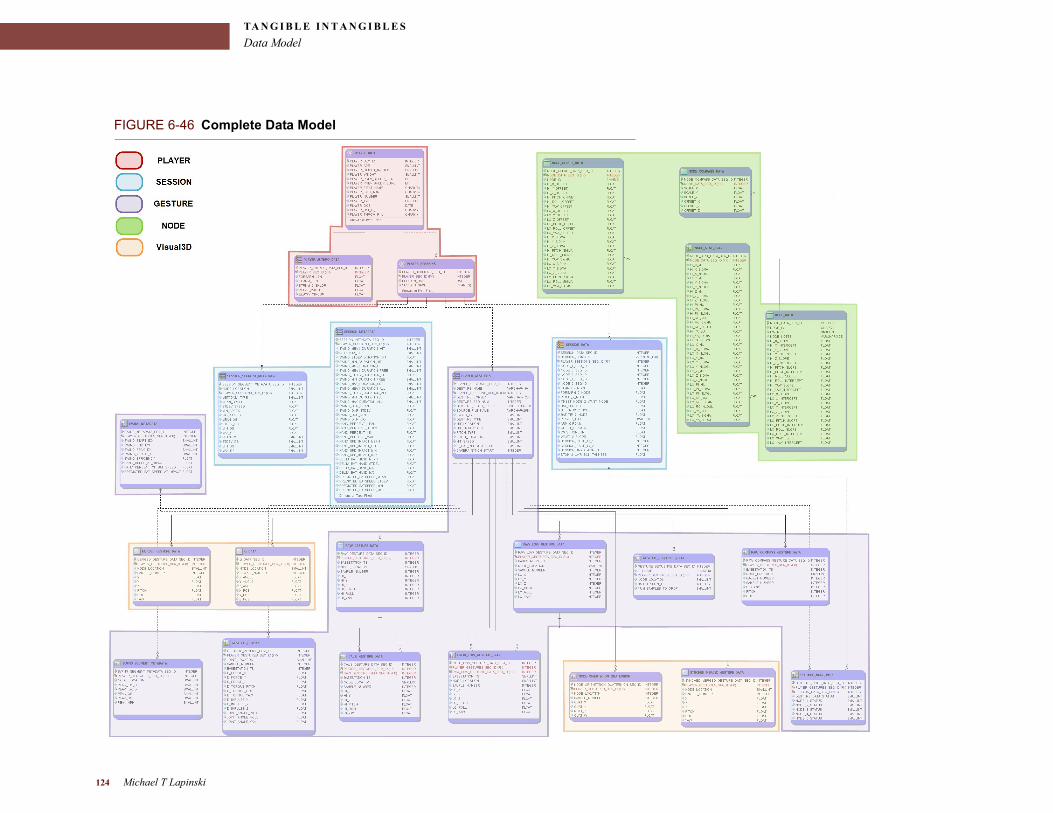
TA N G I B L E I N T A N G I B L E S
Data Model
FIGURE 6-46 Complete Data Model
124 Michael T Lapinski

. . .
. .TA N G I B L E I N T A N G I B L E S
Data Model
6 .3 .1 P layer Data Model
The player data model consists of two tables, PLAYER_INFO and PLAYER_ANTHRO_DATA. The PLAYER_INFO table contains general biometric data; the specific information that is present in this table mirrors numbered points 1 to 12 in Section 3.1.0.1. PLAYER_ANTHRO_DATA contains anthropometric information, namely the information outlined by numbered points 13 to 18 in the previously-mentioned section. A mandatory one-to-one relationship exists between these tables, meaning that for every player, there must exist anthropometric data. The primary key of the PLAYER_INFO, PLAYER_SEQ_ID, is a unique identifier for all Players, and is a foreign key in PLAYER_ANTHRO_DATA.
FIGURE 6-47 Player Data Model
A Platform for High-Speed Biomechanical Analysis Using Wearable Wireless Sensors 125
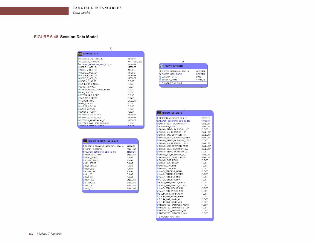
TA N G I B L E I N T A N G I B L E S
Data Model
FIGURE 6-48 Session Data Model
126 Michael T Lapinski
. . .
. .TA N G I B L E I N T A N G I B L E S
Data Model
6 .3 .2 Sess ion Data Model
The Session concept is defined and described Section 3.1.0.2; the data model consists of four tables, PLAYER_SESSIONS, SESSION_DATA, SESSION_SEGMENT_METADATA and SESSION_METADATA.
PLAYER_SESSIONS has a foreign key from PLAYER_INFO, and its relationship to PLAYER_INFO is, from PLAYER_INFO to PLAYER_SESSIONS, one to many. This indicates that for one Player, there exist one or more Sessions. This table contains its primary key, PLAYER_SESSION_SEQ_ID, the session name and session date (number points 1 and 2 in Section 3.1.0.2). The bulk of the information outlined in the numbered list of the Session description is contained in the helper table SESSION_DATA.
PLAYER_SESSION_SEQ_ID is a foreign key in SESSION_DATA, and as the relationship between these two tables is mandatory one-to-one, session data must exist for each Session. The data contained in this table is outlined in numbered points 3 through 21 in Section 3.1.0.2.
The two metadata tables contain post-processed data and statistics that are generated on a per-session level. SESSION_METADATA reflects statistics generated inter-node, for example, the mean delta between peak angular velocity for the hand and forearm nodes. SESSION_SEGMENT_METADATA contains statistics that are on a per-node basis. For example, the mean G-Force experienced by the hand node for this Session. Data for these tables is generated by the Analytics Engine described in Section 9.3 and will be covered in more detail in that section.
6 .3 .3 Gesture Data Model
Core data directly related to what each nodes sensors read (Sections 4.1.1 and 4.1.2) and is later translated to the filesystem (Section 6.2.2) is stored
A Platform for High-Speed Biomechanical Analysis Using Wearable Wireless Sensors 127
TA N G I B L E I N T A N G I B L E S
Data Model
in five tables: PLAYER_GESTURES, RAW_GESTURE_DATA, RAW_LOW_GESTURE_DATA, GESTURE_SEQUENCE_DATA and RAW_COMPASS_GESTURE_DATA16.
16RAW_COMPASS_GESTURE_DATA is a misnomer, since magnetometer data is gathered. It is a naming relic from previous hardware [7] that used a digital compass in place of a magnetometer.
The root table, PLAYER_GESTURES, has a foreign key from the PLAYER_SESSIONS table and a one-to-many relationship exists between the two, indicating that one Session is associated with multiple Gestures. PLAYER_GESTURES has its own primary key, PLAYER_GESTURES_SEQ_ID, whose purpose will be clear once all tables related to Gesture data are described. As with Player and Session, the data stored in the PLAYER_GESTURES table also mirrors what is enumerated in the Gesture taxonomy section (3.1.0.3), specifically, numbered points 1 through 13 in that section. This is general information pertaining to the physical gesture, and the actual data sampled from the sensors is stored in the RAW_* tables.
The RAW_* tables are directly correlated with the four files per gesture that are created in the filesystem by the translator (6.2.2). Each of these has a many-to-one relationship with PLAYER_GESTURES, meaning that each of the many samples of data that is inserted are related to only one Gesture. In order to identify what gesture the data is part of, PLAYER_GESTURES_SEQ_ID has a foreign key in each RAW_* table.
Data from the High Range Inertial File is inserted into the RAW_GESTURE_DATA table. Data from the Low Range Inertial File is inserted into the RAW_LOW_GESTURE_DATA. Data from the Synchronization File is inserted into the GESTURE_SEQUENCE_DATA table. And, finally, data from the Magnetometer File is inserted into the RAW_COMPASS_GESTURE_DATA16 table.
128 Michael T Lapinski
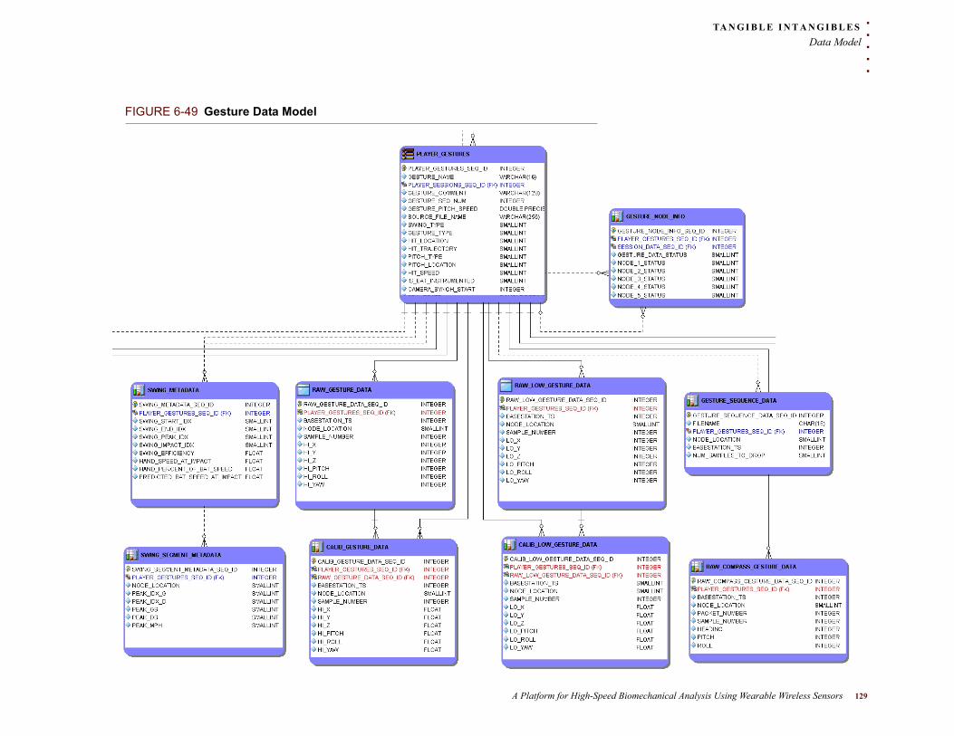
. . .
. .TA N G I B L E I N T A N G I B L E S
Data Model
FIGURE 6-49 Gesture Data Model
A Platform for High-Speed Biomechanical Analysis Using Wearable Wireless Sensors 129

TA N G I B L E I N T A N G I B L E S
Data Model
The naming convention of RAW indicates that the data stored is in a raw format. In the case of RAW_GESTURE_DATA and RAW_LOW_GESTURE_DATA, it is in fact raw analog data that needs to be converted using calibration constants (described in Section 4.2). In order to keep both raw and calibrated data, for archival purposes and in case re-calibration becomes necessary, the calibrated data is inserted into two new tables, aptly named CALIB_GESTURE_DATA and CALIB_LOW_GESTURE_DATA. The GESTURE_SEQUENCE_DATA and RAW_COMPASS_GESTURE_DATA16 do not have matching CALIB_ tables because this data is in a final format. However, post-processing of this data does occur to calculate heading, from RAW_COMPASS_GESTURE_DATA, and node synchronization offsets, from GESTURE_SEQUENCE_DATA. This will be addressed in Section 7.2.
The third tier of storage for gestures are the two *_METADATA tables and are similar in purpose to the *_METADATA tables for Sessions. The “SWING” name portion of the tables SWING_METADATA and SWING_SEGMENT_METADATA is a misnomer because the metadata in these tables is not only related to swings. Initially, it only was swing related (i.e. for batters) and as the system evolved the table was used for both swings and pitches. SWING_METADATA contains Gesture level information, such as the start and end samples of the given gesture. SWING_SEGMENT_METADATA contains segment-specific information, such as the peak angular velocity for a given segment for a given gesture.
6 .3 .4 Node Data Model
Section 4.2 describes’, in depth, the calibration process each axis of each node and the process of generating calibration constants for each axis. The generated constants, along with their coefficients of determination (FIGURE 4-35 ), statistical noise data and magnetometer calibration data are all stored as part of the Node Data Model. These four tables are shown in FIGURE 6-50
130 Michael T Lapinski
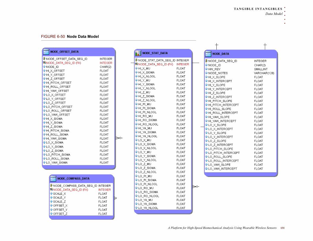
. . .
. .TA N G I B L E I N T A N G I B L E S
Data Model
FIGURE 6-50 Node Data Model
A Platform for High-Speed Biomechanical Analysis Using Wearable Wireless Sensors 131
TA N G I B L E I N T A N G I B L E S
Data Model
The calculated linear calibration constants are stored in the NODE_DATA table. These include slope and Y intercept for each inertial axis, a unique node identifier and a primary key, NODE_DATA_SEQ_ID, that will be a foreign key to link data to a specific node in the other tables.
NODE_COMPASS_DATA16 contains scale and offset values for each of the three axes of the magnetometer. NODE_DATA_SEQ_ID is a foreign key to identify which node this data is for. The relationship between this table and NODE_DATA is one-to-one.
The NODE_OFFSET_DATA table has a “dual personality”, as it contains offset data and coefficients of determination for each inertial axis. Offset data is occasionally calculated for inertial sensors that drift severely over short periods of time. The coefficients of determination (R2) are calculated at calibration time to examine the goodness of the correlation and are stored here for future analysis. As with the previous table, NODE_OFFSET_DATA also has a foreign key of NODE_DATA_SEQ_ID, which establishes the data uniqueness and a one-to-one relationship with NODE_DATA.
NODE_STAT_DATA is information used for generating covariance statistics that are used by orientation estimation algorithms and kinematic estimation Kalman filters. There are three components for each inertial axis, μ sigma and the negative log likelihood. NODE_DATA_SEQ_ID is a foreign key and the two tables have a one-to-one relationship.
6 .3 .5 V isua l3D Data Model
Visual3D [65] and its connection to this work is briefly described in Section 3.4 and an in-depth description is featured in Section 9.7.1. The custom plug-in developed to import inertial data uses inertial data to compute dynamics and previously calculated kinematic Q-Data to drive the upper body model.
132 Michael T Lapinski
. . .
. .TA N G I B L E I N T A N G I B L E S
Data Model
The Q-Data is stored in the Q_DATA table. It contains the three Euler angles that represent joints, which dictate segment-to-segment rotations to set the orientation of each body segment. Additionally, X, Y, Z translation data is stored for any segments that are allowed to translate in 3D space. Each record in the table represents one calculated orientation between two segments (one joint) for one time step. PLAYER_GESTURES_SEQ_ID,from the PLAYER_GESTURES table, is a foreign key, establishing a mandatory one-to-one relationship between these two tables.
The low range and high range data exists in separate tables and as separate data streams for each inertial axis and require fusion (Section 9.5) before the Visual3D plug-in can access them via the SYNCHED_MERGED_GESTURE_DATA table. Each low range and high range inertial axis is fused and placed into its respective column. This data is stored on a per segment, per sample basis for each PLAYER_GESTURES_SEQ_ID, a foreign key in this table. The MERGED_GESTURE_DATA table has the same structure and a similar purpose. The difference between the two is that synchronization offsets from the GESTURE_SEQUENCE_DATA, which contains calculated offset information for each node in the network.
Segment orientations are calculated as intermediate data and stored in the NODE_ORIENTATION_QUATERNION table. The four parts that represent a Quaternion [105] are stored along with which segment (NODE_LOCATION) and sample number the orientation is for. PLAYER_GESTURES_SEQ_ID is a foreign key and establishes a one-to-one relationship.
A Platform for High-Speed Biomechanical Analysis Using Wearable Wireless Sensors 133
TA N G I B L E I N T A N G I B L E S
Data Processing and Import Application - Operator View
6 . 4 D A T A P R O C E S S I N G A N D I M P O R T
. . . . . . . . . . . . . . . . . . . . . . . . . . . . . . . . . . . . . . . . . . . . . . . . . . . . . . . . . . .A P P L I C A T I O N - O P E R A T O R V I E W
Details of the data processing application will be broken up into the two logical viewpoints that reflect the different types of interaction with the application, the user and the operator. This section will focus on the operator and will cover creation of players, sessions, gestures, nodes and the process of importing the data provided by the translator into the relational database.
6 .4 .1 Database Connect iv i ty
As the system has evolved, there have been three different instances of the database, 2009, 2010 and 2012. All three have slight differences in data structure, but backwards compatibility has been built into the Data Processing Application. Only the latest schema is considered here, as it has the most features. The same notation will be used here to identify different graphical features that was used in Sections 6.1 and 6.2. To connect to the database, the operator selects the desired database version in the Database Version radio button group (6-33-1) and then clicks the Connect DB button (6-33-2). To change databases, the operator clicks the Disconnect DB button (6-33-3) and follows the process just outlined.
134 Michael T Lapinski
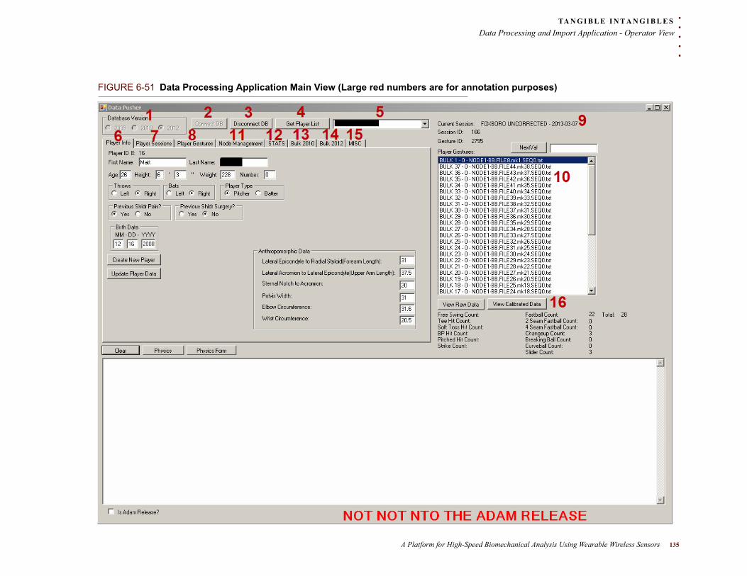
. . .
. .TA N G I B L E I N T A N G I B L E S
Data Processing and Import Application - Operator View
FIGURE 6-51 Data Processing Application Main View (Large red numbers are for annotation purposes)
A Platform for High-Speed Biomechanical Analysis Using Wearable Wireless Sensors 135
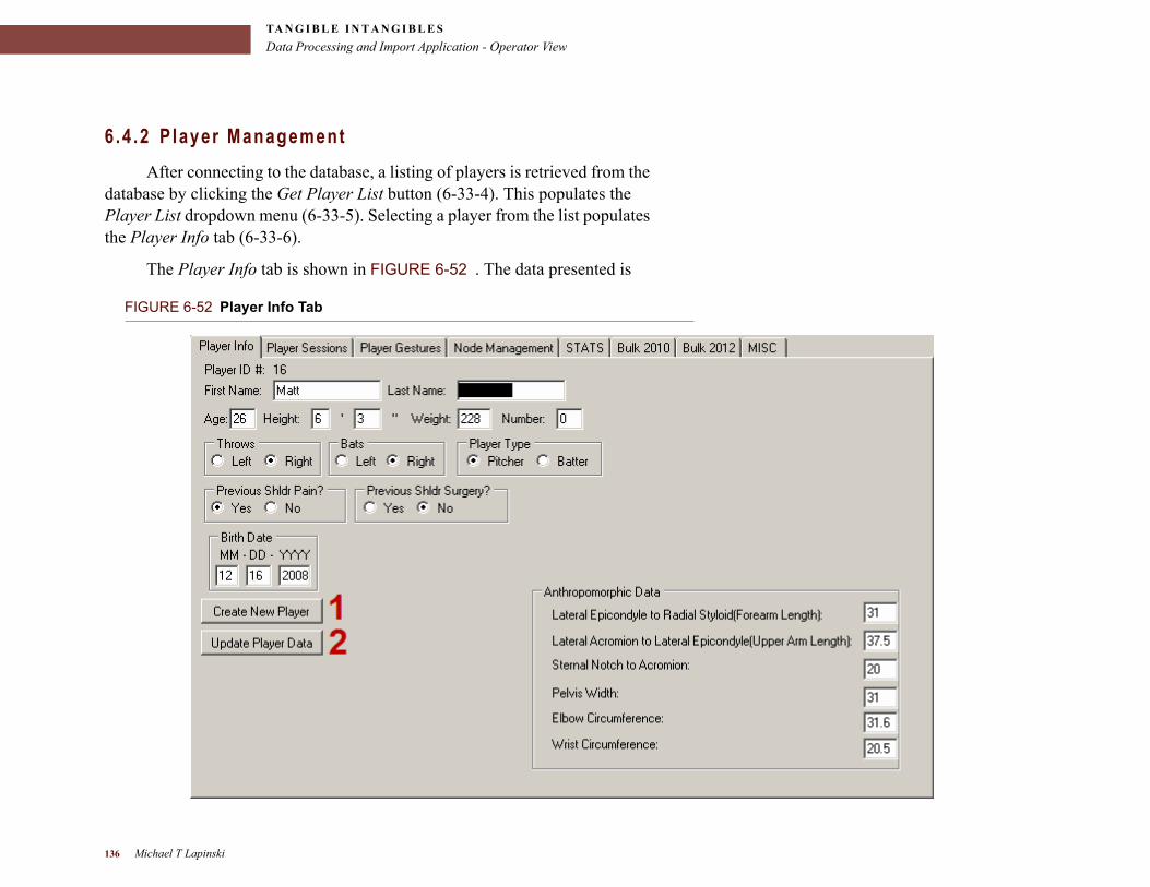
TA N G I B L E I N T A N G I B L E S
Data Processing and Import Application - Operator View
6 .4 .2 P layer Management
After connecting to the database, a listing of players is retrieved from the database by clicking the Get Player List button (6-33-4). This populates the Player List dropdown menu (6-33-5). Selecting a player from the list populates the Player Info tab (6-33-6).
The Player Info tab is shown in FIGURE 6-52 . The data presented is
FIGURE 6-52 Player Info Tab
136 Michael T Lapinski
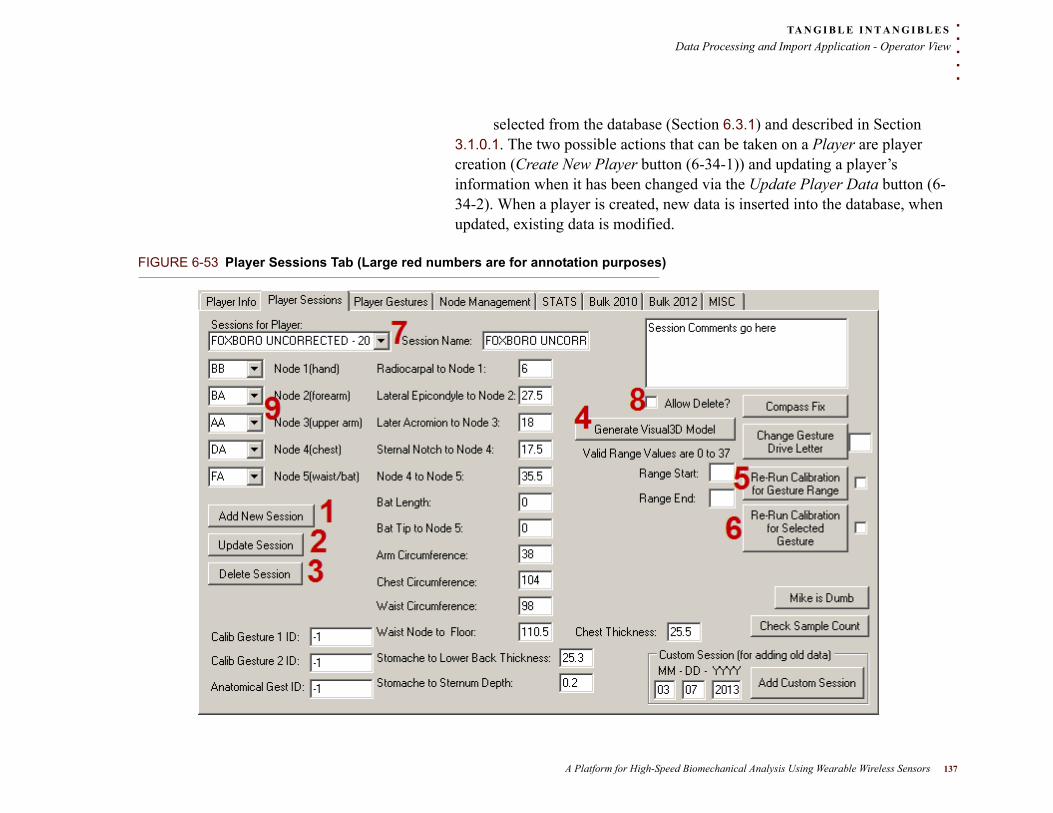
. . .
. .TA N G I B L E I N T A N G I B L E S
Data Processing and Import Application - Operator View
selected from the database (Section 6.3.1) and described in Section 3.1.0.1. The two possible actions that can be taken on a Player are player creation (Create New Player button (6-34-1)) and updating a player’s information when it has been changed via the Update Player Data button (6-34-2). When a player is created, new data is inserted into the database, when updated, existing data is modified.
FIGURE 6-53 Player Sessions Tab (Large red numbers are for annotation purposes)
A Platform for High-Speed Biomechanical Analysis Using Wearable Wireless Sensors 137
TA N G I B L E I N T A N G I B L E S
Data Processing and Import Application - Operator View
6 .4 .3 Sess ion Management
Session management actions are contained under the Player Sessions tab (6-33-7); the tab is presented in FIGURE 6-53 . As with Player Info, the presented information is described in Section 3.1.0.2. An operator specifies a session name, selects which nodes are located on which body segment (6-35-9) and measured anthropometric data. There are options to create (6-35-1), update (6-35-2) and delete (6-35-3) existing sessions. Deletion is a two phase process and requires the Allow Delete? checkbox (6-35-8) to be checked.
Additionally, the output of the Visual3D model file, which is based on the measured anthropometric data for each player and session, is executed by clicking the Generate Visual3D Model button (6-35-4). Sessions are selected by choosing them from the Sessions for Player dropdown menu (6-35-7). When a session is selected, the information in the Main View (FIGURE 6-51 ) for the Current Session (6-33-9) and the Player Gestures list (6-33-10) is updated with the gestures for the selected session.
There are two features that make use of the raw data that is kept in the database, the ability to re-run calibration. If there are any issues with a calibration and new calibration constants are regenerated, any previously gathered data can be reprocessed, making it usable for future study. There is a two phase process for recalibrating, similar to deleting sessions. Next to the Re-Run Calibration for Selected Gesture (6-33-6) there is a checkbox that needs to be checked in order for the recalibration to run. There is also an option to specify a range of gestures to be recalibrated and to recalibrate a group of gestures (6-35-5).
6 .4 .4 Gesture Handl ing
Gesture management falls into two categories: importing data into the database and annotating, classifying and managing the gestures once they have been imported.
138 Michael T Lapinski
. . .
. .TA N G I B L E I N T A N G I B L E S
Data Processing and Import Application - Operator View
6.4 .4 .1 Gesture Import Process
The interface for the import process is available via the Bulk 2012 tab (6-33-14). As documented in Section 6.2.2, there are four files generated by the Data Translator for each recorded gesture, and in order to load this data into the database, the operator clicks the Add Files button (6-50-1). This brings up a file selection dialog box and the operator selects any one of the four files for an individual gesture from one node. The operator can use the Shift+Click windows feature to select multiple individual files from gestures. Once the dialog is closed, the files are added to the File List Area (6-36-2).
The reason that, for each gesture, only one file from one node needs to be selected is because the algorithms that load data are built to take advantage of the specified file format and node segment placement information that is encoded under the Player Session tab (6-33-7).
Once the Import Bulk Gestures button (6-36-3) is clicked, a series of checks and verifications occurs based on Session data. These rely on the file and directory structure detailed in Section 6.2.2. The algorithm first checks the node ID’s and node locations (6-49-9), and looks for appropriate directories. For example, for the node configuration depicted in FIGURE 6-53 , the expected directory names are: NODE1-BB, NODE2-BA, NODE3-AA, NODE4-DA and NODE5-FA. For each gesture in the gesture list (6-36-2), a root directory, sequence number and filename (that is specified by the operator at data gathering time) are parsed out. For the last gesture in the list in FIGURE 6-54 , the parsed root directory is:
C:\MIT\sportsemble\DATA\2012_TESTING\COMPASS_TEST_APR11\
and the parsed sequence number is 0 and the parsed filename is down1. This information is used to search for files, following the directory structure and node naming rules.
A Platform for High-Speed Biomechanical Analysis Using Wearable Wireless Sensors 139
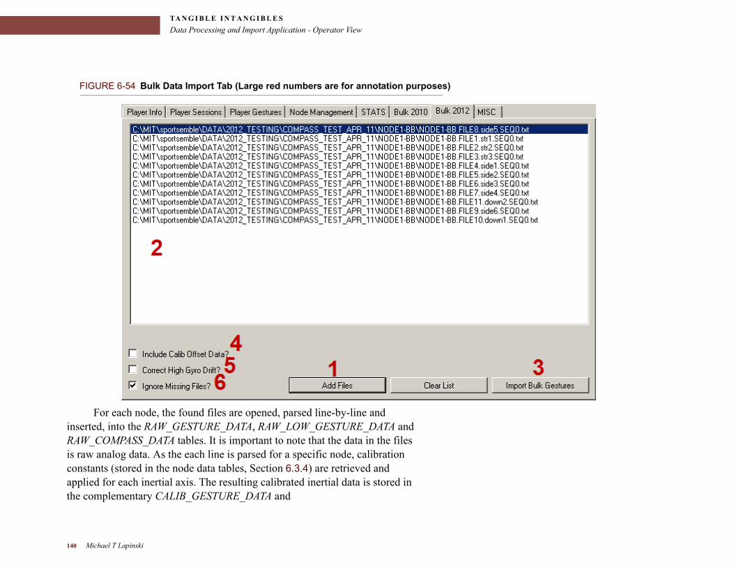
TA N G I B L E I N T A N G I B L E S
Data Processing and Import Application - Operator View
FIGURE 6-54 Bulk Data Import Tab (Large red numbers are for annotation purposes)
For each node, the found files are opened, parsed line-by-line and inserted, into the RAW_GESTURE_DATA, RAW_LOW_GESTURE_DATA and RAW_COMPASS_DATA tables. It is important to note that the data in the files is raw analog data. As the each line is parsed for a specific node, calibration constants (stored in the node data tables, Section 6.3.4) are retrieved and applied for each inertial axis. The resulting calibrated inertial data is stored in the complementary CALIB_GESTURE_DATA and
140 Michael T Lapinski

. . .
. .TA N G I B L E I N T A N G I B L E S
Data Processing and Import Application - Operator View
CALIB_LOW_GESTURE_DATA tables. If data is not available from all five nodes, the default behavior of the system is to fail and the abort the import process. This behavior can be overridden by checking the Ignore Missing Files? checkbox (6-36-6). Application of inertial sensor-specific offsets that are present in the node data model can be turned on and off by clicking the Include Calib Offset Data? (6-36-4) and Correct High Gyro Drift? (6-36-5) checkboxes.
6.4 .4 .2 Gesture Annotat ion and Management
The loading of gesture data is a preliminary step in having data ready for analysis. The next step is to annotate the data. Detailed annotation is covered in Sections 7.5; here the user interface for doing so will be described.
A Platform for High-Speed Biomechanical Analysis Using Wearable Wireless Sensors 141
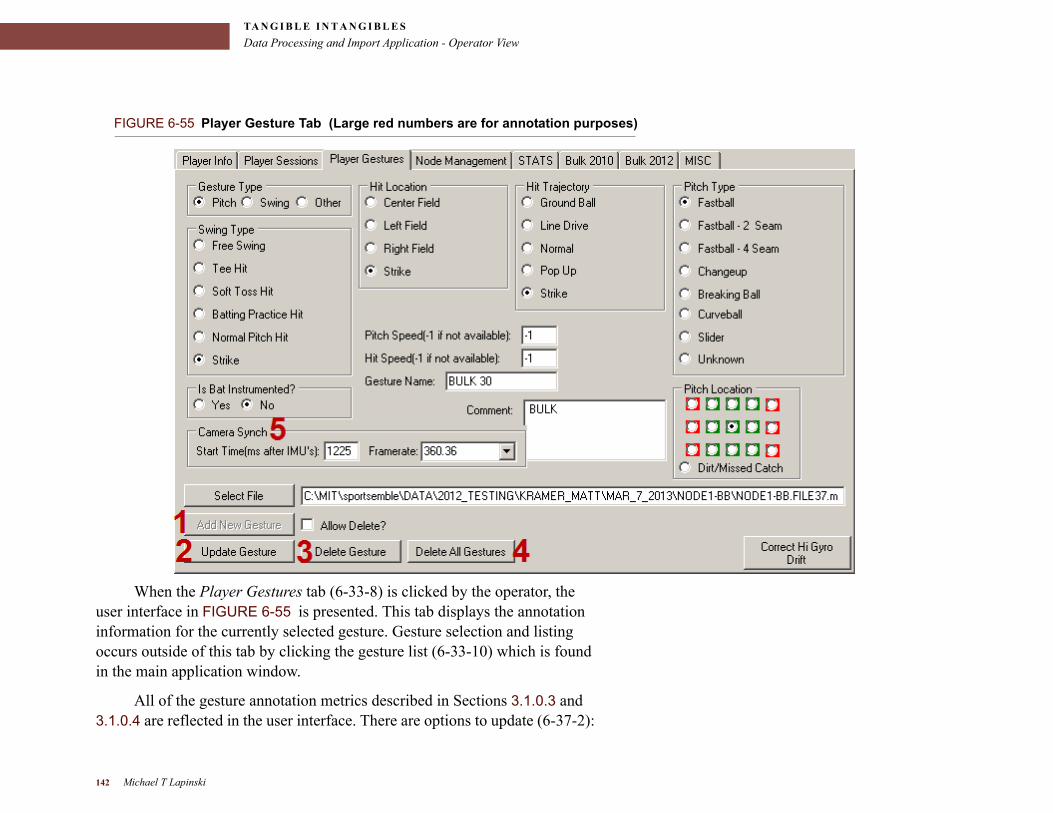
TA N G I B L E I N T A N G I B L E S
Data Processing and Import Application - Operator View
FIGURE 6-55 Player Gesture Tab (Large red numbers are for annotation purposes)
When the Player Gestures tab (6-33-8) is clicked by the operator, the user interface in FIGURE 6-55 is presented. This tab displays the annotation information for the currently selected gesture. Gesture selection and listing occurs outside of this tab by clicking the gesture list (6-33-10) which is found in the main application window.
All of the gesture annotation metrics described in Sections 3.1.0.3 and 3.1.0.4 are reflected in the user interface. There are options to update (6-37-2):
142 Michael T Lapinski
. . .
. .TA N G I B L E I N T A N G I B L E S
Data Processing and Import Application - Operator View
delete individual (6-37-3) and delete all gestures (6-37-4). Deletion is, again, a two phase process. The functionality to add gestures has been disabled in this interface (6-37-1) and the Bulk 2012 tab is relied upon for data import. Additionally, there is a Camera Synch (6-37-5) area in the interface that allows annotation of optical system synchronization data (Sections 4.3.1, 5.1.1 and 6.1.8). All of this annotation data leverages the Gesture Data Model described in Section 6.3.3.
6 .4 .5 Misce l laneous Operator Features
In order to allow Matlab and C/C++ interfaces into the data model, a need arose for each of the API’s that were developed to determine if a gesture’s data was considered usable (able to be processed) and if an individual node’s data was considered usable. Algorithms were developed to calculate the validity of a gesture and the node data; activation and results display is triggered via buttons under the MISC tab (6-33-15). These algorithms ensure that each node has data present in the database, and the metadata generated by them allows the external code to ascertain if data should be expected from a specific node for a specific gesture.
Initially, the status of all nodes and a gesture is labeled as unknown. In order to check the data for a gesture or all gestures in a session, the a radio button in the Automated Node Data Checking radio group (6-38-1) must be chosen and the Check Node Data (6-38-2) button must be clicked. The checks are performed, and status information is inserted into the GESTURE_NODE_INFO database table. When selecting a gesture in the gesture selection area in the main application view (6-33-10), the populated information is retrieved and the Gesture Node Data Status radio groups (6-38-3) are updated. If there is a need for the operator to update the information manually, the radio groups can be changed, and clicking the Update button (6-38-4) will update the information in the database.
A Platform for High-Speed Biomechanical Analysis Using Wearable Wireless Sensors 143
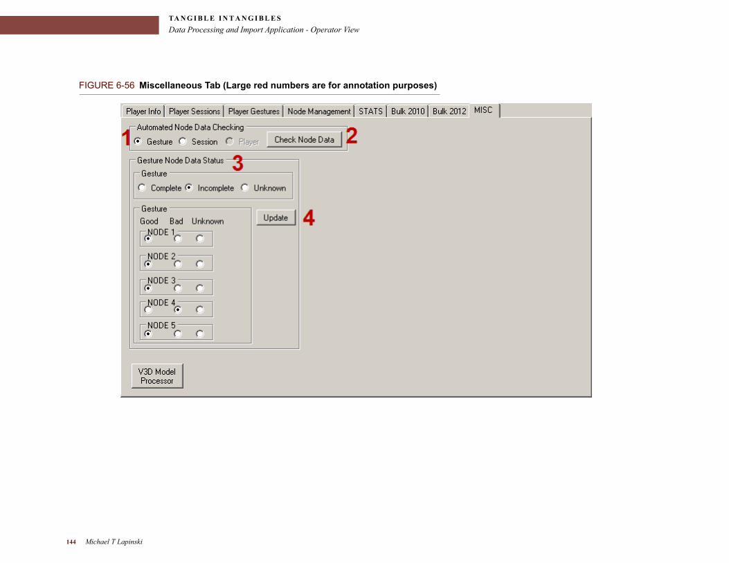
TA N G I B L E I N T A N G I B L E S
Data Processing and Import Application - Operator View
FIGURE 6-56 Miscellaneous Tab (Large red numbers are for annotation purposes)
144 Michael T Lapinski
. . .
. .TA N G I B L E I N T A N G I B L E S
. Data Processing and Import Application - User View
6 . 5 . D A T A P R O C E S S I N G A N D I M P O R T
. . . . . . . . . . . . . . . . . . . . . . . . . . . . . . . . . . . . . . . . . . . . . . . . . . . . . . . . . . .A P P L I C A T I O N - U S E R V I E W
Before presenting the user view of the Data Processing and Import Application, it makes more sense to examine the experimental methods that an operator uses to gather data. These methods are presented in Chapter 7
A Platform for High-Speed Biomechanical Analysis Using Wearable Wireless Sensors 145

TA N G I B L E I N T A N G I B L E S
. Data Processing and Import Application - User View
146 Michael T Lapinski
. . .
. .E X P E R I M E N T A L M E T H O D S
EXPERIMENTAL
. . . .
. . . . . . . . . . . . . . . . . . . . . . . . . . . . . . . . . . . . . .METHODS
This chapter is, for the average reader, possibly the most important and could almost be considered a starting point. It describes the way in which the realized network is used to gather data from players and how that data is preprocessed for analysis.
A Platform for High-Speed Biomechanical Analysis Using Wearable Wireless Sensors 147
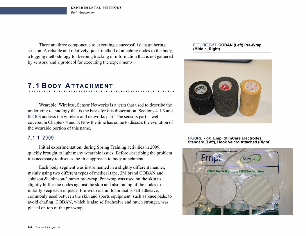
E X P E R I M E N T A L M E T H O D S
Body Attachment
FIGURE 7-57 COBAN (Left) Pre-Wrap (Middle, Right)
There are three components to executing a successful data gathering session: A reliable and relatively quick method of attaching nodes to the body, a logging methodology for keeping tracking of information that is not gathered by sensors, and a protocol for executing the experiments.
. . . . . . . . . . . . . . . . . . . . . . . . . . . . . . . . . . . . . . . . . . . . . . . . . . . . . . . . . . .7 . 1 B O D Y A T T A C H M E N T
Wearable, Wireless, Sensor Networks is a term that used to describe the underlying technology that is the basis for this dissertation. Sections 4.1.3 and 5.2.5.8 address the wireless and networks part. The sensors part is well covered in Chapters 4 and 5. Now the time has come to discuss the evolution of the wearable portion of this name.
FIGURE 7-58 Empi StimCare Electrodes, Standard (Left), Hook Velcro Attached (Right)
7 .1 .1 2009
Initial experimentation, during Spring Training activities in 2009, quickly brought to light many wearable issues. Before describing the problem it is necessary to discuss the first approach to body attachment.
Each body segment was instrumented in a slightly different manner, mainly using two different types of medical tape, 3M brand COBAN and Johnson & Johnson/Cramer pre-wrap. Pre-wrap was used on the skin to slightly buffer the nodes against the skin and also on top of the nodes to initially keep each in place. Pre-wrap is thin foam that is self adhesive, commonly used between the skin and sports equipment, such as knee pads, to avoid chafing. COBAN, which is also self adhesive and much stronger, was placed on top of the pre-wrap.
148 Michael T Lapinski
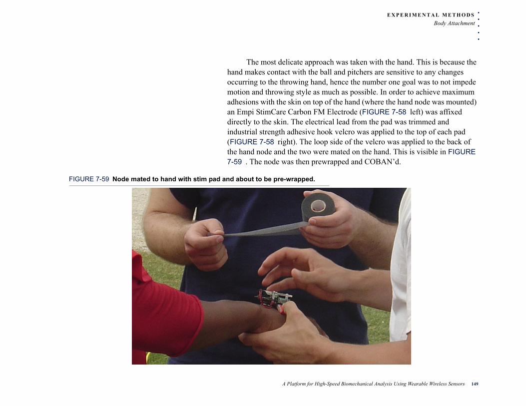
. . .
. .E X P E R I M E N T A L M E T H O D S
Body Attachment
The most delicate approach was taken with the hand. This is because the hand makes contact with the ball and pitchers are sensitive to any changes occurring to the throwing hand, hence the number one goal was to not impede motion and throwing style as much as possible. In order to achieve maximum adhesions with the skin on top of the hand (where the hand node was mounted) an Empi StimCare Carbon FM Electrode (FIGURE 7-58 left) was affixed directly to the skin. The electrical lead from the pad was trimmed and industrial strength adhesive hook velcro was applied to the top of each pad (FIGURE 7-58 right). The loop side of the velcro was applied to the back of the hand node and the two were mated on the hand. This is visible in FIGURE 7-59 . The node was then prewrapped and COBAN’d.
FIGURE 7-59 Node mated to hand with stim pad and about to be pre-wrapped.
A Platform for High-Speed Biomechanical Analysis Using Wearable Wireless Sensors 149
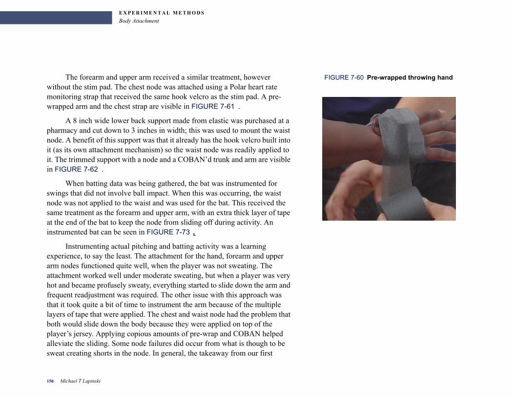
E X P E R I M E N T A L M E T H O D S
Body Attachment
FIGURE 7-60 Pre-wrapped throwing handThe forearm and upper arm received a similar treatment, however without the stim pad. The chest node was attached using a Polar heart rate monitoring strap that received the same hook velcro as the stim pad. A pre-wrapped arm and the chest strap are visible in FIGURE 7-61 .
A 8 inch wide lower back support made from elastic was purchased at a pharmacy and cut down to 3 inches in width; this was used to mount the waist node. A benefit of this support was that it already has the hook velcro built into it (as its own attachment mechanism) so the waist node was readily applied to it. The trimmed support with a node and a COBAN’d trunk and arm are visible in FIGURE 7-62 .
When batting data was being gathered, the bat was instrumented for swings that did not involve ball impact. When this was occurring, the waist node was not applied to the waist and was used for the bat. This received the same treatment as the forearm and upper arm, with an extra thick layer of tape at the end of the bat to keep the node from sliding off during activity. An instrumented bat can be seen in FIGURE 7-73 .
Instrumenting actual pitching and batting activity was a learning experience, to say the least. The attachment for the hand, forearm and upper arm nodes functioned quite well, when the player was not sweating. The attachment worked well under moderate sweating, but when a player was very hot and became profusely sweaty, everything started to slide down the arm and frequent readjustment was required. The other issue with this approach was that it took quite a bit of time to instrument the arm because of the multiple layers of tape that were applied. The chest and waist node had the problem that both would slide down the body because they were applied on top of the player’s jersey. Applying copious amounts of pre-wrap and COBAN helped alleviate the sliding. Some node failures did occur from what is though to be sweat creating shorts in the node. In general, the takeaway from our first
150 Michael T Lapinski
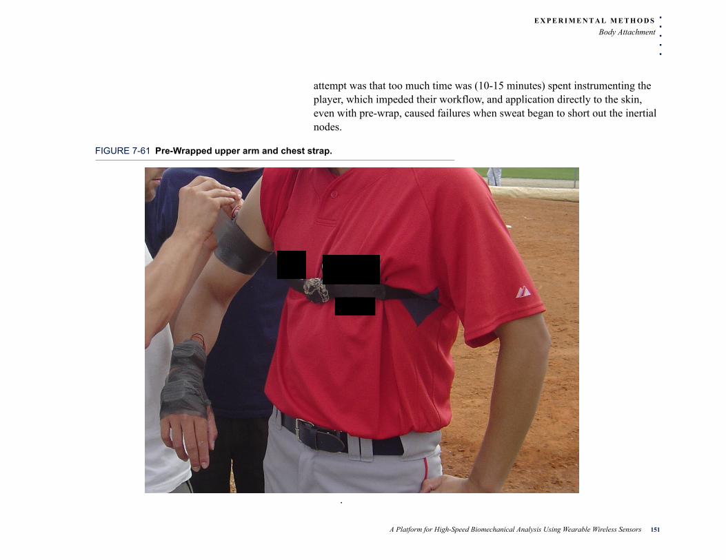
. . .
. .E X P E R I M E N T A L M E T H O D S
Body Attachment
attempt was that too much time was (10-15 minutes) spent instrumenting the player, which impeded their workflow, and application directly to the skin, even with pre-wrap, caused failures when sweat began to short out the inertial nodes.
FIGURE 7-61 Pre-Wrapped upper arm and chest strap.
.
A Platform for High-Speed Biomechanical Analysis Using Wearable Wireless Sensors 151
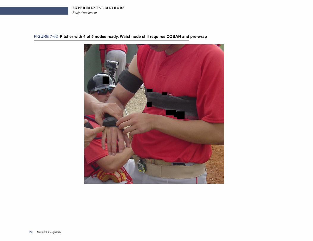
E X P E R I M E N T A L M E T H O D S
Body Attachment
FIGURE 7-62 Pitcher with 4 of 5 nodes ready. Waist node still requires COBAN and pre-wrap
152 Michael T Lapinski
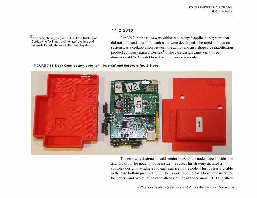
. . .
. .E X P E R I M E N T A L M E T H O D S
Body Attachment
7 .1 .2 201017A very big thank you goes out to Steve Buckley of
Corflex who facilitated and donated the time and materials to build the rapid attachment system.
For 2010, both issues were addressed. A rapid application system that did not slide and a case for each node were developed. The rapid application system was a collaboration between the author and an orthopedic rehabilitation product company named Corflex17. The case design came via a three dimensional CAD model based on node measurements.
FIGURE 7-63 Node Case (bottom case, left) (lid, right) and Hardware Rev 2 Node
The case was designed to add minimal size to the node placed inside of it and not allow the node to move inside the case. This strategy dictated a complex design that adhered to each surface of the node. This is clearly visible in the case bottom pictured in FIGURE 7-63 . The lid has a large protrusion for the battery and two relief holes to allow viewing of the on-node LED and allow
A Platform for High-Speed Biomechanical Analysis Using Wearable Wireless Sensors 153
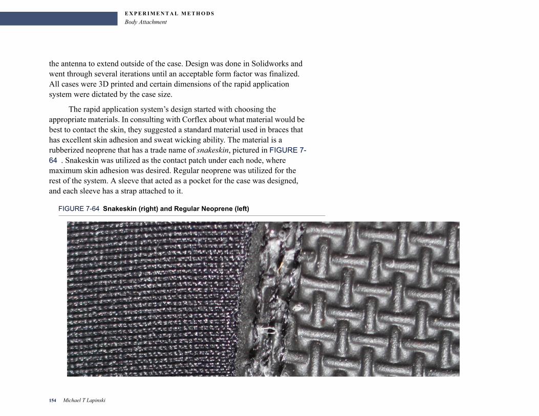
E X P E R I M E N T A L M E T H O D S
Body Attachment
the antenna to extend outside of the case. Design was done in Solidworks and went through several iterations until an acceptable form factor was finalized. All cases were 3D printed and certain dimensions of the rapid application system were dictated by the case size.
The rapid application system’s design started with choosing the appropriate materials. In consulting with Corflex about what material would be best to contact the skin, they suggested a standard material used in braces that has excellent skin adhesion and sweat wicking ability. The material is a rubberized neoprene that has a trade name of snakeskin, pictured in FIGURE 7-64 . Snakeskin was utilized as the contact patch under each node, where maximum skin adhesion was desired. Regular neoprene was utilized for the rest of the system. A sleeve that acted as a pocket for the case was designed, and each sleeve has a strap attached to it.
FIGURE 7-64 Snakeskin (right) and Regular Neoprene (left)
154 Michael T Lapinski
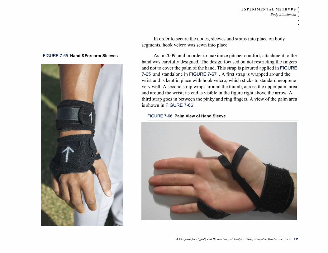
. . .
. .E X P E R I M E N T A L M E T H O D S
Body Attachment
In order to secure the nodes, sleeves and straps into place on body segments, hook velcro was sewn into place.
FIGURE 7-65 Hand &Forearm Sleeves As in 2009, and in order to maximize pitcher comfort, attachment to the hand was carefully designed. The design focused on not restricting the fingers and not to cover the palm of the hand. This strap is pictured applied in FIGURE 7-65 and standalone in FIGURE 7-67 . A first strap is wrapped around the wrist and is kept in place with hook velcro, which sticks to standard neoprene very well. A second strap wraps around the thumb, across the upper palm area and around the wrist; its end is visible in the figure right above the arrow. A third strap goes in between the pinky and ring fingers. A view of the palm area is shown in FIGURE 7-66 .
FIGURE 7-66 Palm View of Hand Sleeve
A Platform for High-Speed Biomechanical Analysis Using Wearable Wireless Sensors 155
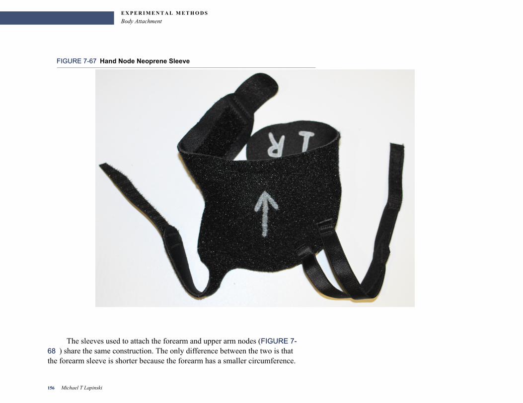
E X P E R I M E N T A L M E T H O D S
Body Attachment
FIGURE 7-67 Hand Node Neoprene Sleeve
The sleeves used to attach the forearm and upper arm nodes (FIGURE 7-68 ) share the same construction. The only difference between the two is that the forearm sleeve is shorter because the forearm has a smaller circumference.
156 Michael T Lapinski
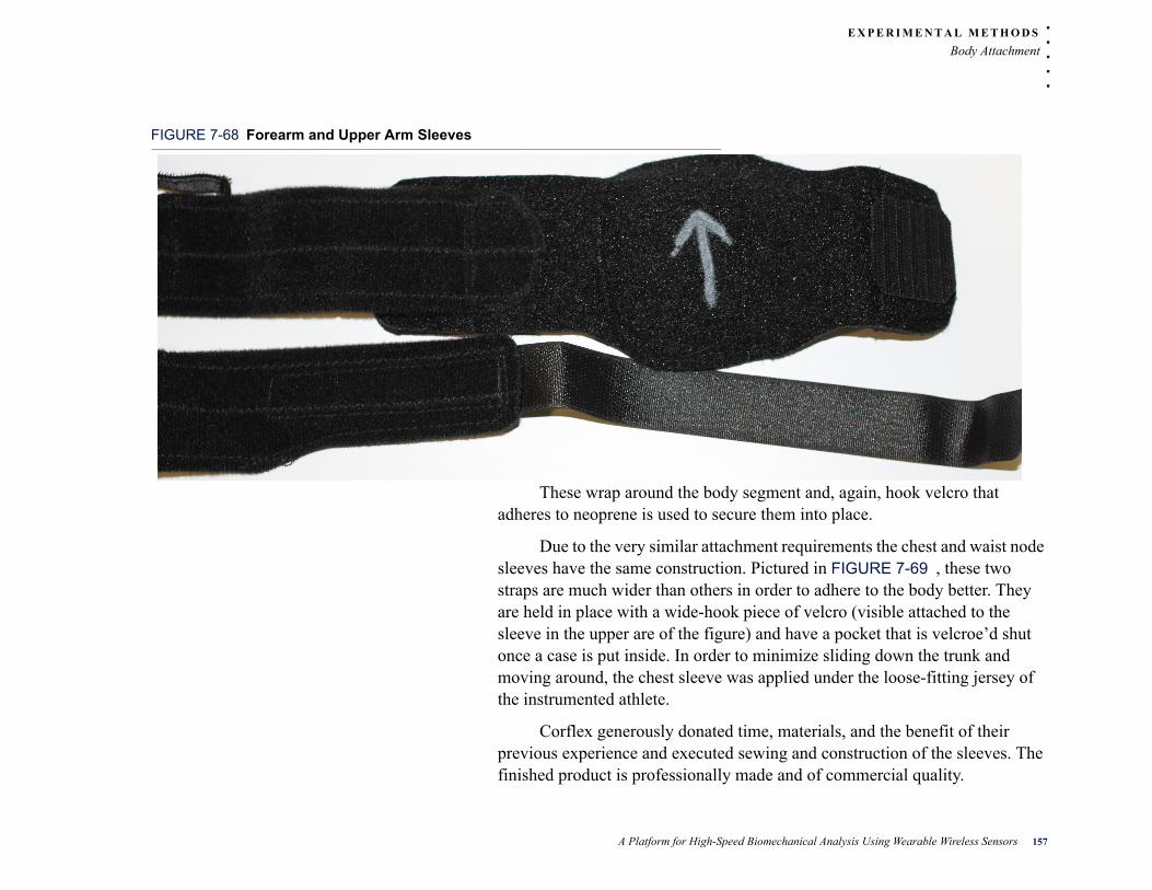
. . .
. .E X P E R I M E N T A L M E T H O D S
Body Attachment
FIGURE 7-68 Forearm and Upper Arm Sleeves
These wrap around the body segment and, again, hook velcro that adheres to neoprene is used to secure them into place.
Due to the very similar attachment requirements the chest and waist node sleeves have the same construction. Pictured in FIGURE 7-69 , these two straps are much wider than others in order to adhere to the body better. They are held in place with a wide-hook piece of velcro (visible attached to the sleeve in the upper are of the figure) and have a pocket that is velcroe’d shut once a case is put inside. In order to minimize sliding down the trunk and moving around, the chest sleeve was applied under the loose-fitting jersey of the instrumented athlete.
Corflex generously donated time, materials, and the benefit of their previous experience and executed sewing and construction of the sleeves. The finished product is professionally made and of commercial quality.
A Platform for High-Speed Biomechanical Analysis Using Wearable Wireless Sensors 157
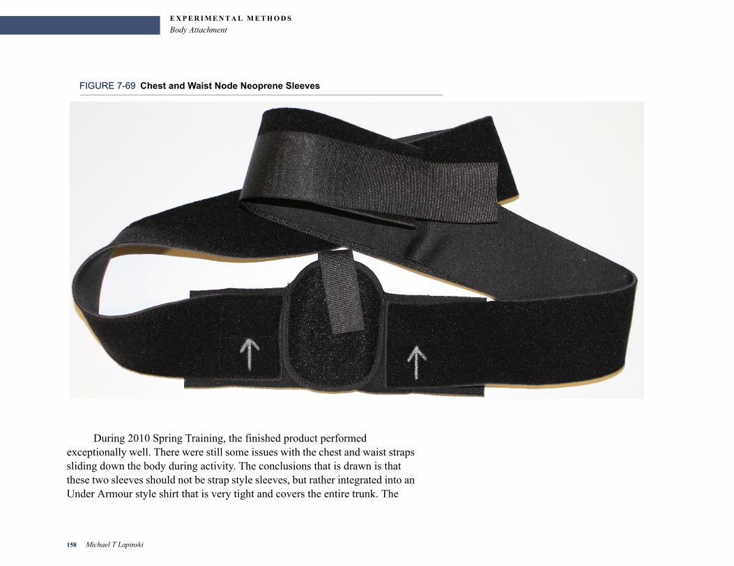
E X P E R I M E N T A L M E T H O D S
Body Attachment
FIGURE 7-69 Chest and Waist Node Neoprene Sleeves
During 2010 Spring Training, the finished product performed exceptionally well. There were still some issues with the chest and waist straps sliding down the body during activity. The conclusions that is drawn is that these two sleeves should not be strap style sleeves, but rather integrated into an Under Armour style shirt that is very tight and covers the entire trunk. The
158 Michael T Lapinski
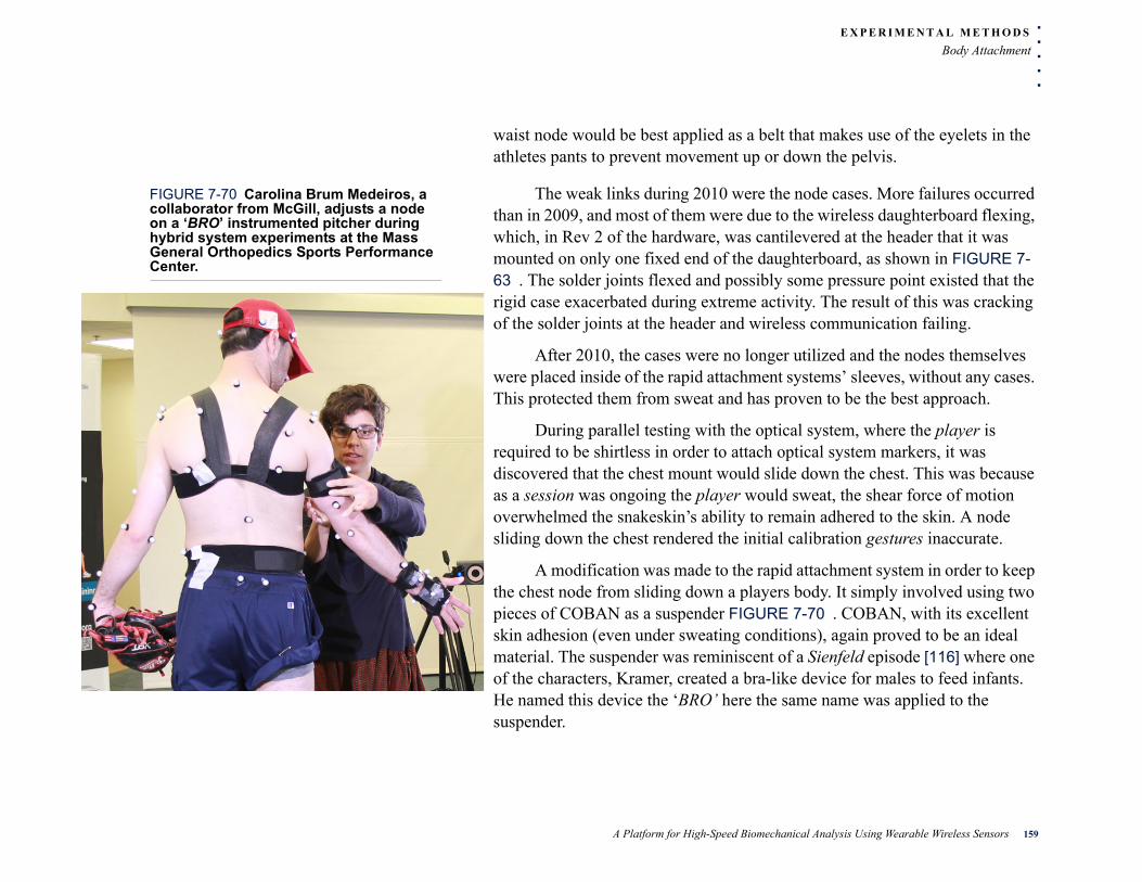
. . .
. .E X P E R I M E N T A L M E T H O D S
Body Attachment
waist node would be best applied as a belt that makes use of the eyelets in the athletes pants to prevent movement up or down the pelvis.
FIGURE 7-70 Carolina Brum Medeiros, a collaborator from McGill, adjusts a node on a ‘BRO’ instrumented pitcher during hybrid system experiments at the Mass General Orthopedics Sports Performance Center.
The weak links during 2010 were the node cases. More failures occurred than in 2009, and most of them were due to the wireless daughterboard flexing, which, in Rev 2 of the hardware, was cantilevered at the header that it was mounted on only one fixed end of the daughterboard, as shown in FIGURE 7-63 . The solder joints flexed and possibly some pressure point existed that the rigid case exacerbated during extreme activity. The result of this was cracking of the solder joints at the header and wireless communication failing.
After 2010, the cases were no longer utilized and the nodes themselves were placed inside of the rapid attachment systems’ sleeves, without any cases. This protected them from sweat and has proven to be the best approach.
During parallel testing with the optical system, where the player is required to be shirtless in order to attach optical system markers, it was discovered that the chest mount would slide down the chest. This was because as a session was ongoing the player would sweat, the shear force of motion overwhelmed the snakeskin’s ability to remain adhered to the skin. A node sliding down the chest rendered the initial calibration gestures inaccurate.
A modification was made to the rapid attachment system in order to keep the chest node from sliding down a players body. It simply involved using two pieces of COBAN as a suspender FIGURE 7-70 . COBAN, with its excellent skin adhesion (even under sweating conditions), again proved to be an ideal material. The suspender was reminiscent of a Sienfeld episode [116] where one of the characters, Kramer, created a bra-like device for males to feed infants. He named this device the ‘BRO’ here the same name was applied to the suspender.
A Platform for High-Speed Biomechanical Analysis Using Wearable Wireless Sensors 159
E X P E R I M E N T A L M E T H O D S
Pitching Protocol
. . . . . . . . . . . . . . . . . . . . . . . . . . . . . . . . . . . . . . . . . . . . . . . . . . . . . . . . . . .7 . 2 P I T C H I N G P R O T O C O L
The process for actually gathering data is purposely made to be as simple as possible to involve minimum setup time per player and keep a fast flow of subjects with minimum downtime. In general, an athlete is instrumented, measured and allowed to go about their normal activity.
The pitching protocol starts by instrumenting the athlete with the previously described neoprene sleeves. The next steps involve performing anthropometric measurements and logging pitch data as each ball is thrown. To facilitate this, a custom logbook was created. The logbook consists of a first page for recording the anthropometric and biometric data for each pitcher (FIGURE 7-71 ). The measurements recorded are described in the Player and Session sections in Chapter 3 (3.1.0.1 and 3.1.0.2).
Three types of calibration gestures are initially recorded for each session. The first of these involves the player standing upright, with both hands at their sides. The second involved the player standing in anatomic position. The third positioned the player with the arms abducted 90 degrees at the shoulder and the elbows at 90 degrees of flexion, forming a plane that is drawn by the shoulder, elbow and wrist joints. Each of these stances are recorded twice and the same calibration protocol is followed for pitchers and batters.
160 Michael T Lapinski
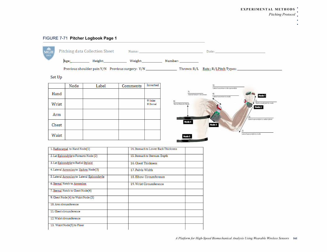
. . .
. .E X P E R I M E N T A L M E T H O D S
Pitching Protocol
FIGURE 7-71 Pitcher Logbook Page 1
A Platform for High-Speed Biomechanical Analysis Using Wearable Wireless Sensors 161

E X P E R I M E N T A L M E T H O D S
Pitching Protocol
FIGURE 7-72 Pitcher Logbook Pages 2-8
The following pages of the logbook are all identical; an example is presented in FIGURE 7-72 . These are used to record data for each pitch that is thrown. In order to effectively gather all necessary data, 3 people are required. One person is the system operator who monitors and controls the Network Control Application (Section 6.1). In continuous pitching mode, the operator is also broadcasting the Sequence Number (Section 6.1.5) to the data recorder and radar gun operator. For each pitch, the data recorder is responsible for
162 Michael T Lapinski
. . .
. .E X P E R I M E N T A L M E T H O D S
Batting Protocol
logging the File Name, Sequence Number, Pitch Type and Pitch Location. The radar gun operator is responsible for standing behind the catcher and recording the Sequence Number and the incoming pitch speed in miles per hour. If single gesture capture mode is used, there is no Sequence Number, so a filename is recorded for each pitch. Once the pitching Session concludes, the radar gun operator’s pitch speeds are rectified with the Sequence Numbers or File Names and added to the data recorders pitching sheet.
The next steps in the process involve using the Data Translation Application (Section 6.2) and the Data Processing and Import Application (Section 6.4) to process and load data into the data store. This processes are the same for pitching and batting. Optical system synchronization will be presented in Section 7.5.
. . . . . . . . . . . . . . . . . . . . . . . . . . . . . . . . . . . . . . . . . . . . . . . . . . . . . . . . . . .7 . 3 B A T T I N G P R O T O C O L
Batting experimentation consists of two different protocols. The first is a directed protocol, where the batter performs free swings with an instrumented bat, hits balls off of the tee with instruction on where the ball should go, then hits some soft toss pitches. The second fits more into the routine training activity of batting practice (BP) and the system runs in continuous mode.
7 .3 .1 D i rected Bat t ing Protocol
Historically, the directed batting took place in the batting cages at the minor league facilities of a major league baseball team, hence the title of the first page of the logbook (FIGURE 7-74 ) is Batting Cage Data Collection Sheet. The portability of a wearable inertial system does not prevent this from
A Platform for High-Speed Biomechanical Analysis Using Wearable Wireless Sensors 163
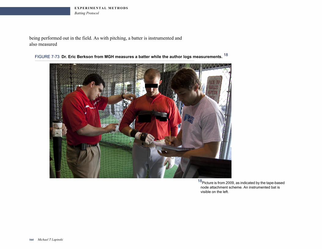
E X P E R I M E N T A L M E T H O D S
Batting Protocol
being performed out in the field. As with pitching, a batter is instrumented and also measured
FIGURE 7-73 Dr. Eric Berkson from MGH measures a batter while the author logs measurements. 18
18Picture is from 2009, as indicated by the tape-based node attachment scheme. An instrumented bat is visible on the left.
164 Michael T Lapinski
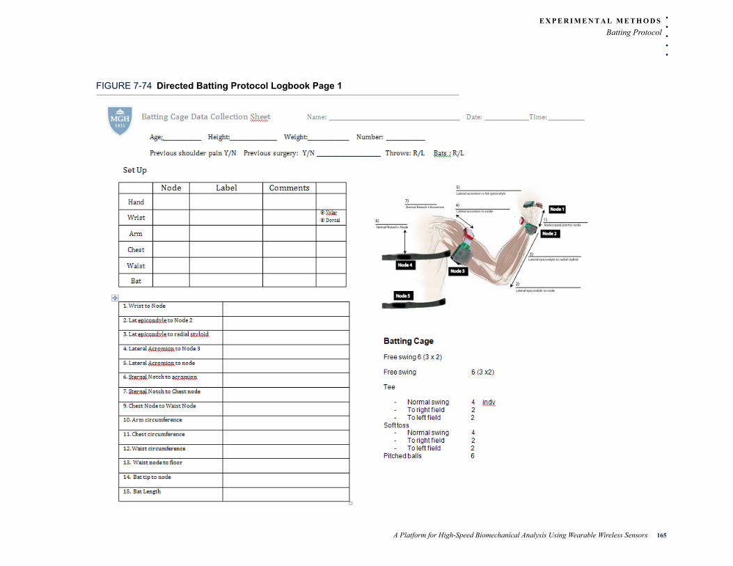
. . .
. .E X P E R I M E N T A L M E T H O D S
Batting Protocol
FIGURE 7-74 Directed Batting Protocol Logbook Page 1
A Platform for High-Speed Biomechanical Analysis Using Wearable Wireless Sensors 165

E X P E R I M E N T A L M E T H O D S
Batting Protocol
The directed protocol involves the batter performing a variety of gestures at the direction of the system operator. These gestures are:
With an instrumented bat at home plate:
• 6 x Free Swing - batter swinging the bat with no impact
With an un-instrumented bat hitting from a batting tee at home plate:
• 4 x Hit From Tee Straight - batter in instructed to hit the ball straight into center field
• 2 x Hit From Tee Right - batter is instructed to hit the ball into right field• 3 x Hit From Tee Left - batter is instructed to hit the ball into left field
With an un-instrumented bat from home plate and a pitcher throwing underhand from half the distance between the pitching mound and home plate:
• 4 x Hit Straight - batter is instructed to hit the ball straight into center field• 2 x Hit Right - batter is instructed to hit the ball into right field• 3 x Hit Left - batter is instructed to hit the ball into left field
With an un-instrumented bat from home plate and a pitcher throwing overhand at a moderate speed (40 - 65 MPH):
• 6 x Hit Ball
As these swings and hits are occurring, an operator is controlling the network and dictating File Names to the data recorder and radar gun operator. The data recorder logs File Name, Location of where the ball went on the field (via a graphic of the field on the sheet) and the trajectory arc of the ball when it was hit. The radar gun operator is recording the outgoing speed of the ball, and in the case of pitched balls the incoming pitch speed and the File Names.
166 Michael T Lapinski

. . .
. .E X P E R I M E N T A L M E T H O D S
Batting Protocol
FIGURE 7-75 Directed Batting Protocol Logbook Swing Annotation Page
A Platform for High-Speed Biomechanical Analysis Using Wearable Wireless Sensors 167

E X P E R I M E N T A L M E T H O D S
Batting Protocol
7 .3 .2 Bat t ing Pract ice Protocol
Batting practice, or BP as it is called by those in the know, involves a continuous series of moderate speed (45 - 75MPH) overhead pitches thrown by a professional pitcher from halfway between home plate and the pitching mound. This scenario is ideal for utilizing the system’s Continuous Sampling Mode (Section 6.1.5).
The protocol followed for BP is the same as pitching in continuous mode, with the caveat that pitch data is not logged. The data logged is the same data as is logged with directed batting during overhead soft toss.
168 Michael T Lapinski
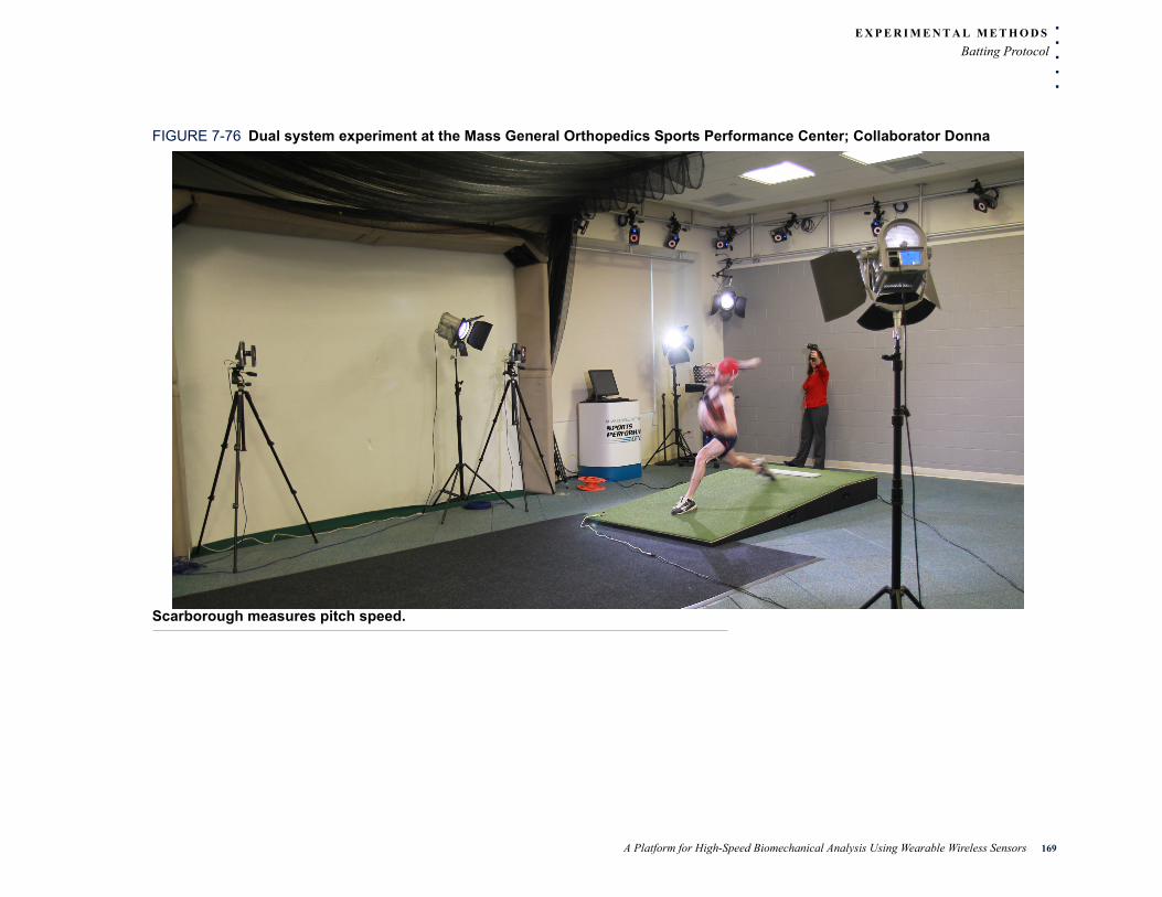
. . .
. .E X P E R I M E N T A L M E T H O D S
Batting Protocol
FIGURE 7-76 Dual system experiment at the Mass General Orthopedics Sports Performance Center; Collaborator Donna
Scarborough measures pitch speed.
A Platform for High-Speed Biomechanical Analysis Using Wearable Wireless Sensors 169
E X P E R I M E N T A L M E T H O D S
Dual System Experiments
. . . . . . . . . . . . . . . . . . . . . . . . . . . . . . . . . . . . . . . . . . . . . . . . . . . . . . . . . . .7 . 4 D U A L S Y S T E M E X P E R I M E N T S
Gathering data from both an inertial and optical system simultaneously for the purposes of comparing the two requires instrumentation of the player with inertial nodes as well as optical markers (FIGURE 7-76 ) and synchronization of data streams from both systems. The synchronization system, which spans the hardware, firmware and software sections of this dissertation, is described in Sections 4.3.1, 5.1.1, 6.1.8.
The activity performed during dual system experiments is only pitching, and the protocol followed is that of non-continuous pitching. Additionally, the protocol follows the sequence of starting and stopping the recording of both systems, as described in the optical system synchronization timing diagram (FIGURE 5-41 ). Two additional pieces of data are gathered for each gesture: the optical system framerate and the offset delta between the start times of both systems. Both of these are utilized during gesture annotation (Section 6.4.4.2).
7 . 5 D A T A T R A N S L A T I O N A N D
. . . . . . . . . . . . . . . . . . . . . . . . . . . . . . . . . . . . . . . . . . . . . . . . . . . . . . . . . . .A N N O T A T I O N
The underlying mechanics of how data moves from sensors via communication busses to a microcontroller and finally to µSD cards on the nodes attached to body segments has been described in Chapters 4, 5 and 6. The data translation operator interface, used to retrieves data from the µSD cards, is described Section 6.2.
170 Michael T Lapinski
. . .
. .E X P E R I M E N T A L M E T H O D S
Data Translation and Annotation
Once a given data gathering protocol has been executed, the process for translating data is followed. The data is available in flat comma-separated-value format files for processing by the Data Processing and Annotation Application (Section 6.4). This application parses the files, applies calibration offsets and inserts all of this data into the database using the bulk import (Section 6.4.4.1) feature of the application. The final step is to use the data that is logged during each Session and annotate each of the Gestures to enable classification, data mining and analysis of the data.
The precursor to annotating gesture data is to create a Player and Session for that player. Some of the anthropomorphic and all of the biometric data, recorded on Page 1 in both logbooks, is used in conjunction with the Player Info Tab (Section 6.4.2) to create the Player. Some of the anthropometric data and node body segment location data, from the same logbook page, are used to create a new Session using the Player Sessions Tab (Section FIGURE 6-53 ).
The annotation process involves matching gesture filenames with those that are recorded in the logbook and, depending on the gesture type, the proper parameters are entered in the Player Gesture Tab (FIGURE 6-55 ) that is part of the Data Processing and Annotation Application (Section 6.4).
A Platform for High-Speed Biomechanical Analysis Using Wearable Wireless Sensors 171
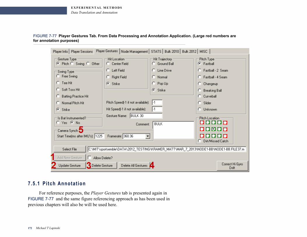
E X P E R I M E N T A L M E T H O D S
Data Translation and Annotation
FIGURE 7-77 Player Gestures Tab. From Data Processing and Annotation Application. (Large red numbers are for annotation purposes)
7 .5 .1 P i tch Annotat ion
For reference purposes, the Player Gestures tab is presented again in FIGURE 7-77 and the same figure referencing approach as has been used in previous chapters will also be will be used here.
172 Michael T Lapinski

. . .
. .E X P E R I M E N T A L M E T H O D S
Data Translation and Annotation
The first step involves the operator selecting the pitch that has been matched to the filename in the Player Gestures list (6-33-10). Annotating a pitch requires translating data from the pitching logbook to the various radio button groups in the Player Gestures Tab.
The groups relevant to a pitch are:
• Gesture Type - This is always Pitch• Pitch Type - taken from logbook’s Pitch Type column and based on the pitch type
signaled by the pitcher while throwing.• Pitch Speed (Text Field) - measured via radar and taken from the logbook’s Pitch
Speed column and entered in the Pitch Speed text area. • Pitch Location - taken from the logbook’s Pitch Location column and entered in
the Pitch Location radio group.
Once the correct radio groups are selected, the operator clicks the Update Gesture button and annotation has been completed.
7 .5 .2 Swing Annotat ion
Annotation a swing also starts with the operator selecting a filename matched gesture in the Player Gestures list (6-33-10) and translating logbook data to the appropriate radio button groups and text fields in the Player Gestures tab, FIGURE 7-77 .
The groups relevant to a swing are:
• Gesture Type - This is always Swing• Swing Type - taken from logbook Activity column for directed batting; there are
also options for swings during BP and at off-mound pitches.• Pitch Speed (Text Field) - measured by radar, recorded in the Pitch Speed column
and entered in the Pitch Speed text area; this is incoming pitch speed. • Hit Speed (Text Field) - Also measured by radar and logged as outgoing hit speed.
Data is entered into the Hit Speed text field. • Hit Location - where the ball went, if it was struck. If not, the swing is recorded as
a strike.
A Platform for High-Speed Biomechanical Analysis Using Wearable Wireless Sensors 173

E X P E R I M E N T A L M E T H O D S
Data Translation and Annotation
• Hit Trajectory - the arc that the ball flew in if stuck or a strike if the ball was not struck.
• Bat Instrumentation - For Free Swings, the bat is instrumented and the Yes radio button is chosen, otherwise No.
Once the correct radio groups are selected the operator clicks the Update Gesture button and annotation has been completed.
7 .5 .3 Dual System Annotat ion
When a dual system experiment, using the inertial and optical system in parallel, is performed two pieces of additional data are logged: synchronization offset and framerate. These are entered into the Camera Synch area of the Player Gestures tab. The remaining annotation process follows the same procedure as described in the previous two sections.
174 Michael T Lapinski
. . .
. .VA L I D A T I O N A N D E R R O R S O U R C E S
VALIDATION AND
. . . .
. . . . . . . . . . . . . . . . . . . . . . . . . . . . . . . . . . . . . .ERROR SOURCES
-
This chapter seeks to answer one question, “How good are we?”, mainly by presenting measurement techniques. A validation methodology is developed and results are presented that compare the inertial system to an established optical one. But first, an examination of the sources and quantification of error that are present using an inertial approach is given.
A Platform for High-Speed Biomechanical Analysis Using Wearable Wireless Sensors 175
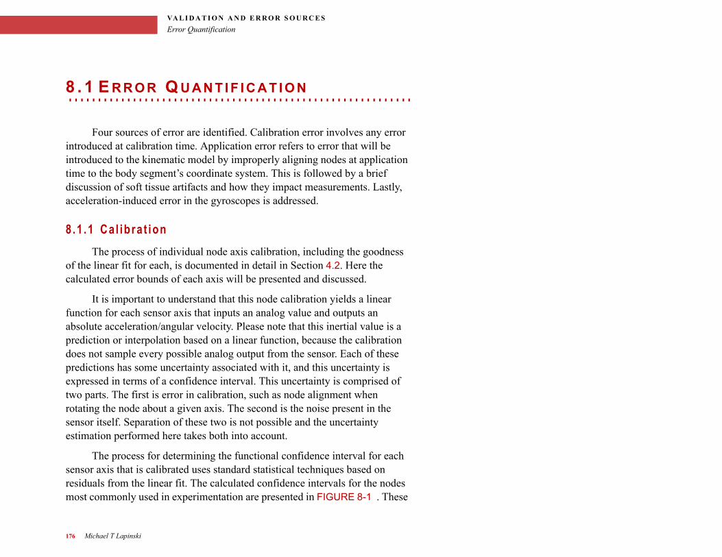
VA L I D A T I O N A N D E R R O R S O U R C E S
Error Quantification
. . . . . . . . . . . . . . . . . . . . . . . . . . . . . . . . . . . . . . . . . . . . . . . . . . . . . . . . . . .8 . 1 E R R O R Q U A N T I F I C A T I O N
Four sources of error are identified. Calibration error involves any error introduced at calibration time. Application error refers to error that will be introduced to the kinematic model by improperly aligning nodes at application time to the body segment’s coordinate system. This is followed by a brief discussion of soft tissue artifacts and how they impact measurements. Lastly, acceleration-induced error in the gyroscopes is addressed.
8 .1 .1 Ca l ibra t ion
The process of individual node axis calibration, including the goodness of the linear fit for each, is documented in detail in Section 4.2. Here the calculated error bounds of each axis will be presented and discussed.
It is important to understand that this node calibration yields a linear function for each sensor axis that inputs an analog value and outputs an absolute acceleration/angular velocity. Please note that this inertial value is a prediction or interpolation based on a linear function, because the calibration does not sample every possible analog output from the sensor. Each of these predictions has some uncertainty associated with it, and this uncertainty is expressed in terms of a confidence interval. This uncertainty is comprised of two parts. The first is error in calibration, such as node alignment when rotating the node about a given axis. The second is the noise present in the sensor itself. Separation of these two is not possible and the uncertainty estimation performed here takes both into account.
The process for determining the functional confidence interval for each sensor axis that is calibrated uses standard statistical techniques based on residuals from the linear fit. The calculated confidence intervals for the nodes most commonly used in experimentation are presented in FIGURE 8-1 . These
176 Michael T Lapinski
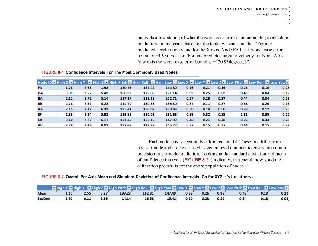
. . .
. .VA L I D A T I O N A N D E R R O R S O U R C E S
Error Quantification
intervals allow stating of what the worst-case error is in our analog to absolute prediction. In lay terms, based on the table, we can state that “For any predicted acceleration value for the X axis, Node FA has a worse case error bound of ±1.93m/s2.” or “For any predicted angular velocity for Node AA’s Yaw axis the worst case error bound is ±120.93degrees/s”.
FIGURE 8-1 Confidence Intervals For The Most Commonly Used Nodes
Each node axis is separately calibrated and fit. These fits differ from node-to-node and are never used as generalized numbers to ensure maximum precision in per-node prediction. Looking at the standard deviation and mean of confidence intervals (FIGURE 8-2 ) indicates, in general, how good the calibration process is for the entire population of nodes.
FIGURE 8-2 Overall Per Axis Mean and Standard Deviation of Confidence Intervals (Gs for XYZ, °/s for others)
A Platform for High-Speed Biomechanical Analysis Using Wearable Wireless Sensors 177
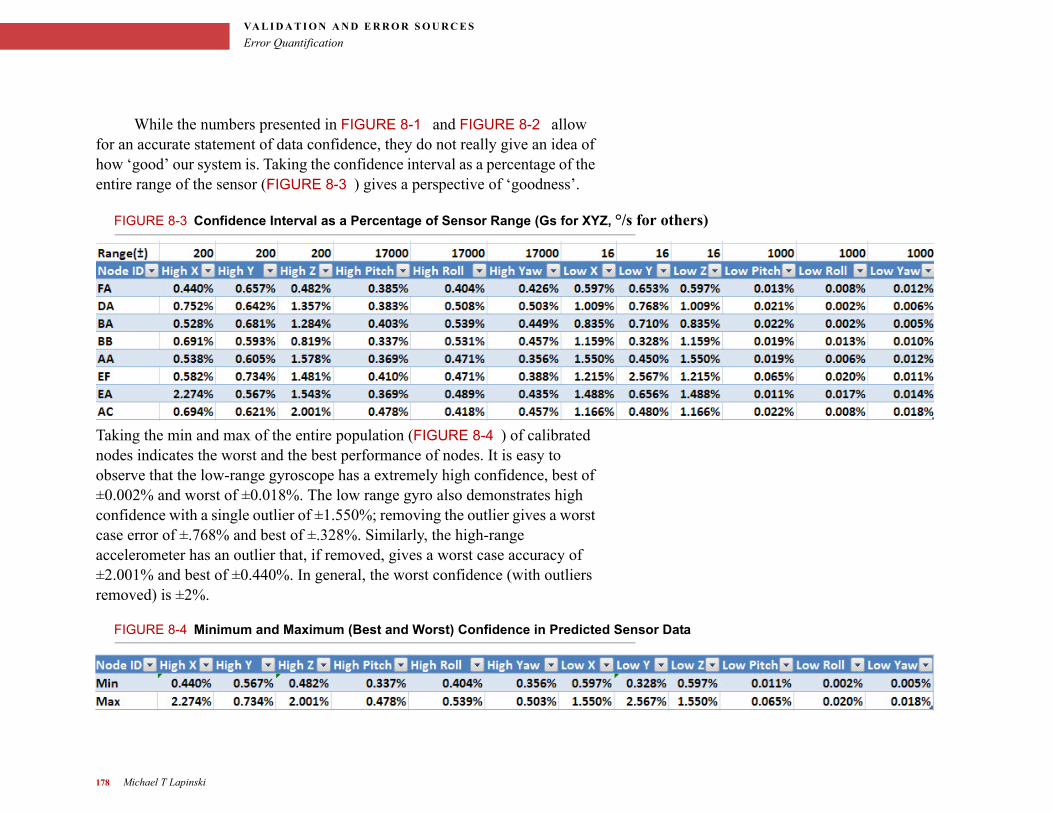
VA L I D A T I O N A N D E R R O R S O U R C E S
Error Quantification
While the numbers presented in FIGURE 8-1 and FIGURE 8-2 allow for an accurate statement of data confidence, they do not really give an idea of how ‘good’ our system is. Taking the confidence interval as a percentage of the entire range of the sensor (FIGURE 8-3 ) gives a perspective of ‘goodness’.
FIGURE 8-3 Confidence Interval as a Percentage of Sensor Range (Gs for XYZ, °/s for others)
Taking the min and max of the entire population (FIGURE 8-4 ) of calibrated nodes indicates the worst and the best performance of nodes. It is easy to observe that the low-range gyroscope has a extremely high confidence, best of ±0.002% and worst of ±0.018%. The low range gyro also demonstrates high confidence with a single outlier of ±1.550%; removing the outlier gives a worst case error of ±.768% and best of ±.328%. Similarly, the high-range accelerometer has an outlier that, if removed, gives a worst case accuracy of ±2.001% and best of ±0.440%. In general, the worst confidence (with outliers removed) is ±2%.
FIGURE 8-4 Minimum and Maximum (Best and Worst) Confidence in Predicted Sensor Data
178 Michael T Lapinski

. . .
. .VA L I D A T I O N A N D E R R O R S O U R C E S
Error Quantification
8 .1 .2 Appl ica t ion (Coord inate System Misa l ignment )
When performing an inertial to optical system comparison, an important assumption is made. That the coordinate systems of each segment (or limb that a node is attached to) in each system are aligned. This alignment is crucial for comparing segment orientations of both systems. Error in the alignment occurs when the inertial nodes are applied to an athlete’s body. The sources of the error are due to varying body types and physical dimensions of athletes and difficulty in perfectly aligning the axes of the inertial node to skeletal landmarks.
The hand and forearm nodes do not suffer from a great deal of misalignment because both are placed on relatively flat surfaces on those segments. These surfaces happen to align very well with the planes that are used to define optical system coordinate systems.
For the upper arm, which is modeled as a cone and in reality has a cylindrical shape without flat surfaces, it is more difficult to ascertain the exact coordinate system orientation and apply the node accordingly. The Z-Axis is easy, as it runs along the humerus, and the X-axis is more difficult, as it is defined by the line drawn form the medial to lateral epicondyle. At application time, a best effort is made to align these axes, however this alignment is not perfect.
Measuring the alignment error on all three axes requires a common global coordinate system between both systems. Otherwise, it is only possible to measure the error about the X and Y axes. The two-axis approach is possible by considering that any global coordinate system has the plane defined by the X and Y axes orthogonal to gravity (if the floor defining the coordinate system is flat). By nature, the accelerometer measurement of the nodes is also orthogonal to Earth’s gravity vector. Therefore, a calculated tilt and roll of an inertial node relative to gravity (given by the projection of Earth’s 1G Gravitational field onto the three accelerometer axes) when the node is not
A Platform for High-Speed Biomechanical Analysis Using Wearable Wireless Sensors 179
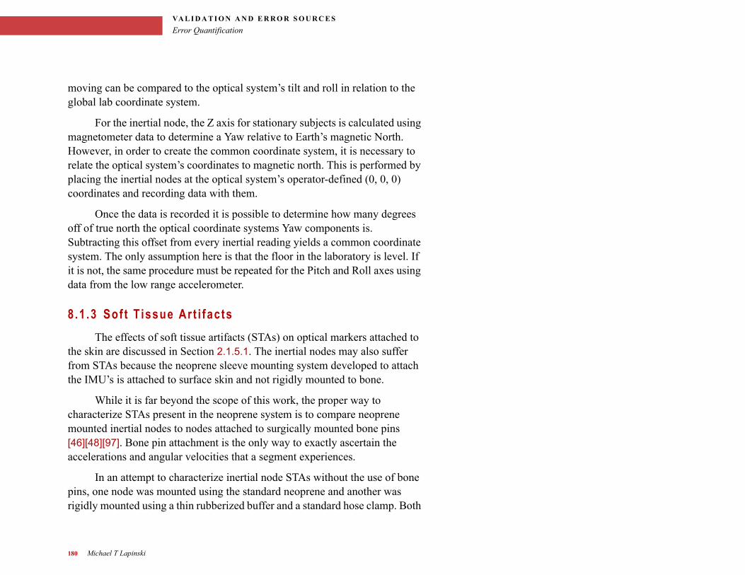
VA L I D A T I O N A N D E R R O R S O U R C E S
Error Quantification
moving can be compared to the optical system’s tilt and roll in relation to the global lab coordinate system.
For the inertial node, the Z axis for stationary subjects is calculated using magnetometer data to determine a Yaw relative to Earth’s magnetic North. However, in order to create the common coordinate system, it is necessary to relate the optical system’s coordinates to magnetic north. This is performed by placing the inertial nodes at the optical system’s operator-defined (0, 0, 0) coordinates and recording data with them.
Once the data is recorded it is possible to determine how many degrees off of true north the optical coordinate systems Yaw components is. Subtracting this offset from every inertial reading yields a common coordinate system. The only assumption here is that the floor in the laboratory is level. If it is not, the same procedure must be repeated for the Pitch and Roll axes using data from the low range accelerometer.
8 .1 .3 Sof t T issue Ar t i fac ts
The effects of soft tissue artifacts (STAs) on optical markers attached to the skin are discussed in Section 2.1.5.1. The inertial nodes may also suffer from STAs because the neoprene sleeve mounting system developed to attach the IMU’s is attached to surface skin and not rigidly mounted to bone.
While it is far beyond the scope of this work, the proper way to characterize STAs present in the neoprene system is to compare neoprene mounted inertial nodes to nodes attached to surgically mounted bone pins [46][48][97]. Bone pin attachment is the only way to exactly ascertain the accelerations and angular velocities that a segment experiences.
In an attempt to characterize inertial node STAs without the use of bone pins, one node was mounted using the standard neoprene and another was rigidly mounted using a thin rubberized buffer and a standard hose clamp. Both
180 Michael T Lapinski
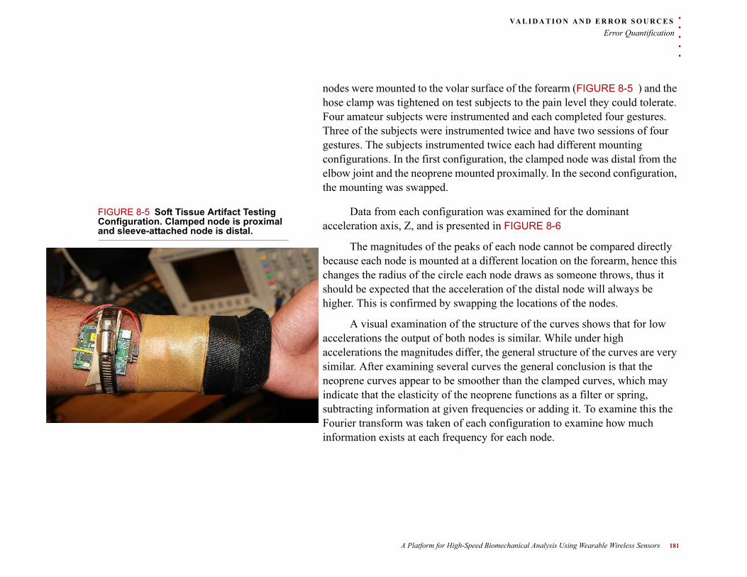
. . .
. .VA L I D A T I O N A N D E R R O R S O U R C E S
Error Quantification
nodes were mounted to the volar surface of the forearm (FIGURE 8-5 ) and the hose clamp was tightened on test subjects to the pain level they could tolerate. Four amateur subjects were instrumented and each completed four gestures. Three of the subjects were instrumented twice and have two sessions of four gestures. The subjects instrumented twice each had different mounting configurations. In the first configuration, the clamped node was distal from the elbow joint and the neoprene mounted proximally. In the second configuration, the mounting was swapped.
FIGURE 8-5 Soft Tissue Artifact Testing Configuration. Clamped node is proximal and sleeve-attached node is distal.
Data from each configuration was examined for the dominant acceleration axis, Z, and is presented in FIGURE 8-6
The magnitudes of the peaks of each node cannot be compared directly because each node is mounted at a different location on the forearm, hence this changes the radius of the circle each node draws as someone throws, thus it should be expected that the acceleration of the distal node will always be higher. This is confirmed by swapping the locations of the nodes.
A visual examination of the structure of the curves shows that for low accelerations the output of both nodes is similar. While under high accelerations the magnitudes differ, the general structure of the curves are very similar. After examining several curves the general conclusion is that the neoprene curves appear to be smoother than the clamped curves, which may indicate that the elasticity of the neoprene functions as a filter or spring, subtracting information at given frequencies or adding it. To examine this the Fourier transform was taken of each configuration to examine how much information exists at each frequency for each node.
A Platform for High-Speed Biomechanical Analysis Using Wearable Wireless Sensors 181
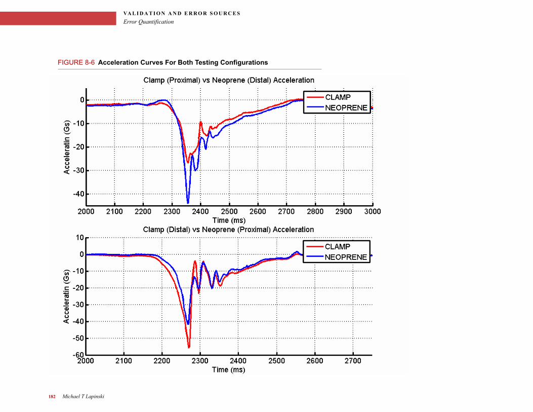
VA L I D A T I O N A N D E R R O R S O U R C E S
Error Quantification
FIGURE 8-6 Acceleration Curves For Both Testing Configurations
182 Michael T Lapinski
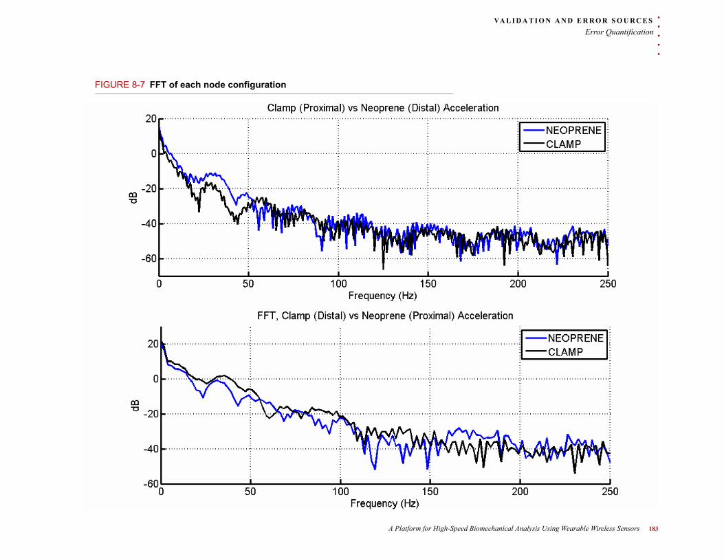
. . .
. .VA L I D A T I O N A N D E R R O R S O U R C E S
Error Quantification
FIGURE 8-7 FFT of each node configuration
A Platform for High-Speed Biomechanical Analysis Using Wearable Wireless Sensors 183
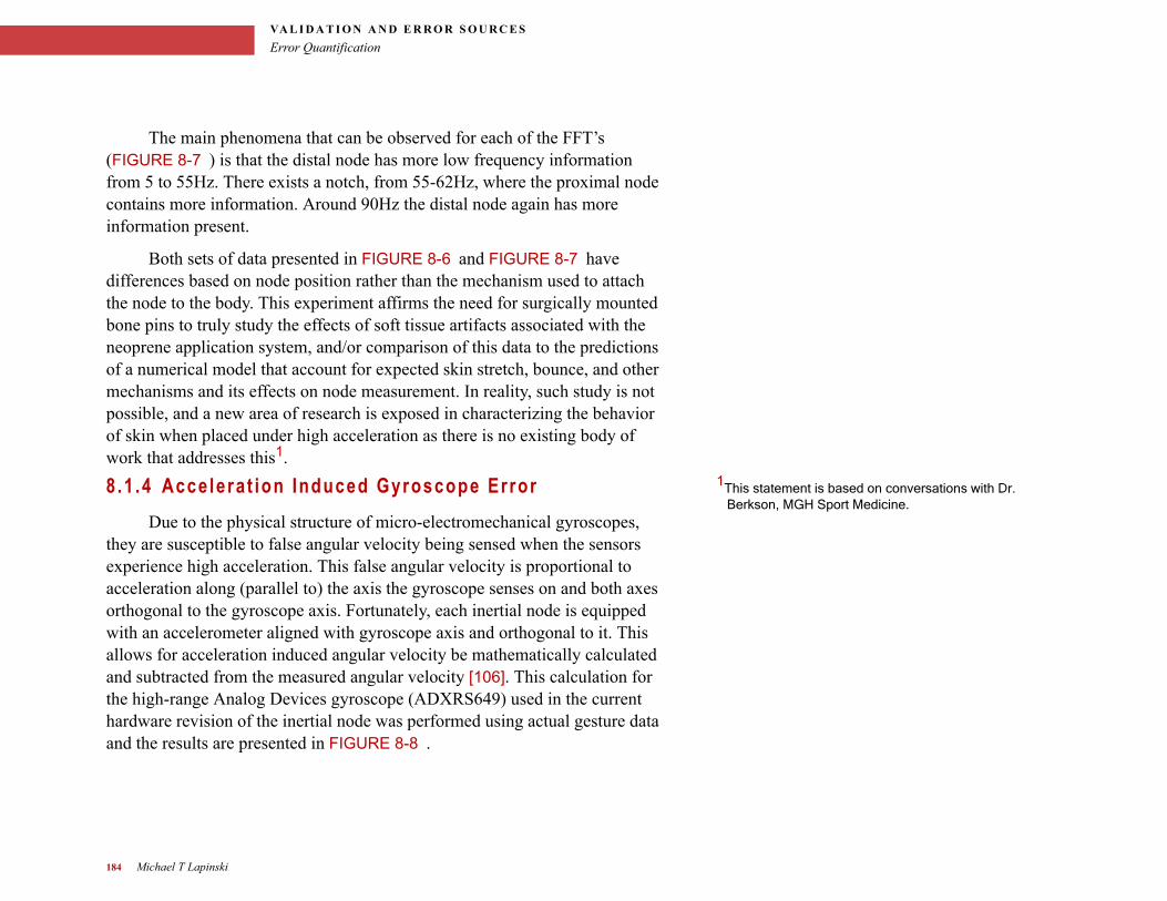
VA L I D A T I O N A N D E R R O R S O U R C E S
Error Quantification
The main phenomena that can be observed for each of the FFT’s (FIGURE 8-7 ) is that the distal node has more low frequency information from 5 to 55Hz. There exists a notch, from 55-62Hz, where the proximal node contains more information. Around 90Hz the distal node again has more information present.
Both sets of data presented in FIGURE 8-6 and FIGURE 8-7 have differences based on node position rather than the mechanism used to attach the node to the body. This experiment affirms the need for surgically mounted bone pins to truly study the effects of soft tissue artifacts associated with the neoprene application system, and/or comparison of this data to the predictions of a numerical model that account for expected skin stretch, bounce, and other mechanisms and its effects on node measurement. In reality, such study is not possible, and a new area of research is exposed in characterizing the behavior of skin when placed under high acceleration as there is no existing body of work that addresses this1.
1This statement is based on conversations with Dr. Berkson, MGH Sport Medicine.
8 .1 .4 Acce lera t ion Induced Gyroscope Error
Due to the physical structure of micro-electromechanical gyroscopes, they are susceptible to false angular velocity being sensed when the sensors experience high acceleration. This false angular velocity is proportional to acceleration along (parallel to) the axis the gyroscope senses on and both axes orthogonal to the gyroscope axis. Fortunately, each inertial node is equipped with an accelerometer aligned with gyroscope axis and orthogonal to it. This allows for acceleration induced angular velocity be mathematically calculated and subtracted from the measured angular velocity [106]. This calculation for the high-range Analog Devices gyroscope (ADXRS649) used in the current hardware revision of the inertial node was performed using actual gesture data and the results are presented in FIGURE 8-8 .
184 Michael T Lapinski
. . .
. .VA L I D A T I O N A N D E R R O R S O U R C E S
Error Quantification
FIGURE 8-8 Acceleration Induced Error Sample Data
A Platform for High-Speed Biomechanical Analysis Using Wearable Wireless Sensors 185
VA L I D A T I O N A N D E R R O R S O U R C E S
System Validation
The ADXRS649 is a newer part and is used in the latest revision of the inertial node, thus its is the focus of analysis here. A peak angular velocity of around 7,000 degrees/sec is seen at this gesture, and the parallel axis false angular velocity is less than 135 degrees/sec. At the same angular velocity, the acceleration at the orthogonal axes adds less than 8 degrees/sec of false angular velocity. This is gives a total of 143 degrees/sec of false angular velocity which is 1.8%, if data is left uncorrected. However, because the error can be calculated and all parameters necessary to do so are readily available we accommodate this in our analysis, and this phenomena does not present a source of system error.
. . . . . . . . . . . . . . . . . . . . . . . . . . . . . . . . . . . . . . . . . . . . . . . . . . . . . . . . . . .8 . 2 S Y S T E M V A L I D A T I O N
Comparison of the inertial system against the optical is another indication as to how ‘good’ the inertial system is. However, a tricky question arises when this comparison is performed: What if, for certain parameters, the inertial system is better than the optical?
Optical systems directly observe segment position and orientations via marker positions, and because of this they are better at providing these parameters. Their accuracy and precision is discussed in Section 2.1.5 in detail. Because of this, the kinematic calculations of the inertial system must use the optical as a ‘gold standard’ ground truth. When inertial parameters are considered, it is necessary to answer the above question. If the inertial system is better, then it is necessary to compare the optical system to the inertial and examine how ‘good’ it is at estimating inertial parameters and use the inertial system as the ‘gold standard’.
186 Michael T Lapinski
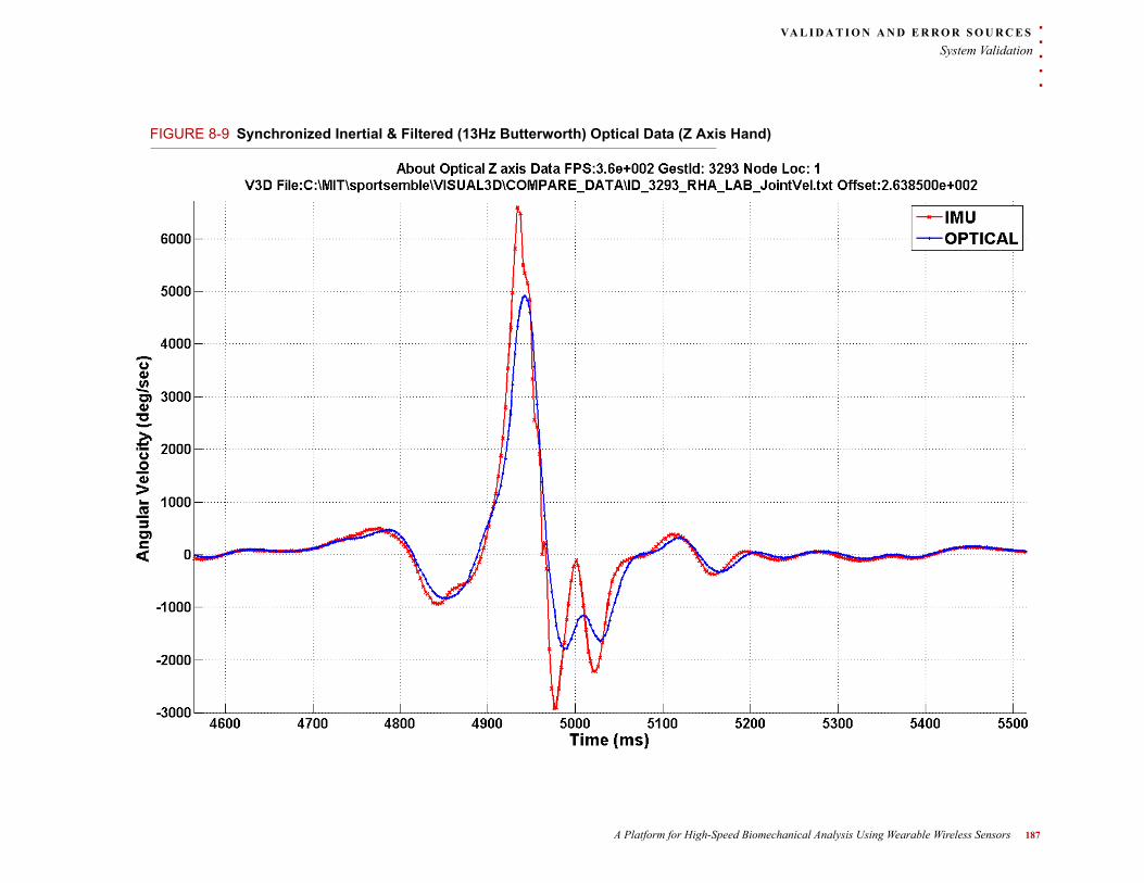
. . .
. .VA L I D A T I O N A N D E R R O R S O U R C E S
System Validation
FIGURE 8-9 Synchronized Inertial & Filtered (13Hz Butterworth) Optical Data (Z Axis Hand)
A Platform for High-Speed Biomechanical Analysis Using Wearable Wireless Sensors 187
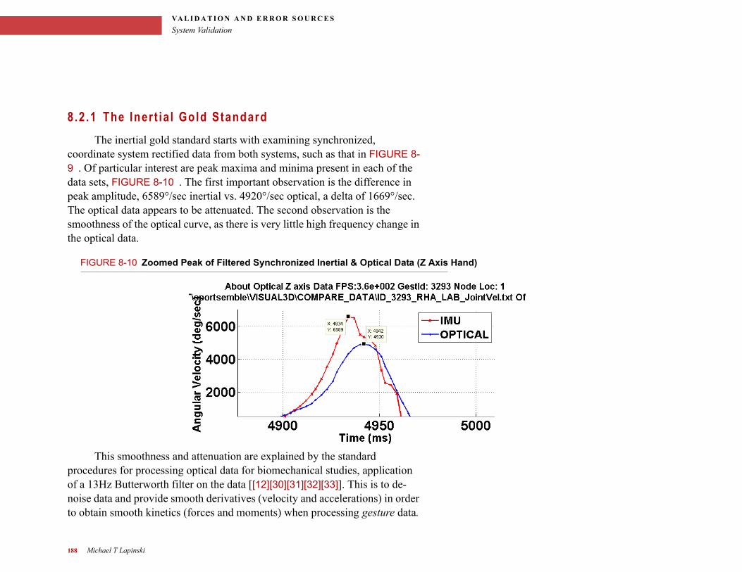
VA L I D A T I O N A N D E R R O R S O U R C E S
System Validation
8 .2 .1 The Iner t ia l Gold Standard
The inertial gold standard starts with examining synchronized, coordinate system rectified data from both systems, such as that in FIGURE 8-9 . Of particular interest are peak maxima and minima present in each of the data sets, FIGURE 8-10 . The first important observation is the difference in peak amplitude, 6589°/sec inertial vs. 4920°/sec optical, a delta of 1669°/sec. The optical data appears to be attenuated. The second observation is the smoothness of the optical curve, as there is very little high frequency change in the optical data.
FIGURE 8-10 Zoomed Peak of Filtered Synchronized Inertial & Optical Data (Z Axis Hand)
This smoothness and attenuation are explained by the standard procedures for processing optical data for biomechanical studies, application of a 13Hz Butterworth filter on the data [[12][30][31][32][33]]. This is to de-noise data and provide smooth derivatives (velocity and accelerations) in order to obtain smooth kinetics (forces and moments) when processing gesture data.
188 Michael T Lapinski

. . .
. .VA L I D A T I O N A N D E R R O R S O U R C E S
System Validation
Logically, the next step is to not filter the optical data and compare the two datasets again. The expected result is that the amplitude of the signal will not be attenuated at the cost of additional noise. Unfiltered data is presented in FIGURE 8-11 and the hypothesis holds true.
A Platform for High-Speed Biomechanical Analysis Using Wearable Wireless Sensors 189
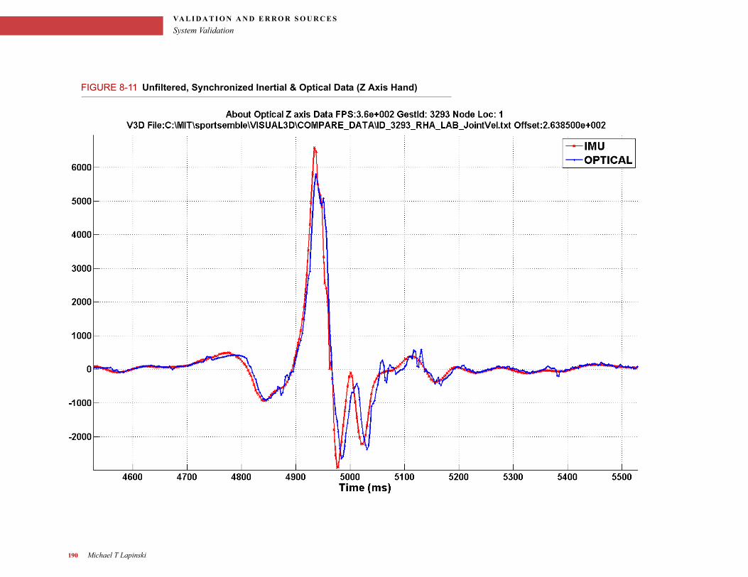
VA L I D A T I O N A N D E R R O R S O U R C E S
System Validation
FIGURE 8-11 Unfiltered, Synchronized Inertial & Optical Data (Z Axis Hand)
190 Michael T Lapinski
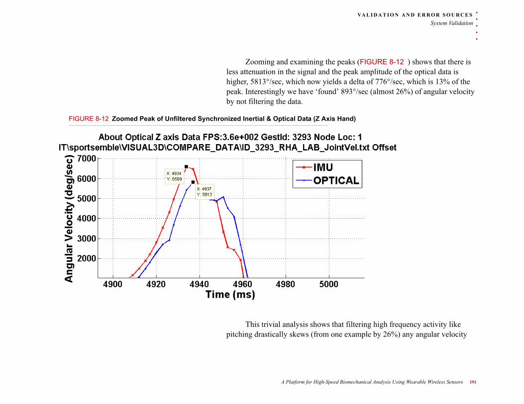
. . .
. .VA L I D A T I O N A N D E R R O R S O U R C E S
System Validation
Zooming and examining the peaks (FIGURE 8-12 ) shows that there is less attenuation in the signal and the peak amplitude of the optical data is higher, 5813°/sec, which now yields a delta of 776°/sec, which is 13% of the peak. Interestingly we have ‘found’ 893°/sec (almost 26%) of angular velocity by not filtering the data.
FIGURE 8-12 Zoomed Peak of Unfiltered Synchronized Inertial & Optical Data (Z Axis Hand)
This trivial analysis shows that filtering high frequency activity like pitching drastically skews (from one example by 26%) any angular velocity
A Platform for High-Speed Biomechanical Analysis Using Wearable Wireless Sensors 191
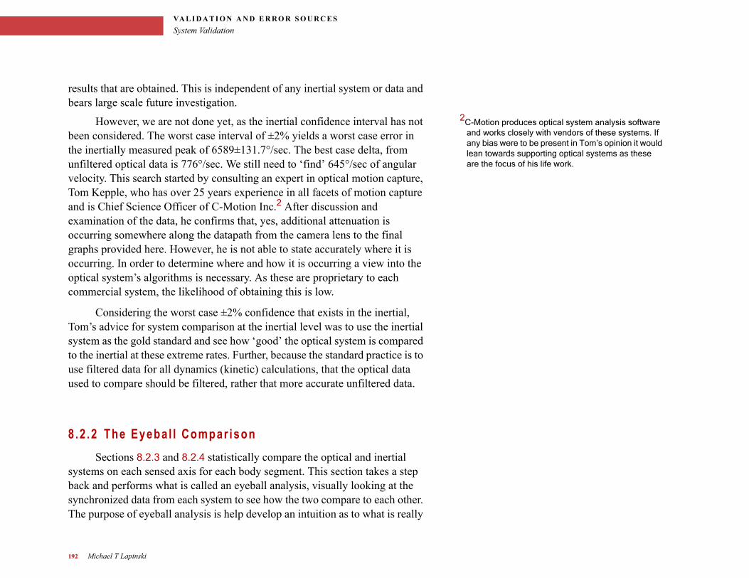
VA L I D A T I O N A N D E R R O R S O U R C E S
System Validation
results that are obtained. This is independent of any inertial system or data and bears large scale future investigation.
2C-Motion produces optical system analysis software and works closely with vendors of these systems. If any bias were to be present in Tom’s opinion it would lean towards supporting optical systems as these are the focus of his life work.
However, we are not done yet, as the inertial confidence interval has not been considered. The worst case interval of ±2% yields a worst case error in the inertially measured peak of 6589±131.7°/sec. The best case delta, from unfiltered optical data is 776°/sec. We still need to ‘find’ 645°/sec of angular velocity. This search started by consulting an expert in optical motion capture, Tom Kepple, who has over 25 years experience in all facets of motion capture and is Chief Science Officer of C-Motion Inc.2 After discussion and examination of the data, he confirms that, yes, additional attenuation is occurring somewhere along the datapath from the camera lens to the final graphs provided here. However, he is not able to state accurately where it is occurring. In order to determine where and how it is occurring a view into the optical system’s algorithms is necessary. As these are proprietary to each commercial system, the likelihood of obtaining this is low.
Considering the worst case ±2% confidence that exists in the inertial, Tom’s advice for system comparison at the inertial level was to use the inertial system as the gold standard and see how ‘good’ the optical system is compared to the inertial at these extreme rates. Further, because the standard practice is to use filtered data for all dynamics (kinetic) calculations, that the optical data used to compare should be filtered, rather that more accurate unfiltered data.
8 .2 .2 The Eyebal l Compar ison
Sections 8.2.3 and 8.2.4 statistically compare the optical and inertial systems on each sensed axis for each body segment. This section takes a step back and performs what is called an eyeball analysis, visually looking at the synchronized data from each system to see how the two compare to each other. The purpose of eyeball analysis is help develop an intuition as to what is really
192 Michael T Lapinski
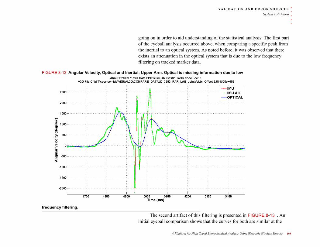
. . .
. .VA L I D A T I O N A N D E R R O R S O U R C E S
System Validation
going on in order to aid understanding of the statistical analysis. The first part of the eyeball analysis occurred above, when comparing a specific peak from the inertial to an optical system. As noted before, it was observed that there exists an attenuation in the optical system that is due to the low frequency filtering on tracked marker data.
FIGURE 8-13 Angular Velocity, Optical and Inertial; Upper Arm. Optical is missing information due to low
frequency filtering.
The second artifact of this filtering is presented in FIGURE 8-13 . An initial eyeball comparison shows that the curves for both are similar at the
A Platform for High-Speed Biomechanical Analysis Using Wearable Wireless Sensors 193
VA L I D A T I O N A N D E R R O R S O U R C E S
System Validation
beginning and end of the motion. Further comparison yields the conclusion that there is more information (more happening) in the inertial system curve while the optical curve is subdued.
The high frequency changes in the inertial curve may very well be present in raw optical data observed, however the 13Hz filter being applied is probably responsible for destroying this information. This portion of the data is most important to those studying high-speed motion, as it is where angular velocities and accelerations are high, but is missing from the optical curve. In general, this curve does not pass the eyeball comparison very well since the data we care about the most is not present and the magnitudes of highest peaks and lows are missing. This is significant because it is theorized that most stress and repetitive microtrauma occurs during peak angular velocities and accelerations. If these are undermeasured, the true severity of the trauma is also undermeasured. Again, some of these oscillations may be due to soft tissue artifacts; any exploitation of its detailed structure will need to take these into account.
194 Michael T Lapinski
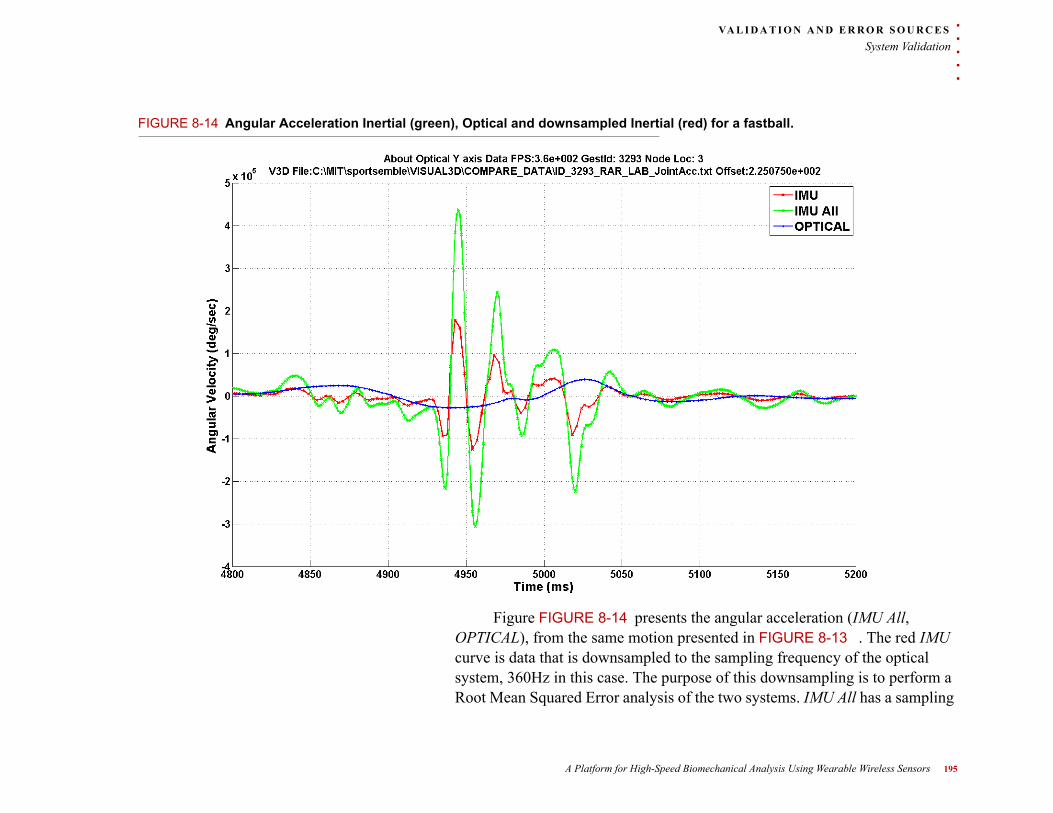
. . .
. .VA L I D A T I O N A N D E R R O R S O U R C E S
System Validation
FIGURE 8-14 Angular Acceleration Inertial (green), Optical and downsampled Inertial (red) for a fastball.
Figure FIGURE 8-14 presents the angular acceleration (IMU All, OPTICAL), from the same motion presented in FIGURE 8-13 . The red IMU curve is data that is downsampled to the sampling frequency of the optical system, 360Hz in this case. The purpose of this downsampling is to perform a Root Mean Squared Error analysis of the two systems. IMU All has a sampling
A Platform for High-Speed Biomechanical Analysis Using Wearable Wireless Sensors 195
VA L I D A T I O N A N D E R R O R S O U R C E S
System Validation
frequency of 1000Hz. Unfiltered optical angular acceleration data is not considered as it is almost all noise.
Applying the same eyeballs to these curves two things are quickly obvious. The first, that the angular acceleration calculated by the optical system is dwarfed by the IMU All angular acceleration. The explanation for this is simple, if you start with a smooth (heavily filtered) curve and differentiate the resulting curve will also be smooth. Data was destroyed in the filtering and will be lost for any future processing. The unfiltered, high frequency changes in the IMU All curve are a much better indicator of the true angular acceleration because they are based on a tight accuracy confidence interval (±2%) and directly measured angular velocity data.
The second observation that can be made is that of the effects of sampling rate on angular acceleration. The red IMU curve is downsampled to the 360Hz sampling rate of the optical system. While the red curve more closely matches the green in terms of structure, its range is closer to that of the blue optical curve. This indicates that not only does the initial filtering of the optical data effect angular acceleration results, but that sampling frequency also plays a role. It also indicates that the optical systems need to improve or that other avenues for obtaining angular velocity data to complement the optical system need to be explored.
8 .2 .3 Angular Ve loc i ty Compar ison
The root mean squared error (RMSE) and delta between maximum/minimum peaks for each gesture are the two metrics used to compare the optical system to the inertial. The RMSE is an indicator of how good the fit is between the studied gestures. The delta between the maxima/minima is an indicator of how much attenuation is occurring. Further, most biomechanical analysis focuses on peak inertial values; as they are
196 Michael T Lapinski
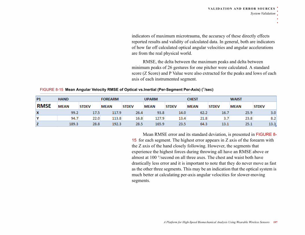
. . .
. .VA L I D A T I O N A N D E R R O R S O U R C E S
System Validation
indicators of maximum microtrauma, the accuracy of these directly effects reported results and validity of calculated data. In general, both are indicators of how far off calculated optical angular velocities and angular accelerations are from the real physical world.
RMSE, the delta between the maximum peaks and delta between minimum peaks of 26 gestures for one pitcher were calculated. A standard score (Z Score) and P Value were also extracted for the peaks and lows of each axis of each instrumented segment.
FIGURE 8-15 Mean Angular Velocity RMSE of Optical vs.Inertial (Per-Segment Per-Axis) (°/sec)
Mean RMSE error and its standard deviation, is presented in FIGURE 8-15 for each segment. The highest error appears in Z axis of the forearm with the Z axis of the hand closely following. However, the segments that experience the highest forces during throwing all have an RMSE above or almost at 100 °/second on all three axes. The chest and waist both have drastically less error and it is important to note that they do never move as fast as the other three segments. This may be an indication that the optical system is much better at calculating per-axis angular velocities for slower-moving segments.
A Platform for High-Speed Biomechanical Analysis Using Wearable Wireless Sensors 197
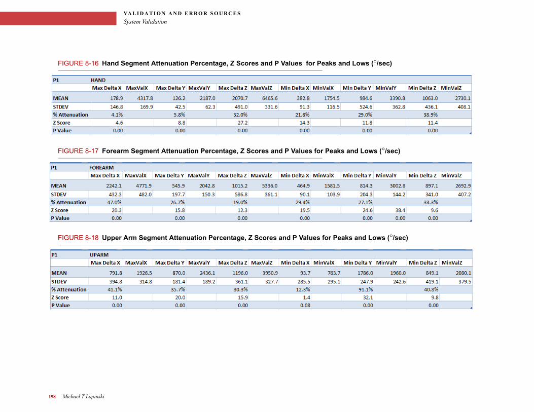
VA L I D A T I O N A N D E R R O R S O U R C E S
System Validation
FIGURE 8-16 Hand Segment Attenuation Percentage, Z Scores and P Values for Peaks and Lows (°/sec)
FIGURE 8-17 Forearm Segment Attenuation Percentage, Z Scores and P Values for Peaks and Lows (°/sec)
FIGURE 8-18 Upper Arm Segment Attenuation Percentage, Z Scores and P Values for Peaks and Lows (°/sec)
198 Michael T Lapinski
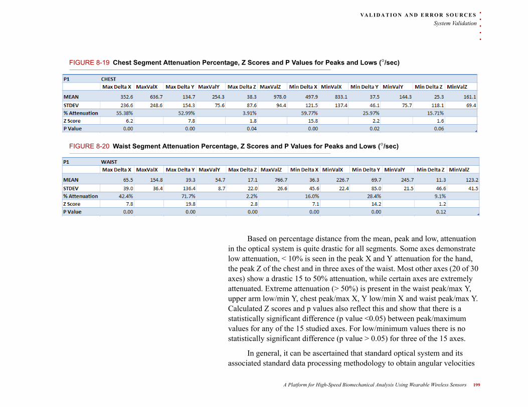
. . .
. .VA L I D A T I O N A N D E R R O R S O U R C E S
System Validation
FIGURE 8-19 Chest Segment Attenuation Percentage, Z Scores and P Values for Peaks and Lows (°/sec)
FIGURE 8-20 Waist Segment Attenuation Percentage, Z Scores and P Values for Peaks and Lows (°/sec)
Based on percentage distance from the mean, peak and low, attenuation in the optical system is quite drastic for all segments. Some axes demonstrate low attenuation, < 10% is seen in the peak X and Y attenuation for the hand, the peak Z of the chest and in three axes of the waist. Most other axes (20 of 30 axes) show a drastic 15 to 50% attenuation, while certain axes are extremely attenuated. Extreme attenuation (> 50%) is present in the waist peak/max Y, upper arm low/min Y, chest peak/max X, Y low/min X and waist peak/max Y. Calculated Z scores and p values also reflect this and show that there is a statistically significant difference (p value <0.05) between peak/maximum values for any of the 15 studied axes. For low/minimum values there is no statistically significant difference (p value > 0.05) for three of the 15 axes.
In general, it can be ascertained that standard optical system and its associated standard data processing methodology to obtain angular velocities
A Platform for High-Speed Biomechanical Analysis Using Wearable Wireless Sensors 199
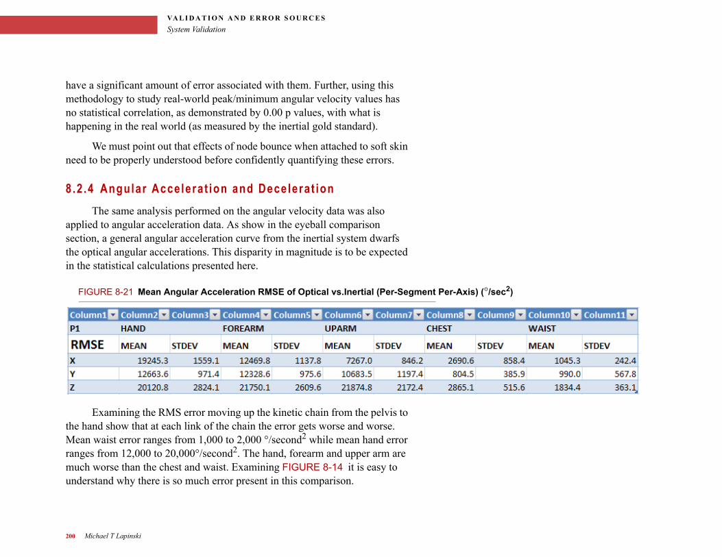
VA L I D A T I O N A N D E R R O R S O U R C E S
System Validation
have a significant amount of error associated with them. Further, using this methodology to study real-world peak/minimum angular velocity values has no statistical correlation, as demonstrated by 0.00 p values, with what is happening in the real world (as measured by the inertial gold standard).
We must point out that effects of node bounce when attached to soft skin need to be properly understood before confidently quantifying these errors.
8 .2 .4 Angular Acce lera t ion and Dece lera t ion
The same analysis performed on the angular velocity data was also applied to angular acceleration data. As show in the eyeball comparison section, a general angular acceleration curve from the inertial system dwarfs the optical angular accelerations. This disparity in magnitude is to be expected in the statistical calculations presented here.
FIGURE 8-21 Mean Angular Acceleration RMSE of Optical vs.Inertial (Per-Segment Per-Axis) (°/sec2)
Examining the RMS error moving up the kinetic chain from the pelvis to the hand show that at each link of the chain the error gets worse and worse. Mean waist error ranges from 1,000 to 2,000 °/second2 while mean hand error ranges from 12,000 to 20,000°/second2. The hand, forearm and upper arm are much worse than the chest and waist. Examining FIGURE 8-14 it is easy to understand why there is so much error present in this comparison.
200 Michael T Lapinski
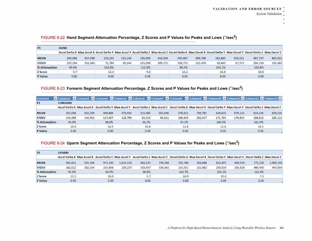
. . .
. .VA L I D A T I O N A N D E R R O R S O U R C E S
System Validation
FIGURE 8-22 Hand Segment Attenuation Percentage, Z Scores and P Values for Peaks and Lows (°/sec2)
FIGURE 8-23 Forearm Segment Attenuation Percentage, Z Scores and P Values for Peaks and Lows (°/sec2)
FIGURE 8-24 Uparm Segment Attenuation Percentage, Z Scores and P Values for Peaks and Lows (°/sec2)
A Platform for High-Speed Biomechanical Analysis Using Wearable Wireless Sensors 201
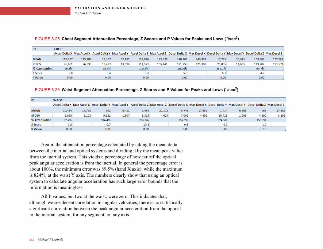
VA L I D A T I O N A N D E R R O R S O U R C E S
System Validation
FIGURE 8-25 Chest Segment Attenuation Percentage, Z Scores and P Values for Peaks and Lows (°/sec2)
FIGURE 8-26 Waist Segment Attenuation Percentage, Z Scores and P Values for Peaks and Lows (°/sec2)
Again, the attenuation percentage calculated by taking the mean delta between the inertial and optical systems and dividing it by the mean peak value from the inertial system. This yields a percentage of how far off the optical peak angular acceleration is from the inertial. In general the percentage error is about 100%, the minimum error was 89.5% (hand X axis), while the maximum is 824%, at the waist Y axis. The numbers clearly show that using an optical system to calculate angular acceleration has such large error bounds that the information is meaningless.
All P values, but two at the waist, were zero. This indicates that, although we see decent correlation in angular velocities, there is no statistically significant correlation between the peak angular acceleration from the optical to the inertial system, for any segment, on any axis.
202 Michael T Lapinski
. . .
. .A N A L Y T I C S A N D B I O M E C H A N I C A L M E T R I C S
ANALYTICS AND
BIOMECHANICAL
. . . .
. . . . . . . . . . . . . . . . . . . . . . . . . . . . . . . . . . . . . .METRICS
-
A system is only as good as the tools that are provided to analyze, manipulate and view the data that it provides. The analytics section presents a set of algorithms, tools and user interfaces for doing just this. For each tool, interface or algorithm results are also presented.
A Platform for High-Speed Biomechanical Analysis Using Wearable Wireless Sensors 203
A N A L Y T I C S A N D B I O M E C H A N I C A L M E T R I C S
Data Processing Fundamentals
. . . . . . . . . . . . . . . . . . . . . . . . . . . . . . . . . . . . . . . . . . . . . . . . . . . . . . . . . . .9 . 1 D A T A P R O C E S S I N G F U N D A M E N T A L S
Guidelines for processing data were laid out in Section1.3.3. These include three abilities (Viewability, Aggregatability and Repeatability) and one ality (Neutrailty).
Neutrality and repeatability are fulfilled by a set of data access application programming interfaces (APIs) that were developed for C/C++, Matlab and Visual Basic. These APIs abstract away the complex data model (presented in Section 6.3) and its underlying PostgresSQL relational database in an object oriented manner and allow uniform access to the data on the level of Players, Sessions and Gestures. The analyst developing algorithms only has to think at this level to access and manipulate data.
Graphical user interfaces, such as the Data Processing and Import Application, leverage the Visual Basic API and allow for viewability. Further viewability is enabled by the system’s integration with Visual3D, which uses the C++ API to import data, then further process it and display it to the user.
The Matlab API is heavily used by numerically-intensive analysis algorithms, such as data fusion and synchronization, that perform aggregation of data and then use the API to reinsert results into the database
These four concepts will be referred to throughout this section as each interface, algorithm and tool is described.
204 Michael T Lapinski
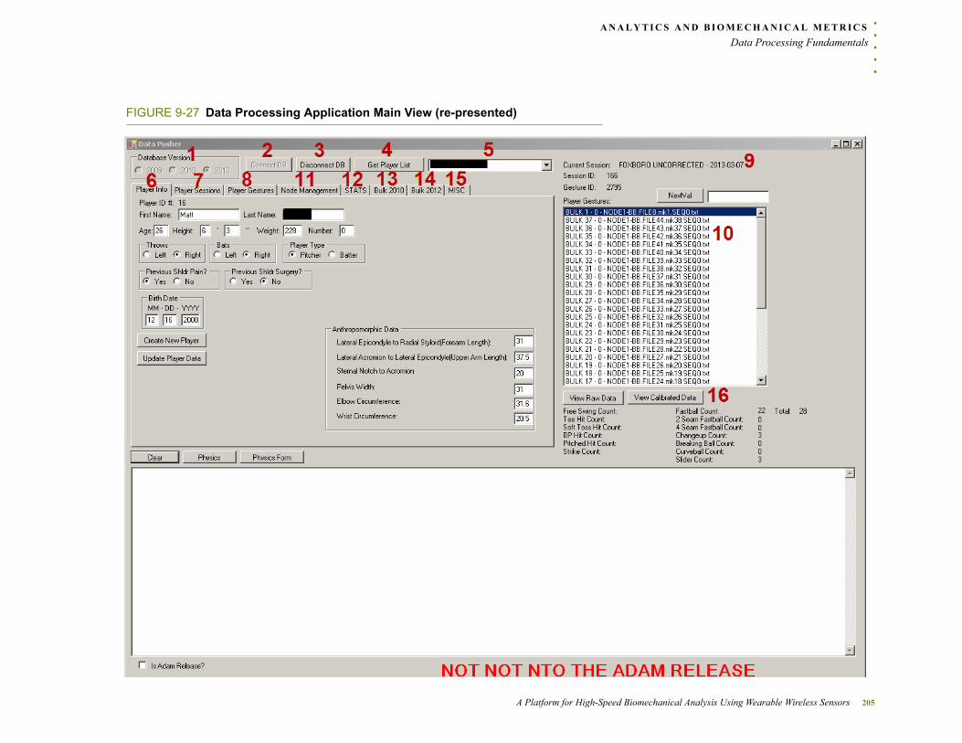
. . .
. .A N A L Y T I C S A N D B I O M E C H A N I C A L M E T R I C S
Data Processing Fundamentals
FIGURE 9-27 Data Processing Application Main View (re-presented)
A Platform for High-Speed Biomechanical Analysis Using Wearable Wireless Sensors 205
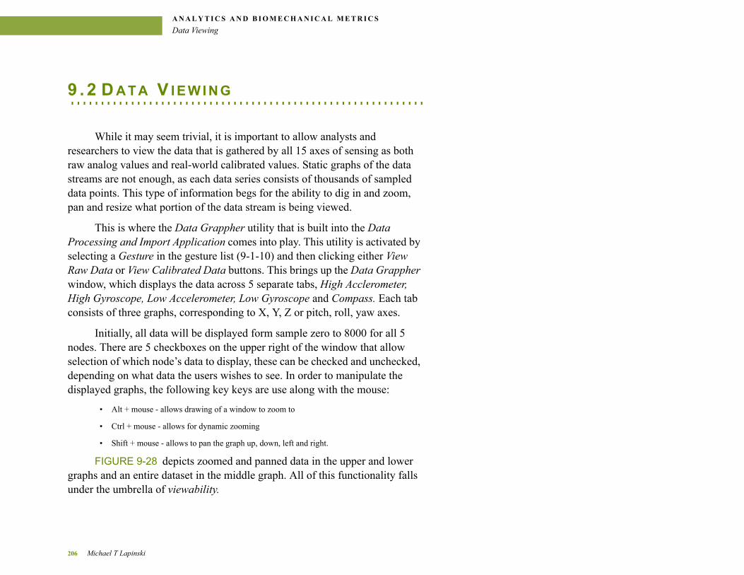
A N A L Y T I C S A N D B I O M E C H A N I C A L M E T R I C S
Data Viewing
. . . . . . . . . . . . . . . . . . . . . . . . . . . . . . . . . . . . . . . . . . . . . . . . . . . . . . . . . . .9 . 2 D A T A V I E W I N G
While it may seem trivial, it is important to allow analysts and researchers to view the data that is gathered by all 15 axes of sensing as both raw analog values and real-world calibrated values. Static graphs of the data streams are not enough, as each data series consists of thousands of sampled data points. This type of information begs for the ability to dig in and zoom, pan and resize what portion of the data stream is being viewed.
This is where the Data Grappher utility that is built into the Data Processing and Import Application comes into play. This utility is activated by selecting a Gesture in the gesture list (9-1-10) and then clicking either View Raw Data or View Calibrated Data buttons. This brings up the Data Grappher window, which displays the data across 5 separate tabs, High Acclerometer, High Gyroscope, Low Accelerometer, Low Gyroscope and Compass. Each tab consists of three graphs, corresponding to X, Y, Z or pitch, roll, yaw axes.
Initially, all data will be displayed form sample zero to 8000 for all 5 nodes. There are 5 checkboxes on the upper right of the window that allow selection of which node’s data to display, these can be checked and unchecked, depending on what data the users wishes to see. In order to manipulate the displayed graphs, the following key keys are use along with the mouse:
• Alt + mouse - allows drawing of a window to zoom to
• Ctrl + mouse - allows for dynamic zooming
• Shift + mouse - allows to pan the graph up, down, left and right.
FIGURE 9-28 depicts zoomed and panned data in the upper and lower graphs and an entire dataset in the middle graph. All of this functionality falls under the umbrella of viewability.
206 Michael T Lapinski
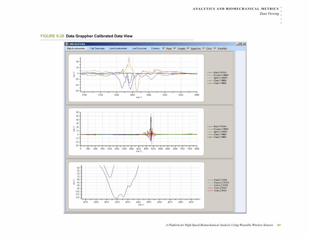
. . .
. .A N A L Y T I C S A N D B I O M E C H A N I C A L M E T R I C S
Data Viewing
FIGURE 9-28 Data Grappher Calibrated Data View
A Platform for High-Speed Biomechanical Analysis Using Wearable Wireless Sensors 207
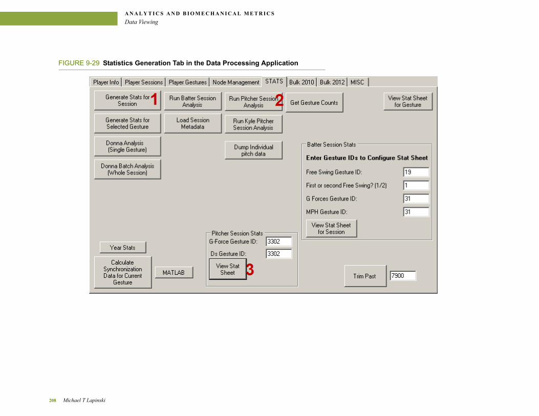
A N A L Y T I C S A N D B I O M E C H A N I C A L M E T R I C S
Data Viewing
FIGURE 9-29 Statistics Generation Tab in the Data Processing Application
208 Michael T Lapinski
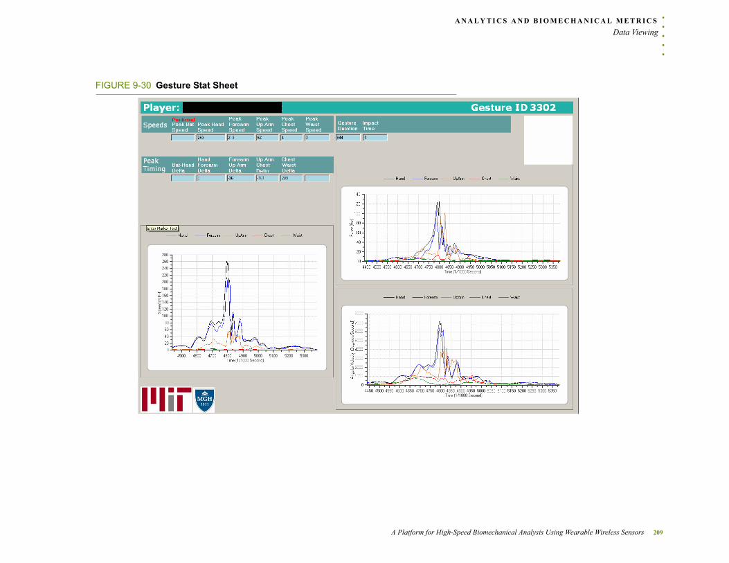
. . .
. .A N A L Y T I C S A N D B I O M E C H A N I C A L M E T R I C S
Data Viewing
FIGURE 9-30 Gesture Stat Sheet
A Platform for High-Speed Biomechanical Analysis Using Wearable Wireless Sensors 209
A N A L Y T I C S A N D B I O M E C H A N I C A L M E T R I C S
Segment Gesture Statistics
. . . . . . . . . . . . . . . . . . . . . . . . . . . . . . . . . . . . . . . . . . . . . . . . . . . . . . . . . . .9 . 3 S E G M E N T G E S T U R E S T A T I S T I C S
Gesture analysis starts with a general analysis of each gesture that includes determining its length and then (on a per-segment basis) calculating statistics on aggregated (vector magnitude over 3 axes) data for each type of inertial sensor. This data is inserted in the database and used for future processing at the session level.
Sections 9.3.1 and 9.3.2 document what are termed general stats for a session. Their behavior is executed by clicking the Generate Stats for Session (9-3-1) button under the STATS tab in the Data Processing Application (9-1-12).
The data for any gesture is presented to clinicians, coaches and players via the Gesture Stat Sheet (FIGURE 9-30 ). This sheet contains the extrapolated segment speeds in miles per hour and the timing deltas between the peaks of each segment’s speed. Three graphs are also presented: vector magnitude acceleration, angular velocity and extrapolated speeds for each segment. Lastly, the calculated gesture duration and impact time (for swings) is also displayed.
9 .3 .1 Gesture Durat ion Determinat ion
As the inertial system is at millisecond granularity, it is an excellent platform for examining the amount of time that a single pitch or swing takes to execute. Further, having an algorithmic process for trimming any unnecessary data from a gesture allows for analysis to focus on only the relevant motion contained in the inertial data streams.
This algorithm finds the peak for the vector magnitude of all the axes (gyroscope or accelerometer) and iterates backwards and forwards until the
210 Michael T Lapinski
. . .
. .A N A L Y T I C S A N D B I O M E C H A N I C A L M E T R I C S
Segment Gesture Statistics
inertial value falls below a given threshold. For gyroscopes, 300 degrees/second and accelerometers 3.2G’s. Iterating backwards from the peak yields a sensor specific start time for each gesture in terms of gyroscope and accelerometer. The minimum of these two values is taken and is used as the start time of the gesture. The same process occurs iterating forward, however the maximum value of the two is taken as the end time for the gesture.
This process is applied for all body segments and rolled up into a gesture-level start and end time by taking the minimum of all segment start times and maximum of each segment end time, respectively. This information is stored in the database as part of the gesture metadata that is presented in Section 6.3.3, Gesture Data Model.
9 .3 .2 Ind iv idua l Segment Analys is
Two vector magnitudes, one of the three axes of accelerometers and one of the gyroscope’s three axes, are used to calculate and present most metrics. The reasoning behind this is twofold. First, because it represents the integrated acceleration and angular velocity, giving an general idea of how much motion is occurring at each segment. Secondly, it is much easier to have two numbers per segment when looking at general statistics instead of six per segment. For a five node upper body network, there are 10 numbers that represent the motion, rather than 30.
For each sample of each segment of each gesture the vector magnitude is calculated for the gyroscope axes and the accelerometer axes. The formula for an individual datapoint’s vector magnitude is:
magnitude X2
Y2
Z+2
+=
where X, Y and Z are accelerometer axes of gyroscope pitch roll and yaw values
A Platform for High-Speed Biomechanical Analysis Using Wearable Wireless Sensors 211
A N A L Y T I C S A N D B I O M E C H A N I C A L M E T R I C S
Segment Gesture Statistics
Once the magnitude has been calculated over all samples, for both types of sensor, the peak value is found along with the time that the peak occurred. This data is inserted into the database as part of the Gesture Data Model, Section 6.3.3.
9 .3 .3 In ter -Segment T iming
Inter-segment peak timing is calculated on the fly from the data that is stored for each segment in the previous section. The time differences between segment peaks are considered by trainers and coaches as an indicator of how well a pitcher or batter delivers power through the kinetic chain to the bat or ball. The smaller the difference, the more efficiently the power is delivered. The deltas are calculated between each pair of segments in the kinetic chain. The segment timing application (Section 9.4.2) was developed to study this phenomena in detail.
9 .3 .4 Segment Ve loc i ty Est imat ion
Segment velocity estimation is a tool that is used to translate angular velocity into lay terms. The approach is named an estimation because it makes one broad assumption about the mechanical structure of the arm when it is swinging or throwing. This assumption is that the arm is fully extended at the peak of the gesture, and allows for a simplified calculation of segment speed based on each inertial node’s location in the segment. Node location is measured and stored in the database as part of session annotation, thus these number are readily available. The derived formula for converting the
212 Michael T Lapinski
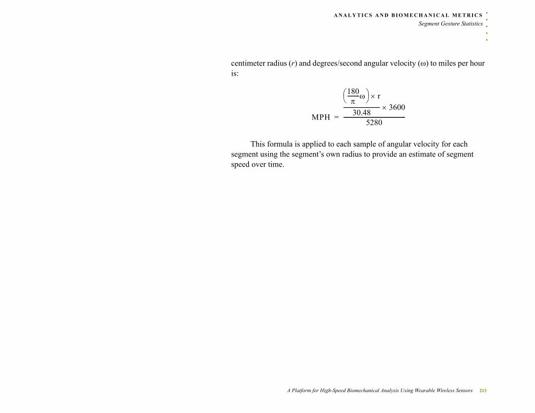
. . .
. .A N A L Y T I C S A N D B I O M E C H A N I C A L M E T R I C S
Segment Gesture Statistics
centimeter radius (r) and degrees/second angular velocity (ω) to miles per hour is:
MPH
180
--------- r
30.48--------------------------- 3600
5280----------------------------------------------=
This formula is applied to each sample of angular velocity for each segment using the segment’s own radius to provide an estimate of segment speed over time.
A Platform for High-Speed Biomechanical Analysis Using Wearable Wireless Sensors 213
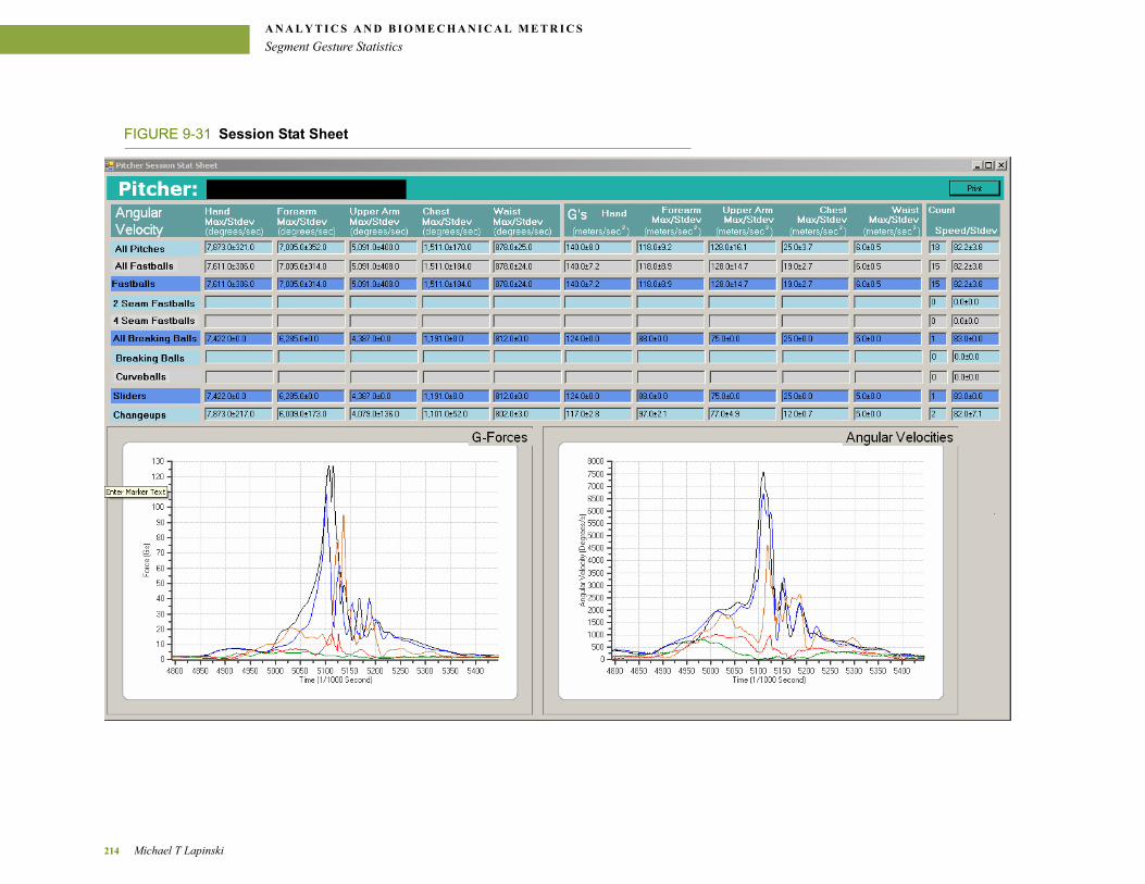
A N A L Y T I C S A N D B I O M E C H A N I C A L M E T R I C S
Segment Gesture Statistics
FIGURE 9-31 Session Stat Sheet
214 Michael T Lapinski
. . .
. .A N A L Y T I C S A N D B I O M E C H A N I C A L M E T R I C S
Session Aggregation and Statistics
9 . 4 S E S S I O N A G G R E G A T I O N A N D
. . . . . . . . . . . . . . . . . . . . . . . . . . . . . . . . . . . . . . . . . . . . . . . . . . . . . . . . . . .S T A T I S T I C S
9.4 .1 Sess ion Sta t Sheet
For each player’s session, metrics are generated to give insight into what the inertial forces and angular velocities are for different groupings of pitches and all pitches for that session. Session level data depends on what is calculated in the previous section and is a second level of post-processing. This data is presented to clinicians, coaches or players in the form of a graphical Session Stat Sheet (FIGURE 9-31 ).
The data access API allows for selection of gestures based on their type. Type is defined by the annotation and classification process that occurs at the time gesture data is inserted in the database. This feature is leveraged to first select all pitches, then the subcategory of all fastballs, then the sub-sub-category of all 2 seam fastballs, then the sub-sub-category of all 4 seam fastballs. This same behavior applies to all breaking balls and their sub-sub-categories of breaking balls and curveballs. Sliders and changeups are individual sub-categories.
Each of these selections yields a group of pitches and the metadata that was generated and stored. at the gesture level. For each selection’s gesture and each segment, the mean angular velocity and the standard deviation are calculated. The same calculations are performed for accelerations.
The analysis is executed by clicking the Run Pitcher Session Analysis button (9-3-2). Its resulting data is stored in the database as part of session metadata, Section 6.3.2. When the View Stat Sheet button (9-3-3) is clicked, the Session Stat Sheet stat sheet is displayed populated with the calculated data. The two graphs in the stat sheet are user-selectable gestures that are displayed
A Platform for High-Speed Biomechanical Analysis Using Wearable Wireless Sensors 215
A N A L Y T I C S A N D B I O M E C H A N I C A L M E T R I C S
Session Aggregation and Statistics
in vector magnitude form in units of Gs and angular velocity. Lastly, the number of pitches in each pitch category and the mean pitch speed are in the leftmost column.
The pitcher stats sheet allows for instant comparison of per-segment angular velocities and accelerations for different pitch types. This analysis takes only a couple of minutes and is a large step forward in terms of en masse data analysis. The same algorithms can be applied to hundreds of pitches and enable a big data approach to pitching analysis previously not possible.
For the particular pitcher presented in (FIGURE 9-31 ), one can quickly ascertain that, for fastballs, the acceleration the upper arm experiences are higher than those of the forearm: mean 128G upper arm vs. mean 118G forearm. For all other pitch types the mean accelerations are always less in the forearm than the upper arm.
216 Michael T Lapinski
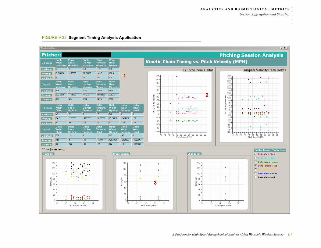
. . .
. .A N A L Y T I C S A N D B I O M E C H A N I C A L M E T R I C S
Session Aggregation and Statistics
FIGURE 9-32 Segment Timing Analysis Application
A Platform for High-Speed Biomechanical Analysis Using Wearable Wireless Sensors 217
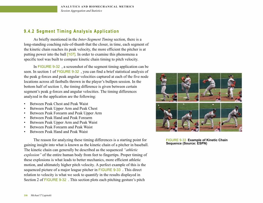
A N A L Y T I C S A N D B I O M E C H A N I C A L M E T R I C S
Session Aggregation and Statistics
9 .4 .2 Segment T iming Analys is Appl ica t ion
As briefly mentioned in the Inter-Segment Timing section, there is a long-standing coaching rule-of-thumb that the closer, in time, each segment of the kinetic chain reaches its peak velocity, the more efficient the pitcher is at putting power into the ball [107]. In order to examine this phenomena a specific tool was built to compare kinetic chain timing to pitch velocity.
In FIGURE 9-32 , a screenshot of the segment timing application can be seen. In section 1 of FIGURE 9-32 , you can find a brief statistical analysis of the peak g-forces and peak angular velocities captured at each of the five node locations across all fastballs thrown in the player’s bullpen session. In the bottom half of section 1, the timing difference is given between certain segment’s peak g-forces and angular velocities. The timing differences analyzed in the application are the following:
• Between Peak Chest and Peak Waist• Between Peak Upper Arm and Peak Chest• Between Peak Forearm and Peak Upper Arm• Between Peak Hand and Peak Forearm• Between Peak Upper Arm and Peak Waist• Between Peak Forearm and Peak Waist• Between Peak Hand and Peak Waist
FIGURE 9-33 Example of Kinetic Chain Sequence (Source: ESPN)
The reason for analyzing these timing differences is a starting point for gaining insight into what is known as the kinetic chain of a pitcher in baseball. The kinetic chain can generally be described as the sequenced “athletic explosion” of the entire human body from feet to fingertips. Proper timing of these explosions is what leads to better mechanics, more efficient athletic motion, and ultimately higher pitch velocity. A perfect example of this is the sequenced picture of a major league pitcher in FIGURE 9-33 . This direct relation to velocity is what we seek to quantify in the results displayed in Section 2 of FIGURE 9-32 . This section plots each pitching gesture’s pitch
218 Michael T Lapinski
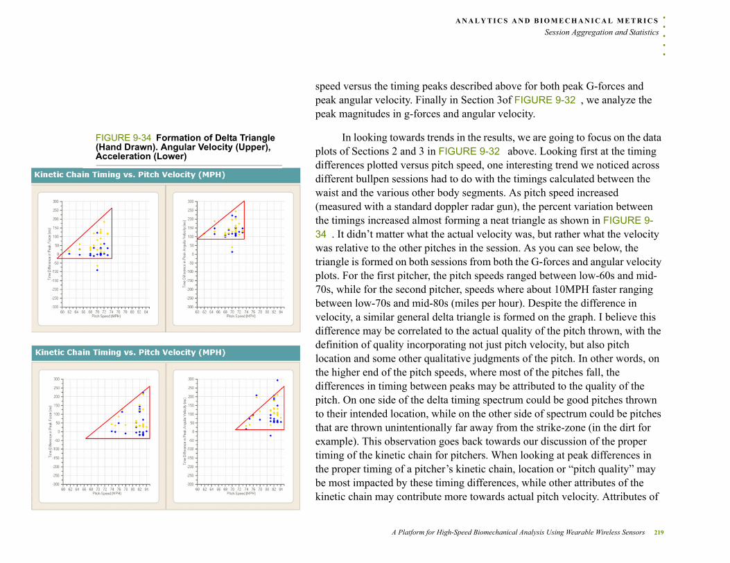
. . .
. .A N A L Y T I C S A N D B I O M E C H A N I C A L M E T R I C S
Session Aggregation and Statistics
speed versus the timing peaks described above for both peak G-forces and peak angular velocity. Finally in Section 3of FIGURE 9-32 , we analyze the peak magnitudes in g-forces and angular velocity.
FIGURE 9-34 Formation of Delta Triangle (Hand Drawn). Angular Velocity (Upper), Acceleration (Lower)
In looking towards trends in the results, we are going to focus on the data plots of Sections 2 and 3 in FIGURE 9-32 above. Looking first at the timing differences plotted versus pitch speed, one interesting trend we noticed across different bullpen sessions had to do with the timings calculated between the waist and the various other body segments. As pitch speed increased (measured with a standard doppler radar gun), the percent variation between the timings increased almost forming a neat triangle as shown in FIGURE 9-34 . It didn’t matter what the actual velocity was, but rather what the velocity was relative to the other pitches in the session. As you can see below, the triangle is formed on both sessions from both the G-forces and angular velocity plots. For the first pitcher, the pitch speeds ranged between low-60s and mid-70s, while for the second pitcher, speeds where about 10MPH faster ranging between low-70s and mid-80s (miles per hour). Despite the difference in velocity, a similar general delta triangle is formed on the graph. I believe this difference may be correlated to the actual quality of the pitch thrown, with the definition of quality incorporating not just pitch velocity, but also pitch location and some other qualitative judgments of the pitch. In other words, on the higher end of the pitch speeds, where most of the pitches fall, the differences in timing between peaks may be attributed to the quality of the pitch. On one side of the delta timing spectrum could be good pitches thrown to their intended location, while on the other side of spectrum could be pitches that are thrown unintentionally far away from the strike-zone (in the dirt for example). This observation goes back towards our discussion of the proper timing of the kinetic chain for pitchers. When looking at peak differences in the proper timing of a pitcher’s kinetic chain, location or “pitch quality” may be most impacted by these timing differences, while other attributes of the kinetic chain may contribute more towards actual pitch velocity. Attributes of
A Platform for High-Speed Biomechanical Analysis Using Wearable Wireless Sensors 219

A N A L Y T I C S A N D B I O M E C H A N I C A L M E T R I C S
Session Aggregation and Statistics
these graphs worth exploring further would be how fast the body segments reach their peak magnitudes and how long the magnitudes are sustained using
220 Michael T Lapinski
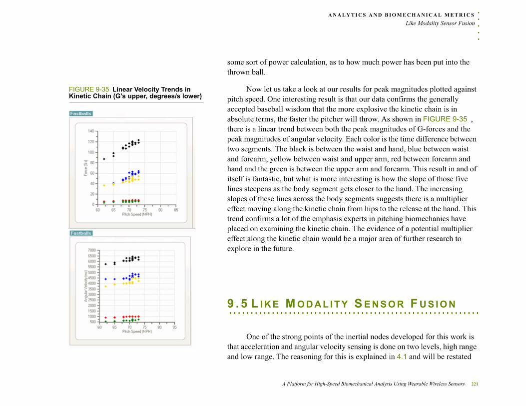
. . .
. .A N A L Y T I C S A N D B I O M E C H A N I C A L M E T R I C S
Like Modality Sensor Fusion
some sort of power calculation, as to how much power has been put into the thrown ball.
FIGURE 9-35 Linear Velocity Trends in Kinetic Chain (G’s upper, degrees/s lower)
Now let us take a look at our results for peak magnitudes plotted against pitch speed. One interesting result is that our data confirms the generally accepted baseball wisdom that the more explosive the kinetic chain is in absolute terms, the faster the pitcher will throw. As shown in FIGURE 9-35 , there is a linear trend between both the peak magnitudes of G-forces and the peak magnitudes of angular velocity. Each color is the time difference between two segments. The black is between the waist and hand, blue between waist and forearm, yellow between waist and upper arm, red between forearm and hand and the green is between the upper arm and forearm. This result in and of itself is fantastic, but what is more interesting is how the slope of those five lines steepens as the body segment gets closer to the hand. The increasing slopes of these lines across the body segments suggests there is a multiplier effect moving along the kinetic chain from hips to the release at the hand. This trend confirms a lot of the emphasis experts in pitching biomechanics have placed on examining the kinetic chain. The evidence of a potential multiplier effect along the kinetic chain would be a major area of further research to explore in the future.
. . . . . . . . . . . . . . . . . . . . . . . . . . . . . . . . . . . . . . . . . . . . . . . . . . . . . . . . . . .9 . 5 L I K E M O D A L I T Y S E N S O R F U S I O N
One of the strong points of the inertial nodes developed for this work is that acceleration and angular velocity sensing is done on two levels, high range and low range. The reasoning for this is explained in 4.1 and will be restated
A Platform for High-Speed Biomechanical Analysis Using Wearable Wireless Sensors 221
A N A L Y T I C S A N D B I O M E C H A N I C A L M E T R I C S
Like Modality Sensor Fusion
here. A high range sensor is good at sensing very fast accelerations and angular changes, but not very good at sensing slow moving accelerations and angular movement. A similar concept applies to the low range sensors, excellent at sensing slow moving parameters, incapable of sensing anything past their specified ranges. Thus, there is a need for both types of sensors to be present on inertial nodes for high-speed activity. The presence of both like sensing modalities requires that at some point data processing algorithms stop using the low range data and begin using the high range. Previous to this section, only the data based on high range sensors has been used. As the high range sensor poorly senses low range information (< 1,000 degrees/s gyroscope, < 16Gs accelerometer) there is too much variability (noise) in the high range to simply create a rule-based system of thresholds for when to use which sensor. This technique was initially attempted by the author and produced a system with so many rules and caveats that it became untractable while still producing poor fusion.
The second try at addressing the problem was with the help of the Responsive Environments Research Assistant Matt Aldrich. Matt suggested a statistical approach that calculated blending factors for each dataset to be merged and can be generically applied to any two datasets.
222 Michael T Lapinski
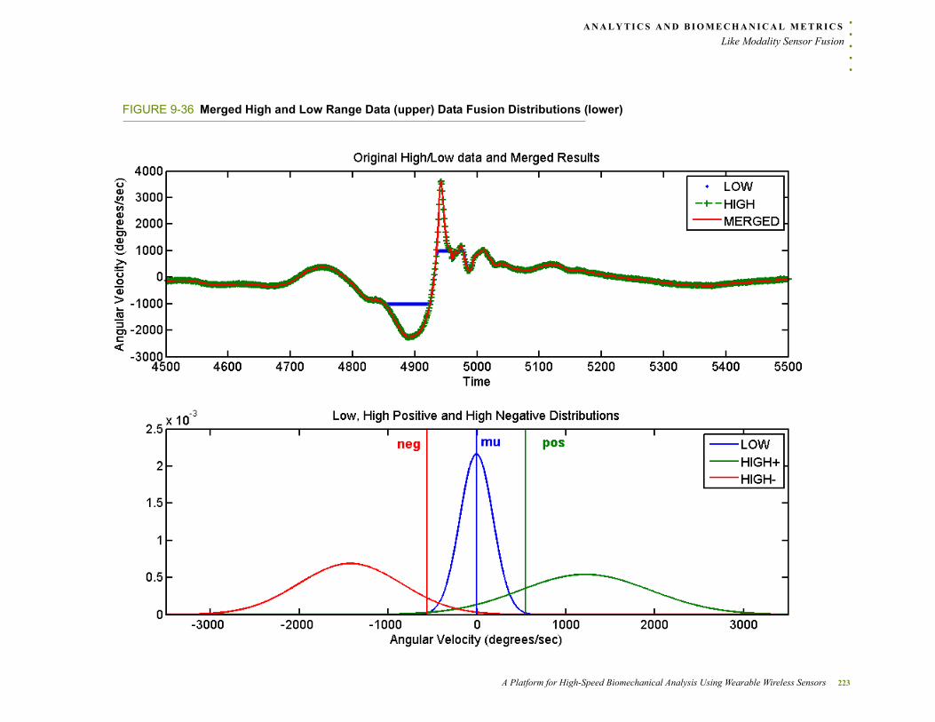
. . .
. .A N A L Y T I C S A N D B I O M E C H A N I C A L M E T R I C S
Like Modality Sensor Fusion
FIGURE 9-36 Merged High and Low Range Data (upper) Data Fusion Distributions (lower)
A Platform for High-Speed Biomechanical Analysis Using Wearable Wireless Sensors 223
A N A L Y T I C S A N D B I O M E C H A N I C A L M E T R I C S
Like Modality Sensor Fusion
The process starts with two vectors of data, high range and low range. Using the low range data, a normal distribution is generated, yielding a mu (μ) and sigma-squared (σ2) value. These two parameters are matched with a user-defined tuning parameter (final value of 3) to define two dividing thresholds for the high range data. The formula for determining the thresholds is:
threshold P 2 =
where P is the tuning parameter and ± is dependant on whether positive of negative high range calculations are being made. The thresholds, along with μ, are show in FIGURE 9-36 as vertical lines neg, mu and pos in the lower graph.
In the next step, high range data is partitioned into positive and negative. The partitioning is based on the thresholds; all data less than neg is put into one partition and above pos is placed into a second. This effectively removes any data that is ± P standard deviations from μ in the high data. Using the partitioned positive and negative data, two more normal distributions are fit.
Now there are three distributions: positive high, low and negative high, and two original sets of data: high and low.
The probability density function for each distribution is calculated using low range data with the low normal distribution and all high data for both positive and negative distributions. This effectively gives a weight for each datapoint in the low dataset and two weights for each high-range data point in the form of 3 vectors of data, distHiPos, distLo, distHiNeg. These weights are applied to their respective data sets and the results are summed. The general equation for this is:
224 Michael T Lapinski
. . .
. .A N A L Y T I C S A N D B I O M E C H A N I C A L M E T R I C S
Biomechanical Metrics
valuen hiDatan distHiNegn lowDatan distLon hiDatan distHiPosn + +=
where hiData is the high-range sensor data and lowData is the low-range sensor data.
It is important to note that, because of how the distributions are generated, the weight for a positive high value will be zero in the negative weight vector and vice versa. Moreover, the weights where the distributions intersect will create a blending effect on the data and the end effect is a smooth fusion that is dependant on the actual data itself, not predetermined thresholds. Resultant data is shown in the upper graph of FIGURE 9-36 .
. . . . . . . . . . . . . . . . . . . . . . . . . . . . . . . . . . . . . . . . . . . . . . . . . . . . . . . . . . .9 . 6 B I O M E C H A N I C A L M E T R I C S
Session and gesture level analysis and data presentation both are in the category of data viewability and aggregatabiliy. This section will explore some metrics that are relevant to traditional biomechanical analysis that are published in orthopedic literature.
A Platform for High-Speed Biomechanical Analysis Using Wearable Wireless Sensors 225
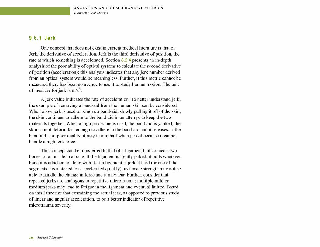
A N A L Y T I C S A N D B I O M E C H A N I C A L M E T R I C S
Biomechanical Metrics
9 .6 .1 Jerk
One concept that does not exist in current medical literature is that of Jerk, the derivative of acceleration. Jerk is the third derivative of position, the rate at which something is accelerated. Section 8.2.4 presents an in-depth analysis of the poor ability of optical systems to calculate the second derivative of position (acceleration); this analysis indicates that any jerk number derived from an optical system would be meaningless. Further, if this metric cannot be measured there has been no avenue to use it to study human motion. The unit of measure for jerk is m/s3.
A jerk value indicates the rate of acceleration. To better understand jerk, the example of removing a band-aid from the human skin can be considered. When a low jerk is used to remove a band-aid, slowly pulling it off of the skin, the skin continues to adhere to the band-aid in an attempt to keep the two materials together. When a high jerk value is used, the band-aid is yanked, the skin cannot deform fast enough to adhere to the band-aid and it releases. If the band-aid is of poor quality, it may tear in half when jerked because it cannot handle a high jerk force.
This concept can be transferred to that of a ligament that connects two bones, or a muscle to a bone. If the ligament is lightly jerked, it pulls whatever bone it is attached to along with it. If a ligament is jerked hard (or one of the segments it is atatched to is accelerated quickly), its tensile strength may not be able to handle the change in force and it may tear. Further, consider that repeated jerks are analogous to repetitive microtrauma; multiple mild or medium jerks may lead to fatigue in the ligament and eventual failure. Based on this I theorize that examining the actual jerk, as opposed to previous study of linear and angular acceleration, to be a better indicator of repetitive microtrauma severity.
226 Michael T Lapinski

. . .
. .A N A L Y T I C S A N D B I O M E C H A N I C A L M E T R I C S
Biomechanical Metrics
Which component of jerk and how it can be used in biomechanical study is an unanswered question. Here we will present the first jerk data taken for the human body and some related metrics with their analysis.
Note that STA’s may contribute to this data; future work must ascertain the magnitude of these effects.
A Platform for High-Speed Biomechanical Analysis Using Wearable Wireless Sensors 227
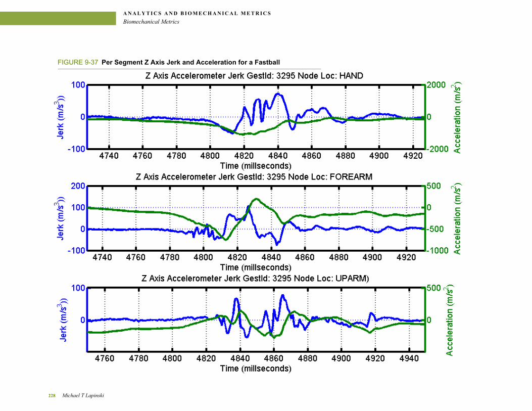
A N A L Y T I C S A N D B I O M E C H A N I C A L M E T R I C S
Biomechanical Metrics
FIGURE 9-37 Per Segment Z Axis Jerk and Acceleration for a Fastball
228 Michael T Lapinski
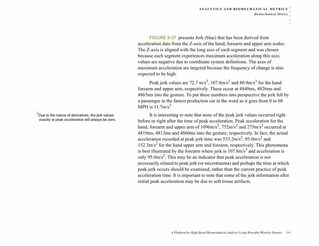
. . .
. .A N A L Y T I C S A N D B I O M E C H A N I C A L M E T R I C S
Biomechanical Metrics
FIGURE 9-37 presents Jerk (blue) that has been derived from acceleration data from the Z-axis of the hand, forearm and upper arm nodes. The Z-axis is aligned with the long axis of each segment and was chosen because each segment experiences maximum acceleration along this axis; values are negative due to coordinate system definitions. The axes of maximum acceleration are targeted because the frequency of change is also expected to be high.
Peak jerk values are 72.7 m/s3, 107.8m/s3 and 80.9m/s3 for the hand forearm and upper arm, respectively. These occur at 4840ms, 4826ms and 4865ms into the gesture. To put these numbers into perspective the jerk felt by a passenger in the fastest production car in the word as it goes from 0 to 60 MPH is 11.7m/s3
3Due to the nature of derivatives, the jerk values exactly at peak acceleration will always be zero.
It is interesting to note that none of the peak jerk values occurred right before or right after the time of peak acceleration. Peak acceleration for the hand, forearm and upper arm of 1096m/s2, 752m/s2 and 275m/s2 occurred at 4819ms, 4813ms and 4860ms into the gesture, respectively. In fact, the actual acceleration recorded at peak jerk time was 553.2m/s2, 95.0m/s2 and 152.3m/s2 for the hand upper arm and forearm, respectively. This phenomena is best illustrated by the forearm where jerk is 107.8m/s3 and acceleration is only 95.0m/s2. This may be an indicator that peak acceleration is not necessarily related to peak jerk (or microtrauma) and perhaps the time at which peak jerk occurs should be examined, rather than the current practice of peak acceleration time. It is important to note that some of the jerk information after initial peak acceleration may be due to soft tissue artifacts.
A Platform for High-Speed Biomechanical Analysis Using Wearable Wireless Sensors 229
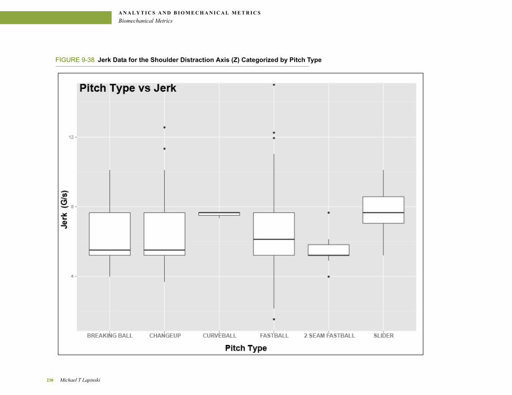
A N A L Y T I C S A N D B I O M E C H A N I C A L M E T R I C S
Biomechanical Metrics
FIGURE 9-38 Jerk Data for the Shoulder Distraction Axis (Z) Categorized by Pitch Type
230 Michael T Lapinski
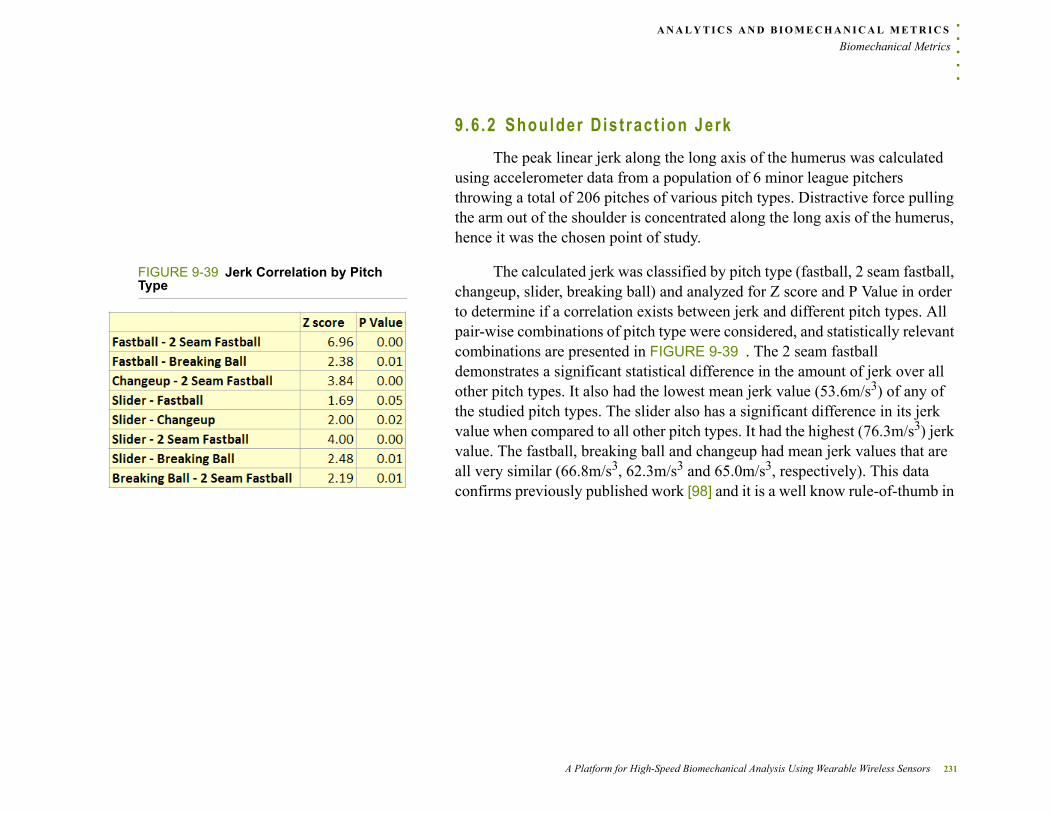
. . .
. .A N A L Y T I C S A N D B I O M E C H A N I C A L M E T R I C S
Biomechanical Metrics
9 .6 .2 Shoulder D is t ract ion Jerk
The peak linear jerk along the long axis of the humerus was calculated using accelerometer data from a population of 6 minor league pitchers throwing a total of 206 pitches of various pitch types. Distractive force pulling the arm out of the shoulder is concentrated along the long axis of the humerus, hence it was the chosen point of study.
FIGURE 9-39 Jerk Correlation by Pitch Type
The calculated jerk was classified by pitch type (fastball, 2 seam fastball, changeup, slider, breaking ball) and analyzed for Z score and P Value in order to determine if a correlation exists between jerk and different pitch types. All pair-wise combinations of pitch type were considered, and statistically relevant combinations are presented in FIGURE 9-39 . The 2 seam fastball demonstrates a significant statistical difference in the amount of jerk over all other pitch types. It also had the lowest mean jerk value (53.6m/s3) of any of the studied pitch types. The slider also has a significant difference in its jerk value when compared to all other pitch types. It had the highest (76.3m/s3) jerk value. The fastball, breaking ball and changeup had mean jerk values that are all very similar (66.8m/s3, 62.3m/s3 and 65.0m/s3, respectively). This data confirms previously published work [98] and it is a well know rule-of-thumb in
A Platform for High-Speed Biomechanical Analysis Using Wearable Wireless Sensors 231
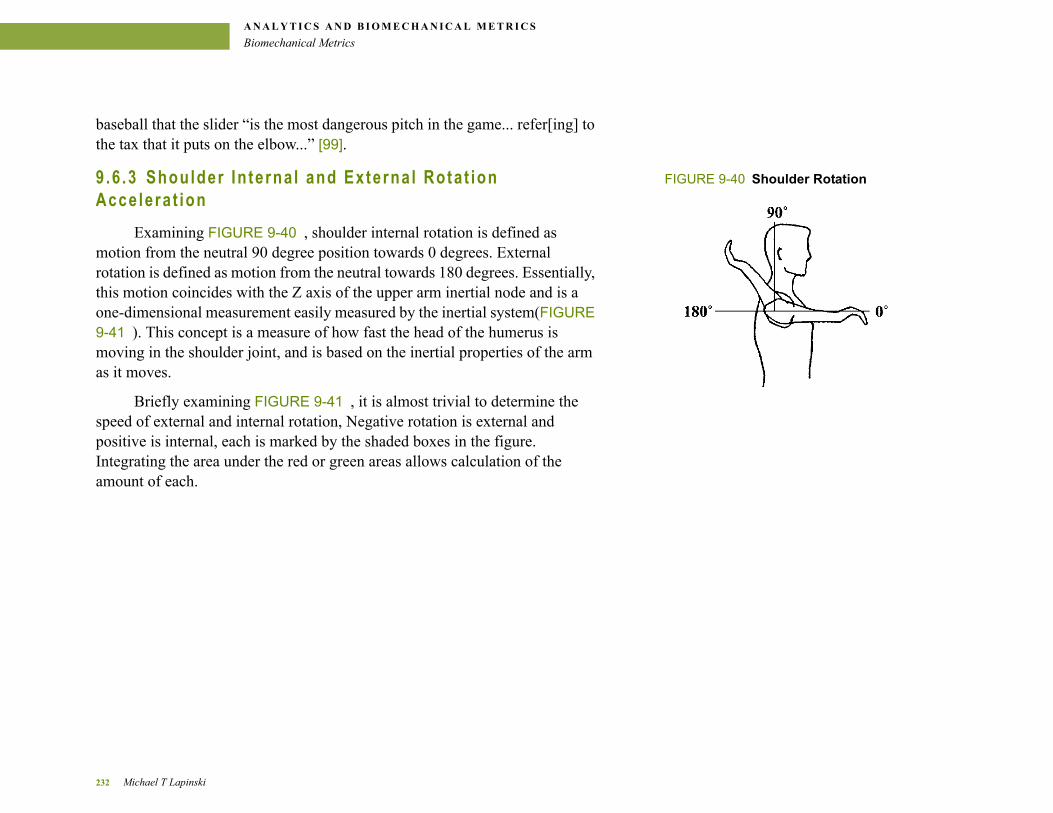
A N A L Y T I C S A N D B I O M E C H A N I C A L M E T R I C S
Biomechanical Metrics
baseball that the slider “is the most dangerous pitch in the game... refer[ing] to the tax that it puts on the elbow...” [99].
FIGURE 9-40 Shoulder Rotation9 .6 .3 Shoulder In terna l and Externa l Rota t ion Acce lera t ion
Examining FIGURE 9-40 , shoulder internal rotation is defined as motion from the neutral 90 degree position towards 0 degrees. External rotation is defined as motion from the neutral towards 180 degrees. Essentially, this motion coincides with the Z axis of the upper arm inertial node and is a one-dimensional measurement easily measured by the inertial system(FIGURE 9-41 ). This concept is a measure of how fast the head of the humerus is moving in the shoulder joint, and is based on the inertial properties of the arm as it moves.
Briefly examining FIGURE 9-41 , it is almost trivial to determine the speed of external and internal rotation, Negative rotation is external and positive is internal, each is marked by the shaded boxes in the figure. Integrating the area under the red or green areas allows calculation of the amount of each.
232 Michael T Lapinski
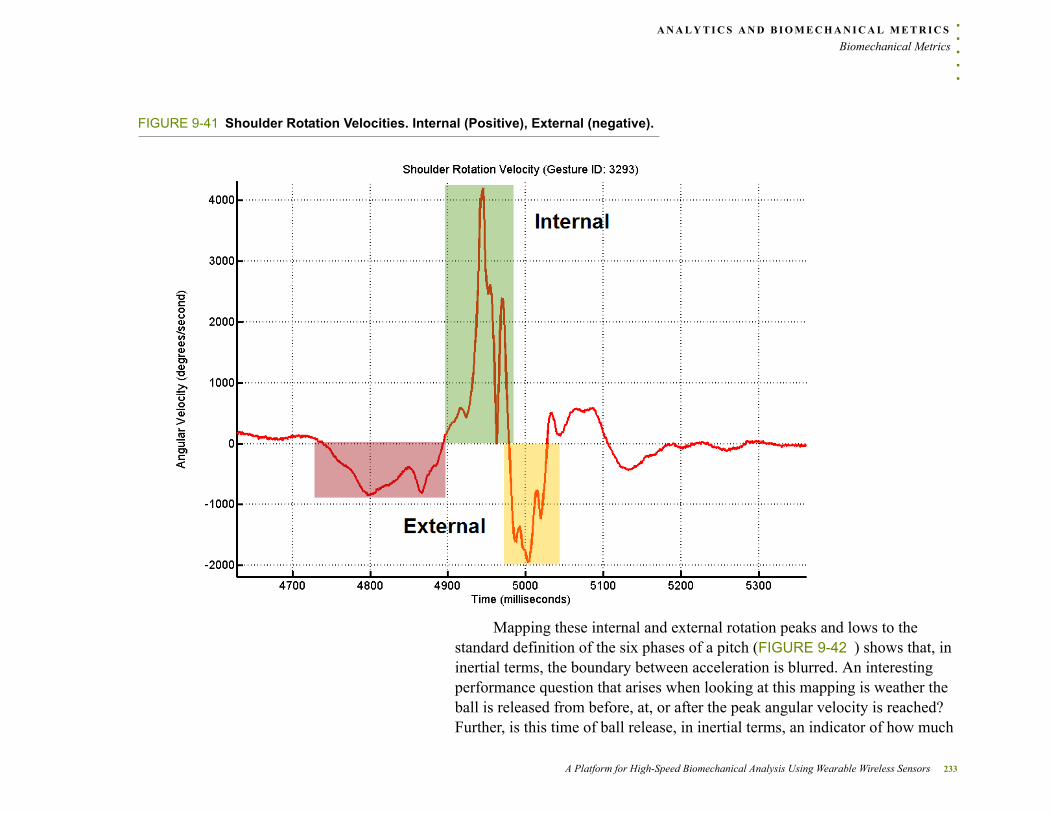
. . .
. .A N A L Y T I C S A N D B I O M E C H A N I C A L M E T R I C S
Biomechanical Metrics
FIGURE 9-41 Shoulder Rotation Velocities. Internal (Positive), External (negative).
Mapping these internal and external rotation peaks and lows to the standard definition of the six phases of a pitch (FIGURE 9-42 ) shows that, in inertial terms, the boundary between acceleration is blurred. An interesting performance question that arises when looking at this mapping is weather the ball is released from before, at, or after the peak angular velocity is reached? Further, is this time of ball release, in inertial terms, an indicator of how much
A Platform for High-Speed Biomechanical Analysis Using Wearable Wireless Sensors 233
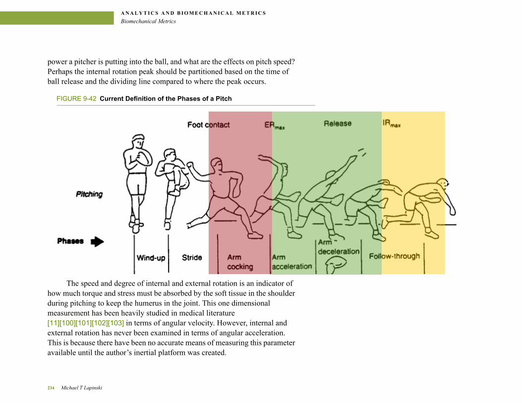
A N A L Y T I C S A N D B I O M E C H A N I C A L M E T R I C S
Biomechanical Metrics
power a pitcher is putting into the ball, and what are the effects on pitch speed? Perhaps the internal rotation peak should be partitioned based on the time of ball release and the dividing line compared to where the peak occurs.
FIGURE 9-42 Current Definition of the Phases of a Pitch
The speed and degree of internal and external rotation is an indicator of how much torque and stress must be absorbed by the soft tissue in the shoulder during pitching to keep the humerus in the joint. This one dimensional measurement has been heavily studied in medical literature [11][100][101][102][103] in terms of angular velocity. However, internal and external rotation has never been examined in terms of angular acceleration. This is because there have been no accurate means of measuring this parameter available until the author’s inertial platform was created.
234 Michael T Lapinski
. . .
. .A N A L Y T I C S A N D B I O M E C H A N I C A L M E T R I C S
Biomechanical Metrics
The internal and external rotation velocity simply parameterizes how fast the humeral head is moving inside the shoulder joint. It does not measure the acceleration and deceleration of the humeral head. The magnitude of internal and external angular acceleration, when the shoulder tissue must contain the humerus in the joint, is possibly a better indicator of the magnitude of microtrauma, rather than just velocity alone.
FIGURE 9-43 shows shoulder rotation velocity and the rate of shoulder acceleration. The peak acceleration is 370,100°/sec2 and the peak rate of deceleration -350,700°/sec2. The angular velocities at the time of these two datapoints are 3058°/sec and 1105°/sec, respectively. The delta time between these two is 20 milliseconds. This means that the humerus was accelerating at 370,100°/sec2 and within 20 milliseconds was decelerating at 350,700°/sec2. This is an acceleration delta of 720,800°/sec and indicates that during the transition from peak angular velocity during the acceleration phase to the deceleration phase the shoulder performs the maximum amount of work to stabilize the humerus and keep it in the joint.
A Platform for High-Speed Biomechanical Analysis Using Wearable Wireless Sensors 235
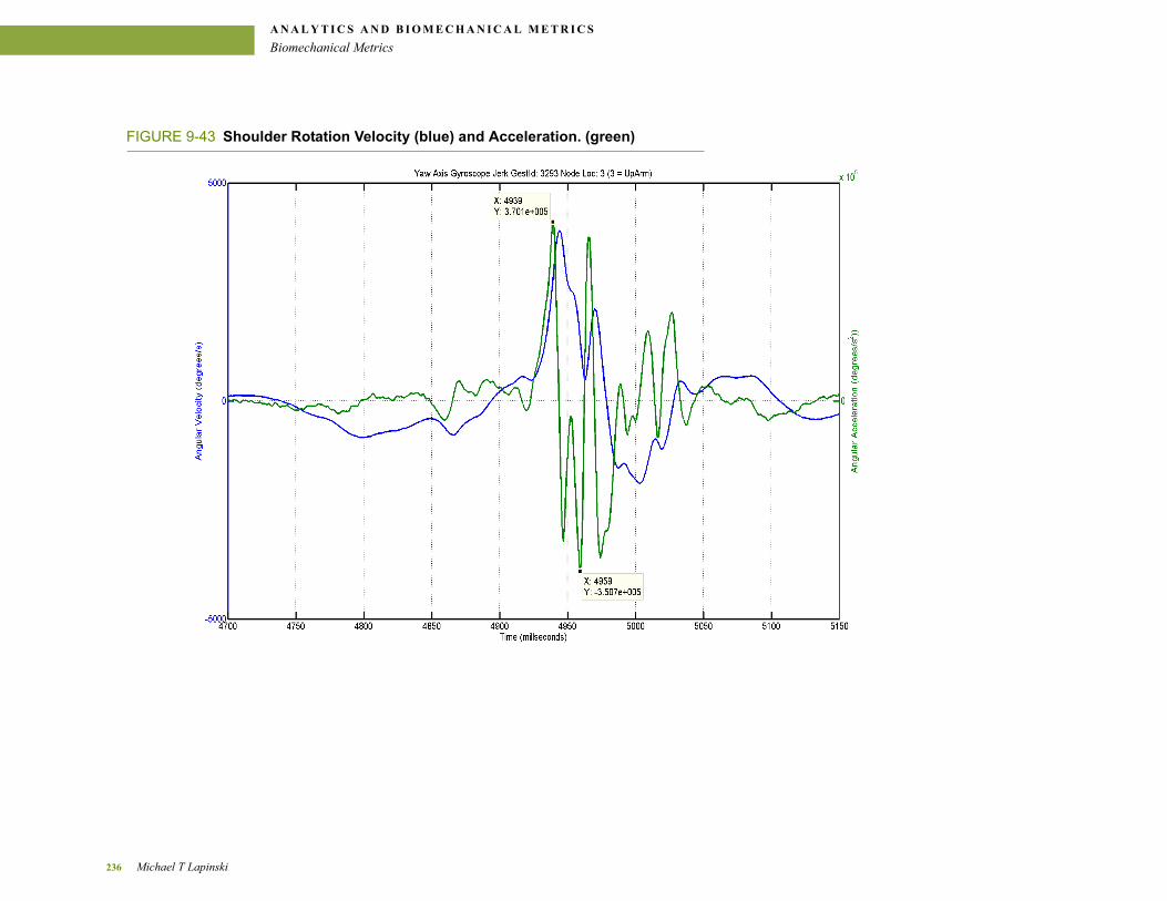
A N A L Y T I C S A N D B I O M E C H A N I C A L M E T R I C S
Biomechanical Metrics
FIGURE 9-43 Shoulder Rotation Velocity (blue) and Acceleration. (green)
236 Michael T Lapinski
. . .
. .A N A L Y T I C S A N D B I O M E C H A N I C A L M E T R I C S
Calculation of Kinetics and Dynamics
9 . 7 C A L C U L A T I O N O F K I N E T I C S A N D
. . . . . . . . . . . . . . . . . . . . . . . . . . . . . . . . . . . . . . . . . . . . . . . . . . . . . . . . . . .D Y N A M I C S
All sections of this chapter prior to this one demonstrate several medically relevant uses of the inertial network without any context for the relationships between body segments. The next level of analysis involves calculating the kinetic forces that are being experienced between the body segments at the joints. Calculation of these requires knowledge of the context between the segments, or joint angles, over time, the forces and angular velocities, centers of mass of segments and the appropriate dynamics algorithms. An architecture for doing so has been designed and is presented here.
9 .7 .1 V isua l3D In tegrat ion
C-Motion Incorporated's Visual3D is introduced in Section 3.4, It is an important part of obtaining kinetic information because the complex mechanical algorithms necessary for doing so are implemented in the software. There is no need to ‘reinvent’ the analysis and this author is not even close to being qualified to do so. However making use of the existing algorithms requires that inertial data be somehow brought into Visual3D and that data be used when specific kinetic calculations are performed.
The initial approach was to calculate orientations and joints angles for the segments using only inertial data and to import this data along with inertial data into Visual3D to create a system that is standalone from any optical tracker. The task of properly calculating joint angles for segments over time is non-trivial and a large amount of effort was put forth to realize a system such
A Platform for High-Speed Biomechanical Analysis Using Wearable Wireless Sensors 237
A N A L Y T I C S A N D B I O M E C H A N I C A L M E T R I C S
Calculation of Kinetics and Dynamics
as this. Although some commercial products on the market actually do this (i.e. XSens), the demands of our application are severe, hence the problem is much more difficult than it appears on the surface and was not solved. A detailed discussion of why is presented in the following chapter. Instead a hybrid inertial-optical system was created. This system exploits the strengths of both systems and uses the precise joint angles available from the optical tracker as the positional information when calculating kinetics. For the portions of the calculation that require accelerations, angular velocities and angular accelerations, it uses data from the inertial node sensor network. The inertial data has been shown to be more precise than optical for determining forces and torques in Chapter 8 and is the logical choice to obtaining the best results.
The first step in bringing data into Visual3D involves preprocessing it to ensure that it is synchronized with optical data. This involves reading synchronization offset information (in milliseconds) from the database and subtracting it from the inertial data. The high and low range data also need to be fused, and the algorithm for doing so is presented in Section 9.5. Angular acceleration data is calculated based on angular velocity data and filtered lightly with a 250Hz Butterworth filter to remove noise present in the derivative.
With fused and synchronized data available, a plugin to Visual3D was built that would import it from the database into the program’s memory. This data is then transformed into the same coordinate systems as the individual body segments and is available to Visual3D’s dynamics engine. This architecture is presented in FIGURE 9-44 .
238 Michael T Lapinski
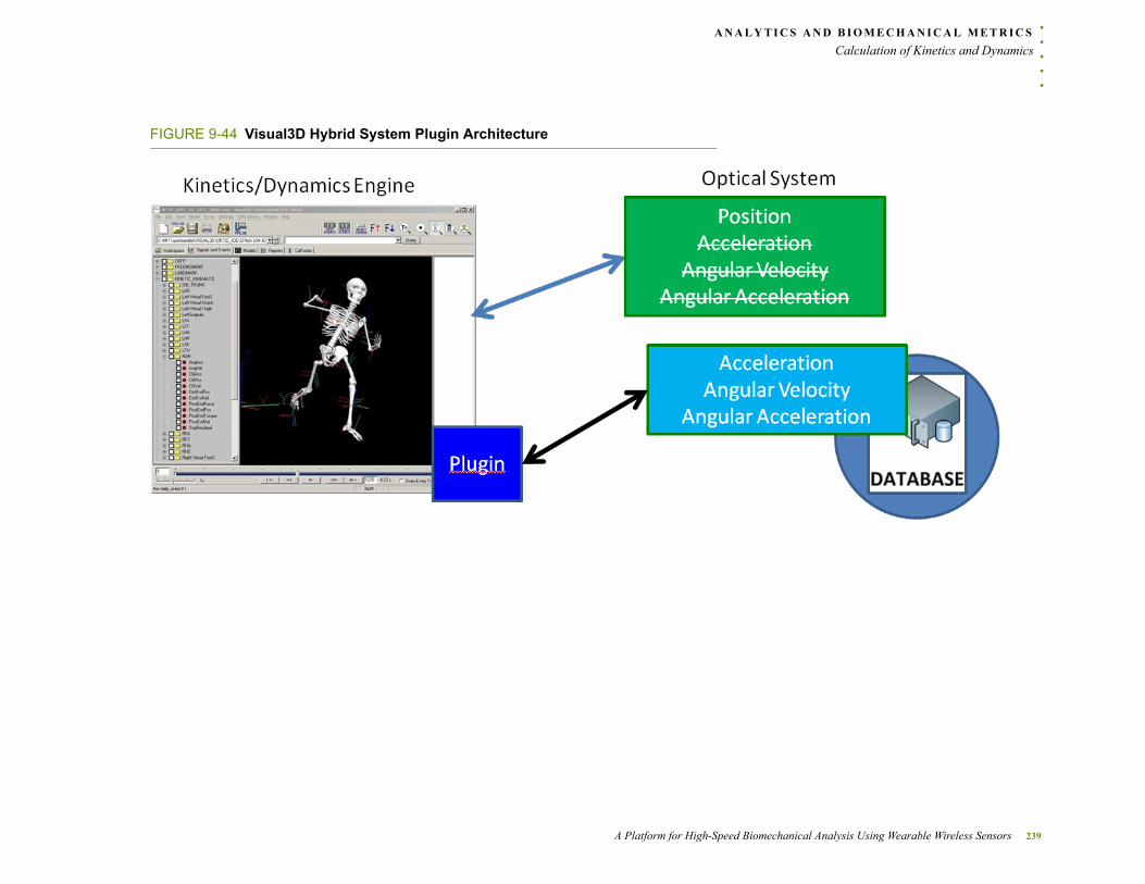
. . .
. .A N A L Y T I C S A N D B I O M E C H A N I C A L M E T R I C S
Calculation of Kinetics and Dynamics
FIGURE 9-44 Visual3D Hybrid System Plugin Architecture
A Platform for High-Speed Biomechanical Analysis Using Wearable Wireless Sensors 239
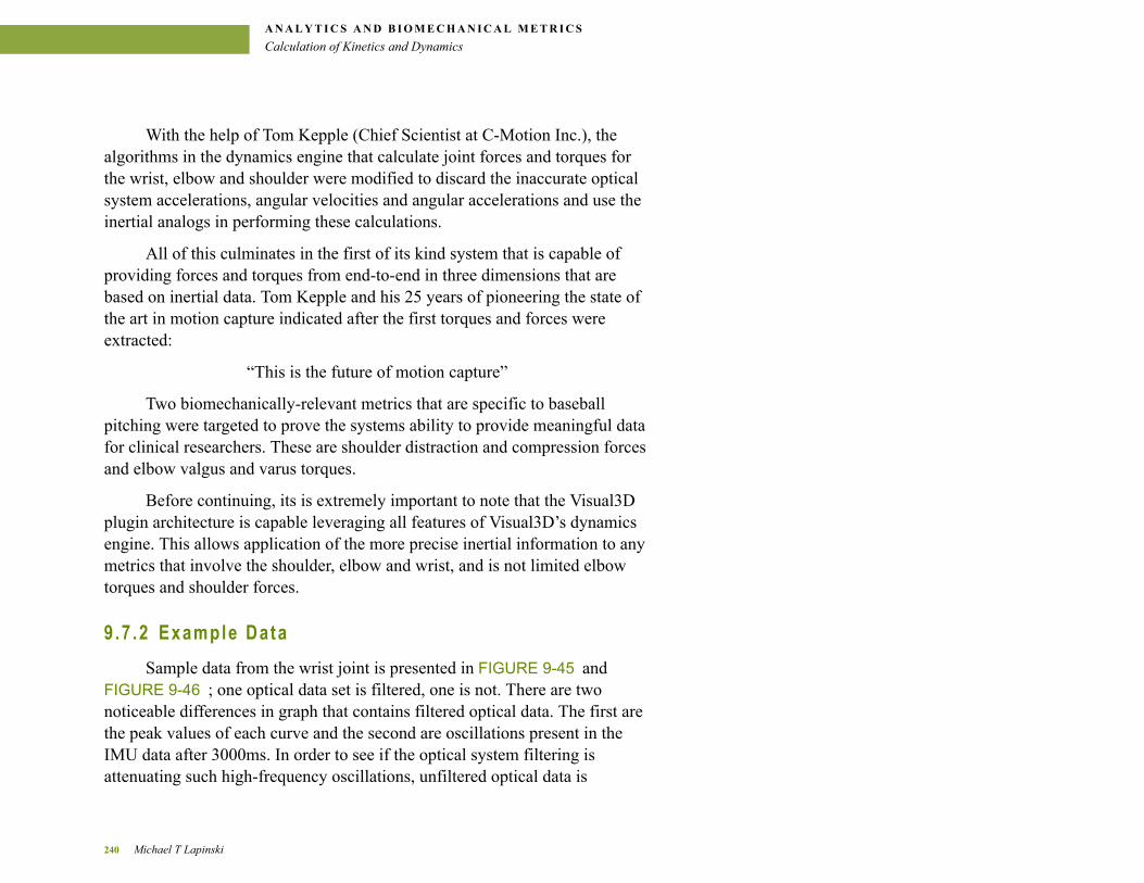
A N A L Y T I C S A N D B I O M E C H A N I C A L M E T R I C S
Calculation of Kinetics and Dynamics
With the help of Tom Kepple (Chief Scientist at C-Motion Inc.), the algorithms in the dynamics engine that calculate joint forces and torques for the wrist, elbow and shoulder were modified to discard the inaccurate optical system accelerations, angular velocities and angular accelerations and use the inertial analogs in performing these calculations.
All of this culminates in the first of its kind system that is capable of providing forces and torques from end-to-end in three dimensions that are based on inertial data. Tom Kepple and his 25 years of pioneering the state of the art in motion capture indicated after the first torques and forces were extracted:
“This is the future of motion capture”
Two biomechanically-relevant metrics that are specific to baseball pitching were targeted to prove the systems ability to provide meaningful data for clinical researchers. These are shoulder distraction and compression forces and elbow valgus and varus torques.
Before continuing, its is extremely important to note that the Visual3D plugin architecture is capable leveraging all features of Visual3D’s dynamics engine. This allows application of the more precise inertial information to any metrics that involve the shoulder, elbow and wrist, and is not limited elbow torques and shoulder forces.
9 .7 .2 Example Data
Sample data from the wrist joint is presented in FIGURE 9-45 and FIGURE 9-46 ; one optical data set is filtered, one is not. There are two noticeable differences in graph that contains filtered optical data. The first are the peak values of each curve and the second are oscillations present in the IMU data after 3000ms. In order to see if the optical system filtering is attenuating such high-frequency oscillations, unfiltered optical data is
240 Michael T Lapinski

. . .
. .A N A L Y T I C S A N D B I O M E C H A N I C A L M E T R I C S
Calculation of Kinetics and Dynamics
presented in FIGURE 9-46 . Examining the unfiltered graphs shows that there are similar oscillations present in unfiltered optical data. Whether these are actually biomechanically relevant motion or soft tissue artifacts (Section 8.1.3) remains an open research question, but as seen in the figure, any strap-on sensor will exhibit these effects.
A Platform for High-Speed Biomechanical Analysis Using Wearable Wireless Sensors 241
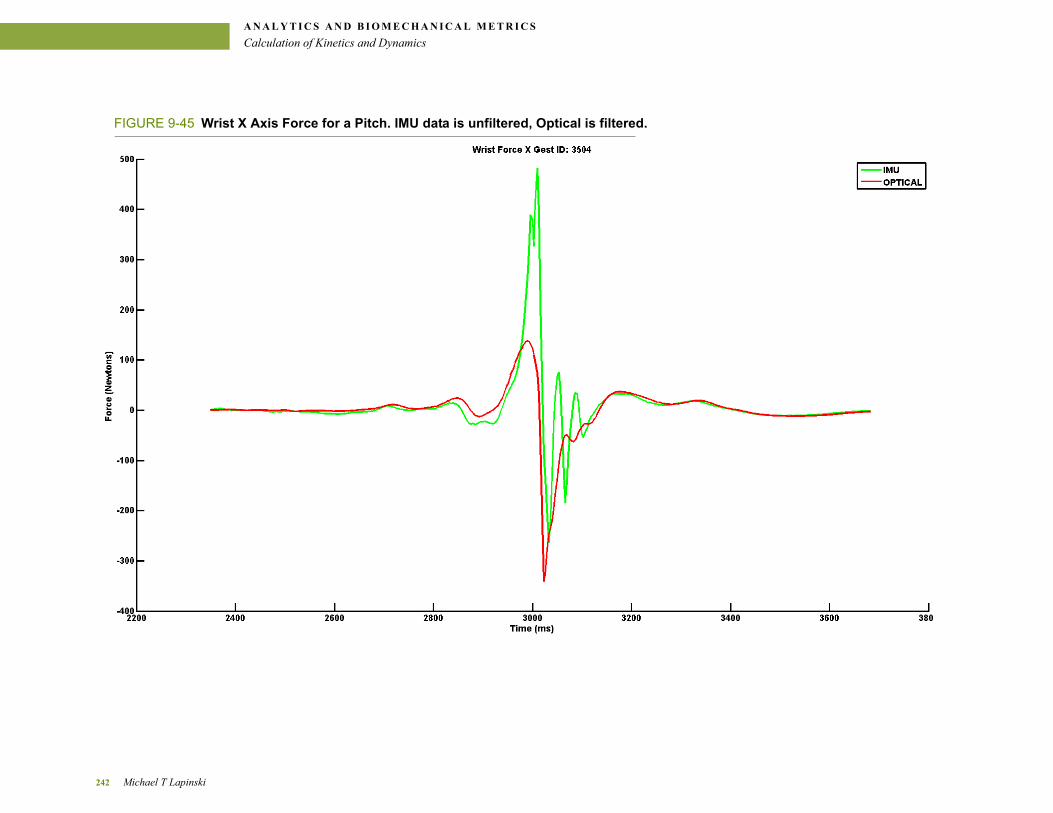
A N A L Y T I C S A N D B I O M E C H A N I C A L M E T R I C S
Calculation of Kinetics and Dynamics
FIGURE 9-45 Wrist X Axis Force for a Pitch. IMU data is unfiltered, Optical is filtered.
242 Michael T Lapinski
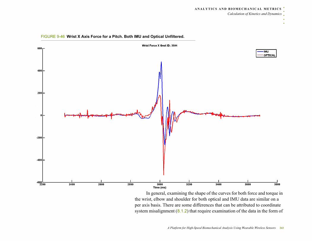
. . .
. .A N A L Y T I C S A N D B I O M E C H A N I C A L M E T R I C S
Calculation of Kinetics and Dynamics
FIGURE 9-46 Wrist X Axis Force for a Pitch. Both IMU and Optical Unfiltered.
In general, examining the shape of the curves for both force and torque in the wrist, elbow and shoulder for both optical and IMU data are similar on a per axis basis. There are some differences that can be attributed to coordinate system misalignment (8.1.2) that require examination of the data in the form of
A Platform for High-Speed Biomechanical Analysis Using Wearable Wireless Sensors 243
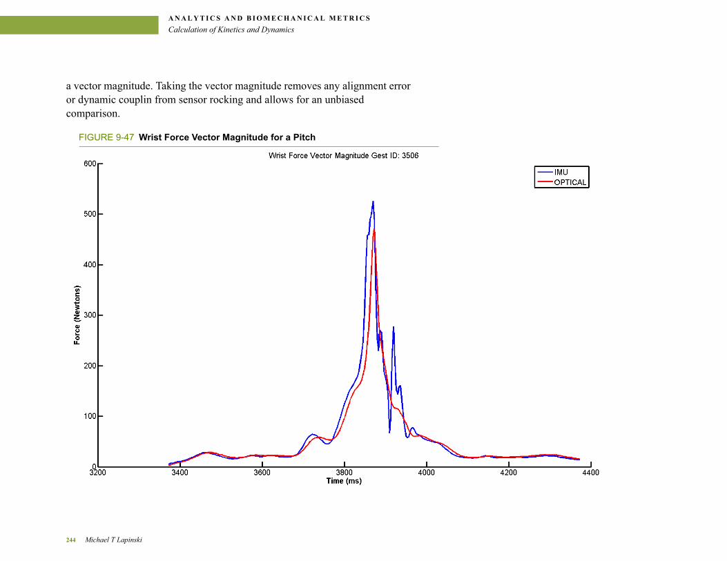
A N A L Y T I C S A N D B I O M E C H A N I C A L M E T R I C S
Calculation of Kinetics and Dynamics
a vector magnitude. Taking the vector magnitude removes any alignment error or dynamic couplin from sensor rocking and allows for an unbiased comparison.
FIGURE 9-47 Wrist Force Vector Magnitude for a Pitch
244 Michael T Lapinski
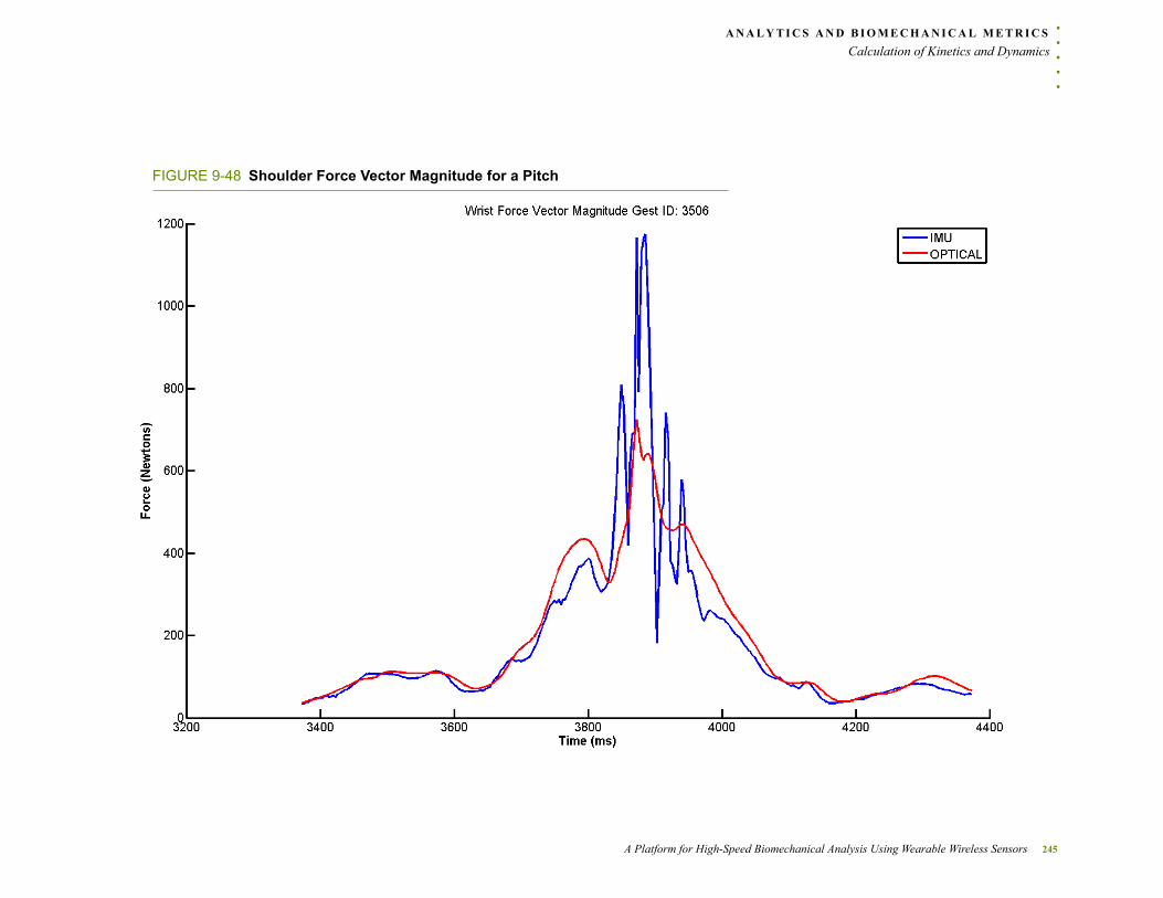
. . .
. .A N A L Y T I C S A N D B I O M E C H A N I C A L M E T R I C S
Calculation of Kinetics and Dynamics
FIGURE 9-48 Shoulder Force Vector Magnitude for a Pitch
A Platform for High-Speed Biomechanical Analysis Using Wearable Wireless Sensors 245
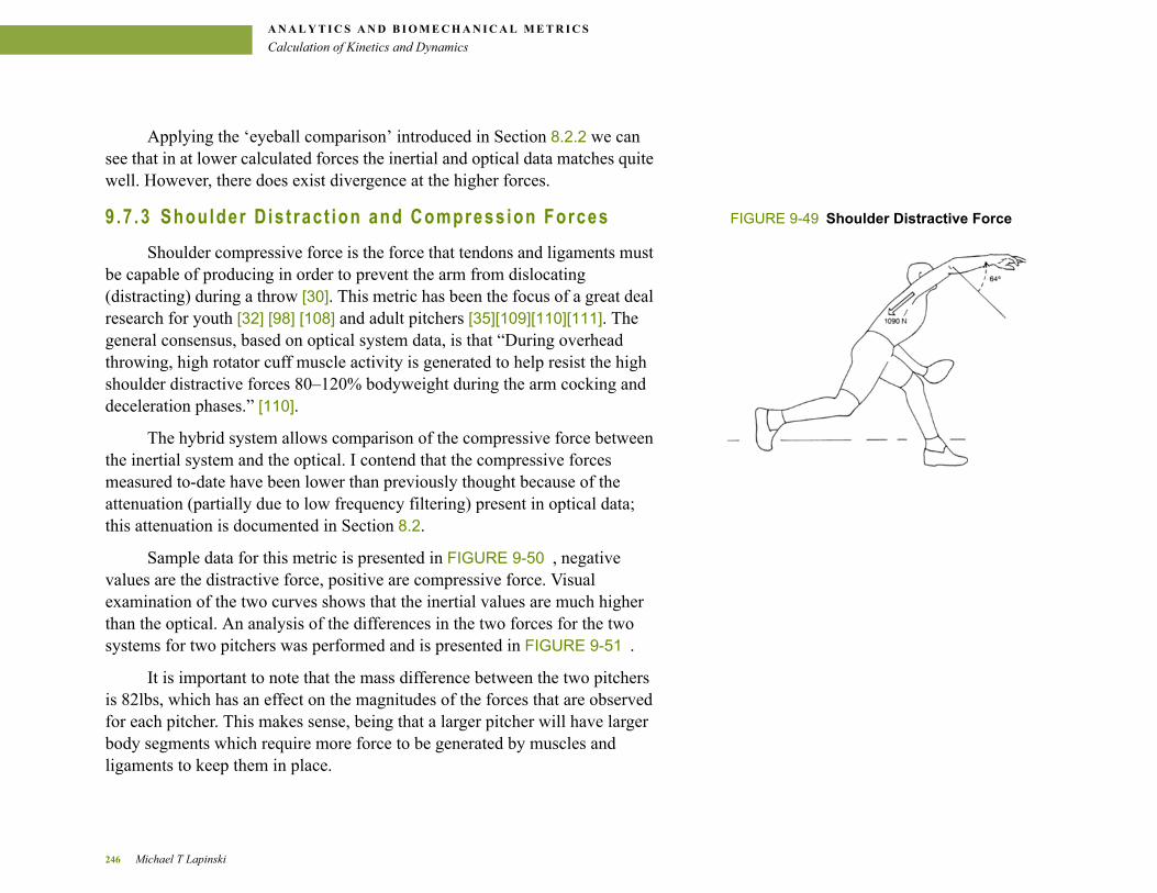
A N A L Y T I C S A N D B I O M E C H A N I C A L M E T R I C S
Calculation of Kinetics and Dynamics
Applying the ‘eyeball comparison’ introduced in Section 8.2.2 we can see that in at lower calculated forces the inertial and optical data matches quite well. However, there does exist divergence at the higher forces.
FIGURE 9-49 Shoulder Distractive Force 9 .7 .3 Shoulder D is t ract ion and Compress ion Forces
Shoulder compressive force is the force that tendons and ligaments must be capable of producing in order to prevent the arm from dislocating (distracting) during a throw [30]. This metric has been the focus of a great deal research for youth [32] [98] [108] and adult pitchers [35][109][110][111]. The general consensus, based on optical system data, is that “During overhead throwing, high rotator cuff muscle activity is generated to help resist the high shoulder distractive forces 80–120% bodyweight during the arm cocking and deceleration phases.” [110].
The hybrid system allows comparison of the compressive force between the inertial system and the optical. I contend that the compressive forces measured to-date have been lower than previously thought because of the attenuation (partially due to low frequency filtering) present in optical data; this attenuation is documented in Section 8.2.
Sample data for this metric is presented in FIGURE 9-50 , negative values are the distractive force, positive are compressive force. Visual examination of the two curves shows that the inertial values are much higher than the optical. An analysis of the differences in the two forces for the two systems for two pitchers was performed and is presented in FIGURE 9-51 .
It is important to note that the mass difference between the two pitchers is 82lbs, which has an effect on the magnitudes of the forces that are observed for each pitcher. This makes sense, being that a larger pitcher will have larger body segments which require more force to be generated by muscles and ligaments to keep them in place.
246 Michael T Lapinski
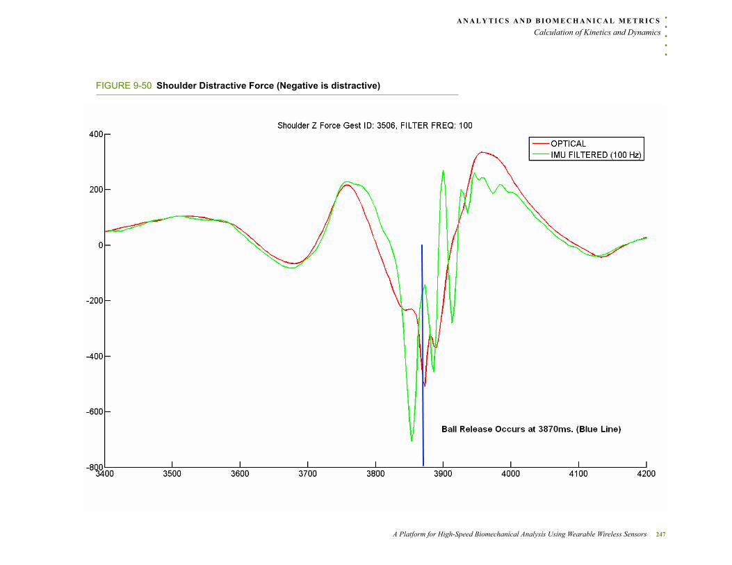
. . .
. .A N A L Y T I C S A N D B I O M E C H A N I C A L M E T R I C S
Calculation of Kinetics and Dynamics
FIGURE 9-50 Shoulder Distractive Force (Negative is distractive)
A Platform for High-Speed Biomechanical Analysis Using Wearable Wireless Sensors 247
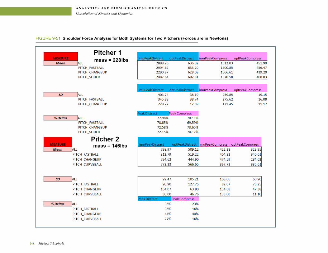
A N A L Y T I C S A N D B I O M E C H A N I C A L M E T R I C S
Calculation of Kinetics and Dynamics
FIGURE 9-51 Shoulder Force Analysis for Both Systems for Two Pitchers (Forces are in Newtons)
248 Michael T Lapinski
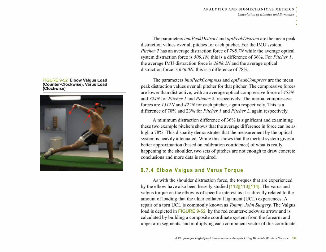
. . .
. .A N A L Y T I C S A N D B I O M E C H A N I C A L M E T R I C S
Calculation of Kinetics and Dynamics
The parameters imuPeakDistract and optPeakDistract are the mean peak distraction values over all pitches for each pitcher. For the IMU system, Pitcher 2 has an average distraction force of 798.7N while the average optical system distraction force is 509.1N; this is a difference of 36%. For Pitcher 1, the average IMU distraction force is 2888.2N and the average optical distraction force is 636.0N, this is a difference of 78%.
FIGURE 9-52 Elbow Valgus Load (Counter-Clockwise), Varus Load (Clockwise)
The parameters imuPeakCompress and optPeakCompress are the mean peak distraction values over all pitcher for that pitcher. The compressive forces are lower than distractive, with an average optical compressive force of 452N and 324N for Pitcher 1 and Pitcher 2, respectively. The inertial compressive forces are 1512N and 422N for each pitcher, again respectively. This is a difference of 70% and 23% for Pitcher 1 and Pitcher 2, again respectively.
A minimum distraction difference of 36% is significant and examining these two example pitchers shows that the average difference in force can be as high a 78%. This disparity demonstrates that the measurement by the optical system is heavily attenuated. While this shows that the inertial system gives a better approximation (based on calibration confidence) of what is really happening to the shoulder, two sets of pitches are not enough to draw concrete conclusions and more data is required.
9 .7 .4 E lbow Va lgus and Varus Torque
As with the shoulder distraction force, the torques that are experienced by the elbow have also been heavily studied [112][113][114]. The varus and valgus torque on the elbow is of specific interest as it is directly related to the amount of loading that the ulnar collateral ligament (UCL) experiences. A repair of a torn UCL is commonly known as Tommy John Surgery. The Valgus load is depicted in FIGURE 9-52 by the red counter-clockwise arrow and is calculated by building a composite coordinate system from the forearm and upper arm segments, and multiplying each component vector of this coordinate
A Platform for High-Speed Biomechanical Analysis Using Wearable Wireless Sensors 249
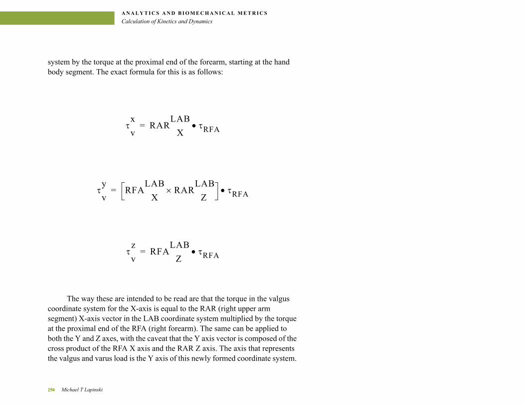
A N A L Y T I C S A N D B I O M E C H A N I C A L M E T R I C S
Calculation of Kinetics and Dynamics
system by the torque at the proximal end of the forearm, starting at the hand body segment. The exact formula for this is as follows:
x
vRAR
LAB
XRFA=
y
vRFA
LAB
XRAR
LAB
Z RFA=
z
vRFA
LAB
ZRFA=
The way these are intended to be read are that the torque in the valgus coordinate system for the X-axis is equal to the RAR (right upper arm segment) X-axis vector in the LAB coordinate system multiplied by the torque at the proximal end of the RFA (right forearm). The same can be applied to both the Y and Z axes, with the caveat that the Y axis vector is composed of the cross product of the RFA X axis and the RAR Z axis. The axis that represents the valgus and varus load is the Y axis of this newly formed coordinate system.
250 Michael T Lapinski

. . .
. .A N A L Y T I C S A N D B I O M E C H A N I C A L M E T R I C S
Calculation of Kinetics and Dynamics
Published values for valgus torque are 50±29 Nm [112]. For varus torque, published values range from 82±13 Nm [113] to 55±12 Nm [114]. In order to compare the output of the inertial and optical systems, the same style of analysis that was performed for shoulder distraction force for the same two pitchers using valgus and varus torque. Results from this analysis are presented in FIGURE 9-53 .
A Platform for High-Speed Biomechanical Analysis Using Wearable Wireless Sensors 251
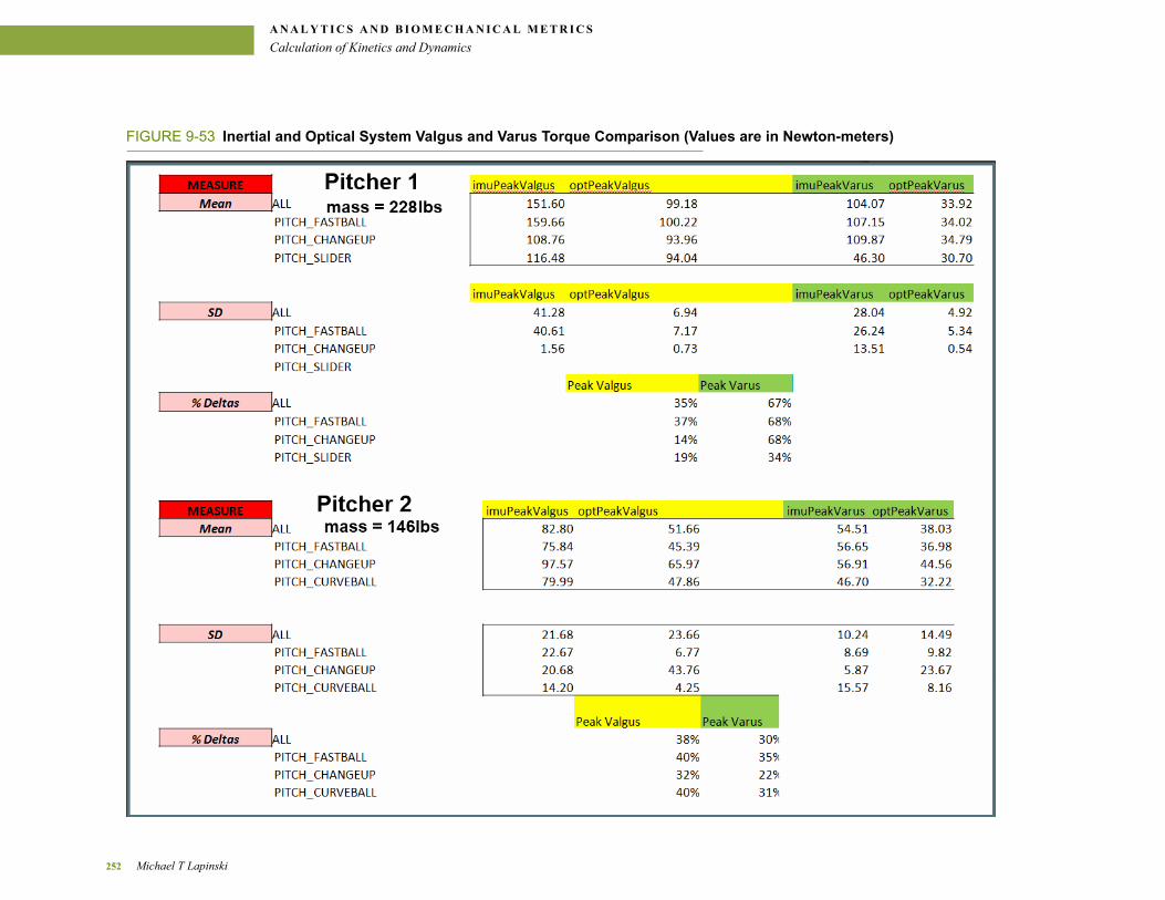
A N A L Y T I C S A N D B I O M E C H A N I C A L M E T R I C S
Calculation of Kinetics and Dynamics
FIGURE 9-53 Inertial and Optical System Valgus and Varus Torque Comparison (Values are in Newton-meters)
252 Michael T Lapinski
. . .
. .A N A L Y T I C S A N D B I O M E C H A N I C A L M E T R I C S
Calculation of Kinetics and Dynamics
As with the shoulder distraction force, the torques are higher for the larger pitcher. For the Pitcher 1 the mean valgus torque was 151.6Nm and 99.2Nm for the inertial and optical systems, respectively. Pitcher 2’s values are 82.8Nm and 51.7Nm, respectively. While the actual values are quite different, the amount of attenuation, in terms of a percentage, between the Pitcher 1 and Pitcher 2 are 35% and 38%.
Mean varus load for Pitcher 1 is 104.1Nm, inertial, and 34.0Nm, optical, and for Pitcher 2 54.6Nm, inertial, and 38.0Nm, optical. In percentages, these differences are 67% and 30%, with the larger disparity being for the player who has more mass.
As with previous metrics that utilize inertial data, the high confidence in calibration is used to state that the inertial-based data is consider to be more accurate. Based on this limited dataset, I can confidently state that the previously calculated optical system elbow torques fall at least 30% short and that the stress on the elbow is much greater than previously thought.
9 .7 .5 The F ine Pr in t
There are means through which the node attachment to the arm could artificially increase the measured peak value. For example, the mechanical characteristics of skin appear to be fairly compliant and soft until the skin is displaced maximally, where the displacement encounters rapid resistance forming something of a “hard stop”. In the course of a rapid motion, the node could be forced against the stop, experiencing large deceleration encountered by the node but not the arm. Additionally, if the node attachment is mechanically resonant, it could experience overshoot in response to a physical impulse as seen in a pitch. Such resulting ambiguities need to be explained in future measurements and simulations of the arm-node attachment and soft tissue dynamics.
A Platform for High-Speed Biomechanical Analysis Using Wearable Wireless Sensors 253

A N A L Y T I C S A N D B I O M E C H A N I C A L M E T R I C S
Calculation of Kinetics and Dynamics
254 Michael T Lapinski
. . .
. .C O N T R I B U T I O N S & C O N C L U S I O N S
CONTRIBUTIONS &
. . . .
. . . . . . . . . . . . . . . . . . . . . . . . . . . . . . . . . . . . . .CONCLUSIONS
A ll good things must come to an end.
- Thornton Wilder
This chapter summarizes the contributions and advancements in the state-of-art that this thesis has provided. It also presents new directions for continuing this work and challenges that will be faced by those attempting to push further.
A Platform for High-Speed Biomechanical Analysis Using Wearable Wireless Sensors 255

C O N T R I B U T I O N S & C O N C L U S I O N S
Contributions
. . . . . . . . . . . . . . . . . . . . . . . . . . . . . . . . . . . . . . . . . . . . . . . . . . . . . . . . . . .1 0 . 1 C O N T R I B U T I O N S
This thesis presents a novel end-to-end research platform that extends the capabilities of current biomechanical analysis.
The inertial measurement unit (IMU) network and hardware developed to enable measurement of the extreme forces is the only wearable IMU array that is capable of obtaining these measurements currently in existence. It has been designed to be robust to extreme activity and has been proven, because of rigorous calibration, to be a scientific tool accurate enough to perform life sciences quality research that brings more confidence to biomechanical analysis. By sampling at 1000Hz, it addresses the aliasing problem. With the developed rapid application system, it fits into the athletic workflow smoothly and increases the throughput of how much data can be gathered; unlike optical systems my IMU array can be easily deployed anywhere. Lastly, by leveraging the precision of inertial sensors the IMU system allows for the introduction of a new biomechanically relevant, never before considered, metric, jerk.
The platform allows clinical researchers to focus on research topics that are of interest to them and does require any sensor network or inertial sensing expertise in order to leverage the capabilities of the system. It provides a true end-to-end solution with graphical user interfaces, that abstract away the details of such systems, for every step of the process.
These interfaces start with network command and control, continue onto translation of gathered data into biomechanically relevant parameters (G-forces and angular velocities). They handle synchronization of the network itself and with other systems, allowing for realization of a hybrid inertial/optical system that leverages the strengths of both systems. The next level of interface integrates with an industry standard kinetics engine and allows feeding of more accurate inertial data into the kinetics algorithms. This
256 Michael T Lapinski
. . .
. .C O N T R I B U T I O N S & C O N C L U S I O N S
Contributions
integration provides clinically relevant inertial-based biomechanical metrics and provides the only existing mechanism for checking, and extending, the current accuracy of existing optical systems.
As part of the platform, a Player, Session and Gesture taxonomy and its underlying data model has been invented and realized. This provides a generic biomechanical data model that captures all the information needed for storing inertial information and all associated metadata for any physical activity. Due to this data-centric approach the system scales from tens to tens of thousands of gesture without any additional work. Further, application programming interfaces have been developed, in several computer programming languages, to allow access to this model in a language and platform independent manner. They allow for a query-based approach for defining clinical research populations based on any of the metadata parameters, such as pitch type or age or weight, that are enumerated in the data model.
The entire platform has been proven to work and is considered by experts in the field as “the future of motion capture”.
The system has been used to perform novel biomechanical measurements, (i.e. shoulder and elbow forces and torques, jerk forces, shoulder internal rotation, etc.) and have shown indications that widely accepted force/torque magnitudes in baseball pitching are consistently larger than previously work has shown.
A Platform for High-Speed Biomechanical Analysis Using Wearable Wireless Sensors 257

C O N T R I B U T I O N S & C O N C L U S I O N S
Future Work
. . . . . . . . . . . . . . . . . . . . . . . . . . . . . . . . . . . . . . . . . . . . . . . . . . . . . . . . . . .1 0 . 2 F U T U R E W O R K
10.2 .1 D i f fe rent ia t ion Between Rea l Mot ion & Sof t T issue Ar t i fac ts
As explained in Section 9.7.2, there are unexplained oscillations that are present in the unfiltered inertial data that appear to also be present in the unfiltered optical data. These oscillations have not been previously considered, because the low-frequency filtering of optical data removed them. A need exists to determine if they are real motion that is part of the pitch, or soft tissue artifacts. Soft tissue mounting could also affect the peak values of measured acceleration and rate and dynamic rocking of the IMU on the skin can couple axes. Soft tissue artifacts are covered in Section 8.1.3, which explains that the established way to answer this question is to surgically implant bone pins, or pursue the new research area of studying the effects of high linear acceleration on human skin when inertial nodes are fixed to it through a combination of mathematical modeling, simulation and actual measurement.
10 .2 .2 Coord inate System Al ignment Protocols
The pitfalls of coordinate system misalignment are described in Section 8.1.2. While this problem has not yet been solved, as part of this thesis initial steps were taken to characterize misalignment. A common coordinate system between the optical and inertial system has been defined at the Massachusetts General Hospital Sports Performance Center and some initial data has been gathered. Carolina Brum Medeiros, a callaborator from McGill University, has begun to define a gesture taxonomy to dynamically calculate the orientation misalignment angles for each node and her work is currently ongoing.
258 Michael T Lapinski
. . .
. .C O N T R I B U T I O N S & C O N C L U S I O N S
Future Work
10 .2 .3 Jo in t Angles
The next logical step in the current hybrid system is to remove the optical portion and calculate the joint angles using the standalone inertial system to drive the skeletal model. This is conventionally done by integrating the gyroscope signals using a Kalman Filter, getting initial angles and nulling offsets/noise via “ground sensor truth” from the magnetometer. This was attempted and the results were only partially successful. However, there are some difficult issues that need to be addressed in order to realize this system.
The first of these is the orientation representation system for each of the joint angles between body segments that was required to bring them into Visual3D. Visual3D required that each orientation be represented as an Euler angle. Euler angles suffer from gimbal lock, when two axes are rotated into the same plane, and it cannot be determined which axis is which. In order to deal with these singularities there are different angle application schemes (such as ZXZ) that require tracking of each angle over time, detecting and working around any gimbal lock that occurs. While these singularities are not a problem for Visual3D, they are a problem for the external algorithms that were developed to compute joint angles (using inertial data) outside of the Visual3D environment.
Clinically-defined research models prefer a particular set of coordinate systems. The inertial system prioritizes the comfort of the instrumented players and uses the best placement to avoid skin tissue artifacts. These two coordinate systems are not aligned and require transcription of initial angles from the inertial node coordinate system to the clinical coordinate system. Implementation of this transcription is not only a rotation, but also a change of basis.
Initial segment orientation relies heavily on fusion of magnetometer and low range accelerometer data. These algorithms were developed during the course of this thesis, unfortunately indoor magnetometer data in practice has
A Platform for High-Speed Biomechanical Analysis Using Wearable Wireless Sensors 259
C O N T R I B U T I O N S & C O N C L U S I O N S
Future Work
shown to be inaccurate and there is another level of (better) calibration required to obtain accurate initial orientation.
Assuming accurate enough initial orientation information, tracking the orientation of an individual segment over time via a Kalman filter has been shown to be feasible [63]. Additionally, the next step is to build a second level of Kalman filtering to determine the joint angle by building an estimator that uses the orientations of two nodes to observe a joint center. This leverages algorithms that are used by GPS satellite tracking, and no previously built wearable systems do this, as they simply assume a quaternion representation of each segment and calculate a joint angle based on the difference between the two quaternions. This approach is not sufficiently accurate in order to perform life sciences quality research.
10 .2 .4 Lower Cost Hybr id Systems
As optical capture technology has continually evolved since its inception, so has the cost of purchasing such a system. The faster the motion, the more cameras, with higher framerates, that are required to capture as much information as possible. A 500Hz system with enough cameras to capture pitching comes at a cost in the hundreds of thousands of dollars.
One hypothesis is that a high-end optical system isn't needed if it is complemented by an inertial network. Considering a hybrid inertial and optical system running at 100Hz, the hardware necessary to realize such a system is much cheaper to build than its high-end counterpart. An interesting question is how well would such a system work? While the aliasing problem would still exist, the accuracy of the sensors and their ability to provide high-quality inertial parameters would definitely help provide better data than a standalone optical system running at 100Hz, and help to properly interpolate the optical results.
260 Michael T Lapinski

. . .
. .C O N T R I B U T I O N S & C O N C L U S I O N S
Future Work
While the quality would not be that of the high-end system, such a low-cost system creates a market that would make it tractable for enable smaller organizations, such as little league teams, to perform biomechanically relevant motion capture.
10 .2 .5 Cont inued Data Acquis i t ion
The final piece of future work involves building a large body of data from various populations and various sports. Adding a layer of data mining on top of such a body of data would exploit the full power of the data-centric approach along with the full power of the inertial system to enable fine grained clinical research to draw more accurate conclusions and performance and injury predictions than previously has been possible.
A Platform for High-Speed Biomechanical Analysis Using Wearable Wireless Sensors 261

C O N T R I B U T I O N S & C O N C L U S I O N S
Future Work
262 Michael T Lapinski

. . .
. .
. . . .
. . . . . . . . . . . . . . . . . . . . . . . . . . . . . . . . . . . . . .REFERENCES
The References chapter provides the bibliographic information cross-referenced to the text.
MTL Thesis Title 263

[1] The Computer for the 21st Century. Mark Weiser. Scientific American, September 1991. Pgs 94-104.
[2] Body sensor networks for baseball swing training. Ghasemzadeh, H. and Jafari, R. 2010. Pervasive Computing and Communications Workshops. pp. 792-795.
[3] Roetenberg, D. Slycke, P. J. Veltink, P. H. Ambulatory position and orientation tracking fusing magnetic and inertial sensing. In Biomedical Engineering, IEEE Transactions on, pages 883 { 890, May 2007.
[4] Xsens Technologies B.V. Xsens motion technologies. http://www.xsens.com.
[5] Animazoo UK Ltd, Animazoo Motion Capture, http://www.animazoo.com/products
[6] Great Lakes Neurotechnologies, KinetiSense Motion Capture, http://www.glneurotech.com/KinetiSense/, http://glneurotech.com/support/brochures/kinetisense.pdf
[7] Lapinski, M., A Wearable, Wireless Sensor System for Sports Medicine, 2008, Masters Thesis, MIT Media Lab
[8] Vicon MotionSystems. Polygon. [Online] http://www.vicon.com/products/documents/Polygon4.pdf
[9] Jarrett MO, Andrews BJ, Paul JP. A television–computer system for the analysis of human locomotion, in: I.E.R.E. Golden Jubilee Conference. An exhibition on Application of Electronics in Medicine. Southampton University, Southampton, England, 1976.
[10] Qualisys Motion Capture Systems. [Online] , http://www.qualisys.com/products/
264 Michael T Lapinski

. . .
. .
[11] Fleisig, Glenn, Escamilla, Rafael and Andews, James. Biomechanics of Throwing. [book auth.] James E. Zachazewski and David J Magee. Athletic Injuries and Rehabilitation. s.l. : Saunders, 1996.
[12] Implications for the Development of Proximal Humeral Epiphysiolysis and Humeral Retrotorsion. Michelle B. Sabick, PhD, Young-Kyu Kim, MD, Michael R. Torry, PhD,. 11, s.l. : The American Journal of Sports Medicine , 2005, Vol. 33.
[13] McFarland, J. (1990). Coaching pitchers. Champaign, Ill: Leisure Press.
[14] Kindall, J., & Winkin, J. (2000). The baseball coaching bible. Champaign, IL: Human Kinetics.
[15] ST Microelectronics. (2008). Application Note AN2768: LIS331DL 3-axis digital MEMS accelerometer: translates finger taps into actions. http://www.st.com/st-web-ui/static/active/en/resource/technical/document/application_note/CD00196199.pdf
[16] Vicon Motion systems. T-Series Camera Documentation. (2010). http://www.vicon.com/products/documents/TSeriesSedition.pdf
[17] Zoopraxiscope. Wikipedia. [Online] 12 31, 2005. [Cited: 11 11, 2011.] http://en.wikipedia.org/wiki/Zoopraxiscope.
[18] Rotoscoping. Wikipedia. [Online] Oct 14, 2003. [Cited: 11 11, 2011.] http://en.wikipedia.org/wiki/Rotoscoping.
[19] Edgerton, Harold E. Abrupt change of load on a synchronous machine. Cambridge, MA : MIT Thesis, 1927.
[20] Mocapture, Society. History of Motion Capture. Mocap History. [Online] 2011. [Cited: 11 11, 2011.] http://motioncapturesociety.org/resources/industry-history.
[21] A clinically viable electrogoniometer. Cousins, S J, Hannah, R E and Foort, J. Atlanta, GA : s.n., 1979. 2nd Annual International Conference on Rehabilitation Engineering.
MTL Thesis Title 265

[22] Toward a Language for Human Movement. Calvert, Thomas W. 1986, Computers and the Humanities, pp. 35-43.
[23] Linder, Wilfred. Digital Photogrammetry. s.l. : Springer, 2006.
[24] Wikipedia. Bob Sabiston . Wikipedia. [Online] May 10, 2006. [Cited: 11 27, 2011.] http://en.wikipedia.org/wiki/Bob_Sabiston.
[25] Sabiston, Walter Roberts. Extracting 3D motion from hand-drawn animated figures. Cambridge, MA : MIT Thesis, 1991.
[26] Intra-rater and inter-rater reliability of gait measurements with CODA mpx30 motion analysis system. Maynard, V, et al. 2003, Gait & Posture, pp. 59-67.
[27] Prakash: lighting aware motion capture using photosensing markers and multiplexed illuminators. Raskar, Ramesh, et al. 3, s.l. : ACM TRANSACTIONS ON GRAPHICS, 2007, Vol. 26.
[28] McFarland, Joe. Coaching Pitchers. Champaign, Ill: Leisure Press, 1990.
[29] Carroll, Will. Saving the Pitcher: Preventing Pitching Injuries in Modern Baseball. Chicago: Ivan R. Dee, 2004.
[30] Fleisig, Glenn, Escamilla, Rafael and Andews, James. Biomechanics of Throwing. [book auth.] James E. Zachazewski and David J Magee. Athletic Injuries and Rehabilitation. s.l. : Saunders, 1996.
[31] Implications for the Development of Proximal Humeral Epiphysiolysis and Humeral Retrotorsion. Michelle B. Sabick, PhD, Young-Kyu Kim, MD, Michael R. Torry, PhD,. 11, s.l. : The American Journal of Sports Medicine , 2005, Vol. 33.
[32] The Effect of Pitching Biomechanics on the Upper Extremity in Youth and Adolescent Baseball Pitchers. J. T. Davis, Orr Limpisvasti, Derrick Fluhme, Karen J. Mohr, Lewis A. Yocum, Neal S. ElAttrache and Frank W. Jobe. 8, s.l. : Sage, 2009, Vol. 37. 10.1177/0363546509340226.
266 Michael T Lapinski

. . .
. .
[33] Werner SL, Murray TA, Hawkins RJ, et al. Relationships between throwing mechanics and shoulder distraction in professional baseball pitchers. In American Journal of Sports Medicine, 2001.
[34] Tullos HS, King J. Throwing mechanism in sports. In Orthopedic Clinic of North America; 4, pages 709{720, 1973.
[35] Fleisig GS, Kingsley DS, Loftice JW, et al. Kinetic comparison among the fastball, curveball, change-up, and slider in collegiate baseball pitchers. In American Journal of Sports Medicine, 2005.
[36] Body sensor networks for baseball swing training. Ghasemzadeh, H. and Jafari, R. 2010. Pervasive Computing and Communications Workshops. pp. 792-795.
[37] Vadim Gerasimov. Swings That Think. http://vadim.oversigma.com/stt/bat.html
[38] Gerasimov, Vadim. Every sign of life. Cambridge: Massachusetts Institute of Technology, 2003. http://hdl.handle.net/1721.1/28776.
[39] Feltner ME: Kinematic and kinetic parameters of the shoulder joint during the overarm baseball throw. Masters thesis. Indiana University, Bloomington, Indiana, 1984
[40] Feltner ME, Dapena J: Three-dimensional interactions in a two-segment kinetic chain. Part I: General model. Int J Sport Biomech 5: 403–419, 1989
[41] Feltner ME, Dapena JJ: Dynamics of the shoulder and elbow joints of the throwing arm during a baseball pitch. Int J Sport Biomech 2: 235–259, 1986
[42] M.E. Feltner, J. Dapena, Segmental interactions affecting the flexion/extension motion of the elbow during fastball baseball pitching, Journal of Biomechanics, Volume 21, Issue 10, 1988, Page 869,
[43] Eugene J. Alexander, Thomas P. Andriacchi, Correcting for deformation in skin-based marker systems, Journal of Biomechanics, Volume 34, Issue 3, March 2001, Pages 355-361
MTL Thesis Title 267

[44] Hansen C., Honeine J., et al. Low-cost motion capture systems in practice. Computer Methods in Biomechanics and Biomedical Engineering, Vol. 15, Iss. sup1, 2012
[45] Helen Liu, Cathy Holt, Sam Evans, Accuracy and repeatability of an optical motion analysis system for measuring small deformations of biological tissues, Journal of Biomechanics, Volume 40, Issue 1, 2007, Pages 210-214
[46] C. Reinschmidt, A.J. van den Bogert, B.M. Nigg, A. Lundberg, N. Murphy, Effect of skin movement on the analysis of skeletal knee joint motion during running, Journal of Biomechanics, Volume 30, Issue 7, July 1997, Pages 729-732
[47] Markus Windolf, Nils Götzen, Michael Morlock, Systematic accuracy and precision analysis of video motion capturing systems—exemplified on the Vicon-460 system, Journal of Biomechanics, Volume 41, Issue 12, 28 August 2008, Pages 2776-2780
[48] Michael S. Andersen, Daniel L. Benoit, Michael Damsgaard, Dan K. Ramsey, John Rasmussen, Do kinematic models reduce the effects of soft tissue artefacts in skin marker-based motion analysis? An in vivo study of knee kinematics, Journal of Biomechanics, Volume 43, Issue 2, 19 January 2010, Pages 268-273
[49] Stephane Armand, Morgan Sangeux, Pierre Hoffmeyer, Richard Baker, Optimal markers’ placement on the thorax for clinical gait analysis—A preliminary study, Gait & Posture, Volume 30, Supplement 2, November 2009, Page S54
[50] Steven Stanhope, John Holden, John Orsini, Effect of Target Attachement Techniques on Estimates of Shank Skeletal Motion., Gait & Posture, Volume 2, Nr. , 1994. Page 58
[51] Inge Söderkvist, Per-Åke Wedin, Determining the movements of the skeleton using well-configured markers, Journal of Biomechanics, Volume 26, Issue 12, December 1993, Pages 1473-1477, ISSN 0021-9290, 10.1016/0021-9290(93)90098-Y.
268 Michael T Lapinski

. . .
. .
[52] T.-W. Lu, J.J. O’Connor, Bone position estimation from skin marker co-ordinates using global optimisation with joint constraints, Journal of Biomechanics, Volume 32, Issue 2, February 1999, Pages 129-134,
[53] Rita Stagni, Silvia Fantozzi, Angelo Cappello, Double calibration vs. global optimisation: Performance and effectiveness for clinical application, Gait & Posture, Volume 29, Issue 1, January 2009, Pages 119-122
[54] Cappello, A.; Stagni, R.; Fantozzi, S.; Leardini, A., "Soft tissue artifact compensation in knee kinematics by double anatomical landmark calibration: performance of a novel method during selected motor tasks," Biomedical Engineering, IEEE Transactions on , vol.52, no.6, pp.992,998, June 2005
[55] Yeadon, MR (1990) The simulation of aerial movement - I: The determination of orientation angles from film data, Journal of Biomechanics, 23, pp.59-66, ISSN: 0021-9290.
[56] Yeadon, MR (1990) The simulation of aerial movement - II: A mathematical inertia model of the human body, Journal of Biomechanics, 23, pp.67-74, ISSN: 0021-9290.
[57] Yeadon, MR (1990) The simulation of aerial movement - III: The determination of the angular momentum of the huma//n body, Journal of Biomechanics, 23, pp.75-83, ISSN: 0021-9290.
[58] Yeadon, MR, Atha, J, Hales, FD (1990) The simulation of aerial movement - IV: A computer simulation model, Journal of Biomechanics, 23, pp.85-89, ISSN: 0021-9290.
[59] A. Ahmadi , D. Rowlands, J. Daniel, (2010) Development of inertial and novel marker-based techniques and analysis for upper arm rotational velocity measurements in tennis., Journal of Sports Engineering, 8, pp179-188
[60] Shanshan Chen; Cunningham, C.L.; Lach, J.; Bennett, B.C., "Extracting Spatio-Temporal Information from Inertial Body Sensor Networks for Gait Speed Estimation," Body Sensor Networks (BSN), 2011 International Conference on , vol., no., pp.71,76, 23-25 May 2011
MTL Thesis Title 269
[61] Chun-Hao Wu; Yuan-Tse Chang; Yu-Chee Tseng, "On Optimization of Accelerometers Deployment for Human Posture Tracking," Body Sensor Networks (BSN), 2011 International Conference on , vol., no., pp.186,190, 23-25 May 2011
[62] Burchfield, R.; Venkatesan, S., "A Framework for Golf Training Using Low-Cost Inertial Sensors," Body Sensor Networks (BSN), 2010 International Conference on , vol., no., pp.267,272, 7-9 June 2010
[63] A. D. Young, M. J. Ling, and D. K. Arvind. 2007. Orient-2: a realtime wireless posture tracking system using local orientation estimation. In Proceedings of the 4th workshop on Embedded networked sensors (EmNets '07). ACM, New York, NY, USA, 53-57.
[64] Arvind D K and Bates C A, “The Speckled Golfer”, 3rd Int. Conf. on Body Area Networks, Tempe AZ, USA, IEEE March 13 - 17, 2008.
[65] Visual3D, C-Motion Inc.:Research in Biomechanics. https://www.c-motion.com/products/visual3d/
[66] Winter, David A., “Biomechanics and motor control of human movement” ,2009, Hoboken, N.J. : Wiley
[67] Phadke, V., Braman, J. P., LaPrade, R. F., & Ludewig, P. M. (January 01, 2011). Comparison of glenohumeral motion using different rotation sequences. Journal of Biomechanics, 44, 4, 700-705.
[68] International Shoulder Group, http://internationalshouldergroup.org/
[69] Polhemus Motion Tracking Technical Comparisons. Polhemus Motion Tracking. http://www.polhemus.com/polhemus_editor/assets/polhemus-motion-tracking-technical-comparisons.pdf
[70] Arvind, D. K.; Valtazanos, A., "Speckled Tango Dancers: Real-Time Motion Capture of Two-Body Interactions Using On-body Wireless Sensor Networks," Wearable and Implantable Body Sensor Networks, 2009. BSN 2009. Sixth International Workshop on , vol., no., pp.312,317, 3-5 June 2009
270 Michael T Lapinski

. . .
. .
[71] Nissen CW, Westwell M, Ounpuu S, Patel M, Tate JP, Pierz K, Burns JP, Bicos J., "Adolescent baseball pitching technique: a detailed three-dimensional biomechanical analysis." Med Sci Sports Exerc. 2007 Aug;39(8):1347-57.
[72] Aguinaldo AL, Buttermore J, Chambers H., “Effects of upper trunk rotation on shoulder joint torque among baseball pitchers of various levels.” J Appl Biomech. 2007 Feb;23(1):42-51.
[73] Ge Wu, Frans C.T. van der Helm, H.E.J. (DirkJan) Veeger, Mohsen Makhsous, Peter Van Roy, Carolyn Anglin, Jochem Nagels, Andrew R. Karduna, Kevin McQuade, Xuguang Wang, Frederick W. Werner, Bryan Buchholz, ISB recommendation on definitions of joint coordinate systems of various joints for the reporting of human joint motion—Part II: shoulder, elbow, wrist and hand, Journal of Biomechanics, Volume 38, Issue 5, May 2005, Pages 981-992, ISSN 0021-9290, 10.1016/j.jbiomech.2004.05.042.
[74] Ryan Aylward. Sensemble: A Wireless Inertial Sensor System for Interactive Dance and Collective Motion Analysis. Master's thesis, Media Laboratory, Massachusetts Institute of Technology, 2006
[75] Quotes by clarinettist Jack Brymer. [Online] http://thinkexist.com/quotes/jack_brymer/
[76] Nordic Semiconductor. nRF2401A Transceiver [Online] http://[76][76]www.nordicsemi.com/eng/Products/2.4GHz-RF/nRF2401A
[77] Silicon Laboratories C8051[Online] http://www.silabs.com/Support%20Documents/TechnicalDocs/C8051F320-Short.pdf
[78] Atmel EVK1101 Development Board [Online] http://www.atmel.com/tools/evk1101.aspx
[79] Atmel AVR32 UC3A3 Series Microcontrollers [Online] http://www.atmel.com/devices/AT32UC3A3256.aspx
[80] Serial Peripheral Interface Bus [Online] https://en.wikipedia.org/wiki/Serial_Peripheral_Interface_Bus
MTL Thesis Title 271

[81] I²C [Online] https://en.wikipedia.org/wiki/I%C2%B2C
[82] Atmel Software Framework [Online] http://www.atmel.com/tools/avrsoftwareframework.aspx?tab=documents
[83] Secure Digital Input/Output Specification [Online] https://www.sdcard.org/developers/overview/sdio/sdio_spec/Simplified_SDIO_Card_Spec.pdf
[84] Analog Devices ADXRS649 Gyroscope [Online] http://www.analog.com/en/mems-sensors/mems-gyroscopes/adxrs649/products/product.html
[85] Analog Devices AD7606 Analog-to-Digital Converter [Online] http://www.analog.com/en/mems-sensors/mems-gyroscopes/adxrs649/products/product.html
[86] Analog Devices ADXL377 3-Axis Analog Accelerometer [Online] http://www.analog.com/en/mems-sensors/mems-accelerometers/adxl377/products/product.html
[87] Invensense IMU-3000 3-Azis Gyroscope [Online] http://www.invensense.com/mems/gyro/imu3000.html
[88] Analog Devices ADXL345 3-Axis digital Accelerometer [Online] http://www.analog.com/en/mems-sensors/mems-inertial-sensors/adxl345/products/product.html
[89] Honeywell 3-Axis Digital Compass [Online] http://www51.honeywell.com/aero/common/documents/myaerospacecatalog-documents/Defense_Brochures-documents/HMC5843.pdf
[90] Direct Memory Access [Online} https://en.wikipedia.org/wiki/Direct_memory_access
[91] Clemens Satzger. Fusion of Six-Dimensional Sensor Data Using Physics Engines (Diplom - TU München) January 2010.
272 Michael T Lapinski
. . .
. .
[92] Silicon Labs USB eXpress Application Programmers Interface [Online] http://www.silabs.com/products/mcu/Pages/USBXpress.aspx
[93] libusb-win32 USB Library [Online] http://sourceforge.net/apps/trac/libusb-win32/wiki
[94] Hirashima M. Induced acceleration analysis of three-dimensional multi-joint movements and its application to sports movements. In: Theoretical Biomechanics, V. Klika, ed. (InTech), pp. 303-318, 2011.
[95] Hirashima M, Yamane K, Nakamura Y, and Ohtsuki T. Kinetic chain of overarm throwing in terms of joint rotations revealed by induced acceleration analysis. Journal of Biomechanics. 41 (13):2874-2883, 2008.
[96] Hirashima M, Yamane K, Nakamura Y, and Ohtsuki T. Kinetic chain of overarm throwing in terms of joint rotations revealed by induced acceleration analysis. Journal of Biomechanics. 41 (13):2874-2883, 2008.
[97] Lafortune AM, Cavanagh RP. The measurement of normal knee joint motion during walking using intracortical pins. In: Whittle M, Harris D, eds. Biomechanical Measurements in Orthopaedic Practice . Oxford, U.K.: Clarendon; 1985;234–243.
[98] Effect of Pitch Type, Pitch Count, and Pitching Mechanics on Risk of Elbow and Shoulder Pain in Youth Baseball Pitchers. The American Journal of Sports Medicine 30 (4): 463-468, 200
[99] The Filthiest Pitches in Baseball, Blake Murphy, Oct 17 2012, [Online] http://www.beyondtheboxscore.com/2012/10/17/3514442/MLB-best-pitches-ranked-filthy-dickey-kershaw-darvish
[100] Werner SL, Murray TA, Hawkins RJ, et al. Relationships between throwingmechanics and shoulder distraction in professional baseball pitchers. In AmericanJournal of Sports Medicine, 2001.
[101] Fleisig GS, Kingsley DS, Loftice JW, et al. Kinetic comparison among the fastball,curveball, change-up, and slider in collegiate baseball pitchers. In American Journal of Sports Medicine, 2005.
MTL Thesis Title 273
[102] Berkson E., Aylward R., Zachazewski J., Paradiso J., Gill T.J. Imu arrays: Thebiomechanics of baseball pitching. In The Orthopaedic Journal at Harvard Medical School, Vol. 8, pages 90{94, June 2007.
[103] Dillman CJ, Fleisig GS, Andrews JR. Biomechanics of pitching with emphasis upon shoulder kinematics. In Journal of Orthopedic Sports Physical Therapy, pages 402{408, Aug 1993.
[104] Wearable Wireless Sensing for Sports and Ubiquitous Interactivity, Lapinski, M., Feldmeier, M. and Paradiso, J.A., in 2011 IEEE SENSORS Conference, 2011.
[105] Dunn F., Parberry I., 3E Math Primer for Graphics and Game Development. Worldware Publishing. 2002
[106] Geen, John. Progress in Integrated Gyroscopes. IEEE PLANS 2004
[107] The Kinetic Chain: Strength and Conditioning of the Baseball Athlete. UConn Health Center [Online] http://uconnsportsmed.uchc.edu/injury/prevention/kinetic_chain.html
[108] Biomechanics of the Shoulder in Youth Baseball Pitchers: Implications for the Development of Proximal Humeral Epiphysiolysis and Humeral Retrotorsion, M. B. Sabick; American Journal of Sports Medicine 33(11):1716-1722 (2005)
[109] "Pitching Biomechanics as a Pitcher Approaches Muscular Fatigue During a Simulated Baseball Game", R. F. Escamilla; The American Journal of Sports Medicine 35(1):23-33 (2006)
[110] Shoulder Muscle Recruitment Patterns and Related Biomechanics during Upper Extremity Sports", Rafael F. Escamilla; Sports Medicine 39(7):569-590 (2009)
[111] Werner SL, Guido JA Jr, Stewart GW, McNeice RP, VanDyke T, Jones DG. Relationships between throwing mechanics and shoulder
274 Michael T Lapinski

. . .
. .
distraction in collegiate baseball pitchers. J Shoulder Elbow Surg. 2007;16(1):37-42.
[112] Arnel L. Aguinaldo and Henry Chambers. Correlation of Throwing Mechanics With Elbow Valgus Load in Adult Baseball Pitchers. Am J Sports Med 2009 37
[113] Fleisig GS, Barrentine SW, Zheng N, Escamilla RF, Andrews JR. Kinematic and kinetic comparison of baseball pitching among various levels of development. J Biomech. 1999;32:1371-1375.
[114] Fleisig GS, Kingsley, DS, Loftice,JW, Dinnen, KP, Andrews JR. et al. Kinetic Comparison Among the Fastball,Curveball, Change-up, and Slider in Collegiate Baseball Pitchers Am J Sports Med. 2006 Mar;34(3):423-30.
[115] Sensemble: A Wireless, Compact, Multi-User Sensor System for Interactive Dance, Ryan Aylward, and Joseph A. Paradiso, in Proc. of NIME 2006, The 2006 International Conference on New Interfaces for Musical Expression, Paris, France, June 4-8, 2006, pp. 134-139.
[116] Seinfeld Episode #104: “The Doorman” [Online] https://en.wikipedia.org/wiki/The_Doorman
MTL Thesis Title 275

276 Michael T Lapinski