FRANK M. MONALDO

A PRACTICAL METHODOLOGY FOR ESTIMATING WAVE SPECTRA FROM THE SIR-B

A step-by-step procedure is outlined to convert synthetic aperture radar imagery into estimates of ocean surface-wave s~ectra .. The ~rocedure is based on a linearized version of a model that relates synthetic apert~re ra~ar Image mt~nsity spectra and wave slope- or height-variance spectra. The outlined proce­dure IS applIed to synthetIc aperture radar imagery from the Shuttle Imaging Radar mission and is shown to produce spectra that, except in the lowest sea state, are highly correlated with two-dimensional spectra measured independently.

INTRODUCTION

A number of investigators have demonstrated the general resemblance of synthetic aperture radar (SAR) image spectra and ocean-wave spectra. 1-3 Within certain limits, the wavenumber (or inverse wavelength) and propagation direction of ocean-wave systems derived from SAR image spectra have agreed well with indepen­dent measures of these parameters.

A more complete verification of the potential of space­borne SARs to produce reliable wave-spectra estimates has awaited two developments: (a) alternative airborne techniques to estimate two-dimensional wave spectra with wavenumber and angular resolution comparable to those of SAR image spectra, and (b) an integration of various SAR wave-imaging theories into a procedure for converting SAR image spectra into estimates of ocean­wave slope- or height-variance spectra.

During the second Shuttle Imaging Radar (SIR-B) mis­sion in October 1984, SAR imagery was acquired off the southern coast of Chile. Simultaneously, two-dimen­sional wave spectra were acquired by a NASA P-3 air­craft equipped with a radar ocean-wave spectrometer (ROWS)4 and a surface contour radar (SCR). s Both instruments had been tested and verified in previous ex­periments.

In 1981, Alpers et al. 6 proposed a comprehensive ap­proach to the interpretation of SAR image modulation in terms of ocean surface wave slope. A linearized and simplified version of the wave-imaging models detailed by Alpers et al. (see the article by Lyzenga preceding this one) was included in a proposed method by Monaldo

82

Frank M. Monaldo is a senior staff phys­icist in the Space Geophysics Group, The Johns Hopkins University Applied Phys­ics Laboratory, Laurel, MD 20707.

and Lyzenga 7 to convert SAR wave imagery into esti­mates of ocean-wave slope- and height-variance spectra.

In this article, we will review a practical procedure for converting SAR imagery to wave spectra, particularly emphasizing some of its still-uncertain aspects. We will also compare SAR wave spectra computed using this procedure with spectra estimated independently from the ROWS and SCR, thereby revealing both the potential and the limitations of the SAR to estimate wave spec­tra. Additional spectral comparisons from the SIR-B ex­periment are discussed in the article by Beal in this issue. Some early comparisons are also given in Beal et al. 8

WAVE-SPECTRA ESTIMATION PROCEDURE

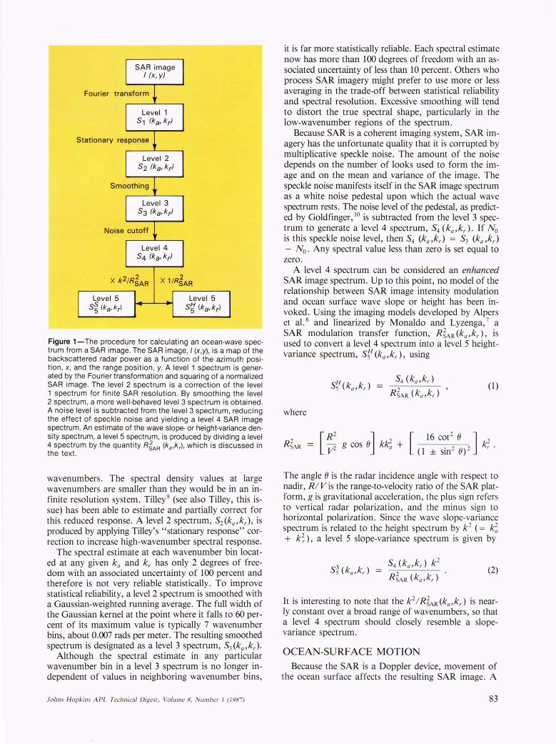
A five-step procedure used to estimate wave slope- and height-variance spectra is shown schematically in Fig. 1. 7 The initial input is the two-dimensional SAR inten­sity image I (x,y). When properly calibrated, image in­tensity is proportional to back scattered radar power. The digitally processed, geometrically and radiometrically corrected imagery used in this article has been provided by the Jet PropUlsion Laboratory. The imagery is divided into image frames 512 by 512 pixels on a side. Each pixel corresponds to an area 12.5 by 12.5 meters on the sur­face, so that the entire image frame covers a 6.4- by 6.4-kilometer area.

Image normalization is performed by subtracting the mean image intensity and then dividing by this mean. The resulting normalized image is in units of fractional modulation. SAR wave-imaging theories are generally characterized in terms of fractional image modulation.

Fourier transformation of the image and squaring re­sult in a level 1 spectrum, SI (ka,kr)' where ka is the az­imuth (parallel to the satellite track) wavenumber and kr is the range (perpendicular to the satellite track) wavenumber.

All imaging systems have finite resolution, and SARs are no exception. The effect of this finite resolution on SAR image spectra is to reduce spectral response at high

Johns H opkins A PL Technica l D igesi , Volum e 8, N um ber I (1 987)

Fourier

Level 5 S~ (ka,krl

2 X 11RSAR

Level 5 S~ (ka,kr )

Figure 1-The procedure for calculating an ocean-wave spec­trum from a SAR image. The SAR image, I (x,Y) , is a map of the backscattered radar power as a function of the azimuth posi­tion , x, and the range position , y. A level 1 spectrum is gener­ated by the Fourier transformation and squaring of a normalized SAR image. The level 2 spectrum is a correction of the level 1 spectrum for finite SAR resolution. By smoothing the level 2 spectrum, a more well-behaved level 3 spectrum is obtained. A noise level is subtracted from the level 3 spectrum, reducing the effect of speckle noise and yielding a level 4 SAR image spectrum. An estimate of the wave slope- or height-variance den­sity spectrum, a level 5 spectrum, is produced by dividing a level 4 spectrum by the quantity R~AR (ka ,k r), which is discussed in the text.

wavenumbers_ The spectral density values at -large wavenumbers are smaller than they would be in an in­finite resolution system. Tilley9 (see also Tilley, this is­sue) has been able to estimate and partially correct for this reduced response. A level 2 spectrum, 52 (ka,kr ), is produced by applying Tilley's "stationary response" cor­rection to increase high-wavenumber spectral response.

The spectral estimate at each wavenumber bin locat­ed at any given ka and kr has only 2 degrees of free­dom with an associated uncertainty of 100 percent and therefore is not very reliable statistically. To improve statistical reliability, a level 2 spectrum is smoothed with a Gaussian-weighted running average. The full width of the Gaussian kernel at the point where it falls to 60 per­cent of its maximum value is typically 7 wavenumber bins, about 0.007 rads per meter. The resulting smoothed spectrum is designated as a level 3 spectrum, 53 (ka,kr).

Although the spectral estimate in any particular wavenumber bin in a level 3 spectrum is no longer in­dependent of values in neighboring wavenumber bins,

Johns H opkins APL Technica l Digest, Volume 8. Number I (/987)

it is far more statistically reliable. Each spectral estimate now has more than 100 degrees of freedom with an as­sociated uncertainty of less than 10 percent. Others who process SAR imagery might prefer to use more or less averaging in the trade-off between statistical reliability and spectral resolution. Excessive smoothing will tend to distort the true spectral shape, particularly in the low-wavenumber regions of the spectrum.

Because SAR is a coherent imaging system, SAR im­agery has the unfortunate quality that it is corrupted by multiplicative speckle noise. The amount of the noise depends on the number of looks used to form the im­age and on the mean and variance of the image. The speckle noise manifests itself in the SAR image spectrum as a white noise pedestal upon which the actual wave spectrum rests. The noise level of the pedestal, as predict­ed by Goldfinger, 10 is subtracted from the level 3 spec­trum to generate a level 4 spectrum, 54 (ka, kr ). If N o is this speckle noise level, then 54 (ka ,kr) = 53 (ka ,kr) - N o. Any spectral value less than zero is set equal to zero.

A level 4 spectrum can be considered an enhanced SAR image spectrum. Up to this point, no model of the relationship between SAR image intensity modulation and ocean surface wave slope or height has been in­voked . Using the imaging models developed by Alpers et al. 6 and linearized by Monaldo and Lyzenga, 7 a SAR modulation transfer function, R~AR (ka,kr ), is used to convert a level 4 spectrum into a level 5 height­variance spectrum, 5f (ka,kr ), using

where

54 (ka, kr )

R~AR (ka,kr ) , (1)

[ R 2 ] [16 cot

2 e ] R~AR = 2 g cos e kk?; + . 2 2 k,.

V (1 ± sm e)

The angle e is the radar incidence angle with respect to nadir, R I V is the range-to-velocity ratio of the SAR plat­form, g is gravitational acceleration, the plus sign refers to vertical radar polarization, and the minus sign to horizontal polarization. Since the wave slope-variance spectrum is related to the height spectrum by k 2 (= k~ + k~ ), a level 5 slope-variance spectrum is given by

54 (ka, kr ) k 2

R~AR (ka, kr ) (2)

It is interesting to note that the k 2 I R~AR (ka, kr ) is near­ly constant over a broad range of wavenumbers, so that a level 4 spectrum should closely resemble a slope­variance spectrum.

OCEAN-SURFACE MOTION Because the SAR is a Doppler device, movement of

the ocean surface affects the resulting SAR image. A

83

Monaldo - Practical Methodology for Estimating Wave Spectra from the SfR-B

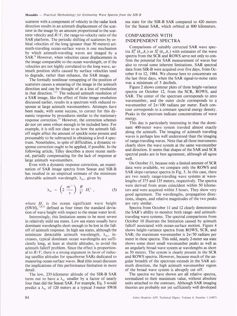
scatterer with a component of velocity in the radar look direction results in an azimuth displacement of the scat­terer in the image by an amount proportional to the scat­terer velocity and R/ V, the range-to-velocity ratio of the SAR platform. The periodic shifting of scatterers by or­bital velocities of the long (greater than 50 meters) azi­muth-traveling ocean-surface waves is one mechanism by which azimuth-traveling waves are imaged by a SAR. 6 However, when velocities cause displacements in the image comparable to the ocean wavelength, or if the velocities are not highly correlated to the long wave, az­imuth position shifts caused by surface velocities tend to degrade, rather than enhance, the SAR image.

The formally nonlinear remapping of the position of scatterers causes a smearing of the image in the azimuth direction and can be thought of as a loss of resolution in that direction. 7,11 The reduced azimuth resolution of a SAR image, like the effect of finite image resolution discussed earlier, results in a spectrum with reduced re­sponse at large azimuth wavenumbers. Attempts have been made, with some success, to correct for this dy­namic response by procedures similar to the stationary response correction. 11 However, the correction schemes do not yet seem robust enough to be included here. For example, it is still not clear to us how the azimuth fall­off might affect the amount of speckle noise present and presumably to be subtracted in obtaining a level 4 spec­trum. Nonetheless, in spite of difficulties, a dynamic re­sponse correction ought to be applied, if possible. In the following article, Tilley describes a more recent meth­od, partially compensating for the lack of response at large azimuth wavenumbers.

Even with a dynamic response correction, an exami­nation of SAR image spectra from Seasat and SIR-B has resulted in an empirical estimate of the minimum detectable azimuth wavelength, Am' given by

Am - 2 '!:!.- - H Vz ( VZ) R

s V s ' (3)

where Hs is the ocean significant wave height (SWH), 7,8,11 defined as four times the standard devia­tion of wave height with respect to the mean water level.

Interestingly, this limitation seems to be most severe in relatively mild sea states. Low sea states usually have dominant wavelengths short enough to be lost in the fall­off of azimuth response. In high sea states, although the minimum detectable azimuth wavelength, Am' in­creases, typical dominant ocean wavelengths are suffi­ciently long, at least at shuttle altitudes, to avoid the azimuth falloff problem. Since the effect is proportion­al to R / V, there is a strong argument in favor of reduc­ing satellite altitudes for spaceborne SARs dedicated to measuring ocean-surface waves. Beal (this issue) discusses the implications of this performance limitation in more detail.

The low, 235-kilometer altitude of the SIR-B SAR turns out to have a Am smaller by a factor of nearly four than did the Seasat SAR. For example, Eq. 3 would predict a Am of 120 meters at a typical 3-meter SWH

84

sea state for the SIR-B SAR compared to 420 meters for the Seas at SAR, which orbited at 800 kilometers.

COMPARISONS WITH INDEPENDENT SPECTRA

Comparisons of suitably corrected SAR wave spec­tra Sr (ka ,kr) or S~ (ka ,kr) with estimates of the wave spectra from the SCR and ROWS serve not only to con­firm the potential for SAR measurement of waves but also to reveal some inherent limitations. SAR spectral data from SIR-B were acquired over five days, from Oc­tober 8 to 12, 1984. We choose here to concentrate on the last three days, when the SAR signal-to-noise ratio was a minimum of 5 decibels.

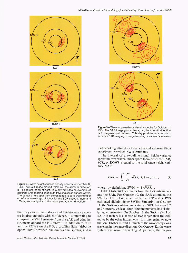
Figure 2 shows contour plots of three height-variance spectra on October 12, from the SCR, ROWS, and SAR. The center of the spectrum corresponds to zero wavenumber, and the outer circle corresponds to a wavenumber of 27r/ l00 radians per meter. Each con­tour corresponds to a constant spectral energy density. Peaks in the spectrum indicate concentrations of wave energy.

This day is particularly interesting in that the domi­nant 400-meter wave system traveled almost exactly along the azimuth. The imaging of azimuth traveling waves is perhaps less well understood than the imaging of range-traveling waves. Note that all three instruments clearly show the wave system at the same wavenumber and direction. It seems that shapes of the SAR and SCR spectral peaks are in best agreement, although all agree well.

On October 11, because only a limited amount of SCR data were available, we compare only the ROWS and SAR slope-variance spectra in Fig. 3. In this case, there are two nearly range-traveling wave systems at wave­lengths of 375 and 135 meters, respectively. The spectra were derived from areas coincident within 50 kilome­ters and were acquired within 3 hours. They show very good agreement. The wavelengths, propagation direc­tions, shapes, and relative magnitudes of the two peaks are very similar.

Spectra from October 11 and 12 clearly demonstrate the SAR's ability to monitor both range- and azimuth­traveling wave systems. The spectral comparisons from October 10 illustrate the limitation caused by azimuth falloff associated with ocean-surface motion. Figure 4 shows height-variance spectra from ROWS, SCR, and SAR; the maximum wavenumber is 27r/50 radians per meter in these spectra. This mild, nearly 2-meter sea state shows some short small wavenumber peaks as well as an angularly broad wave system at wavelengths as short as 50 meters. The system is clearly present in the SCR and ROWS spectra. However, because much of the an­gular breadth of the spectrum extends in the SAR azi­muth direction, the high azimuth wavenumber region of the broad wave system is abruptly cut off.

The spectra we have shown are all relative spectra, normalized to their maximum value, without absolute units attached to the contours. Although SAR imaging theories are probably not yet sufficiently well developed

Johns H opkins APL Technica l Digest, Volume 8, N um ber I (1987)

Monaldo - Practical Methodology for Estimating Wave Spectra from the SIR-B

SCR

Figure 2-Wave height-variance density spectra for October 12, 1984. The SAR image ground track, i.e. , the azimuth direction, is 11 degrees north of east. This day provides an example of accurate SAR imaging of azimuth-traveling ocean surface waves. The center of the spectrum corresponds to zero wavenumber or infinite wavelength . Except for the SCR spectra, there is a 180-degree ambiguity in the wave propagation direction.

that they can estimate slope- and height-variance spec­tra in absolute units with confidence, it is interesting to compare the SWH estimate from the SAR and other in­struments aboard the P-3 aircraft. In addition to SCR and the ROWS on the P-3, a profiling lidar (airborne optical lidar) provided one-dimensional spectra, and a

Johns H opkins A PL Technica l Digest , Volum e 8, Number I (/98 7)

ROWS

SAR

Figure 3-Wave slope-variance density spectra for October 11 , 1984. The SAR image ground track, i.e., the azimuth direction, is 11 degrees north of east. This day provides an example of accurate SAR imaging of range-traveling ocean-surface waves.

nadir-looking altimeter of the advanced airborne flight experiment provided SWH estimates.

The integral of a two-dimensional height-variance spectrum over wavenumber space from either the SAR, SCR, or ROWS is equal to the total wave height vari­ance VAR:

VAR = r r S~(k"k,) dk, dk, , (4)

where, by definition, SWH = 4 ~ _ Table 1 lists SWH estimates from the P-3 instruments

and the SAR. For October 10, the SAR estimated the SWH at 1.3 to 1.4 meters, while the SCR and ROWS estimated slightly higher SWHs_ Similarly, on October 11, the SAR modulation indicated an SWH between 3.2 and 4 meters, while all four other instruments had slight­ly higher estimates. On October 12, the SAR's SWH of 5.6 to 6 meters is a factor of two larger than the esti­mates by the other instruments. It is interesting to note that on October 10 and 11 much of the wave energy was traveling in the range direction. On October 12, the wave system was azimuth traveling. Apparently, the magni-

85

Monaldo - Practical Methodology for Estimating Wave Spectra from the SIR-B

ROWS

seR

SAR

Figure 4-Wave height-variance density spectra for October 10, 1984. The SAR image ground track, i.e., the azimuth direction, is 11 degrees north of east. Note that these spectra (in con­trast to Figs. 2 and 3) have a minimum displayed wavelength of 50 meters. Both the SeR and ROWS spectra show a very broad wave system whose dominant wavelength is about 70 meters. The SAR spectrum clearly exhibits a lack of response at high wavenumbers (shorter wavelengths) in the azimuth direc­tion. The result is that the angular width of the 70-meter wave­length system appears greatly reduced.

tude of the component of our model for R SAR (kpka )

in the azimuth direction is a factor of two too small. On the other hand, the range component of the model appears slightly too large.

86

Table 1-SWH comparisons (meters).

Aircraft Instruments Date

Shuttle SAR ROWS SCR AOL* AAFE**

October 10 1.3 to 1.4 1.9 October 11 3.2 to 4.0 4.6 October 12 5.6 to 6.0 3.3

* AOL = airborne optical lidar

1.7 4.1 3.3

4.4 3.7

4.6 3.5

* * AAFE = advanced airborne flight experiment (altimeter)

The fact that the SWH can be estimated this closely with SAR spectra is somewhat surprising and indicates that the linearized SAR imaging model is fairly good. Until we understand SAR modulation mechanisms more completely, relative SAR spectra will be more accurate­ly normalized with SWH estimates from a radar al­timeter.

CONCLUSIONS A specific procedure for estimating slope- and height­

variance spectra from SAR imagery has been developed and implemented that seems to produce relative spectra in close agreement with independently measured spec­tra. More work is required in specifying the exact mag­nitude of the SAR wave imaging function R§AR (ka,kr)'

The most important limitation in SAR wave imagery is the lack of response at large azimuth wavenumbers caused by ocean-surface motion. Although this prob­lem is partially correctable, low satellite orbits will be required to maximize the usefulness of ocean spectra de­rived from spaceborne SAR imagery.

REFERENCES

1 R. C. Beal , D . G. Tilley, and F. M. Monaldo, "Large- and Small-Scale Spa­tial Evolution of Digitally Processed Ocean Wave Spectra from the Seasat Syn­thetic Aperture Radar," 1. Geophys. Res. 88, 1761 -1778 (1983).

2 R. C. Beal, T. W. Gerling, D . E. Irvine, F. M. Monaldo, and D. G. Tilley, " Spatial Variations of Ocean Wave Directional Spectra from the Seasat Syn­thetic Aperture Radar," 1. Geophys. Res. 91, 2433-2449 (1986).

3 R. A. Shuchman, J. D. Lyden, and D. R. Lyzenga, " Estimates of Ocean Wavelength and Direction from X- and L-Band Synthetic Aperture Radar dur­ing the Marineland Experiment," IEEE J. Oceanic Eng. OE-8, 90-96 (1983) .

4 F . C. Jackson, W . T. Walton, and P. L. Baker, "Aircraft and Satellite Mea­surement of Ocean Wave Directional Spectra using Scanning-Beam Microwave Radars," J. Geophys. Res. 90, 987-1004 (1985) .

5 E. J. Walsh, D . W. Hancock 111 , D. E . Hines, R. . Swift , and J . F. SCOll, " Directional Wave Spectra Measured with the Surface Contour Radar," J. Phys. Oceanogr. 15, 566 (1985).

6 W . Alpers, D. B. Ross, and C. L. Rufenach , "On the Detectability of Ocean Surface Waves by Real and Synthetic Aperture Radar," 1. Geophys. Res. 86, 6481-6498 (1981) .

7 F. M . Monaldo and D. R. Lyzenga, "On the Estimation of Wave Siope- and Height-Variance Spectra from SAR Imagery," IEEE Trans. Geosci. Remote Sensing (in press, 1986).

8 R . C. Beal, F. M . Monaldo, D. G . Tilley, D. E. Irvine, E . J. Walsh, F. C. Jackson, D . W . Hancock III, D. E . Hines, R. . Swift, F. I. Gonzalez, D. R . Lyzenga, and L. F. Zambresky, "A Comparison of SIR-B Directional Wave Spectra with Aircraft Scanning Radar Spectra and Spectral Ocean Wave Model Predictions," Science 232, 1531-1535 (1986) .

9 D . G . Tilley, "Use of Speckle for Estimating Response Characteristics of Dop­pler Imaging Radars, " Opt. Eng. 25 , 772-779 (1986) .

10 A. D. Goldfinger, "Estimation of Spectra from Speckled Images," IEEE Trans. Aerosp. Electron. Syst. 18, 675-681 (1982).

11 F. M. Monaldo, " Improvement in the Estimate of Dominant Wavenumber and Direction from Spacebome SAR Image Spectra when Corrected for Ocean Surface Movement," IEEE Trans. Geosci. Remote Sensing GE-22, 603-608 (1984).

Johns H opkins APL Technical Digest, Volum e 8, Number J (1987)