A Profile of Crime in Long Beach Using ArcGIS

Spatial Statistics Tools

J. Chris CarterProfessor of GeographyLong Beach City College

Goals of Presentation

• Share my application of ArcGIS tools for crime analysis- Working with crime data- Crime counts and rates- Hotspot analysis- Regression analysis- Distance between crime-arrestee and crime-victim

Long Beach

Long Beach Demographics (2015)

• Population: 471,210• Diversity Index: 87.8• Per Capita Income: $25,807

- 86% of California per capita income

• Didn’t Finish High School: 9.0%- 110% of California’s rate

• Bachelor’s Degree: 18.6%- Same as California

• Renter Occupied Housing Units: 56%- 132% of California’s rate

• Data source: Esri Business Analyst

Crime Data

• Long Beach Police Department - 2010-2014

• Included:- Crime type- Crime location by address- Arrestee/Citee by address- Victim by address

Crime Data: Geocoding

• Tip #1:

• Use ArcGIS Desktop to geocode first. • Then use ArcGIS Online for the rest.

- Save credits that way.

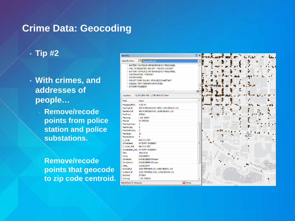
Crime Data: Geocoding

• Tip #2

• With crimes, and addresses of people…

- Remove/recode points from police station and police substations.

- Remove/recode points that geocode to zip code centroid.

Hotspot Analysis

• Consider Scale.- Block, neighborhood, city, or regional patterns?

- 1. Determine your units of analysis - Fishnet grid, census block groups, census tracts…

- 2. Determine your Distance Band- Larger band= broader patterns- Smaller band= local patterns

Hotspot Analysis: Effect of Distance Threshold

• Robbery Rate- 3000’ distance threshold vs. 12,000’ distance threshold- Both are statistically valid

Hotspot Analysis: Counts vs. Rates

• Crime counts- Useful for patrol officers and commanders.- Where are the crimes and where do I need more officers?

• Crime rates- Useful for researchers and policymakers.- Control for population size/housing units.- Where are a higher proportion of people involved in crimes?

Hotspot Analysis: Counts

• Interested in local scale.

• Create Fishnet tool.

- 500’ grid

- Based on location of all crimes.

- Represents location of all possible crimes (excludes rivers and other non-populated places)

Hotspot Analysis: Process

• Use Model Builder- Select crime type for each year- Spatial Join with fishnet- Hotspot Analysis (CONTIGUITY_EDGES_CORNERS)- Directional Distribtuion

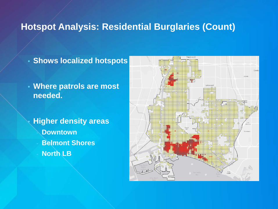
Hotspot Analysis: Residential Burglaries (Count)

• Shows localized hotspots

• Where patrols are most needed.

• Higher density areas- Downtown- Belmont Shores- North LB

Directional Distribution of Hotspot Analysis (Residential Burglary)

• Directional Distribution tool.

• Visualize changing spatial patterns.

• Ran hotspots for each year 2010 to 2014

• 1 Standard Deviation (68%) of weighted values (Gi_Bin)

• Very consistent pattern- Except 2011

Directional Distribution of Hotspot Analysis (Street Assault/Battery and Street Robbery)

• Assault/Battery (left)– shifting focus on downtown• Robbery (right)– increasing focus on downtown.

Hotspot Analysis by Police Patrol District

• Within each patrol district, where should officers spend more time?

• Hotspot analysis compares mean of search window to mean of study area.

• Different mean in each patrol district.

Hotspot Analysis by Police Patrol District

• Robbery (left) and Burglary (right)• Narrows hotspots around downtown• Expands hotspots around east LB

Hotspot Analysis: Rates

• Based on US Census Block Groups

• American Community Survey data (5 yr.)- Comes at block group level

• Most rates based on population.

• Burglary rates based on housing units.

• Wanted “neighborhood” scale. - 3000 foot distance threshold- Based on larger block groups in east

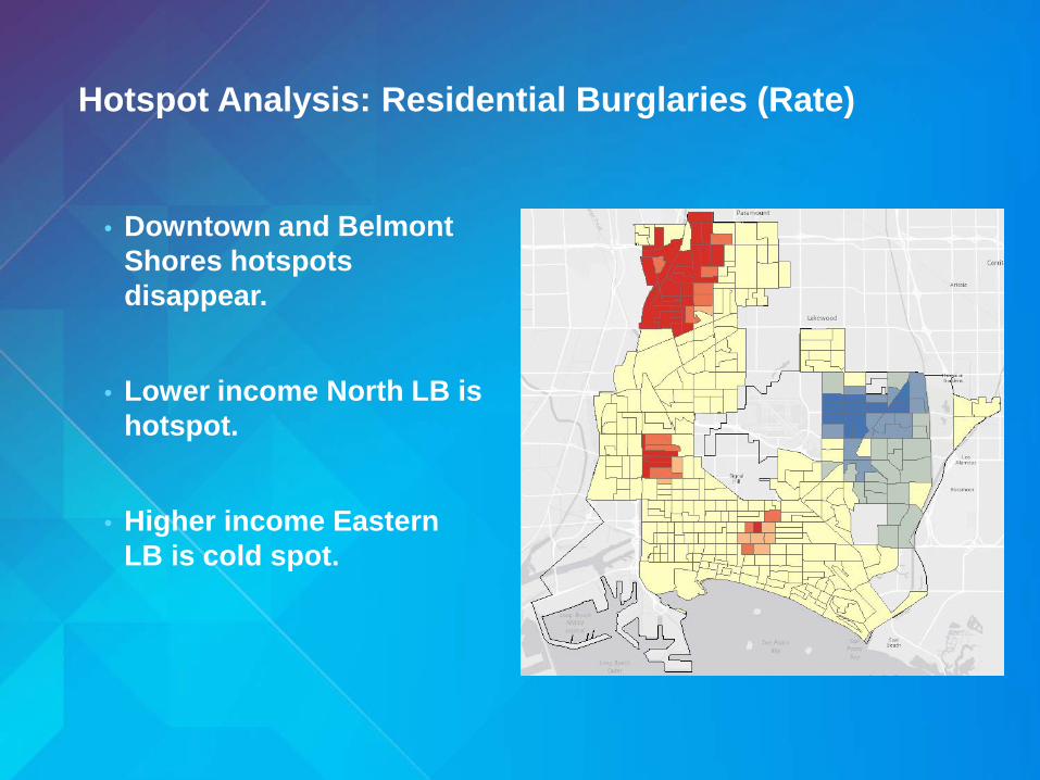
Hotspot Analysis: Residential Burglaries (Rate)

• Downtown and Belmont Shores hotspots disappear.

• Lower income North LB is hotspot.

• Higher income Eastern LB is cold spot.

Residential Burglaries: North LB Hot Spot

Residential Burglaries: East LB Cold Spot

Hotspot Analysis: Assault/Battery and Robbery(Rate)

• Assault/Battery (left), Robbery (right)• Clearly around downtown.

Assault/Battery and Robbery: Downtown

• Commercial and pedestrian activity.

• Pine St.• Anaheim St. and

PCH.

Regression Analysis

• Test Social Disorganization Theory

- Shaw and Mckay (1940s-60s)

- Crime is place specific.

- Lack of social controls to guide personal behavior due to neighborhood instability.

- Measured arrest rate vs. poverty, ethnic heterogeneity, and population turnover.

-

Regression Analysis

• My dependent variable- Arrest/Citation Rate

• My independent variables (from ACS 5 yr. Block Groups)- Percent less than high school- Percent unemployment- Diversity Index- Percent poverty- Year of residence- Percent households with over 1 person per room- Percent vacant housing units- Percent renters- Percent speaking English only- Per capita income- Percent of single mothers- Distance from crime hotspots- Percent using public transit

Regression Analysis

• Exploratory Regression tool.- Great Esri documentation.

- Interpreting Exploratory Regression Results- What they don't tell you about regression analysis

• Could not get passing models.- Failing Jarque-Bera test. - Looked at histograms. - Log transformed variables if they were skewed (not normally

distributed)- Removed 11% of block groups with zero people arrested.

Regression Analysis

• Exploratory Regression- After working with data– multiple passing models

- Selected model based on- Simplicity (fewer variables are better)- Match with theory (didn’t select distance-to-crime-hotspot)- R2 (higher) and AICc (lower)

Regression Analysis

• Ordinary Least Squares Regression tool

- Dependent variable - Log Arrest/Citation

- Independent variables (with coefficients)- Percent Renter (+0.681307) - Percent English Only (-0.714586)- Log Percent Poverty (+0.152645)- Log Per Capita Income (-0.370633)

- Adjusted R2 of 0.55

Regression Analysis: Interpretation

• Arrest/Citation rates increase as block groups have - Higher rates of poverty- Larger percentage of rental housing- Lower rates of English speaking- Lower per capita incomes

• Supports Social Disorganization theory.• Shaw and Mckay

• Poverty

• Ethnic heterogeneity

• Population turnover.

Regression Analysis: Interpretation

• Adjusted R2 of 0.55

• Still missing about 50% of explanatory power.

• Missing variables that can influence arrest rates?- Gang membership rate- Racial profiling- Police deployment patterns- Other?

Regression Analysis: Policy Implications

• Reduce Social Disorganization- Population turnover (stability with knowing neighbors).

- First time homeowner assistance.

- Ethnic heterogeneity (lack of integration/communication with neighbors/authorities)

- Expand ESL for adults/children- More multilingual public services.

- Economic condition- Upgrade skills/job training- Employment programs

Distance: Arrestee to Crime and Victim to Crime

• Test Crime Pattern Theory - Crimes occur in activity space of individuals.- Overlap of perpetrators and victims in spatial context.

- Within neighborhoods- Commercial areas- Entertainment areas- Downtown- Etc.

- Criminals work in places they are familiar with.

Distance: Arrestee to Crime and Victim to Crime

- Add XY fields to geocoded points for peoples’ addresses.

- Add XY fields to geocoded points for crimes.

- JOIN people and crime layers based on a crime ID field.

- XY to Line tool- Get length field

Distance: Arrestee to Crime

• Assault/Battery: - 33% same address- 43% within 500’

• Robbery - 23% within 1500’- 37% within 3000’- 52% within 1 mile

Distance: Arrestee to Crime

• Burglary- 35% within 3000 feet- 47% within 1 mile

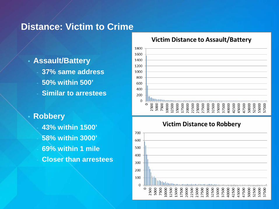
Distance: Victim to Crime

• Assault/Battery- 37% same address- 50% within 500’- Similar to arrestees

• Robbery- 43% within 1500’- 58% within 3000’- 69% within 1 mile- Closer than arrestees

Distance: Arrestee to Crime and Victim to Crime

• Classic distance decay patterns- People move more within places close to home.

• Supports Crime Patterns Theory- Overlapping activity spaces in local areas

- Neighborhood streets- Neighborhood shopping areas- Neighborhood entertainment

• Policy Implications- Crime prevention education- More community watch (less social disorganization)

:Conclusion

• Take care with geocoding.• Think about your scale of analysis with hotspots.• Use theory to guide regression analysis.• Exploratory Regression tool to find valid models.

- Careful with non-normal distributions!

• Run OLS Regression with final model.• Use XY to Line tool to see spatial relationships between

arrestees/victims/crime location

• Special thanks to - Rethinking Greater Long Beach

•