Embed Size (px)
Citation preview

Calhoun: The NPS Institutional Archive
DSpace Repository
Reports and Technical Reports All Technical Reports Collection
1988-05
A program to compute magnetic anomaly
detection probabilities
Forrest, R. N.
Monterey, California. Naval Postgraduate School
http://hdl.handle.net/10945/30103
Downloaded from NPS Archive: Calhoun
^/Z3
NPS71-88-001
NAVAL POSTGRADUATE SCHOOL
Monterey, California
A PROGRAM TO COMPUTE MAGNETIC ANOMALYDETECTION PROBABILITIES
R.N. FORREST
May 1988
Approved for Public Release; Distribution UnlimitedPrepared for:
Naval Postgraduate School
Monterey, CA 93943-5000
FedDocsD 208.14/2NPS-71-88-001

3".
NAVAL POSTGRADUATE SCHOOLMonterey, California
Rear Admiral Re C« Austin k. To MarshallSuperintendent Acting Provost
Reproduction of all or part of this report is authorized
.
This report was prepared byjI
UNCLASSIFIEDSECURITY CLASSIFICATION OF THIS PAGE
DUDLEY KNOtt LIBRARYREPORT DOCUMENTATION PAGE NAVAL POSTGRADUATE SCHOOL
6/lOMTEREV 0* 03043 51 1la REPORT SECURITY CLASSIFICATION
UNCLASSIFIEDlb RESTRICTIVE MARKING
2a SECURITY CLASSIFICATION AUTHORITY
2b. DECLASSIFICATION /DOWNGRADING SCHEDULE
3 DISTRIBUTION/AVAILABILITY OF REPORT
Approved for public release; distribution is
unl imited.
4. PERFORMING ORGANIZATION REPORT NUMBER(S)
NPS71-88-001
5 MONITORING ORGANIZATION REPORT NUMBER(S)
6a. NAME OF PERFORMING ORGANIZATION
Naval Postgraduate School
6b OFFICE SYMBOL(If applicable)
Code 71
7a NAME OF MONITORING ORGANIZATION
6c. ADDRESS (City, State, and ZIP Code)
Monterey, CA 93943-5000
7b. ADDRESS (City, State, and ZIP Code)
8a. NAME OF FUND'NG / SPONSORINGORGANIZATION
Naval Postgraduate School
8b OFFICE SYMBOL(If applicable)
9 PROCUREMENT INSTRUMENT IDENTIFICATION NUMBER
DIRECT FUNDING8c. ADDRESS (City, State, and ZIP Code)
Monterey, CA 93943-5000
10 SOURCE OF FUNDING NUMBERS
PROGRAMELEMENT NO
PROJECTNO
TASKNO
WORK UNITACCESSION NO
11. TITLE (Include Security Classification)
A PROGRAM TO COMPUTE MAGNETIC ANOMALY DETECTION PROBABILITIES
12. PERSONAL AUTHOR(S)
Forrest, R.N.
13a. TYPE OF REPORTTechnical
13b TIME COVEREDFROM TO
14 DATE OF REPORT (Year, Month, Day)OF REPORT (
1988 May15 P COUNT
16. SUPPLEMENTARY NOTATION
17 COSATI CODES 18 SUBJECT TERMS (Continue on reverse if necessary and identify by block number)
Magnetic Anomaly Detection, MAD, Lateral Range Function,
Detection Models
FIELD GROUP SUB-GROUP
19 ABSTRACT (Continue on reverse if necessary and identify by block number)
The report contains user instructions, a listing and documentation for a
microcomputer BASIC program that can be used to compute an estimate of the probability
that a magnetic anomaly detection (MAD) system such as the AN/ASQ-81 will detect a
submarine during an encounter.
20 DISTRIBUTION /AVAILABILITY OF ABSTRACT
%] UNCLASSIFIED/UNLIMITED D SAME AS RPT Q DT1C USERS
21 A8STRACT SECURITY CLASSIFICATION
Unclassi fied22a. NAME OF RESPONSIBLE INDIVIDUAL
Professor R.N. Forrest22b TELEPHONE (Include Area Code)
(408)646-265322c OFFICE SYMBOL
Code 55Fo
DDFORM 1473. 84 mar J3 APR edition may be used until exhausted
All other editions are obsoleteSECURITY CLASSIFICATION OF THIS PAGE
tt U.S. Government Printing Office. 1986—606-243


The program in this report is presented without representation orwarranty of any kind.


Table of Contents
I
.
Introduction 1
II. Program User Instructions 3
III. Encounter Model Limitations 6
IV. Parameter Values 9
Appendix 1. The Detection Statistics 12
Appendix 2. Program Probability Calculations 18
Appendix 3 . The Magnetic Signal 2
Appendix 4. The Anderson Formulation 24
Appendix 5. The Encounter Eguations of Motion 3
Appendix 6. The Submarine Magnetic Dipole 3 3
Appendix 7. The Earth Magnetic Field and Dip Angle-
•
3 6
Appendix 8. An Alternative Encounter Model 41
Appendix 9. An Example of the Program Output 4 3
Appendix 10. A Program Listing 49
References 59

I . Introduction
This report contains user instructions, a listing and
documentation for a microcomputer BASIC program that can be used
to compute an estimate of the probability that a magnetic
anomaly detection (MAD) system such as the AN/ASQ-81 will detect
a submarine during an encounter.
The program generates detection probabilities based on two
encounter models. In the first encounter model, the detection
system uses a crosscorrelation detector. In the second
encounter model, the detection system uses a sguare law detector.
Relative to operationally realizable values, probabilities based
on the first model represent upper bounds and those based on the
second model represent lower bounds. For both encounter models,
a magnetometer signal is proportional to the magnitude of the
projection of an anomaly field on the earth field, a submarine
anomaly field is a dipole field and the earth field and the noise
do not change with changes in the position of the magnetometer.
Also, for both encounter models, an encounter is a straight line
encounter with constant vertical separation.
The encounter models can be interpreted as models of a
magnetic anomaly detection system on an aircraft that is moving
with constant course, speed and altitude in an encounter with a
submarine moving with constant course, speed and depth. Or, they
can be interpreted as models of a stationary magnetic anomaly
detection system in an encounter with a submarine moving with
constant course, speed and depth.
The program parameters include encounter latitude and
longitude, submarine induced magnetic moments, submarine
permanent magnetic moments, submarine course, speed and altitude,
magnetometer course, speed and depth, encounter lateral range
(the horizontal range at the closest point of approach in a
straight line encounter) and false alarm rate. (In the program,
a false alarm is the event that the detection system classifies
noise as a dipole signal.)
II. Program User Instructions
As listed in Appendix 10, the program can be run under a
BASIC language that is compatible with IBM PC BASIC. If the
listing is used to enter the program through the keyboard, then
the program should be saved with the name MAD.BAS or the value of
N$ on line 20 should be changed to the file name under which it
is saved.
The program contains user instructions in the form of query
and parameter limitation messages. As an example of the former,
after starting the program under BASIC, the following message
should appear:
Magnetic Anomaly Detection (MAD) Lateral Range Function
generate or print a program data file (g/p)
?
By entering p, data can be printed from a program data file
that was generated by the program. By entering g, a program
data file can be generated for a set of user specified
conditions. With either response, a sequence of additional
queries is displayed. These queries require either an indicated
response or a parameter value as the input . If the initial
response is g, the sequence includes queries whose responses
determine whether or not an auxiliary data file will be generated
that can be used for future input of magnetic, processing or
kinematic data. In particular, the first query in the sequence
gives the option of using a combined magnetic, processing and
kinematic data file. If the response indicates that it should
3
be used and the file is available, the parameter values that
remain to be entered in order to generate a program data file are
the following: the false alarm rate, the magnetic noise, the
maximum encounter lateral range and the lateral range step. The
combined file should be used only if the effect of varying just
one or more of these parameters is desired. If the response
indicates that the file will not be used, queries concerning
magnetic, kinematic and processing parameter values are
displayed.
After all of the program parameter values have been
entered, a query is displayed giving the option of generating the
combined file. Then a query giving the option of generating a
program data file, a query giving the option of printing the
encounter parameter values and a query giving the option of
printing lateral range function values are displayed. The
lateral range function values are the encounter detection
probabilities indexed by lateral range. The parameters maximum
lateral range and lateral range step determine the index lateral
ranges of the encounters for which probabilities of detection are
computed.
The program generates magnetic signal values that correspond
to points in time during an encounter. Following the lateral
range function query, a query is displayed that gives the option
of printing the magnetic signal values for an encounter. If the
option is exercised, the option is repeated. When the option is
not exercised, a query is displayed that gives the option of

generating or printing a new program data file. If this option
is not exercised, the program ends.
Some suggested guides for determining parameter values can
be found in Section IV of this report.
III. Encounter Model Limitations
In the two encounter models, noise is determined by a
gaussian process. This may be a limitation in describing a
stationary magnetometer. In this case, the noise must account
for geomagnetic, instrument and magnetohydrodynamic noise. And
it may be a significant limitation if the magnetometer is
moving. In this case, in addition to the above sources, the
noise must account for maneuver noise and geologic noise.
The signal is that of a magnetic dipole that moves relative
to the magnetometer. Describing a ship magnetic anomaly as a
dipole anomaly should not be a significant limitation for
encounter slant range at the closest point of approach (CPA) that
is greater than one hull length. The detection decision is
based on samples from a single time interval (window) that is
centered on the CPA. The length of the sampling interval and the
sampling rate are parameter values that are inputs to the
program. In terms of signal-to-noise ratio, there is an optimum
sampling interval length (integration time) and sample rate.
Although dipole signal energy is not symmetrically distributed
about the CPA time, for a given sampling interval, the difference
between the signal energy for the optimum interval location and
the CPA centered location should not be significant in most
cases.
The encounter model magnetometer noise samples are values of
independent identically distributed random variables. The
standard deviation of these random variables is referred to as
the magnetic noise and the variance is the noise in the sense of
the signal-to-noise ratio. The magnetic noise of the encounter
models is determined by a gaussian random process. The degree of
correspondence between this process and operational noise
depends on the nature of the dominant operational noise sources
and on the magnetometer input filtering (noise whitening)
.
In the encounter models, the intervals are adjacent but not
overlapping and a detection statistic corresponds to each sample
interval and its value is determined by the sample values. If
the value of the detection statistic for an interval equals or
exceeds a threshold value, a detection is indicated. The
threshold value is determined by the false alarm probability
which in turn is determined by the false alarm rate and the
sampling interval length.
A detector that used a moving sample interval that was
generated by replacing the oldest sample by the newest one would
correspond more closely to the detector in an operational
detection system. In a model of the detector, since the sample
windows overlap, the detection statistics would represent a
sequence of random variables that were correlated over an
interval equal to the width of the sample interval. Because of
this dependence, it seems unlikely that the results that would be
obtained with an encounter model based on an overlapping interval
detector would differ significantly from those obtained with an
encounter model based on a nonoverlapping interval detector.
For encounter lengths of the order of a few nautical miles
or less, the straight line encounter condition should not be a
significant limitation. In particular, this should be the case
for a fixed magnetometer since, for a submarine (or surface ship)
target, vertical separation and course changes should be less
likely to occur.
Other models are available that can be used as the basis for
computing an estimate of the probability that a magnetic anomaly
detection system will detect a submarine during an encounter.
For example, one that is described in Appendix 8 can be used to
determine the slant ranges of straight line encounters for which
the detection probability is equal to a specified value. The
parameter values that are required to do this are an average
submarine dipole moment, a detection system capability factor and
a noise factor. Values for these parameters can be determined
from operational data. However, the values are specific to
averages over a particular set of encounter conditions. An
advantage of the two encounter models relative to this model is
their adaptability to different magnetic, processing and
kinematic conditions.
IV. Parameter Values
The magnetic parameter value queries are generally
explanatory with regard to the value that should be entered.
This is also true of the kinematic parameter value queries.
However, there is some ambiguity with respect the processing
parameter value queries and the noise parameter value query. To
reduce this ambiguity, a brief discussion of the common
characteristics of the two encounter model processing parameters
and the noise parameter is given below. This is followed by
some guidelines for choosing these parameter values.
In both encounter models, a decision is made at the end of
each sampling interval. The decision is either noise energy was
present during the interval or noise energy plus signal energy
was present during the interval. The sample intervals are
adjacent, equal width, nonoverlapping time intervals. The number
of samples that are input in a sample interval is determined by
the sampling rate and the interval length.
The program default choice for the sampling rate is 2MAXF
where MAXF is a parameter that is labeled the maximum magnetic
signal frequency. This sample rate is the Nyquist rate for an
ideal low pass filter. However, the signal in a sample interval
that is computed by the program represents an unfiltered dipole
signal. This is a reasonable approximation if the signal energy
that is associated with signal components greater than MAXF is
relatively small. As discussed below, the noise energy in a
sample interval should be considered to be proportional to MAXF
in order to be consistent with the encounter models. Ideally, a
default choice for MAXF would make the ratio of the signal energy
to the noise energy a maximum for the sampling interval of an
encounter. The program default choice for MAXF is 2• MAXVM/MINRO
where MAXVM is a user estimated maximum encounter relative speed
converted from knots to meters per second and MINRO is a user
estimated maximum slant range at CPA in meters in terms of a just
detectable target. (A precise definition of a just detectable
target can be made in terms of a specified detection probability,
false alarm probability and target dipole moment.) The default
choice for MAXF is consistent with the observation in Reference 1
that if an optimum value for MAXF is determined for a minimum
dipole moment target, then no significant increase in MAXF is
required in order to maintain a required detection probability if
the encounter lateral range is decreased even though the signal
energy spectrum is shifted to higher frequencies.
Because of the detection statistics and the gaussian noise
model, if there were no penalty for decision delay, a sample
interval length for a signal should be chosen equal to the signal
duration, since this would make the detection probability for an
encounter a maximum. In the program, a default choice for the
sample interval length (integration time) is 2• MAXRO/MINVM where
MINVM is a user estimated maximum encounter relative speed
converted from knots to meters per second and MAXRO is a user
estimated maximum slant range at CPA in meters for a detectable
encounter (in terms of a specific detection probability and false
10
alarm probability) with a user specified maximum dipole moment
target. This choice might be considered a balance between
minimizing decision delay and maximizing detection probability.
In the encounter models, the sample intervals are located so that
the CPA time is at the center of a sample interval and this
sample interval is the only one that contains signal energy.
This characteristic is consistent with the default choice for the
sample interval. For a given sample interval length, although in
general the interval location is not the optimum one in terms of
signal energy, it should be approximately so in most cases.
The program noise parameter is SIG. It represents the
standard deviation a associated with the magnetic noise process
of the two encounter models. In terms of the ideal low pass
filter implied by the encounter models, its sguare should be
equal to MAXF-(SIGO) 2 where SIGO is the magnetic noise process
constant power spectral density. The program does not enforce
this relation. Therefore, in using the program, the implied
relation between the two input parameters: magnetic noise and
maximum magnetic signal frequency should be kept in mind. If an
average value of the peak-to-peak magnetic noise for an encounter
can be estimated, for example from a magnetometer trace, then the
value for SIG should be chosen so that the estimate is 4 to 6
times this value.
11
Appendix 1. The Detection Statistics
In this appendix, Y\i Y2' '*'' Ym are sequential values
(voltages) representing the sample values in a sample interval.
They are the input to a magnetometer's detector. With these m
sample values, the detector computes the value of a detection
statistic. This value is represented by x and the detection
decision corresponding to the sample interval is determined by
the decision rule: If x > x*, then the input during the sample
interval was noise plus signal, otherwise, the input was noise.
For both encounter models, the detection probability and the
false alarm probability are decreasing functions of x* and the
relation is one-to-one in both cases. In the program, the false
alarm probability pf is used to determine a unique value of
the threshold x*. This value is then used to determine a unique
value of the detection probability p<~j.
In the program, pf is found using the relation pf = R-St
where R is the false alarm rate in false alarms per second
and St is the sample interval length in seconds. This relation
is based on the following argument: With no signal energy in a
sample interval, y^_ = n^, Y2 = n2 ' ' ' *' Ym = nm where n^, n 2 ,
•••, nm are noise values (voltages) input to a magnetometer's
detector. The n-j_ are values of independent normal (gaussian)
random variables, each with mean zero and standard deviation a.
Because of this, in the encounter models, values of x for
different sample intervals are the values of independent random
variables that determine two outcomes: x > x* or x < x*.
12
Therefore, in terms of these outcomes, an encounter is a sequence
of independent Bernoulli trials. If there is no signal present,
since the noise is determined by a stationary process, pf is the
same for each sample interval and, in terms of these outcomes,
the sequence is a series of repeated independent Bernoulli trials
and therefore the expected number of trials between false alarms
is 1/Pf- Since the time between trials is St, the expected
number of seconds between false alarm is St/pf or the expected
number of false alarms per second R is equal to pf/St.
The determination of x* depends on the encounter model
statistic. For both encounter models, when there is a signal,
Yl = n x + s lt y 2 = n 2 + y 2 ,• •
• , ym = nm + sm where s 1# s 2 ,
•••, sm are signal values (voltages) input to a magnetometer's
detector. The models imply that the signal values s^ = K- (Hs )
^
where K is a constant whose value is determined by the
characteristics of the encounter magnetometer and where the
(Hs ) j_ are dipole magnetic signal intensities. The models also
imply that the noise values n-j_ are determined by a gaussian
stochastic processes characterized by a standard deviation a
and that n-j_ = K- (HN ) j_+ n-j_ where the (HN ) j_
are magnetic noise
intensities and the n-j_ are magnetometer instrument noise values
(voltages). In the program, the magnitude of K is 1. Since,
for both models, p^ depends only on the ratio of signal energy
to noise energy for a sample interval, this is a satisfactory
choice for the program if instrument noise is assumed to be
determined by a process independent of the magnetic noise process
13
and to be expressed in terms of an equivalent magnetic noise
(H)i = (1/K) -n[.
For both encounter models, the signal (the average signal
2
power) S = (1/m) S Sj_ and the noise (the expected value of the
2
average noise power) N = a so that the signal-to-noise ratio
is (1/m) -2 s-^/a where the sum index l = 1, 2, • • •, m.
The Crosscorrelation Detector Statistic: The statistic for the
first encounter model is a crosscorrelation detector statistic
that is defined by the sum
x = S Yi'S±
where the summation index i = 1, 2, , m and the sum is over
the values corresponding to a sample interval. For the first
encounter model, the characteristics of both the noise and the
signal are required in order to determine encounter detection
probabilities. In particular, the signal values for an encounter
are in the memory of the detector prior to the encounter. For
the encounter conditions and a specified false alarm
probability, the statistic is optimum in the sense that the
encounter detection probability for this statistic is at least
equal to that for any other statistic. Because of these
considerations, encounter probabilities based on the
crosscorrelation statistic can be considered to represent upper
bounds on detection performance against dipole targets for
magnetometers of the type described by the models.
For a sample interval without signal energy, x is the value
of a normal random variable with a mean (j,x = and a variance
14
&X = ° ' s s i where a is the standard deviation associated with
the noise process and the sum index 1=1, 2, • •
• , m and the
sum is over the values corresponding to the sample interval.
This implies that
p f = 1 - P(x*/ax )
where P(z) is the standard normal cumulative distribution
function. This relation is the basis for determining the
threshold value x*.
For the sample interval with signal energy, x is the value
2
of a normal random variable with a mean p.^ = 2 s-j_ where the sum
index i = 1, 2, • •• , m and the sum is over the values
corresponding to the sample interval. This implies that
pd = 1 - P(v* - d*)
where v* = x*/ax and d = S s^/a 2 = (1/m) -S/N. This relation
is the basis for determining encounter detection probabilities
for the first encounter model. The relation implies that for a
specified false alarm probability pf the detection probability
p<3 is an increasing function of the signal to-noise ratio S/N.
The Square Law Detector Statistic: The statistic for the second
encounter model is a square law (energy) detector statistic that
is defined by the sum
x = 2 y[
where the sum index i = 1, 2, • •
• , m and the sum is over the
values corresponding to the sample interval. For the second
encounter model, only the characteristics of the noise are
required to determine encounter detection probabilities.
15
For a sample interval without signal energy, x/a 2 is the
value of a chi-square random variable with m degrees of
freedom. This implies that
p f = 1 - P(x*/°2
|m)
where P(x /a |m) is the chi-square cumulative distribution
function for a chi-square random variable with m degrees of
freedom and where a is the standard deviation associated with
the noise process. This relation is the basis for determining
the threshold value x*
.
,2
For the sample interval with signal energy, x/a is the
value of a noncentral chi-square random variable with m
2 2
degrees of freedom and noncentral parameter S s-j_/a where the
sum index i = 1, 2, • •• , m and the sum is over the values
corresponding to the sample interval. This implies that
pd = 1 - F(x*/o2
\m, S s^/a2
)
JL 2 . 2 2,where P(x /a |m, 2 s-j/a ) is the noncentral chi-square
cumulative distribution function for a noncentral chi-square
random variable with m degrees of freedom and noncentral2 2
parameter 2 s-j_/a = (1/m) -S/N. This relation is the basis for
determining encounter detection probabilities for the second
encounter model. The relation implies that for a specified false
alarm probability pf, the detection probability pd is an
increasing function of the signal-to-noise ratio S/N. This is
made more evident by the following relation:
P(x*/</|m, 2 Si/a') = 2 { (a^/j!) -exp(-a) -P[x*/cr2
|
(m + 2- j) ]}
where a = (1/2) -2 s-^/a = (m/2) • (S/N), the sum index i = 1, 2,
16

• •• , m and the sum index j = 0, 1,2, •••
. (Note, p^ > pf
,
as expected, since P(x*/a 2|m) ^ P[x*/a 2 |(m + 2-j)] for j = 0,
1, 2, • .)
17
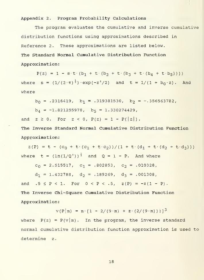
Appendix 2 . Program Probability Calculations
The program evaluates the cumulative and inverse cumulative
distribution functions using approximations described in
Reference 2. These approximations are listed below.
The Standard Normal Cumulative Distribution Function
Approximation :
P(z) = 1 - s-t-(b-L + t- (b 2 + t- (b 3 + t- (b 4 + t-b 5 ))))
where s = (1/ (2 • tt) * ) • exp (-z 2/2) and t = 1/(1 + b -z). And
where
b = .2316419, b1 = .319381530, b2 = -.356563782,
b 4 = -1.821255978, b 5 = 1.330274429,
and z > 0. For z < 0, P(z) = 1 - P(|z|).
The Inverse Standard Normal Cumulative Distribution Function
Approximation :
z(P) - t - (c + t-( Cl + t-c 2 ))/(l + t-(dx + t-(d 2 + t-d 3 )))
where t = (ln(l/Q 2
))2 and Q = 1 - P. And where
c = 2.515517, c ± = .802853, c2 = .010328,
d ± = 1.432788, d 2= .189269, d 3
= .001308,
and .5 < P < 1. For < P < .5, z(P) = -z(l - P)
.
The Inverse Chi-Square Cumulative Distribution Function
Approximation :
v(p|m) = m- [1 - 2/(9-m) + z• (2/ (9
• m) ) I
]
3
where P(z) = P(v|m). In the program, the inverse standard
normal cumulative distribution function approximation is used to
determine z
.
18

The Noncentral Chi-Square Cumulative Distribution Function
Approximation :
P(w|m,2 s-j/a ) = P(z)
where z = [2-w/(l + b) ] I - [2-a/(l + b) - l]i with2 2 2 2 2 2
a = m + Z Sj[/a , b = (S Sj_/a )/(m + s s-j_/a ) and the sum index
i = 1, 2, , m. In the program, the standard normal
cumulative distribution function approximation is used to
determine P(z)
.
19
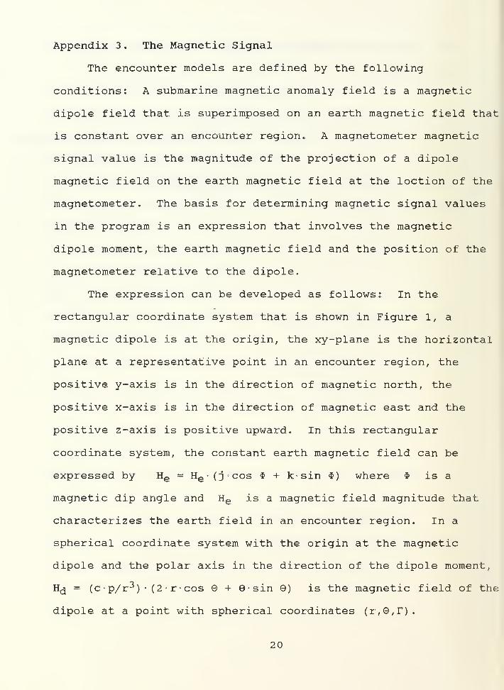
Appendix 3 . The Magnetic Signal
The encounter models are defined by the following
conditions: A submarine magnetic anomaly field is a magnetic
dipole field that is superimposed on an earth magnetic field that
is constant over an encounter region. A magnetometer magnetic
signal value is the magnitude of the projection of a dipole
magnetic field on the earth magnetic field at the loction of the
magnetometer. The basis for determining magnetic signal values
in the program is an expression that involves the magnetic
dipole moment, the earth magnetic field and the position of the
magnetometer relative to the dipole.
The expression can be developed as follows: In the
rectangular coordinate system that is shown in Figure 1, a
magnetic dipole is at the origin, the xy-plane is the horizontal
plane at a representative point in an encounter region, the
positive y-axis is in the direction of magnetic north, the
positive x-axis is in the direction of magnetic east and the
positive z-axis is positive upward. In this rectangular
coordinate system, the constant earth magnetic field can be
expressed by He = He - (j-cos $ + k-sin §) where $ is a
magnetic dip angle and He is a magnetic field magnitude that
characterizes the earth field in an encounter region. In a
spherical coordinate system with the origin at the magnetic
dipole and the polar axis in the direction of the dipole moment,
H3 = (c-p/r 3)
•(2-r-cos 9 + 8- sin 0) is the magnetic field of the
dipole at a point with spherical coordinates (r,9,r).
20
Hd/Hd
dipole
MagneticNorth
MagneticEast
Polar Axis
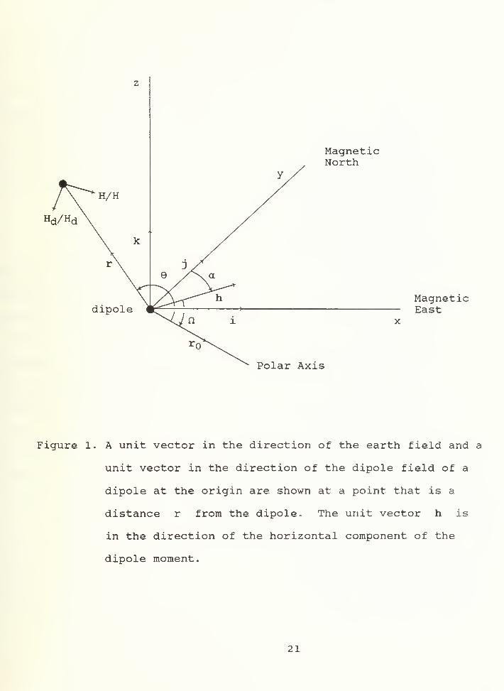
Figure 1. A unit vector in the direction of the earth field and a
unit vector in the direction of the dipole field of a
dipole at the origin are shown at a point that is a
distance r from the dipole. The unit vector h is
in the direction of the horizontal component of the
dipole moment.
21
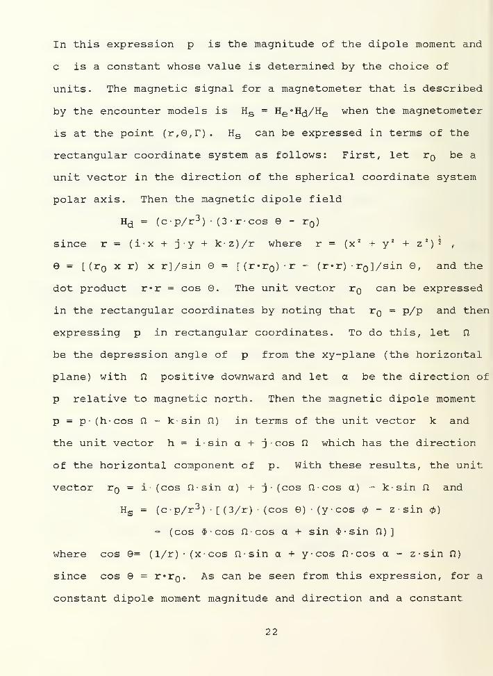
In this expression p is the magnitude of the dipole moment and
c is a constant whose value is determined by the choice of
units. The magnetic signal for a magnetometer that is described
by the encounter models is Hs = He o H^/He when the magnetometer
is at the point (r,9,r). Hs can be expressed in terms of the
rectangular coordinate system as follows: First, let r be a
unit vector in the direction of the spherical coordinate system
polar axis. Then the magnetic dipole field
Hd = (c-p/r 3)
•
(3-rcos e - r )
isince r = (ix + jy + k-z)/r where r = (x + y + z )
2,
9 =[ (r x r) x r]/sin 9 = [(r-r )-r - (r»r) •
r
]/sin 9, and the
dot product r«r = cos 9. The unit vector Tq can be expressed
in the rectangular coordinates by noting that Tq = p/p and then
expressing p in rectangular coordinates. To do this, let n
be the depression angle of p from the xy-plane (the horizontal
plane) with n positive downward and let a be the direction of
p relative to magnetic north. Then the magnetic dipole moment
p = p (h-cos n - k-sin f2) in terms of the unit vector k and
the unit vector h = i-sin a + j • cos n which has the direction
of the horizontal component of p. With these results, the unit
vector Tq = i- (cos II- sin a) + j • (cos a- cos a) - k-sin f2 and
Hs = (c-p/r 3)
•
[ (3/r) • (cos 9) • (y • cos - z • sin <p)
- (cos $• cos n-cos a + sin $-sin n)
]
where cos 9= (l/r)-(xcos fi-sin a + y-cos n-cos a - z-sin n)
since cos 9 = r-rp. As can be seen from this expression, for a
constant dipole moment magnitude and direction and a constant
22

earth field magnitude and direction, the magnetic signal is only
a function of the rectangular coordinates of the location of the
magnetometer relative to the dipole. In the encounter models,
both of these conditions are satisfied. However, by allowing p,
n, a, Hs and $ to vary, the expression for Hs is applicable
to more general encounter models.
23
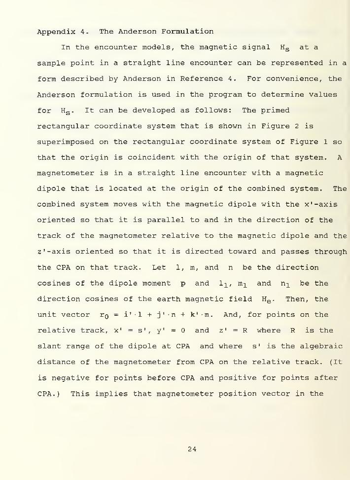
Appendix 4 . The Anderson Formulation
In the encounter models, the magnetic signal Hs at a
sample point in a straight line encounter can be represented in a
form described by Anderson in Reference 4. For convenience, the
Anderson formulation is used in the program to determine values
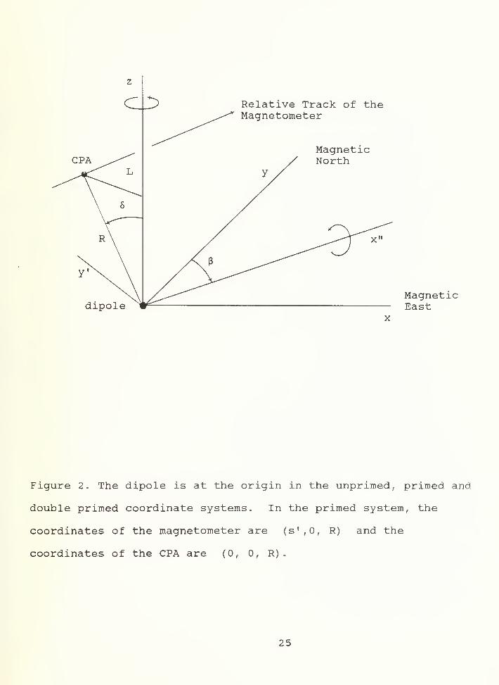
for Hs . It can be developed as follows: The primed
rectangular coordinate system that is shown in Figure 2 is
superimposed on the rectangular coordinate system of Figure 1 so
that the origin is coincident with the origin of that system. A
magnetometer is in a straight line encounter with a magnetic
dipole that is located at the origin of the combined system. The
combined system moves with the magnetic dipole with the x'-axis
oriented so that it is parallel to and in the direction of the
track of the magnetometer relative to the magnetic dipole and the
z ' -axis oriented so that it is directed toward and passes through
the CPA on that track. Let 1, m, and n be the direction
cosines of the dipole moment p and 1^, m^ and n-j_ be the
direction cosines of the earth magnetic field He . Then, the
unit vector r = i'-l + j'-n + k' -m. And, for points on the
relative track, x 1 = s', y
1 =0 and z' = R where R is the
slant range of the dipole at CPA and where s' is the algebraic
distance of the magnetometer from CPA on the relative track. (It
is negative for points before CPA and positive for points after
CPA. ) This implies that magnetometer position vector in the
24
Relative Track of theMagnetometer
MagneticNorth
MagneticEast
Figure 2. The dipole is at the origin in the unprimed, primed
double primed coordinate systems. In the primed system, the
coordinates of the magnetometer are (s',0, R) and the
coordinates of the CPA are (0, 0, R)
«
25
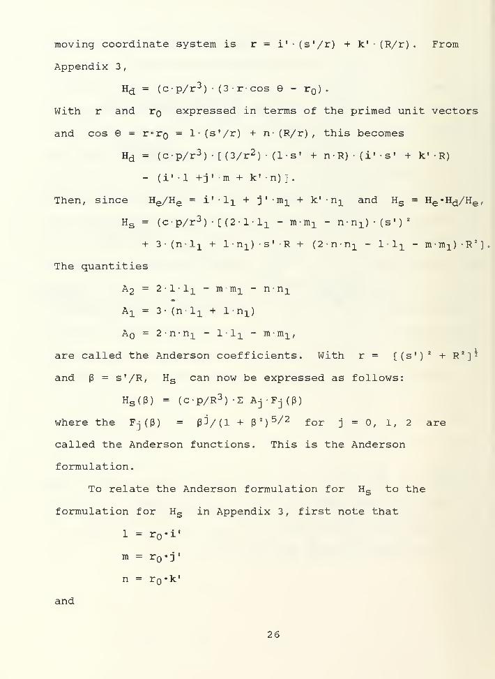
moving coordinate system is r = i'•(s'/ r ) + k'
•(R/r) . From
Appendix 3
,
Hd = (c-p/r 3)
•
(3• r-cos 9 - r )
.
With r and r expressed in terms of the primed unit vectors
and cos 8 = r-rg = 1- (s'/r ) + n " (R/r) t this becomes
Hd = (c-p/r 3) •[ (3/r 2
)•(1-s' + n-R)-(i'-s' + k» R)
- (i' 1 +j • -m + k' -n) ]
.
Then, since He/He = i'-l^ + j'-m^ + k' -n^ and Hs = He »Hd/He ,
Hs = (c-p/r 3) .[(2-1-1! - m-mx - n-n x )
•(s») 2
+ 3-(nl]_ + l-n^-s'R + (2-n-n x - l-li - m-m 1 )-R2
]
The quantities
A2 = 2-l-l]_ - m m^ - n-n!
A! = 3 (n- li + l-n^)
A = 2-n-n^ - llx ~ m-ni]_,
are called the Anderson coefficients. With r = [(s 1
)
2 + R 2
]5
and (3 = s'/R/ Hs can now be expressed as follows:
Hs ((3) = (c-p/R 3) -2 Aj-Fj(P)
where the Fj(P) = pV(l + (3*) 5/2 for j = 0, 1, 2 are
called the Anderson functions. This is the Anderson
formulation.
To relate the Anderson formulation for Hs to the
formulation for Hs in Appendix 3 , first note that
1 = r .i»
m = r -j"
n = r -k'
and
26
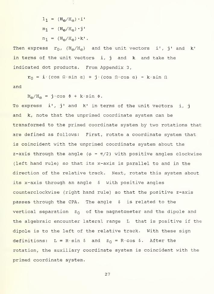
l x = (He/He )-i'
mx = (He/He ) -j'
n x = (He/He )-k«.
Then express r , (He/He ) and the unit vectors i' , j1 and k'
in terms of the unit vectors i, j and k and take the
indicated dot products. From Appendix 3,
r = i- (cos ft-sin a) + j•(cos n-cos a) - k-sin n
and
He/He = j • cos $ + k-sin $.
To express i 1
,j' and k' in terms of the unit vectors i, j
and k, note that the unprimed coordinate system can be
transformed to the primed coordinate system by two rotations that
are defined as follows: First, rotate a coordinate system that
is coincident with the unprimed coordinate system about the
z-axis through the angle (0 - tt/2) with positive angles clockwise
(left hand rule) so that its x-axis is parallel to and in the
direction of the relative track. Next, rotate this system about
its x-axis through an angle 5 with positive angles
counterclockwise (right hand rule) so that the positive z-axis
passes through the CPA. The angle S is related to the
vertical separation Zg of the magnetometer and the dipole and
the algebraic encounter lateral range L that is positive if the
dipole is to the left of the relative track. With these sign
definitions: L = R-sin 5 and Zg = R-cos 5. After the
rotation, the auxiliary coordinate system is coincident with the
primed coordinate system.
27
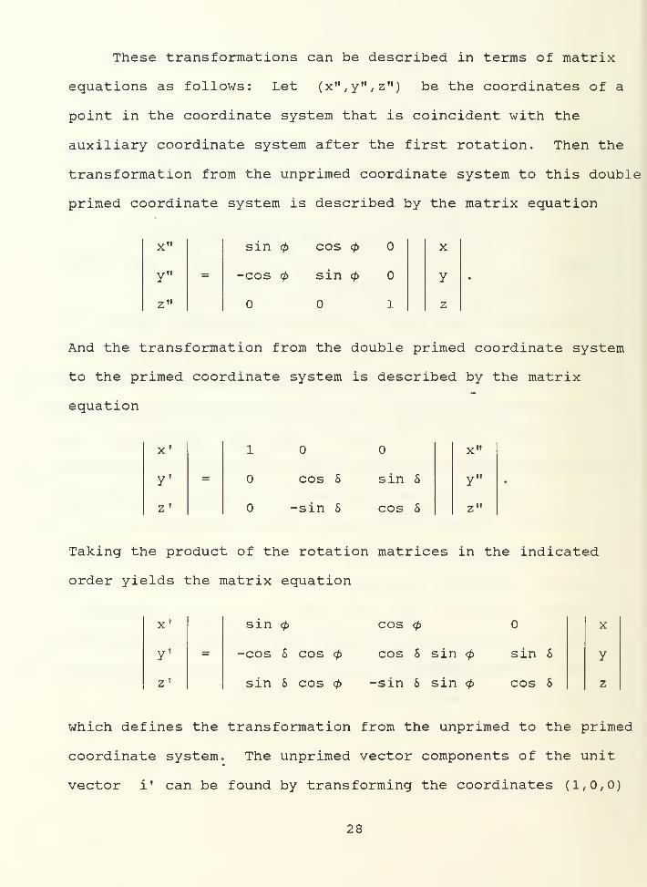
These transformations can be described in terms of matrix
equations as follows: Let (x" /y"
/ z") be the coordinates of a
point in the coordinate system that is coincident with the
auxiliary coordinate system after the first rotation. Then the
transformation from the unprimed coordinate system to this double
primed coordinate system is described by the matrix equation
X"
y" =
z"
sin cos
cos sin
1
x
y
z
And the transformation from the double primed coordinate system
to the primed coordinate system is described by the matrix
equation
X'
yz'
10cos S sin 5
-sin 5 cos 5
X"
y"
z"
Takinq the product of the rotation matrices in the indicated
order yields the matrix equation
x»
yz'
sin cos
•cos 6 cos cos 5 sin sin 5
sin S cos -sin 5 sin cos 5
x
y
z
which defines the transformation from the unprimed to the primed
coordinate system. The unprimed vector components of the unit
vector i 1 can be found by transforminq the coordinates (1,0,0)
28
in the primed system to their corresponding coordinates in the
unprimed system with the inverse of this matrix and then
repeating this process for (0,1,0) and (0,0,1) in order to find
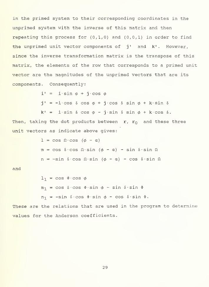
the unprimed unit vector components of j ' and k' . However,
since the inverse transformation matrix is the transpose of this
matrix, the elements of the row that corresponds to a primed unit
vector are the magnitudes of the unprimed vectors that are its
components. Consequently:
i" = i-sin + j cos
j" = -i-cos 5 cos + j • cos 5 sin + k-sin 5
k 1 = i-sin 5 cos - j • sin 5 sin + k-cos S.
Then, taking the dot products between r, r and these three
unit vectors as indicate above gives:
1 = cos n-cos (0 - a)
m = cos S cos n-sin (0 - a) - sin 6 -sin fi
n = -sin S • cos ft-sin (0 - a) - cos S-sin ft
and
1]_ = cos $ • cos
irt]_ = cos 5 • cos $sin - sin S-sin $
n^ = -sin 6• cos $sin - cos 5
• sin $.
These are the relations that are used in the program to determine
values for the Anderson coefficients.
29
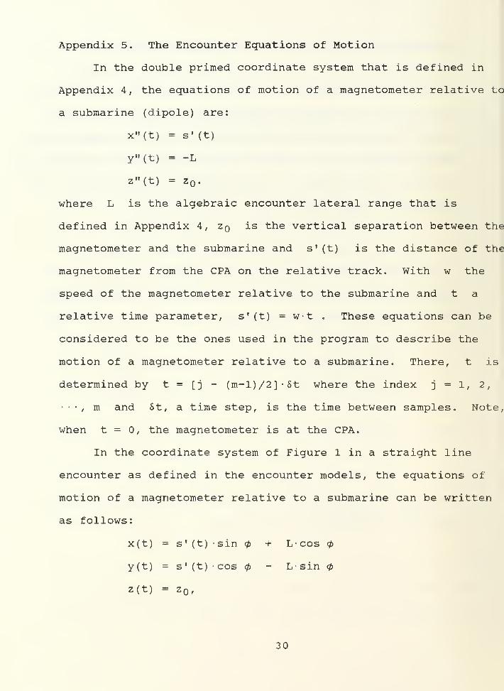
Appendix 5. The Encounter Equations of Motion
In the double primed coordinate system that is defined in
Appendix 4, the equations of motion of a magnetometer relative to
a submarine (dipole) are:
x"(t) = s» (t)
Y n (t) = -L
z"(t) = z .
where L is the algebraic encounter lateral range that is
defined in Appendix 4, Zq is the vertical separation between the
magnetometer and the submarine and s'(t) is the distance of the
magnetometer from the CPA on the relative track. With w the
speed of the magnetometer relative to the submarine and t a
relative time parameter, s'(t) = w-t . These equations can be
considered to be the ones used in the program to describe the
motion of a magnetometer relative to a submarine. There, t is
determined by t = [j - (m-l)/2]-St where the index j = 1, 2,
• • •, m and 6t, a time step, is the time between samples. Note,
when t = 0, the magnetometer is at the CPA.
In the coordinate system of Figure 1 in a straight line
encounter as defined in the encounter models, the equations of
motion of a magnetometer relative to a submarine can be written
as follows:
x(t) = s'(t)sin + L-cos
y(t) = s' (t) cos - L-sin <p
z(t) = z,
30
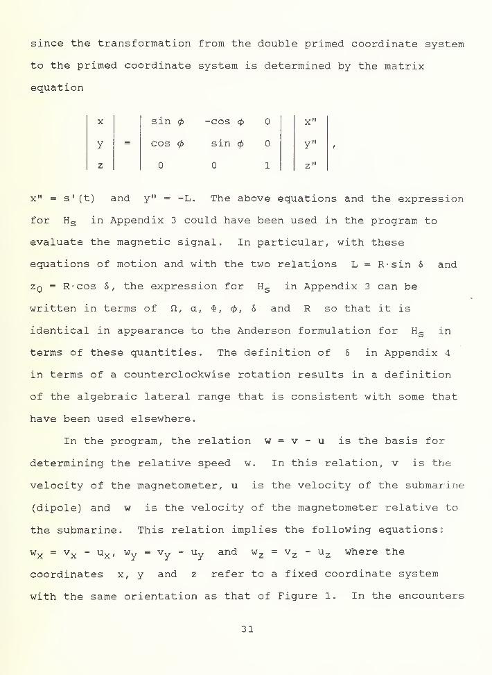
since the transformation from the double primed coordinate system
to the primed coordinate system is determined by the matrix
equation
x
Y
z
sin -cos
cos sin
1
X"
yii
Z"
x" = s'(t) and y" = -L. The above equations and the expression
for Hs in Appendix 3 could have been used in the program to
evaluate the magnetic signal. In particular, with these
equations of motion and with the two relations L = R-sin 5 and
Zq = R-cos 5, the expression for Hs in Appendix 3 can be
written in terms of f2, a, $, 0, 5 and R so that it is
identical in appearance to the Anderson formulation for Hs in
terms of these quantities. The definition of 5 in Appendix 4
in terms of a counterclockwise rotation results in a definition
of the algebraic lateral range that is consistent with some that
have been used elsewhere.
In the program, the relation w = v - u is the basis for
determining the relative speed w. In this relation, v is the
velocity of the magnetometer, u is the velocity of the submarine
(dipole) and w is the velocity of the magnetometer relative to
the submarine. This relation implies the following equations:
wx = vx - ux , Wy = Vy - Uy and w z = v 2- u z where the
coordinates x, y and z refer to a fixed coordinate system
with the same orientation as that of Figure 1. In the encounters
31
of the models, vx = v-sin a, Vy = v-cos a and v 2 = where a
is the magnetic course and v is speed of the magnetometer.
And, ux = u-sin (3 , Uy = u-cos 3 and u z = where 3 is the
magnetic course and u is the speed of the submarine. The
relative magnetic course and the relative speed of the
magnetometer are defined by wx = w-sin and wy = w-cos 0. In
the program, and w are determined with a rectangular to
ipolar conversion routine where w = ( wx + Wy) 2 and where is
determined by sin-1 (wx/w) and cos-1 (Wy/w)
.
32
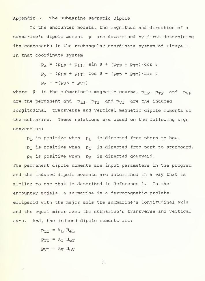
Appendix 6. The Submarine Magnetic Dipole
In the encounter models, the magnitude and direction of a
submarine's dipole moment p are determined by first determining
its components in the rectangular coordinate system of Figure 1.
In that coordinate system,
Px = (PLP + PLl) sin P + (PTP + PTl) -cos P
Py = (PLP + PLl)' cos P " (PTP + PTl)
'
sin P
Pz = "(PVP + Pvi)
where 3 is the submarine's magnetic course, Plp, p<i>p and pvp
are the permanent and PlI/ Pti anc^ Pvi are the induced
longitudinal, transverse and vertical magnetic dipole moments of
the submarine. These relations are based on the following sign
convention:
pL is positive when pL is directed from stern to bow.
pT is positive when pT is directed from port to starboard.
pv is positive when py is directed downward.
The permanent dipole moments are input parameters in the program
and the induced dipole moments are determined in a way that is
similar to one that is described in Reference 1. In the
encounter models, a submarine is a ferromagnetic prolate
ellipsoid with the major axis the submarine's longitudinal axis
and the egual minor axes the submarine's transverse and vertical
axes. And, the induced dipole moments are:
PLI = kL HeL
PTI = kT
"
HeT
Pvi = kv Hev
33
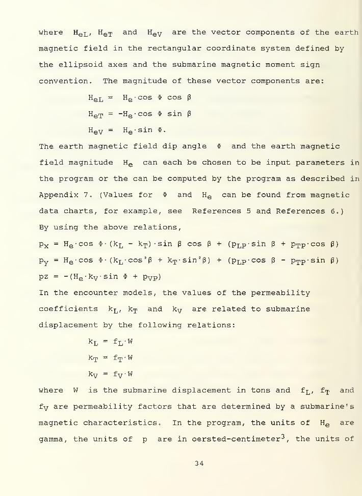
where HeL , HeT and HeV are the vector components of the earth
magnetic field in the rectangular coordinate system defined by
the ellipsoid axes and the submarine magnetic moment sign
convention. The magnitude of these vector components are:
HeL = He cos $ cos (3
HeT = -He -cos § sin (3
HeV = He - sin $.
The earth magnetic field dip angle $ and the earth magnetic
field magnitude He can each be chosen to be input parameters in
the program or the can be computed by the program as described in
Appendix 7. (Values for § and He can be found from magnetic
data charts, for example, see References 5 and References 6.)
By using the above relations,
Px = He -cos $ (Rl - krp) -sin (3 cos (3 + (pLp-sin (3 + pTp-cos (3)
Py = He -cos §-(kL -cos*3 + kT -sin2(3) + (pLp-cos (3 - p^p-sin (3)
pz = -(He -kv -sin $ + pvp )
In the encounter models, the values of the permeability
coefficients kL , kp and kv are related to submarine
displacement by the following relations:
kL = fL -W
kip = fT • w
kv = fv -w
where W is the submarine displacement in tons and f^, f-p and
fy are permeability factors that are determined by a submarine's
magnetic characteristics . In the program, the units of He are
gamma, the units of p are in oersted-centimeter 3, the units of
34

k are oersted-centimeter 3/gamma and the units of f are
oersted-centimeter 3/gamma-ton. If the units of He were
gamma, but the units of p were gamma-foot 3, then the units of
k would be foot 3 and the units of f would be foot 3/ton. To
convert p in gamma-foot 3 to oersted-centimeter 3 or k in
foot 3 to oersted-centimeter 3/gamma or f in foot 3/ton to
oersted-centimeter3/gamma-ton, divide by 3.53. (The program
default values for f-^, fip and fy are values from Reference 1
in foot 3/ton that have been divided by 3.53 to give values in
oersted-centimeter 3/gamma-ton. ) To convert p in weber-meter to
oersted-centimeter 3, multiply by [ 1/ (4 • it) ]
• 10 10 and to convert
p in ampere-centimeter 2 to oersted-centimeter 3, multiply by
1-10 3.
35

Appendix 7 . The Earth Magnetic Field and Dip Angle
An auxiliary magnetic field model is described in this
appendix. The model is the basis for a default choice for either
the value of the earth magnetic field magnitude parameter He or
the earth magnetic field dip angle parameter <$. Relative to
encounter model accuracy, the default values should be addeguate
in most cases.
In the model, the earth magnetic field is generated by a
magnetic dipole that is located at the earth's center and the
earth is a nonmagnetic sphere of radius re . With pe the
magnitude of the dipole moment, the magnitude of the earth field
at a point is
He - (He -He)* - (c-pe/r3
) (3-cos 2 9 + 1)4
where 9 is the polar angle of the point in a spherical
coordinate system and c is a constant whose value is determined
by the choice of units. The dipole moment is coincident with and
in the direction of the polar axis which is directed toward the
earth's southern hemisphere. In this coordinate system, at any
point on the surface of the earth:
He = Heo - (3cos 2 9 + 1)
i
where Heo is the value of He at the magnetic eguator which is
defined by the points on the earth where 6 = 90°. In terms of
the dip angle, at any point on the earth's surface:
He = 2-Heo - (3-cos*$ + 1)""*.
This expression can be obtained by noting that $ can be
36
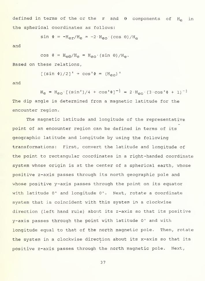
defined in terms of the or the r and 9 components of He in
the spherical coordinates as follows:
sin $ = -Her/He = -2Heo (cos 8)/He
and
cos § = HeQ/He = Heo - (sin 9)/He .
Based on these relations,
[(sin $)/2]2 + cos 2
$ = (Heo )
2
and
He = Heo -[ (sin
2)/4 + cos 2 $]~2 = 2
•
H
eo • (3• cos 2
§ + 1)~*
The dip angle is determined from a magnetic latitude for the
encounter region.
The magnetic latitude and longitude of the representative
point of an encounter region can be defined in terms of its
geographic latitude and longitude by using the following
transformations: First, convert the latitude and longitude of
the point to rectangular coordinates in a right-handed coordinate
system whose origin is at the center of a spherical earth, whose
positive z-axis passes through its north geographic pole and
whose positive y-axis passes through the point on its equator
with latitude 0° and longitude 0°. Next, rotate a coordinate
system that is coincident with this system in a clockwise
direction (left hand rule) about its z-axis so that its positive
y-axis passes through the point with latitude 0° and with
longitude equal to that of the north magnetic pole. Then, rotate
the system in a clockwise direction about its x-axis so that its
positive z-axis passes through the north magnetic pole. Next,
37
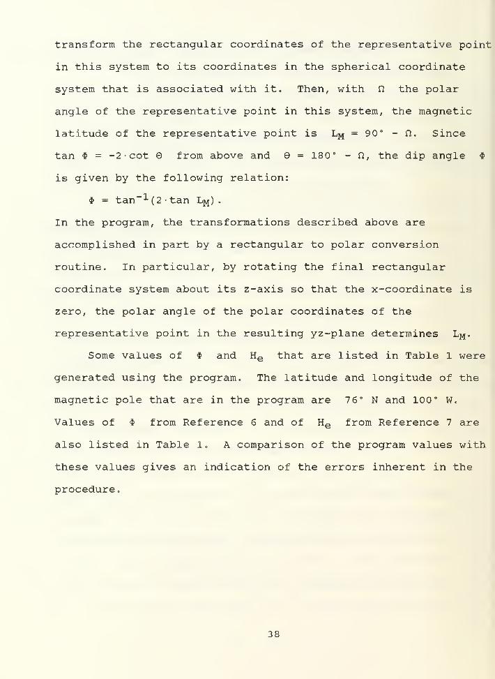
transform the rectangular coordinates of the representative point
in this system to its coordinates in the spherical coordinate
system that is associated with it. Then, with n the polar
angle of the representative point in this system, the magnetic
latitude of the representative point is LM = 90° - n. Since
tan $ = -2• cot 9 from above and 9 = 180° - Q, the dip angle $
is given by the following relation:
§ = tan" 1 (2 -tan L^) .
In the program, the transformations described above are
accomplished in part by a rectangular to polar conversion
routine. In particular, by rotating the final rectangular
coordinate system about its z-axis so that the x-coordinate is
zero, the polar angle of the polar coordinates of the
representative point in the resulting yz-plane determines LM .
Some values of $ and He that are listed in Table 1 were
generated using the program. The latitude and longitude of the
magnetic pole that are in the program are 76° N and 100° W.
Values of $ from Reference 6 and of He from Reference 7 are
also listed in Table 1. A comparison of the program values with
these values gives an indication of the errors inherent in the
procedure.
38
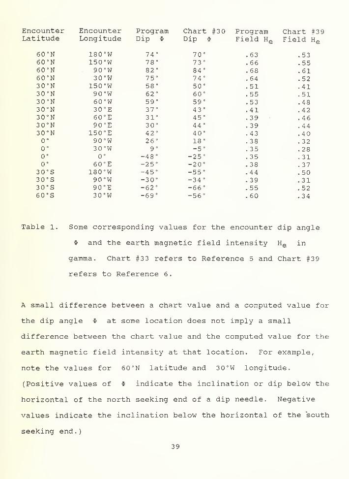
Encounter Encounter Program Chart #3 Program Chart #39Latitude Longitude Dip $ Dip $ Field He Field He
60°N 180°W 74° 70° .63 .5360°N 150°W 78° 73° .66 .5560°N 90°W 82° 84° .68 .6160°N 30°W 75° 74° .64 .5230°N 150°W 58° 50° .51 .4130°N 90°W 62° 60° .55 .5130°N 60°W 59° 59° .53 .4830°N 30°E 37° 43° .41 .4230°N 60°E 31° 45° .39 .4630°N 90°E 30° 44° .39 .4430°N 150°E 42° 40° .43 .400° 90°W 26° 18° .38 .320° 30°W 9° -5° .35 .280° 0° -48° -25° .35 .310° 60°E -25° -20° .38 .37
30°S 180°W -45° -55° .44 .5030°S 90°W -30° -34° .39 .3130°S 90°E -62° -66° .55 .5260°S 30°W -69° -56° .60 .34
Table 1. Some corresponding values for the encounter dip angle
$ and the earth magnetic field intensity He in
gamma. Chart #3 3 refers to Reference 5 and Chart #3 9
refers to Reference 6.
A small difference between a chart value and a computed value for
the dip angle $ at some location does not imply a small
difference between the chart value and the computed value for the
earth magnetic field intensity at that location. For example,
note the values for 60 °N latitude and 30 °W longitude.
(Positive values of $ indicate the inclination or dip below the
horizontal of the north seeking end of a dip needle. Negative
values indicate the inclination below the horizontal of the south
seeking end.
)
39
An extension of the above procedure can be made for finding
the magnetic variation at a location. However, the values
generated by using the procedure are generally unsatisfactory.
Magnetic variation values are charted in Reference 7.
40
Appendix 8. An Alternative Encounter Model
The alternative model that is referred to in Section III is
described in more detail in this appendix. In the model, the
detection range is the slant range R at the CPA for an
encounter with a specified detection probability (usually .5) is
defined by:
R = [c-p/Hs ]V3
where c and p are defined in Appendix 3 and Hs represents
a minimum detectable average magnetic signal that is defined by:
Hs = (ORF) -NM
where ORF is a signal-to-noise ratio called the operator
recognition factor and NM represents the magnetic noise.
Combining these two relations gives:
R = (c-p/[(ORF) •NM ]}1/3.
The value for ORF depends both on the specified detection
probability and on a specified or implied false alarm
probability.
The Anderson formulation is consistent with these relations
in an approximate sense if the average magnetic signal H is
defined as a root mean sguare value such that H = (c-p/R 3) k
and k is an encounter parameter defined by:
k = (2 [S Aj-Fj (Pi) ]
2 H
where the first sum index i = 1, 2, • • •, m and the second sum
index j = 0, 1, 2. For a particular encounter geometry, k is
constant and this suggests that the two encounter models could be
used to determine an average value for k for an encounter
41
region based on average submarine magnetic characteristics.
Values for both k and H are generated by the program and such
values can give an indication of the magnitude of the differences
in detection range estimates that are based on this model and
either of the other two encounter models. A more detailed
comparison of these encounter models is described in Reference 8
.
42
Appendix 9 . An Example of the Program Output
The program is designed to generate the following
quantities: encounter parameter values, lateral range function
values for the crosscorrelation encounter model and for the
square law encounter model, average magnetic signal values, slant
range at CPA values, encounter parameter values and magnetic
signal values. These values can be saved as a program data file
and/or they can be printed.
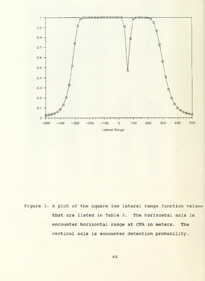
An example of the program's printed output is listed in
Table 2, Table 3 and Table 4. Figure 3 is a plot of the lateral
range function values (a lateral range curve) for the square law
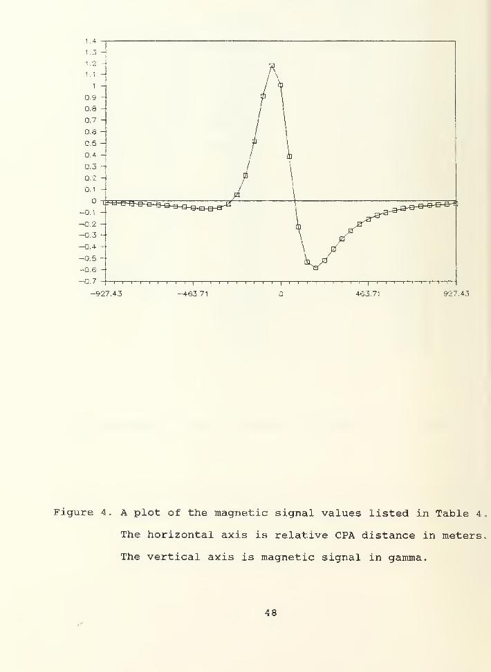
detector that are listed in Table 3. Figure 4 is a plot of the
magnetic signal values that are listed in Table 4.
43
program file name MAD.BASprogram data file name data. madmagnetic data file name data. magprocessing data file name data. prokinematic data file name data. kincombined magnetic, processing & kinematic data file name data.mpkencounter latitude (decimal degrees) 45encounter longitude (decimal degrees) -45encounter variation (decimal degrees) -25encounter dip angle (decimal degrees) 68.41608encounter magnetic field intensity (gamma) 59035.05target permanent longitudinal moment (oersted-cm3)target permanent transverse moment (oersted-cm3)target permanent vertical moment (oersted-cm3
)
target displacement (tons) 1800target longitudinal permeability coefficient 13140target transverse permeability coefficient 2880target vertical permeability coefficient 2880target longitudinal permeability factor 7.3target transverse permeability factor 1.6target vertical permeability factor 1.6sampling period (seconds) .5integration time (seconds) 20adjusted integration time (seconds) 20.5number of samples per encounter 41magnetometer course (decimal degrees) 290magnetometer speed (knots) 180magnetometer altitude (meters) 100target course (decimal degrees) 20target speed (knots) 10target depth (meters) 100magnetometer relative magnetic course (decimal degrees) 311.8202magnetometer relatiive speed (knots) 180.2776magnetometer-target vertical separation (meters) 200target induced longitudinal dipole moment (oersted-cm3 ) 2.017796E+08target induced transverse dipole moment (oersted-cm3) -4 . 422566E+07target induced vertical dipole moment (oersted-cm3 ) 1.58099E+08target dipole moment (oersted-cm3
)
2.601273E+08target dipole moment azimuth (decimal degrees) 32.63751target dipole moment depression (decimal degrees) 37.42884distance between samples on the relative track (meters) 46.37141false alarm rate (false alarms per hour) 3
false alarm probability 1.666667E-02magnetic noise (gamma) .35maximum lateral range (meters) 500lateral range step (meters) 20number of lateral range function values 51
Table 2. An example of a encounter parameter values printout.
44
data. mad lateral range function values
L p(cc) p(sl) H R kmeters gamma meters
-500 .2155959 .0255824 .184247 538. 5165 2.818488-480 . 2721803 .029692 .21034 520 2 . 879916-460 .3464673 3.582633E- 02 .2410144 501. 5974 2 . 943744-440 .4415205 4.529992E- 02 .2785504 483. 3218 3.009938-420 .5573696 6.047795E-02 .3231911 465. 1881 3 . 078418-400 .6872897 .0856887 . 3764825 447. 2136 3 . 149025-380 .8146549 .1287804 .4404623 429. 4182 3.221497-360 .9159235 .2030898 .5177304 411. 8252 3.29544-340 .9745625 . 3272475 .6108596 394. 4617 3 . 370274-320 .9958122 .5141411 .7233319 377. 3593 3 . 445185-300 .9997211 .7388175 .8597726 360. 5551 3 . 519032-280 .9999951 .9177597 1.025158 344. 093 3.590261-260 1 .9896971 1.224529 328. 0244 3 .656775-240 1 .999714 1.463644 312. 41 3.71578-220 1 .9999992 1.74981 297. 3214 3 .763606-200 1 1 2.085394 282. 8427 3.795517-180 1 1 2.470496 269. 0725 3.805514-160 1 1 2.901352 256. 125 3 .786234-140 1 1 3.359555 244. 1311 3 . 72898-120 1 1 3.819509 233. 2381 3. 624058-100 1 1 4.239317 223. 6068 3 . 461596-80 1 1 4.532758 215. 4066 3 . 232958-60 1 1 4.618943 208. 8061 2.932828-40 1 1 4.44342 203. 9608 2.5617-20 1 1 3.97739 200.,9975 2. 128285
1 1 3.332139 200 1.65169720 1 .9999993 2.540665 200..9975 1.16558140 .9999931 .908713 1.76834 203 ..9608 .739417160 .9933111 .467368 1. 110188 208.,8061 . 563718380 .9998733 .7874625 .9039734 215,,4066 .7782836100 .9999999 .9856169 1.086971 223,.6068 1. 134662120 1 .9992399 1.254863 233,.2381 1.490748140 1 .9998478 1.308583 244 .1311 1.811734160 1 .9998431 1.29482 256 .125 2. 089946180 1 .9994995 1.230946 269 .0725 2.326072200 1 .9974561 1.131703 282 .8427 2.523877220 1 .9872744 1.017684 297 .3214 2.688154240 .999999 .9510013 .9018685 312 .41 2.823785260 .9999747 .8646194 .7917129 328 .0244 2.935307280 .9996544 .7242736 .6909791 344 .093 3.026728300 .9973592 .5582789 .6011183 360 .5551 3.10149320 .9876337 .4037092 .5222269 377 .3593 3.162495340 .9608865 .2816961 .4536729 394 .4617 3.212155360 ~ .9086407 .1948741 .3944811 411 .8252 3.252463380 .8301703 .1365131 .3443362 429 .4182 3 . 285058400 .7333605 9.820431E--02 .3014853 447 .2136 3.311281420 .6299387 .0731037 .2645045 465 . 1881 3 . 332228
440 .5302704 5.646636E--02 .2325951 483 .3218 3 . 348799
460 .4408869 4.522933E--02 .205043 501 .5974 3 . 361725
480 . 3645446 3 .747106E--02 . 1812233 520 3. 371603
500 .3013791 3.199235E--02 .1605954 538 .5165 3.378925
Table 3. An example of a lateral range function values printout,
The heading for the crosscorrelation values is p(cc)
and the heading for the square law values is p(sl).
45
0.9 -
0.8 -
0.7 -
aoaaaaoaaaaGq ^aa qa^
I
i—i—i—i—|—i—i—i—i—|—i—i—i—i—|—i—i—i—i—|—i—i—i—i—|—i—i—i—i—|—i—i—i—i—|—i—i—i—i—|—i—i—i—i—I—i
i i r
-500 -400 -300 -200 -100 100 200 300 400 500
Lateral Range
Figure 3 . A plot of the square law lateral range function values
that are listed in Table 3. The horizontal axis is
encounter horizontal range at CPA in meters. The
vertical axis is encounter detection probability.
46
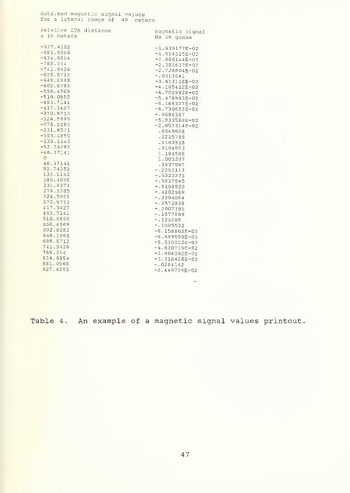
data. mad magnetic signal valuesfor a lateral range of 40 meters
relative CPA distance magnetic signals in meters Hs in gamma
-927.4282 -1 . 619177E-02-881.0568 -1.834315E-02-834.6854 -2 . 086144E-02-788.314 -2. 381637E-02-741.9426 -2.728804E-02-695.5712 -.0313641-649.1998 -3.613118E-02-602.8283 -4.165412E-02-556.4569 -4 . 792992E-02-510.0855 -5.478963E-02-463.7141 -6. 169327E-02-417.3427 -6.730653E-02"370.9713 -.0686387-324.5999 -5 . 933568E-02-278.2285 -2 . 6523 14E-02-231.8571 .0540608-185.4856 .2215785"139.1142 .5163918-92.74282 .9104893-46.37141 1.184586
1.00320746.37141 .383706792.74282 -.2252113139.1142 -.5323231185.4856 -.5837545231.8571 -.5168925278.2285 -.4202569324.5999 -.3304064370.9713 -.2572838417.3427 -.2007385463.7141 -.1577988510.0855 -.125285556.4569 -.1005532602.8283 -8.158605E-02649.1998 -6.689598E-02695.5712 -5.539922E-02741.9426 -4.630719E-02788.314 -3.904362E-02834.6854 -3 . 3 18428E-02881.0568 -.0284142927.4282 -2 . 449729E-02
Table 4. An example of a magnetic signal values printout
47
1.4
1.3 -
1.2 -
1.1
1
Q.9 -
D.8 -
0.7 -
0.6
0.5 -
0.4
0.3 -
0.2 -
0.1 -
-0.1 -
-0 2 -
-0.3 -
-0.4 -
-0.5
-0.6 -
-0.7
tm^^e-SHEHEHE>-EH3.
T 1 1 1 1 1 1 1 1
1
1
-927.43 -463.71
~i—i—i—i—i—|—i—i—r- i—i—i—i—i—i—
r
463.71 927.43
Figure 4. A plot of the magnetic signal values listed in Table 4
The horizontal axis is relative CPA distance in meters
The vertical axis is magnetic signal in gamma.
48
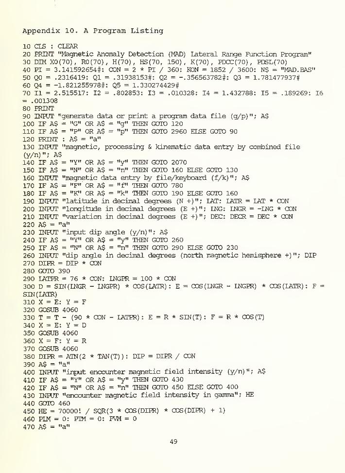
Appendix 10. A Program Listing
10 CLS : CLEAR20 PRINT "Magnetic Anomaly Detection (MAD) lateral Range Function Program ,,
30 DTMX0(70), R0(70), H(70) , HS(70, 150), K(70) , PDCC(70) , PDSL(70)40 PI = 3. 141592654 #: CON = 2 * PI / 360: KON = 1852 / 3600: N$ = "MAD.BAS"50 Q0 = .2316419: Ql = .31938153#: Q2 = -.356563782#: Q3 = 1.781477937#60 Q4 = -1.821255978#: Q5 = 1.330274429#70 II = 2.515517: 12 = .802853: 13 = .010328: 14 = 1.432788: 15 = .189269: 16= .00130880 PRINT90 INPUT "generate data or print a program data file (g/p)"; A$100 IF A$ = "G" OR A$ = "g" THEN GOTO 120110 IF A$ = "P" OR A$ = "p" THEN GOTO 2960 ELSE GOTO 90120 PRINT : A$ = "a"
130 INPUT "magnetic, processing & kinematic data entry by combined file(y/n)"; A$140 IF A$ = "Y" OR A$ = "y" THEN GOTO 2070150 IF A$ = "N" OR A$ = "n" THEN GOTO 160 ELSE GOTO 130160 INPUT "magnetic data entry by file/keyboard (f/k)"; A$170 IF A$ = "F" OR A$ = "f" THEN GOTO 780180 IF A$ = "K" OR A$ = "k" THEN GOTO 190 ELSE GOTO 160190 INPUT "latitude in decimal degrees (N +)"; IAT: IATR = IAT * CON200 INPUT "longitude in decimal degrees (E +)"; LNG: LNGR = -LNG * CON210 INPUT "variation in decimal degrees (E +)"; DEC: DECR = DEC * CON220 A$ = "a"230 INPUT "input dip angle (y/n)"; A$240 IF A$ = "Y" OR A$ = "y" THEN GOTO 260250 IF A$ = "N" OR A$ = "n" THEN GOTO 290 ELSE GOTO 230260 INPUT "dip angle in decimal degrees (north magnetic hemisphere +) " ; DIP270 DIPR = DIP * CON280 GOTO 390290 LATPR = 76 * CON: LNGPR = 100 * CON300 D = SIN(LNGR - LNGPR) * COS (IATR) : E = COS (LNGR - LNGPR) * COS (IATR) : F =
SIN (IATR)
310 X = E: Y = F320 GOSUB 4060330 T = T - (90 * CON - LATPR) : E = R * SIN(T) : F = R * COS(T)
340 X = E: Y = D350 GOSUB 4060360 X = F: Y = R370 GOSUB 4060380 DIPR = ATN(2 * TAN(T) ) : DIP = DIPR / CON390 A$ = "a"
400 INPUT "input encounter magnetic field intensity (y/n)"; A$
410 IF A$ = "Y" OR A$ = "y" THEN GOTO 430
420 IF A$ = "N" OR A$ = "n" THEN GOTO 450 ELSE GOTO 400
430 INPUT "encounter magnetic field intensity in gamma"; HE440 GOTO 460450 HE = 70000! / SQR(3 * COS (DIPR) * COS (DIPR) + 1)
460 PIM = 0: PTM = 0: PVM =470 A$ = "a"
49
480 INHJT "input target permanent dipole moments (y/n) " ; A$490 IF A$ = "Y" OR A$ = "y" THEN GOTO 510500 IF A$ = "N" OR A$ = "n" THEN GOTO 540 ELSE GOTO 480510 INHJT "permanent longitudinal moment in oersted-cm3 (stern-to-bow +)"; ELM520 INHJr "permanent transverse moment in oersted-cm3 (port-to-starboard +) "
;
ETM530 INHJT "permanent vertical moment in oersted-cnG (downward +) " ; FVM540 INHJT "target displacement in tons"; WT550 A$ = "a"560 INHJT "input target permeability coefficients or factors (c/f)"; A$570 IF A$ = "C" OR A$ = "c" THEN GOTO 590580 IF A$ = "F" OR A$ = "f" THEN GOTO 630 ELSE GOTO 560590 INHJT "longitudinal permeability coefficient in cgs units"; KL600 INHTT "transverse permeability coefficient in cgs units"; KT610 INHJT "vertical permeability coefficient in cgs units"; KV620 FL = KL / WT? FT = KT / WT: FV = KV / WT: GOTO 710630 INHTT "longitudinal displacement factor in cgs units"; FL640 INHTT "transverse displacement factor in cgs units"; FT650 INHJT "vertical displacement factor in cgs units"; FV660 KL = FL * WT: KT = FT * WT: KV = FV * WT670 A$ - "a"680 INHJT "generate a magnetic data file (y/n)"; A$690 IF A$ = "Y BC OR A$ = "y" THEN GOTO 710700 IF A$ - "N" OR A$ = "n" THEN GOTO -850 ELSE GOTO 680710 INHJT "magnetic data file name"; M$720 ON ERROR GOTO 730: GOTO 740730 RESUME 710740 OEEN "0'\ #1, M$750 WRITE #1, LAT, LNG, DEC, DIE, HE, ELM, ETM, FVM, WT, KL, KT, KV, FL, FT,
FV760 CLOSE770 GOTO 850780 INHJT "magnetic data file name"; M$790 ON ERROR GOTO 800: GOTO 810800 RESUME 780810 OEEN "I", #1, M$820 INHJT #1, LAT, LNG, DEC, DIE, HE, ELM, ETM, EVM, WT, KL, KT, KV, FL, FT,
FV830 CLOSE840 DIFR - DIE * CON850 A$ = "a"860 INHJT "processing data entry by file/keyboard (f/k)"; A$870 IF A$ = "F" OR A$ = "f" THEN GOTO 1450880 IF A$ = "K" OR A$ = "k" THEN GOTO 890 ELSE GOTO 860890 A$ = "a"900 INHJT "input sampling period (y/n)"; A$910 IF A$ = "Y" OR A$ = "y" THEN GOTO 930920 IF A$ = "N" OR A$ = "n" THEN GOTO 960 ELSE GOTO 900930 INHJT "sampling period in seconds"; DT940 IF DT <= THEN FRINT : ERINT "must be greater than zero": FRINT : GOTO930950 GOTO 1090
50
960 A$ = "a"970 INPUT "input maximum magnetic signal frequency (y/n)"; A$980 IF A$ = "Y" OR A$ = "y" THEN GOTO 1000990 IF A$ = "N" OR A$ = "n" THEN GOTO 1030 ELSE GOTO 9701000 INPUT "maximum magnetic signal frequency in Hertz"; MAXF1010 IF MAXF <= THEN PRINT : PRINT "must be greater than zero": PRINT : GOTO10001020 GOTO 10801030 INPUT ''minimum target slant range at CPA in meters"; MINRO1040 IF MINRO <= THEN PRINT : PRINT "must be greater than zero": PRINT :
GOTO 10301050 INPUT "maximum magnetometer relative speed in knots"; MAXVMK1060 MAXVM = MAXVMK * KON: MAXF = 2 * MAXVM / MINRO1070 IF MAXVM <= THEN PRINT : PRINT "must be greater than zero": PRINT :
GOTO 10501080 DT = 1 / (2 * MAXF) : REM low pass filter, Nyquist sampling rate1090 A$ = "a"1100 INPUT "input integration time (y/n)"; A$1110 IF A$ = "Y" OR A$ = "y" THEN GOTO 11301120 IF A$ = "N" OR A$ = "n" THEN GOTO 1210 EISE GOTO 11001130 INPUT "integration time in seconds"; IT1140 IF IT >= DT THEN GOTO 11701150 PRINT : PRINT "IT = " + STR$(TT) + " seconds - iiujiimum = " + STR$(DT) + "
seconds": PRINT1160 GOTO 11301170 NS = 2 * INT(rT / EXT / 2) + 1: REM adj number of samples per integrationtime1180 IF NS <= 151 THEN GOTO 13401190 PRINT : PRINT "TT = " + STR$(TT) + " seconds - maximum = " + STR$(150 *
DT) + " seconds": PRINT1200 GOTO 11301210 INPUT "maximum target slant range at CPA in meters"; MAXR01220 IF MAXR0 <= THEN PRINT : PRINT "must be greater than zero": PRINT :
GOTO 12101230 INPUT "minimum magnetometer relative speed in knots"; MTNVMK1240 MINVM = MINVMK * KON1250 IF MINVM <= THEN PRINT : PRINT "must be greater than zero": PRINT :
GOTO 12301260 IT = 2 * MAXR0 / MINVM1270 IF IT >= DT THEN GOTO 13001280 PRINT : PRINT "IT = " + STR$(TT) + " seconds - minimum = " + STR$(DT) + "
seconds": PRINT1290 GOTO 11001300 NS = 2 * INT(rT / DT / 2) +1: REM adjusted number of samples perintegration time1310 IF NS <= 151 THEN GOTO 1340
1320 PRINT : PRINT "IT = " + STR$(TT) + " seconds - mmiinum = " + STR$(150 *
DT) + " seconds": PRINT1330 GOTO 11001340 A$ = "a"1350 INPUT "generate a processing data file (y/n)"; A$
1360 IF A$ = "Y" OR A$ = "y" THEN GOTO 1380
51
1370 IF A$ = "N" OR A$ = "n" THEN GOTO 1510 ELSE GOTO 13501380 INHJT "processing data file name"; P$1390 ON ERROR GOTO 1400: GOTO 14101400 RESUME 13801410 OPEN "O", #1, P$1420 WRITE #1, DT, IT, NS1430 CLOSE1440 GOTO 15101450 INPUT "processing data file name"; P$1460 ON ERROR GOTO 1470: GOTO 14801470 RESUME 14501480 OPEN "I", #1, P$1490 INPUT #1, DT, IT, NS1500 CLOSE1510 A$ = "a"1520 INPUT "kinematic data entry by file/keyboard (f/k)"; A$1530 IF A$ = "F" OR A$ = "f" THEN GOTO 18901540 IF A$ = "K" OR A$ = "k" THEN GOTO 1550 ELSE GOTO 15101550 INPUT "magnetometer course in decimal degrees (0 if at rest) " ; CM1560 MCM = (CM - DEC) : MCMR = MCM * CON: REM magnetometer magnetic course1570 INPUT "magnetometer speed in knots"; VMK1580 INPUT "magnetometer altitude in meters (below is -)"; AM1590 INPUT "target course in decimal degrees"; CT1600 MCT = (CT - DEC) : MCTR = MCT * CON: REM target magnetic course1610 INPUT "target speed in knots"; VTK1620 INPUT "target depth in meters (above is -) " ; AT1630 IIM - KL * HE * COS(DIPR) * COS(MCTR) : ITM = -KT * HE * COS(DIPR) *
SIN (MCTR)1640 IVM = KV * HE * SIN(DIFR)1650 DMX = (PIM + IIM) * SIN (MCTR) + (PTM + ITM) * COS (MCTR)1660 DMY = (PIM + ILM) * COS (MCTR) - (PTM + ITM) * SIN (MCTR)1670 DMV = PVM + IVM1680 X = DMX: Y = DMY1690 GOSUB 40601700 OMLR = T: X = DMV: Y = R1710 GOSUB 40601720 DM = R: OMR = T1730 WXK = VMK * SIN(MCMR) - VTK * SIN(MCTR) : WYK = VMK * COS(MCMR) - VTK *
COS (MCTR)
1740 Z = AM + AT: REM vertical separation (- for magnetometer below target)1750 X = WXK: Y = WYK: GOSUB 40601760 CR = T: WK = R: REM relative magnetometer magnetic course and speed1770 GML = OMIR / CON: CM = OMR / CON: C = CR / CON1780 A$ = "a"1790 INPUT "generate a kinematic data file (y/n)"; A$1800 IF A$ = "Y" OR A$ = "y" THEN GOTO 18201810 IF A$ = "N" OR A$ = "n" THEN GOTO 1950 ELSE GOTO 17901820 INPUT "kinematic data file name"; K$1830 ON ERROR GOTO 1840: GOTO 18501840 RESUME 18201850 OPEN "O", #1, K$1860 WRITE #1, CM, VMK, AM, CT, VTK, AT, Z, C, WK, IIM, ITM, IVM, DM, OML, CM
52
1870 CIDSE1880 GOTO 19501890 INHJT "kinematic data file name"; K$1900 ON ERROR GOTO 1910: GOTO 19201910 RESUME 18901920 OPEN "I", #1, K$1930 INPUT #1, CM, VMK, AM, CT, VTK, AT, Z, C, WK, IIM, TTM, IVM, CM, OML, OM1940 CLOSE1950 A$ = "a"1960 INPUT "generate a combined magnetic, processing & kinematic data file(y/n)"; A$1970 IF A$ = "Y" OR A$ = "y" THEN GOTO 19901980 IF A$ = "N" OR A$ = "n" THEN GOTO 2140 ELSE GOTO 19601990 INPUT "combined magnetic, processing & kinematic data file name"; E$2000 ON ERROR GOTO 2010: GOTO 20202010 RESUME 19902020 OPEN "O", #1, E$2030 WRITE #1, LAT, LNG, DEC, DIP, HE, PLM, PTM, PVM, WT, KL, KT, KV, FL, FT,
FV, DT, IT2040 WRITE #1, NS, CM, VMK, AM, CT, VTK, AT, Z, C, WK, IIM, ITM, IVM, DM, OML,
OM, MS, P$, K$2050 CLOSE2060 GOTO 21402070 INPUT "combined magnetic, processing & kinematic data file name"; E$2080 ON ERROR GOTO 2090: GOTO 21002090 RESUME 20702100 OPEN "I", #1, E$2110 INPUT #1, LAT, LNG, DEC, DIP, HE, PLM, PTM, PVM, WT, KL, KT, KV, FL, FT,
FV, DT, IT2120 INPUT #1, NS, CM, VMK, AM, CT, VTK, AT, Z, C, WK, IIM, ITM, IVM, DM, OML,
OM, MS, P$, K$2130 CLOSE2140 OMLR = OML * CON: OMR = OM * CON: DIPR = DIP * CON2150 CR = C * CON: W = WK * KON2160 INPUT "required false alarm rate in false alarms per hour"; FAR2170 PF = FAR * IT / 3600: REM false alarm probability2180 Y = PF: IF PF > .5 THEN Y = 1 - Y: REM inverse normal approximation2190 Y = SQR(LOG(l / Y / Y)
)
2200 Y = Y - (II + Y * (12 + 13 * Y) ) / (1 + Y * (14 + Y * (15 + 16 * Y) )
)
2210 IF PF < .5 THEN Y = -Y2220 ZP = -Y2230 CHI = NS * (1 - 2 / 9 / NS + ZP * SQR(2 / 9 / NS) ) 3: REM inverse
chi-square approximation2240 INPUT "magnetic noise in gamma"; SIG2250 INPUT "maximum lateral range in meters"; LRM2260 INPUT "lateral range step in meters"; ST2270 IF ST <= LRM THEN GOTO 22902280 PRINT : PRINT "maximum step is " + STR$(LRM) + " meters": PRINT : GOTO
22602290 NC = 2 * INT (LRM /ST) +1: REM number of lateral range function values
2300 IF NC <= 71 THEN GOTO 2320
53
2310 PRINT : PRINT "minimum step is " + STR$(LRM / 35) + " meters": PRINT :
GOTO 22602320 ATT = DT * NS: REM adjusted integration time2330DS=W*DT: REM distance between samples on the relative track2340 X0 = -(NC - 1) / 2 * ST2350 FOR I = TO NC - 1
2360 X0(I) = X02370 X = X0: Y = Z
2380 GOSUB 40602390 RO = R: R0(I) = R: REM target slant range at CPA in meters2400 DELE = T: REM target depression angle complement at CPA in radians2410 IF R0 = THEN GOTO 2730: REM zero lateral range and vertical separation2420 DMF = DM / 10 / R0 " 3: REM dipole moment factor2430 L = OOS(CMR) * COS(CR - OMLR)2440 M = COS(DELR) * COS(OMR) * SIN(CR - OMLR) - SIN(DELR) * SIN(CMR)2450 N = -SIN(DELR) * COS(CMR) * SIN(CR - OMLR) - COS(DELR) * SIN(OMR)2460 LI = OOS(DIPR) * COS(CR)2470 Ml = COS(DELR) * COS(DIPR) * SIN(CR) - SIN(DELR) * SIN(DIPR)2480 Nl = -SIN(DELR) * COS(DIPR) * SIN(CR) - COS(DELR) * SIN(DIPR)2490 A2 = 2*L*L1-M*M1-N*N1: REM Anderson Function Coefficient2500 Al = 3 * (N * LI + L * Nl) : REM Anderson Function Coefficient2510 AO = 2 * N * Nl - L * LI - M * ML: REM Anderson Function Coefficient2520 SUM = 0: HMAX = 0: HMTN =2530 FOR J = TO NS - 1
2540 S = (J - (NS - 1) / 2) * DS: BA = S / R0: REM Anderson Function Argument2550 AF=1/(1 + BA*BA) ' 2*5: REM Anderson Function Factor2560 HSF = (A2 * BA * BA + Al * BA + A0) * AF: REM magnetic signal factor2570 HS(I, J) = DMF * HSF: REM magnetic signal value2580 IF HS(I, J) > HMAX THEN HMAX = HS(I f J)
2590 IF HS(I, J) < HMTN THEN HMIN = HS(I, J)
2600 SUM = SUM + HSF * HSF2610 NEXT J2620 H(I) = HMAX - HMTN2630 K(I) = SQR(SUM)2640 W = -ZP + DMF * SQR(SUM) / SIG2650 LAM = DMF * DMF * SUM / (SIG * SIG) : AA = NS + LAM: BB = 1 + LAM / (NS +LAM)
2660 ZN = -SQR(2 * CHI / BB) + SQR(2 * AA / BB - 1) : X1=W2670 GOSUB 41202680 IF Yl > 1 THEN Yl = 1
2690 PDCC(I) = Yl: XI = ZN2700 GOSUB 41202710 IF Yl > 1 THEN Yl = 1
2720 PDSL(I) = Yl2730 X0 = X0 + ST2740 NEXT I2750 A$ = "a"2760 INPUT "generate a program data file (y/n) " ; A$2770 IF A$ = "Y" OR A$ = "y" THEN GOTO 27902780 IF A$ = "N" OR A$ = "n" THEN GOTO 3120 ELSE GOTO 27602790 INPUT "program data file name"; D$2800 ON ERROR GOTO 2810: GOTO 2820
54
2810 RESUME 27902820 OPEN "0", #1, D$2830 WRITE #1, IAT, LNG, DEC, DIP, HE, PIM, PTM, PVM, WT, KL, KT, KV, FL, FT,FV, DT, IT, AIT2840 WRITE #1, NS, CM, VM, AM, CT, VT, AT, IIM, ITM, IVM, Z, C, W, DM, OML,CM, FAR, PF, SIG, ST2850 WRITE #1, IRM, DS, NC, M$, P$, K$, E$2860 FOR I = TO NC - 1
2870 WRITE #1, X0(I), PDCC(I) , PDSL(I) , K(I) , H(I) , R0(I)2880 NEXT I
2890 FOR I = TO NC - 1
2900 FOR J = TO NS - 1
2910 WRITE #1, HS(I, J)
2920 NEXT J2930 NEXT I
2940 CLOSE2950 GOTO 31202960 INPUT "program data file name"; D$2970 ON ERROR GOTO 2980: GOTO 29902980 RESUME 29602990 OPEN "I", #1, D$3000 INPUT #1, IAT, ING, DEC, DIP, HE, PIM, PTM, PVM, WT, KL, KT, KV, FL, FT,FV, DT, IT, AIT3010 INPUT #1, NS, CM, VM, AM, CT, VT, AT, IIM, ITM, IVM, Z, C, W, DM, OML,CM, FAR, PF, SIG, ST3020 INPUT #1, LRM, DS, NC, M$, P$, K$, E$3030 FOR I = TO NC - 1
3040 INPUT #1, X0(I), PDCC(I), PDSL(I) , K(I) , H(I) , R0(I)3050 NEXT I
3060 FOR I = TO NC - 1
3070 FOR J = TO NS - 1
3080 INPUT #1, HS(I, J)
3090 NEXT J3100 NEXT I
3110 CLOSE3120 PRINT : A$ = "a"3130 INPUT "print encounter parameter values (y/n)"; A$3140 IF A$ = "Y" OR A$ = "y" THEN GOTO 31603150 IF A$ = "N" OR A$ = "n" THEN GOTO 3670 ELSE GOTO 31303160 LPRINT3170 LPRINT "program file name " + N$3180 LPRINT "program data file name " + D$3190 LPRINT "magnetic data file name " + M$3200 LPRINT "processing data file name " + P$3210 LPRINT "kinematic data file name " + K$3220 LPRINT "combined magnetic, processing & kinematic data file name " + E$3230 LPRINT "encounter latitude (decimal degrees) "; SPC(2)
;
IAT3240 LPRINT "encounter longitude (decimal degrees) "; SPC(2) ;
LNG3250 LPRINT "encounter variation (decimal degrees) "; SPC(2)
;
DEC
55
3260 LPRINT '
DIP3270 LPRINT '
HE3280 LPRINT '
PIM3290 LPRINT '
PIM3300 LPRINT '
PVM3310 LPRINT •
WT3320 LPRINT '
KL3330 LPRINT '
KT3340 LPRINT •
KV3350 LPRINT •
FL3360 LPRINT '
FT3370 LPRINT '
FV3380 LPRINT '
DT3390 LPRINT '
IT3400 LPRINT '
ATT3410 LPRINT •
NS3420 LPRINT '
CM3430 LPRINTVMK3440 LPRINT '
AM3450 LPRINTCI3460 LPRINT •
VTK3470 LPRINTAT3480 LPRINT '
C3490 LPRINT '
WK3500 LPRINT •
Z
3510 LPRINT '
IIM
'encounter dip angle (decimal degrees)
'encounter magnetic field intensity (gamma)
'target permanent longitudinal moment (oersted-cm3)
•target permanent transverse moment (oersted-cm3)
'target permanent vertical moment (oersted-cm3)
'target displacement (tons)
'target longitudinal permeability coefficient
•target transverse permeability coefficient
'target vertical permeability coefficient
'target longitudinal permeability factor
'target transverse permeability factor
'target vertical permeability factor
'sampling period (seconds)
'integration time (seconds)
'adjusted integration time (seconds)
'number of samples per encounter
•magnetometer course (decimal degrees)
•magnetometer speed (knots)
•magnetometer altitude (meters)
'target course (decimal degrees)
'target speed (knots)
'target depth (meters)
•magnetometer relative magnetic course (decimal degrees)
•magnetometer relative speed (knots) "
•magnetometer-target vertical separation (meters)
'target induced longitudinal dipole moment (oersted-cm3
)
56
3520 LPRINT "target induced transverse dipole moment (oersted-cm3) "; SPC(2ITM3530 LPRINT "target induced vertical dipole moment (oersted-cm3) "; SPC(2IVM3540 LPRINT "target dipole moment (oersted-cm3) "; SPC(2EM3550 LPRINT "target dipole moment azimuth (decimal degrees) "; SPC(2OML3560 LPRINT "target dipole moment depression (decimal degrees) "; SPC(2CM3570 LPRINT "distance between samples on the relative track (meters)"; SPC(2DS3580 LPRINT "false alarm rate (false alarms per hour) "; SPC(2FAR3590 LPRINT "false alarm probability "; SPC(2PF3600 LPRINT "magnetic noise (gamma) "; SPC(2SIG3610 LPRINT "maximum lateral range (meters) "; SPC(2LRM3620 LPRINT "lateral range step (meters) "; SPC(2ST3630 LPRINT "number of lateral range function values "; SPC(2NC3640 FOR I = TO 153650 LPRINT3660 NEXT I
3670 PRINT : A$ = "a"3680 INPUT "print lateral range function values (y/n)"; A$3690 IF A$ = "Y" OR A$ = "y" THEN GOTO 37103700 IF A$ = "N" OR A$ = "n" THEN GOTO 3790 ELSE GOTO 36803710 LPRINT D$; " lateral range function values"3720 LPRINT : LPRINT3730 LPRINT "L P(cc) P(sl) H R
k"3740 LPRINT "meters gamma meters"
3750 LPRINT3760 FOR I = TO NC - 1
3770 LPRINT X0(I) ; TAB(10) ; PDCC(I) ; TAB(24) ; PDSL(I) ; TAB(38) ; H(I) ; TAB(52) ?
R0(I) ; TAB(70) ; K(I)
3780 NEXT I
3790 PRINT : A$ = "a"
3800 INPUT "print magnetic signal values (y/n)"; A$3810 IF A$ = "Y" OR A$ = "y" THEN GOTO 3830
3820 IF A$ = "N" OR A$ = "n" THEN GOTO 4010 ELSE GOTO 3800
3830 PRINT : PRINT "identify signal by encounter lateral range index"
3840 PRINT "lateral range equals the index times " + STR$(ST) + " meters"
3850 PRINT "index values: -" + STR$((NC - 1) / 2) + " to " + STR$((NC - 1) /
2)
3860 INPUT "lateral range index"; K: I = K + (NC - 1) / 2
3870 LPRINT : LPRINT : LPRINT3880 LPRINT D$; " magnetic signal values"
57
3890 LPRINT "for a lateral range of "; K * ST; " meters"3900 LPRINT3910 LPRINT "relative CPA distance"; TAB(35) ; "magnetic signal"3920 LPRINT "s in meters"; TAB(35) ; "Hs in gamma"3930 LPRINT3940 FOR J = TO NS - 1
3950 LPRINT (J - (NS - 1) / 2) * DS; TAB(35) ; HS(I, J)
3960 NEXT J3970 PRINT : A$ = "a"3980 INPOT "print magnetic signal values for a different lateral range (y/n)
"
A$3990 IF A$ = "Y" OR A$ = "y" THEN GOTO 38304000 IF A$ = "N" OR A$ = "n" THEN GOTO 4010 ELSE GOTO 39804010 PRINT : A$ = "a"
4020 INPUT "continue to use the program (y/n) " ; A$4030 IF A$ = "Y" OR A$ = "y" THEN GOTO 104040 IF A$ = "N" OR A$ = "n" THEN GOTO 4050 ELSE GOTO 40204050 END4060 R = SQR(X * X + Y * Y) : REM rectangular to polar conversion4070 IF R = THEN T = 0: RETURN4080 IF ABS(X / R) = 1 THEN Q = SGN(X) * (PI / 2) ELSE Q = ATN(X / R / SQR(1X * X / R / R)
)
4090 IF ABS(Y / R) = 1 THEN T = (PI / 2) * (1 - SGN(Y)) ELSE T = (PI / 2) -
ATN(Y / R / SQR(1 -Y*Y/R/R))4100 IF Q < THEN T = 2 * PI - T4110 RETURN4120 Yl - XI: IF XI < THEN Yl = -Yl: REM normal approximation4130 G = 1 / (1 + Q0 * Yl)
4140 Yl = EXP(-Y1 * Yl / 2) / SQR(2 * PI) * G * (Ql + G * (Q2 + G * (Q3 + G *
(Q4 + G * Q5) ) )
)
4150 IF XI >= THEN Yl = 1 - Yl4160 RETURN
58
References
1. "Mad Signal Processing Study," C2-61009-2, Texas Instruments,Inc., Dallas, Texas, April 1961.
2. Handbook of Mathematical Functions , National Bureau ofStandards, Applied Mathematics Series 55, Washington, D.C. , June1964.
3. "Magnetic Airborne Detector Program," Summary TechnicalReport of Division 6, National Defense Research Committee,Vol. 5, Washington, D.C, 1946.
4. Anderson, J. E., "Magnetic Airborne Detection FreguencyResponses," NADC-EL-47-50 , Naval Air Development Center,Johnsville, PA, October 1949.
5. "Magnetic Inclination or Dip, EPOCH 1975.0," Chart Number 33,
9th Edition, Defense Mapping Agency Hydrographic Center,Washington, DC 20390, November 1975.
6. "Total Intensity of the Earth's Magnetic Field, EPOCH 1975.0,"Chart Number 39, 4th Edition, Defense Mapping Agency HydrographicCenter, Washington, DC 20390, December 1975.
7. "Magnetic Variation, EPOCH 1975.0," Chart Number 33, 7thEdition, Defense Mapping Agency Hydrographic Center, Washington,DC 20390, June 1975.
8. Schluckebier, D. C. , "A Comparison of Three Magnetic AnomalyDetection (MAD) Models," Thesis, Naval Postgraduate School,March 1984.
59

Initial Distribution List
Copies
Director of Research Administration (Code 012) 1
Naval Postgraduate SchoolMonterey, CA 93943-5000
Defense Technical Information Center 2
Cameron StationAlexandria, VA 22314
Library (Code 0142) 2
Naval Postgraduate SchoolMonterey, CA 93943-5000
Commander 1
Submarine Development Squadron 12Naval Submarine Base, New LondonGroton, CT 06349
Commander 1
Surface Warfare Development GroupNaval Amphibious Base, Little CreekNorfolk, VA 23521
Naval Air Development Center 1
Johnsville, PA 18974
Naval Surface Weapons Center 1
White OakSilver Spring, MD 20910
Naval Underwater Systems Center 1
Newport, RI 02840
Naval Underwater Systems Center 1
New London, CT 063 2
Naval Technical Intelligence Center 1
4301 Suitland RoadWashington, D. C. 20390
Naval Research Laboratory 1
Washington, D. C. 20375
Center for Naval Analysis 1
44 01 Ford AvenueP. O. Box 16268Alexandria, VA 22302-0268

Naval Ocean Systems Center 1San Diego, CA 92132
Naval Postgraduate SchoolMonterey, CA 93943-5000Code 55Fo 30


DUDLEY KNOX LIBRARY
3 2768 00302620 4


![Execution Time Minimization Based on Hardware/Software ...compute the probabilities to reach any hardware module, based on pro ling information [8]. This algorithm can be applied only](https://img.pdfslide.net/doc/110x75/5e92b85c9737c177390e8486/execution-time-minimization-based-on-hardwaresoftware-compute-the-probabilities.jpg)

![Archimedes: Efficient Query Processing over Probabilistic ...edge from existing KBs [5], query-driven inference to compute probabilities of the query facts [35], and the UDA-GISTframeworkforin-databasedata-paralleland](https://img.pdfslide.net/doc/110x75/5f48edeb5760ae07f21c4770/archimedes-eficient-query-processing-over-probabilistic-edge-from-existing.jpg)