A proximal bundle method for nonsmooth nonconvex functions

Computational Optimization and Applications manuscript No.(will be inserted by the editor)

A proximal bundle method for nonsmooth nonconvexfunctions with inexact information

W. Hare · C. Sagastizabal · M. Solodov

Received: date / Accepted: date

Abstract For a class of nonconvex nonsmooth functions, we consider the problem of com-puting an approximate critical point, in the case when only inexact information about thefunction and subgradient values is available. We assume that the errors in function and sub-gradient evaluations are merely bounded, and in principle need not vanish in the limit. Weexamine the redistributed proximal bundle approach in this setting, and show that reasonableconvergence properties are obtained. We further consider a battery of difficult nonsmoothnonconvex problems, made even more difficult by introducing inexactness in the availableinformation. We verify that very satisfactory outcomes are obtained in our computationalimplementation of the inexact algorithm.

Keywords nonsmooth optimization · nonconvex optimization · bundle method · inexactinformation · locally Lipschitz functions · proximal point.

Mathematics Subject Classification (2010) 90C25 · 49J52 · 65K10 · 49M05.

Research of the first author is supported in part by NSERC DG program and UBC IRF. The second au-thor is supported by CNPq 303840/2011-0, AFOSR FA9550-08-1-0370, NSF DMS 0707205, PRONEX-Optimization, and FAPERJ. The third author is supported in part by CNPq Grant 302637/2011-7, PRONEX-Optimization, and by FAPERJ.

W. HareUniversity of British Columbia, Okanagan Campus, 3333 University Way, Kelowna, BC, V1Y 8C5, Canada.E-mail: [email protected]

C. Sagastizabalvisiting researcher at IMPA, Estrada Dona Castorina 110, Jardim Botanico, Rio de Janeiro RJ 22460-320,Brazil.E-mail: [email protected]

M. SolodovIMPA – Instituto de Matematica Pura e Aplicada,Estrada Dona Castorina 110, Jardim Botanico, Rio de Janeiro, RJ 22460-320, Brazil.E-mail: [email protected]

2 Hare, Sagastizabal, and Solodov

1 Introduction

In this paper we seek to approximately solve the problem

min f (x) : x ∈ D, (1)

where f : IRn → IR is a locally Lipschitz function and D ⊂ IRn is a convex compact set.The information at disposal is provided by an inexact procedure that, given a point xi,

returns some estimations for the function value at xi and for one subgradient at xi. Accord-ingly, the available information is f i ≈ f (xi) and gi ≈ g(xi) ∈ ∂ f (xi). Working with inexactinformation presents a natural challenge in a number of modern applications. In this paper,we shall assume that the inexact information is provided in a manner such that the errorsin the function and subgradient values are bounded by universal constants (see Section 2.1for mathematical details). While the algorithm and analysis do not require these constantsto be known, they do require them to exist across the entire (compact) constraint set. Thisassumption is not restrictive; it encompasses several useful situations. Clearly, if the infor-mation is exact, then the assumption holds trivially (with all errors bounded by 0). Three,more interesting, examples include derivative-free optimization, Large-scale Lagrangian orSemidefinite relaxations, and stochastic simulations. We discuss these next.

Example 1 (Derivative-Free Optimization) Suppose f ∈ C2, and a procedure is providedthat returns exact function values, but does not return any gradient information. This is theframework for the large research area of derivative-free optimization (DFO) [CSV09]. Onecommon technique in DFO is to approximate the gradients using finite differences, linearinterpolation, or some other approximation technique. Numerical analysis and DFO con-tain a ripe literature on how to approximate gradients, and more importantly error boundsfor various approximation techniques (see [CSV09, §2–5] for a few examples). Similar er-ror bounds exist for a variety of (sub-)gradient approximation techniques [Gup77,BKS08,CSV09,Kiw10,HM12,HN13]. In general, error bounds are based on the Lipschitz constantof the true gradient, the geometry of the sample set (the set of points used to create the ap-proximation), and the diameter of the sample set. As the sample set is created by the user,its geometry and diameter are assumed to be controlled. The compactness of D can be usedto assume a universal bound on the Lipschitz constant, and thereby create a universal errorbound for the approximated gradients. In this case the exact value of the universal constantwould be unknown, as it would depend on the bound for the Lipschitz constant of the truegradient, but the bounding constant itself is known to exist.

Example 2 (Large-scale Lagrangian or Semidefinite relaxations) Another example ariseswhen solving large-scale or difficult problems by Lagrangian or Semidefinite relaxations,which amount to minimizing a function of the form f (x) := sup Fz(x) : z ∈ Z for functionsFz(·) that are usually smooth but sometimes may be nonconvex, [Lem01,LS05,PT06]. Insome applications it may be impossible to evaluate f precisely but controllable accuracy iseasily obtained; in particular when the set Z is bounded, such is the case in [ES10,Sag12].A similar situation arises in H∞-control, as presented in [ANO09,Nol13]. In [ANO09] it isargued that certain nonconvex functions can be locally approximated by use of the supportfunction of a compact set. A detailed explanation of this approximation technique is givenin [Nol13, §1.9]. An error bound of the form required in this paper is provided in [ANO09,Lem 2.1] and proof that the function is lower-C2 (and therefore locally Lipschitz) is givenin [Nol13, Lem 9].

Inexact bundle method for nonsmooth nonconvex functions 3

Another example where errors arise in function and gradient evaluation is when theobjective function is provided through a stochastic simulation.

Example 3 (Stochastic simulations) If the objective function is provided through a stochas-tic simulation, then the errors in the function and subgradient values are understood throughprobability distribution functions. (This would encompass, for example, the situation wherethe objective function is provided by an expected value estimated via Monte-Carlo simula-tion [RC04].) Errors can be controlled and reduced by running the simulation multiple timesand applying the central limit theorem. However, it should be noted that, an error bound ofthe form used in this paper is not truly accessible in this situation, as there will always besome nonzero probability of the error being surprisingly large.

The minimization of nonsmooth convex functions that are given by exact informationhas been successfully approached in several manners. Amongst the most popular are thebundle and proximal-bundle methods [HUL93, Ch. XV]. Indeed, such methods are currentlyconsidered among the most efficient optimization methods for nonsmooth problems; see,e.g., [Lem01,SS05,Sag12] for more detailed comments.

From the “primal” point of view, bundle methods can be thought of as replacing the trueobjective function by a model, constructed through a bundle of information gathering pastevaluation points and their respective f , g-values. In particular, proximal-bundle methods,[HUL93, Ch. XV], compute the proximal point of the model function to obtain new bundleelements and generate better minimizer estimates. This work is in the direction of adaptingone such method to handle both nonconvex objective functions and inexact information.

Not long after works on bundle methods for the convex case were first developed, theproblem of (locally) minimizing a nonsmooth nonconvex function using exact informationwas considered in [Mif82b,Kiw85a] and more recently in [MN92,Kiw96,LV98,ANO09,HS10]. Many of these bundle methods were developed from a “dual” point of view. Thatis, they focus on driving certain convex combinations of subgradients towards satisfactionof first order optimality conditions [Lem75,Mif77,Lem78,LSB81,Mif82a,Mif82b]. Exceptfor [HS10], all of these methods handle nonconvexity by downshitfing the so-called lin-earization errors if they are negative. The method of [HS10] tilts the slopes in addition todownshifting. Our algorithm here is along the lines of [HS10].

Inexact evaluations in subgradient methods had been studied in the nonconvex settingin [SZ98], and in the convex case, for a variety of algorithms, in [Kiw04,dAF09,NB10].Contrary to earlier work on inexact subgradient methods, both [SZ98] and [NB10] allownonvanishing noise, i.e., evaluations of subgradients need not be asymptotically tightened.Inexact evaluations of function and subgradient values in convex bundle methods date backto [Kiw95]. However, the noise in [Kiw95] is asymptotically vanishing. The first work wherenonvanishing perturbations in bundle methods had been considered appears to be [Hin01];but only subgradient values could be computed approximately, while function evaluationshad to be exact. Non-vanishing inexactness (still in the convex case) in both functions andsubgradient values was introduced in [Sol03], and thoroughly studied in [Kiw06]. For thelatest unified theory of convex inexact bundle methods, see [dOSL14]. In this work, weconsider behavior of the redistributed bundle method of [HS10] for nonconvex functionsthat are given by inexact information. To the best of our knowledge, the only other workdealing with inexact information in bundle methods for nonconvex functions is [Nol13]. Themethod of [Nol13] employs the “downshift” mechanism that modifies linearization errorsif they are negative. In addition to downshifting the cutting-planes, our method also tilts itsslopes (and of course, there are also some other differences in the algorithms). In [Nol13],the cases where the objective function is either ε-convex ([Nol13, eq. (1.14)]) or lower-C1


([RW98, Def. 10.29]) are examined. Unlike our work, which assumes a bounded constraintset, the work of [Nol13] assumes bounded lower level sets. Overall, our convergence resultsare quite similar to [Nol13] (see Subsection 5.2 for a thorough description of some detailsof this comparison). The algorithms themselves are quite different, however.

The remainder of this paper is organized as follows. This section continues with outlin-ing some general terminology and notation for our nonconvex setting. Section 2 summarizesthe notation used in our algorithm. In Sections 3 and 4 we formally state our Inexact Proxi-mal Bundle Method and analyze its convergence. Section 6 presents numerical results.

1.1 General notation and assumptions

Throughout this work we assume that, in problem (1), the objective function f is proper[RW98, p. 5], regular [RW98, Def 7.25], and locally Lipschitz with full domain. Note that, inthe supremum function example in the introduction, that is when f (x) := sup Fz(x) : z ∈ Zand Z is a compact convex infinite set, if Fz is well-behaved in Z, then the function is a“lower-C2” function, so proper, regular, and locally Lipschitz [RW98, Def 10.29 & Thm10.31]. Also note that the assumption that f is proper with full domain means that f isfinite-valued for all x ∈ IRn.

In general we shall work with the definitions and notation laid out in [RW98]. The closedball in IRn with the center in x ∈ IRn and radius ρ > 0 is denoted by Bρ(x). We shall use∂ f (x) to denote the subdifferential of f at the point x. Note that regularity implies that thesubdifferential mapping is well-defined and is given by

∂ f (x) :=

g ∈ IRn : limx→x

infx,x

f (x) − f (x) − 〈g, x − x〉|x − x|

≥ 0. (2)

Alternative equivalent definitions of the subdifferential mapping for regular functions canbe found in [RW98, Chap. 8].

The family of lower-C1 functions, defined below, was introduced by [SP81]. It consti-tutes a broad class of locally Lipschitz functions that contains lower-C2 functions as a sub-family. Given an open set Ω containing D, combining [DG04, Thm.2, Cor.3] with [SP81,Prop.2.4], the following statements are equivalent:

(i) f is lower-C1 on Ω

(ii)∀x ∈ Ω ,∀ε > 0∃ρ > 0 :∀x ∈ Bρ(x) and g ∈ ∂ f (x)

f (x + u) ≥ f (x) + 〈g, u〉 − ε|u|whenever |u| ≤ ρ and x + u ∈ Bρ(x)

(iii)∀x ∈ Ω ,∀ε > 0∃ρ > 0 :∀y1 , y2 ∈ Bρ(x) and g1 ∈ ∂ f (y1) , g2 ∈ ∂ f (y2)

⟨g1 − g2, y1 − y2

⟩≥ −ε|y1 − y2|

(iv) f is semismooth ([Mif77]) and regular on Ω.(3)

2 Notation for bundle method ingredients

Due to the technical nature of some of the developments in bundle methods, t is useful toprovide a summary of notation upfront.


2.1 Available information

Defining the concept of inexact information for function values is straigthforward. Givena point x and some error tolerance σ ≥ 0, the statement “φ ∈ IR approximates the valuef (x) within σ”, means that |φ − f (x)| ≤ σ. By contrast, for subgradient values, the notion ofinexact information allows more interpretations. We shall consider the following estimates,which make good sense especially in the nonconvex case. At a point x, an element g ∈ IRn

approximates within tolerance θ ≥ 0 some subgradient of f at x if g ∈ ∂ f (x) + Bθ(0).The algorithm herein will hinge around previously generated information. Basic ele-

ments include

k an iteration counter,Jk an index set for the information used in iteration k,

x j j∈Jk a set of points indexed by Jk,xk the algorithmic center at iteration k.

The algorithmic center will be one of the bundle points: xk ∈ x j j∈Jk . The algorithmic centeris essentially the “best” known point up to the k-th iteration.

The algorithm works with inexact information. So we have inexact function and subgra-dient values as follows:

f j = f (x j) − σ j where σ j is an unknown error,f k = f (xk) − σk where σk is an unknown error.

g j ∈ ∂ f (x j) + Bθ j (0) where θ j is an unknown error.(4)

Note that the sign of errors σ j is not specified, so that the true function value can be eitheroverestimated or underestimated. Both error terms σ j and θ j are assumed bounded:

|σ j| ≤ σ and 0 ≤ θ j ≤ θ for all j. (5)

But the error terms themselves, and their bounds σ , θ, are generally unknown.

2.2 Model functions and some basic relations

As usual in bundle methods, we use the available information to define a piecewise-linearmodel of f . If the function f were convex and the data exact, then given a point x j, anysubgradient g j ∈ ∂ f (x j) would generate a linear lower bound for the function: f (x j) +⟨g j, y − x j

⟩≤ f (y) for all y. This knowledge gives the classical cutting-plane model for f :

maxj∈Jk

f (x j) +

⟨g j, y − x j

⟩= f (xk) + max

j∈Jk

−ek

j +⟨g j, y − xk

⟩for some index set Jk ⊆ 1, . . . , k referring to some previous iterates, where

ekj = f (xk) − f (x j) − 〈g j, xk − x j〉

are the linearization errors (nonnegative in the convex case).In our setting, we are working with inexact information. Furthermore, we have to deal

with possible nonconvexity of f . Following the redistributed proximal approach of [HS10],we generate a convex piecewise-linear model defined by

Mk(xk + d) := f k + maxj∈Jk

−ck

j +⟨sk

j , d⟩. (6)


In each affine piece, both the intercept and the slope correspond, respectively, to the lin-earization error and subgradient of the “locally convexified” function f (·) +

ηk

2 | · −xk |2,for certain convexification parameter ηk adjusted dynamically, along iterations. Similarlyto [HS10], such parameter is taken sufficiently large to make the intercept ck

j nonnegative(in the nonconvex case, the linearization errors may be negative even if the exact data isused.)

Accordingly, each affine piece has a shifted nonnegative intercept

0 ≤ ckj := ek

j + bkj , for

ek

j := f k − f j − 〈g j, xk − x j〉 ,

bkj :=

ηk

2|x j − xk |2 ;

(7)

and a modified slope,sk

j := g j + ηk(x j − xk) , (8)

which results from tilting the given approximate subgradient g j at x j by means of ηk.Any choice for the convexification parameter that keeps ck

j in (7) nonnegative is accept-able. In our proximal redistributed method we take

ηk ≥ max

maxj∈Jk , x j,xk

−2ekj

|x j − xk |2, 0

+ γ , (9)

for a (small) positive parameter γ, whose role is explained in Remark 1 below.The term bundle information will be used to denote all the data needed to define the

model Mk in (6); the relevant objects will be indexed by the set Jk. Recall that xk = x forsome ∈ Jk, so the algorithmic center is always included in the bundle (this is not strictlynecessary, but simplifies some issues; and keeping the last best iterate in the bundle makessome general sense anyway).

Notice that taking in (7) the index ∈ Jk for which xk = x gives bk = 0 and ek

=

f k − f = 0, so ck = 0 and, hence,

Mk(xk) = f k + maxj∈Jk−ck

j = f k. (10)

Each new iterate in the algorithm is given by solving the proximal point subproblem forthe model Mk. Specifically,

xk+1 = xk + dk,

for the (uniquely defined) direction

dk := arg minxk+d∈D

Mk(xk + d) +

12tk |d|

2

(11)

= argmind∈IRn

Mk(xk + d) + iD(xk + d) +

12tk |d|

2,

where tk > 0 is an inverse proximal-parameter, and the notation iD stands for the indicatorfunction of the set D:

iD(y) =

0, if y ∈ D,

+∞, otherwise .

As a practical matter, D must be simple enough, for example, defined by box or linear con-straints, so that the resulting bundle method subproblems are quadratic programs. That said,


modern computational tools also allow to solve efficiently somewhat more complex sub-problems, such as consisting in minimizing quadratic functions subject to convex quadraticconstraints, e.g., [AFGG11]. So, in practice, D could be defined by convex quadratics too.As a matter of the theory presented in the sequel, D can be any convex compact set (subjectto the comments in Remark 2 below).

From the optimality conditions of the subproblem above (which is linearly constrainedif D is polyhedral; or assuming a constraint qualification [Sol10] if D is more general),

0 ∈ ∂Mk(xk+1) + ∂iD(xk+1) +1tk dk .

Since the model (6) is piecewise-linear, this means that there exists a simplicial multiplier

αk ∈ IR|Jk |, αk

j ≥ 0,|Jk |∑j=1

αkj = 1

such that

dk = −tk(Gk + νk), where Gk :=∑j∈Jk

αkj s

kj , νk ∈ ∂iD(xk+1) . (12)

Once the new iterate is known, we define the aggregate linearization

Ak(xk + d) := Mk(xk+1) + 〈Gk, d − dk〉. (13)

Thus we have,

Ak(xk+1) = Mk(xk+1) , Gk ∈ ∂Mk(xk+1) , and Gk = ∇Ak(xk + d) for all d ∈ IRn . (14)

By the subgradient inequality, it holds that

Ak(xk + d) ≤ Mk(xk + d) for all d ∈ IRn . (15)

The aggregate error is defined by

Ek := Mk(xk) − Mk(xk+1) + 〈Gk, dk〉 ≥ 0 , (16)

where the inequality follows from Gk ∈ ∂Mk(xk+1) and dk = xk+1 − xk. Using that f k =

Mk(xk) (see (10)) and the optimal multipliers from (12), gives the following alternative ag-gregate error expressions:

Ek =∑j∈Jk

αkjc

kj , (17)

andEk = f k − Ak(xk+1) + 〈Gk, dk〉 .

Similarly, for the aggregate linearization it holds that

Ak(xk + d) = f k +∑j∈Jk

αkj

(−ck

j +⟨sk

j , d⟩)

= f k − Ek + 〈Gk, d〉 , d ∈ IRn , (18)

where we have used (12).


3 Algorithm Statement

After the new iterate is computed, we first check whether it provides sufficient decreaseof the objective function as compared to the previous stability center (naturally, both areinexact values in our setting). Specifically, the quality of decrease is measured as a fractionof the quantity

δk := ( f k − Mk(xk)) + Ek + tk |Gk + νk |2 = Ek + tk |Gk + νk |2, (19)

where Ek is defined in (17) and Gk and νk are given by (12); the right-most equality is by(10). Note that since Ek ≥ 0 by (16), it follows from (19) that

δk ≥ 0.

(Here, we note that our definition of the predicted decrease δk differs from [HS10].) If thedescent is sufficient, then the corresponding point is declared the new stability center (aso-called serious iteration). Otherwise, the stability center xk remains unchanged, and themodel Mk is refined (a so-called null step).

Our assumptions on defining the next model Mk+1 are standard:

Mk+1(xk + d) ≥ f k+1 − ck+1k+1 + 〈sk+1

k+1, d〉,Mk+1(xk + d) ≥ Ak(xk + d).

(20)

The conditions in (20) are required to hold on consecutive null steps only; they need not berequired after a serious step is performed. The first relation in (20) just means that the newlycomputed information always enters the bundle. The second condition holds automatically ifno information is removed (due to (15)), or if only inactive pieces (corresponding to αk

j = 0)are removed.

We next describe the different steps of the proposed algorithm.

Algorithm 4 (Nonconvex Proximal Bundle Method with Inexact Information) An pro-cedure is given, providing for each x a value f approximating f (x) and a vector g approxi-mating some element in ∂ f (x), as in (4), (5).Step 0 (initialization).

Select parameters m ∈ (0, 1) and γ > 0 and a stopping tolerance tol ≥ 0.Choose a starting point x1 ∈ IRn, compute f 1 and g1, and set the initial index set J1 :=

1. Initialize the iteration counter to k = 1. Select an initial inverse prox-parameter t1 > 0.Set f 1 = f 1 and the initial prox-center x1 := x1.

Step 1 (trial point finding and stopping test).Given the model Mk defined by (6), compute the direction dk by solving the subproblem

(11). Define the associated Gk and νk by (12), Ek by (17), and δk by (19).Set xk+1 = xk + dk. If δk ≤ tol, stop.

Step 2 (descent test).Compute ( f k+1, gk+1), the information at xk+1. If

f k+1 > f k − mδk, (21)

then declare the iteration a null-step and go to Step 3.Otherwise, declare the iteration a serious-step and set xk+1 := xk+1, f k+1 := f k+1, select

tk+1 > 0, and go to Step 4.


Step 3 (null-step).Set xk+1 := xk, f k+1 := f k; choose 0 < tk+1 ≤ tk.

Step 4 (bundle update and loop).Select the new bundle index set Jk+1, keeping the active elements. Select ηk as in (9)

and update the model Mk+1 as needed. Increase k by 1 and go to Step 1. ut

The use of δk as a stationarity measure to stop the algorithm will be clarified by therelations in Lemma 5; see also Theorems 6 and 7.

As mentioned, Algorithm 4 follows the framework and ideas laid out in [HS10]. How-ever, in order to ensure convergence of the algorithm in the presence of inexact information,some adaptations are made. To begin with, the algorithm now assumes a convex compactconstraint set D. As a result, the normal (to the set D) elements vk are introduced and car-ried throughout. Next, the computation for the predicted decrease looks somewhat different.However, applying in (19) the relations (12) and (16), we see that

δk = ( f k − Mk(xk)) + Ek + tk |Gk + νk |2

= f k − Mk(xk+1) + 〈Gk, dk〉 + tk |Gk + νk |2

= f k − (Mk(xk + dk) + 〈νk, dk〉).

Then the predicted decrease from [HS10] is recovered if there is no constraint set D (or ifx + dk ∈ int(D), so that νk = 0).

Another change from [HS10] is in the computation of ηk, explained below.

Remark 1 (The choice of the convexificaton parameter ηk) As explained in Section 2.2, theterm

maxj∈Jk , x j,xk

−2ekj

|x j − xk |2

represents the minimal value of η to imply that for all j ∈ Jk the linearization errors of the“locally convexified” function remain nonnegative:

ekj +

η

2|x j − xk |2 ≥ 0 .

Taking the maximum of this term with 0 yields nonnegativity of ηk, and adding the “safe-guarding” small positive parameter γ makes ηk strictly larger that the minimal value. Thisdiffers from the update in [HS10] where instead the minimal term was multiplied by a con-stant Γ > 1. As illustrated by Figure 1 in our numerical experiments, the update (9) workssomewhat better than the original version of [HS10]. The reason appears to be that it dealsbetter with situations where the minimal term in question is null or too small. ut

Finally, it is worth remarking that, contrary to many nonconvex bundle methods en-dowed with a linesearch, e.g., [Mif77,Kiw85b,MN92,Kiw96,LV01], our method does notemploy a linesearch sub-routine. In Section 5 we give some indications as to why a line-search is not required in our approach.

Remark 2 (Uniformly bounded number of active indices in subproblems) In our analysisbelow, we shall make the following assumption: “The number of active indices, i.e., ofj ∈ Jk such that αk

j > 0, is uniformly bounded in k”. As a practical matter, this can bereadily achieved if D is polyhedral (the typical case). This is because most (if not all) active-set QP solvers choose linearly independent bases, i.e., work with “minimal” representations.In the expression of Gk in (12), this means that QP solver gives a solution with no more than


n + 1 positive simplicial multipliers (such a solution always exists by the CaratheodoryTheorem). A similar assumption/property for a QP solver had been used for a different QP-based method in [FLRS06, Sec. 5], and specifically for a bundle procedure in [DSS09].

That said, it is should be noted that if a non-active-set method (for example, an interiorpoint method) is used, then this assumption need not hold. ut

We also use below the assumption that ηk is bounded. Boundedness of ηk has been es-tablished in [HS10] for the lower-C2 case when the function information is exact. However,in our setting it is theoretically possible that inexactness results in an unbounded ηk, evenif the objective function is convex. The experiments in Section 6 show, however, that be-havior of the sequence ηk is adequate under various kinds of perturbations, and the overallperformance of the inexact algorithm is satisfactory indeed.

4 Convergence properties

We proceed with the convergence analysis of Algorithm 4, considering two cases: eitherthere is an infinite sequence of serious/descent iterations, or from some index on the stabilitycenter xk remains fixed and all the subsequent iterations are of the null type.

4.1 General asymptotic relations

We start with some relations that are relevant for all the cases.

Lemma 5 Suppose the cardinality of the set j ∈ Jk | αkj > 0 is uniformly bounded in k

(recall Remark 2).If Ek → 0 as k → ∞, then

(i)∑

j∈Jk αkj |x

j − xk | → 0 as k → ∞.

If, in addition, for some subset K ⊂ 1, 2, . . .,

xk → x, Gk → G as K 3 k → ∞, with ηk | k ∈ K bounded,

then we also have

(ii) G ∈ ∂ f (x) + Bθ(0) .

If, in addition, Gk + νk → 0 as K 3 k → ∞, then

(iii) x satisfies the following approximate stationarity condition:

0 ∈(∂ f (x) + ∂iD(x)

)+ Bθ(0) . (22)

Finally, if in addition, f is lower-C1, then

(iv) for each ε > 0 there exists ρ > 0 such that

f (y) ≥ f (x) − (θ + ε)|y − x| − 2σ, for all y ∈ D ∩ Bρ(x). (23)


Proof Recall that the first term in the right-hand side of (9) is the minimal value of η ≥ 0 toimply that

ekj +

η

2|x j − xk |2 ≥ 0

for all i ∈ Jk. It is then easily seen that, for such η and for ηk ≥ η + γ, we have that

ckj = ek

j +ηk

2|x j − xk |2 ≥

γ

2|x j − xk |2.

Taking into account that αkj and ck

j are nonnegative, if Ek → 0 then it follows from (17) thatαk

jckj → 0 for all j ∈ Jk. Hence,

αkjc

kj ≥ (αk

j)2ck

j ≥γ

2(αk

j |xj − xk |)2 → 0.

Thus, αkj |x

j − xk | → 0 for all j ∈ Jk. As, by the assumption, the sum in the item (i) is over afinite set of indices and each element in the sum tends to zero, the assertion (i) follows.

For each j, let p j be the orthogonal projection of g j onto the (convex, closed) set ∂ f (x j).It holds that |g j − p j| ≤ θ j ≤ θ. By (12) and (8), we have that

Gk =∑j∈Jk

αkjg

j + ηk∑j∈Jk

αkj(x j − xk)

=∑j∈Jk

αkj p

j +∑j∈Jk

αkj(g

j − p j) + ηk∑j∈Jk

αkj(x j − xk) . (24)

As the number of active indices is uniformly bounded in k, by re-numbering the indices andfilling unused indices with αk

j = 0, we can consider that Jk is some fixed index set (say,1, . . . ,N). Let J be the set of all j ∈ Jk such that lim inf αk

j > 0. Then item (i) imples that|x j − xk | → 0. Thus, |x j − x| ≤ |x j − xk | + |xk − x| → 0. As p j ∈ ∂ f (x j) and x j → x for j ∈ J,and αk

j → 0 for j < J, passing onto a further subsequence in the set K, if necessary, outersemicontinuity of the Clarke subdifferential [RW98, Thm 6.6] implies that

limk→∞

∑j∈Jk

αkj p

j ∈ ∂ f (x).

As the second term in (24) is clearly in Bθ(0), while the last term tends to zero by item (i),this shows the assertion (ii).

Item (iii) follows from noting that (Gk + νk)→ 0 as K 3 k → ∞ implies that νk → −G.As νk ∈ ∂iD(xk) for each k, we conclude that −G ∈ ∂iD(x) (by [RW98, Thm 6.6]). Addingthe latter inclusion and result (ii) gives (22).

We finally consider item (iv). Fix any ε > 0. Let ρ > 0 be such that (3.ii) holds for x.Let y ∈ D ∩ Bρ(x) be arbitrary but fixed. Again, we can consider that Jk is a fixed index set.Let J be the set of j ∈ Jk for which |x j − xk | → 0. In particular, it then holds that x j ∈ Bρ(x).By item (i), we have that αk

j → 0 for j < J.Using (3) together with (4), for j ∈ J we obtain that

f (y) ≥ f j +⟨g j, y − x j

⟩+ σ j +

⟨p j − g j, y − x j

⟩− ε|y − x j|

≥ f j +⟨g j, y − x j

⟩+ σ j − (θ j + ε)|y − x j| .

By (7) and the linearization error definition,

f j +⟨g j,−x j

⟩= f k −

⟨g j, xk

⟩+ bk

j − ckj .


As a result, it holds that

f (y) ≥ f k − ckj + bk

j +⟨g j, y − xk

⟩+ σ j − (θ j + ε)|y − x j| .

Since bkj ≥ 0 and g j = sk

j − ηk(x j − xk), we obtain that

f (y) ≥ f (xk) − ckj +

⟨sk

j , y − xk⟩− ηk

⟨x j − xk, y − xk

⟩+ σ j + σk − (θ j + ε)|y − x j| .

Taking the convex combination in the latter relation using the simplicial multipliers in (12),and using (17), gives

f (y)∑j∈J

αkj ≥

∑j∈J

αkj

(f (xk) − ck

j +⟨sk

j , y − xk⟩)− ηk

⟨∑j∈J

αkj(x j − xk), y − xk

⟩+

∑j∈J

αkj(σ

j + σk) − (θ j + ε)∑j∈J

αkj |y − x j|

≥ f (xk)∑j∈J

αkj − Ek +

⟨Gk, y − xk

⟩−

∑j<J

αkj

⟨sk

j , y − xk⟩

−ηk⟨∑

j∈J

αkj(x j − xk), y − xk

⟩−2σ − (θ + ε)

∑j∈J

αkj(|y − xk | + |x j − xk |). (25)

Passing onto the limit in (25) as K 3 k → ∞, using item (i) and also that αkj → 0 for

j < J (so that, in particular,∑

j∈J αkj → 1), we obtain that

f (y) ≥ f (x) +⟨G, y − x

⟩− 2σ − (θ + ε)|y − x|. (26)

As already seen, (Gk + νk)→ 0 implies that −G ∈ ∂iD(x), so that 〈−G, y− x〉 ≤ 0 for ally ∈ D. Adding this inequality to (26) gives the assertion (23). ut

If f is convex and D = IRn, then condition (23) can be seen to be equivalent to 0 ∈∂2σ f (x) + Bθ(0), where ∂2σ f (x) denotes the usual 2σ-subdifferential of f at x. This supportsthat an approximate optimality condition of this order (“linear” in the errors levels) is whatis reasonable to strive to achieve in the setting of perturbed data. That said, we note thatfor the convex case (and for so-called “lower models” [dOSL14]), our result is weaker thanwhat can be obtained by other means (basically, in the convex case a σ-approximate solutioncan be achieved). This is quite natural, however, as the convex case analysis takes advantageof the corresponding tools (like the subgradient inequality), which are not available in ourmore general setting.

4.2 Null and Serious Steps

Dependent on the assumptions about tk, we shall prove that the approximate optimalitycondition holds for: some accumulation point x of xk; all accumulation points of xk; orfor the last serious iterate xk = x.

Consider first the case of the infinite number of serious steps.


Theorem 6 (Infinitely many serious iterates) Let the algorithm generate an infinite num-ber of serious steps. Then δk → 0 as k → ∞.

Let the sequence ηk be bounded.

(i) If∑∞

k=1 tk = +∞, then as k → ∞ we have Ek → 0, and there exist K ⊂ 1, 2, . . . and x,G such that xk → x,Gk → G, and Gk + νk → 0 as K 3 k → ∞.In particular, if the cardinality of the set j ∈ Jk | αk

j > 0 is uniformly bounded in k(recall Remark 2), then the conclusions of Lemma 5 hold.

(ii) If lim infk→∞ tk > 0, then these assertions hold for all accumulation points x of xk.

Proof At each serious step k, the opposite of (21) holds. Thus, we have that

f k+1 ≤ f k − mδk , (27)

where δk ≥ 0. It follows that the sequence f k is nonincreasing.Since the sequence xk ⊂ D is bounded, by our assumptions on f and σk the sequence

f (xk) − σk is bounded below, i.e., f k is bounded below. Since f k is also nonincreasing,we conclude that it converges.

Using (27), we obtain that

0 ≤ ml∑

k=1

δk ≤

l−1∑k=1

( f k − f k+1),

so that, letting l→ ∞,

0 ≤ m∞∑

k=1

δk ≤ f 1 − limk→∞

f k.

As a result,∞∑

k=1

δk =

∞∑k=1

(Ek + tk |Gk + νk |2) < +∞. (28)

Hence, δk → 0 as k → ∞. As all the quantities above are nonnegative, it also holds that

Ek → 0 and tk |Gk + νk |2 → 0 as k → ∞. (29)

If∑∞

k=1 tk = +∞, but |Gk + νk | ≥ β for some β > 0 and all k, then (28) results in acontradiction. The fact that no such β exists, means precisely that there exists an index setK ⊂ 1, 2, . . . such that

Gk + νk → 0, K 3 k → ∞. (30)

Passing onto a further subsequence, if necessary, we can assume that xk → x andGk → G as K 3 k → ∞. Item (i) is now proven.

If lim infk→∞ tk > 0, then the second relation in (29) readily implies (30) for K =

1, 2, . . ., and thus the same assertions can be seen to hold for all accumulation points ofxk. ut

In the remaining case, a finite number of serious steps occurs. That is, after a finitenumber of iterations the algorithmic center is no more changed: from some k on, the centeris xk = x for all k > k, and only null steps follow. The proof makes use of a simple, yet


crucial, relation that we show next. Specifically, by the intercept and slope definitions in (7)and (8), we see that

−ck+1k+1 +

⟨sk+1

k+1, xk+1 − xk

⟩= −ek+1

k+1 − bk+1k+1 +

⟨gk+1 + ηk+1(xk+1 − xk), xk+1 − xk

⟩= −( f k − f k+1 − 〈gk+1, xk − xk+1〉) −

ηk+1

2|xk+1 − xk |2

+〈gk+1, xk+1 − xk〉 + ηk+1|xk+1 − xk |2

= f k+1 − f k +ηk+1

2|xk+1 − xk |2 .

As a result, whenever xk+1 is declared a null step, (21) implies that

−ck+1k+1 +

⟨sk+1

k+1, xk+1 − xk

⟩≥ −mδk . (31)

We also note that this crucial relation eliminates the need of performing linesearch at nullsteps; see Section 5.1 below.

Theorem 7 (Finite serious steps followed by infinitely many null steps)Let a finite number of serious iterates be followed by infinite null steps. Let the sequenceηk be bounded and lim infk→∞ tk > 0.

Then xk → x, δk → 0, Ek → 0, Gk + νk → 0, and there exist K ⊂ 1, 2, . . . and G suchthat Gk → G as K 3 k → ∞.

In particular, if the cardinality of the set j ∈ Jk | αkj > 0 is uniformly bounded in k

(recall Remark 2), the conclusions of Lemma 5 hold for x = x.

Proof Let k be large enough, so that k ≥ k and xk = x, f k = f are fixed.Define the optimal value of the subproblem (11) by

ψk := Mk(xk+1) +1

2tk |dk |2. (32)

We first show that the sequence ψk is bounded above. Recall that, by (13),

Ak(x) = Mk(xk+1) − 〈Gk, dk〉.

We then obtain that

ψk +1

2tk |dk |2 = Ak(x) + 〈Gk, dk〉 +

1tk |d

k |2

= Ak(x) − 〈νk, dk〉

≤ Ak(x)

≤ Mk(x)

= f ,

where the second equality follows from Gk + νk = −dk/tk, the first inequality is by νk ∈

∂iD(xk+1) and dk = xk+1 − x, the second inequality is by (15), and the last is by (10). Inparticular, ψk ≤ f , so the sequence ψk is bounded above.


We next show that ψk is increasing. To that end, we obtain that

ψk+1 = Mk+1(xk+2) +1

2tk+1 |dk+1|2

≥ Ak(xk+2) +1

2tk |dk+1|2

= Mk(xk+1) + 〈Gk, xk+2 − xk+1〉 +1

2tk |dk+1|2

= ψk −1

2tk |dk |2 − 〈νk, xk+2 − xk+1〉 −

1tk 〈d

k, dk+1 − dk〉 +1

2tk |dk+1|2

≥ ψk +1

2tk |dk+1 − dk |2,

where the first inequality is by the second assumption in (20) and the fact that tk+1 ≤ tk,the second equality is by (13), the third equality is by (12) and (32), and the last is byνk ∈ ∂iD(xk+1).

As the sequence ψk is bounded above and increasing, it converges. Consequently, tak-ing also into account that 1/tk ≥ 1/tk, it follows that

|dk+1 − dk | → 0, k → ∞. (33)

Next, by the definition (19) of δk and the characterization (16) of Ek, we have that

f = δk + Mk(x) − Ek − tk |Gk + νk |2

= δk + Mk(xk+1) − 〈Gk, dk〉 − tk |Gk + νk |2

= δk + Mk(x + dk) + 〈νk, dk〉

≥ δk + Mk(x + dk),

where the inequality is by νk ∈ ∂iD(xk+1). Therefore,

δk+1 ≤ f − Mk+1(x + dk+1) . (34)

By the first inequality in the assumption (20) on the model, written for d = dk+1,

− f k+1 + ck+1k+1 − 〈s

k+1k+1, d

k+1〉 ≥ −Mk+1(x + dk+1) .

As f k+1 = f , adding condition (31) to the inequality above, we obtain that

mδk +⟨sk+1

k+1, dk − dk+1

⟩≥ f − Mk+1(x + dk+1) .

Combining this relation with (34) yields

0 ≤ δk+1 ≤ mδk +⟨sk+1

k+1, dk − dk+1

⟩. (35)

Since m ∈ (0, 1) and⟨sk+1

k+1, dk − dk+1

⟩→ 0 as k → ∞ (recall that dk − dk+1 → 0 by (33)

and ηk is bounded), using [Pol87, Lemma 3, p. 45] it follows from (35) that

limk→∞

δk = 0.

Since δk = Ek + tk |Gk +vk |2, and lim infk→∞ tk > 0, we have limk→∞ Ek = 0 and limk→∞ |Gk +

vk | = 0. Also limk→∞ dk = 0, so that limk→∞ xk = x. Passing onto a subsequence if necessary,we may also conclude that Gk converges to some G. Finally, as xk = x for all k, we clearlyhave all of the requirements in Lemma 5 fulfilled. The conclusions follow. ut


5 Putting the algorithm in perspective

We next comment on how our approach relates to other methods in the nonsmooth noncon-vex literature. As linesearch is commom in methods that tackle nonconvex problems, wefirst explain why our method does not need such a procedure. After that, we describe somedifferences with the nonconvex bundle method of [Nol13], which also deals with inexactinformation on both the function and subgradient values.

5.1 Lack of linesearch

In nonsmooth nonconvex optimization methods, linesearch is a subalgorithm that usuallyuses three parameters m,mS ,mN ∈ (0, 1), and is invoked at each iteration k. Let its inneriterations be labeled by ` = 1, 2, . . ..

By using a linesearch, instead of just taking xk + dk as the iterate for which the f , ginformation is computed, a trial stepsize τ` > 0 is chosen, to define the trial point y` :=xk + τ`dk, for which the values fy` , gy` are computed.

Analogously to our algorithm, the inner linesearch iterations define trial intercepts andslopes

ck` := f k − fy` − 〈gy` , x

k − y`〉 +ηk

2|y` − xk |2, sk

` := gy` + ηk(y` − xk).

Then, before incorporating the corresponding affine piece in the next model function, thetrial point is classified as follows:

- y` is declared a serious iterate and the linesearch ends when the opposite of (21) holds(written with the function estimate fy` instead of f k+1), and if the step is “not too short”.The latter, in view of (7), means that

either τ` ≥ 1 or ck` ≥ mS δ

k . (36)

The alternative above (i.e., the first condition in (36)) was introduced in [Kiw85b] toprevent insignificant descent.

- y` is declared a null iterate and the linesearch ends when there is no sufficient decrease((21) holds for fy` ) and

−ck` +

⟨sk` , y

` − xk⟩≥ −mNδ

k (37)

holds. The latter condition can be interpreted as a nonsmooth extension of the Wolfecondition, see also [Mif82b].

- If y` could not be declared serious or null, the inner iteration continues: the counter ` isincreased by 1, a new stepsize τ`+1 is chosen, and the process is repeated.

For the inner loop with the linesearch to be well-defined, it must (of course) have finite ter-mination. When the information is exact, this can be shown taking 0 < m + mS < mN < 1when f is upper semidifferentiable [Bih85], a weaker property than semismoothness. Withinexact information, as in (4), it is not clear that linesearch terminates finitely (unless, per-haps, the information becomes asymptotically exact).

In our proximal redistributed method, there is no need for linesearch, because one of thetwo situations above (i.e., satisfaction of either (36) or (37)) always holds for τ` = 1 and` = 1. To see this, take mN = m and mS arbitrary and recall the descent test in Step 2 of thealgorithm. If a serious step is declared, i.e., the opposite of (21) holds, then (36) is obviously


automatic, as the method always employs τ1 = 1. If, instead, a null step is declared, (21)holds and, again, no linesearch is necessary, because (31) is just (37), written with mN = m,y1 = xk + dk = xk+1, ck

1 = ck+1k+1, and sk

1 = sk+1k+1.

5.2 Relation with Noll’s proximity control algorithm

The proximity control algorithm of [Nol13] uses certain second-order model, denoted byΦk, which adds to the cutting-plane model Mk a quadratic term of the form 1

2 〈d,Q(xk)d〉 fora matrix varying with xk. Here, without impairing convergence properties of [Nol13], wetake the zero matrix, so that

Φk(xk + d, xk) in [Nol13] corresponds to Mk(d) in (6) ,

and, in the parlance of [Nol13], the first and second order models coincide. We emphasizethe approach in [Nol13] is more general, as the matrices Q(·) can be indefinite, as long asQ(xk) + 1

tkId remains positive definite. We mention in passing that the proximity control

parameter τk in [Nol13] corresponds to 1/tk in our method.The considered problem is unconstrained, but in Section 1.5 of the work all null iterates

are assumed to remain in some compact set (this is the ball B(0,M) in (1.13) in [Nol13]).The cutting-plane model in the proximity control method ensures positivity of the inter-

cept ckj in (6) by downshifting only, without tilting of the gradients:

In [Nol13], the model (6) takes

ckj := ek

j + max−ekj , 0 + γ|x j − xk |2

skj := g j .

Downshifting preserves all the important properties in Lemma 5 (which depend on hav-ing ck

j ≥ γ|xj− xk |2). But without tilting the slopes, the relation (31) is no longer valid at null

steps. To address this issue, the proximity control method distinguishes two cases to updatethe parameter tk when (27) does not hold. Instead of introducing a linesearch, as in most ofnonconvex bundle algorithms, changing tk results in a curve search.

More precisely, in [Nol13], an iterate is declared a null step and tk+1 = tk when, forparameters 0 < m < m < 1,

f k+1 > f k − mδk and f k+1 + 〈gk+1, xk − xk+1〉 ≤ f k − mδk,

or in other words, (21) and ekk+1 ≥ mδk hold. Otherwise, the stepsize is deemed “too bad”

and it is updated by tk+1 = tk/2. Combining both conditions above for null steps gives theinequality

〈gk+1, xk − xk+1〉 ≤ f k − f k+1 − mδk ≤ (m − m)δk < 0 ,

because m < m. Since in addition the downshifting procedure ensures that ckk+1 ≥ ek

k+1always, at null steps the inequality in (31) is satisfied with m replaced by m:

−ckk+1 +

⟨sk

k+1, xk+1 − xk

⟩< −ck

k+1 < −ekk+1 ≤ −mδk .

Since the parameter tk remains fixed for the subsequence of infinite null steps, the proxim-ity control update of this parameter satisfies the conditions in Theorem 7: tk+1 ≥ tk withlim inf tk > 0. In this sense, Lemma 7 in [Nol13] corresponds to our Theorem 7 and reachesthe same conclusion on approximate stationarity (22), involving only the gradient errors θ.The case of an infinite tail of “too bad” steps (which cannot happen in our approach), drivestk → 0 and is much more involved:


(i) When σ = 0 (no error in the function evaluation), [Nol13, Lemma 3] shows that forlower-C1 functions, whenever (21) holds with tk → 0, the last center is approximatelystationary. Specifically, changing the ball Bθ(0) in (22) to the larger ball

BΘ(0) where Θ = θ +θ + ε

m − m

and ε is given in (3).(ii) When there is noise in the function too, [Nol13, Lemma 6] gives a similar result for

lower-C1 functions, under the following additional assumption on the evaluation errors:

[Nol13, axiom (1.42)]: ∃ε′′ > 0 and ∆k → 0+ such that σk ≤ σk+1+(ε′′+∆k)|xk−xk+1| .

This condition imposes some kind of “upper-semicontinuity of the noise” at the centers.Under this assumption, when there are infinitely many “too bad” steps, the last center isapproximately stationary in the ball BΘ′ (0), where Θ′ = θ + θ+ε+ε′′

m−m .

The agressive management of tk, halving the parameter when steps are “too bad”, hasalso an impact on the convergence analysis for the serious step sequence. When tk remainsbounded away from zero, part ii in [Nol13, Theorems 1 and 2] corresponds to our result inTheorem 6(ii), proving stationarity on a ball depending only on the gradient error bound, θ.

As before, the analysis becomes more involved when tk → 0 (parts (iii) to (ix) in thetheorems). Once again, but now for the accumulation points of the serious step sequence,axiom (1.42) yields stationarity on the ball above. This result is not in contradiction with ourstatement in Theorem 6(i), as halving the parameter tk results in a (convergent) geometricseries with ratio 1/2, which does not satisfy our divergence assumption.

To finish this discussion, we mention the following useful feature of [Nol13]. Sec-tion 1.9 therein describes an H∞ control problem for which the axiom (1.42) on “upper-semicontinuity of the noise” can be effectively ensured in practice.

6 Numerical illustration

In this section we first check the behaviour of Algorithm 4 when the information is exact,by comparing it with the exact nonconvex bundle method of [HS10]. We also numericallytest Algorithm 4 for various kinds of inexactness. While there is no intention to make stronggeneral claims, at least on the given test examples, the approach appears to be satisfactory.Finally, we explore how the convexification parameter behaves in the computational tests.Indeed, Theorems 6 and 7 assume that the parameter ηk remains bounded. In the case ofexact information (i.e., σ = θ = 0), under reasonable conditions, [HS10, Lem. 3] showsboundedness of the convexification parameter sequence. However, for inexact informationshowing a similar result would be difficult (if not impossible) without imposing additionalassumptions on the behavior of the errors (perhaps of the nature of axiom (1.42) in [Nol13]).This difficulty is illustrated by the following simple example. Consider a constant functionf (x) = 0 and 3 arbitrarily close points: x0, x = x1, and x2. Suppose that the function error atx0 and x2 both shift function values down slightly, but the function error at x1 is zero. As thelinearization errors indicate that f is an arbitrarily concave quadratic function, the update(9) would force ηk to∞. Nevertheless, our numerical experience in Subsection 6.4 indicatesthat one might expect not to encounter such pathological/artificial situations in computation.


6.1 Test Functions and Types of Inexactness

Algorithm 4 was implemented in MATLAB, version 8.1.0.604 (R2013a). Default values forthe parameters were set as follows: m = 0.05, γ = 2, and t1 = 0.1. To select ηk (in step 5)we use (9) with equality, i.e.,

ηk = max

maxj∈Jk , x j,xk

−2ekj

|x j − xk |2, 0

+ γ.

(We also considered ηk = maxmax j∈Jk , x j,xk

−2ekj

|x j−xk |2, 0, ηk−1

+ γ, but the formula above

provided slightly better results.) No parameter tuning was performed for any of these valueshere. Although the values for m and t1 correspond to the parameters tuned in [HS10], theyare not necessarily optimal in an inexact setting.

In Step 4 of Algorithm 4 the bundle of information keeps only active elements in Jk+1.In addition to the stopping test in Step 1, there are two emergency exits: when the iterationcount passes max(300, 250n), and when the QP solver computing the direction dk in (11)fails.

Like [HS10], we use the Ferrier polynomials as a collection of nonconvex test problems(see [Fer97], [Fer00]). The Ferrier polynomials are constructed as follows. For each i =

1, 2, . . . , n, we definehi : IRn 7→ IR,

x 7→ (ix2i − 2xi) +

∑nj=1 x j.

Using the functions hi, we define

f1(x) :=n∑

i=1

|hi(x)|,

f2(x) :=n∑

i=1

(hi(x))2,

f3(x) := maxi∈1,2,...,n

|hi(x)|,

f4(x) :=n∑

i=1

|hi(x)| +12|x|2,

f5(x) :=n∑

i=1

|hi(x)| +12|x|.

These functions have 0 as a global minimizer, are known to be nonconvex, nonsmooth (ex-cept for f2), lower-C2, and generally challenging to minimize [HS10]. As our closed com-pact feasible set, we use D = B10(0). We consider 75 test problems

minx∈D

fk(x) fork ∈ 1, 2, 3, 4, 5n ∈ 2, 3, 4, . . . , 16.

We set x1 = [1, 1/4, 1/9, . . . , 1/n2] for each test problem.To introduce errors in the available information, at each evaluation we add a randomly

generated element to the exact values f (xk+1) and g(xk+1), with norm less or equal to σk andθk respectively.

We test 5 different forms of noise:


– N0: No noise, σ = σk = 0 and θk = 0 for all k,– N f ,g

c : Constant noise, σ = σk = 0.01 and θk = 0.01 for all k,– N f ,g

v : Vanishing noise, σ = 0.01, σk = min0.01, |xk |/100, θk = min0.01, |xk |2/100 forall k,

– Ngc : Constant Gradient noise, σ = σk = 0 and θk = 0.01 for all k, and

– Ngv : Vanishing Gradient noise, σ = σk = 0 and θk = min0.01, |xk |/100 for all k.

The first noise form, N0, is used as a benchmark for comparison. Noise form N f ,gc is repre-

sentative of a noisy function where the noise is outside of the optimizer’s control. The third,N

f ,gv , is representative of a noisy simulation where the optimization can use some technique

to reduce noise. The technique is assumed to be expensive, so the optimizer only appliesthe technique as a solution is approached. The fourth and fifth, Ng

c and Ngv , represent exact

functions where subgradient information is approximated numerically. Like N f ,gv , in Ng

v as asolution is approached, we decrease the amount of noise.

To address the random nature of the problem, for noise forms N f ,gc , N f ,g

v , Ngc , and Ng

v , werepeat each test 10 times. (Noise form N0 is deterministic, so no repeating is required.)

As for all the functions the global minimum is zero, we use the formula

Accuracy = | log10( f k)|

to check the performance of the different methods. In all the figures that follow we plotthe resulting average achieved accuracy, when running the corresponding algorithms untilsatisfaction of its stopping test, taking tol = 10−3 and tol = 10−6 (left and right graphs,respectively).

6.2 Comparison with RedistProx Algorithm in the Exact Case

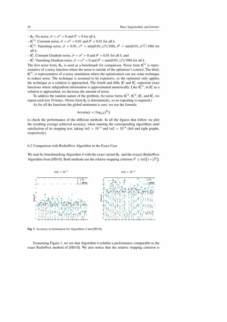
We start by benchmarking Algorithm 4 with the exact variant N0 and the (exact) RedistProxAlgorithm from [HS10]. Both methods use the relative stopping criterion δk ≤ tol

(1+ | f k |

).

tol = 10−3 tol = 10−6

Fig. 1 Accuracy at termination for Algorithms 4 and [HS10].

Examining Figure 1, we see that Algorithm 4 exhibits a performance comparable to theexact RedisProx method of [HS10]. We also notice that the relative stopping criterion is


fairly successful in reaching the desired accuracy (of 3 or 6 digits). When the tolerance is10−6, Algorithm 4 seems to behave somewhat better than RedistProx, possibly because theversion of the ηk-update employed in [HS10] is more likely to cause QP instabilities (recallRemark 1).

6.3 Impact of Noise on Solution Accuracy

Next, we explore convergence over the variety of error forms N f ,gc ,N f ,g

v ,Ngc ,Ng

v , taking as rela-tive stopping criterion δk ≤ max

(tol, σ

)(1+ | f k |

). (It is clearly unreasonable/not-meaningful

to aim for accuracy higher than the error bound.)

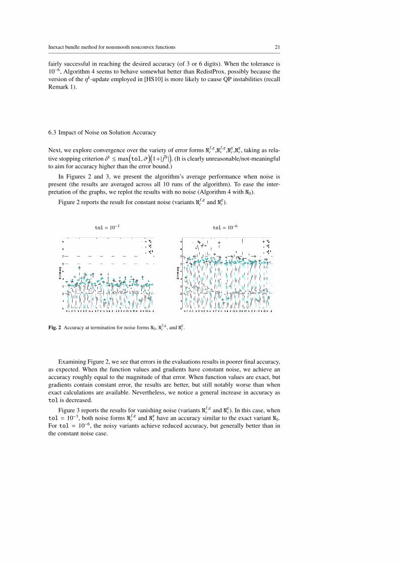
In Figures 2 and 3, we present the algorithm’s average performance when noise ispresent (the results are averaged across all 10 runs of the algorithm). To ease the inter-pretation of the graphs, we replot the results with no noise (Algorithm 4 with N0).

Figure 2 reports the result for constant noise (variants N f ,gc and Ng

c).

tol = 10−3 tol = 10−6

Fig. 2 Accuracy at termination for noise forms N0, N f ,gc , and Ng

c .

Examining Figure 2, we see that errors in the evaluations results in poorer final accuracy,as expected. When the function values and gradients have constant noise, we achieve anaccuracy roughly equal to the magnitude of that error. When function values are exact, butgradients contain constant error, the results are better, but still notably worse than whenexact calculations are available. Nevertheless, we notice a general increase in accuracy astol is decreased.

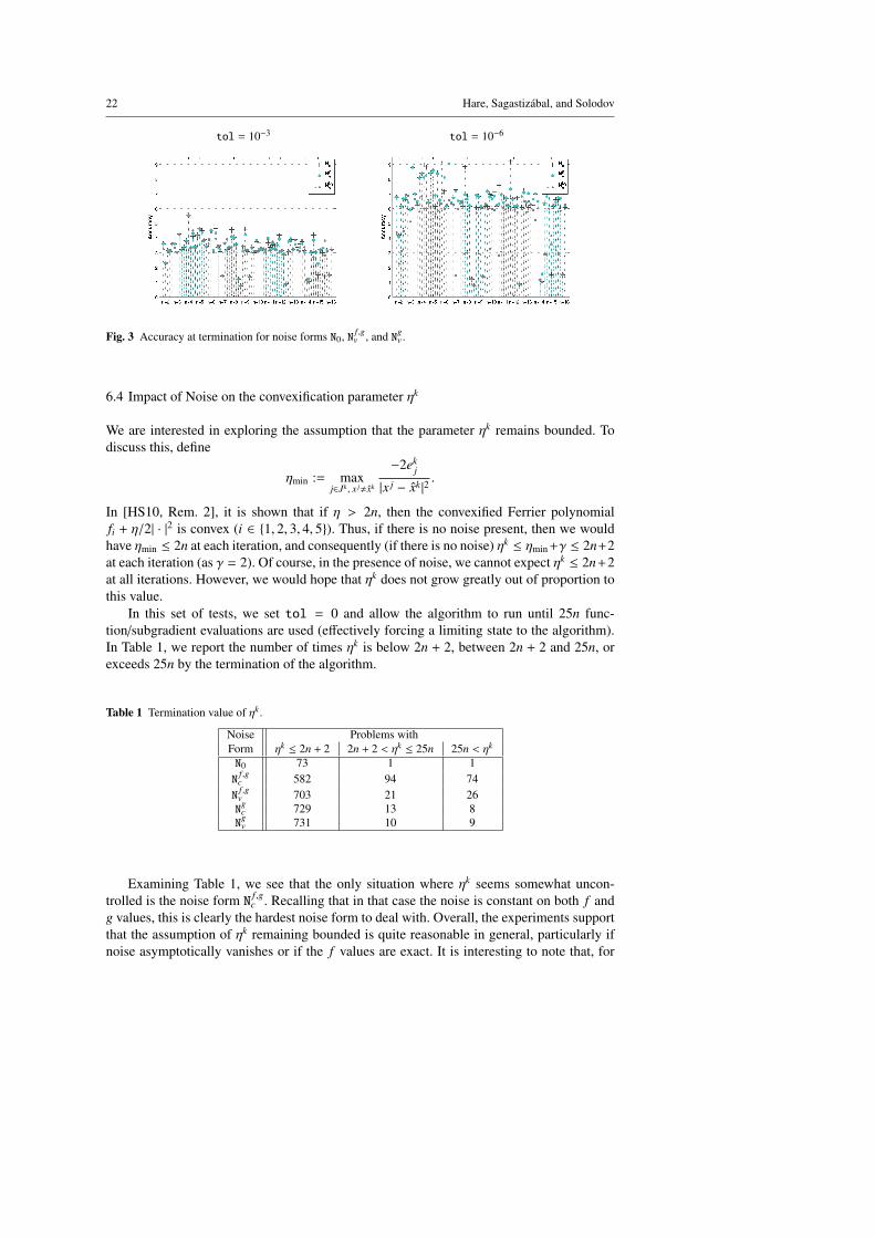
Figure 3 reports the results for vanishing noise (variants N f ,gv and Ng

v). In this case, whentol = 10−3, both noise forms N f ,g

v and Ngv have an accuracy similar to the exact variant N0.

For tol = 10−6, the noisy variants achieve reduced accuracy, but generally better than inthe constant noise case.


tol = 10−3 tol = 10−6

Fig. 3 Accuracy at termination for noise forms N0, N f ,gv , and Ng

v .

6.4 Impact of Noise on the convexification parameter ηk

We are interested in exploring the assumption that the parameter ηk remains bounded. Todiscuss this, define

ηmin := maxj∈Jk , x j,xk

−2ekj

|x j − xk |2.

In [HS10, Rem. 2], it is shown that if η > 2n, then the convexified Ferrier polynomialfi + η/2| · |2 is convex (i ∈ 1, 2, 3, 4, 5). Thus, if there is no noise present, then we wouldhave ηmin ≤ 2n at each iteration, and consequently (if there is no noise) ηk ≤ ηmin +γ ≤ 2n+2at each iteration (as γ = 2). Of course, in the presence of noise, we cannot expect ηk ≤ 2n+2at all iterations. However, we would hope that ηk does not grow greatly out of proportion tothis value.

In this set of tests, we set tol = 0 and allow the algorithm to run until 25n func-tion/subgradient evaluations are used (effectively forcing a limiting state to the algorithm).In Table 1, we report the number of times ηk is below 2n + 2, between 2n + 2 and 25n, orexceeds 25n by the termination of the algorithm.

Table 1 Termination value of ηk .

Noise Problems withForm ηk ≤ 2n + 2 2n + 2 < ηk ≤ 25n 25n < ηk

N0 73 1 1N

f ,gc 582 94 74N

f ,gv 703 21 26N

gc 729 13 8N

gv 731 10 9

Examining Table 1, we see that the only situation where ηk seems somewhat uncon-trolled is the noise form N f ,g

c . Recalling that in that case the noise is constant on both f andg values, this is clearly the hardest noise form to deal with. Overall, the experiments supportthat the assumption of ηk remaining bounded is quite reasonable in general, particularly ifnoise asymptotically vanishes or if the f values are exact. It is interesting to note that, for


all noise forms (including “no-noise”) and on all tests, Ferrier polynomial f4 in dimension14 results in ηk > 25n.

Acknowledgements The authors thank the referees for many useful and insightful comments. In fact, thisversion looks very much different from (and is much better than) the original, thanks to the input received.

References

[ANO09] P. Apkarian, D. Noll, and O. Prot. A proximity control algorithm to minimize nonsmooth andnonconvex semi-infinite maximum eigenvalue functions. J. Convex Anal., 16(3-4):641–666, 2009.

[AFGG11] A. Astorino, A. Frangioni, M. Gaudioso, and E. Gorgone. Piecewise-quadratic approximationsin convex numerical optimization. SIAM J. Optim., 21:1418–1438, 2011.

[BKS08] A. M. Bagirov, B. Karasozen, and M. Sezer. Discrete gradient method: derivative-free method fornonsmooth optimization. J. Optim. Theory Appl., 137(2):317–334, 2008.

[Bih85] Bihain. Optimization of upper semidifferentiable functions, J. Optim. Theory Appl., 44, 1985.[CSV09] A. R. Conn, K. Scheinberg, and L. N. Vicente. Introduction to Derivative-Free Optimization,

volume 8 of MPS/SIAM Book Series on Optimization. SIAM, 2009.[DG04] A. Daniilidis and P. Georgiev. Approximate convexity and submonotonicity. J. Math. Analysis

and Appl., 291(1): 292–301, 2004.[DSS09] A. Daniilidis, C. Sagastizabal, and M. Solodov. Identifying structure of nonsmooth convex func-

tions by the bundle technique. SIAM J. Optim., 20(2):820–840, 2009.[dAF09] G. d’Antonio and A. Frangioni. Convergence Analysis of Deflected Conditional Approximate

Subgradient Methods SIAM J. Optim., 20(1):357–386, 2009.[dOSL14] W. de Oliveira, C. Sagastizabal, and C. Lemarechal. Convex proximal bundle methods in depth:

a unified analysis for inexact oracles. Math. Program., 148(1-2):241–277, 2014.[ES10] G. Emiel and C. Sagastizabal. Incremental-like bundle methods with application to energy plan-

ning. Comp. Optim. Appl., 46:305–332, 2010.[Fer97] C. Ferrier, Bornes Duales de Problemes d’Optimisation Polynomiaux, Ph.D. thesis, Laboratoire

Approximation et Optimisation, Universite Paul Sabatier, Toulouse, France, 1997.[Fer00] C. Ferrier, Computation of the distance to semi-algebraic sets, ESAIM Control Optim. Calc.

Var., 5 (2000), pp. 139–156.[FLRS06] R. Fletcher, S. Leyffer, D. Ralph, and S. Scholtes. Local convergence of SQP methods for math-

ematical programs with equilibrium constraints. SIAM J. Optim., 17:259–286, 2006.[Gup77] A. M. Gupal. A method for the minimization of almost differentiable functions. Kibernetika

(Kiev), 1:114–116, 1977.[Hin01] M. Hintermuller. A proximal bundle method based on approximate subgradients. Comp. Optim.

Appl., 20:245–266, 2001.[HM12] W. Hare and M. Macklem. Derivative-free optimization methods for finite minimax problems.

Opt. Methods and Soft., 28(2): 300–312, 2013.[HN13] W. Hare and J. Nutini. A derivative-free approximate gradient sampling algorithm for finite min-

imax problems. Comput. Optim. Appl., 56(1):1–38, 2013.[HS10] W. Hare and C. Sagastizabal. A redistributed proximal bundle method for nonconvex optimiza-

tion. SIAM J. Optim., 20(5):2442–2473, 2010.[HUL93] J.-B. Hiriart-Urruty and C. Lemarechal. Convex analysis and minimization algorithms. II, volume

306 of Grundlehren der Mathematischen Wissenschaften [Fundamental Principles of Mathemat-ical Sciences]. Springer-Verlag, Berlin, 1993. Advanced theory and bundle methods.

[Kiw85a] K.C. Kiwiel. A linearization algorithm for nonsmooth minimization. Math. Oper. Res., 10(2):185–194, 1985.

[Kiw85b] K.C. Kiwiel. Methods of descent for nondifferentiable optimization. Springer-Verlag, Berlin,1985.

[Kiw95] K.C. Kiwiel. Approximations in proximal bundle methods and decomposition of convex pro-grams. J. Optim. Theory Appl., 84:529–548, 1995.

[Kiw96] K. C. Kiwiel. Restricted step and Levenberg-Marquardt techniques in proximal bundle methodsfor nonconvex nondifferentiable optimization. SIAM J. Optim., 6(1):227–249, 1996.

[Kiw04] K.C. Kiwiel. Convergence of Approximate and Incremental Subgradient Methods for ConvexOptimization SIAM J. Optim., 14(3):807–840, 2004.

[Kiw06] K.C. Kiwiel. A proximal bundle method with approximate subgradient linearizations. SIAM J.Optim., 16(4):1007–1023, 2006.


[Kiw10] K.C. Kiwiel. A nonderivative version of the gradient sampling algorithm for nonsmooth noncon-vex optimization. SIAM J. Optim., 20(4):1983–1994, 2010.

[Lem75] C. Lemarechal. An extension of Davidon methods to non differentiable problems. Math. Program.Study, 3:95–109, 1975. Nondifferentiable optimization.

[Lem78] C. Lemarechal. Bundle methods in nonsmooth optimization. In Nonsmooth optimization (Proc.IIASA Workshop, Laxenburg, 1977), volume 3 of IIASA Proc. Ser., pages 79–102. Pergamon,Oxford, 1978.

[Lem01] C. Lemarechal. Lagrangian relaxation. In Computational combinatorial optimization (SchloßDagstuhl, 2000), volume 2241 of Lecture Notes in Comput. Sci., pages 112–156. Springer, Berlin,2001.

[LSB81] C. Lemarechal, J.-J. Strodiot, and A. Bihain. On a bundle algorithm for nonsmooth optimization.In Nonlinear programming, 4 (Madison, Wis., 1980), pages 245–282. Academic Press, New York,1981.

[LV98] L. Luksan and J. Vlcek. A bundle-Newton method for nonsmooth unconstrained minimization.Math. Program., 83(3, Ser. A):373–391, 1998.

[LV01] L. Luksan and J. Vlcek. Globally Convergent Variable Metric Method for Nonconvex Nondiffer-entiable Unconstrained Minimization. J. Optim. Theory Appl., 151(3):425–454, 2011.

[LS05] C. J. Luz and A. Schrijver. A Convex Quadratic Characterization of the Lovasz Theta Number.SIAM J. Discrete Math., 19(2):382–387, 2005.

[Mif77] R. Mifflin. Semismooth and semiconvex functions in constrained optimization. SIAM J. ControlOptim., 15(6):959–972, 1977.

[Mif82a] R. Mifflin. Convergence of a modification of Lemarechal’s algorithm for nonsmooth optimization.In Progress in nondifferentiable optimization, volume 8 of IIASA Collaborative Proc. Ser. CP-82,pages 85–95. Internat. Inst. Appl. Systems Anal., Laxenburg, 1982.

[Mif82b] R. Mifflin. A modification and extension of Lemarechal’s algorithm for nonsmooth minimization.Math. Program. Study, 17:77–90, 1982. Nondifferential and variational techniques in optimization(Lexington, Ky., 1980).

[MN92] M. M. Makela and P. Neittaanmaki. Nonsmooth optimization. World Scientific Publishing Co.Inc., River Edge, NJ, 1992. Analysis and algorithms with applications to optimal control.

[NB10] A. Nedic and D. P. Bertsekas. The effect of deterministic noise in subgradient methods. Math.Program., 125:75–99, 2010.

[Nol13] D. Noll. Bundle method for non-convex minimization with inexact subgradients and functionvalues. In Computational and Analytical Mathematics, Vol. 50, 2013, pp. 555 - 592. SpringerProceedings in Mathematics.

[PT06] M. Pinar, and M. Teboulle. On Semidefinite Bounds for Maximization of a Non-convex QuadraticObjective over the L1-Unit Ball. RAIRO Oper. Research 40(3):253–265, 2006.

[Pol87] B.T. Polyak. Introduction to Optimization. Optimization Software, Inc., Publications Division,New York, 1987.

[RC04] C. P. Robert and G. Casella. Monte Carlo statistical methods. Springer Texts in Statistics.Springer-Verlag, New York, second edition, 2004.

[RW98] R. T. Rockafellar and J. J.-B. Wets. Variational analysis, volume 317 of Grundlehren der Mathe-matischen Wissenschaften [Fundamental Principles of Mathematical Sciences]. Springer-Verlag,Berlin, 1998.

[Sag12] C. Sagastizabal. Divide to conquer: decomposition methods for energy optimization. Math.Program. B, 134(1):187–222, 2012.

[SS05] C. Sagastizabal and M. Solodov. An infeasible bundle method for nonsmooth convex constrainedoptimization without a penalty function or a filter. SIAM J. Optim., 16:146–169, 2005.

[Sol03] M. V. Solodov. On approximations with finite precision in bundle methods for nonsmooth opti-mization. J. Optim. Theory Appl., 119:151–165, 2003.

[Sol10] M. V. Solodov. Constraint qualifications. In Wiley Encyclopedia of Operations Research andManagement Science, James J. Cochran, et al. (editors), John Wiley & Sons, Inc., 2010.

[SZ98] M. V. Solodov and S. K. Zavriev. Error stabilty properties of generalized gradient-type algorithms.J. Optim. Theory Appl., 98:663–680, 1998.

[SP81] J.E. Spingarn. Submonotone subdifferentials of Lipschitz functions. Trans. Amer. Math. Soc.,264:77–89, 1981.

Documents

A proximal bundle method for nonsmooth nonconvex functions