A quadratic plane triangular element immune to quadratic mesh distortions under quadratic displacement fields

Comput. Methods Appl. Mech. Engrg. 195 (2006) 1207–1223

www.elsevier.com/locate/cma

A quadratic plane triangular element immune to quadraticmesh distortions under quadratic displacement fields

K.M. Liew a,b, S. Rajendran b,*, J. Wang a,b

a Nanyang Centre for Supercomputing and Visualisation, Nanyang Technological University,

Nanyang Avenue, Singapore 639798, Singaporeb School of Mechanical and Aerospace Engineering, Centre for Advanced Numerical Engineering Simulations,

Nanyang Technological University, 50 Nanyang Avenue, Singapore 639798, Singapore

Accepted 25 April 2005

Abstract

A quadratic plane triangular element is developed extending the concepts of US-QUAD8 element. The element

belongs to the broad class of Petrov–Galerkin formulation which is characterized by the choice of test and trial func-

tions from different spaces. The performance of the proposed element has been studied for typical static and free vibra-

tion problems. The element exhibits a high degree of tolerance to mesh distortions as compared to the classical

isoparametric quadratic triangular element. For undistorted meshes, however, the performance is similar to that of

the classical element.

� 2005 Elsevier B.V. All rights reserved.

Keywords: Mesh distortion; Quadratic triangular element; 6-node triangular element; US-TRIA6; Distortion tolerant; Distortion

immune

1. Introduction

The classical isoparametric 6-noded quadratic plane triangular element is one of the successful elements

for plane elasticity problems. The element can ensure displacement compatibility for all admissible geo-

metries. However, the quadratic completeness of the displacement interpolation, which is necessary to guar-

antee reproducibility of the second order Cartesian monomial terms, is not satisfied for all admissible

element geometries.

0045-7825/$ - see front matter � 2005 Elsevier B.V. All rights reserved.

doi:10.1016/j.cma.2005.04.012

* Corresponding author. Tel.: +65 6790 5865; fax: +65 6791 1859.

E-mail address: [email protected] (S. Rajendran).

mailto:[email protected]

1208 K.M. Liew et al. / Comput. Methods Appl. Mech. Engrg. 195 (2006) 1207–1223

As an alternative to the above element, one can formulate a 6-node plane triangular element using non-

parametric shape functions, i.e., functions written in terms of the global Cartesian coordinates. Such an ele-

ment does satisfy all the quadratic completeness requirements for all admissible element geometries.

Nevertheless, it does not satisfy compatibility requirements for all admissible geometries, and hence is

not popular.The quadratic triangular element was introduced by de Veubeke in mid sixties [1]. Although this element

is widely used, the accuracy of computed results deteriorates when the element geometry is distorted. A

common approach to deal with mesh distortion problem adopted by the commercial FE software is to iden-

tify the badly shaped elements using some distortion metric [2–6] and use mesh enhancing techniques [7–9]

to improve the shape of such elements. In the paper, we investigate a quadratic element that shows immu-

nity to mesh distortion under quadratic displacement fields.

The unsymmetric quadrilateral element (US-QUAD8) developed by Rajendran and Liew [10] uses para-

metric shape functions and metric shape functions as test and trial functions, respectively. US-QUAD8gives the best performance under distorted meshes as compared to its peer elements like QUAD8. Further

investigations into US-QUAD8 element and extension of the formulation to 20-node solid hexahedron ele-

ment confirm the high degree of distortion tolerance of unsymmetric formulation [11,12]. In this paper, the

unsymmetric formulation is extended to the quadratic plane triangular element. For ease of reference, the

proposed element is hereinafter called the unsymmetric 6-node triangular element (US-TRIA6).

The distortion sensitivity studies on triangular elements are scarce as compared to those on quadrilateral

elements. Lee and Bathe [13] investigated the distortion sensitivity of the 8-node and 9-node isoparametric

quadrilateral elements and attributed it to the absence of certain monomial terms in the shape functions.Lautersztajn and Samuelsson [14] observed that the quadrilateral element Q6 of Wilson et al. [15] and

QM6 of Taylor et al. [16] can be rendered ‘‘insensitive’’ to a particular type of mesh distortion by increasing

the order of the interpolation functions. The hybrid stress element of Pian and Sumihara [17] and the en-

hanced assumed strain (EAS) element of Simo and Rifai [18] exhibit good performance in general but poor

performance in the presence of mesh distortions. Yeo and Lee [19] and Sze [20] improved the performance

of the 5b element of Pian and Sumihara [17] under trapezoidal meshes. Korelc and Wriggers [21] improved

the EAS element by expanding the shape functions as a Taylor�s series expansion while Cao et al. [22] used a

penalty approach. The hybrid-Trefftz elements [23,24], non-conforming elements with drilling degrees offreedom proposed by Choi et al. [25], and quadrilateral area coordinate elements [26] are some of the recent

efforts in enhancing the performance of quadrilateral elements under distorted meshes.

2. Metric and parametric shape functions

A quadratic triangular element has 6-nodes, and hence ideally we want the element to reproduce exactly

a complete quadratic Cartesian polynomial of the form

u ¼uðx; yÞvðx; yÞ

� �¼ a1 þ a2xþ a3y þ a4x2 þ a5xy þ a6y2

b1 þ b2xþ b3y þ b4x2 þ b5xy þ b6y2

� �; ð1Þ

where ai and bi (i = 1,2, . . ., 6) are arbitrary constants. In terms of the metric shape functions, Mi � Mi(x,y)

which are yet to be derived, the finite element approximation of the displacement field is written as

uðeÞðx; yÞ ¼X6

i¼1

MiuðeÞi ; vðeÞðx; yÞ ¼

X6

i¼1

MivðeÞi ; ð2; 3Þ

where uðeÞi and vðeÞi are the finite element nodal displacements corresponding to ith node, and the superscript

(e) signifies the element level interpolation. The shape functions, Mi, may also be looked up on as functions

K.M. Liew et al. / Comput. Methods Appl. Mech. Engrg. 195 (2006) 1207–1223 1209

of natural coordinates, (n,g), by using the usual isoparametric mapping, (x,y) ! (n,g). For the element to

reproduce the quadratic field (1), the shape functions chosen should satisfy the condition

uðx; yÞ ¼ uðeÞðx; yÞ and vðx; yÞ ¼ vðeÞðx; yÞ. ð4; 5Þ
Using Eqs. (1)–(3) in the above equation, we can show that the shape functions must satisfy the follow-
ing conditions [27]:
X6
i¼1

Mixpi y

qi ¼ xpyq; p; q ¼ 0; 1; 2 and 0 6 ðp þ qÞ 6 2; ð6Þ

where xpyq is a typical monomial term in Eq. (1). The metric shape functions can be directly obtained by

solving the above system of six simultaneous equations which, in matrix form, becomes

PU ¼ pðx; yÞ; ð7Þ
where
U ¼ ½M1;M2;M3; . . . ;M6�T; ð8Þ

pðx; yÞ ¼ ½1; x; y; x2; xy; y2�T ð9Þ
and
P ¼

1 x1 y1 x21 x1y1 y211 x2 y2 x22 x2y2 y221 x3 y3 x23 x3y3 y23

..

. ... ..

. ... ..

. ...

1 x6 y6 x26 x6y6 y26

2666666664

3777777775

T

. ð10Þ

The metric shape functions can be obtained by solving Eq. (7) as

U ¼ P�1pðx; yÞ. ð11Þ
The corresponding shape function matrix (for use in Section 3) is defined as
M ¼M1 0 M2 � � � M6 0

0 M1 0 M2 � � � M6

� �. ð12Þ

Although all the completeness requirements (Eq. (6)) are inherently satisfied by the metric shape func-

tions, the inter-element displacement continuity along all the three edges of the element are satisfied only

for limited element geometries like right-angled triangle. For distorted element geometries, the inter-ele-

ment displacement continuity is not in general guaranteed.

The parametric shape functions widely used in the classical isoparametric formulation, on the contrary,

satisfy inter-element displacement continuity for all (admissible) geometries. The corresponding shape func-

tion matrix (for use in Section 3) is defined as

N ¼N 1 0 N 2 � � � N 6 0

0 N 1 0 N 2 � � � N 6

� �; ð13Þ

N 1 ¼ nð2n� 1Þ; N 2 ¼ gð2g� 1Þ; N 3 ¼ fð2f� 1Þ; ð14; 15; 16Þ

N 4 ¼ 4ng; N 5 ¼ 4fg; N 6 ¼ 4nf; ð16; 17; 18Þ

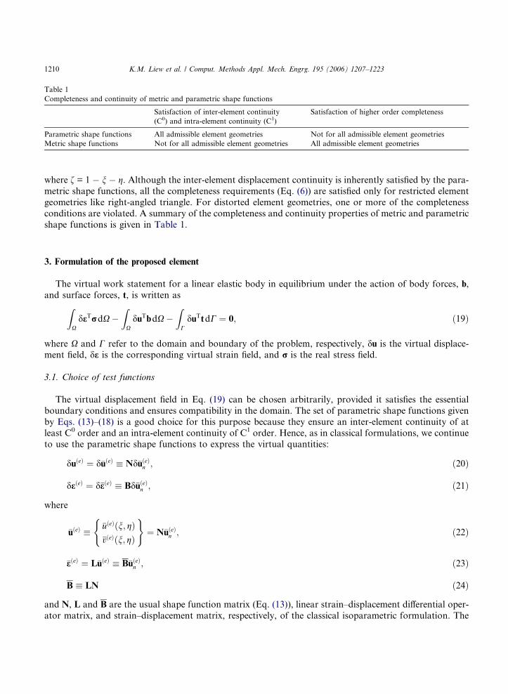
Table 1

Completeness and continuity of metric and parametric shape functions

Satisfaction of inter-element continuity

(C0) and intra-element continuity (C1)

Satisfaction of higher order completeness

Parametric shape functions All admissible element geometries Not for all admissible element geometries

Metric shape functions Not for all admissible element geometries All admissible element geometries


where f = 1 � n � g. Although the inter-element displacement continuity is inherently satisfied by the para-

metric shape functions, all the completeness requirements (Eq. (6)) are satisfied only for restricted element

geometries like right-angled triangle. For distorted element geometries, one or more of the completeness

conditions are violated. A summary of the completeness and continuity properties of metric and parametric

shape functions is given in Table 1.

3. Formulation of the proposed element

The virtual work statement for a linear elastic body in equilibrium under the action of body forces, b,

and surface forces, t, is written as
ZXdeTrdX�
ZXduTbdX�

ZCduTtdC ¼ 0; ð19Þ

where X and C refer to the domain and boundary of the problem, respectively, du is the virtual displace-ment field, de is the corresponding virtual strain field, and r is the real stress field.

3.1. Choice of test functions

The virtual displacement field in Eq. (19) can be chosen arbitrarily, provided it satisfies the essential

boundary conditions and ensures compatibility in the domain. The set of parametric shape functions given

by Eqs. (13)–(18) is a good choice for this purpose because they ensure an inter-element continuity of at

least C0 order and an intra-element continuity of C1 order. Hence, as in classical formulations, we continueto use the parametric shape functions to express the virtual quantities:

duðeÞ ¼ d�uðeÞ � Nd�uðeÞn ; ð20Þ

deðeÞ ¼ d�eðeÞ � Bd�uðeÞn ; ð21Þ

where

�uðeÞ � �uðeÞðn; gÞ�vðeÞðn; gÞ

( )¼ N�uðeÞn ; ð22Þ

�eðeÞ ¼ L�uðeÞ � B�uðeÞn ; ð23Þ

B � LN ð24Þ

and N, L and B are the usual shape function matrix (Eq. (13)), linear strain–displacement differential oper-

ator matrix, and strain–displacement matrix, respectively, of the classical isoparametric formulation. The


over-score in some of the quantities in Eqs. (20)–(24) signifies the choice of parametric shape functions to

express the virtual quantities and subscript �n� refers to nodal quantities.

3.2. Choice of trial functions

In the classical isoparametric formulation, the trial solution is also interpolated using the same paramet-

ric shape functions as for test functions, in which case, the nodal forces due to error stress field can be

expressed as

�fðeÞerror ¼

ZXðeÞ

BTð�rðeÞ � rðeÞÞdXðeÞ. ð25Þ

These error nodal forces are responsible for the poor performance of the classical element under mesh dis-

tortion. In the proposed unsymmetric formulation, we aim to reduce the error nodal forces to zero for

problems where the exact solution is utmost a quadratic displacement field of the form (1). This is achieved

by using a metric interpolation for trial solution

uðeÞ � uðeÞðx; yÞvðeÞðx; yÞ

( )¼ MuðeÞn ; ð26Þ

eðeÞ ¼ LuðeÞ � bBuðeÞn ; ð27Þ

bB � LM; ð28Þ

rðeÞ ¼ DeðeÞ; ð29Þ

whereM is the metric shape function matrix as defined in Eq. (12). The nodal forces due to stress error field

are then expressed as

fðeÞerror ¼

ZXðeÞ

bBTðrðeÞ � rðeÞÞdXðeÞ. ð30Þ

Using Eqs. (26)–(29), we realize that the error nodal forces given by Eq. (30) reduces to zero, i.e.,

fðeÞerror ¼

ZXðeÞ

bBTDLðuðeÞðx; yÞ � uðeÞðx; yÞÞdXðeÞ ¼ 0; ð31Þ

for all problems involving quadratic exact displacement field. This is because the metric shape functions

render the quantity within the brackets in Eq. (31) to zero, i.e., ðuðeÞðx; yÞ � uðeÞðx; yÞÞ ¼ 0 by virtue of

the fact that the very same condition (viz., Eqs. (4) and (5)) are used to derive metric shape functions. Thus,

these element integrals vanish irrespective of the element geometry, distorted or undistorted, as long as the

order of the exact polynomial displacement field is quadratic or less. Thus, the metric shape functions offera better choice than their parametric counterpart for the interpolation of trial solution.

For the implementation of the proposed element, explicit analytical expressions of metric shape func-

tions are not needed. Numerical values of these shape functions can be obtained by solving Eq. (11).

The derivative values of metric shape functions that are needed to construct the bB matrix at the quadrature

points are simply obtained as, U,x = P�1p,x and U,y = P�1p,y, which are the derivative versions of Eq. (11).

The P�1 matrix appearing in these equations as well as Eq. (11) needs to be evaluated just once per element

irrespective of the number of Gauss points. Note that we cannot rule out the theoretical possibility of P

matrix becoming singular for certain nodal configurations. For the geometrical shapes considered in thispaper, such a problem has not been encountered.

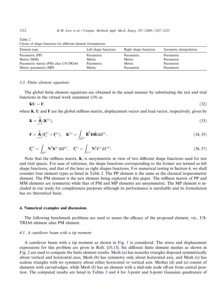
Table 2

Choice of shape functions for different element formulations

Element type Left shape functions Right shape functions Geometry interpolation

Parametric (PP) Parametric Parametric Parametric

Metric (MM) Metric Metric Parametric

Parametric–metric (PM) alias US-TRIA6 Parametric Metric Parametric

Metric–parametric (MP) Metric Parametric Parametric


3.3. Finite element equations

The global finite element equations are obtained in the usual manner by substituting the test and trial

functions in the virtual work statement (19) as

KU ¼ F; ð32Þ
where K, U and F are the global stiffness matrix, displacement vector and load vector, respectively, given by
K ¼ AN

e¼1ðKðeÞÞ; ð33Þ

F ¼ AN

e¼1ðfðeÞb þ fðeÞt Þ; KðeÞ ¼

ZXðeÞ

BTDbB dXðeÞ; ð34; 35Þ

fðeÞb ¼

ZXðeÞ

NTbðeÞ dXðeÞ; fðeÞt ¼ZCðeÞ

NTtðeÞ dCðeÞ. ð36; 37Þ

Note that the stiffness matrix, K, is unsymmetric in view of two different shape functions used for test

and trial spaces. For ease of reference, the shape functions corresponding to the former are termed as left

shape functions, and that of the later as right shapes functions. For numerical testing in Section 4, we shall

consider four element types as listed in Table 2. The PP element is the same as the classical isoparametricelement. The PM element is the new element being explored in this paper. The stiffness matrix of PP and

MM elements are symmetric while that of PM and MP elements are unsymmetric. The MP element is in-

cluded in our study for completeness purposes although its performance is unreliable and its formulation

has no theoretical basis.

4. Numerical examples and discussions

The following benchmark problems are used to assess the efficacy of the proposed element, viz., US-

TRIA6 element alias PM element.

4.1. A cantilever beam with a tip moment

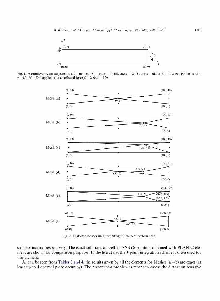
A cantilever beam with a tip moment as shown in Fig. 1 is considered. The stress and displacement

expressions for this problem are given in Refs. [10,13]. Six different finite element meshes as shown in

Fig. 2 are used to compute the finite element results. Mesh (a) has isosceles triangles disposed symmetricallyabout vertical and horizontal axes, Mesh (b) has symmetry only about horizontal axis, and Mesh (c) has

scalene triangles with no symmetry about either horizontal or vertical axis. Meshes (d) and (e) consist of

elements with curved-edges, while Mesh (f) has an element with a mid-side node off-set from central posi-

tion. The computed results are listed in Tables 3 and 4 for 3-point and 6-point Gaussian quadrature of

y

x

M

(0, 0)

(0, c)

(L, 0)

(L, c)

Fig. 1. A cantilever beam subjected to a tip moment. L = 100, c = 10, thickness = 1.0, Young�s modulus E = 1.0 · 107, Poisson�s ratiom = 0.3, M = 20c2 applied as a distributed force fx = 240y/c � 120.

Mesh (a)

(0, 10)

(0, 0)

(100, 10)

(100, 0)

(50, 5)

Mesh (b)

(0, 10) (100, 10)

(100, 0)(0, 0)

(75, 5)

Mesh (c)

(0, 10)

(0, 0)

(75, 7.5)

(100, 0)

(100, 10)

Mesh (d)

(0, 10)

(0, 0)

(100, 10)

(100, 0)

(50, 5)

Mesh (e)

(0, 10)

(0, 0) (100, 0)

(100, 10)

(75, 5)

Mesh (f)

(0, 10)

(0, 0) (100, 0)

(100, 10)

(50, 5)

(65, 3.5)

(75, 5.1)

(87.5, 8.5)(87.5, 1.5)

Fig. 2. Distorted meshes used for testing the element performance.


stiffness matrix, respectively. The exact solutions as well as ANSYS solution obtained with PLANE2 ele-

ment are shown for comparison purposes. In the literature, the 3-point integration scheme is often used for

this element.As can be seen from Tables 3 and 4, the results given by all the elements for Meshes (a)–(c) are exact (at

least up to 4 decimal place accuracy). The present test problem is meant to assess the distortion sensitive

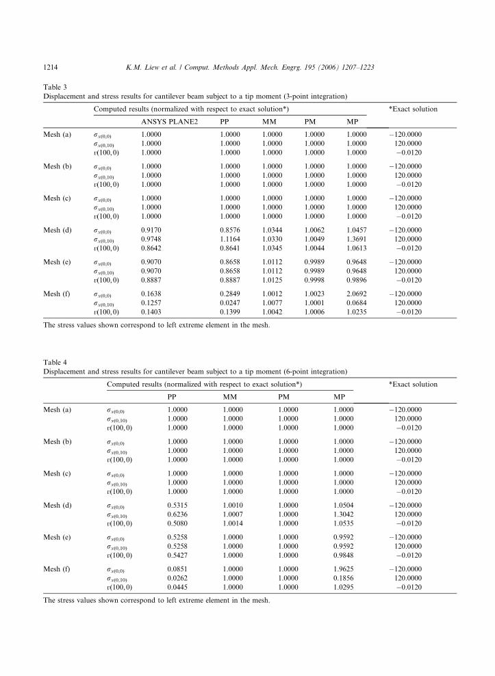
Table 3

Displacement and stress results for cantilever beam subject to a tip moment (3-point integration)

Computed results (normalized with respect to exact solution*) *Exact solution

ANSYS PLANE2 PP MM PM MP

Mesh (a) rx(0,0) 1.0000 1.0000 1.0000 1.0000 1.0000 �120.0000

rx(0,10) 1.0000 1.0000 1.0000 1.0000 1.0000 120.0000

v(100,0) 1.0000 1.0000 1.0000 1.0000 1.0000 �0.0120

Mesh (b) rx(0,0) 1.0000 1.0000 1.0000 1.0000 1.0000 �120.0000

rx(0,10) 1.0000 1.0000 1.0000 1.0000 1.0000 120.0000

v(100,0) 1.0000 1.0000 1.0000 1.0000 1.0000 �0.0120

Mesh (c) rx(0,0) 1.0000 1.0000 1.0000 1.0000 1.0000 �120.0000

rx(0,10) 1.0000 1.0000 1.0000 1.0000 1.0000 120.0000

v(100,0) 1.0000 1.0000 1.0000 1.0000 1.0000 �0.0120

Mesh (d) rx(0,0) 0.9170 0.8576 1.0344 1.0062 1.0457 �120.0000

rx(0,10) 0.9748 1.1164 1.0330 1.0049 1.3691 120.0000

v(100,0) 0.8642 0.8641 1.0345 1.0044 1.0613 �0.0120

Mesh (e) rx(0,0) 0.9070 0.8658 1.0112 0.9989 0.9648 �120.0000

rx(0,10) 0.9070 0.8658 1.0112 0.9989 0.9648 120.0000

v(100,0) 0.8887 0.8887 1.0125 0.9998 0.9896 �0.0120

Mesh (f) rx(0,0) 0.1638 0.2849 1.0012 1.0023 2.0692 �120.0000

rx(0,10) 0.1257 0.0247 1.0077 1.0001 0.0684 120.0000

v(100,0) 0.1403 0.1399 1.0042 1.0006 1.0235 �0.0120

The stress values shown correspond to left extreme element in the mesh.

Table 4

Displacement and stress results for cantilever beam subject to a tip moment (6-point integration)


PP MM PM MP

Mesh (a) rx(0,0) 1.0000 1.0000 1.0000 1.0000 �120.0000

rx(0,10) 1.0000 1.0000 1.0000 1.0000 120.0000

v(100,0) 1.0000 1.0000 1.0000 1.0000 �0.0120

Mesh (b) rx(0,0) 1.0000 1.0000 1.0000 1.0000 �120.0000

rx(0,10) 1.0000 1.0000 1.0000 1.0000 120.0000

v(100,0) 1.0000 1.0000 1.0000 1.0000 �0.0120

Mesh (c) rx(0,0) 1.0000 1.0000 1.0000 1.0000 �120.0000

rx(0,10) 1.0000 1.0000 1.0000 1.0000 120.0000

v(100,0) 1.0000 1.0000 1.0000 1.0000 �0.0120

Mesh (d) rx(0,0) 0.5315 1.0010 1.0000 1.0504 �120.0000

rx(0,10) 0.6236 1.0007 1.0000 1.3042 120.0000

v(100,0) 0.5080 1.0014 1.0000 1.0535 �0.0120

Mesh (e) rx(0,0) 0.5258 1.0000 1.0000 0.9592 �120.0000

rx(0,10) 0.5258 1.0000 1.0000 0.9592 120.0000

v(100,0) 0.5427 1.0000 1.0000 0.9848 �0.0120

Mesh (f) rx(0,0) 0.0851 1.0000 1.0000 1.9625 �120.0000

rx(0,10) 0.0262 1.0000 1.0000 0.1856 120.0000

v(100,0) 0.0445 1.0000 1.0000 1.0295 �0.0120



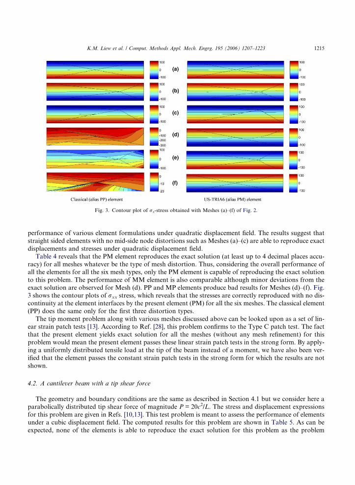
Fig. 3. Contour plot of rx-stress obtained with Meshes (a)–(f) of Fig. 2.


performance of various element formulations under quadratic displacement field. The results suggest that

straight sided elements with no mid-side node distortions such as Meshes (a)–(c) are able to reproduce exact

displacements and stresses under quadratic displacement field.

Table 4 reveals that the PM element reproduces the exact solution (at least up to 4 decimal places accu-racy) for all meshes whatever be the type of mesh distortion. Thus, considering the overall performance of

all the elements for all the six mesh types, only the PM element is capable of reproducing the exact solution

to this problem. The performance of MM element is also comparable although minor deviations from the

exact solution are observed for Mesh (d). PP and MP elements produce bad results for Meshes (d)–(f). Fig.

3 shows the contour plots of rxx stress, which reveals that the stresses are correctly reproduced with no dis-

continuity at the element interfaces by the present element (PM) for all the six meshes. The classical element

(PP) does the same only for the first three distortion types.

The tip moment problem along with various meshes discussed above can be looked upon as a set of lin-ear strain patch tests [13]. According to Ref. [28], this problem confirms to the Type C patch test. The fact

that the present element yields exact solution for all the meshes (without any mesh refinement) for this

problem would mean the present element passes these linear strain patch tests in the strong form. By apply-

ing a uniformly distributed tensile load at the tip of the beam instead of a moment, we have also been ver-

ified that the element passes the constant strain patch tests in the strong form for which the results are not

shown.

4.2. A cantilever beam with a tip shear force

The geometry and boundary conditions are the same as described in Section 4.1 but we consider here a

parabolically distributed tip shear force of magnitude P = 20c2/L. The stress and displacement expressions

for this problem are given in Refs. [10,13]. This test problem is meant to assess the performance of elements

under a cubic displacement field. The computed results for this problem are shown in Table 5. As can be

expected, none of the elements is able to reproduce the exact solution for this problem as the problem

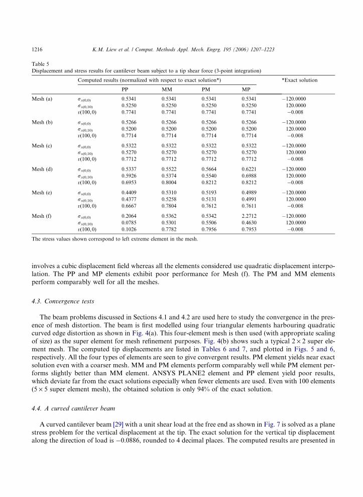
Table 5

Displacement and stress results for cantilever beam subject to a tip shear force (3-point integration)


PP MM PM MP

Mesh (a) rx(0,0) 0.5341 0.5341 0.5341 0.5341 �120.0000

rx(0,10) 0.5250 0.5250 0.5250 0.5250 120.0000

v(100,0) 0.7741 0.7741 0.7741 0.7741 �0.008

Mesh (b) rx(0,0) 0.5266 0.5266 0.5266 0.5266 �120.0000

rx(0,10) 0.5200 0.5200 0.5200 0.5200 120.0000

v(100,0) 0.7714 0.7714 0.7714 0.7714 �0.008

Mesh (c) rx(0,0) 0.5322 0.5322 0.5322 0.5322 �120.0000

rx(0,10) 0.5270 0.5270 0.5270 0.5270 120.0000

v(100,0) 0.7712 0.7712 0.7712 0.7712 �0.008

Mesh (d) rx(0,0) 0.5337 0.5522 0.5664 0.6221 �120.0000

rx(0,10) 0.5926 0.5374 0.5540 0.6988 120.0000

v(100,0) 0.6953 0.8004 0.8212 0.8212 �0.008

Mesh (e) rx(0,0) 0.4409 0.5310 0.5193 0.4989 �120.0000

rx(0,10) 0.4377 0.5258 0.5131 0.4991 120.0000

v(100,0) 0.6667 0.7804 0.7612 0.7611 �0.008

Mesh (f) rx(0,0) 0.2064 0.5362 0.5342 2.2712 �120.0000

rx(0,10) 0.0785 0.5301 0.5506 0.4630 120.0000

v(100,0) 0.1026 0.7782 0.7956 0.7953 �0.008



involves a cubic displacement field whereas all the elements considered use quadratic displacement interpo-

lation. The PP and MP elements exhibit poor performance for Mesh (f). The PM and MM elements

perform comparably well for all the meshes.

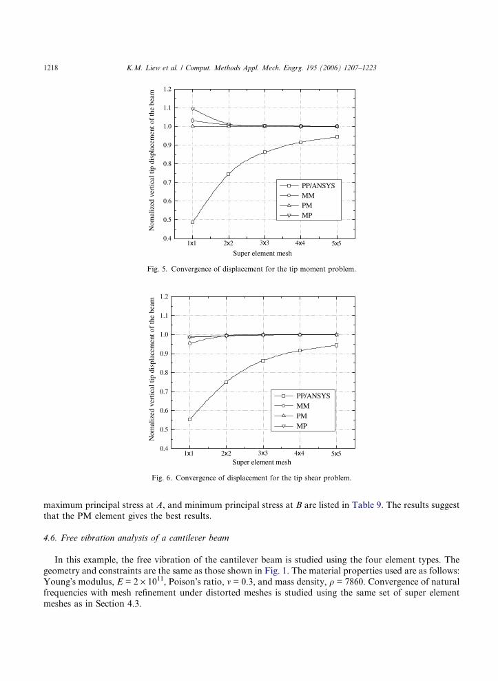
4.3. Convergence tests

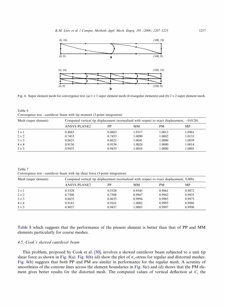
The beam problems discussed in Sections 4.1 and 4.2 are used here to study the convergence in the pres-

ence of mesh distortion. The beam is first modelled using four triangular elements harbouring quadraticcurved edge distortion as shown in Fig. 4(a). This four-element mesh is then used (with appropriate scaling

of size) as the super element for mesh refinement purposes. Fig. 4(b) shows such a typical 2 · 2 super ele-

ment mesh. The computed tip displacements are listed in Tables 6 and 7, and plotted in Figs. 5 and 6,

respectively. All the four types of elements are seen to give convergent results. PM element yields near exact

solution even with a coarser mesh. MM and PM elements perform comparably well while PM element per-

forms slightly better than MM element. ANSYS PLANE2 element and PP element yield poor results,

which deviate far from the exact solutions especially when fewer elements are used. Even with 100 elements

(5 · 5 super element mesh), the obtained solution is only 94% of the exact solution.

4.4. A curved cantilever beam

A curved cantilever beam [29] with a unit shear load at the free end as shown in Fig. 7 is solved as a plane

stress problem for the vertical displacement at the tip. The exact solution for the vertical tip displacement

along the direction of load is �0.0886, rounded to 4 decimal places. The computed results are presented in

(0, 10)

(0, 0)

(100, 10)

(100, 0)a

(0, 10)

(0, 0) (100, 0)

(100, 10)

b

Fig. 4. Super element mesh for convergence test. (a) 1 · 1 super element mesh (4 triangular elements) and (b) 2 · 2 super element mesh.

Table 6

Convergence test—cantilever beam with tip moment (3-point integration)

Mesh (super element) Computed vertical tip displacement (normalized with respect to exact displacement, �0.0120)


1 · 1 0.4863 0.4863 1.0317 1.0013 1.0961

2 · 2 0.7453 0.7453 1.0090 1.0002 1.0133

3 · 3 0.8621 0.8621 1.0041 1.0000 1.0039

4 · 4 0.9156 0.9156 1.0024 1.0000 1.0014

5 · 5 0.9435 0.9435 1.0016 1.0000 1.0005

Table 7

Convergence test—cantilever beam with tip shear force (3-point integration)

Mesh (super element) Computed vertical tip displacement (normalized with respect to exact displacement, 0.008)


1 · 1 0.5528 0.5528 0.9545 0.9861 0.9872

2 · 2 0.7508 0.7508 0.9947 0.9942 0.9935

3 · 3 0.8635 0.8635 0.9994 0.9985 0.9975

4 · 4 0.9161 0.9161 1.0002 0.9995 0.9986

5 · 5 0.9437 0.9437 1.0003 0.9997 0.9990


Table 8 which suggests that the performance of the present element is better than that of PP and MM

elements particularly for coarse meshes.

4.5. Cook’s skewed cantilever beam

This problem, proposed by Cook et al. [30], involves a skewed cantilever beam subjected to a unit tip

shear force as shown in Fig. 8(a). Fig. 8(b)–(d) show the plot of rx-stress for regular and distorted meshes.

Fig. 8(b) suggests that both PP and PM are similar in performance for the regular mesh. A scrutiny of

smoothness of the contour lines across the element boundaries in Fig. 8(c) and (d) shows that the PM ele-

ment gives better results for the distorted mesh. The computed values of vertical deflection at C, the

0.4

0.5

0.6

0.7

0.8

0.9

1.0

1.1

1.2

5x54x43x32x21x1

Nom

aliz

ed v

ertic

al ti

p di

spla

cem

ent o

f th

e be

am

Super element mesh

PP/ANSYSMMPMMP

Fig. 5. Convergence of displacement for the tip moment problem.

0.4

0.5

0.6

0.7

0.8

0.9

1.0

1.1

1.2

5x54x43x32x21x1

Nom

aliz

ed v

ertic

al ti

p di

spla

cem

ent o

f th

e be

am

Super element mesh

PP/ANSYS MM PM MP

Fig. 6. Convergence of displacement for the tip shear problem.


maximum principal stress at A, and minimum principal stress at B are listed in Table 9. The results suggest

that the PM element gives the best results.

4.6. Free vibration analysis of a cantilever beam

In this example, the free vibration of the cantilever beam is studied using the four element types. The

geometry and constraints are the same as those shown in Fig. 1. The material properties used are as follows:

Young�s modulus, E = 2 · 1011, Poison�s ratio, m = 0.3, and mass density, q = 7860. Convergence of naturalfrequencies with mesh refinement under distorted meshes is studied using the same set of super element

meshes as in Section 4.3.

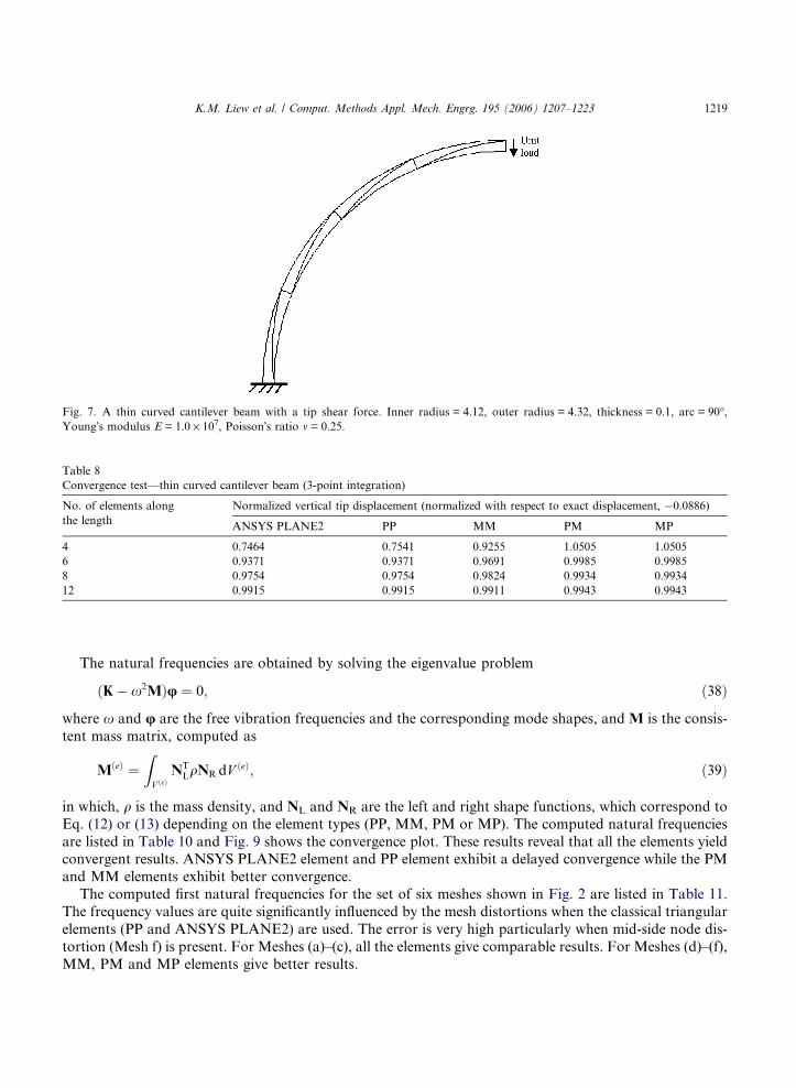
Fig. 7. A thin curved cantilever beam with a tip shear force. Inner radius = 4.12, outer radius = 4.32, thickness = 0.1, arc = 90�,Young�s modulus E = 1.0 · 107, Poisson�s ratio m = 0.25.

Table 8

Convergence test—thin curved cantilever beam (3-point integration)

No. of elements along

the length

Normalized vertical tip displacement (normalized with respect to exact displacement, �0.0886)


4 0.7464 0.7541 0.9255 1.0505 1.0505

6 0.9371 0.9371 0.9691 0.9985 0.9985

8 0.9754 0.9754 0.9824 0.9934 0.9934

12 0.9915 0.9915 0.9911 0.9943 0.9943


The natural frequencies are obtained by solving the eigenvalue problem

ðK� x2MÞu ¼ 0; ð38Þ

where x and u are the free vibration frequencies and the corresponding mode shapes, and M is the consis-

tent mass matrix, computed as

MðeÞ ¼ZV ðeÞ

NTLqNR dV ðeÞ; ð39Þ

in which, q is the mass density, and NL and NR are the left and right shape functions, which correspond to

Eq. (12) or (13) depending on the element types (PP, MM, PM or MP). The computed natural frequencies

are listed in Table 10 and Fig. 9 shows the convergence plot. These results reveal that all the elements yieldconvergent results. ANSYS PLANE2 element and PP element exhibit a delayed convergence while the PM

and MM elements exhibit better convergence.

The computed first natural frequencies for the set of six meshes shown in Fig. 2 are listed in Table 11.

The frequency values are quite significantly influenced by the mesh distortions when the classical triangular

elements (PP and ANSYS PLANE2) are used. The error is very high particularly when mid-side node dis-

tortion (Mesh f) is present. For Meshes (a)–(c), all the elements give comparable results. For Meshes (d)–(f),

MM, PM and MP elements give better results.

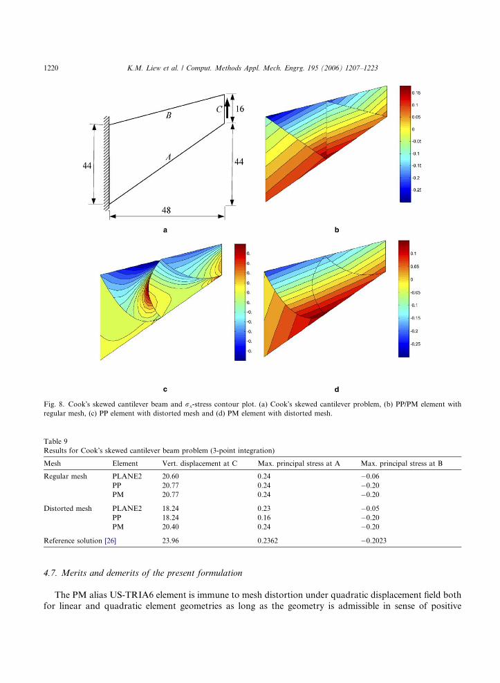
Fig. 8. Cook�s skewed cantilever beam and rx-stress contour plot. (a) Cook�s skewed cantilever problem, (b) PP/PM element with

regular mesh, (c) PP element with distorted mesh and (d) PM element with distorted mesh.

Table 9

Results for Cook�s skewed cantilever beam problem (3-point integration)

Mesh Element Vert. displacement at C Max. principal stress at A Max. principal stress at B

Regular mesh PLANE2 20.60 0.24 �0.06

PP 20.77 0.24 �0.20

PM 20.77 0.24 �0.20

Distorted mesh PLANE2 18.24 0.23 �0.05

PP 18.24 0.16 �0.20

PM 20.40 0.24 �0.20

Reference solution [26] 23.96 0.2362 �0.2023


4.7. Merits and demerits of the present formulation

The PM alias US-TRIA6 element is immune to mesh distortion under quadratic displacement field both

for linear and quadratic element geometries as long as the geometry is admissible in sense of positive

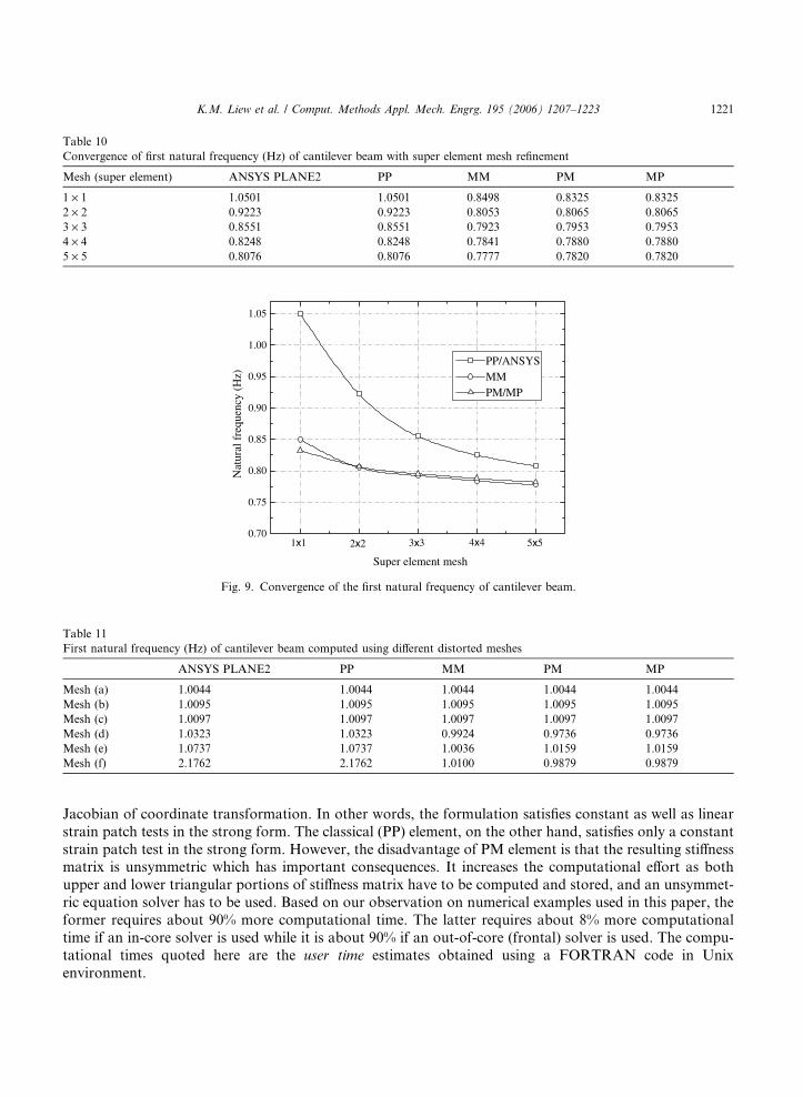
Table 10

Convergence of first natural frequency (Hz) of cantilever beam with super element mesh refinement

Mesh (super element) ANSYS PLANE2 PP MM PM MP

1 · 1 1.0501 1.0501 0.8498 0.8325 0.8325

2 · 2 0.9223 0.9223 0.8053 0.8065 0.8065

3 · 3 0.8551 0.8551 0.7923 0.7953 0.7953

4 · 4 0.8248 0.8248 0.7841 0.7880 0.7880

5 · 5 0.8076 0.8076 0.7777 0.7820 0.7820

0.70

0.75

0.80

0.85

0.90

0.95

1.00

1.05

5x54x43x32x21x1

Nat

ural

fre

quen

cy (

Hz)

Super element mesh

PP/ANSYS MM PM/MP

Fig. 9. Convergence of the first natural frequency of cantilever beam.

Table 11

First natural frequency (Hz) of cantilever beam computed using different distorted meshes


Mesh (a) 1.0044 1.0044 1.0044 1.0044 1.0044

Mesh (b) 1.0095 1.0095 1.0095 1.0095 1.0095

Mesh (c) 1.0097 1.0097 1.0097 1.0097 1.0097

Mesh (d) 1.0323 1.0323 0.9924 0.9736 0.9736

Mesh (e) 1.0737 1.0737 1.0036 1.0159 1.0159

Mesh (f) 2.1762 2.1762 1.0100 0.9879 0.9879


Jacobian of coordinate transformation. In other words, the formulation satisfies constant as well as linear

strain patch tests in the strong form. The classical (PP) element, on the other hand, satisfies only a constant

strain patch test in the strong form. However, the disadvantage of PM element is that the resulting stiffnessmatrix is unsymmetric which has important consequences. It increases the computational effort as both

upper and lower triangular portions of stiffness matrix have to be computed and stored, and an unsymmet-

ric equation solver has to be used. Based on our observation on numerical examples used in this paper, the

former requires about 90% more computational time. The latter requires about 8% more computational

time if an in-core solver is used while it is about 90% if an out-of-core (frontal) solver is used. The compu-

tational times quoted here are the user time estimates obtained using a FORTRAN code in Unix

environment.


For regular meshes, PM and PP elements yield the same accuracy of results while PM element demands

more computational time, and thus PM element is less effective than PP element. For distorted meshes,

however, PM element yields a better accuracy than PP element although it does demand more computa-

tional effort. In other words, for distorted meshes, the increased computational effort demanded by PM

element is partially reimbursed in terms of the increased in accuracy of the solution.

5. Conclusions

The unsymmetric formulation [10] is extended to the 6-node triangular plane element. A few typical

numerical examples have been solved to assess the distortion-tolerance of the element in static and free

vibration applications. In contrast to the classical (PP) element, the new element is immune to all types

of admissible distortions for all the quadratic displacement field problems considered. In particular, thenew element has been able to reproduce the exact displacement and stress solution for angular, curved-edge

and mid-side node mesh distortions under quadratic displacement field. In free vibration analysis, the pres-

ent element gives more accurate natural frequencies as compared to the classical 6-node triangular plane

element.

References

[1] B. Fraeus de Veubeke, Displacement and equilibrium models in the finite element method, in: O.C. Zienkiewiczs, G.S. Holister

(Eds.), Stress Analysis, Wiley, London, 1965.

[2] J.H. Bramble, M. Zlamal, Triangular elements in the finite element method, Math. Comput. 24 (1970) 809–810.

[3] I. Babuska, A.K. Aziz, On the angle condition in finite element method, SIAM J. Numer. Anal. 13 (1976) 214–227.

[4] D.J. Burrows, A finite element shape sensitivity study, in: K.J. Bathe, D.R.J. Owen (Eds.), Reliability of Methods for Engineering

Analysis, Pineridge Press, Swansea, 1986, pp. 439–456.

[5] J. Robinson, Distortion measures for quadrilaterals with curved boundaries, Finite Elem. Anal. 4 (1988) 115–131.

[6] J. Barlow, More on optimal stress points—reduced integration, element distortions and error estimation, Int. J. Numer. Methods

Engng. 28 (1989) 1487–1504.

[7] P. Hansbo, Generalized Laplacian smoothing of structured grids, Commun. Numer. Methods Engng. 11 (1995) 455–464.

[8] L. Freitag, M. Jones, P. Plassmann, An efficient parallel algorithm for mesh smoothing, Fourth International Meshing

Roundtable, Albuquerque, NM, USA, 1995.

[9] W.H. Frey, D.A. Field, Mesh relaxation: a new technique for improving triangulations, Int. J. Numer. Methods Engng. 31 (1991)

1121–1133.

[10] S. Rajendran, K.M. Liew, A novel unsymmetric 8-node plane element immune to mesh distortion under a quadratic displacement

field, Int. J. Numer. Methods Engng. 58 (2003) 1713–1748.

[11] S. Rajendran, S. Subramanian, Distortion sensitivity of 8-node plane elasticity elements based on parametric, metric, parametric–

metric and metric–parametric formulations, Struct. Engng. Mech. 17 (2004) 767–788.

[12] E.T. Ooi, S. Rajendran, J.H. Yeo, A 20-node hexahedral element with enhanced distortion tolerance, Int. J. Numer. Methods

Engng. 60 (2004) 2501–2530.

[13] N.S. Lee, K.J. Bathe, Effects of element distortions on the performance of isoparametric elements, Int. J. Numer. Methods Engng.

36 (1993) 3553–3576.

[14] S.N. Lautersztajn, A. Samuelsson, Further discussion on four-node isoparametric quadrilateral elements in plane bending, Int. J.

Numer. Methods Engng. 47 (2000) 129–140.

[15] E.L. Wilson, R.L. Taylor, W.P. Doherty, J. Ghaboussi, Incompatible displacement models, in: S.J. Fenves et al. (Eds.),

Numerical and Computational Methods in Structural Mechanics, Academic Press, New York, 1973, pp. 43–57.

[16] R.L. Taylor, P.J. Beresford, E.L. Wilson, A nonconforming element for stress analysis, Int. J. Numer. Methods Engng. 10 (1976)

1211–1219.

[17] T.H.H. Pian, K. Sumihara, Rational approach for assumed stress finite elements, Int. J. Numer. Methods Engng. 20 (1984) 1685–

1695.

[18] J.C. Simo, M.S. Rifai, A class of assumed strain methods and the method of incompatible modes, Int. J. Numer. Methods Engng.

29 (1990) 1595–1638.


[19] S.T. Yeo, B.C. Lee, New stress assumption for hybrid stress elements and refined four-node plane and eight-node brick elements,

Int. J. Numer. Methods Engng. 40 (1997) 2933–2952.

[20] K.Y. Sze, On immunizing five-beta hybrid stress element models from �trapezoidal locking� in practical analyses, Int. J. Numer.

Methods Engng. 47 (2000) 907–920.

[21] J. Korelc, P. Wriggers, Improved enhanced strain four-node element with Taylor expansion of the shape functions, Int. J. Numer.

Methods Engng. 40 (1997) 407–421.

[22] Y.P. Cao, N. Hu, J. Lu, H. Fukunaga, Z.H. Yao, A 3D brick element based on Hu–Washizu variational principle for mesh

distortion, Int. J. Numer. Methods Engng. 53 (2002) 2529–2548.

[23] J.A. Teixeira de Freitas, C. Cismas�iu, Numerical implementation of hybrid-Trefftz displacement elements, Comput. Struct.

73 (1999) 207–225.

[24] J.A. Teixeira de Freitas, F.L.S. Bussamra, Three-dimensional hybrid-Trefftz stress elements, Int. J. Numer. Methods Engng.

47 (2000) 927–950.

[25] C.K. Choi, T.Y. Lee, K.Y. Chung, Direct modification for non-conforming elements with drilling DOF, Int. J. Numer. Methods

Engng. 55 (2002) 1463–1476.

[26] X.M. Chen, S. Cen, Y.Q. Long, Z.H. Yao, Membrane elements insensitive to distortion using the quadrilateral area coordinate

method, Comput. Struct. 82 (2004) 35–54.

[27] S. Rajendran, K.M. Liew, Completeness requirements of shape functions for higher order finite elements, Struct. Eng. Mech.

10 (2000) 93–110.

[28] O.C. Zienkiewicz, R.L. Taylor, The Finite Element Method, vol. 1: Basic Formulation and Linear Problems, fourth ed., McGraw-

Hill Book Company, London, 1989.

[29] R.H. MacNeal, R.L. Harder, A proposed standard set of problems to test finite element accuracy, Finite Elem. Anal. Des.

1 (1985) 3–20.

[30] R.D. Cook, D.S. Malkus, M.E. Plesha, Concepts and Applications of Finite Element Analysis, third ed., John Wiley & Sons,

New York, 1989.

Documents

A quadratic plane triangular element immune to quadratic mesh distortions under quadratic displacement fields