Convolution surfaces of quadratictriangular Bezier surfaces

Martin Peternell Boris Odehnal

March 8, 2007

Abstract

In the present paper we prove that the polynomial quadratic triangular Bezier sur-faces are LN-surfaces. We demonstrate how to reparameterize the surfaces such thatthe normals obtain linear coordinate functions. The close relation to quadratic Cre-mona transformations is elucidated. These reparameterizations can be effectivelyused for the computation of convolution surfaces.

Keywords: Quadratic Bezier triangle, LN-surface, reparameterization, Cremona transfor-mation, convolution surface.

1 Introduction

Quadratic triangular Bezier surfaces are a well explored area, and many textbooks onCAGD, e.g. [6, 8] are covering this topic. Thus one may wonder what else can be saidabout them? Surprisingly, in connection with the computation of convolution surfacesit has been proved recently in [12] that the convolution surfaces of quadratic triangularBezier surfaces and any arbitrary rational surface are always rational. This result is quitesurprising, since the rationality condition for the convolution surfaces is rather strong.One direct consequence is that the offset surfaces of quadratic triangular Bezier surfacesare rational surfaces. Unfortunately [12] does not disclose the geometric properties beingresponsible for the rationality of the convolution surfaces.

Earlier it has been proved in [23] that the convolution surface of an LN-surface and anarbitrary rational surface is always rational. LN-surfaces have been introduced in [9] anddenote a special class of surfaces whose normal vectors admit a linear parameterizationdepending on the surface parameters.

1

The main contribution of this article is to prove with geometric reasons that quadratictriangular Bezier surfaces are LN-surfaces and to study the geometric background of thisproperty. This brings the result of [12] in connection to what has been proved in [23].This property is not immediately seen from the standard parameterization, but geomet-ric considerations concerning the structure of the family of their tangent planes lead toreparameterizations proving this fact. These special parameterizations simplify the com-putation of convolution surfaces.

The notion of convolution appears in two different ways: In computer graphics a con-volution surface is defined as level set of an implicit function f(x) = g(x) ? h(x) =∫

R3 g(t)h(x−t)dt, called the convolution of the geometry function g and the kernel functionh, see [3, 17, 26].

In geometric modeling the convolution surface of two surfaces F and G in Euclidean three-space R3 is defined by

F ? G = {f + g|f ∈ F,g ∈ G,nF ‖ nG}, (1)

where f(u, v) and g(s, t) are the respective parameterizations and nF and nG are therespective normal vectors of f and g, see e.g. [13, 14, 16].

Geometrically speaking one forms the sum f + g of vectors for those points whose normalvectors are parallel. Considering G as family of translations, the convolution surface F ?Gis the envelope of F under the translations defined by vectors g. In general we cannotexpect that F and G are parameterized in a way that their normal vectors nF = f,u × f,vand nG = g,s×g,t are parallel for (u, v) = (s, t). Typically it is necessary to reparameterizeone of the input surfaces, say G.

Assume that f(u, v) and g(s, t) are rational parameterizations. The question arises in whichcases the convolution surface F ? G again admits a rational parameterization. It turnedout in [18] and [23] that F ? G is rationally parameterized if F is a paraboloid or moregeneral an LN-surface and G is any rational surface. Earlier it was shown in [16] that tworational skew ruled surfaces F and G always yield a rational convolution surface F ? G.These results already indicate that the rationality of the convolution surface is in closerelation to the structure of the families of tangent planes of F and G.

This topic is related to the question which rational surfaces possess rational offset surfaces.Surfaces with rational offsets are called PN-surfaces and their unit normal vectors are arational parameterization of the Euclidean unit sphere S2. An explicit construction of thesesurfaces has been given in [20] and several surprising examples are given in [19]. Rationaloffsets of LN-surfaces are discussed in [10]. An approach using classical geometries forNURBS curves and surfaces is presented in [21].

The paper is organized as follows: Section 2 explains some geometric properties of LN-surfaces, quadratic triangular Bezier surfaces, the Veronese surface V 2

2 and its projections.In Section 3 we discuss the dual representation of quadratic triangular Bezier surfaces

2

and the computation of base points is explained too. After that planar quadratic Cremonatransformations follow in Section 4, which are the key to the reparameterization. In Section5 we give a proof of the LN-property of quadratic triangular Bezier surfaces. A syntheticproof of this property can already be found in Section 2.4. Section 6 contains examples ofthe reparameterization and of the convolution surface of two quadratic triangular Beziersurfaces. Finally we conclude in Section 8.

2 Geometric background

Points in R3 are represented by their coordinate vectors x = (x, y, z). The projectiveclosure of R3 is denoted by P3 and points in P3 are identified with their homogeneouscoordinate vectors

xR = (x0, x1, x2, x3)R = (x0 : x1 : x2 : x3), with x 6= o.

Choosing the plane at infinity ω as x0 = 0, the interchange between homogeneous andCartesian coordinates for points in R3 is realized by

x =x1

x0

, y =x2

x0

, z =x3

x0

. (2)

Similarly we use (u, v) as affine coordinates in the parameter plane R2 and (u0 : u1 : u2)as homogeneous coordinates in the projective closure P2 of R2. The analogous relationbetween affine and homogeneous parameters reads

u =u1

u0

, v =u2

u0

. (3)

Moreover, we have to consider the dual projective space P3?, whose points are identifiedwith the family of planes in P3. Let e0 + e1x + e2y + e3z = 0 be the equation of a plane E.The homogeneous coordinate vector Re = R(e0, e1, e2, e3) is identified with E. If especiallyE : h + ux + vy + z = 0 is given as graph of a linear function, we may use the affinecoordinates (h, u, v) of E too.

2.1 LN-surfaces

A rational surface S is called an LN-surface if there exists a rational parameterizations(u, v) such that a normal vector field n(u, v) of S can be linearly parameterized as

n(u, v) = pu + qv + r, (4)

where p, q, and r are vectors in R3. A particular parameterization s(u, v) of S may notshow the LN-property (4) at once. A rational reparameterization may be required.

3

Depending on the rank of M := (p,q, r) we have to distinguish the following cases: Ifrk M = 1, S is a part of a plane and if rk M = 2 the unit normals n0 = n/‖n‖ of Sare contained in a great circle on the Euclidean unit sphere S2. This implies that S iscontained in a cylinder.

In the following we assume rk M = 3. This implies that the unit normal vectors of Sparameterize a two-dimensional subset of S2. An appropriate choice of the coordinatesystem yields

p = (1, 0, 0)T , q = (0, 1, 0)T , r = (0, 0, 1)T ,

and the normal vector simplifies to n(u, v) = (u, v, 1)T . Thus the tangent planes T (u, v)of an LN-surface allow the quite simple representation

T (u, v) : h(u, v) + ux + vy + z = 0, (5)

where h(u, v) is a rational function (support function of T ). With respect to the chosencoordinate system, the tangent planes T (u, v) are graphs of linear functions over the [x, y]-plane. The representation (5) allows to treat (u, v, h(u, v)) as affine coordinates of T . Using(U, V,W ) as coordinate functions of planes, the dual affine equation of an LN-surface S isW = h(U, V ). This representation says that LN-surfaces are graphs of rational functionsin an affine part of dual projective space P3?

.

Assume that S is of class n, i.e. the number of tangent planes of S passing through a genericline is n. Then the numerator a and denominator b of h are polynomials of degrees k andl, respectively. We change from affine coordinates U, V,W to homogeneous coordinatesY0, Y1, Y2, Y3 by letting U = Y1/Y3, V = Y2/Y3, W = Y0/Y3. Inserting this into W =h(U, V ) = a(U, V )/b(U, V ) and multiplying with Y n

3 leads to the homogeneous polynomialequation

S : Y0Yk−l−13 b(Y1, Y2, Y3)− a(Y1, Y2, Y3) = 0, if k ≥ l + 1,

S : Y0 b(Y1, Y2, Y3)− Y l+1−k3 a(Y1, Y2, Y3) = 0, if l + 1 ≥ k. (6)

One might call (6) the dual equation of S. Consider the polynomial in (6) which is sortedwith respect to powers of Y0. All partial derivatives up to order n − 2 with respect toY0, . . . , Y3 vanish at (1, 0, 0, 0). This says that the plane at infinity ω = R(1, 0, 0, 0) withequation x0 = 0 is an n− 1-fold plane of S.

This property has the following important consequence: For any vector n = (u, v, 1)T thereexists a unique tangent plane T (u, v) of S having n as normal vector and there exists exactlyone point of contact of S and T . In other words: for any plane E : z = ax+by+c in R3 thereexists exactly one tangent plane T of S with E ‖ T and a unique point of contact. Thisunique-tangent-plane-property is the reason for the rationality of the convolution surfaceswith any arbitrary rational surface which has been proved in [23]. We say that a surface Ssatisfies the LN-property (4) if the tangent planes T (u, v) of S admit a representation (5).

We summarize these results:

4

Lemma 1 The family of tangent planes T (u, v) of an LN-surface S can be representedin plane coordinates by the graph (u, v, h(u, v)) of a rational function h. The plane atinfinity is an n−1-fold tangent plane of S and this property (6) characterizes LN-surfaces.Conversely, the graph of a rational function represents the tangent planes (5) of an LN-surface. The convolution surfaces S ? F of an LN-surface S and any arbitrary rationalsurface F are rational.

A particular parametric representation s(u, v) of a surface S may not show the LN-propertydirectly. An appropriate reparameterization may be necessary. Admissible reparameteri-zations are so called Cremona transformations which will be explained in Section 4.

2.2 Quadratic triangular Bezier surfaces

Let u = (u0 : u1 : u2) be homogeneous coordinates in the projective plane P2. A surface Qin projective 3-space P3 admitting a parameterization of the form

q(u)R = (q0(u), . . . , q3(u))R, (7)

where qi(u) are homogeneous quadratic polynomials, is called a quadratically parameterize-able surface. These so-called Steiner surfaces form a remarkable class of rational surfacesof order four and class three which have attracted the interest of mathematicians in thepast [11, 15, 27, 28, 29, 30] and also nowadays [1, 2, 4, 5, 22, 25].

By letting q0(u) = u20 one obtains the family of polynomial quadratically parameterizeable

surfaces. Dividing q1, q2, q3 by q0 and changing from homogeneous parameters (u0 : u1 : u2)to affine coordinates (u, v) by (2), the representation (7) becomes the familiar parameter-ization

s(u, v) =1

2au2 + buv +

1

2cv2 + du + ev + f. (8)

The vectors a, b, c, d, e, and f in R3 comprise the coefficients of the polynomials qi. Ingeneral these surfaces contain a two-parameter family of parabolas (curves of degree two)corresponding to the lines in the [u, v]-plane. An example of this kind of surface can beseen in Fig. 1.

These surfaces are frequently called quadratic Bezier triangles and admit quadratic pa-rameterizations in terms of barycentric coordinates with respect to a triangle in the affineparameter plane R2 [8].

2.3 Veronese variety

The surfaces (8) can be parameterized over the affine plane as well as over the projectiveplane. For the moment let S be parameterized over the projective plane with coordinates

5

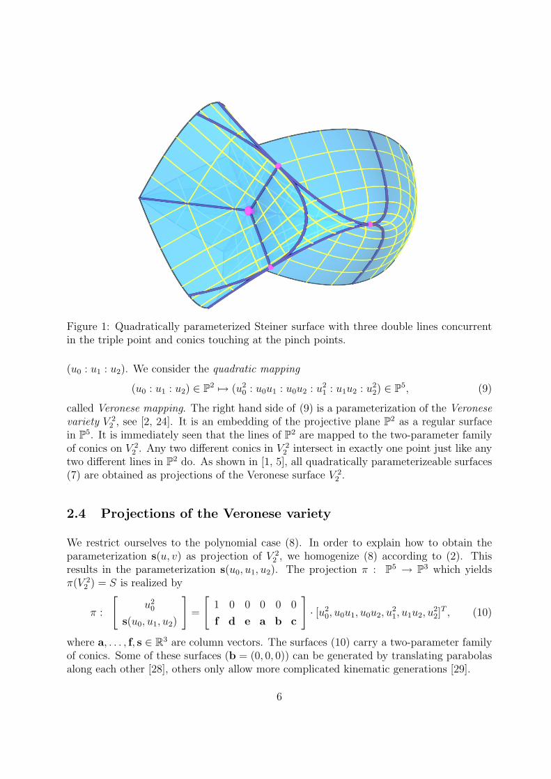
Figure 1: Quadratically parameterized Steiner surface with three double lines concurrentin the triple point and conics touching at the pinch points.

(u0 : u1 : u2). We consider the quadratic mapping

(u0 : u1 : u2) ∈ P2 7→ (u20 : u0u1 : u0u2 : u2

1 : u1u2 : u22) ∈ P5, (9)

called Veronese mapping. The right hand side of (9) is a parameterization of the Veronesevariety V 2

2 , see [2, 24]. It is an embedding of the projective plane P2 as a regular surfacein P5. It is immediately seen that the lines of P2 are mapped to the two-parameter familyof conics on V 2

2 . Any two different conics in V 22 intersect in exactly one point just like any

two different lines in P2 do. As shown in [1, 5], all quadratically parameterizeable surfaces(7) are obtained as projections of the Veronese surface V 2

2 .

2.4 Projections of the Veronese variety

We restrict ourselves to the polynomial case (8). In order to explain how to obtain theparameterization s(u, v) as projection of V 2

2 , we homogenize (8) according to (2). Thisresults in the parameterization s(u0, u1, u2). The projection π : P5 → P3 which yieldsπ(V 2

2 ) = S is realized by

π :

[u2

0

s(u0, u1, u2)

]=

[1 0 0 0 0 0

f d e a b c

]· [u2

0, u0u1, u0u2, u21, u1u2, u

22]

T , (10)

where a, . . . , f, s ∈ R3 are column vectors. The surfaces (10) carry a two-parameter familyof conics. Some of these surfaces (b = (0, 0, 0)) can be generated by translating parabolasalong each other [28], others only allow more complicated kinematic generations [29].

6

Let ω : x0 = 0 be the plane at infinity in the projective extension P3 of R3 and let c = S∩ωbe the curve at infinity of S. From the projection (10) it follows that c is obtained by u2

0 = 0.This implies that c is a double curve parameterized by

(au21 + 2bu1u2 + cu2

2)R ∈ ω.

Here (u1 : u2) is considered as homogeneous parameter on c. For linearly independentvectors a, b, and c one obtains conics, otherwise c is degenerate.

This proves again that ω is a tangent plane of multiplicity two. Since triangular quadraticBezier surfaces are of class three, the dual equation of S looks like (6). The geometricmeaning is the following: Let g ∈ P3 be a line in general position to S. Algebraicallycounting, there exist three tangent planes of S passing through g. Thus for any lineh ∈ ω in general position there is exactly one tangent plane T 6= ω passing through h.These synthetic geometric considerations already prove the LN-property of the triangularquadratic Bezier surfaces.

Corollary 2 Quadratic triangular Bezier surfaces are LN-surfaces.

Although these ideas do not lead immediately to LN-parameterizations, their existenceis shown. We will present a more constructive proof of the LN-property of triangularquadratic Bezier surfaces. Therefore we investigate the normal vectors associated to theparameterization (8) and show explicitly that there exist reparameterizations of S in orderto obtain linearly parameterized normal vectors.

3 Dual representation of triangular quadratic Bezier

surfaces

To prove the LN-property of a triangular quadratic Bezier surface S we have to investigatethe structure of the family of tangent planes. Using the affine parameterization (8) thepartial derivatives of s with respect to u and v are

s,u(u, v) = au + bv + d, s,v(u, v) = bu + cv + e. (11)

The tangent planes T (u, v) of S are given by

T (u, v) : (x− s(u, v))T · (s,u × s,v)(u, v) = 0, (12)

with support function h = −det(s, s,u, s,v) and normal vector s,u × s,v. The partial deriva-tives s,u and s,v define affine mappings in the [u, v]-plane. These mappings can be ex-tended to projective mappings p, q : P2 → P2. Defining the matrices P := (d, a,b) andQ := (e,b, c), the projective mappings read

p : uR 7→ (Pu)R, q : uR 7→ (Qu)R, with u = (u0, u1, u2)T . (13)

7

Let u?R be a point in P2. If rk (Pu?, Qu?) = 1, then n(u?) = (0, 0, 0)T and t(u?) =(0, 0, 0, 0)T holds. Thus we say that the parameterization t(u) of the tangent planes T (orthe parameterization n(u) of the normal vector) has a base point at u?R if and only if thevectors Pu? and Qu? are linearly dependent.

Excluding planar and cylindrical surfaces S we can assume that the matrices P and Qfrom (13) are not scalar multiples of each other and that rk P ≥ 2 as well as rk Q ≥ 2.Base points allow degree reductions of parameterizations. Thus it is the key point of thereparameterization to detect the base points u?R of the parameterization t(u) of the familyof tangent planes.

3.1 Computation of the base points

Let S be a triangular quadratic Bezier surface parameterized by (8) and let p and q bethe projective mappings defined by (13). The computation of the base points of the dualparameterization distinguishes between the following cases, depending on the ranks of thematrices P and Q.

A

Y1 Y2

X1 X2

p−1(Y1) p−1(Y2)

q−1(a)

a = im p

AB

C

D

x = p−1(D) y = q−1(D)

a = im p

b = im q

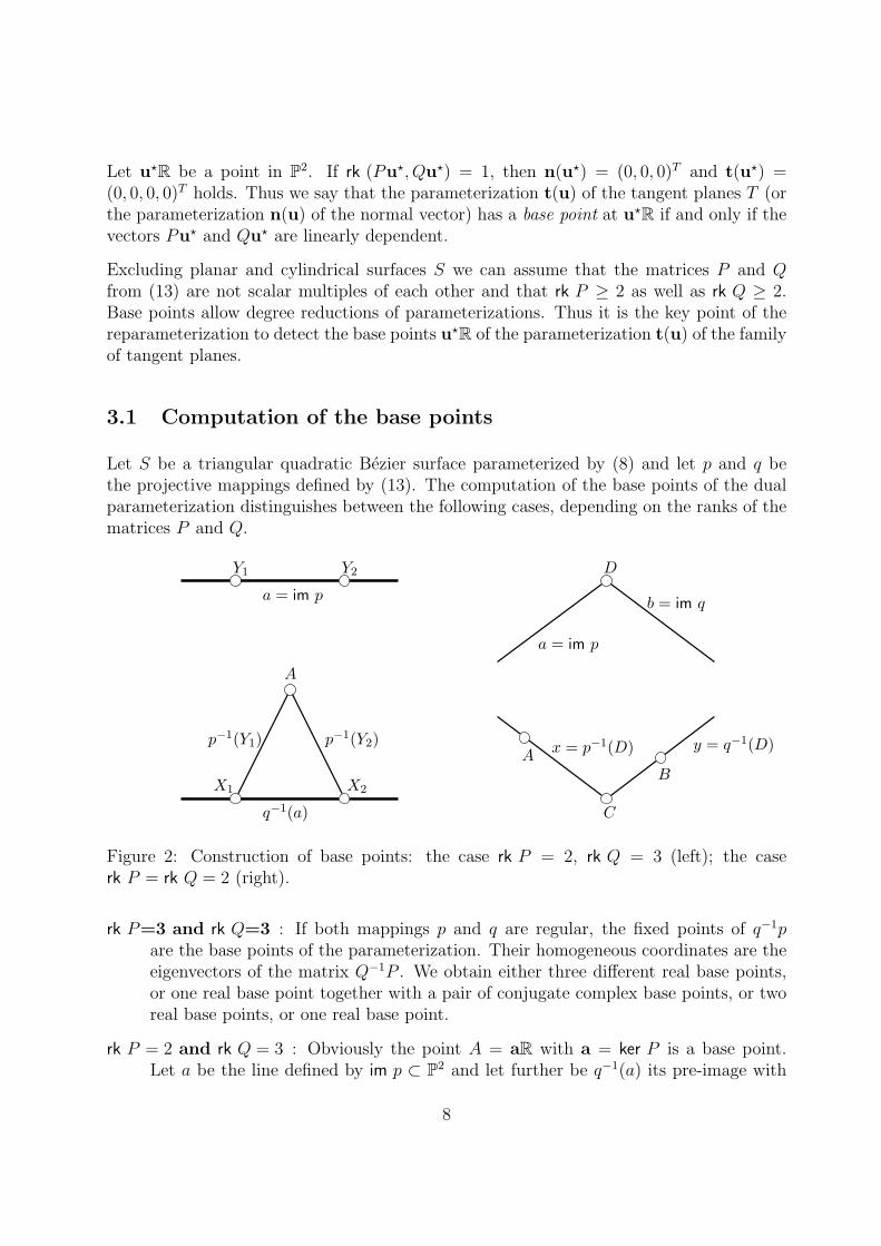
Figure 2: Construction of base points: the case rk P = 2, rk Q = 3 (left); the caserk P = rk Q = 2 (right).

rk P=3 and rk Q=3 : If both mappings p and q are regular, the fixed points of q−1pare the base points of the parameterization. Their homogeneous coordinates are theeigenvectors of the matrix Q−1P . We obtain either three different real base points,or one real base point together with a pair of conjugate complex base points, or tworeal base points, or one real base point.

rk P = 2 and rk Q = 3 : Obviously the point A = aR with a = ker P is a base point.Let a be the line defined by im p ⊂ P2 and let further be q−1(a) its pre-image with

8

respect to q. The restriction of q to q−1(a) is a projective mapping and there is eitherone point X1 or there are two (real or a pair of conjugate complex) points X1 andX2 both contained in q−1(a) with p(Xi) = q(Xi) = Yi, see Fig. 2.

Note that q−1(a) may pass through A. Finally we obtain either three real basepoints, or one real base point, or a pair of conjugate complex base points, two realbase points, or one real base point.

If rk P = 3 and rk Q = 2 we interchange u and v in the parameterization of s andobtain the situation rk P = 2 and rk Q = 3.

rk P = 2, rk Q = 2 : The points A and B determined by ker P and ker Q respectively, arebase points. Let a and b be lines defined by im p and im q and let further D = a∩ b,see Fig. 2. There exist fiber lines x = p−1(D) and y = q−1(D) and C = x ∩ y is abase point of the construction. Since C = A or C = B is possible and even A = Bmight happen we obtain three, two or one real base points.

4 Quadratic Cremona transformations

In order to reparameterize the family of tangent planes we study quadratic Cremona trans-formations in the projective plane P2. Assume u = (u0 : u1 : u2) are homogeneous coor-dinates of points U in the projective plane P2. A mapping ϕ : P2 → P2 with U 7→ Vis called a quadratic Cremona transformation if the homogeneous coordinates vR of theimage points V can be expressed in the form

vR = (q0(u) : q1(u) : q2(u)) (14)

where qi are homogeneous quadratic polynomials and additionally the inverse ϕ−1 is ofthe same form. Because of the latter property Cremona transformations are often calledbirational.

Here we remark that qi cannot be prescribed independently. They have to satisfy certainrelations in order to define a birational transformation, see [7]. It is obvious that qi are theequations of conics in P2. From the theory of Cremona transformations we know that thesethree conics have to have three points in common. These points are called fundamentalpoints of the transformation and define their exceptional set. Sometimes it occurs thattwo or all three of the base points coincide. This gives rise to a projective classification ofquadratic planar Cremona transformations.

In the following we give a brief overview on certain sets of conics, namely pencils and nets, inthe projective plane in order to understand the geometry behind Cremona transformations.

9

4.1 Conics

It is well known that a conic k (or more generally speaking: a curve of degree two) canbe defined as the set of points X with homogeneous coordinate vectors xR = (x0, x1, x2)Rsatisfying a homogeneous quadratic polynomial equation

k : xT Kx = 0, (15)

where K is a symmetric 3×3-matrix with real entries. In order to avoid lengthy discussionswe view those subsets of P2 defined by singular matrices K also as conics and call themsingular. This includes pairs of lines (real ones or a pair of conjugate complex ones) ora single double line, depending on the normal form of K. If rk K = 3 and K is positivedefinite the curve k is empty (in the real projective plane).

4.2 Pencils of conics

Let k and l be two curves of degree two given by the respective equations k : xT Kx = 0and l : xT Lx = 0. The curves are assumed to be distinct which is guaranteed if K 6= λL.We call the set P of conics (including singular ones) defined by the linear combination

P : xT (κK + λL)x = 0 (16)

a pencil of conics. The pencil P can be spanned by any two different conics in it. Thesingular conics contained in P which correspond to the solutions (κ : λ) of the homogeneouscubic equation det(κK + λL) = 0 can also serve as base conics.

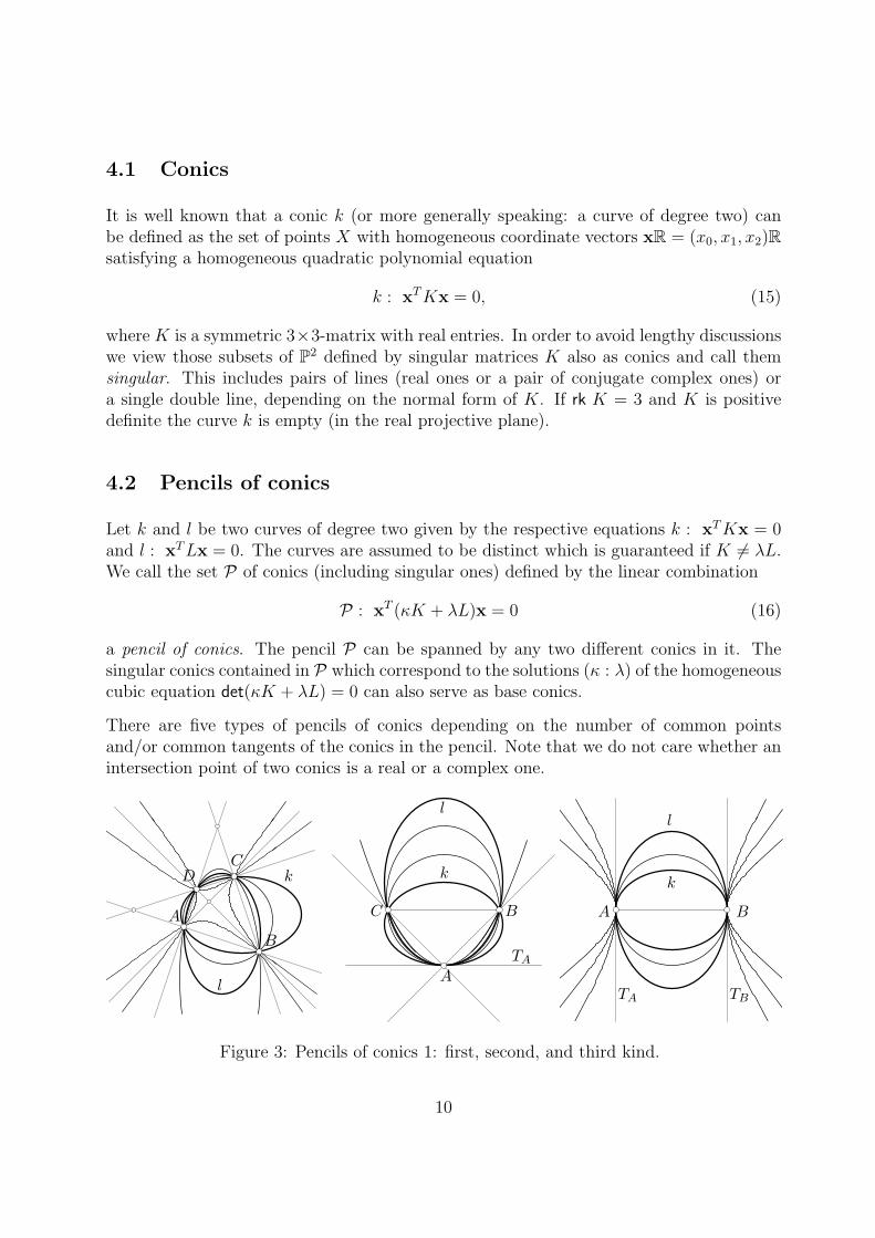
There are five types of pencils of conics depending on the number of common pointsand/or common tangents of the conics in the pencil. Note that we do not care whether anintersection point of two conics is a real or a complex one.

A

B

CD k

lA

BC

TA

k

l

A B

TA TB

k

l

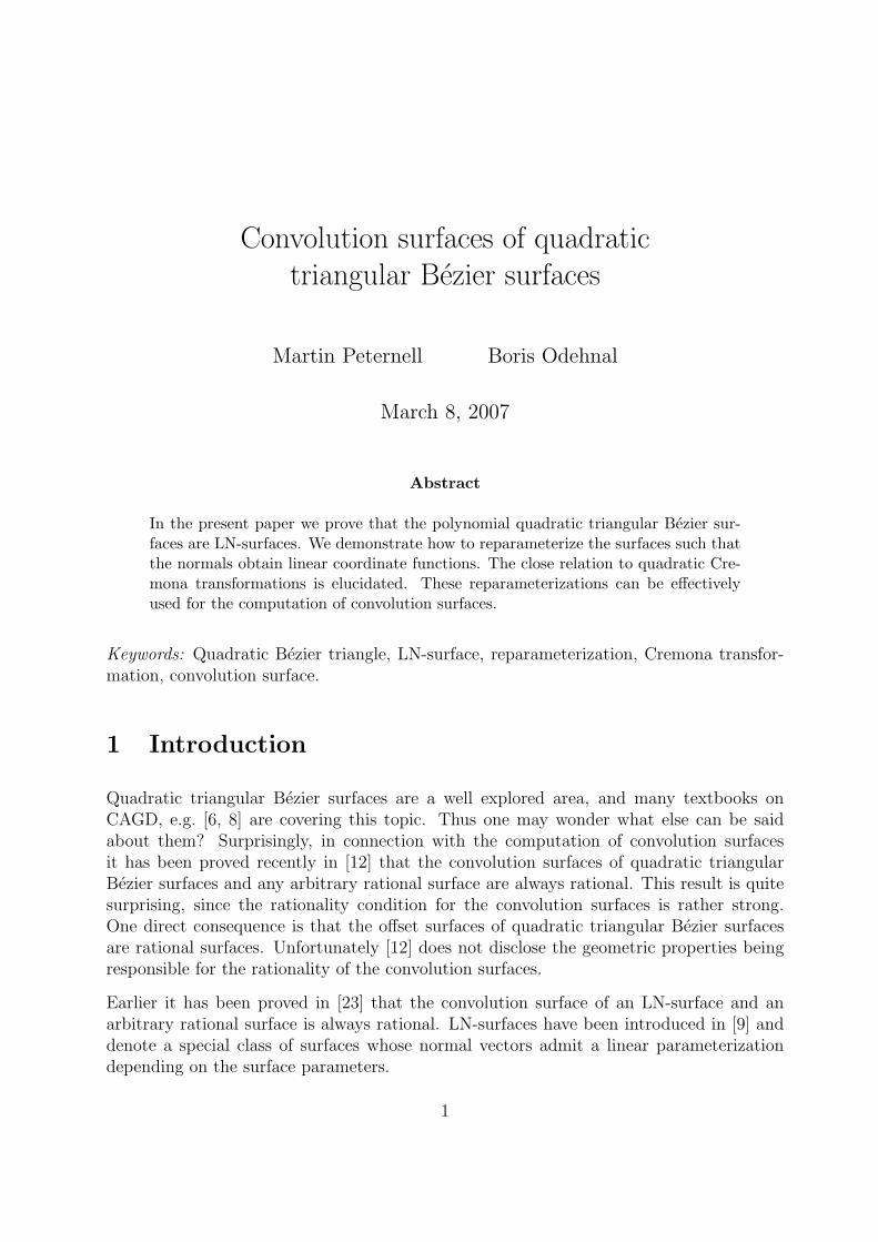
Figure 3: Pencils of conics 1: first, second, and third kind.

10

Four common points: Two conics k and l and thus all conics in the pencil share thepoints A, B, C, and D. These points form a quadrangle by obvious reasons. Thepencil P contains three different singular conics, i.e. three pairs of lines (AB, CD),(AC, BD), (AD, BC), see Fig. 3.

Two points and one line element: 1 Any two different conics k and l in P intersect atthe points A, B, and C while touching at A the common tangent TA. This pencilcontains two singular conics: the pairs of lines (BC, TA) and (AB, AC), see Fig. 3.

Two line elements: Any two conics k and l in P share the line elements (A, TA) and(B, TB), i.e. any two conics of P touch at A the line TA, analogoulsy at B the lineTB. The singular conics in this pencil are the double line AB and the pair (TA, TB)of lines, see Fig. 3.

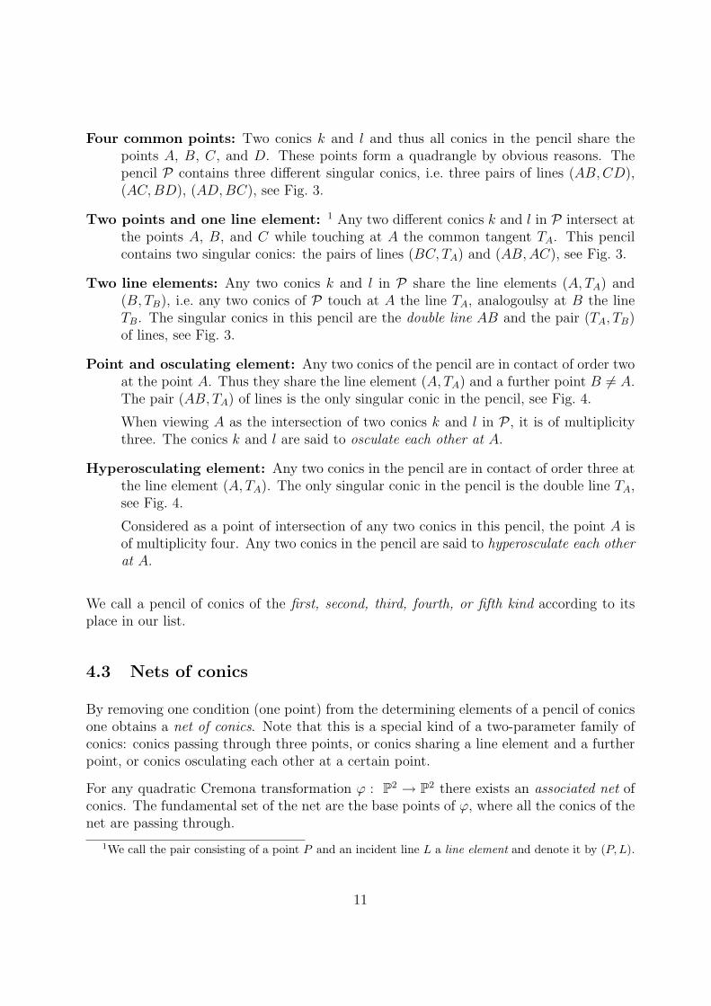
Point and osculating element: Any two conics of the pencil are in contact of order twoat the point A. Thus they share the line element (A, TA) and a further point B 6= A.The pair (AB, TA) of lines is the only singular conic in the pencil, see Fig. 4.

When viewing A as the intersection of two conics k and l in P , it is of multiplicitythree. The conics k and l are said to osculate each other at A.

Hyperosculating element: Any two conics in the pencil are in contact of order three atthe line element (A, TA). The only singular conic in the pencil is the double line TA,see Fig. 4.

Considered as a point of intersection of any two conics in this pencil, the point A isof multiplicity four. Any two conics in the pencil are said to hyperosculate each otherat A.

We call a pencil of conics of the first, second, third, fourth, or fifth kind according to itsplace in our list.

4.3 Nets of conics

By removing one condition (one point) from the determining elements of a pencil of conicsone obtains a net of conics. Note that this is a special kind of a two-parameter family ofconics: conics passing through three points, or conics sharing a line element and a furtherpoint, or conics osculating each other at a certain point.

For any quadratic Cremona transformation ϕ : P2 → P2 there exists an associated net ofconics. The fundamental set of the net are the base points of ϕ, where all the conics of thenet are passing through.

1We call the pair consisting of a point P and an incident line L a line element and denote it by (P,L).

11

A

B

TA

k

l

A

TA

k l

Figure 4: Pencils of conics 2: fourth and fifth kind

Conics through three points: We let A = (1 : 0 : 0), B = (0 : 1 : 0) and C = (0 : 0 : 1)be the three base points of the net of conics. It is spanned by the three pairs oflines x1x2 = 0, x2x0 = 0, and x0x1 = 0. Thus the general conic c of the net has theequation αx1x2 + βx2x0 + γx0x1 = 0, where (α : β : γ) 6= (0 : 0 : 0). The Cremonatransformation ϕ with this fundamental set and its inverse are given by

ϕ : (x0 : x1 : x2) 7→ (x′0 : x′

1 : x′2) = (x1x2 : x0x2 : x0x1), (17)

ϕ−1 : (x′0 : x′

1 : x′2) 7→ (x0 : x1 : x2) = (x′

1x′2 : x′

0x′2 : x′

0x′1).

The net of conics appearing here is obtained from a pencil of the first kind by removingone base point.

Conics through one point and one line element: We choose the line element A =(1 : 0 : 0) and a : x2 = 0 and the additional point B = (0 : 0 : 1). The net is spannedby the curves x1x2 = 0, x0x2 = 0, and x2

1 = 0. The generic equation of a curve ofthe net is αx1x2 + βx2x0 + γx2

1 = 0, where (α : β : γ) 6= (0 : 0 : 0). The thus definedCremona transformation and its inverse are given by

ϕ : (x0 : x1 : x2) 7→ (x′0 : x′

1 : x′2) = (x1x2 : x0x2 : x2

1), (18)

ϕ−1 : (x′0 : x′

1 : x′2) 7→ (x0 : x1 : x2) = (x′

1x′2 : x′

0x′2 : x′2

0 ).

The net of conics associated with this type of Cremona transformation is obtainedfrom a pencil of the second kind by removing one base point different from the pointof contact.

Osculating element: Consider the conic k : x21−x0x2 = 0 and the point A = (1 : 0 : 0).

The net is formed by all curves c of degree two osculating k at A. It is spannedby k and the pair of lines with equations x1x2 = 0 and x2

2 = 0. The Cremona

12

transformation and its inverse are given by

ϕ : (x0 : x1 : x2) 7→ (x′0 : x′

1 : x′2) = (x1x2 : x2

1 − x0x2 : x22), (19)

ϕ−1 : (x′0 : x′

1 : x′2) 7→ (x0 : x1 : x2) = (x′2

0 − x′1x

′2 : x′

0x′2 : x′2

2 ).

The associated net of conics is obtained from the pencil of conics of the fourth kindby removing the base point different from the point of osculation.

The pencils of third and fifth kind do not lead to base conics of quadratic Cremona trans-formations. Removing one base point removes all of them in case of a pencil of fifth kind.It leaves only two base points or a line element in the case of a pencil of third kind andthe set of conics through this elements is a three-parametric one.

A Cremona transformation ϕ maps a line g in general position to a conic ϕ(g) passingthrough the base points. Any conic c in general position is mapped to a rational curveϕ(c) of degree four. The conics of the associated net pass through the base points and arethus mapped to straight lines. This will help to reparameterize the tangent planes of aquadratically parameterizeable surface when proving the LN-property.

5 Proving the LN-property

Given a quadratic triangular Bezier surface S with polynomial parameterization (8) weshow that S satisfies the LN-property. This means that the tangent planes T (u, v) admita representation (5). The proof is splitted into two parts: At first let n = s,u × s,v

be a normal vector field of s. We show that the conics ni(u, v) = 0 determined by n’scoordinate functions define a net of conics. Second we give a practical reparameterizationmethod which is illustrated at hand of examples in Sec. 6.

Theorem 3 The conics ni(u, v) = 0, i = 1, 2, 3 form a net.

Proof: Assume S is parameterized by s from (8). The normal vector n(u, v) reads

n(u, v) = (a× b)u2 + (a× c)uv + (b× c)v2

+(a× e + d× b)u + (b× e + d× c)v + d× e. (20)

The coordinate functions of n define conics ni(u, v) = 0 in the [u, v]-plane. We showthat these conics form a net. Consider two conics n1(u, v) = 0 and n2(u, v) = 0. Theu-coordinates of their intersection points are the zeros of the resultant Res(n1,n2, v) of n1

and n2 with respect to v. We prove that the resultants Res(n1,n2, v), Res(n2,n3, v), and

13

Res(n1,n3, v) with respect to v share a cubic factor p(u) and thus there are three commonpoints (algebraically counted) of the conics ni = 0. The resultants are

Res(n1,n2, v) = (b3e3 − c3d3 + (b23 − a3c3)u)p(u), (21)

Res(n2,n3, v) = (b1e1 − c1d1 + (b21 − a1c1)u)p(u), (22)

Res(n1,n3, v) = (b2e2 − d2c2 + (b22 − a2c2)u)p(u). (23)

The zeros of p(u) determine the u-coordinates of three intersection points of any pair ofthe conics ni(u, v) = 0. The number and the multiplicity of intersection points in inde-pendent of the chosen coordinate system. This proves that the conics ni(u, v) = 0 sharethree points (algebraically counted) which are the base points of the corresponding Cre-mona transformation. The coefficients of the polynomial p(u) =

∑i ciu

i are listed below. �

In addendum we give the coefficients of the cubic polynomial p(u):

c3 = det(a,b, c)2,

c2 = det(a,b, c)(2det(b, c,d)− det(a, c, e)),

c1 = 2det(a,b, c)det(c,d, e) + det(a,b, e)det(b, c, e)

+det(b, c,d)2 − det(a, c,d)det(b, c, e)

c0 = det(b, c,d)det(c,d, e)− det(b, c, e)det(b,d, e)

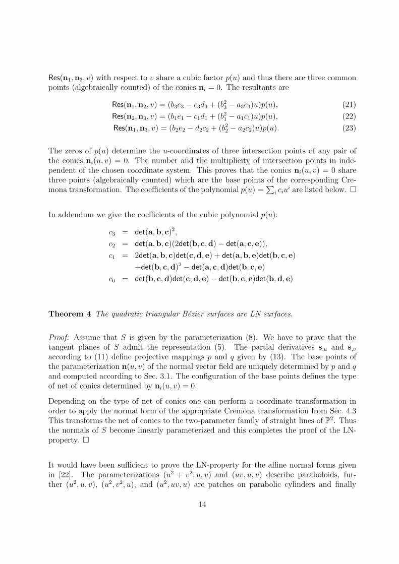
Theorem 4 The quadratic triangular Bezier surfaces are LN surfaces.

Proof: Assume that S is given by the parameterization (8). We have to prove that thetangent planes of S admit the representation (5). The partial derivatives s,u and s,v

according to (11) define projective mappings p and q given by (13). The base points ofthe parameterization n(u, v) of the normal vector field are uniquely determined by p and qand computed according to Sec. 3.1. The configuration of the base points defines the typeof net of conics determined by ni(u, v) = 0.

Depending on the type of net of conics one can perform a coordinate transformation inorder to apply the normal form of the appropriate Cremona transformation from Sec. 4.3This transforms the net of conics to the two-parameter family of straight lines of P2. Thusthe normals of S become linearly parameterized and this completes the proof of the LN-property. �

It would have been sufficient to prove the LN-property for the affine normal forms givenin [22]. The parameterizations (u2 + v2, u, v) and (uv, u, v) describe paraboloids, fur-ther (u2, u, v), (u2, v2, u), and (u2, uv, u) are patches on parabolic cylinders and finally

14

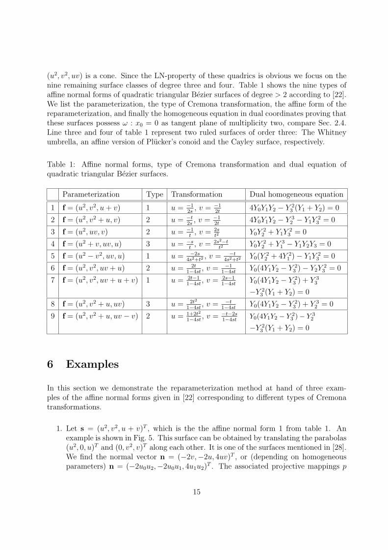
(u2, v2, uv) is a cone. Since the LN-property of these quadrics is obvious we focus on thenine remaining surface classes of degree three and four. Table 1 shows the nine types ofaffine normal forms of quadratic triangular Bezier surfaces of degree > 2 according to [22].We list the parameterization, the type of Cremona transformation, the affine form of thereparameterization, and finally the homogeneous equation in dual coordinates proving thatthese surfaces possess ω : x0 = 0 as tangent plane of multiplicity two, compare Sec. 2.4.Line three and four of table 1 represent two ruled surfaces of order three: The Whitneyumbrella, an affine version of Plucker’s conoid and the Cayley surface, respectively.

Table 1: Affine normal forms, type of Cremona transformation and dual equation ofquadratic triangular Bezier surfaces.

Parameterization Type Transformation Dual homogeneous equation

1 f = (u2, v2, u + v) 1 u = −12s

, v = −12t

4Y0Y1Y2 − Y 23 (Y1 + Y2) = 0

2 f = (u2, v2 + u, v) 2 u = −t2s

, v = −12t

4Y0Y1Y2 − Y 32 − Y1Y

23 = 0

3 f = (u2, uv, v) 2 u = −1t

, v = 2st2

Y0Y22 + Y1Y

23 = 0

4 f = (u2 + v, uv, u) 3 u = −st

, v = 2s2−tt2

Y0Y22 + Y 3

1 − Y1Y2Y3 = 0

5 f = (u2 − v2, uv, u) 1 u = −2s4s2+t2

, v = −t4s2+t2

Y0(Y22 + 4Y 2

1 )− Y1Y23 = 0

6 f = (u2, v2, uv + u) 2 u = 2t1−4st

, v = −11−4st

Y0(4Y1Y2 − Y 23 )− Y2Y

23 = 0

7 f = (u2, v2, uv + u + v) 1 u = 2t−11−4st

, v = 2s−11−4st

Y0(4Y1Y2 − Y 23 ) + Y 3

3

−Y 23 (Y1 + Y2) = 0

8 f = (u2, v2 + u, uv) 3 u = 2t2

1−4st, v = −t

1−4stY0(4Y1Y2 − Y 2

3 ) + Y 32 = 0

9 f = (u2, v2 + u, uv − v) 2 u = 1+2t2

1−4st, v = −t−2s

1−4stY0(4Y1Y2 − Y 2

3 )− Y 32

−Y 23 (Y1 + Y2) = 0

6 Examples

In this section we demonstrate the reparameterization method at hand of three exam-ples of the affine normal forms given in [22] corresponding to different types of Cremonatransformations.

1. Let s = (u2, v2, u + v)T , which is the the affine normal form 1 from table 1. Anexample is shown in Fig. 5. This surface can be obtained by translating the parabolas(u2, 0, u)T and (0, v2, v)T along each other. It is one of the surfaces mentioned in [28].We find the normal vector n = (−2v,−2u, 4uv)T , or (depending on homogeneousparameters) n = (−2u0u2,−2u0u1, 4u1u2)

T . The associated projective mappings p

15

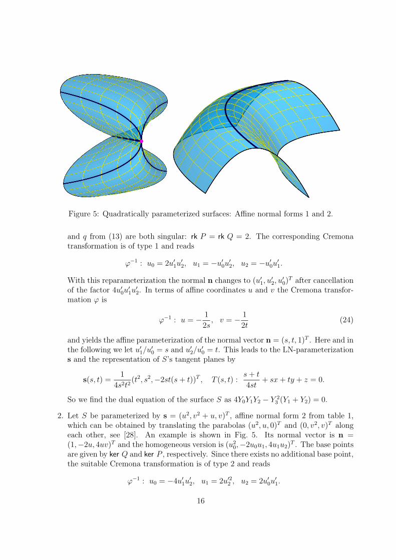
Figure 5: Quadratically parameterized surfaces: Affine normal forms 1 and 2.

and q from (13) are both singular: rk P = rk Q = 2. The corresponding Cremonatransformation is of type 1 and reads

ϕ−1 : u0 = 2u′1u

′2, u1 = −u′

0u′2, u2 = −u′

0u′1.

With this reparameterization the normal n changes to (u′1, u

′2, u

′0)

T after cancellationof the factor 4u′

0u′1u

′2. In terms of affine coordinates u and v the Cremona transfor-

mation ϕ is

ϕ−1 : u = − 1

2s, v = − 1

2t(24)

and yields the affine parameterization of the normal vector n = (s, t, 1)T . Here and inthe following we let u′

1/u′0 = s and u′

2/u′0 = t. This leads to the LN-parameterization

s and the representation of S’s tangent planes by

s(s, t) =1

4s2t2(t2, s2,−2st(s + t))T , T (s, t) :

s + t

4st+ sx + ty + z = 0.

So we find the dual equation of the surface S as 4Y0Y1Y2 − Y 23 (Y1 + Y2) = 0.

2. Let S be parameterized by s = (u2, v2 + u, v)T , affine normal form 2 from table 1,which can be obtained by translating the parabolas (u2, u, 0)T and (0, v2, v)T alongeach other, see [28]. An example is shown in Fig. 5. Its normal vector is n =(1,−2u, 4uv)T and the homogeneous version is (u2

0,−2u0u1, 4u1u2)T . The base points

are given by ker Q and ker P , respectively. Since there exists no additional base point,the suitable Cremona transformation is of type 2 and reads

ϕ−1 : u0 = −4u′1u

′2, u1 = 2u′2

2 , u2 = 2u′0u

′1.

16

The normal changes to (u′1, u

′2, u

′0)

T if we remove the dispensable factor 16u′22 u′

1. Interms of affine parameters ϕ reads

ϕ−1 : u = − t

2s, v = − 1

2t. (25)

and yields the affine LN-parameterization s of S and its tangent planes T

s(s, t) =1

4s2t2(t4, s(s− 2t3),−2s2t)T , T (s, t) :

s + t3

4st+ sx + ty + z = 0.

The dual equation of the surface reads 4Y0Y1Y2 − Y 32 − Y 2

3 Y1 = 0.

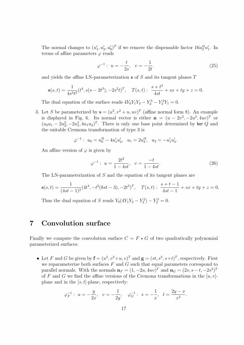
3. Let S be parameterized by s = (u2, v2 + u, uv)T (affine normal form 8). An exampleis displayed in Fig. 6. Its normal vector is either n = (u − 2v2,−2u2, 4uv)T or(u0u1 − 2u2

2,−2u21, 4u1u2)

T . There is only one base point determined by ker Q andthe suitable Cremona transformation of type 3 is

ϕ−1 : u0 = u′20 − 4u′

1u′2, u1 = 2u′2

2 , u2 = −u′1u

′2.

An affine version of ϕ is given by

ϕ−1 : u =2t2

1− 4st, v =

−t

1− 4st. (26)

The LN-parameterization of S and the equation of its tangent planes are

s(s, t) =1

(4st− 1)2(4t4,−t2(8st− 3),−2t3)T , T (s, t) :

s + t− 1

4st− 1+ sx + ty + z = 0.

Thus the dual equation of S reads Y0(4Y1Y2 − Y 23 )− Y 3

2 = 0.

7 Convolution surface

Finally we compute the convolution surface C = F ? G of two quadratically polynomialparameterized surfaces.

• Let F and G be given by f = (u2, v2+u, v)T and g = (st, s2, s+t)T , respectively. Firstwe reparameterize both surfaces F and G such that equal parameters correspond toparallel normals. With the normals nF = (1,−2u, 4uv)T and nG = (2s, s− t,−2s2)T

of F and G we find the affine versions of the Cremona transformations in the [u, v]-plane and in the [s, t]-plane, respectively:

ϕ−1F : u = − y

2x, v = − 1

2y, ϕ−1

G : s = −1

x, t =

2y − x

x2.

17

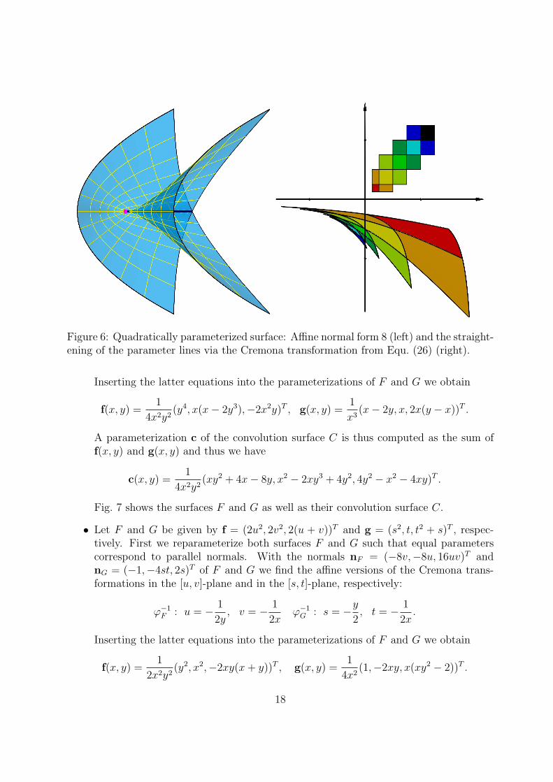
Figure 6: Quadratically parameterized surface: Affine normal form 8 (left) and the straight-ening of the parameter lines via the Cremona transformation from Equ. (26) (right).

Inserting the latter equations into the parameterizations of F and G we obtain

f(x, y) =1

4x2y2(y4, x(x− 2y3),−2x2y)T , g(x, y) =

1

x3(x− 2y, x, 2x(y − x))T .

A parameterization c of the convolution surface C is thus computed as the sum off(x, y) and g(x, y) and thus we have

c(x, y) =1

4x2y2(xy2 + 4x− 8y, x2 − 2xy3 + 4y2, 4y2 − x2 − 4xy)T .

Fig. 7 shows the surfaces F and G as well as their convolution surface C.

• Let F and G be given by f = (2u2, 2v2, 2(u + v))T and g = (s2, t, t2 + s)T , respec-tively. First we reparameterize both surfaces F and G such that equal parameterscorrespond to parallel normals. With the normals nF = (−8v,−8u, 16uv)T andnG = (−1,−4st, 2s)T of F and G we find the affine versions of the Cremona trans-formations in the [u, v]-plane and in the [s, t]-plane, respectively:

ϕ−1F : u = − 1

2y, v = − 1

2xϕ−1

G : s = −y

2, t = − 1

2x.

Inserting the latter equations into the parameterizations of F and G we obtain

f(x, y) =1

2x2y2(y2, x2,−2xy(x + y))T , g(x, y) =

1

4x2(1,−2xy, x(xy2 − 2))T .

18

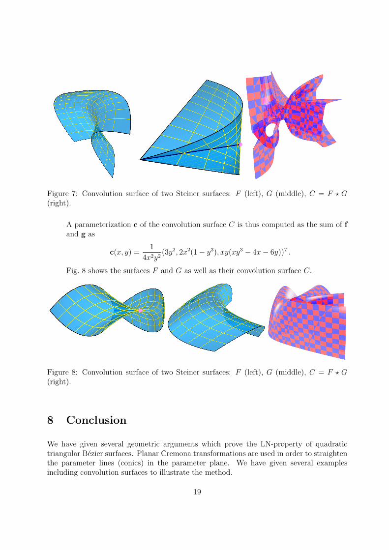
Figure 7: Convolution surface of two Steiner surfaces: F (left), G (middle), C = F ? G(right).

A parameterization c of the convolution surface C is thus computed as the sum of fand g as

c(x, y) =1

4x2y2(3y2, 2x2(1− y3), xy(xy3 − 4x− 6y))T .

Fig. 8 shows the surfaces F and G as well as their convolution surface C.

Figure 8: Convolution surface of two Steiner surfaces: F (left), G (middle), C = F ? G(right).

8 Conclusion

We have given several geometric arguments which prove the LN-property of quadratictriangular Bezier surfaces. Planar Cremona transformations are used in order to straightenthe parameter lines (conics) in the parameter plane. We have given several examplesincluding convolution surfaces to illustrate the method.

19

The LN-property in general can be characterized by the fact that the dual surface S is agraph of a rational function which is equivalent to the fact that the plane at infinity is ann− 1-fold tangent plane of surfaces S of class n.

Acknowledgments

This work has been funded in parts by the Austrian Science Fund FWF within the researchnetwork S92.

References

[1] Albrecht, G., 2002. The Veronese surface revisited, J. Geom. 73, 22-38.

[2] Apery, F., 1987. Models of the Real Projective Plane: Computer Graphics of Steinerand Boy Surfaces. Vieweg, Braunschweig.

[3] Bloomenthal, J. and Shoemake, K., 1991. Convolution Surfaces, Computer Graphics,Vol. 25, No. 4, 251–256.

[4] Coffmann, A., Schwartz, A.J., Stanton, C, 1995. The algebra and geometry of Steinerand other quadratically parameterizable surfaces, Comp. Aided Geom. Design 13 (1996),257–286.

[5] Degen, W.L.F., 1994. The Types of Triangular Bezier Surfaces, in: IMA Conferenceon the Mathematics of Surfaces, 153–170.

[6] Farin, G., Hoschek, J., and Kim, M.-S., 2002. Handbook of Computer Aided GeometricDesign, Elsevier.

[7] Fladt, K., 1933. Die Umkehrungen der ebenen quadratischen Cremona Transformatio-nen, J. reine u. angew. Math. 170, 64–68.

[8] Hoschek, J., Lasser, D., 1993. Fundamentals of Computer Aided Geometric Design. A.K. Peters, Wellesley, MA 1993.

[9] Juttler, B., 1998. Triangular Bezier surface patches with a linear normal vector field,in: The Mathematics of Surfaces VIII, Information Geometers, 431–446.

[10] Juttler, B. and Sampoli, M.L., 2000. Hermite interpolation by piecewise polynomialsurfaces with rational offsets, Comp. Aided Geom. Design 17, 361–385.

[11] Kummer, M., 1865. Uber die Flachen vierten Grades, auf welchen Scharen vonKegelschnitten liegen, J. reine u. angew. Math. 64, 66–96.

20

[12] Lavicka, M., Bastl B. 2006. Rational parameterized curves and surfaces with ra-tional convolutions. Algebraic Geometry and Geometric Modeling, Proc. of the conf.,Barcelona, 4.–7. Sept. 2006, 74–79.

[13] Lee, I.-K., Kim, M.-S. and Elber, G., 1998. Polynomial/Rational Approximation ofMinkowski Sum Boundary Curves, Graphical Models 60, No.2, 136–165.

[14] Lee, I.K., Kim, M.S. and Elber, G., 1998. The Minkowski Sum of 2D Curved Objects,Proceedings of Israel-Korea Bi-National Conference on New Themes in ComputerizedGeometrical Modeling, Feb.1998, Tel-Aviv University, 155–164.

[15] Meyer, W.F., 1903-1915. Spezielle algebraische Flachen. In: Enzyklopadie der Math-ematischen Wissenschaften, Teubner, Leipzig, III C 10, 1483–1490, 1647–1660.

[16] Muhlthaler, H. and Pottmann, H., 2003. Computing the Minkowski sum of ruledsurfaces, Graphical Models, 65, 369–384.

[17] Oeltze, S. and Preim, B., 2005, Visualization of Vasculature With Convolution Sur-faces: Method, Validation and Evaluation, IEEE Transactions on Medical Imaging,Vol. 24, No.4, 540–548.

[18] Peternell, M. and Manhart, F., 2003. The convolution of a paraboloid and aparametrized surface, Journal for Geometry and Graphics 7, 157-171.

[19] Peternell, M. and Pottmann, H., 1998. A Laguerre geometric approach to rationaloffsets, Computer Aided Geometric Design 15, 223–249.

[20] Pottmann, H., 1995. Rational curves and surfaces with rational offsets, ComputerAided Geometric Design 12, 175–192.

[21] Pottmann, H., 1995. Studying NURBS curves and surfaces with classical geometry,in: Mathematical Methods for Curves and Surfaces, eds: M. Dæhlen and T. Lyche andL. L. Schumaker, Vanderbilt University Press, 413–438.

[22] Peters, J., Reif, U., 1998. The 42 equivalence classes of quadratic surfaces in affinen-space, Comp. Aided Geom. Design 15, 459–473.

[23] Sampoli, M.L., Peternell, M. and Juttler, B., 2006. Exact parameterization of con-volution surfaces and rational surfaces with linear normals, Computer Aided GeometricDesign 23, 179–192.

[24] Schreier, O. and Sperner, E., 1961. Projective Geometry of n Dimensions, Chelsea,NY.

[25] Sederberg, T.W., Anderson, D.C., 1985. Steiner surface patches, IEEE Comp. Graph-ics & Applications 5, 23–36.

21

[26] Sherstyuk, A., 1999. Convolution Surfaces in Computer Graphics. PhD thesis, MonashUniv., Australia.

[27] Steiner, J., 1882. Gesammelte Werke II, Berlin, 723–724, 741–742.

[28] Wunderlich, W., 1968. Durch Schiebung erzeugbare Romerflachen, Sitzungsberichteder Osterreischen Akademie der Wissenschaften. 176, 473–497.

[29] Wunderlich, W., 1969. Kinematisch erzeugbare Romerflachen, J. reine u. angew. Math.236, 67–78.

[30] Wunderlich, W., 1962. Romerflachen mit ebenen Fallinien, Ann. di Mat. pura ed appl.57, 97–108.

22