Embed Size (px)
Citation preview
ECMWF flow dependent workshop, June 2007. Slide 1 of 14.
A regime-dependent balanced control variable based on
potential vorticity
Ross Bannister, Data Assimilation Research Centre, University of ReadingMike Cullen, Numerical Weather Prediction, Met Office
Funding: NERC and Met Office
ECMWF Workshop on Flow-dependent Aspects of Data Assimilation, 11-13th June 2007
ECMWF flow dependent workshop, June 2007. Slide 2 of 14.
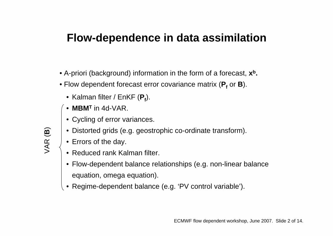
Flow-dependence in data assimilation
• A-priori (background) information in the form of a forecast, xb.• Flow dependent forecast error covariance matrix (Pf or B).
• Kalman filter / EnKF (Pf).• MBMT in 4d-VAR.• Cycling of error variances.• Distorted grids (e.g. geostrophic co-ordinate transform).• Errors of the day.• Reduced rank Kalman filter.• Flow-dependent balance relationships (e.g. non-linear balance
equation, omega equation).• Regime-dependent balance (e.g. ‘PV control variable’).
VA
R (B
)
ECMWF flow dependent workshop, June 2007. Slide 3 of 14.
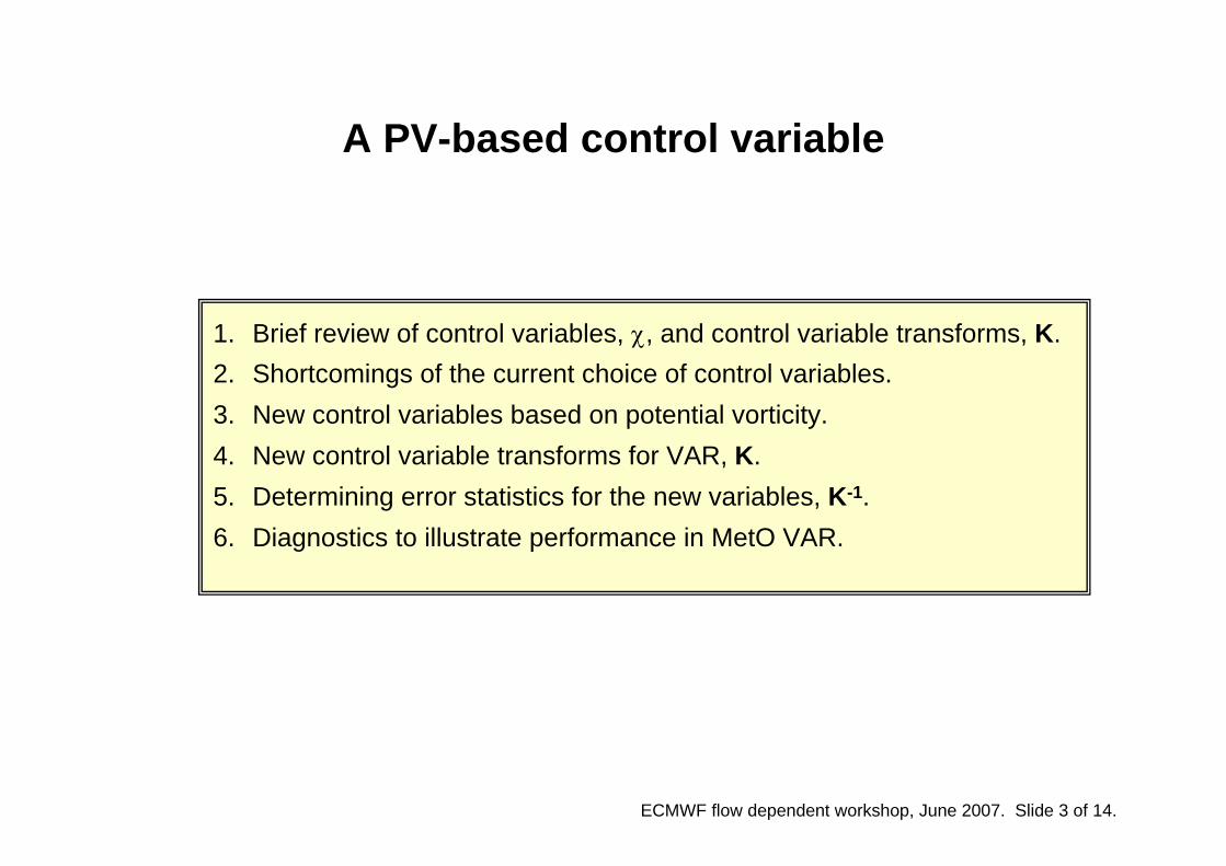
A PV-based control variable
1. Brief review of control variables, χ, and control variable transforms, K.2. Shortcomings of the current choice of control variables.3. New control variables based on potential vorticity.4. New control variable transforms for VAR, K.5. Determining error statistics for the new variables, K-1.6. Diagnostics to illustrate performance in MetO VAR.
ECMWF flow dependent workshop, June 2007. Slide 4 of 14.
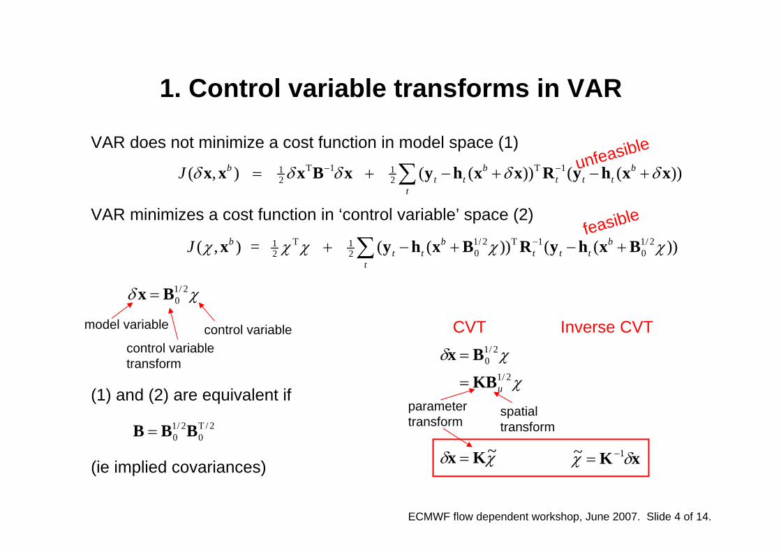
VAR does not minimize a cost function in model space (1)
VAR minimizes a cost function in ‘control variable’ space (2)
(1) and (2) are equivalent if
(ie implied covariances)
1. Control variable transforms in VAR
T 1 T 11 12 2( , ) ( ( )) ( ( ))b b b
t t t t tt
J δ δ δ δ δ− −= + − + − +∑x x x B x y h x x R y h x x
T 1/ 2 T 1 1/ 21 10 02 2( , ) = ( ( )) ( ( ))b b b
t t t t tt
J χ χ χ χ χ−+ − + − +∑x y h x B R y h x B
1/ 20δ χ=x B
1/ 2 T / 20 0=B B B
model variable
control variable transform
control variable
χδ
χ
χδ
~
2/1
2/10
Kx
KB
Bx
=
=
=
u
xK δχ 1~ −=
CVT Inverse CVT
parameter transform
spatial transform
unfeasible
feasible
ECMWF flow dependent workshop, June 2007. Slide 5 of 14.
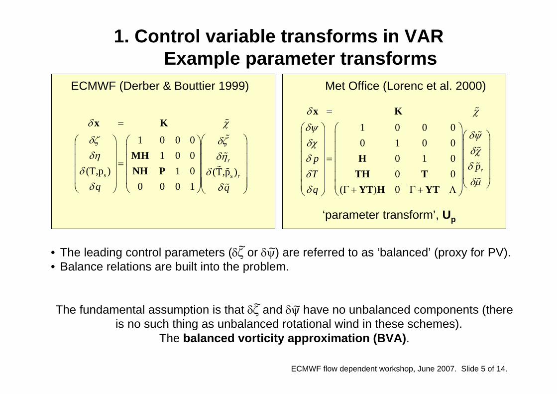
ECMWF (Derber & Bouttier 1999) Met Office (Lorenc et al. 2000)
‘parameter transform’, Up
1. Control variable transforms in VARExample parameter transforms
s s
1 0 0 01 0 0
(T,p ) 1 0 (T,p )0 0 0 1
r
r
q q
δ χ
δζ δζδη δη
δ δδ δ
=
⎛ ⎞⎛ ⎞ ⎛ ⎞⎜ ⎟⎜ ⎟ ⎜ ⎟⎜ ⎟⎜ ⎟ ⎜ ⎟= ⎜ ⎟⎜ ⎟ ⎜ ⎟⎜ ⎟⎜ ⎟ ⎜ ⎟⎜ ⎟⎝ ⎠ ⎝ ⎠⎝ ⎠
x K
MHNH P
• The leading control parameters (δζ or δψ) are referred to as ‘balanced’ (proxy for PV).• Balance relations are built into the problem.
The fundamental assumption is that δζ and δψ have no unbalanced components (there is no such thing as unbalanced rotational wind in these schemes).
The balanced vorticity approximation (BVA).
~
~
~
~
1 0 0 00 1 0 0
0 1 00 0
( ) 0
r
pp
Tq
δ χδψ
δψδχ
δχδ
δδ
δμδ
=
⎛ ⎞ ⎛ ⎞⎛ ⎞⎜ ⎟ ⎜ ⎟⎜ ⎟⎜ ⎟ ⎜ ⎟⎜ ⎟⎜ ⎟ ⎜ ⎟=⎜ ⎟⎜ ⎟ ⎜ ⎟⎜ ⎟⎜ ⎟ ⎜ ⎟⎝ ⎠⎜ ⎟ ⎜ ⎟Γ + Γ + Λ⎝ ⎠ ⎝ ⎠
x K
HTH TYT H YT
ECMWF flow dependent workshop, June 2007. Slide 6 of 14.
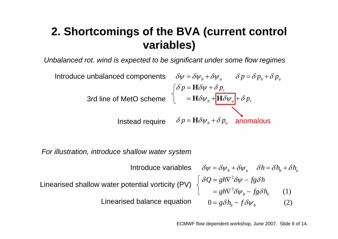
Unbalanced rot. wind is expected to be significant under some flow regimes
2. Shortcomings of the BVA (current control variables)
b u b u
r
b u r
b u
p p pp p
p
p p
δψ δψ δψ δ δ δδ δψ δ
δψ δψ δ
δ δψ δ
= + = += += + +
= +
HH H
H anomalous
Introduce unbalanced components
3rd line of MetO scheme
Instead require
2
2
(1)0 (2)
b u b u
b b
b b
h h h
Q gh fg hgh fg hg h f
δψ δψ δψ δ δ δ
δ δψ δ
δψ δδ δψ
= + = +
= ∇ −
= ∇ −= −
For illustration, introduce shallow water system
Introduce variables
Linearised shallow water potential vorticity (PV)
Linearised balance equation
ECMWF flow dependent workshop, June 2007. Slide 7 of 14.
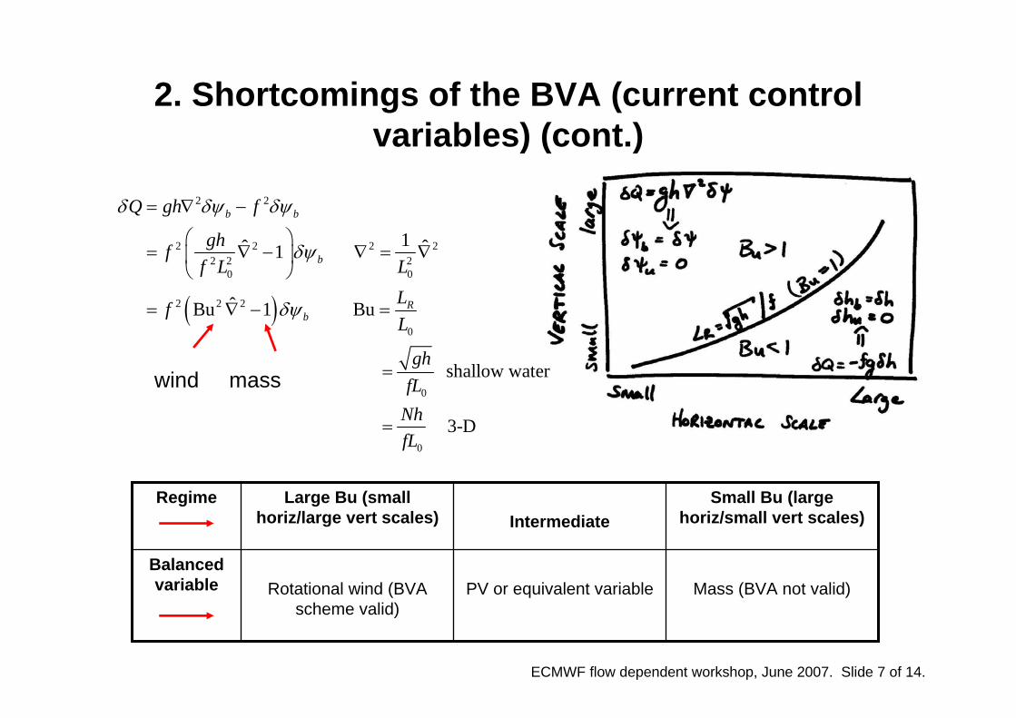
2. Shortcomings of the BVA (current control variables) (cont.)
( )
2 2
2 2 2 22 2 2
0 0
2 2 2
0
1ˆ ˆ1
ˆBu 1 Bu
b b
b
Rb
Q gh f
ghff L L
LfL
δ δψ δψ
δψ
δψ
= ∇ −
⎛ ⎞= ∇ − ∇ = ∇⎜ ⎟
⎝ ⎠
= ∇ − =
wind mass0
0
shallow water
3-D
ghfL
NhfL
=
=
PV or equivalent variable
Intermediate
Rotational wind (BVA scheme valid)
Large Bu (small horiz/large vert scales)
Mass (BVA not valid)Balanced variable
Small Bu (large horiz/small vert scales)
Regime
ECMWF flow dependent workshop, June 2007. Slide 8 of 14.
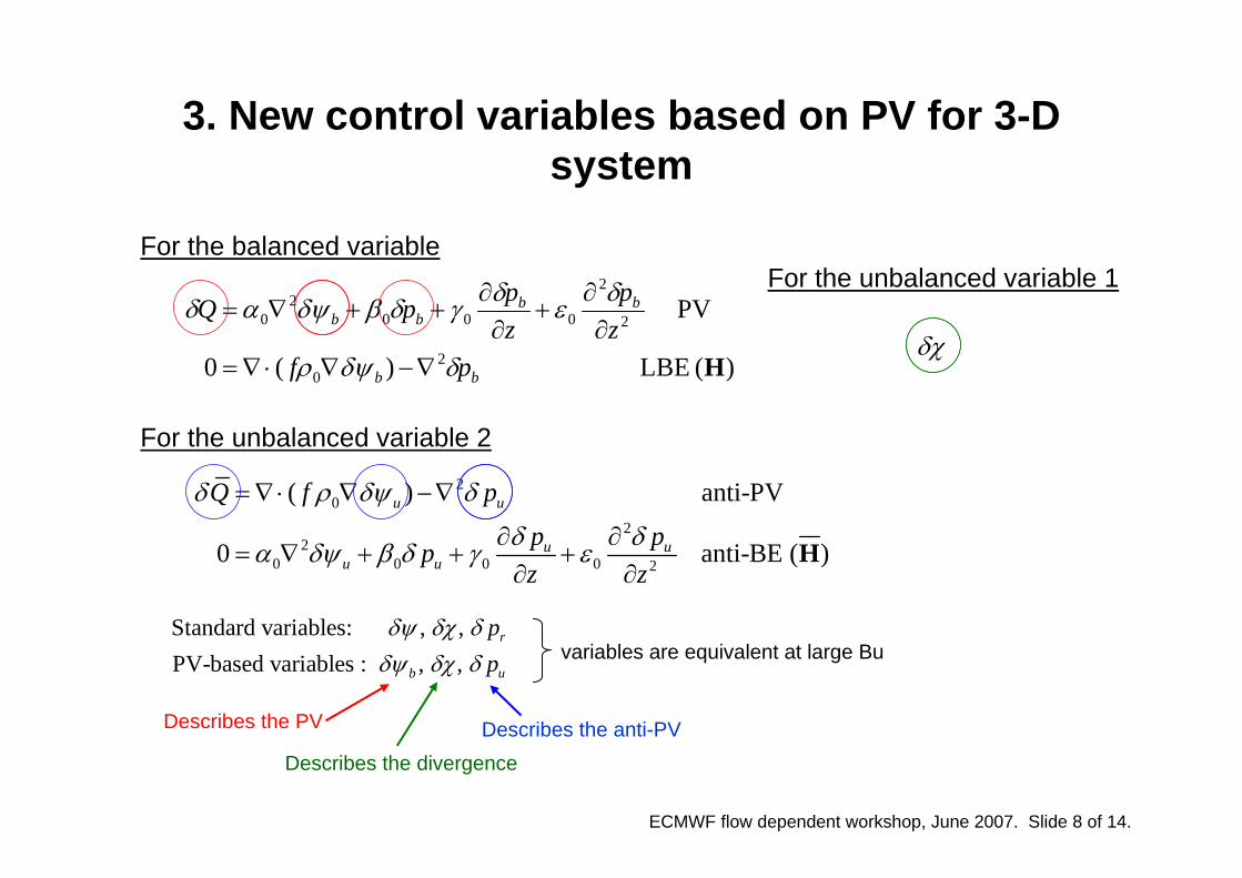
For the balanced variableFor the unbalanced variable 1
For the unbalanced variable 2
3. New control variables based on PV for 3-D system
)( LBE )(0
PV
20
2
2
0002
0
Hbb
bbbb
pfzp
zppQ
δδψρ
δεδγδβδψαδ
∇−∇⋅∇=∂∂
+∂∂
++∇=
20
22
0 0 0 0 2
( ) anti-PV
0 anti-BE ( )
u u
u uu u
Q f p
p ppz z
δ ρ δψ δ
δ δα δψ β δ γ ε
= ∇ ⋅ ∇ −∇
∂ ∂= ∇ + + +
∂ ∂H
δχ
Standard variables: , , PV-based variables : , ,
r
b u
pp
δψ δχ δδψ δχ δ
Describes the PV Describes the anti-PVDescribes the divergence
variables are equivalent at large Bu
ECMWF flow dependent workshop, June 2007. Slide 9 of 14.
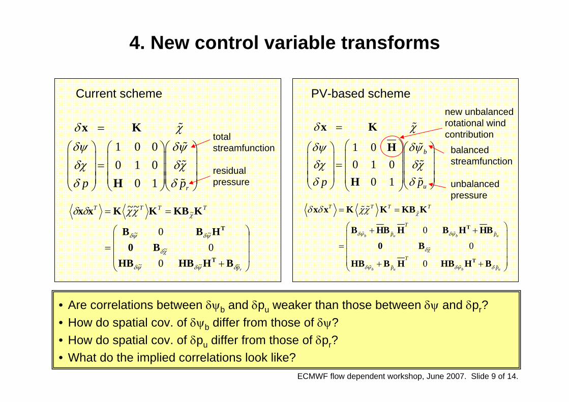
4. New control variable transforms
1 00 1 0
0 1
b
up p
δ χ
δψ δψδχ δχδ δ
=
⎛ ⎞⎛ ⎞ ⎛ ⎞⎜ ⎟⎜ ⎟ ⎜ ⎟= ⎜ ⎟⎜ ⎟ ⎜ ⎟
⎜ ⎟ ⎜ ⎟⎜ ⎟⎝ ⎠ ⎝ ⎠⎝ ⎠
x K
H
H
⎟⎟⎟
⎠
⎞
⎜⎜⎜
⎝
⎛
+=
==
rp
TTTT
~~~
~
~~
~
00
0
~~
δψδψδ
χδ
ψδψδ
χχχδδ
BHHBHBB0
HBB
KKBKKxx
T
T
1 0 00 1 0
0 1 rp p
δ χδψ δψδχ δχδ δ
=
⎛ ⎞ ⎛ ⎞⎛ ⎞⎜ ⎟ ⎜ ⎟⎜ ⎟=⎜ ⎟ ⎜ ⎟⎜ ⎟⎜ ⎟ ⎜ ⎟⎜ ⎟⎝ ⎠ ⎝ ⎠⎝ ⎠
x K
H
total streamfunction
residual pressure
balanced streamfunction
unbalanced pressure
new unbalanced rotational wind contribution
0
0
0
b u b u
b u b u
T T T T
T
p p
T
p p
χ
δψ δψ
δχ
δψ δψ δ
δ δ χχ= =
⎛ ⎞+ +⎜ ⎟⎜ ⎟=⎜ ⎟⎜ ⎟+ +⎝ ⎠
T
T
x x K K KB K
B HB H B H HB
0 B
HB B H HB H B
Current scheme PV-based scheme
• Are correlations between δψb and δpu weaker than those between δψ and δpr?• How do spatial cov. of δψb differ from those of δψ?• How do spatial cov. of δpu differ from those of δpr?• What do the implied correlations look like?
ECMWF flow dependent workshop, June 2007. Slide 10 of 14.
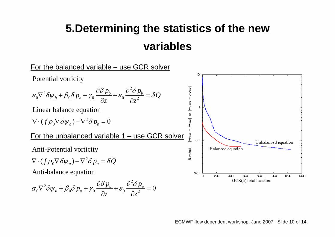
5.Determining the statistics of the new variables
For the balanced variable – use GCR solver
For the unbalanced variable 1 – use GCR solver
22
0 0 0 0 2
20
Potential vorticity
Linear balance equation( ) 0
b bb b
b b
p pp Qz z
f p
δ δε δψ β δ γ ε δ
ρ δψ δ
∂ ∂∇ + + + =
∂ ∂
∇ ⋅ ∇ −∇ =
20
22
0 0 0 0 2
Anti-Potential vorticity( )
Anti-balance equation
0
u u
u uu u
f p Q
p ppz z
ρ δψ δ δ
δ δα δψ β δ γ ε
∇ ⋅ ∇ −∇ =
∂ ∂∇ + + + =
∂ ∂
ECMWF flow dependent workshop, June 2007. Slide 11 of 14.
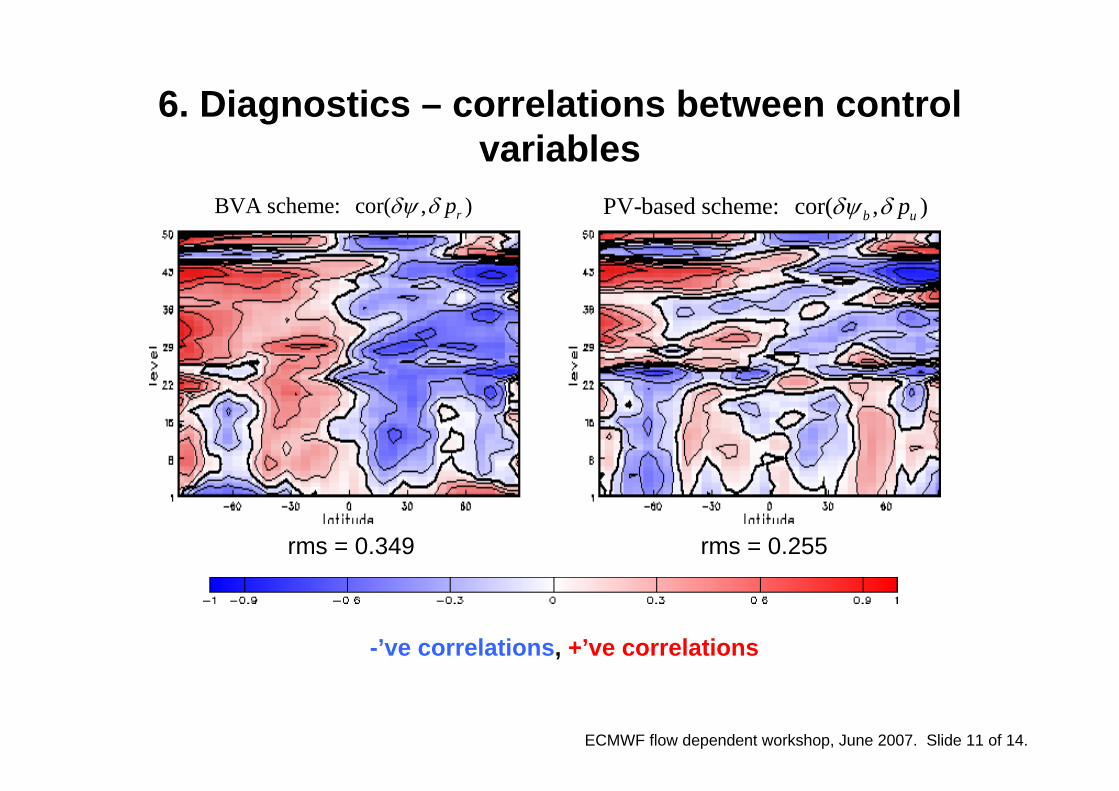
6. Diagnostics – correlations between control variables
BVA scheme: cor( , )rpδψ δ
-’ve correlations, +’ve correlations
PV-based scheme: cor( , )b upδψ δ
rms = 0.349 rms = 0.255
ECMWF flow dependent workshop, June 2007. Slide 12 of 14.
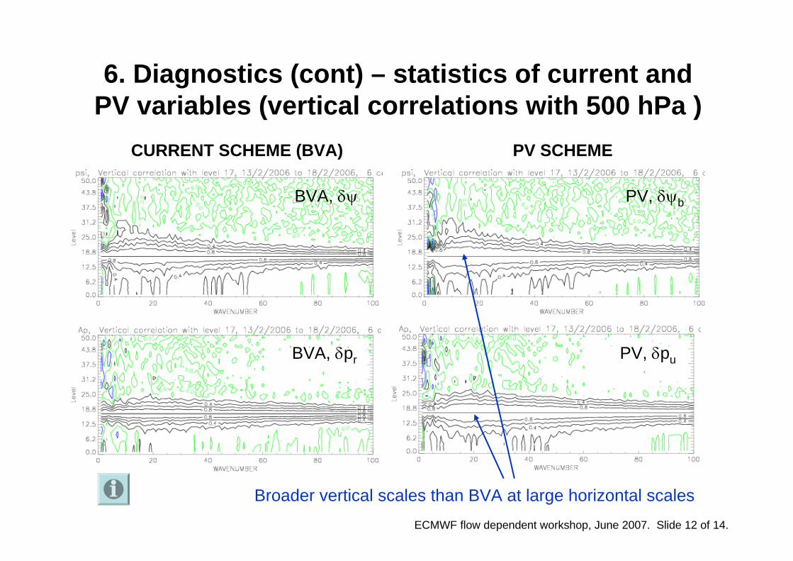
6. Diagnostics (cont) – statistics of current and PV variables (vertical correlations with 500 hPa )
CURRENT SCHEME (BVA) PV SCHEME
BVA, δψ
BVA, δpr
PV, δψb
PV, δpu
Broader vertical scales than BVA at large horizontal scales
ECMWF flow dependent workshop, June 2007. Slide 13 of 14.
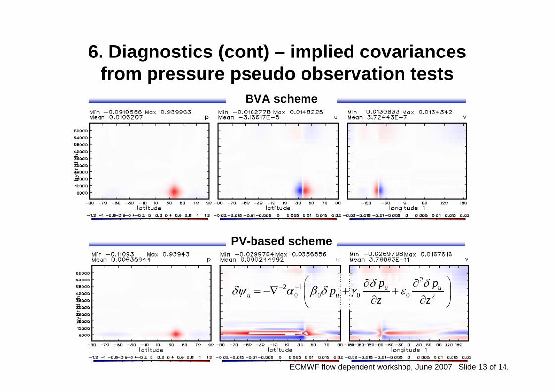
6. Diagnostics (cont) – implied covariancesfrom pressure pseudo observation tests
BVA scheme
PV-based scheme
22 1
0 0 0 0 2u u
u up ppz z
δ δδψ α β δ γ ε− − ⎛ ⎞∂ ∂= −∇ + +⎜ ⎟∂ ∂⎝ ⎠
ECMWF flow dependent workshop, June 2007. Slide 14 of 14.
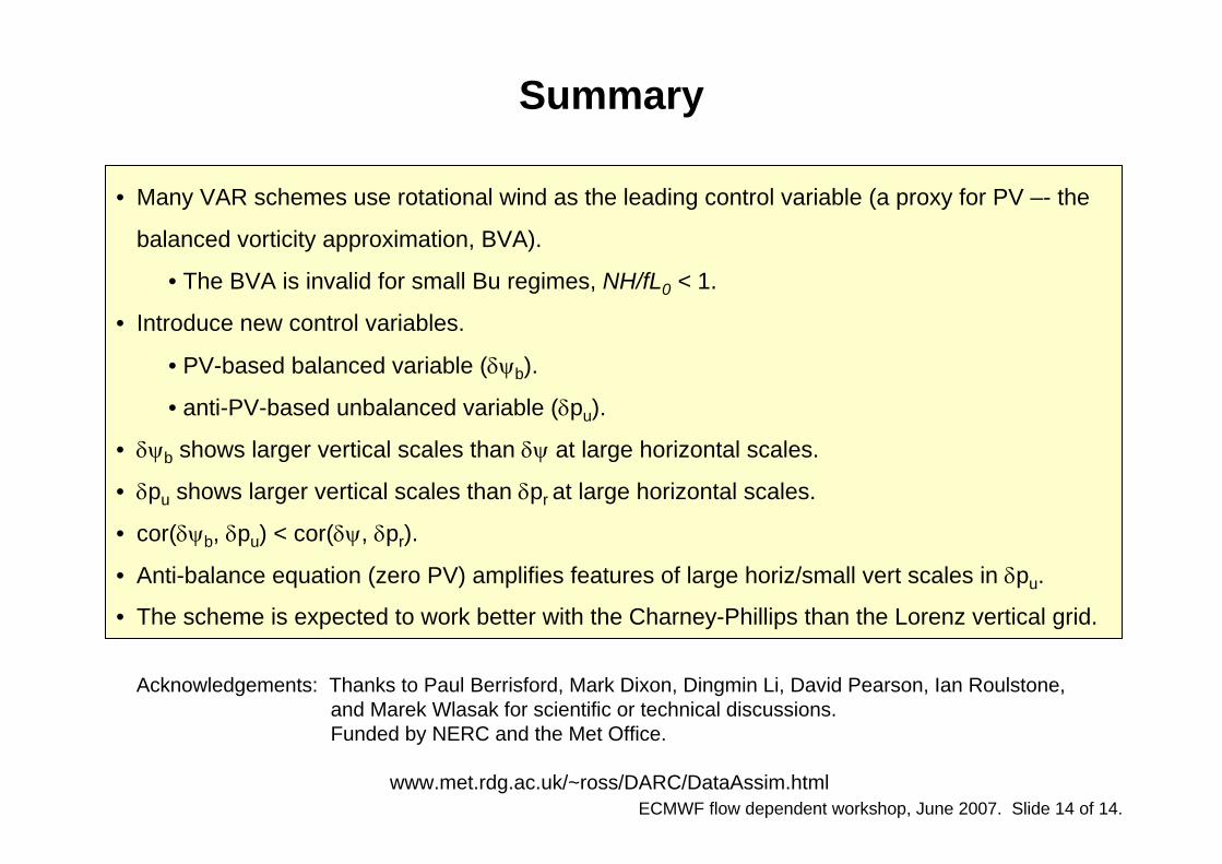
Summary
Acknowledgements: Thanks to Paul Berrisford, Mark Dixon, Dingmin Li, David Pearson, Ian Roulstone, and Marek Wlasak for scientific or technical discussions.Funded by NERC and the Met Office.
www.met.rdg.ac.uk/~ross/DARC/DataAssim.html
• Many VAR schemes use rotational wind as the leading control variable (a proxy for PV –- the
balanced vorticity approximation, BVA).
• The BVA is invalid for small Bu regimes, NH/fL0 < 1.
• Introduce new control variables.
• PV-based balanced variable (δψb).
• anti-PV-based unbalanced variable (δpu).
• δψb shows larger vertical scales than δψ at large horizontal scales.
• δpu shows larger vertical scales than δpr at large horizontal scales.
• cor(δψb, δpu) < cor(δψ, δpr).
• Anti-balance equation (zero PV) amplifies features of large horiz/small vert scales in δpu.
• The scheme is expected to work better with the Charney-Phillips than the Lorenz vertical grid.
ECMWF flow dependent workshop, June 2007. Slide 15 of 14.
End
ECMWF flow dependent workshop, June 2007. Slide 16 of 14.
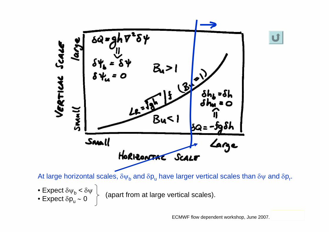
At large horizontal scales, δψb and δpu have larger vertical scales than δψ and δpr.
• Expect δψb < δψ• Expect δpu ∼ 0 (apart from at large vertical scales).
ECMWF flow dependent workshop, June 2007. Slide 17 of 14.
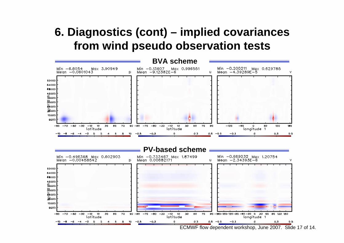
6. Diagnostics (cont) – implied covariancesfrom wind pseudo observation tests
BVA scheme
PV-based scheme
ECMWF flow dependent workshop, June 2007. Slide 18 of 14.
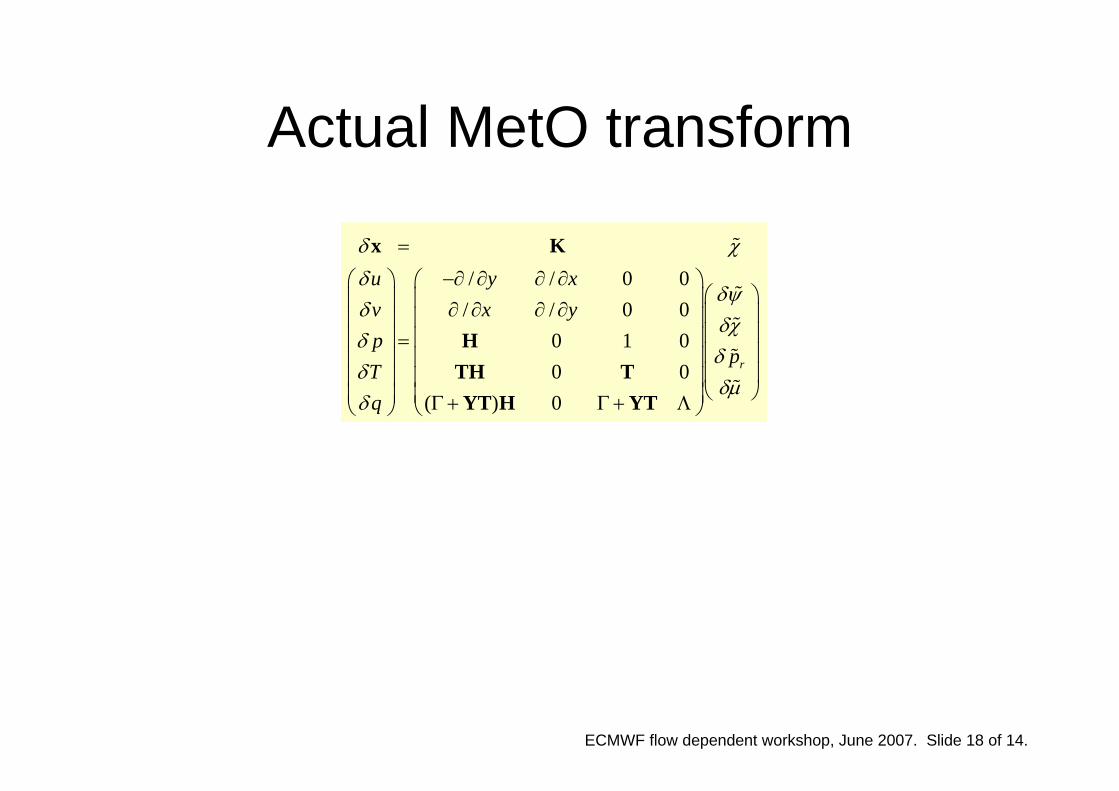
Actual MetO transform
/ / 0 0
/ / 0 00 1 00 0
( ) 0
r
u y xv x yp
pTq
δ χδ
δψδ
δχδ
δδ
δμδ
=
−∂ ∂ ∂ ∂⎛ ⎞ ⎛ ⎞⎛ ⎞⎜ ⎟ ⎜ ⎟∂ ∂ ∂ ∂ ⎜ ⎟⎜ ⎟ ⎜ ⎟⎜ ⎟⎜ ⎟ ⎜ ⎟=⎜ ⎟⎜ ⎟ ⎜ ⎟⎜ ⎟⎜ ⎟ ⎜ ⎟⎝ ⎠⎜ ⎟ ⎜ ⎟Γ + Γ + Λ⎝ ⎠ ⎝ ⎠
x K
HTH TYT H YT


![Theoretical study of orientation-dependent multiphoton ... · atoms and molecules [12]. And the exploration of the attosec-ond electronic dynamics in the strong-field regime has](https://img.pdfslide.net/doc/110x75/5f528ecf2c008e4f16726dd5/theoretical-study-of-orientation-dependent-multiphoton-atoms-and-molecules-12.jpg)