Embed Size (px)
Citation preview
A Rehabilitation Manual for Australian Streams
VOLUME 2
Ian D. Rutherfurd, Kathryn Jerie and Nicholas Marsh
Cooperative Research Centre for Catchment Hydrology
Land and Water Resources Research and Development Corporation
2000

Published by: Land and Water Resources Research and Cooperative Research CentreDevelopment Corporation for Catchment HydrologyGPO Box 2182 Department of Civil EngineeringCanberra ACT 2601 Monash UniversityTelephone: (02) 6257 3379 Clayton VIC 3168Facsimile: (02) 6257 3420 Telephone: (03) 9905 2704Email: <[email protected]> Facsimile: (03) 9905 5033WebSite: <www.lwrrdc.gov.au>
© LWRRDC and CRCCH
Disclaimer: This manual has been prepared from existing technical material, from research and development studies and from specialist input by researchers, practitioners and stream managers. The material presented cannot fully represent conditions that may be encountered for any particular project. LWRRDC and CRCCH have endeavoured to verify that the methods and recommendations contained are appropriate. No warranty or guarantee, express or implied, except to the extent required by statute, is made as to the accuracy, reliability orsuitability of the methods or recommendations, including any financial and legal information.
The information, including guidelines and recommendations, contained in this Manual is made available by the authors to assist public knowledge and discussion and to help rehabilitate Australian streams. The Manual is not intended to be a code or industry standard. Whilst it is provided in good faith, LWRRDC and CRCCH accept no liability in respect of any loss or damage caused by reliance on that information. Users should make their own enquiries, including obtaining professional technical, legal and financial advice,before relying on any information and form their own views as to whether the information is applicable to their circumstances. Where technical information has been prepared by or contributed by authors external to LWRRDC and CRCCH, readers should contact the author/s or undertake other appropriate enquiries before making use of that information.
The adoption of any guidelines or recommendations in the manual will not necessarily ensure compliance with any statutory obligations, the suitability or stability of any stream structure or treatment, enhanced environmental performance or avoidance of environmental harm or nuisance.
Publication data: ‘A Rehabilitation Manual for Australian Streams Volume 2’
Authors: Ian D. Rutherfurd, Kathryn Jerie and Nicholas MarshCooperative Research Centre for Catchment HydrologyDepartment of Geography and Environmental StudiesUniversity of MelbourneVIC 3010Telephone: (03) 9344 7123Facsimile: (03) 9344 4972Email: [email protected]
ISBN 0 642 76029 2 (volume 2/2)ISBN 0 642 76030 6 (set of 2 volumes)
Design by: Arawang Communication Group, Canberra
December 1999 Web versionMarch 2000 Printed version
This manual was first published (in colour) on the World Wide Web, where it can be accessed at <www.rivers.gov.au>. For economy and convenience, that pagination of the Web version has beenretained here.

Volume 2 Contents 3
TABLE OF CONTENTSFeedback Sheet 9Preamble 11Figure Acknowledgements 12
Part 1: Common Stream Problems 13
Preserving Valuable Reaches 14
Identifying valuable reaches 15
Preserving a reach in good condition 16
A summary and ranking of stream degradation issues 181 Implications 20
Geomorphic Problems 21
Geomorphic problems:an introduction 22
Chains-of-ponds:description and rehabilitation 231 Description 23
2 Threats to chains-of-ponds 24
3 Change if no action 25
4 Potential for rehabilitation 25
5 Rehabilitation techniques 25
Gullies 261 Introduction 26
2 Description 26
3 Changes if no action 27
4 Potential for rehabilitation 27
Valley floor incised streams (also, incised channelised streams) 291 Description 29
2 Changes if no action 29
3 Ecological significance 30
4 Appropriate tools for management 30
Larger over-widened streams 311 Description 31
2 Changes if no action 32
3 Appropriate tools for management 32
Typical small, enlarged rural streams 331 Introduction 33
2 Ecological significance 33
3 Appropriate tools for management 33

Volume 2 Contents 4
Sediment slugs 341 Introduction 34
2 Appropriate tools for management 36
Water Quality Problems 37
Water quality:an introduction 381 Common attributes of water quality problems 38
Turbidity and fine sediment 401 Introduction 40
2 Biological impacts of turbidity and fine sediment 40
3 Other water quality issues 43
4 How do you recognise turbidity and fine sediment? 43
5 At what stage does turbidity and fine sediment become a problem? 44
6 Possible treatments for turbidity 45
Nutrient enrichment 471 Introduction 47
2 Biological impacts of nutrient enrichment 47
3 How do you recognise nutrient enrichment? 48
4 What nutrient concentration is a problem? 50
5 Possible solutions/treatments for nutrient enrichment 53
Dissolved oxygen concentration 541 Introduction 54
2 Biological impacts of low dissolved oxygen 55
3 How do you recognise low dissolved oxygen? 55
4 At what stage does low oxygen concentration become a problem? 56
5 Possible solutions/treatments for low dissolved oxygen 56
High and low temperatures 571 Introduction 57
2 Biological impacts of changes in temperature 57
3 How do you recognise changes in temperature? 58
4 At what stage do changes in temperature become a problem? 58
5 Possible solutions/treatments for changes in temperature 59
Salinity 601 Introduction 60
2 Biological impacts of salinity 60
3 How do you recognise salinity? 62
4 At what stage does salinity become a problem? 63
5 Possible solutions/treatments for salinity 64
Toxicants 651 Introduction 65
2 Biological impacts of toxicants 65
3 How do you recognise the presence of toxicants? 65
4 At what stage do toxicants become a problem? 66
5 Possible solutions/treatments for toxicants 66

Volume 2 Contents 5
Other Biological Problems 67
Other biological problems:an introduction 68
Barriers to fish migration 691 Introduction 69
2 Effects of blocking migrations 69
3 The extent of the problem 70
4 Identifying barriers to fish passage 70
5 Techniques for creating fish passage 71
Large woody debris 721 Introduction 72
2 Biological and physical effects of LWD 72
3 The physical effects of large woody debris on streams 74
4 Managing large woody debris 74
Stock management 751 Introduction 75
2 The effect of stock on stream rehabilitation 75
3 Managing stock access 76
Rehabilitation for platypuses 771 Introduction 77
2 Biology of the platypus 77
3 Do you already have platypuses? 78
4 Habitat requirements 79
5 Water quality requirements 80
6 Rehabilitation tips 81
7 Further reading 81
Rehabilitation for frogs 821 Introduction 82
2 Do you already have frogs? 82
3 Habitat requirements 82
4 Food and hunting 83
5 Flow regulation 83
6 Life cycles 83
7 Water quality 84
8 Rehabilitation tips 84
Part 2: Planning Tools 85
Natural Channel Design 86
Catchment review:developing a catchment perspective and describing your stream 871 An introduction to catchment review 87
2 Dividing the stream into manageable units (Task 1 of Step 3) 87
3 Developing a template of the stream condition (Task 2 of Step 3) 91
4 Describing the condition of the reaches (Task 3 of Step 3) 92

Volume 2 Contents 6
5 Determining the interactions between reaches 101
6 Determining the key problems in the reach 102
Designing a more natural stream 1071 Setting realistic objectives 107
2 Selecting a procedure to design the stream template 109
3 Using historical reconstruction to develop a template 112
4 Using a reference reach to develop a template 114
Empirical approaches to designing a naturally stable channel 1221 An introduction to the empirical approach to channel design 123
2 Selecting a design discharge 124
3 Hydraulic geometry equations and regime equations 135
4 Channel design details 139
5 A worked hypothetical application of the regime approach 141
6 Limitations of the empirical model approach 142
The channel evolution approach to rehabilitation design 143
Predicting the scour produced when you put things into streams 1451 What happens when you put something into a stream? 145
2 Increasing pool habitat 146
3 Substrate variability and scour holes 146
4 General hydraulic effects of instream structures 148
How changing the channel can affect flooding 1531 Open-channel flow: general concepts and useful formulae 153
2 Predicting backwater effects 159
Evaluation Tools 179
Evaluation 1801 Fundamentals of evaluation design 180
2 Planning the evaluation of a rehabilitation project 185
3 Evaluation case studies 209
Miscellaneous Planning Tools 216
Why stakeholders may not support your plan 217
Setting priorities for stream rehabilitation 2201 Where do I start?—the reach priority shuffle 220
2 Which problem do I fix first? 224
3 Prioritisation case studies 226
Legislative and administrative constraints 2311 Queensland stream management 231
2 New South Wales stream management 233
3 Western Australian stream management 234
4 Victorian stream management 236
5 South Australian stream management 239
6 Tasmanian stream management 241

Volume 2 Contents 7
Benefit–cost analysis of stream rehabilitation projects 2431 The difficulty of applying BCA 243
2 How to value non-market goods 244
The geographic information system (GIS) as a stream rehabilitation tool 2501 What is a GIS and how much does it cost to set up? 250
2 Are the analysis tools of a full-blown GIS really helpful in planning a rehabilitation project? 250
3 Analysis of GIS information 251
4 Data transfer 251
5 Is the effort and cost of GIS worth it? What are the benefits and costs? 252
Some costs of stream rehabilitation activities 2531 The costs of stream management works 253
2 Additional costs of stream rehabilitation works 255
Bibliography of some technical information available in Australia 2561 A bibliography of fact sheets 256
2 Abbreviations and contact details 262
Part 3: Intervention Tools 264
Introduction to the intervention tools section 2651 Intervention in the channel 265
2 Intervention in the riparian zone 266
Intervention in the Channel 267
Full-width structures 2681 Tried and true full-width structures 268
2 Design considerations for full-width structures 268
3 Design variations for rock full-width structures 269
4 Experimental full-width structures 274
Partial-width bank erosion control structures 2781 Tried and true partial-width structures 278
2 Experimental partial-width structures 280
Longitudinal bank protection 2901 Incorporating vegetation into bank protection 290
Bed replenishment 298
Reinstating cut-off meanders 3001 Introduction 300
2 Where is re-meandering inappropriate? 301
3 Secondary effects of re-meandering 302
Fish cover 303

Volume 2 Contents 8
Boulders 3041 Installing boulders 304
Overcoming barriers to fish passage 306
Management of large woody debris 3131 Re-introduction techniques for instream large woody debris 313
2 Other effects of reinstating large woody debris 321
Sand and gravel extraction as a rehabilitation tool 3261 Erosion effects of extraction 327
2 Secondary effects of extraction 328
3 Using extraction to manage sediment slugs 328
4 How do I know that the bed is aggrading? 329
5 Where to extract from? 330
6 How much to extract? 331
7 Standard rules of any extraction operation 332
8 Using extraction to fund stream rehabilitation 332
9 Examples of rehabilitation extraction 333
Intervention in the Riparian Zone 335
Vegetation management 3361 The role of vegetation in stabilising stream banks 336
2 In-channel vegetation: macrophytes and emergent plants 341
3 Some tips for revegetation 343
4 Direct-seeding methods 345
Streams infested by exotic weeds 3491 Managing exotic vegetation 349
2 Management of exotic weeds 350
Willow-infested streams 3511 Introduction 351
2 The effects of willows on streams 351
3 Managing willows 354
Managing stock access to streams 3601 Fencing the riparian corridor 360
2 Alternative stock watering 361
Glossary 364
Bibliography 383

A Rehabilitation Manual for Australian Streams, Volume 2
We need your feedback!
We want to know what you think of this manual: what parts of it you find most useful; what parts are least useful; what might be added; how the presentation might be improved. On the matter of presentation, please note that the manual was first published (in colour) on the World Wide Web, where can be accessed at <www.rivers.gov.au>. For economy and convenience, the pagination of the Web version has been retained here.
We also want to know about your experiences in stream rehabilitation, so we can develop a data bank of case studies in stream work in Australia. Please use the space on the other side of this form to tell us what you have done or are doing.
Sharing your experiences will help. The stream rehabilitation industry is in its infancy, but it will grow and mature. We hope that this manual will foster this and will itself evolve as we learn from each other about the business of stream rehabilitation. By sharing, evaluating and recording the successes and failures of our stream rehabilitation efforts we will gain the confidence needed to begin roll back the many decades of degradation that our streams have suffered.
Please complete this two-page questionnaire (we suggest you use a photocopy), providing as much information as you can. Return the completed form to: Dr Siwan Lovett, Program Coordinator, River Restoration & Riparian Lands, LWRRDC, GPO Box 2182, Canberra ACT 2601; Fax: (02) 6257 3420; email: <public@ lwrrdc.gov.au>.
QUESTIONNAIRE
The parts of the manual which I found most useful were: ....................................................................................................
........................................................................................................................................................................................
The parts of the manual which I found least useful were: ....................................................................................................
........................................................................................................................................................................................
General comments on content: ..........................................................................................................................................
........................................................................................................................................................................................
An updated version should contain more or new information on: ........................................................................................
........................................................................................................................................................................................
I found the information in the manual was well-organised and easy to navigate (please tick appropriate box):
Yes
No
General comments on presentation: ..................................................................................................................................
........................................................................................................................................................................................
... over
9

The presentation of an updated version could be improved by: ...........................................................................................
........................................................................................................................................................................................
I would purchase a copy of a new edition of the manual if it were available as a:
book
CD-ROM (please tick preference)
I have looked at the World Wide Web version of the manual:
Yes
No
If ‘yes’, please comment on its usefulness or otherwise: ......................................................................................................
........................................................................................................................................................................................
I AM OR HAVE BEEN INVOLVED IN STREAM REHABILITATION OR RELATED ACTIVITIES (PLEASE TICK APPROPRIATE BOX)
Yes
No
If ‘Yes’ please provide, in the box below, a brief account of the aims and outcomes of the work in which you are/were involved.
Name: ..........................................................................Affiliation: .................................................................................
Postal address: .................................................................................................................................................................
........................................................................................................................................................................................
Fax: ..............................................................................Email: .......................................................................................
Please return the completed form to: Dr Siwan Lovett, Program Coordinator, River Restoration and Riparian Lands, LWRRDC, GPO Box 2182, Canberra ACT 2601; Fax: (02) 6257 3420; email: <public@ lwrrdc.gov.au>.
10

Volume 2 Preamble 1 1
PREAMBLEThis document forms the second part of A Rehabilitation
Manual for Australian Streams. The manual is designed to
help professional managers who are attempting to return
some of the biological and physical values of Australia’s
streams.Volume 1 of the manual provides some
rehabilitation concepts, and a summary of a rehabilitation
planning procedure.Volume 2 provides more detailed
information about the tools that can be used for
rehabilitation.Volume 2 is divided into three sections:
1. Common stream problems
2. Planning tools
3. Intervention tools.
Our expectation is that managers would occasionally dip
into Volume 2 if they need more detail than is provided in
Volume 1. There are many cross-references from Volume 1
to the more detailed information in Volume 2. Please have
a look through the table of contents to see what is included
in Volume 2.
Please note that both volumes are available from the Land
and Water Resources Research and Development
Corporation website (www.rivers.gov.au).
It is important to emphasise that this is not a catchment or
stream management manual. There are many reasons to
intervene in streams and catchments that are not related to
rehabilitation of the natural stream values. Thus, the
manual will only touch on issues such as erosion control,
water supply, flooding, and the sociology of management,
in so far as they affect rehabilitation.
Also, this is not an engineering design manual. We provide
some concepts, and guidance, but where detailed design
information is required we will refer you to a better source.
This manual was only possible with the contribution of
many managers and researchers across Australia. These
contributions are acknowledged at the front of Volume 1
and often as footnotes to the text. We also acknowledge the
generous support and vision of the Land and Water
Resources Research and Development Corporation, and
the Cooperative Research Centre for Catchment Hydrology
that has brought this manual to fruition.
Please note:a comprehensive glossary of terms is provided at the end of
this manual.

A Rehabilitation Manual for Australian Streams 1 2
FIGURE ACKNOWLEDGMENTS
We wish to thank the following publishers for permission to reproduce copyright material in the A Rehabilitation Manual for
Australian Streams,Volume 2.
Publisher Figure number Source etc.
EPA Victoria Figure 15, Figure 1 from Tiller and Newall (1995). EPA copyright
Common Stream Problems material. Reproduced by permission of the Environmental
Protection Authority (Victoria). First published by the
Environmental Protection Authority, GPO Box 4395QQ,
Melbourne,Victoria 3001.
These documents are not an official copy of EPA copyright
material and the Environmental Protection Authority
(Victoria) and the State of Victoria accept no responsibility
for their accuracy.
Wildland Hydrology Figures 32, 35 and 40, Figures 8–17, 8–21 and 8–24 from Rosgen (1996).
Intervention Tools
Centre for Environmental Figures 19 and 21, Figures 10 and 12 from Stewardson et al. (1997).
Applied Hydrology Intervention Tools
Blackwell Science Figures 27–30, Figures 11.4, 11.6, 11.7 and 11.9 from Underwood (1996).
Planning Tools, Evaluation
Newbury Hydraulics Figures 6 and 7, Figures 4–16, 4–18 and 4–19 from Newbury and Gaboury
Intervention Tools (1993).
American Water Figure 31, Intervention Tools Figure 2 from Shields et al. (1998).
Resources Association
Center for Computational Figures 5 and 6, Common Figures 1 and 2 from Rutherfurd et al. (1997).
Hydroscience and Stream Problems
Engineering
Land Victoria, Department Figure 38, Intervention Tools Aerial photograph Latrobe Valley PHD 1908 Run 4
of Natural Resources 19/2/1987.
and Environment

PART 1:COMMON STREAM
PROBLEMS

PRESERVING VALUABLE REACHES
Please note:The following pages are a cursory discussion of this important
subject.
Dr Helen Dunn from the School of Geography and
Environmental Studies at the University of Tasmania is
presently (mid 1999) completing a LWRRDC project
investigating the identification and protection of rivers with
high ecological value.The results of this investigation will be
incorporated into this section when they become available.
They will also be available on http://www.rivers.gov.au
• Identifying valuable reaches
• Preserving a reach in good condition
• A summary and ranking of stream degradationissues

Volume 2 Common Stream Problems: Preserving valuable reaches 1 5
A reach can have high conservation value for two reasons.
1. It supports a rare species of plant or animal, or a rare
community type.
2. The reach is in excellent overall condition. Such reaches
are often chosen as reference or template reaches.
Briefly, the presence of rare species can be checked by
contacting your State Herbarium and/or Department of
Environment. These organisations should have records of
the distribution of rare species of plants and animals,
respectively. Also, if there have been biological surveys of
your stream, you can check species lists against lists of
known rare species. It is possible to search the Australian
Heritage Commission’s Register of the National Estate to
check for sites of national significance that may be
relevant to your stream (Skull et al., 1996).
IDENTIFYING VALUABLE REACHES
Volume 2 Common Stream Problems: Preserving valuable reaches 1 6
1.1. Introduction
In this manual we have emphasised the importance of
preserving the natural assets of streams that remain in
good condition. But how do you do this? We will assume
here that the asset is a discrete reach of stream that may be
valuable in its own right, or that supports animals or
plants that are rare. We discuss three approaches to
preserving such assets. These are: physical protection;
planning controls; and identifying threats.
1.2. Physical protection
In some cases it may be necessary to physically protect the
reach of stream from damage. This is most commonly
done by fencing the stream (see Managing stock access to
streams, in Intervention in the riparian zone, this Volume).
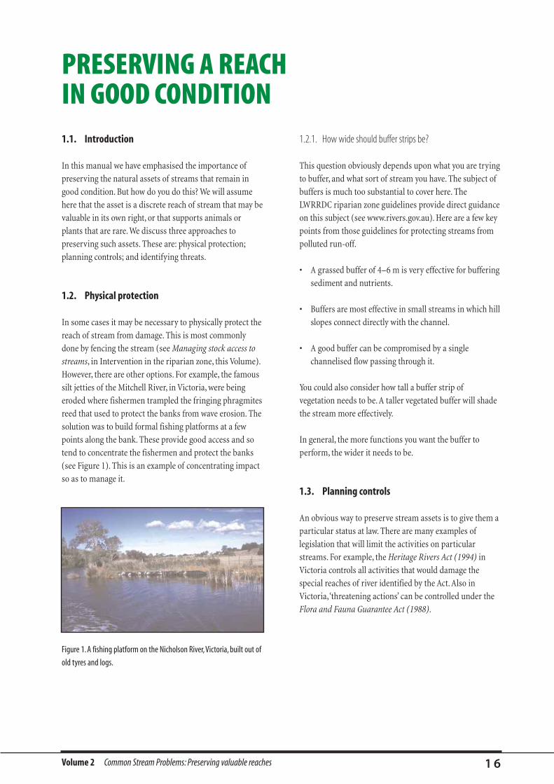
However, there are other options. For example, the famous
silt jetties of the Mitchell River, in Victoria, were being
eroded where fishermen trampled the fringing phragmites
reed that used to protect the banks from wave erosion. The
solution was to build formal fishing platforms at a few
points along the bank. These provide good access and so
tend to concentrate the fishermen and protect the banks
(see Figure 1). This is an example of concentrating impact
so as to manage it.
Figure 1. A fishing platform on the Nicholson River,Victoria, built out of
old tyres and logs.
1.2.1. How wide should buffer strips be?
This question obviously depends upon what you are trying
to buffer, and what sort of stream you have. The subject of
buffers is much too substantial to cover here. The
LWRRDC riparian zone guidelines provide direct guidance
on this subject (see www.rivers.gov.au). Here are a few key
points from those guidelines for protecting streams from
polluted run-off.
• A grassed buffer of 4–6 m is very effective for buffering
sediment and nutrients.
• Buffers are most effective in small streams in which hill
slopes connect directly with the channel.
• A good buffer can be compromised by a single
channelised flow passing through it.
You could also consider how tall a buffer strip of
vegetation needs to be. A taller vegetated buffer will shade
the stream more effectively.
In general, the more functions you want the buffer to
perform, the wider it needs to be.
1.3. Planning controls
An obvious way to preserve stream assets is to give them a
particular status at law. There are many examples of
legislation that will limit the activities on particular
streams. For example, the Heritage Rivers Act (1994) in
Victoria controls all activities that would damage the
special reaches of river identified by the Act. Also in
Victoria,‘threatening actions’ can be controlled under the
Flora and Fauna Guarantee Act (1988).
PRESERVING A REACH IN GOOD CONDITION
Volume 2 Common Stream Problems: Preserving valuable reaches 1 7
Stream frontages can be an area of overlapping
jurisdiction. It is important that a reach is flagged as being
important in any branches of government that could have
some jurisdiction over the land. For example, different
departments in Queensland manage the estuarine and
freshwater parts of the stream system. One planning
agency may be officially sanctioning damage to the natural
assets of a stream reach, while another department is
trying to preserve them.
It is often useful to publicise the special values of a stream
reach. Around Victoria you often see the ‘Land for Wildlife’
signs that identify areas as being of special habitat value. It
can be effective to let adjacent landholders know that a
reach of stream is important, and get them on-side in
managing the asset. Statistics can be helpful here: “This is
part of the 5% of this stream that is still in good condition.
Congratulations on preserving such an important piece of
stream! Can we talk about how this reach could be
managed?”
1.4. Identify and eliminate threats to the targetreach
An obvious thing that one can do to protect reaches is to
identify and eliminate existing and developing problems. A
process for identifying, and prioritising, threats to high
value reaches is built into Step 5 of the Stream
rehabilitation procedure,Volume 1. This procedure looks
for threats to the target reach from:
• upstream (sediment, water quality, floods, major
changes of course);
• downstream (erosion knickpoints, exotic fish, boats);
and
• the riparian zone (stock access, fishermen, weeds,
clearing, excess light).
Here is an obvious example of solving the damaging
problem. The banks of the Gordon River have been eroded
up to 10 m by waves from cruise boats (Bradbury et al.,
1995). This river is in a World Heritage Area and has
obvious high value. The solution was to dramatically
reduce boat speed.

Volume 2 Common Stream Problems: Preserving valuable reaches 1 8
Possibly the most common underlying vision that drives
stream rehabilitation is to improve the health of stream, or
to make the stream more biologically similar to an
undisturbed pre-European condition. Because it is the
plants and animals that we wish to encourage, it would be
useful to know their perspective on stream problems. Any
organism will have numerous requirements of its
environment, and there are many processes which will
degrade these requirements. Tables 1–3 list the main
issues which contribute to the degradation or restoration
of macroinvertebrates, fish and floodplains, and also
indicate the likely importance of each issue.
Table 1. Restoration and degradation issues important to
macroinvertebrates in the Murray–Darling Basin. From Koehn et al.
(1997b).
Restoration/degradation issue Importance (high – low) comments
Riparian vegetation Very high – not so much for itself, but most other degradation issues are
affected by this.
Sedimentation High – very widespread, changes fundamental habitat characteristics,
essentially irreversible once having occurred (ie. needs natural cleaning).
Water flow, volume, seasonality Probably Low, (except for zero flow, and some low flows – see Temperature
and Dissolved oxygen concentration, below); flow for fish probably more important.
Water quality – temperature High in places, especially below low release dams, small unshaded streams,
possibly extremely low flows.
Water quality – nutrients Possibly Medium, but definitely High in places, below sewage treatment plants,
dairy, piggery outlets, some factories (dealt with by EPA).
Water quality – toxicants High in places, below licensed discharges. Accidental pulse spills may be dramatic,
but may not be important in the long term.
Water quality – pH, dissolved oxygen, salinity Medium – streams with high salinity are High. In-stream habitat,
bed structure High – particularly in rock streams subject to sedimentation.
In-stream habitat, including snags and fringing vegetation Medium – not a major problem in upland sections, more important in lowland
streams where snags and banks are possibly the only productive habitat.
Predation by exotic fish Low – they probably can’t eat enough.
Competition by exotic invertebrates Overall Low, but High in specific places.
In 1996, at the 1st Stream Management Conference, held at
Merrijig near Mount Buller,Victoria, a group of conference
delegates stood next to the beautiful Delatite River watching
fish ecologists electrofish in the stream.The Delatite River
appears to be a pristine mountain stream with perfect riparian
vegetation, good water quality and original in stream
structures.The delegates were looking forward to seeing a
‘natural’ range of native fish species from an undisturbed
stream. Instead, they were shocked to find all that was caught
was trout and more trout.These exotic fish appear to have
completely displaced the native fish in the stream.This
demonstrates that the viability of organisms can be
threatened in numerous ways.
A SUMMARY AND RANKING OF STREAM DEGRADATION ISSUES
Volume 2 Common Stream Problems: Preserving valuable reaches 1 9
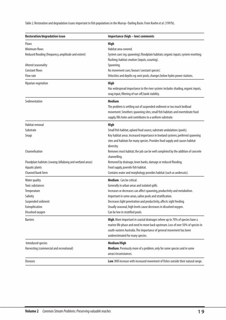
Restoration/degradation issue Importance (high – low) comments
Flows High
Minimum flows Habitat area covered.
Reduced flooding (frequency, amplitude and extent) System cues (eg. spawning); floodplain habitats; organic inputs; system resetting;
flushing; habitat creation (inputs, scouring).
Altered seasonality Spawning.
Constant flows No movement cues; favours ‘constant species’.
Flow rate Velocities and depths eg. weir pools, changes below hydro power stations.
Riparian vegetation High
Has widespread importance to the river system: includes shading, organic inputs,
snag input, filtering of run-off, bank stability.
Sedimentation Medium
The problem is settling out of suspended sediment or too much bedload
movement. Smothers spawning sites, small fish habitats and invertebrate food
supply, fills holes and contributes to a uniform substrate.
Habitat removal High
Substrate Small fish habitat, upland food source, substrate undulations (pools).
Snags Key habitat areas. Increased importance in lowland systems; preferred spawning
sites and habitats for many species. Provides food supply and causes habitat
diversity.
Channelisation Removes most habitat; the job can be well completed by the addition of concrete
channelling.
Floodplain habitats (swamp, billabong and wetland areas) Removed by drainage, levee banks, damage or reduced flooding.
Aquatic plants Food supply, juvenile fish habitat.
Channel/bank form Contains water and morphology provides habitat (such as undercuts).
Water quality Medium. Can be critical.
Toxic substances Generally in urban areas and isolated spills.
Temperature Increases or decreases can affect spawning, productivity and metabolism.
Salinity Important in some areas, saline pools and stratification.
Suspended sediment Decreases light penetration and productivity, affects sight feeding.
Eutrophication Usually seasonal, high levels cause decreases in dissolved oxygen.
Dissolved oxygen Can be low in stratified pools.
Barriers High. More important in coastal drainages where up to 70% of species have a
marine life phase and need to move back upstream. Loss of over 50% of species in
south-eastern Australia.The importance of general movement has been
underestimated for many species.
Introduced species Medium/High
Harvesting (commercial and recreational) Medium. Previously more of a problem, only for some species and in some
areas/circumstances.
Diseases Low.Will increase with increased movement of fishes outside their natural range.
Table 2. Restoration and degradation issues important to fish populations in the Murray–Darling Basin. From Koehn et al. (1997b).
Volume 2 Common Stream Problems: Preserving valuable reaches 2 0
Every species has a long list of requirements of its
environment, many of which are essential for survival.
Unfortunately, for many species, these requirements are
basically unknown, which makes it difficult to design a
rehabilitation program to suit one animal or plant. Even
for those species where some environmental requirements
are known, we seldom, if ever, have the complete picture.
Basing a rehabilitation project on such incomplete
information risks damaging one important aspect of
habitat while trying to fix another. For this reason, we
recommend a more basic approach of working out
rehabilitation goals by copying the characteristics of a
stream which does manage to support a diverse aquatic
community. Ideally, these characteristics would be based
on the original condition of the stream in question.
Alternatively, you could use a ‘template’ reach—a stream
section which currently supports the organisms you wish
to encourage. When ‘copying’ either the original condition,
or a template reach, you should examine:
• the structure and form of the channel bed, including
adjacent benches and banks;
• the riparian zone, including flow connection with the
floodplain;
• free passage between different habitat areas;
• the flow regime, including variability over many years;
• the water quality; and
• the natural complement of indigenous animals and
plants.
In the absence of evidence to the contrary, stream
rehabilitators should see these six characteristics of the
stream as their target for management. As the example on
page 15 demonstrates, it is important to consider the role
that all of these play in the condition of any stream.
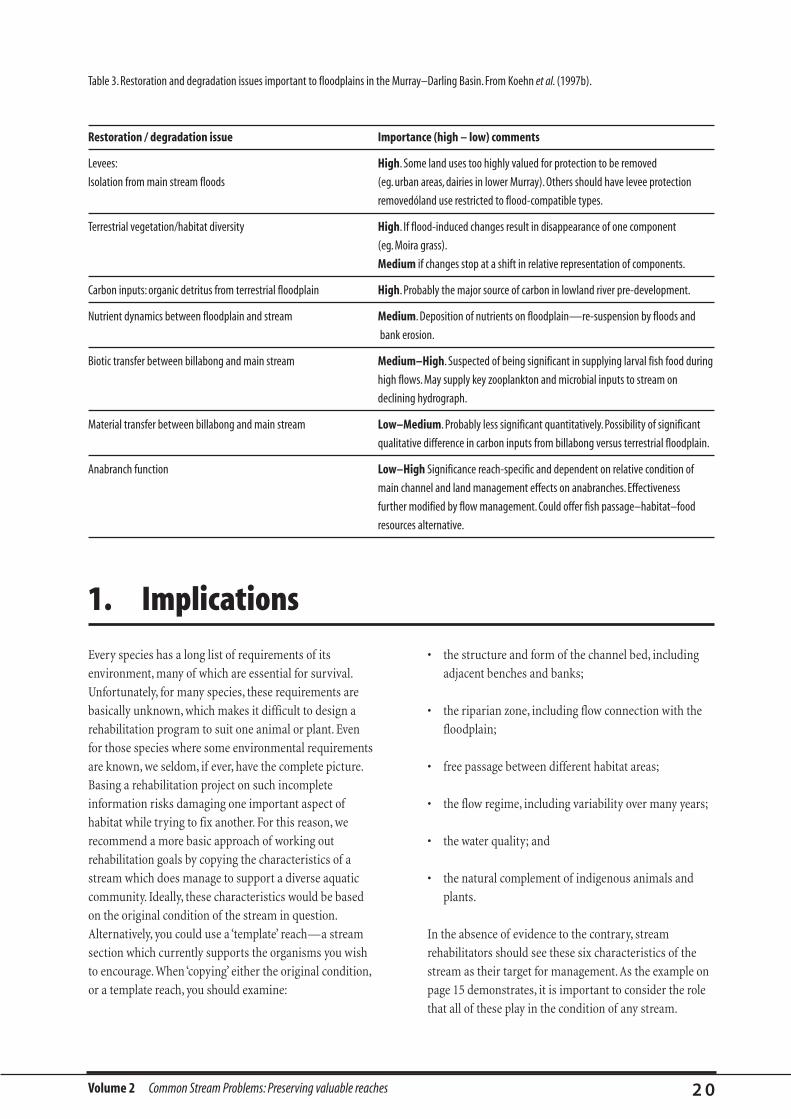
Restoration / degradation issue Importance (high – low) comments
Levees: High. Some land uses too highly valued for protection to be removed
Isolation from main stream floods (eg. urban areas, dairies in lower Murray). Others should have levee protection
removedóland use restricted to flood-compatible types.
Terrestrial vegetation/habitat diversity High. If flood-induced changes result in disappearance of one component
(eg. Moira grass).
Medium if changes stop at a shift in relative representation of components.
Carbon inputs: organic detritus from terrestrial floodplain High. Probably the major source of carbon in lowland river pre-development.
Nutrient dynamics between floodplain and stream Medium. Deposition of nutrients on floodplain—re-suspension by floods and
bank erosion.
Biotic transfer between billabong and main stream Medium–High. Suspected of being significant in supplying larval fish food during
high flows. May supply key zooplankton and microbial inputs to stream on
declining hydrograph.
Material transfer between billabong and main stream Low–Medium. Probably less significant quantitatively. Possibility of significant
qualitative difference in carbon inputs from billabong versus terrestrial floodplain.
Anabranch function Low–High Significance reach-specific and dependent on relative condition of
main channel and land management effects on anabranches. Effectiveness
further modified by flow management. Could offer fish passage–habitat–food
resources alternative.
1. Implications
Table 3. Restoration and degradation issues important to floodplains in the Murray–Darling Basin. From Koehn et al. (1997b).

GEOMORPHICPROBLEMS
• Geomorphic problems: an introduction
• Chains-of-ponds: description and rehabilitation
• Gullies
• Valley floor incised streams (also, incisedchannelised streams)
• Larger over-widened streams
• Typical small, enlarged rural streams
• Sediment slugs

Volume 2 Common Stream Problems: Geomorphic problems 2 2
Many rehabilitation projects in streams focus on the
geomorphic condition of the channel and floodplain. This
might be because treating the geomorphic problems
(whether erosion or sedimentation) is sometimes the best
way to treat water quality problems (such as turbidity),
and is often a prerequisite for successful rehabilitation of
the stream ecology. Some geomorphic problems can be
classified into similar types that require similar treatment.
Further discussion on these geomorphic problems can be
found in Rutherfurd (in press). Here we briefly discuss:
• chains-of-ponds;
• gullies;
• valley-floor incised streams (including channelised
streams);
• larger over-widened streams;
• small, enlarged rural channels; and
• sediment slugs.
GEOMORPHIC PROBLEMS:AN INTRODUCTION

Volume 2 Common Stream Problems: Geomorphic problems 2 3
Much international work in stream rehabilitation assumes
that the natural state of small streams was to have pools
and riffles. As a result, returning pools and riffles is the
focus of much rehabilitation design. By contrast, at first
settlement, numerous streams throughout south-eastern
Australia (including South Australia and Tasmania) had a
quite different morphology consisting of chains-of-ponds,
or the related swampy meadows (Prosser, 1991).
Swampy meadows are poorly drained, confined valley
floors in which sediments and organic matter gradually
build-up (Prosser et al., 1994). Chains-of-ponds consist of
deep, permanent pools, separated by bars of sediment
stabilised with vegetation (Eyles, 1977b). They are
typically found on smaller streams, with non-perennial
flow regimes. There is no regularity to the spacing of the
ponds down the drainage line. Unlike pool-and-riffle
sequences, the ponds are not always associated with
stream bends, although there will generally be a pool
located where a tributary enters the main channel.
Chains-of-ponds appear to be more common in Australia
than elsewhere, perhaps due to climatic variability
producing infrequent high flows that form ponds,
interspersed with long periods of low stream flow that
allow vegetation to become established between the ponds
(eg. Figure 2). Before and during European settlement,
chains-of-ponds were reported to exist in many streams,
both coastal and inland, from Western Australia to
Queensland (Eyles, 1977b; Gaydon et al., 1996).
Two types were categorised by Bannerman in Herron
(1993) according to the dominant process that forms the
ponds:
1. Scour chains-of-ponds are formed where sheet flow
over a gradual slope of varying erodibility leads to
depressions that are deepened by scour. This form is
more likely to occur on duplex soils. In this situation, a
resistant topsoil stabilised by vegetation overlays a
dispersible clay. If a scour hole penetrates through a
weak point in the surface layer, the clay gradually
erodes by dispersion.Yabbies may contribute to this
erosion. The ponds grow in size until an equilibrium is
established between erosion and sedimentation in
reeds at the pond edges. The impermeability of the clay
maintains water in the pool during long dry periods.
This form generally exists on alluvial plains, above the
limit of a well-defined channel. Scour ponds have been
known to remain in equilibrium for 140 years (Eyles,
1977b).
2. Depositional chains-of-ponds on channelised reaches
form by the deposition of fixed bars which block the
channel, producing long pools. This is different to a
pool-and-riffle sequence by virtue of the irregularity in
pond spacing and the large amount of vegetation
CHAINS-OF-PONDS:DESCRIPTION AND REHABILITATIONWritten with the assistance of Scott Wilkinson and Barry Starr
1. Description
Figure 2. A remnant chain-of-ponds in the Goulburn River catchment,
Victoria.
Volume 2 Common Stream Problems: Geomorphic problems 2 4
1.1. Ecological significance
Chains-of-ponds were often the only source of stock water
for early pastoralists, but equally they provided permanent
water for wildlife. Chains-of-ponds, and related swampy
valley-fills, are of great ecological significance because
they were the natural state of so many of our small and
medium-sized streams. Unfortunately, we know little
about their original physical state, let alone of the flora and
fauna that occupied them.
Chains-of-ponds can be destroyed when channel incision
cuts through the inter-pond bars from downstream (Eyles,
1977a; Herron, 1993; see Figure 3). Incision of swampy
meadows has similarly been related to flow concentration
and damage to valley-floor vegetation (Prosser and Slade,
1994). The incision in chains-of-ponds can start when the
upstream end of a pond becomes unstable, and develops
into a gully head that cuts through the bar to the next
pond, thus draining it. Such a process can be contributed
to by:
• digging drains through inter-pond bars;
• damaging the vegetation in the flow-line between the
ponds, by stock grazing, fire, increased salinity; or
• increased stream flows (or higher peaks) caused by
catchment clearing or gullying upstream.
These changes have been associated with increases in
stream erosion capacity and sediment transport. The
erosion power of a stream determines the morphology of
the chain-of-ponds. As stream erosion capacity increases,
the most likely morphology progresses from: scour
depressions; scour ponds; extended ponds gullying at the
head; discontinuous gully; continuous gully containing
fixed bar ponds; permanently flowing stream (Eyles,
1977a). A threat of a different kind to chains-of-ponds is a
large sediment supply from upstream, as a result of poor
catchment management or channel erosion. This can fill
the ponds with sediment.
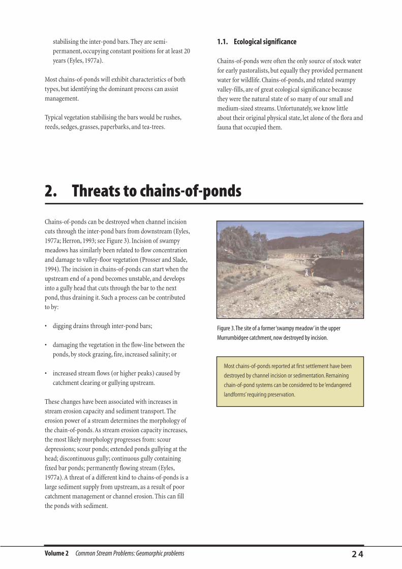
Figure 3.The site of a former ‘swampy meadow’ in the upper
Murrumbidgee catchment, now destroyed by incision.
2. Threats to chains-of-ponds
Most chains-of-ponds reported at first settlement have been
destroyed by channel incision or sedimentation. Remaining
chain-of-pond systems can be considered to be ‘endangered
landforms’ requiring preservation.
stabilising the inter-pond bars. They are semi-
permanent, occupying constant positions for at least 20
years (Eyles, 1977a).
Most chains-of-ponds will exhibit characteristics of both
types, but identifying the dominant process can assist
management.
Typical vegetation stabilising the bars would be rushes,
reeds, sedges, grasses, paperbarks, and tea-trees.

Volume 2 Common Stream Problems: Geomorphic problems 2 5
A stable chain-of-ponds relies on the equilibrium between
many variables including stream flow, vegetation health,
and sediment supply and transport. Chains-of-ponds are
commonly threatened by channel incision progressing
from downstream, or sedimentation from upstream. If
there is an active gully head below a chain-of-ponds, or a
large amount of mobile sediment in the channel upstream,
or the vegetation is damaged in some way, the morphology
will be significantly altered.
Once channelisation has occurred, natural reformation of
a scour chain-of-ponds morphology would be unlikely, or
at best a long-term proposition. An integral feature of
scour chains-of-ponds is a non-channelised stream. A
scour chain-of-ponds may naturally reform if the channel
had widened through meandering enough to provide
effectively non-channelised flow and allow vegetation to
become established on a flat bed.
3. Change if no action
There is limited potential for returning chains-of-ponds to
their original state. The incised streams that have replaced
the chains-of-ponds have high stream powers, and provide
a hostile environment for revegetation (see Gullies, below).
As a general principle, it is easier to protect chains-of-
ponds from damage than it is to recreate them, although
rehabilitation experience to date is limited. There follows a
list of some tools for both stabilisation and restoration of
the chain-of-ponds morphology (Table 4).
Some groups are already using chains-of-ponds as a model
for stream rehabilitation. River engineers have had some
success in north-east Victoria, and in Gippsland, in
Table 4. Some strategies and tools to rehabilitate chains-of-ponds for various objectives.
Rehabilitation objectives Strategies Techniques and tools
To prevent a gully from progressing Stabilise the gully head. • Rock chute at gully head.
upstream through a chain-of-ponds. • Exclude stock from gully head and inter-pond bars.
• Pasture improvement and revegetation in the catchment to reduce run-off.
To protect a chain-of-ponds from a Manage sediment movement. • Sediment monitoring and management to prevent ponds infilling
sediment slug. with sand.
To recreate a depositional style Create stable pools and bars. • Low earthen and rock weirs, well-vegetated with
chain-of-ponds in a channelised stream. appropriate species to prevent erosion (eg. plant reeds on low weirs).
• Vegetate and fence stream verges.
• Install artificial sediment trap or use an existing pond sacrificially.
• Controlled sediment extraction from sediment traps, or the
channel upstream of the chain-of-ponds.
encouraging the development of a chain-of-ponds. They
stabilised the bed of gullies with rock-chutes, but, to create
a pool, set the crest of the chute slightly higher than
normal. The upstream end of the pool was then densely
vegetated. Phragmites reeds were scooped-up from nearby
wetlands (where they are abundant) by an excavator,
placed in a truck, and were then dumped into the
upstream end, and around the margins of, the pool. The
phragmites then began to trap sediment.
5. Rehabilitation techniques
4. Potential for rehabilitation
Although we cannot recreate the unique conditions that
developed the ponds, we can use the chains-of-ponds as a
model for rehabilitating incised streams.
Volume 2 Common Stream Problems: Geomorphic problems 2 6
Gullies are a subset of ‘incised streams’, usually referring to
streams that are reasonably ‘new’, that is, there was
probably no defined channel before settlement, and the
gullies represent deepening and extension of the drainage
network (eg. see Figure 4). About 5% of New South Wales
is affected by ‘severe’ gullying (Soil Conservation Service of
NSW, 1989). The fullest review of eastern Australian
gullying is provided by Prosser and Winchester (1996).
2.1. Original state (physical and ecological)
Gullies have developed in almost every environment
across Australia. There was often no defined channel at
first settlement, just a swale or swampy area (often called a
swampy meadow). In many cases the areas that have
gullied can be defined as ‘sediment accumulation zones’
that gradually build-up with sediment and then naturally
strip that sediment out by gullying every few thousand
years. The difference with human-induced gullying is that
it has occurred within a century right across the country,
and often to greater depths than the natural gullying.
There are many triggers for gullying, but they usually
included a combination of clearing of vegetation from the
catchments, concentration of flow by vehicle and animal
tracks, drainage or plough-lines, and periods of intense
rainfall. Catchment clearing alone is usually insufficient to
trigger gullying.
2.2. Present condition
Gullies rapidly cut a box-shaped channel with vertical
walls, with further development continuing at a negative
exponential rate (Figures 5 and 6). This means that they
will erode at a much slower rate in the future than they
have in the past for the same set of rainfall events. The
gully proceeds up the drainage network as a set of erosion
heads (knickpoints). Once incised, the gully increases the
drainage of groundwater into the trench and erosion is
increasingly driven by seepage processes.
The large volume of sediment eroded from gullies is often
deposited in ‘flood-outs’ further downstream as the depth
of the gully decreases.
2.3. Ecological significance
Many gullies began as chains-of-ponds, or similar ill-
defined channels. There are few examples of this stream
type left, so rehabilitating examples is desirable.
Gullies often have low ecological diversity because they
combine highly variable flow with high velocity flow. They
also tend to have unstable bed and banks, providing poor
habitat.
One of the major ecological reasons to manage gullies is that
they are often the major source of sediment, particularly high
turbidity and associated phosphorus, to the rest of the stream
network (Caitcheon, 1990; Wallbrink et al., 1996). Controlling
erosion in gullies may be justified for this reason alone.
GULLIES
1. Introduction
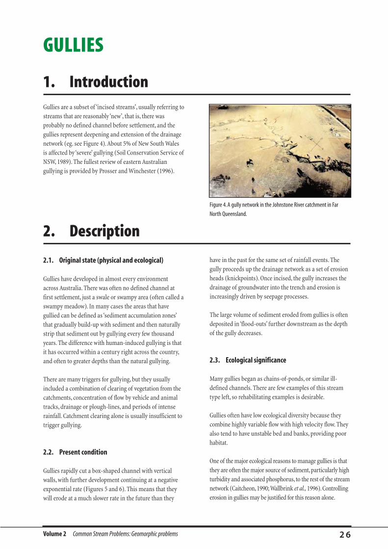
Figure 4. A gully network in the Johnstone River catchment in Far
North Queensland.
2. Description
Volume 2 Common Stream Problems: Geomorphic problems 2 7
Gullies usually develop at a negative exponential rate. This
means that, given the same run-off conditions, gullies will
almost always erode at a much lower rate in any successive
period (Figures 5 and 6). Thus, research has shown that
the numerous gullies that developed in the dry years of the
1940s in south-eastern Australia have, in general, mostly
stabilised (Prosser and Winchester, 1996). Remember that
raw banks and an ugly appearance do not necessarily
imply a rapid erosion rate.
Gullies will eventually stabilise, and the beds will
revegetate, but it will take several decades. There are
usually three reasons why gullies are slow to heal: (1)
because of the high flow velocities that occur in the bed of
the gully; (2) because of the seepage erosion driven by the
depth of the gully; and (3) because water and soil quality
is often poor in the gully floor (eg. saline in many areas),
hampering plant growth.
3. Changes if no action
Time since initiation (years)
0 2 4 6 8 10
800
600
400
200
0
Gul
ly le
ngth
(m
)
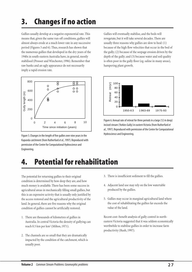
Figure 5. Changes in the length of five gullies over nine years in the
Kapunda catchment (from Rutherfurd et al., 1997). Reproduced with
permission of the Centre for Computational Hydroscience and
Engineering.
0
20
40
60
80
100
1950-6 3 1 963-69 19 75-93R
etr
ea
t (m
/yr)
Figure 6. Annual rate of retreat for three periods in a large (12 m deep)
incised stream (Yorkies Gully) in eastern Victoria (from Rutherfurd et
al., 1997). Reproduced with permission of the Centre for Computational
Hydroscience and Engineering.
The potential for returning gullies to their original
condition is determined by how deep they are, and how
much money is available. There has been some success in
agricultural areas in mechanically filling small gullies, but
this is an expensive activity that is usually only justified by
the access restored and the agricultural productivity of the
land. In general, there are five reasons why the original
condition of gullies cannot be artificially restored.
1. There are thousands of kilometres of gullies in
Australia. In central Victoria the density of gullying can
reach 0.5 km per km2 (Milton, 1971).
2. The channels are so small that they are dramatically
impacted by the condition of the catchment, which is
usually poor.
3. There is insufficient sediment to fill the gullies.
4. Adjacent land use may rely on the low watertable
produced by the gullies.
5. Gullies may occur in marginal agricultural land where
the cost of rehabilitating the gullies far exceeds the
value of the land.
Recent cost–benefit analysis of gully control in north-
eastern Victoria suggested that it was seldom economically
worthwhile to stabilise gullies in order to increase farm
productivity (Rush, 1997).
4. Potential for rehabilitation
Volume 2 Common Stream Problems: Geomorphic problems 2 8
4.1. Appropriate tools for rehabilitation
The management principles for stabilising gullies are:
• aim to accelerate the natural process of recovery;
• always stabilise the bed before the bank (see Full width
structures, in Intervention in the channel, this Volume);
• encourage invasion of the channel bed by vegetation to
accelerate stability; and
• wherever possible divert high flows out of the channel,
but encourage low flows to assist revegetation.
There are numerous tools and techniques developed for
the rehabilitation of gullies. Controlling gully erosion has
been a major activity of Australian soil conservationists
for 50 years. Stability is certainly the first prerequisite for
rehabilitating gullies, and bed stability is usually the key
variable. The three main options for management are to:
divert water away from the gully; drop the water gently
into the gully floor; or stabilise the gully floor. See your
local environmental department for assistance with
stabilising gullies.
For details of rehabilitating gullies to mimic chains-of-
ponds (the original form of many gullies), see the previous
section on Chains-of-ponds.
Because gullies tend to recover themselves over time, they are
usually a low priority for active rehabilitation throughout large
catchments.The major reasons to treat gullies for
rehabilitation are to control sediment and nutrient yield, or to
stop erosion heads from moving upstream into valuable areas.
Volume 2 Common Stream Problems: Geomorphic problems 2 9
1.1. Original state (physical and ecological)
Many small to medium-sized Australian streams have
incised deeply into their floodplains since European
settlement. As with gullies (above), many of these larger
streams were also originally swampy environments that
were very sensitive to disturbance. The construction of
small drains was a common trigger for incision and
widening (Bird, 1982). The incision can be over 15 m deep,
making these a major source of sediment and land loss.
The most prominent examples of valley floor incised
streams have been described in south-eastern Australia,
particularly in north-east Victoria, Gippsland (Bird, 1985),
and the south coast of New South Wales (Brierley and
Murn, in press). There are also many examples in the Mt
Lofty Ranges of South Australia (Figure 7) (Bourman,
1975).Valley floor incised streams are larger than gullies,
and tend to develop within a well-defined valley-fill of
sediment.
The Bega River has been filled with sand from valley floor
incised streams in its catchment. These streams have been
the focus of the ‘River Styles’ (Brierley and Fryirs, 1997)
method described in Catchment Review in Natural channel
design, this volume.
1.2. Present condition
The incised streams tend to move through a predictable
cycle of erosion and stabilisation. Hupp and Simon (1991)
describe a six-stage model of incision and widening
followed by aggradation and quasi-equilibrium (Figure 35
in Volume 1 shows this model). Following rapid incision,
the channel then widens and begins to develop a new
floodplain within a meandering trench. These trenches are
also common in urban areas.
VALLEY FLOOR INCISED STREAMS (ALSO, INCISED CHANNELISED STREAMS)
1. Description
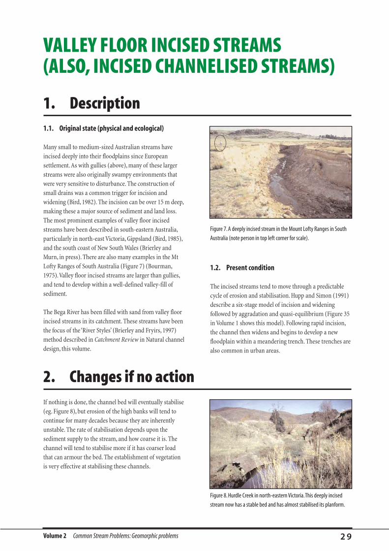
Figure 7. A deeply incised stream in the Mount Lofty Ranges in South
Australia (note person in top left corner for scale).
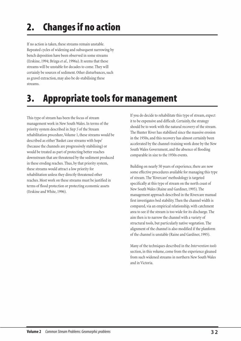
2. Changes if no actionIf nothing is done, the channel bed will eventually stabilise
(eg. Figure 8), but erosion of the high banks will tend to
continue for many decades because they are inherently
unstable. The rate of stabilisation depends upon the
sediment supply to the stream, and how coarse it is. The
channel will tend to stabilise more if it has coarser load
that can armour the bed. The establishment of vegetation
is very effective at stabilising these channels.
Figure 8. Hurdle Creek in north-eastern Victoria.This deeply incised
stream now has a stable bed and has almost stabilised its planform.
Volume 2 Common Stream Problems: Geomorphic problems 3 0
Although these erosion trenches look spectacular, they
afflict only a small proportion of Australian streams. For
true ecological rehabilitation of streams, the main
problems with these trenches are:
• as barriers to animal migration to higher reaches
(when they flow it is at high velocity, with limited base-
flow between such events); and
• as a source of fine sediment downstream (they can
contaminate long reaches of stream). This fine
sediment is hard to manage because it comes from
high, raw banks.
Large incised streams would receive higher priority if the
fine sediment that they produce was threatening high-
value reaches downstream.
If it is necessary to stabilise large incised streams, then the
same principles of management apply as for gullies, except
that valley floor incised streams are tremendously
powerful. The management principles are:
• aim to accelerate the natural process of recovery;
• always stabilise the bed before the bank (see Full width
structures, in Intervention in the channel, this volume);
• encourage invasion of the channel bed by vegetation to
accelerate stability; and
• wherever possible divert high flows out of the channel,
but encourage low flows to assist revegetation.
3. Ecological significance
In most cases, large incised streams fall into the ‘Basket
case with hope’ category of our prioritisation procedure
(see Step 5: Setting priorities, in the planning procedure,
Volume 1). Thus, if natural stream rehabilitation is your
primary concern, then this type of stream would receive
low priority. In fact, they would probably have the lowest
priority of any stream, because they have considerable
potential for recovering on their own (given sufficient
sediment and vegetation). This is an important point
because this type of stream has traditionally attracted
large amounts of money, often justified on vaguely
ecological grounds.
4. Appropriate tools for management

Volume 2 Common Stream Problems: Geomorphic problems 3 1
1.1. Original state (physical and ecological)
Some Australian streams have transformed from reputedly
stable, narrow, suspended-load dominated, sinuous
channels, into broad, unstable, bedload-dominated
channels (see Figure 9). Catastrophic channel enlargement
(largely through widening) is recorded on coastal streams
from Gippsland in the south to the Queensland tropics in
the north. The best-documented examples occur in the
coastal streams of New South Wales. Stream managers in
Queensland often argue that their streams are periodically
widened during cyclones, and narrow again between
them. Cattle Creek is an example of such change (Brizga
et al., 1996a). The enlargement can take place anywhere
along the channel, but is most common in confined
sections of floodplain, and close to the point where the
streams leave the mountain front (Warner, 1992).
More money has probably been spent on this spectacular
channel change than any other stream management issue
in Australia (with the possible exception of gullying). For
example, the New South Wales Department of Water
Resources spent $132 million (estimated minimum 1993
dollars) on 90 major and 436 minor river training and
channelisation schemes in the Hunter River catchment
alone following dramatic enlargement during a series of
floods between 1949 and 1955 (Erskine, 1990b; Erskine,
1992a).
1.2. Channel destruction
In response to a single unusually large flood, or series of
floods, some channels will dramatically enlarge. This
enlargement is usually a result of great increases in width,
which may be associated with increased meander
migration. Other changes include channel straightening
from chute cut-offs. The bed may degrade, but it may
aggrade as a pulse of sediment from the eroded reach
moves down the stream system. The expanded trench then
behaves like the valley floor incised streams (described in
Valley floor incised streams, above). In the decades
following the channel changes, the over-widened trench
often narrows as vegetation encroaches, the thalweg
deepens, benches form, and the channel regains its
sinuosity. Reaches downstream can be choked with sand
and gravel liberated from the erosion (Erskine, 1993;
Erskine, 1996).
There is considerable debate about why these streams
erode so dramatically (see, for example, Erskine and
Warner, 1998; Kirkup et al., 1998). Although the erosion is
triggered by major floods, it is likely that clearing of
riparian vegetation plays a role in weakening the banks,
leading to the major erosion (Brooks, 1999). The ecological
effects of the channel changes may be dramatic. Habitat in
the streams can be considerably simplified.
LARGER OVER-WIDENED STREAMS
1. Description
Figure 9.The Avon River, Gippsland. An example of a stream that has
widened dramatically over the last 150 years.
Volume 2 Common Stream Problems: Geomorphic problems 3 2
If no action is taken, these streams remain unstable.
Repeated cycles of widening and subsequent narrowing by
bench deposition have been observed in some streams
(Erskine, 1994; Brizga et al., 1996a). It seems that these
streams will be unstable for decades to come. They will
certainly be sources of sediment. Other disturbances, such
as gravel extraction, may also be de-stabilising these
streams.
This type of stream has been the focus of stream
management work in New South Wales. In terms of the
priority system described in Step 5 of the Stream
rehabilitation procedure,Volume 1, these streams would be
described as either ‘Basket case streams with hope’
(because the channels are progressively stabilising) or
would be treated as part of protecting better reaches
downstream that are threatened by the sediment produced
in these eroding reaches. Thus, by that priority system,
these streams would attract a low priority for
rehabilitation unless they directly threatened other
reaches. Most work on these streams must be justified in
terms of flood protection or protecting economic assets
(Erskine and White, 1996).
If you do decide to rehabilitate this type of stream, expect
it to be expensive and difficult. Certainly, the strategy
should be to work with the natural recovery of the stream.
The Hunter River has stabilised since the massive erosion
in the 1950s, and this recovery has almost certainly been
accelerated by the channel-training work done by the New
South Wales Government, and the absence of flooding
comparable in size to the 1950s events.
Building on nearly 50 years of experience, there are now
some effective procedures available for managing this type
of stream. The ‘Rivercare’ methodology is targeted
specifically at this type of stream on the north coast of
New South Wales (Raine and Gardiner, 1995). The
management approach described in the Rivercare manual
first investigates bed stability. Then the channel width is
compared, via an empirical relationship, with catchment
area to see if the stream is too wide for its discharge. The
aim then is to narrow the channel with a variety of
structural tools, but particularly native vegetation. The
alignment of the channel is also modified if the planform
of the channel is unstable (Raine and Gardiner, 1995).
Many of the techniques described in the Intervention tools
section, in this volume, come from the experience gleaned
from such widened streams in northern New South Wales
and in Victoria.
2. Changes if no action
3. Appropriate tools for management

Volume 2 Common Stream Problems: Geomorphic problems 3 3
The temptation is often to concentrate our efforts on the
most dramatically damaged streams (see the priorities
Step 5 in the Stream rehabilitation planning procedure). In
reality, we should perhaps be concentrating our efforts on
the many tens of thousand of kilometres of marginal,
slightly damaged rural streams across the continent.
We see this type of stream every day, and probably consider
it a low priority, stable stream (eg. Figure 10). These streams
are typically quite small, they flow only occasionally, they are
often cleared to the banks, and stock have access to them.
The channel is eroding at the outer banks, and possibly has
deepened by half-a-metre or so. This enlargement is usually
due to grazing, combined with the increase in the size of
flood peaks coming from the cleared catchment. Large snags
may even have been removed because they were causing
erosion and possibly some flooding.
Any coarse sediments in the bed are probably
contaminated with fine sediment. Not much lives in the
stream, apart from carp, and possibly a platypus in the few
deep pools remaining. There is little shade and pools tend
to be slightly nutrient enriched.
The creek is unlikely to change its condition much if it is left
alone.With continued grazing and a cleared catchment there
is little prospect for natural recovery in this type of stream.
TYPICAL SMALL, ENLARGED RURAL STREAMS
1. Introduction
Figure 10. A typical degraded rural stream flowing off the Illawarra
escarpment in coastal New South Wales. Note the slight enlargement,
poor riparian vegetation, and ‘lumpy’ slumped banks.
The degraded rural stream described above is probably
the most typical stream type in the settled areas of
Australia. These streams can have considerable capacity
for recovery. They are small enough that moderate
management measures can pay rich rehabilitation
dividends. For example, they can be effectively shaded by
modest riparian vegetation. Thus, this type of stream
could well be a priority for rehabilitation, especially if up
or downstream there are sources of plants and animals
available for natural colonisation.
2. Ecological significance
What are we to do with such streams? The first response is
usually to think of stock exclusion, fencing and riparian
vegetation. This is quite right. The main problem is how
much can be achieved when probably most of the catchment
is in this sort of condition. Certainly, the emphasis must be
on working down from any remaining pockets of stream in
good condition. It is worth looking at any reaches that are
fenced and do have riparian vegetation. Do they enjoy better
in-channel structure, more macro-invertebrates, deeper
pools? If so, then there is your template for action. If not, then
you will have to look for other limiting variables. If there is
no obvious source of animal or plant colonists, then you have
to be realistic about how long it will take revegetated reaches
to recover—probably decades.
3. Appropriate tools for management
Volume 2 Common Stream Problems: Geomorphic problems 3 4
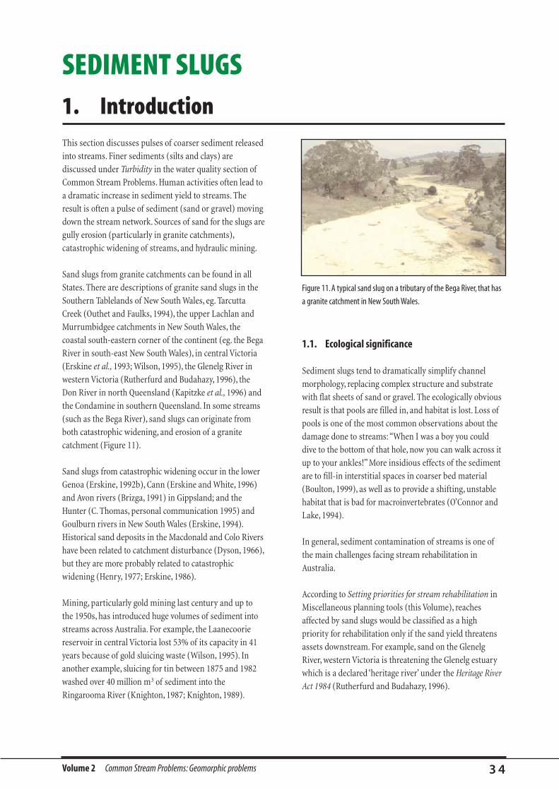
This section discusses pulses of coarser sediment released
into streams. Finer sediments (silts and clays) are
discussed under Turbidity in the water quality section of
Common Stream Problems. Human activities often lead to
a dramatic increase in sediment yield to streams. The
result is often a pulse of sediment (sand or gravel) moving
down the stream network. Sources of sand for the slugs are
gully erosion (particularly in granite catchments),
catastrophic widening of streams, and hydraulic mining.
Sand slugs from granite catchments can be found in all
States. There are descriptions of granite sand slugs in the
Southern Tablelands of New South Wales, eg. Tarcutta
Creek (Outhet and Faulks, 1994), the upper Lachlan and
Murrumbidgee catchments in New South Wales, the
coastal south-eastern corner of the continent (eg. the Bega
River in south-east New South Wales), in central Victoria
(Erskine et al., 1993; Wilson, 1995), the Glenelg River in
western Victoria (Rutherfurd and Budahazy, 1996), the
Don River in north Queensland (Kapitzke et al., 1996) and
the Condamine in southern Queensland. In some streams
(such as the Bega River), sand slugs can originate from
both catastrophic widening, and erosion of a granite
catchment (Figure 11).
Sand slugs from catastrophic widening occur in the lower
Genoa (Erskine, 1992b), Cann (Erskine and White, 1996)
and Avon rivers (Brizga, 1991) in Gippsland; and the
Hunter (C. Thomas, personal communication 1995) and
Goulburn rivers in New South Wales (Erskine, 1994).
Historical sand deposits in the Macdonald and Colo Rivers
have been related to catchment disturbance (Dyson, 1966),
but they are more probably related to catastrophic
widening (Henry, 1977; Erskine, 1986).
Mining, particularly gold mining last century and up to
the 1950s, has introduced huge volumes of sediment into
streams across Australia. For example, the Laanecoorie
reservoir in central Victoria lost 53% of its capacity in 41
years because of gold sluicing waste (Wilson, 1995). In
another example, sluicing for tin between 1875 and 1982
washed over 40 million m3 of sediment into the
Ringarooma River (Knighton, 1987; Knighton, 1989).
1.1. Ecological significance
Sediment slugs tend to dramatically simplify channel
morphology, replacing complex structure and substrate
with flat sheets of sand or gravel. The ecologically obvious
result is that pools are filled in, and habitat is lost. Loss of
pools is one of the most common observations about the
damage done to streams: “When I was a boy you could
dive to the bottom of that hole, now you can walk across it
up to your ankles!” More insidious effects of the sediment
are to fill-in interstitial spaces in coarser bed material
(Boulton, 1999), as well as to provide a shifting, unstable
habitat that is bad for macroinvertebrates (O’Connor and
Lake, 1994).
In general, sediment contamination of streams is one of
the main challenges facing stream rehabilitation in
Australia.
According to Setting priorities for stream rehabilitation in
Miscellaneous planning tools (this Volume), reaches
affected by sand slugs would be classified as a high
priority for rehabilitation only if the sand yield threatens
assets downstream. For example, sand on the Glenelg
River, western Victoria is threatening the Glenelg estuary
which is a declared ‘heritage river’ under the Heritage River
Act 1984 (Rutherfurd and Budahazy, 1996).
SEDIMENT SLUGS1. Introduction
Figure 11. A typical sand slug on a tributary of the Bega River, that has
a granite catchment in New South Wales.
Volume 2 Common Stream Problems: Geomorphic problems 3 5
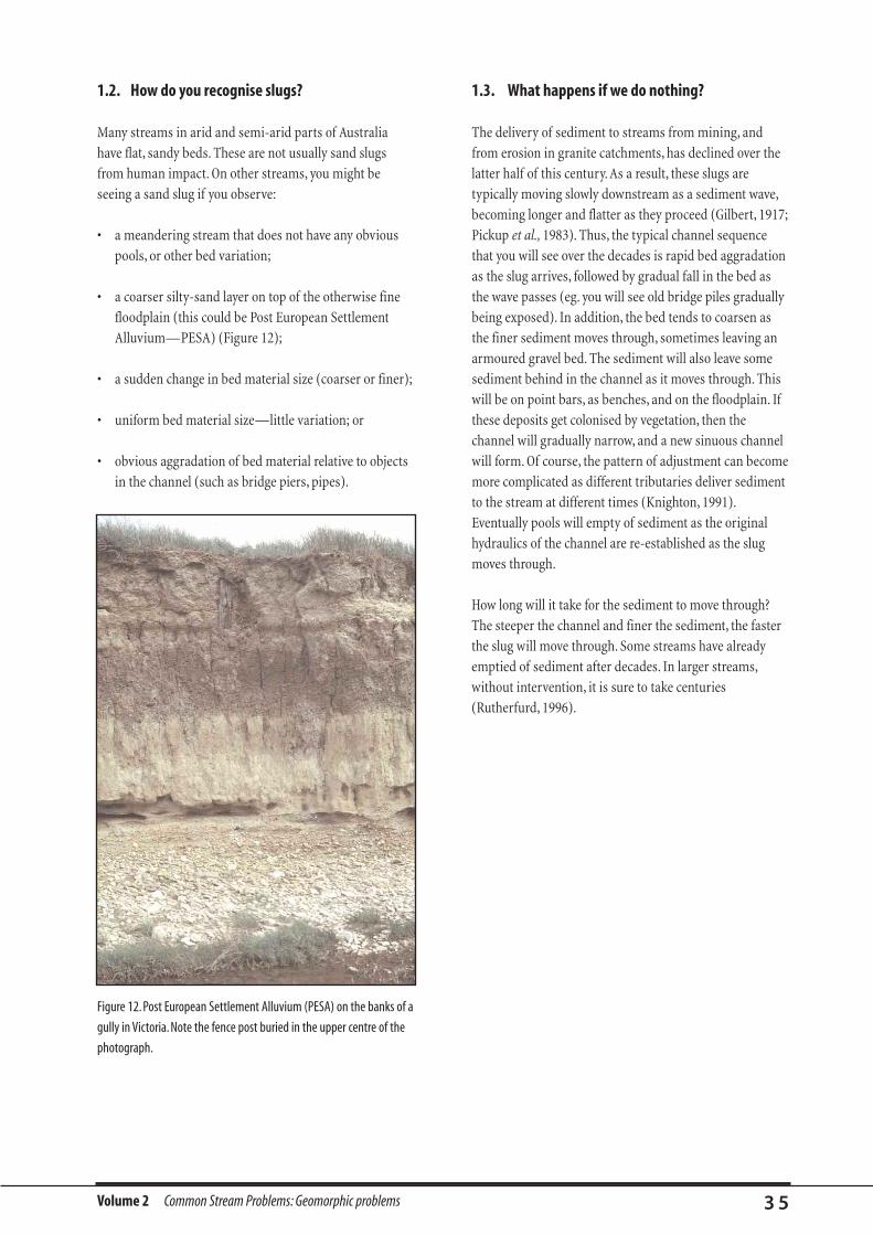
1.2. How do you recognise slugs?
Many streams in arid and semi-arid parts of Australia
have flat, sandy beds. These are not usually sand slugs
from human impact. On other streams, you might be
seeing a sand slug if you observe:
• a meandering stream that does not have any obvious
pools, or other bed variation;
• a coarser silty-sand layer on top of the otherwise fine
floodplain (this could be Post European Settlement
Alluvium—PESA) (Figure 12);
• a sudden change in bed material size (coarser or finer);
• uniform bed material size—little variation; or
• obvious aggradation of bed material relative to objects
in the channel (such as bridge piers, pipes).
1.3. What happens if we do nothing?
The delivery of sediment to streams from mining, and
from erosion in granite catchments, has declined over the
latter half of this century. As a result, these slugs are
typically moving slowly downstream as a sediment wave,
becoming longer and flatter as they proceed (Gilbert, 1917;
Pickup et al., 1983). Thus, the typical channel sequence
that you will see over the decades is rapid bed aggradation
as the slug arrives, followed by gradual fall in the bed as
the wave passes (eg. you will see old bridge piles gradually
being exposed). In addition, the bed tends to coarsen as
the finer sediment moves through, sometimes leaving an
armoured gravel bed. The sediment will also leave some
sediment behind in the channel as it moves through. This
will be on point bars, as benches, and on the floodplain. If
these deposits get colonised by vegetation, then the
channel will gradually narrow, and a new sinuous channel
will form. Of course, the pattern of adjustment can become
more complicated as different tributaries deliver sediment
to the stream at different times (Knighton, 1991).
Eventually pools will empty of sediment as the original
hydraulics of the channel are re-established as the slug
moves through.
How long will it take for the sediment to move through?
The steeper the channel and finer the sediment, the faster
the slug will move through. Some streams have already
emptied of sediment after decades. In larger streams,
without intervention, it is sure to take centuries
(Rutherfurd, 1996).
Figure 12. Post European Settlement Alluvium (PESA) on the banks of a
gully in Victoria. Note the fence post buried in the upper centre of the
photograph.

Volume 2 Common Stream Problems: Geomorphic problems 3 6
There are three main options for managing sand slugs:
1. Intercept sand from upstream. A weir or other
structure can catch sand as it moves downstream. This
will tend to clean the sediment out below the structure.
Reducing the input of sediment in the first place is the
most obvious option. This, however, could take decades
to translate into a fall in bed levels downstream.
2. Artificially remove the sand. Sand and gravel
extraction as a rehabilitation tool, in Intervention tools,
this Volume, discusses the use of sand and gravel
extraction as a management tool. There are many cases
where extraction is the only real management option.
With commercial extraction, this is sometimes viable,
but only if you are able to remove material at the rate
that it is transported into the reach, or greater.
3. Stabilise the sand and constrict the channel.
Sometimes it is possible to gradually stabilise the
sediment with vegetation. This will then constrict the
channel and may maintain a deeper channel.
Structures can also artificially constrict the channel
(eg. groynes and retards).
2. Appropriate tools for management

WATER QUALITYPROBLEMS
• Water quality: an introduction
• Fine sediments and turbidity
• Nutrient enrichment
• Dissolved oxygen concentration
• High and low temperatures
• Salinity
• Toxicants

Volume 2 Common Stream Problems: Water quality problems 3 8
There is a wide variety of water quality problems which
can affect our streams. However, only those that affect
stream ecology are of concern to us in this manual, thus
leaving out of consideration parameters important for
drinking water, such as faecal coliforms, taste and odour.
There are six ecologically important categories of water
quality problem:
1. turbidity and fine sediments, that will restrict the area
where photosynthesis can occur, clog the gills and guts
of animals, and smother the stream bed;
2. nutrients that, under certain environmental conditions,
will lead to nuisance plant growth, and in extreme
cases eutrophication;
3. low dissolved oxygen that will cause the suffocation of
stream organisms;
4. high and low temperature that will affect dissolved
oxygen levels and the metabolism of stream fauna;
5. salinity that can have toxic effects on stream
organisms, and also reduces dissolved oxygen
concentrations; and
6. toxicants, a large group of toxic materials that includes
heavy metals, oils, pesticides and herbicides, and a
large variety of naturally occurring and synthetic
chemicals used in fuels, manufacturing, and just about
anything else one can think of.
WATER QUALITY: AN INTRODUCTION
Every water quality problem shares some common
attributes.
1.1. The natural concentrations were variable andare now difficult to determine
Except for the synthetic toxicants, all of these forms of
water pollution did exist naturally, although usually not to
the extent now seen. Lowland rivers have probably always
had higher turbidity and nutrient levels and temperatures
than mountain streams. Terminal river systems, such as in
the Wimmera River in Victoria’s west, are naturally saline.
Such lowland streams, with warmer, more saline waters,
would always have had lower oxygen levels than cold,
turbulent mountain streams. Even heavy metals are found
naturally (in very small concentrations) in some streams,
because of their presence in the local rock. It is clear that
the natural levels of these water quality parameters varied
from place to place, depending on geology, soils, climate
and topography. Unfortunately, but not surprisingly, no one
took too much notice of the natural levels during
European settlement, unless the quality was noticeably
bad. For example, Sturt commented on the salinity of the
Darling River in 1829 because the water was too salty for
him or his stock to drink (ANZECC, 1992a).
Why do the natural levels of these water quality parameters
matter? The purpose of this manual is to help rehabilitate
streams; that is, to return them to their natural state. If a
stream was naturally saline, turbid, and had high nutrient
loads, then these are not problems in terms of rehabilitation.
Indeed, they represent a distinct habitat, often with a
correspondingly distinct flora and fauna that should be
preserved.Also, it is unlikely that we would have any success
in ‘improving’ such problems beyond their natural condition.
So, the guidelines for water quality should reflect the
geographical variation in natural conditions.
Unfortunately, in most cases the natural conditions are not
known, and much historical, chemical and biological
detective work is required to work out what they might have
been. This means that almost all water quality guidelines are
either not always appropriate, or given as a range of
concentrations that are far too generalised to be very useful.
1. Common attributes of water quality problems
Please note:
That by mid-2000 a new version of the “Australian Water
Quality Guidelines for Fresh and Marine Systems “ is to be
published by the Australia and New Zealand Environment and
Conservation Council.These comprehensive guidelines will
probably supersede the following sections.
Volume 2 Common Stream Problems: Water quality problems 3 9
There are two possible approaches to narrowing this range to
make it more specific to your stream.You should consider
the potential effect of geology, soils, climate and topography,
in combination with searching for historical records of water
quality.A complementary approach would be to consider any
historical records of plants or animals once found in the
stream. The tolerances of these species (where these are
known) will be indicative of the natural water quality (see
Biological site assessment in Natural channel design, this
Volume).
1.2. The concentrations of pollutants vary withflow
Stream flow is a major determinant of the concentration of
pollutants. High flows will dilute some, while others
become more concentrated.
Dilution occurs for pollutants that are delivered to the
stream at a steady rate. For example, salts often enter
saline streams directly from salty groundwater. The rate at
which this occurs is not affected by a single flood.
However, because of the larger volume of fresh water, the
saline groundwater is diluted, and the salt concentration in
the stream will drop. A similar situation would occur
where there is a constant discharge of industrial
wastewater.
By contrast, some pollutants, such as turbidity and
nutrients, will become more concentrated during high
flows. There are two reasons for this. Firstly, these
pollutants are delivered to the stream chiefly by run-off,
which increases during rain. Another example is the mix
of toxicants that are washed off urban roads, houses and
gardens in the first hour of a storm. Secondly, during high
flows there is sufficient stream power to erode and
transport sediment in the channel. This combination of
factors results in high concentrations of these pollutants,
often peaking before the flood itself peaks. A general rule-
of-thumb is that 90% of sediment is transported in only
10% of the flow.
The variation in concentration with flow has serious
implications for water quality monitoring. Large
proportions of some pollutants are carried in peak flood
events, which are difficult to monitor—they have
unpredictable timing, and require multiple measurements
through the flood hydrograph as there is not a predictable
relationship between concentration of pollutants and flow.
1.3. The effects of pollution are not always well known
There has been relatively little research on the effects of
pollutants on the Australian aquatic biota. Mostly, the
guidelines are derived from northern hemisphere data.
While this may result in suitable guidelines for Australian
conditions, this will not always be the case. Trout, for
example, are more tolerant of cold water and more
sensitive to high temperatures than many native fish
species. Temperature guidelines based on this fish would
be inappropriate.
Mostly, water quality guidelines are based on the level of
pollution that causes death in an organism. However, long-
term exposure to lower levels of a pollutant may cause
stress, resulting in lower rates of growth and development,
which may flow through to lower reproductive success. Over
generations, this can lead to the local extinction of a species.
If there is considerable variation in natural water quality,
and in many cases we are uncertain of the effects of the
water quality on stream plants and animals, how will you
know if water quality is a problem in your stream? In the
following chapters, we present ‘Thresholds of concern’
for our six water quality problems. These are the levels at
which the pollutants in question are likely to become a
serious worry.
1.4. Options for biological monitoring
One way of getting around the problems of water quality
monitoring is through biological indicators. This involves
examining the species of plants or animals present in the
stream. Possible water quality problems will be indicated
by the sensitivity of species that are absent, and the
tolerances of species that are present.
There are several advantages to biological monitoring. To
an extent, it will bypass the issue of establishing accurate
thresholds of concern, because you are measuring the
biological effect directly, rather than relying on laboratory
studies of a few species to tell you what important
concentrations are. It also allows you to assess the
cumulative effect of pollutants in different flows. Moreover,
biological monitoring allows you to look for a large variety
of possible pollutants in one test. For more information on
this, see Biological site assessment in Natural channel
design, this volume.

Volume 2 Common Stream Problems: Water quality problems 4 0
Large quantities of fine sediment in streams will affect the
stream biota in three ways. When travelling in the water
column, the suspended sediment has optical effects, in
that it creates muddiness or cloudiness that reflects or
absorbs light. This effect is known as turbidity. Fine
sediment also has physical effects. During high flows,
sediment can abrade and scour plants and animals. At
lower flows, material may be deposited, and can reduce
habitat in the stream bed by filling the gaps between larger
bed material, smothering benthic invertebrates, algae and
fish eggs in the process.
1.1. Natural state
There is little doubt that, before European disturbance of
catchments and channels, levels of turbidity and unstable
fine sediment in many of Australia’s streams would have
been much lower than present levels, particularly at base
flow. Flood events would naturally have been turbid,
though again possibly not to the extent of present day
floods. Australian rivers are generally thought to have high
natural turbidity, because of the naturally sparse
vegetation cover and high levels of fine clay in the readily
erodible soils (Kirk, 1985). It is assumed that aquatic
plants and animals have adapted to these levels. However,
the lack of historical data means it is unclear just how
turbid rivers would naturally be. Anecdotal evidence
suggests that the Brisbane River (Stock and Neller, 1990),
and even inland rivers such as the Lachlan and the
Murray, were ‘clear’ until the early part of this century.
For undisturbed rivers at base flows, suspended sediment
and turbidity levels are usually quite low, around 5 NTU
(Nephelometric Turbidity Units) or 2–5 mg/L (Parliament of
Victoria, 1994). During floods, fast-flowing streams are able
to carry a lot more sediment, which may be eroded from the
stream bed and banks, and also by the floodplain run-off.
However, in undisturbed streams the increases in turbidity
during floods are relatively small; in the order of 100 NTU in
the southern States (Parliament of Victoria, 1994).
1.2. How has it changed
A variety of land management practices has contributed to
increased levels of turbidity and sedimentation. In-
channel sources of fine material include channel erosion,
instream works such as bridge and dam construction, and
sand and gravel extraction. Out of channel sources include
run-off from tilled land and farm tracks, forestry tracks
and stream crossings in upland areas, and run-off from
urban areas and construction areas.
Extreme examples of the gross effects of accumulated
sediment can be found in some lowland streams in the
cane lands of far north Queensland. Bunn et al. (1997)
estimated that approximately 20,000 tonnes of inorganic
sediment had accumulated per kilometre of stream
channel in the exotic ‘Para’ grass in Bamboo Creek, near
Innisfail. Oxygen penetration was limited to a few
millimetres and few benthic invertebrates were recorded
by Bunn et al. (1997) in their study of the food web.
TURBIDITY AND FINE SEDIMENT1. Introduction
2.1. Aquatic plants
Aquatic plants include macrophytes and benthic and
planktonic algae. Benthic algae refers to the mixture of
algae, diatoms, bacteria and fungi which forms the
‘biofilm’ on submerged surfaces. This layer is the food
source for many macroinvertebrates.
Fine sediment: Benthic algae is susceptible to damage in
turbid environments by the scouring and abrading effect of
the mobile sediment during high flows. Deposition of the
suspended sediment is also a problem as it will smother
algal growth. Even when very little deposition occurs,
sediment can adhere to the biofilm and reduce its potential
as a food source. Emergent aquatic plants such as water
ribbons (Triglochin spp.) and cumbungi (Typha spp.) are
less vulnerable to damage by high sediment loads, because
their photosynthetically active areas are above the water.
2. Biological impacts of turbidity and fine sediment
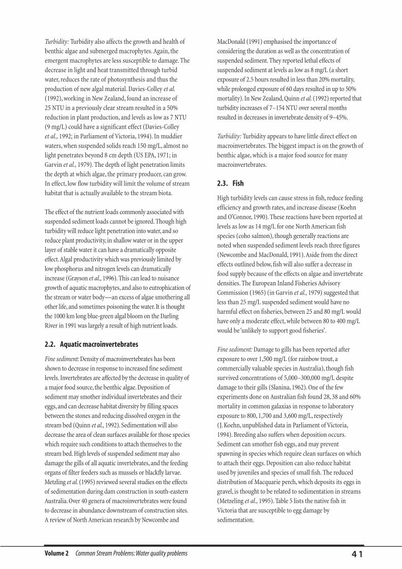
Volume 2 Common Stream Problems: Water quality problems 4 1
Turbidity: Turbidity also affects the growth and health of
benthic algae and submerged macrophytes. Again, the
emergent macrophytes are less susceptible to damage. The
decrease in light and heat transmitted through turbid
water, reduces the rate of photosynthesis and thus the
production of new algal material. Davies-Colley et al.
(1992), working in New Zealand, found an increase of
25 NTU in a previously clear stream resulted in a 50%
reduction in plant production, and levels as low as 7 NTU
(9 mg/L) could have a significant effect (Davies-Colley
et al., 1992; in Parliament of Victoria, 1994). In muddier
waters, when suspended solids reach 150 mg/L, almost no
light penetrates beyond 8 cm depth (US EPA, 1971; in
Garvin et al., 1979). The depth of light penetration limits
the depth at which algae, the primary producer, can grow.
In effect, low flow turbidity will limit the volume of stream
habitat that is actually available to the stream biota.
The effect of the nutrient loads commonly associated with
suspended sediment loads cannot be ignored. Though high
turbidity will reduce light penetration into water, and so
reduce plant productivity, in shallow water or in the upper
layer of stable water it can have a dramatically opposite
effect.Algal productivity which was previously limited by
low phosphorus and nitrogen levels can dramatically
increase (Grayson et al., 1996). This can lead to nuisance
growth of aquatic macrophytes, and also to eutrophication of
the stream or water body—an excess of algae smothering all
other life, and sometimes poisoning the water. It is thought
the 1000 km long blue-green algal bloom on the Darling
River in 1991 was largely a result of high nutrient loads.
2.2. Aquatic macroinvertebrates
Fine sediment: Density of macroinvertebrates has been
shown to decrease in response to increased fine sediment
levels. Invertebrates are affected by the decrease in quality of
a major food source, the benthic algae. Deposition of
sediment may smother individual invertebrates and their
eggs, and can decrease habitat diversity by filling spaces
between the stones and reducing dissolved oxygen in the
stream bed (Quinn et al., 1992). Sedimentation will also
decrease the area of clean surfaces available for those species
which require such conditions to attach themselves to the
stream bed. High levels of suspended sediment may also
damage the gills of all aquatic invertebrates, and the feeding
organs of filter feeders such as mussels or blackfly larvae.
Metzling et al. (1995) reviewed several studies on the effects
of sedimentation during dam construction in south-eastern
Australia. Over 40 genera of macroinvertebrates were found
to decrease in abundance downstream of construction sites.
A review of North American research by Newcombe and
MacDonald (1991) emphasised the importance of
considering the duration as well as the concentration of
suspended sediment. They reported lethal effects of
suspended sediment at levels as low as 8 mg/L (a short
exposure of 2.5 hours resulted in less than 20% mortality,
while prolonged exposure of 60 days resulted in up to 50%
mortality). In New Zealand, Quinn et al. (1992) reported that
turbidity increases of 7–154 NTU over several months
resulted in decreases in invertebrate density of 9–45%.
Turbidity: Turbidity appears to have little direct effect on
macroinvertebrates. The biggest impact is on the growth of
benthic algae, which is a major food source for many
macroinvertebrates.
2.3. Fish
High turbidity levels can cause stress in fish, reduce feeding
efficiency and growth rates, and increase disease (Koehn
and O’Connor, 1990). These reactions have been reported at
levels as low as 14 mg/L for one North American fish
species (coho salmon), though generally reactions are
noted when suspended sediment levels reach three figures
(Newcombe and MacDonald, 1991).Aside from the direct
effects outlined below, fish will also suffer a decrease in
food supply because of the effects on algae and invertebrate
densities. The European Inland Fisheries Advisory
Commission (1965) (in Garvin et al., 1979) suggested that
less than 25 mg/L suspended sediment would have no
harmful effect on fisheries, between 25 and 80 mg/L would
have only a moderate effect, while between 80 to 400 mg/L
would be ‘unlikely to support good fisheries’.
Fine sediment: Damage to gills has been reported after
exposure to over 1,500 mg/L (for rainbow trout, a
commercially valuable species in Australia), though fish
survived concentrations of 5,000–300,000 mg/L despite
damage to their gills (Slanina, 1962). One of the few
experiments done on Australian fish found 28, 38 and 60%
mortality in common galaxias in response to laboratory
exposure to 800, 1,700 and 3,600 mg/L, respectively
(J. Koehn, unpublished data in Parliament of Victoria,
1994). Breeding also suffers when deposition occurs.
Sediment can smother fish eggs, and may prevent
spawning in species which require clean surfaces on which
to attach their eggs. Deposition can also reduce habitat
used by juveniles and species of small fish. The reduced
distribution of Macquarie perch, which deposits its eggs in
gravel, is thought to be related to sedimentation in streams
(Metzeling et al., 1995). Table 5 lists the native fish in
Victoria that are susceptible to egg damage by
sedimentation.

Volume 2 Common Stream Problems: Water quality problems 4 2
Turbidity: The effects of turbidity on fish are not known,
but it is likely that significant turbidity would reduce the
hunting success of those carnivorous species which rely on
sight to catch their food.
2.4. Frogs
Frog eggs, like fish eggs, are prone to smothering by
deposition of sediment. Once hatched, tadpoles rely on
gills to extract oxygen from the water. Like fish and
macroinvertebrates, they are susceptible to damage under
extremely turbid conditions, as are the feeding organs of
those species which filter feed. Other species graze on
algae, and will thus suffer a reduction in food source as
lower light levels decrease algae productivity. Adult frogs
are less likely to be disadvantaged by high turbidity, as
they are largely terrestrial.
2.5. Reptiles
High levels of turbidity are unlikely to have a direct
adverse effect on reptiles (Parliament of Victoria, 1994).
However, species such as the long-necked tortoise and the
red-bellied black snake which rely on aquatic systems as a
food source may be affected by the decreases in frog and
fish numbers.
2.6. Birds
Turbidity will affect the hunting success of kingfishers,
which need to see their prey. Small rises in turbidity are
sufficient to shield fish from the gaze of searching
kingfishers. The azure kingfisher, which relies solely on
aquatic food sources would be particularly disadvantaged.
2.6. Platypus
Platypus hunt with their eyes, ears and nostrils shut,
relying on the sensitive skin and electroreceptors in the bill
to detect the macroinvertebrates which are their prey
(Grant, 1995). As such, their hunting ability should not be
directly affected by high turbidity levels. However, they
may be affected by the decreases in macroinvertebrate
density.
2.7. Water rats
Water rats do not depend solely on aquatic systems for
food, though much of their food does come from this
environment. As such, it is likely they are able to find
alternative food sources, at least during short term
turbidity events.
Species Conservation status
Geotria australis (pouched lamprey) Potentially threatened
Galaxias oldidus (mountain galaxias) Indeterminate
Galaxias brevipinnis (climbing galaxias) Potentially threatened
Galaxias rostratus (flat-headed galaxias) Indeterminate
Retropinna semoni (Australian smelt) Common/widespread
Protrocetes maraena (Australian grayling) Vulnerable
Tandanus tandanus (freshwater catfish) Vulnerable
Craterocephalus stercusmuscarum (freshwater hardyhead) Indeterminate
Nannoperca australis (southern pygmy perch) Common/widespread
Gobiomorphus coxii (Cox’s gudgeon) Indeterminate
Maccullochella peelii (Murray cod) Vulnerable
Maccullochella macquariensis (trout cod) Endangered
Arenigobius bifrenatus (bridled goby) Common/widespread
Table 5. Native Victorian fish species which lay eggs on or amongst the stream bed and would be liable to smothering due to increased sediment
deposition. Source Metzeling et al. (1995), adapted from Koehn and Morison (1990).

Volume 2 Common Stream Problems: Water quality problems 4 3
When considering the reasons for a lack of stream biota
(or perhaps an excess of algae), it is important to
remember turbidity is only one of many aspects of water
quality that could be responsible. High turbidity is often
correlated with the presence of other pollutants, such as
fertilisers, pesticides and heavy metals. This is partly
because these are often transported bound to sediment
particles. However, there may be more efficient ways of
tackling water quality problems than through turbidity
alone. In some cases, turbidity may not be high enough to
cause problems in itself, but the chemicals associated with
that turbidity can have major impacts on the stream. The
main sources of sediment may not be the main sources of
nutrients and toxic compounds. All aspects of water
quality should be considered when attempting to reinstate
the stream biota.
3. Other water quality issues
4.1. Field characteristics
Fine sediment: Suspended sediment refers to the load of
sediment carried in suspension in the water rather than
moving on the bed of the stream. Without actually
measuring this sediment, it is not easy to judge how much
is present. The turbidity of water is an unreliable guide to
the amount of suspended sediment present, as different
sized particles have different optical effects. Fine sand in
suspension will have a less muddy appearance than a
much smaller quantity of clay.
After high flows, the coarser portion of suspended
sediment will settle on the stream bed, where it will
smother invertebrates and algae. From here it can be
resuspended in subsequent high flows. It can be difficult to
tell if such deposition is occurring on a stream bed, as
some fine material is naturally present in most systems.
However, if silt or mud is blanketing the stream bed or
totally filling spaces beneath gravel and cobbles, it is likely
there is a problem.
Turbidity: While suspended, the turbidity effect of fine
sediment is easily recognisable as cloudy or muddy water.
At low levels, variation in turbidity can be detected by eye,
but it is important to be aware that the depth you look
through will influence how turbid the water seems to be.
Purely visual surveys of turbidity are not accurate.
4.2. Measurement techniques
Fine sediment: Ignoring the more complex issues of
suspended sediment distribution through the stream,
measurement is a simple matter of taking a water sample
of known volume, and filtering, drying and weighing the
sediment. The results are expressed as milligrams of
sediment per litre of water (mg/L).
Turbidity: Turbidity is a measure of how the suspended
sediment affects visibility. Turbidity is measured by the
amount of light reflected or absorbed as it passes through
the water (usually in NTU—Nephelometric Turbidity
Units).
Table 6 gives some idea of how turbidity and suspended
sediment levels relate to the water you see around you.
4. How do you recognise turbidity and fine sediment?

Volume 2 Common Stream Problems: Water quality problems 4 4
A big issue with measurement of turbidity and suspended
sediment is the great variability in concentrations observed
at different flows. By far the highest turbidity, and greatest
quantity of suspended sediment is transported during
peak flows (about 90% of the sediment is transported in
less than 10% of the time in most streams). This poses
several problems. Firstly, do you attempt to take
measurements during high flows, and secondly, which
flows will actually cause problems for the stream biota? The
impact of fine sediment and turbidity on stream biota
depends on the duration as well as the intensity.As far as
turbidity is concerned, it may well be the extended low flow
levels that are critical; thus, this is probably what should be
measured. Conversely, the scouring effects of fine
sediments occur at high flows, and the smothering effects
are probably greatest just after periods of high flow.
Where turbidity is caused by organic rather than inorganic
solids, such as downstream of a sewage farm or a wood-
pulping plant, decomposition of the organics can
dramatically lower the dissolved oxygen and suffocate the
stream biota. Inorganic turbidity composed of metal
particulates can have toxic effects beyond those of
biologically inactive sediment. The following comments
relate to inactive inorganic sediment, though they may also
be applicable to organic and toxic sediment.
NTU mg/L
5 NK Maximum turbidity for drinking water (just visible in a glass of water) (NHMRC Environmental Health Committee, 1994).
5 2–5 Natural levels for Victorian highland streams at base flow (Parliament of Victoria, 1994).
5.3 10 Yarra River at Launching Place,Victoria (well before it reaches Melbourne) (unpublished EPA data in Parliament of Victoria (1994)).
32 50 Yarra River at the Chandler Highway, in Melbourne,Victoria (unpublished EPA data in Parliament of Victoria (1994)).
1 NK Mitchell River, Queensland, normal background levels (Frankcombe and Whitfield (1992); in Parliament of Victoria (1994)).
70–80 NK Mitchell River, Queensland, in times of flood (Frankcombe and Whitfield (1992); in Parliament of Victoria (1994)).
NK 705 Mean during a flood (recurrence 1 in 2) on the Annan River, northern Queensland (Hart and McKelvie, 1986).
NK 12 Mean during low flows on the Annan River, northern Queensland (Hart and McKelvie, 1986).
NK 40 Murray River at low flow (Ian Rutherfurd, personal communication).
NK 300 Murray River at high flow (Ian Rutherfurd, personal communication).
NK 3000 The Queen River,Tasmania (Locher, 1996).
The impact of a turbidity event depends on its intensity and
the duration (Newcombe and MacDonald, 1991).Thus, long-
term low levels of suspended sediment can have effects on the
stream biota as profound as much higher levels lasting only a
short time.
As mentioned above, the great difficulty in measuring
turbidity and suspended sediment is the huge variation in
concentrations depending on flow.The same can be said for
setting reasonable guidelines for turbidity.Even in the best
systems, an extreme flood could be accompanied by extreme
turbidity.The best way to get around this problem is to look at
the frequency distribution of turbidity levels.For example,
the Victorian EPA (EPA State Environment Policy in
Parliament of Victoria, 1994) requires suspended sediment to
be below 80 mg/L for 90% of the time.The Index of Stream
Condition (DNRE, 1997a) uses a similar system, examining
turbidity in terms of the median value (that is, at this point,
50% of the readings fall above the median, and 50% fall
below).This system does require regular monitoring in order
to get an appreciation of the range of values.Table 7 rates
various turbidity levels for Victorian streams.
5. At what stage does turbidity and fine sediment become a problem?
Table 6.Examples of levels of turbidity or suspended sediment concentration (mg/L) seen in water in Australian streams (NTU =Nephelometric Turbidity Units;
NK = data not known).

Volume 2 Common Stream Problems: Water quality problems 4 5
It is beyond the scope of this manual to provide
information on controlling erosion and suspended
sediment. There are detailed guides that assist with the
three approaches to managing turbidity: (a) reducing the
erosion at its source; (b) trapping the sediment before it
reaches the stream; and (c) trapping the sediment in the
stream. The most effective of these techniques is the first:
reducing the erosion rate. The finer sediment is, the less
effective sediment traps become, so dams, detention
basins and buffer strips are a second-best option for
managing sediment.
Reducing the erosion of sediment relies on identifying
where this erosion is occurring. There are many studies
that identify sediment sources and sinks (eg. Erskine and
Saynor, 1995), but most stream managers cannot afford to
do complex isotope tracing or sediment budget studies, or
measure large numbers of suspended sediment
concentrations. We would suggest that a good start for
stream managers (especially in small catchments) is to
hunt for turbidity sources themselves.
Turbidity cannot be accurately estimated by eye, because it
appears to increase with depth, when in fact the
suspended sediment concentration does not change.
Therefore, when hunting for turbidity sources, it is
important to use a turbidity meter. Take measurements of
turbidity throughout your stream network, perhaps
running down the trunk stream first. Divide the stream
into segments, based on tributary inputs and obvious
land-use boundaries. Sediment sources may vary,
depending on flow, so complete this survey at both high
and low flows. During low flows, the survey can be
completed over several days. However, during high flows,
the turbidity levels will change with the flow. For this
reason, a high flow turbidity survey should follow the flood
peak downstream. In such surveys, it is not unusual to find
that a single road crossing is the major source of turbidity
in a small catchment, as shown in Figure 13.
If you have identified a discrete sediment source such as a
gully, an eroding stream bank, a road culvert, or even a
particular type of land use in the catchment, then there is
a range of techniques available for you to manage the
erosion, such as revegetation, check banks, buffer strips,
and so on. A huge amount of information is available on
managing such point sources of erosion. We stress here
that the main problem is often identifying a source that
can be managed, not managing the sediment.
The most difficult problem is managing sediment from
diffuse general sources. Riparian vegetation may be a very
Mountain Valley Floodplain Rating
<5 <10 <15 Ideal
<7.5 <12.5 <17.5 Close to ideal
<10 <15 <20 Moderately different from ideal
<12.5 <22.5 <30 Substantially different from ideal
>12.5 >22.5 >30 Far from ideal
6. Possible treatments of turbidity
Figure 13. A plume of sediment entering a stream from a road crossing
in the headwaters of the Mary River, Queensland.
Table 7. Guidelines for median turbidity levels (NTU). From the Office of the Chief Commissioner for the Environment cited in DNRE, (1997a). Note that these
values are applicable only to streams in the south-east of Australia.
Volume 2 Common Stream Problems: Water quality problems 4 6
useful buffer, but this relies on run-off being filtered
through grass, leaf litter and soil. Often water will flow
through a buffer strip in small channels, and this will
dramatically reduce the effectiveness of the buffer strip.
Thus, wholesale riparian revegetation is not necessarily a
panacea for high turbidity levels. The Riparian Zone
Guidelines, published by LWRRDC, provide information
on buffer strips (see www.rivers.gov.au).
Key points aboutturbidity• Turbidity and fine sediment can damage organisms.
• Australian streams have very variable turbidity levels. Some
streams have naturally high turbidity.
• When monitoring, you need to distinguish between high
and low-flow turbidity.
• Is your problem high or low-flow turbidity? Each could
have a different source.
• A turbidity survey of your catchment could help to track
down whether there are obvious sources of high or low-
flow turbidity.
• Whilst there are many good techniques for managing
point sources of turbidity, managing diffuse sources
requires a catchment-wide and long-term approach.
• Turbidity can be difficult to manage, particularly if it is
associated with a high percentage of clay (ie. sediments
smaller than say 0.004 mm diameter).

Volume 2 Common Stream Problems: Water quality problems 4 7
High levels of the main plant nutrients, nitrogen and
phosphorus, can have important impacts on the biota of
our streams. Increasing the nutrients available can result
in increases in algae and macrophytes in the stream, in
extreme cases leading to blooms of toxic planktonic algae,
streams choked with macrophytes, or smothering of the
stream bed with algae. Extreme quantities of plant
material can severely deplete the oxygen in the water,
leading to fish kills. Even where plant growth is not
obviously excessive, nutrient levels may be high enough to
cause changes to invertebrate communities, and may have
the potential to cause algal blooms or eutrophication,
given the appropriate flow and temperature regime.
1.1. Natural state
Australia has some of the most nutrient-poor soils in the
world. It follows from this that natural nutrient levels
should also be low. Nevertheless, natural nutrient
concentrations are not the same across Australia: they vary
depending on variables such as geology, soil type, climate
and topography. An alpine stream will have naturally lower
nutrient levels than the lower Darling, for example. Present
nutrient levels in forest streams of south-western Western
Australia are so low they approach the extremely low
concentrations found in the open oceans. It is of course
impossible to establish with certainty the pre-European
levels of nutrients in those streams where land-use
changes and wastewater discharge have so altered water
quality (ie. most of Australia’s rivers). However, some
information is available from streams in relatively
untouched catchments, and from the relationship between
nutrient concentrations and the distribution of nutrient
sensitive invertebrate species. It is possible to make a good
judgment of at least the nutrient load that will not
adversely affect the healthy functioning of aquatic
ecosystems, if not the natural level. To the best of our
knowledge, such information exists only for Victoria,
in a report published by the Victorian EPA
(Tiller and Newall, 1995).
1.2. How it has changed
Diffuse and point source impacts such as nutrient-rich
run-off and irrigation wastewater from fertilised
farmland, erosion of nutrient-carrying sediment, animal
wastes, discharges from sewage-treatment plants, urban
drains and industrial sources of organic rich wastewater
have all contributed to increased nutrient loads in
Australia’s streams, in extreme cases two orders of
magnitude higher than estimated natural loads (ANZECC,
1992a). This increase is partly due to increases in
turbidity. Phosphorus readily becomes adsorbed onto clay
particles. This means that erosion of soil and stream banks
can be a significant source of nutrient. Once in the stream,
most of the phosphorus is transported with the clay. Thus,
high turbidity usually correlates with high levels of
phosphorus (Grayson et al., 1996).
NUTRIENT ENRICHMENT 1. Introduction
There are four ways in which nutrient enrichment can affect
stream ecology.You should remember that these effects will
be magnified at downstream sites where sediment and
nutrients collect in lakes, reservoirs and estuaries.
1. Relatively small increases in nutrient enrichment can
increase plant and algal productivity, which in turn
provides increased food for some invertebrate species.
This can result in sensitive species (eg. many stoneflies,
mayflies and caddis flies) being lost, and pollution-
tolerant species (eg. various snails, worms, and
chironomids) becoming more common.
2. In combination with appropriate environmental
conditions (light, temperature, flow etc.) nutrient
enrichment can lead to prolific growth of filamentous
green algae and macrophytes. These can reduce water
velocities and trap sediments and in extreme cases
effectively choke the stream channel resulting in a
considerable direct loss of aquatic habitat (see Bunn
et al., 1998). Such stands can form barriers to fish
passage.
2. Biological impacts of nutrient enrichment

Volume 2 Common Stream Problems: Water quality problems 4 8
3. Where conditions favour the development of
planktonic algae there is the possibility of an algal
bloom developing. The most famous example of this is
probably the algal bloom that turned over 1,000 km of
the Darling River bright green during November 1991.
In such situations, algae cell numbers can reach
surprisingly high levels (over 10 million cells per mL
(ANZECC, 1992a). Algal blooms cause the same
eutrophication problems as filamentous algae and
macrophytes. To make matters worse, cyanobacteria, or
blue-green algae, are often found in large numbers
during algal blooms. Also, some species of
cyanobacteria produce toxins, including liver toxins,
neurotoxins (attack nerves), cytotoxins (attack cells)
and endotoxins (mainly contact irritants).
4. When high nutrient levels and suitable environmental
conditions allow excessive plant growth, either of
macrophytes or algae, this can lead to eutrophication.
The decomposition of large quantities of plant
material, combined with the respiration needs of the
living plants, will deplete the water of oxygen, and alter
the pH, particularly in the deeper pools. This results in
the death of fish and macrocrustaceans. The same
process will occur if large quantities of organic waste
(eg. sewage, animal wastes) are dumped into streams.
Figure 14. Filamentous algae in a rural stream, probably associated
with high nutrients and water temperatures.
3.1. Field characteristics
The obvious way to recognise high-nutrient problems is
through searching for excess growth of algae and
macrophytes. Shallow, faster-flowing streams are prone to
infestations of filamentous algae and macrophytes, while
deeper, slower flowing rivers are more likely to suffer
planktonic (free floating) algal blooms (ANZECC, 1992a).
This is largely because light is often limiting in the larger
streams, and many planktonic algae can cope with this
problem by altering buoyancy to keep near the surface of the
water.
3.2. How to recognise algal blooms
While well-developed blooms are unmistakable, early stages,
or small blooms can be more difficult to detect.
• A bloom will increase the turbidity, because the algae
cells disperse through the water.
• The colour of the water will change.As the concentration of
cells increases,so does the amount of chlorophyll, the
green pigment in plants.Some blue-green algae form
floating colonies of hundreds of cells,which look like green
sawdust (Sainty and Jacobs,1994).
• As the bloom develops, a scum of cells may appear on the
water surface.
• Well-developed blooms may smell. Some species of blue-
green algae are ‘earthy or muddy smelling’ (Sainty and
Jacobs, 1994).Also, whatever the dominant species of
algae, when blooms are decaying, they can produce a
rancid, putrid smell.
There are two very important limits to using excess plant
growth to mark high nutrient levels.
1. An absence of nuisance plant growth does not
necessarily mean there is no nutrient problem.
Though prolific growths of macrophytes and algae do
indicate high nutrient levels, the absence of them does
not necessarily mean there is no problem. This is because
there are other factors which also regulate plant growth;
namely light, temperature, current velocity, substrate
3. How do you recognise nutrient enrichment ?
Volume 2 Common Stream Problems: Water quality problems 4 9
suitability and grazing pressure (ANZECC, 1992a).
Macrophytes require some fine sediment to root in, and,
as with filamentous and other attached algae, need a
stable bed. Plants and algae also need light, so deep
turbid streams are unlikely to develop infestations. This is
despite the way high turbidity often correlates with high
nutrient levels. Some planktonic algae can cope with
turbid water by altering buoyancy, and floating near the
surface. However, the turbulence of flowing water will
prevent these algae from remaining near the surface, and
so limit growth. For example, nutrient levels in the lower
Goulburn River in Victoria are probably always high
enough to sustain an algal bloom, but usually the low
light penetration through the turbid water, and the
turbulence in the moving water prevent a bloom from
developing (Tiller and Newall, 1995). Such nutrient-rich
streams will suffer blooms during periods of low flow
when turbidity and turbulence decrease.
2. Even if nutrient levels are not producing algal blooms at
your site, they may be causing a problem downstream.
Nutrients are transported downstream and will
accumulate in the sediments of lakes, reservoirs and
estuaries. Moderately high nutrients upstream may
eventually cause severe nutrient problems at these
downstream sites, so reducing nutrient inputs into
streams is always important.
3.3. Measurement techniques
Water samples should be taken from midstream, and about
mid-depth. Field test kits that measure nutrient
concentration are available, but tests done in an accredited
laboratory are more reliable. Talk to the laboratory about
what techniques you should use to preserve samples.
• How should you analyse the nutrient concentration in
your water sample? Water samples can be analysed using
field test kits, such as those used by Waterwatch, or sent
to a laboratory for analysis. Though the first option is
cheaper, there are two important limits to field test kits.
Firstly, they may be unable to detect low concentrations
of nutrients.As natural levels of nutrient are very low,
these tests will be unable to detect the smaller increases
in concentration. Secondly, such tests measure only the
dissolved nutrients, which will underestimate the
nutrient present. Nitrogen and phosphorus will attach to
fine sediment particles, and a significant proportion of
the nutrient will travel in this way rather than dissolved
in the water.Also, nutrient guidelines given here are
based on the total nutrient concentration, rather than the
dissolved fraction.
• Is there a existing monitoring program you can use?
There are already many groups who monitor water
quality, and it may be that enough information already
exists to assess the nutrient status of your stream.Ask the
EPA or equivalent in your State, as well as any local
bodies such as catchment management authorities.
When searching for relevant data, a single sampling site
can be indicative of the nutrient concentrations for 40 or
50 km upstream, so long as it is distant from point
sources of nutrients (and land use does not substantially
change) (David Tiller, EPA, Melbourne, personal
communication).
• Where should you sample? It is important to think
carefully about where you take samples. The sites you
choose will depend on whether you wish to assess the
impact of a possible point source of nutrients, or measure
the background level of nutrient. If you wish to monitor a
point source, then obviously you should sample just
downstream of that point source. However, if it is the
background nutrient levels then it is important to avoid
possible point sources.
• How often should you monitor? So long as the sample
was taken at a representative base flow (that is, not
during a drought, but not just after rain), one sample may
be indicative of the background nutrient concentrations
for that location. However, it is always safer to have more
than one sampling site if you want to be sure that your
measurements are representative of the water body.
• When should you measure? Nutrient concentrations vary,
depending partly on stream flow.The large majority of the
nutrient carried by a stream is moved during flood events,
when run-off delivers nutrient from the catchment
straight into the stream, and the high flows carry more
suspended sediment with its associated nutrient load. It is
the total annual nutrient load, dominated by peak flows,
that is most important to the ecology of lakes and
estuaries downstream.However, intensive sampling
during flood events is required to calculate this. It is the
concentration of nutrient in the water during base flow
that contributes to the growth of nuisance plants in
streams, so it is this measure that is used in Victoria’s
nutrient guidelines (Tiller and Newall, 1995).

Volume 2 Common Stream Problems: Water quality problems 5 0
present water quality. An updated set of guidelines is due
to be released towards the end of 1999.
4.3. Highlands river region
This region includes most areas in Victoria above 1000 m
altitude. Most of the area is minimally disturbed, and is
covered by forest or alpine vegetation. Streams are
typically small (less than 4 m), shallow and very clear.
Threshold of concern for total phosphorus 0.020 mg/L
Threshold of concern for total nitrogen 0.150 mg/L
4.4. Murray foothills river region
This region is part of the eastern Victorian uplands to the
north of the Great Dividing Range. Pre-European
vegetation ranged from open forest to woodland, but has
mostly been cleared and converted to pasture. Streams
typically have pool and riffle sequences and well-shaded
banks (where the riparian vegetation remains).
Threshold of concern for total phosphorus 0.030 mg/L
Threshold of concern for total nitrogen 0.200 mg/L
4.5. Southern and isolated foothills river region
This region is the southern equivalent of the Murray
foothills, draining the lower relief areas to the south of the
Great Dividing Range. It extends from East Gippsland,
through central Victoria, to the upper Hopkins catchment.
The isolated foothills component consists of the
Grampians, the Otway Ranges, the Strezlecki Ranges and
4.1. What are fatal nutrient levels?
There is no need to assign numbers to describe fatal
concentrations of phosphorus and nitrogen. When your
stream has reached a fatal level, it will become obvious
because of the nuisance growth of macrophytes or algae
that smother all instream habitat, or the regular algal
blooms, that cause eutrophication, leading to regular fish
kills. In this situation, nutrient enrichment is the limiting
factor. Any attempt to improve the ecology of such a
stream should start with strategies to reduce nutrient
inputs, and to reduce the likelihood of further
eutrophication by managing the other factors that can
control algal growth—namely light, temperature, current
velocity, substrate suitability and grazing pressure.
4.2. Thresholds of concern
As described in the introduction, natural concentrations of
nitrogen and phosphorus would have varied from region
to region. For this reason, Australia-wide guidelines are
relatively meaningless. The Australian Water Quality
Guidelines for Fresh and Marine Waters (ANZECC, 1992a)
acknowledge this variability, and suggest the following
range of concentrations as indicative of potential nuisance
plant growth. They recommend site-specific studies to
provide more specific guidelines.
Total phosphorus 0.001–0.1 mg/L
Total nitrogen 0.1–0.75 mg/L
To the best of the authors’ knowledge,Victoria is the only
State having region-specific nutrient guidelines. Tiller and
Newall (1995) divided the State into seven ecoregions, on
the basis of topography, run-off, and tract type (see Figure
15). The regions, and their respective guidelines, are
summarised below. Most of these regions could probably
be extended into at least southern New South Wales and
south-eastern South Australia (David Tiller, EPA,
Melbourne, personal communication). The report,
available from the Victorian EPA, contains more detailed
descriptions of the regions, a discussion of how the
guideline values were obtained, and the limits to these
guidelines. These are preliminary guidelines. For some
regions, where adequate information was not available,
guidelines were based on the principle of no worsening of
4. What nutrient concentration is a problem?
Important: Where possible, the following nutrient
guidelines are based on ‘threshold levels beyond
which marked ecosystem degradation has been
observed’, rather than ‘fatal’ concentrations. If your
stream is above these threshold concentrations, then
reducing nutrient load should be an aim of your
rehabilitation. If your stream is below the guidelines,
you should aim to at least maintain current
concentrations.

Volume 2 Common Stream Problems: Water quality problems 5 1
Figure 15. River regions of Victoria, corresponding to the regional
guidelines given in the text (from Tiller and Newall, 1995). Reproduced
with permission from the Victorian EPA.
����yyyy����yyyy
������yyyyyy��yy���������������������������
yyyyyyyyyyyyyyyyyyyyyyyyyyy
����������������������������
yyyyyyyyyyyyyyyyyyyyyyyyyyyy
����yyyy
��yy
N0
Highlands river region
Mildura
Horsham
Hamilton
Colac
Ballarat
Bendigo
SheppartonWangaratta
Wodonga Corryong
DaylesfordYea
Moe
MELBOURNE
GEELONGTraralgon
Cann River
Mt. Beauty
Falls Creek
Mt. HothamMt. Stirling
Charlton
Murray Foothills river region
Murray Plains river region
Northwest Plains river region
Southwest river region
Southern Lowlands & Urban riverregion (major urban areas in black)
Southern & Isolated Foothills river region
Kilometres
20 40 60 80 100
Volume 2 Common Stream Problems: Water quality problems 5 2
Wilsons Promontory. Natural vegetation cover was mostly
medium open forest, which today is largely undisturbed or
subject to logging in the east of the region. To the west, the
land has been converted to pasture and crops. Streams are
similar to those in the Murray foothills.
Threshold of concern for total phosphorus 0.030 mg/L
Threshold of concern for total nitrogen 0.200 mg/L
4.6. Murray plains river region
This is a low relief region in the north-eastern and north-
central parts of the State, and includes the lower reaches of
the Ovens and Goulbourn catchments, and most of the
Broken, Campaspe and Loddon catchments. The pre-
European vegetation was woodland.Low woodland has
mostly been cleared, and the region now supports irrigated
and dryland pasture and crops. Rivers are typically deep,
clay-bottomed, and turbid.
Threshold of concern for total phosphorus 0.050 mg/L
Threshold of concern for total nitrogen 0.600 mg/L
4.7. Northwest plains river region
This region is typically low elevation sandy plains and
dune fields with low run-off. The natural open scrub,
shrublands and grasslands have been mostly replaced by
dryland cropping or grazing. Streams in this region may
be intermittent, and tend to run into terminal lakes. There
is a lack of information on the effects of nutrient
concentrations in these systems, so these guidelines are
based on no deterioration of the current water quality.
Threshold of concern for total phosphorus 0.050 mg/L
Threshold of concern for total nitrogen 0.900 mg/L
4.8. Southwest river region
The southwest region consists of basalt lava plains and
coastal plains. The woodlands and tussock grasslands
vegetation have mostly been replaced by crops and
grassland. A few streams in the area are intermittent.
Streams are often slightly turbid, and many have high
salinities. Once again, a lack of information on these
streams means these guidelines are based on no
deterioration of present water quality.
Threshold of concern for total phosphorus 0.035 mg/L
Threshold of concern for total nitrogen 1.000 mg/L
4.9. Southern lowlands and urban river region
This region is delineated by human influences. It includes
Melbourne, Geelong and the Latrobe Valley. The non-
urban portion of the region is mostly under intensive
agriculture. The streams are typically the most disturbed
in the State, and are often slow-flowing, turbid, incised and
polluted with litter, high nutrient concentrations, heavy
metals and petroleum hydrocarbons. Because of the
differences in condition of rural and urban streams in the
region, the streams have been divided into three classes:
rural lowland rivers and tributaries; large lowland urban
rivers; and urban tributary streams. Due to the high
concentration of nutrients in urban streams, it was
recognised that guidelines aiming at no impact on stream
ecology would be impossible to meet, at least in the short
term. For this reason, compromise, interim guidelines are
proposed to offer more achievable goals. Meeting these
interim guidelines will not reduce plant production, but
will still represent a significant improvement in the water
quality of most urban streams.
Rural lowland rivers and tributaries:
Threshold of concern for total phosphorus 0.050 mg/L
Threshold of concern (TOC) for total nitrogen 0.600 mg/L
Large lowland urban rivers:
Interim Long term
TOC for total phosphorus 0.080 mg/L 0.050 mg/L
TOC for total nitrogen 0.900 mg/L 0.600 mg/L
Urban tributary streams
Interim Long term
TOC for total phosphorus 0.100 mg/L 0.030 mg/L
TOC for total nitrogen 1.000 mg/L 0.200 mg/L

Volume 2 Common Stream Problems: Water quality problems 5 3
It is far easier to prevent nutrients from entering our
streams than it is to remove nutrients already in the
stream. There are three types of nutrient source: point
sources; diffuse sources; and instream sources.
1. Point sources are discrete sources of nutrient, such as a
stormwater drain, wastewater treatment plant outlets,
or farm effluent from dairy sheds or feedlots.
2. Diffuse sources have no clearly defined source, but
enter the stream from a large area of the catchment.
Examples are farm run-off containing fertiliser or
animal wastes, animal wastes entering the stream
directly because of stock access, soil erosion, or run-off
from forestry areas.
3. Instream sources are usually nutrient that has been
stored in sediment in the stream banks or bed. When
these are eroded, the nutrient once again enters the
water body. This source of nutrient is difficult to treat.
Further Reading
For further information see State of Victoria (1995).
5. Possible solutions/treatments for nutrient enrichment

Volume 2 Common Stream Problems: Water quality problems 5 4
All animals and plants require oxygen. It is essential for
respiration, the process by which sugar is converted into
the energy needed for every part of life. Oxygen from the
air is dissolved in water, where it is available to aquatic
organisms. Without sufficient dissolved oxygen, aquatic
animals would die, just as we would if there was no oxygen
in the air we breath.
1.1. Natural state
The concentration of oxygen in water depends on how
easily oxygen can dissolve, and the balance between
oxygen input and use within the water.
The amount of oxygen that will dissolve depends on the
temperature and salinity of the water. Increases in both
temperature and salinity will cause a decrease in dissolved
oxygen. In fresh water at 10°C, the maximum
concentration possible (ie. the water is saturated with
oxygen) is just over 11 mg/L. At 25°C, this will fall to
around 8 mg/L. This effect is visible when water is heated.
Well before boiling, small bubbles will form, as gases
which were previously dissolved, leave solution.
Oxygen enters water by diffusing from the air through the
water surface. In turbulent streams, where the water is well
mixed, the dissolved oxygen concentration is usually fairly
close to saturated. However, in deeper, slow-flowing
streams, the oxygen concentration may fall below
saturation. When deep pools stratify, as can occur with
saline pools (see Salinity, below), no mixing occurs and
the bottom waters may become extremely low in oxygen.
The other source of oxygen is photosynthesis of submerged
plants. Oxygen is a waste product of photosynthesis, so in
bright sunlight, submerged macrophytes can contribute
significantly to dissolved oxygen. However, during
darkness, photosynthesis ceases and respiration, which
uses oxygen, becomes the dominant process.Where there is
a large mass of plants in the water, either algae or
macrophytes, this can lead to large differences between day
and night levels of dissolved oxygen.
Oxygen is used in the respiration of animals, and by the
microorganisms which decompose dead plant and animal
material. Low dissolved oxygen concentration can be
caused by the presence of too many animals in water that
is not well mixed. This biological demand for oxygen will
increase with temperature. This effect can be a problem
during droughts, when animals are crowded into pools. It
is the same process that kills fish if you leave them in a
bucket on the stream bank while fishing.
When dissolved oxygen is totally absent, the water
becomes anaerobic.Virtually nothing but certain
microorganisms will live under these conditions. However,
this situation has more serious ramifications. The
decomposition of organic material under anaerobic
conditions will produce bad smelling gases such as
methane and hydrogen sulfide. The latter can be toxic to
aquatic insects. Under anaerobic conditions, nutrients that
were bound to the sediment (particularly phosphorus)
become soluble, and thus available to promote plant
growth.
Thus, the concentration of dissolved oxygen depends on
the temperature and salinity of the water, how well-mixed
the water is, and the balance between photosynthesis and
respiration in the water. Mountain streams, with cold,
turbulent water and relatively small populations of plants
and animals will have high dissolved oxygen, while slow-
moving, warm lowland streams will have lower dissolved
oxygen. The lowest oxygen concentrations will occur on
warm summer nights, when the temperature of the water
means concentrations are low anyway and respiration
rates are high, low flow reduces turbulence, and the oxygen
requirements of plants are greatest.
1.2. How it has changed
Human activities have not changed the biology or physics
that regulate dissolved oxygen concentrations. However, we
have increased the frequency with which low dissolved
oxygen events occur.
DISSOLVED OXYGEN CONCENTRATION1. Introduction
Volume 2 Common Stream Problems: Water quality problems 5 5
• The high nutrient levels now so common in streams
(see Nutrient enrichment, above) lead to nuisance plant
growth under appropriate conditions. The growth of so
much plant biomass will lead to low oxygen levels,
partly because of the respiration of those plants, and
partly because of the decomposition of dead plant
material.
• A similar process will occur where large quantities of
organic waste are discharged into streams. The
decomposition of the organic matter can strip the
oxygen from the water.
• Dissolved oxygen will be lower during very low flows,
because of the lack of turbulence mixing the water. This
occurs particularly in summer (at least in temperate
Australia), when the low flow is combined with high
water temperatures. Where water is extracted from the
river for irrigation and town water use, the extent of
this problem increases. Similarly, long stretches of
unnaturally shallow water (as may occur over a sand
slug) can have low dissolved oxygen.
• Increased salinity will decrease dissolved oxygen
concentration. This will affect the large areas of
Australia now suffering from increased salinity due to
watertable rises. Salinity can also cause stratification of
water in deep pools, leading to anoxia in the bottom
waters.
• Various toxicants will affect the oxygen concentration
in water. For example, sulfate, sulfites, bicarbonate,
ammonia, nitrate and iron salts will all deplete the
dissolved oxygen as they are oxidised in the stream.
• Clearing the riparian zone reduces shading, leading in
some situations to increased water temperatures which
in turn will lower oxygen concentrations.
• Discharges of hot cooling-water from power stations
and some industrial plants will have very little oxygen,
as will releases from the bottom waters of stratified
reservoirs.
The biological impact of an absence of dissolved oxygen is
quite simple—suffocation. As mentioned above, oxygen is
necessary for respiration, the process by which food is
turned into energy. Many types of microorganisms have
developed ways of coping with this situation, but the rest
of us living things die without oxygen.
This is of course the extreme situation. Smaller-scale
variations will cause changes in the stream fauna, as
species vary in their ability to cope with low dissolved
oxygen. Adaptations to low dissolved oxygen environments
include surface breathing (eg. mosquito larvae), a very
slow metabolic rate, and therefore low oxygen
requirements, having lots of gills, and increasing storage
capacity within the body (ie. developing haemoglobin—
this is why worms that are adapted to live in fine
sediments are often bright red). Even animals used to high
oxygen environments can cope with short periods of low
oxygen, using strategies such as beating gills more
frequently, or, where possible, leaving the area
(Wiederholm, 1984).
2. Biological impacts of low dissolved oxygen
3. How do you recognise low dissolved oxygen?3.1. Field characteristics
Cases of anaerobia—a lack of dissolved oxygen—can
often be detected by smell. Under such conditions, anoxic
decomposition will create rotten egg gas and methane.
Less extreme situations may be detectable by the
behaviour of animals. Fish under oxygen stress may float
near the water surface gasping.
Low dissolved oxygen can also be inferred from the water
temperature. Because the solubility of oxygen decreases
with increasing temperature, warm waters are more likely
to be oxygen deficient.

The treatment of low dissolved oxygen concentration should
tackle the specific causes.Where low dissolved oxygen is
caused by polluted discharges from a dam, sewage-treatment
plant, industry or similar, then the sources of those
discharges should be approached with a view to treating the
wastewater before it reaches the stream.Where nutrients are
leading to eutrophication, then this problem must be tackled.
However, as well as treating the source of the problem, which
is not always possible, there are several things which can be
done when low dissolved oxygen is a very serious problem:
• build instream structures such as riffles which will
introduce a stretch of turbulent flow. This will mix
more oxygen into the water;
• replant the riparian zone to give more shade to the
stream, and so reduce temperatures; and
• in reservoirs, water is artificially aerated with bubblers.
It is unlikely the expense of this practice would ever be
justified in a stream.
oxygen should not fall below 6 mg/L or 80–90% saturation
at any stage during at least one 24-hour period.
Volume 2 Common Stream Problems: Water quality problems 5 6
3.2. Measurement techniques
Dissolved oxygen is easy to measure using a portable meter
or several chemical tests (West, 1988). The most important
thing to remember when monitoring dissolved oxygen is the
inherent variability. Dissolved oxygen varies with
temperature, and will also change through 24 hours because
of contributions from plants. During the day, plants produce
more oxygen than they need, but during the night, they will
contribute to the use of oxygen. So, particularly at plant-rich
sites, oxygen will be higher during daylight, and decrease
during the night. This will even vary from day to day,
depending on the weather—plants photosynthesise more in
bright light. Because of all this variation, single
measurements of dissolved oxygen are of little use (ANZECC,
1992a). So, when monitoring oxygen levels, you should:
• always remember to measure temperature when you
take your sample;
• try to take several measurements over at least a 24-
hour period, to give you an idea of the daily variation;
and
• remember that dissolved oxygen will be highest
sometime during the day, and lowest during the night.
Biochemical oxygen demand is not a measure of oxygen
concentration as such; rather it indicates the oxygen needs
of biological or chemical processes occurring in the water.
It is a measure of the amount of oxygen that would be
required to process the chemicals in the water.
The standard dissolved oxygen guidelines are based on the
requirements of Victorian fish (ANZECC, 1992a). Dissolved
5. Possible solutions/treatments for low dissolved oxygen
4. At what stage does low oxygen concentration become a problem?
Volume 2 Common Stream Problems: Water quality problems 5 7
Changes to the temperature regime of streams include
increases (discharges of cooling-water) and decreases
(discharges from the bottom of reservoirs). Temperature is
a very important component of the environment—it has
an influence on the rate of all biological activity. Both
increases and decreases in temperature can have
important effects on the stream biota, from minor
changes, such as altering the timing of insects emerging
from the stream, to extreme changes, where the stream
may become uninhabitable for many creatures.
1.1. Natural state
Water temperatures vary naturally, depending largely on
altitude and the time of year. There can also be a smaller
daily variation. However, natural temperature variation is
fairly regular and predictable, in terms of both timing and
magnitude. Stream fauna are adapted to this regular
change.
1.2. How temperature has changed
There are several human activities that affect stream water
temperatures. Temperature may be altered by discharges
of wastewater. Some industrial plants will have hot
effluents to dispose of, and may discharge these into
nearby streams. Another source of heat is cooling-water
from power stations. Cold water discharges are usually
associated with reservoirs that do not have multiple level
offtake towers. All releases from such reservoirs are of
cold, bottom water. Changes in temperature may also come
about through changes to the riparian zone and channel
form. Clearing the riparian vegetation reduces shading,
and can have an appreciable effect on water temperature,
particularly where flow is uniform and shallow, as may be
the case in channelised or incised streams. Channels filled
by sand slugs can have a flat, shallow bed that will heat up
in the sun.
HIGH AND LOW TEMPERATURES1. Introduction
Temperature changes can affect stream ecology in four
ways: changes may exclude some animals from the
affected area; temperature increase can affect other water
quality parameters; temperature changes can affect timing
and development of life cycles; and they can influence
algae and plant growth. Through all these mechanisms,
species may be lost from a reach either through an
inability to cope at all with the changed water
temperatures, or through competition with species that
can cope better. In some cases, water temperature changes
have assisted the spread of exotic species by creating
favourable conditions.
2.1. Exclusion
Like other animals, aquatic animals have tolerance limits
to both high and low temperatures, outside which they
cannot survive because of the effects on metabolism. The
tolerance limit will depend on the exposure time, and will
vary between species. Murray cod, for example, can cope
with temperatures between 2°C and 33°C, while the Lake
Eyre hardyhead (also a fish) can tolerate between 10°C and
37°C (Koehn and O’Connor, 1990). When the temperature
is outside the tolerance range of a species, that species will
be lost from the affected area.
2.2. Effects on other water quality requirements
Raising temperature will reduce concentrations of
dissolved oxygen, which, depending on the concentration,
can lead to stress, evasive behaviour or death in animals. It
is also possible that higher temperatures and lower oxygen
concentrations increase the impact of toxic chemicals on
stream animals. See Dissolved oxygen concentration, above,
for more detail.
2. Biological impacts of changes in temperature
Volume 2 Common Stream Problems: Water quality problems 5 8
2.3. Life cycles
Changes in temperature can have serious implications for
life cycles of stream organisms. The different life stages of
many animals are triggered by changes in stream
temperature (as well as daylength, flow characteristics,
phase of the moon etc.). When these triggers operate at the
wrong times the life history of the organism is affected,
perhaps fatally.
For stream insects, for example, changes in the
temperature regime (so long as it is within the tolerance of
the species in question) may affect growth rate and
development, and alter the timing of emergence (the
change from an aquatic pupa to a terrestrial adult) and the
size of adults. These can be serious effects: warmer water
may trick insects into emerging too early, when the
weather is till too cold for them to survive. Also, insects
that emerge earlier are often smaller than those which had
longer to develop as larvae. Smaller adults may also have
fewer offspring, leading eventually to a decline in the
species at the temperature-affected site. Similarly, cold
water can retard development, so adults emerge late,
having missed their appropriate season altogether.
Many fish may be similarly reliant on water temperature
cues for certain stages in the life cycle. Silver eels, for
example, may begin their downstream migration when
stream water temperature rises above 12°C (Koehn and
O’Connor, 1990). Macquarie perch begin upstream
spawning migrations in response to temperature increases
(Koehn and O’Connor, 1990).
2.4. Plant and algal growth
Temperature affects plant growth, through its effect on the
rate of photosynthesis. Within a range of temperature
tolerance, plants become more productive with increasing
temperature. Thus, high temperature may be a factor
influencing the production of nuisance plant growth
leading to algal blooms or excess macrophytes.
3.1. Field characteristics
Temperature changes are not readily apparent in the field.
However, you can look for the causes of temperature change.
Expanses of very shallow water and a lack of shade lead to
temperature increases in smaller streams. Possible point
sources of temperature polluted water include wastewater
discharge points, drains or dam outlets. Bear in mind that a
dam must be quite large (over several metres deep) before it
will stratify and allow the bottom waters to cool.
3.2. Measurement
Temperature can be measured easily using a thermometer.
It is important to be aware of factors that will influence
temperature locally, so that your results are comparable.
Depth, flow rate, and shading or sunlight will all affect
temperature.
3. How do you recognise changes in temperature?
Unfortunately, detailed guidelines are not available for
appropriate temperature regimes throughout Australia.
The ANZECC guidelines (ANZECC, 1992a) suggest that any
increase in temperature should be less than 2°C above the
natural temperature. There is insufficient information to
give guidelines for decreases in temperature.
4. At what stage do changes in temperature become a problem?

Volume 2 Common Stream Problems: Water quality problems 5 9
Potential solutions to temperature problems depend on
their causes.
If a shallow stream with no riparian shading has led to
temperature increases, in-channel works to create pools,
and revegetating the riparian zone may be effective tools.
If hot-water discharges are causing the problem, you may
be able to come to an arrangement with the body
producing the wastewater, where the discharge rate is
carefully calculated so that at any given stream flow, the
hot water will cause, for example, less than a 2°C increase
in temperature.
If releases of cold, bottom water from a dam are causing
your problem, then the only solution is likely to be
constructing a multilevel offtake tower or destratifying the
dam. Unfortunately, this is expensive.
5. Possible solutions/treatments for changes in temperature
The effects of shade on streamtemperatureRutherford et al. (1999) looked at how fast the daily maximum
temperature of a stream increases once it emerges from the
dense shade of a native forest and into pasture.They found
that the initial increase in temperature was quite rapid,
especially for small streams. As the water warms up, the
temperature rises more slowly.They found that retaining some
shade will slow the temperature rise considerably (see Table
8). On small streams, to 2 m wide, 70% shade can be achieved
by planting trees 7–10 m apart. If the stream banks provide
some shade, trees may be planted further than 10 m apart.
Table 8.The distance required for water temperature to increase
from 15 to 20°C after the stream flows from native vegetation
(with 95–98% shade) into pasture (from Rutherford et al.,
1999).
Stream Distance for temp. Distance for temp.
order to increase to 20°C to increase to 20°C
with 0% shade with 70% shade
First order 250 m 500 m
Second order 500 m 1,500 m
Third order 1,500 m 5,000 m

Volume 2 Common Stream Problems: Water quality problems 6 0
Salinity refers to the concentration of salts dissolved in
water. This includes not only sodium chloride (table salt),
but also the salts of calcium, phosphorus, potassium, iron
and sulfur. The changes made to the Australian
environment since European settlement have resulted in
increased salinity in many of our streams. Such increases
have the potential to make major changes to our stream
biota.
1.1. Natural state
High levels of salinity do occur naturally in inland streams,
particularly in terminal river systems, which are never
flushed out, allowing salt to gradually accumulate in the
terminal lakes. Lake Eyre is an example of such a system.
Streams through basalt plains are often slightly saline, as
various salts are a product of the weathering process of
basalt. Many inland streams were naturally saline, especially
in deep pools. This means that there are native macrophytes,
algae and animals that have adapted to quite high salinity.
1.2. How it has changed
The present salinisation is not due to natural processes, but
rather is a response to two major changes in land use since
European settlement. Firstly, many of the deep-rooted forests
and woodlands have been cleared for cropping and pastures.
The second change is irrigation. Both these changes mean an
increase in water infiltrating to the naturally saline
groundwater, causing the watertable to rise. Eventually, the
watertable becomes close enough to the surface for salt to
affect the land and streams.Areas that previously were not
saline have become so, and areas previously only mildly
saline have suffered increased salt concentration.
SALINITY1. Introduction
For those interested in a detailed discussion of the effects
of salinity on stream biota, there are two excellent reviews
of the subject by Hart et al. (1990; 1991). High levels of
salinity make it harder for organisms to regulate their
water and salt content. Too much salt outside a plant or
animal will ‘suck’ the water out, causing dehydration and
eventually death. Alternatively, some organisms are unable
to keep the salt out, and as well as water being drawn out
of the animal, salt will be drawn in. Higher concentrations
of salt in the cells are toxic, and will eventually cause
problems with basic cell functions, leading to the death of
the plant or animal.
2.1. Riparian vegetation
Trees will suffer from high salt concentrations in the short
term by having difficulty absorbing water with the roots,
and in the longer term by salt accumulating in leaves. Such
effects can often be seen when salinity reaches 2,000
mg/L. Seed germination can also be inhibited, as can the
growth, survival and yield of seedlings (Hart et al., 1991).
There is considerable variation in the tolerances of
common species of riparian vegetation. Most research in
this area has involved eucalypts, casuarinas and
melaleucas (paperbarks) (Hart et al., 1991). Results show
that there can be great variation between different species
of the same genus (eg. different Eucalyptus species). There
can also be variation within the one species, depending on
the long-term salinity of the area in which they are
growing. For example, seedlings of E. camaldulensis grown
from seed collected from Lake Albacutya (a varyingly
saline lake in western Victoria) were far more tolerant of
salinity than seedlings from the freshwater Goulburn
River, near Shepparton (Sands, 1981; in Hart et al., 1991).
2. Biological impacts of salinity

Volume 2 Common Stream Problems: Water quality problems 6 1
2.2. Aquatic plants
High levels of salinity will make it harder for plants to extract
water from their surroundings, effectively exposing them to
drought.This can kill the plant, or at lower concentrations will
result in reduced vigour, which shows up as slower growth
rates, reduced leaf or shoot development, development of
dead areas and death of growing tips (Metzeling et al., 1995).
The salt concentrations at which such symptoms occur will
vary between species.Very sensitive species will show such
symptoms by 1,000 mg/L, and by 4,000 mg/L most sensitive
species will be lost from the community (Hart et al., 1991).
Many micro algae are also sensitive, and will be lost at similar
concentrations. Increases in salinity will cause a decrease in
species diversity as freshwater species are lost and replaced by
a few salt-tolerant species.
2.3. Aquatic macroinvertebrates
In Australia’s naturally saline streams and lakes there is a
variety of salinity tolerant invertebrates. However, some
invertebrates in freshwater systems appear to be quite
sensitive to increasing salt concentrations. To an extent,
sensitivity will vary with the condition of the animal, the
time allowed for acclimatisation, the life stage and the
water temperature. Sensitive invertebrates include
stoneflies, some mayflies, caddis flies and dragonflies, and
some water-bugs, as well as some species of snails. Hart et
al. (1991) concluded that these more sensitive species will
show adverse effects at 1,000 mg/L salt. However, there are
many species that can survive in saline environments.
2.4. Fish
Adult fish tend to be salt tolerant, with most species coping
with salinities of above and around 10,000 mg/L (Hart
et al., 1991). However, some species are considerably less
tolerant. For example, freshwater blackfish show noticeable
effects above 2,000 mg/L (Bacher and Garnham in
Metzeling et al., 1995). Fish larvae, however, are considerably
more sensitive to salinity than adults. The skin, kidneys, gut
and gills may not be fully developed, and all of these organs
are needed to regulate the body’s salt and water content
(Hart et al., 1991). Unfortunately, few studies have been
made to evaluate the salt sensitivity of the larval stages of
freshwater Australian fish (Hart et al., 1991).
2.5. Frogs
Very little is known about the salinity tolerances of
Australian native frogs. However, some information is
available from overseas studies. The skin of adult frogs is
permeable to water and some ions. Because of this, frogs
will quickly die when placed in sea water, partly from a
dehydration effect, and partly from absorbing toxic
quantities of salt into their bodies (Bentley and Schmidt-
Neilsen in Hart et al., 1991). Little is known of the effects of
salinity on tadpoles, but it is likely they also are sensitive.
2.6. Reptiles
Crocodiles and turtles are the only freshwater reptiles at
any risk of adverse effects from salinity, but very little is
known of their response.
2.7. Birds
Most waterfowl have a salt gland near the eye, through
which excess salt from the environment can be excreted. It
is not known how birds cope with saline water, but
possible strategies include seeking a freshwater drinking
supply, and extracting fresh water from their food. It is the
young animals which may be most susceptible to damage
in saline conditions. Australasian shelduck ducklings do
not develop salt glands before they are six-days old, and
must have access to fresh water during this time (Riggert
in Hart et al., 1991). However, evidence indicates that
waterfowl experience low breeding success at salt
concentrations above 3,000 mg/L. Such birds are likely to
suffer from the death of the macrophytes and invertebrates
they rely on for shelter and food, before suffering the direct
effects of salinity (Hart et al., 1991).
2.8. Platypus and water rats
Nothing is known of the salt tolerances of platypus. Both
species of water rat are found in coastal environments, so
presumably are tolerant of salinity, although they may still
require access to fresh water.
2.9. Saline pools
As well as these direct effects of salinity, in some
circumstances salinisation of a stream can lead to the loss
of pool habitat. In areas where saline groundwater is
discharging into the streambed, the denser, salty water can
collect in the pools, eventually causing a stable
stratification of the water. The freshwater stream flows
over the pool, and the bottom of the pool becomes
hypersaline. Because no mixing occurs with surface water,
the saline pools have very low dissolved oxygen. This in
turn leads to high nutrient concentrations. Saline pools are
common in the larger streams of northern and western
Victoria (McGuckin et al., 1991). The low dissolved oxygen
effectively remove these pools from the available stream
habitat. Flood events may flush out such pools, but
salinisation and stratification of the bottom waters will re-
establish over several months (Metzeling et al., 1995).

Volume 2 Common Stream Problems: Water quality problems 6 2
3.1. Field characteristics
Salinity can be recognised in the field in three ways: from
the appearance of the water; from the presence of salt-
tolerant species of macrophyte and invertebrates; and
measurement.
1. Unusually clear water can indicate high salinity levels.
Calcium and magnesium salts will cause clay particles
to clump together (flocculate) and sink, thus
dramatically reducing the turbidity of the stream. This
process will not occur in all saline streams, as it
depends on the type of salts present. Sometimes, a salty
stream will be appear unnaturally black.
2. Saline streams can be recognised by the loss of
sensitive species of macrophytes, macroinvertebrates
and riparian vegetation, and increase in populations of
salt-tolerant species. This will happen gradually with
increasing salinity, but should be obvious when salts
reach around 4,000 mg/L. Sensitive species of
invertebrates are well documented and are identified in
Hart et al. (1991). They include the mayflies,
dragonflies, and some caddis flies. Some sensitive and
salt-tolerant macrophyte species are listed in Table 9.
This is by no means a comprehensive list, and the
macrophyte community will not necessarily change
overnight from salt sensitive to salt tolerant. Rather, the
salt-sensitive species will show less vigour and be
gradually overwhelmed by salt-tolerant species.
The effects of salinity may also be seen in the riparian
vegetation, particularly in areas that are periodically
waterlogged. Many species of riparian trees show
decreased vigour and dieback from levels of salinity of
less than 2,000 mg/L (Hart et al., 1991).
3. Under severely saline conditions, riparian vegetation
may be killed by the salt. This occurs particularly in
small, ephemeral streams. The result is a stream with a
strip of bare ground running either side of the saline
channel (see Figure 16). Areas of white salt crystals can
sometimes be seen on the surface.
3. How do you recognise salinity?
Salt-sensitive species. Found in water with a salt concentration below 4,000 mg/L
Myriophyllum propinquum Water-milfoil
Triglochin procera Water ribbon
Isoetes muelleri Quillwort (a fern)
Salt-tolerant species. Found in water with a salt concentration of up to 7,000 mg/L
Potomogeton pectinatus Sago pondweed
Lemna minor Duckweed halophytes (salt-loving)
Found in water with a salt concentration up to and above 10,000 mg/L
Ruppia spp. Sea tassel
Lepilaena spp. Water mat
Lamprothamnium spp. A plant-like algae
Table 9. Some examples of salt-sensitive, salt-tolerant and halophytic (salt-loving) species. From Hart et al. (1991).
Figure 16. A salt-affected stream in the Kalgan catchment in
south-western Western Australia.
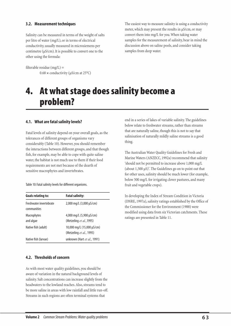
Volume 2 Common Stream Problems: Water quality problems 6 3
3.2. Measurement techniques
Salinity can be measured in terms of the weight of salts
per litre of water (mg/L), or in terms of electrical
conductivity, usually measured in microsiemens per
centimetre (µS/cm). It is possible to convert one to the
other using the formula:
filterable residue (mg/L) =
0.68 ´ conductivity (µS/cm at 25°C)
The easiest way to measure salinity is using a conductivity
meter, which may present the results in µS/cm, or may
convert them into mg/L for you. When taking water
samples for the measurement of salinity, bear in mind the
discussion above on saline pools, and consider taking
samples from deep water.
4.1. What are fatal salinity levels?
Fatal levels of salinity depend on your overall goals, as the
tolerances of different groups of organisms vary
considerably (Table 10). However, you should remember
the interactions between different groups, and that though
fish, for example, may be able to cope with quite saline
water, the habitat is not much use to them if their food
requirements are not met because of the dearth of
sensitive macrophytes and invertebrates.
4.2. Thresholds of concern
As with most water quality guidelines, you should be
aware of variation in the natural background levels of
salinity. Salt concentrations can increase slightly from the
headwaters to the lowland reaches. Also, streams tend to
be more saline in areas with low rainfall and little run-off.
Streams in such regions are often terminal systems that
end in a series of lakes of variable salinity. The guidelines
below relate to freshwater streams, rather than streams
that are naturally saline, though this is not to say that
salinisation of naturally mildly saline streams is a good
thing.
The Australian Water Quality Guidelines for Fresh and
Marine Waters (ANZECC, 1992a) recommend that salinity
‘should not be permitted to increase above 1,000 mg/L
(about 1,500 µS)’. The Guidelines go on to point out that
for other uses, salinity should be much lower (for example,
below 500 mg/L for irrigating clover pastures, and many
fruit and vegetable crops).
In developing the Index of Stream Condition in Victoria
(DNRE, 1997a), salinity ratings established by the Office of
the Commissioner for the Environment (1988) were
modified using data from six Victorian catchments. These
ratings are presented in Table 11.
Table 10: Fatal salinity levels for different organisms.
Goals relating to: Fatal salinity:
Freshwater invertebrate 2,000 mg/L (3,000 µS/cm)
communities
Macrophytes 4,000 mg/L (5,900 µS/cm)
and algae (Metzeling et al.,1995)
Native fish (adult) 10,000 mg/L (15,000 µS/cm)
(Metzeling et al., 1995)
Native fish (larvae) unknown (Hart et al., 1991)
4. At what stage does salinity become a problem?

Volume 2 Common Stream Problems: Water quality problems 6 4
High salinity is at best a catchment-scale hydrological
problem. At worst, it is a regional-scale issue. In short, it is
not something that can usually be successfully treated in
drainage lines alone.
Table 11. Salinity ratings for streams in Victoria. From (DNRE, 1997a).
Mountain Valley Floodplain Rating
< 34 mg/L (50 µS/cm) < 68 mg/L (100 µS/cm) < 68 mg/L (100 µS/cm) Ideal
< 102 mg/L (150 µS/cm) < 170 mg/L (250 µS/cm) < 204 mg/L (300 µS/cm) Close to ideal
< 204 mg/L (300 µS/cm) < 272 mg/L (400 µS/cm) < 340 mg/L (500 µS/cm) Moderately different to ideal
< 340 mg/L (500 µS/cm) < 476 mg/L (700 µS/cm) < 544 mg/L (800 µS/cm) Substantially different to ideal
> 340 mg/L (500 µS/cm) > 476 mg/L (700 µS/cm) >544 mg/L (800 µS/cm) Far from ideal
5. Possible solutions/treatments for salinity
Volume 2 Common Stream Problems: Water quality problems 6 5
Not surprisingly, there is a vast array of organic and
inorganic chemicals that find their way into streams where
they can potentially cause considerable problems for the
stream biota. These chemicals are grouped under the
general category of toxicants. The Australian Water Quality
Guidelines for Marine and Fresh Waters lists 18 inorganic
toxicants— mainly heavy metals—and many more
organic toxicants, including several pesticides, detergents,
and many chemicals used in industry as solvents,
chemical intermediates, and so on.
1.1. The natural state and how it has changed
Many of the inorganic toxicants are naturally found in
streams in very low quantities, coming mainly from the
weathering and erosion of various rocks and minerals.
However, there are many anthropogenic sources, including
mining waste, sewage and industrial effluent, the
combustion of fossil fuels (eg. beryllium and sulfur), street
run-off (eg. lead), photographic waste (silver), tanneries,
paper mills, chemical plants, gas works, waste
incineration, metal production and so on. Many of the
organic toxicants are manufactured chemicals, and so are
not naturally found in water in any concentration. These
chemicals enter the environment through various routes
such as industrial and manufacturing emissions and
discharges, run-off from agricultural land, municipal
effluents, and fuel combustion. In Victoria, one of the most
common toxicants in streams is mercury, due to its use in
gold mining.
TOXICANTS1. Introduction
The biological impacts of toxicants are too many to list
separately, but they range from a reduction in growth rate
and development, and pathological changes in gill, liver
and kidney tissue (salmonid fish response to chronic
exposure to ammonia), to impaired reproduction
(response of Daphnia to lead) and spinal deformities
(response of trout to lead) (ANZECC, 1992b). Some
chemicals, such as selenium and some pesticides, are toxic
to plants as well as animals. See (ANZECC, 1992a) for a
brief description.
2. Biological impacts of toxicants
3.1. Field characteristics
Because there is such a variety of different toxicants, there
is no easy generalisation to be made about how you
identify the effects of these chemicals, other than a lack of
aquatic organisms. Unless you have a particular reason to
suspect the presence of some toxicants (eg. a source such
as an urban or industrial drains, of mining effluent), your
first step should be to consider if water quality is actually a
problem.You should:
1. Search for the macrophytes, macroinvertebrates and
fish you would expect to find in a healthy stream.
2. If you don’t find any, look around and see if there is
suitable habitat and sufficient water for the animals
and plants you expect.
3. If there is suitable habitat, check other water quality
variables.
3. How do you recognise the presence of toxicants?
Volume 2 Common Stream Problems: Water quality problems 6 6
4. If none of these can explain the lack of life, talk to a
laboratory about testing for possible toxic chemicals in
your stream.
3.2. Measurement techniques
Measurement techniques vary for different toxicants.
Unfortunately, there are no easy field tests for these
chemicals as there are for the other water-quality
variables. Collection and analysis of samples for analysis of
toxicant concentration is complex. Tests for each chemical
will have different requirements for sample collection and
preservation. For many of these chemicals, there is a
variety of different methods for determining concentration,
which may arrive at different results. Seek professional help
if you suspect contamination with any of these chemicals.
The critical concentration depends on the chemical in
question. How toxic a chemical is may vary depending on
the pH and hardness of the water, and whether it is a
‘bioaccumulant’ (some chemicals will be absorbed by
animals, and not excreted, so they eventually accumulate
in the animal in much higher concentrations that the
surrounding water). For many chemicals, a suitable
threshold of concern is not known. See the ANZECC
concentration guidelines for further information.
Again this will depend on the chemical: seek professional
advice.
5. Possible solutions/treatments for toxicants
4. At what stage do toxicants become a problem?

OTHER BIOLOGICALPROBLEMS
• Other biological problems: an introduction
• Barriers to fish migration
• Large woody debris
• Stock management
• Rehabilitation for platypuses
• Rehabilitation for frogs

Volume 2 Common Stream Problems: Biological problems 6 8
In this section we discuss some of the problems, other
than water quality, that relate specifically to stream plants
and animals. We include some issues of habitat availability
(fish barriers and large woody debris), the effects that
domestic stock can have on streams, and the specific
requirements of some common flagship animals—
platypus and frogs.
OTHER BIOLOGICAL PROBLEMS:AN INTRODUCTION

Volume 2 Common Stream Problems: Biological problems 6 9
Fish, like other wild animals, exploit different parts of their
habitats to ensure the continued survival and success of
their species. Fish commonly spawn in one part of their
habitat, use a different part as a nursery area, and then
disperse into a third area for adult growth. Golden perch,
for instance, spawn during floods in lowland river reaches;
the young develop in floodplain or river margin nurseries;
then eventually travel upstream as juveniles. Murray cod
have recently been shown to make upstream spawning
migrations, using anabranches and flood-runners, then
returning to their original home territory. Each of these
habitat areas, plus free passage between them, is required
for the fish population to be sustained. Furthermore,
within adult growth habitats, each fish moves around to
feed within an area known as the home range. This
movement is needed for effective use of food resources;
preventing it is equivalent to shutting horses in a small
paddock—the food supply runs out.
The scale of these different movements varies greatly:
golden perch and silver perch can travel the length of the
Murray–Darling River system. Australian bass or eels may
migrate hundreds or thousands of kilometres to marine
environments to breed. Some small fishes such as
gudgeons and hardyheads, on the other hand, may
undergo life-cycle movements that extend only a few
kilometres, and thus are not so readily recognised as
‘migratory’. Other fish species fall between these two
extremes.
Most of Australia’s approximately 200 freshwater fish
species are considered to be migratory, and all of them
have some need to move between habitat areas within
streams (Harris, 1984; Mallen-Cooper and Harris, 1990;
Harris and Mallen-Cooper, 1994; McDowall, 1996).
BARRIERS TO FISH MIGRATIONBy John Harris* and Tim O’Brien
†
1. Introduction
There can be natural barriers to fish migration (eg. waterfalls,
sand slugs or zones of poor water quality) that could already
exclude native fish from upstream reaches. If such barriers
exist, then it would be a waste of resources to provide fish
passage across artificial barriers upstream of the natural
barrier.
What if migrations are blocked? Extensive declines in fish
populations in both coastal and inland drainage regions
have been linked to the obstruction of fish passage, among
other factors (Wager and Jackson, 1993; Harris and
Mallen-Cooper, 1994; McDowall, 1996). For both inland
and coastal species, obstructed fish passage has led to
many instances of declining populations or extinctions of
species from affected catchments.
Migration barriers interfere with the two main ecological
processes that sustain populations: recruitment and
growth. Population recruitment includes spawning, the
nursery phase, and juvenile dispersal into adult growth
habitats. Growth relates primarily to home-range feeding
activity, and may occur in pulses associated with the
seasons and with river-level rises. Another ecological
process is the dispersal of fish from drought-refuge areas
2. Effects of blocking migrations
* Fish biologist, 56 Alkaringa Rd, Miranda, New South Wales 2228. Ph: (02) 9525 2812, email: [email protected]
† Senior Biologist, Freshwater Ecology Division, Marine and Freshwater Resources Institute, PO Box 137, Heidelberg,Victoria 3084. Ph: (03) 9450 8633,
fax: (03) 9450 8730, email: t.o’[email protected]

Volume 2 Common Stream Problems: Biological problems 7 0
(such as remnant deep pools) into newly regenerated
habitats (for example, billabongs or previously dried-out
river channels) after rainfall and renewed stream flow.
Complete obstruction of migrations leads to local extinction
of some species (Harris and Mallen-Cooper, 1994). This
seems attributable mainly to blockage of the recruitment
migration of young fish, so that the upstream population
gradually ages and dies out. For example, populations of at
least four migratory coastal species disappeared from above
a small weir at Dight’s Falls in the lower Yarra River before a
fishway was installed. There are many similar cases. Less-
restrictive barriers such as low-level weirs, however, usually
allow some fish movement in periods of high stream flow.
Nevertheless, the obstructive effects of individual weirs in a
system are cumulative, and weirs are more insidious in their
effects than high dams. Movements are diminished rather
than prevented, and fish populations decline rather than
disappear. Home-range movements are interrupted.
Upstream migrating fish accumulate below the weirs while
waiting for suitable conditions for passage, where their
crowded populations suffer radically accelerated mortality
rates because of increased predation by the birds and
fishermen often seen congregating below weirs, because the
food supply is quickly used up, or because of disease in the
crowded conditions. Sampling of fish at the Torrumbarry
Weir on the Murray River showed that 98% of native fish
(mostly golden and silver perch) were located below the
weir wall at times of rising flow and temperatures.When a
fishway was built, thousands of native fish moved over the
weir, at rates of up to 700 per day (Anon, 1990).Without
building fishways or removing weirs, fish passage can occur
only infrequently, when weirs are inundated or ‘drowned-
out’ by high stream flows.
Barriers to fish passage are major limitations to stream
rehabilitation in any modified catchment (ie. most
catchments in Australia). Although the most obvious
barriers are large structures such as weirs, dams and
barrages, road culverts, fords, and even open shallow
stretches of water can block fish passage. A recently
completed survey by the Victorian Department of Natural
Resources and Environment gives an indication of the
magnitude of the problem. It found over 2,500 potential
obstructions to fish, including dams, weirs, culverts and
fords (O’Brien, 1997). In the streams of New South Wales,
there are 3,000–4,000 artificial barriers impeding fish
passage. A survey of 293 such structures in south-eastern
Australia by Harris (1980) found that less than 10% of
them had any provision for fish passage. Other studies
have questioned the effectiveness of existing fishways
(Russell, 1991).
Much of the literature describing work to overcome
obstacles to fish migration has come from the study of
salmonid species, which migrate upstream for spawning
when fully grown. Many Australian fish behave in the
opposite way, migrating downstream to spawn in
estuaries, juvenile fish making the journey upstream to
freshwater reaches. As well as the obvious size and
strength difference between juvenile and mature fish,
Australian native fish are not strong swimmers or jumpers
(compared with salmonids), hence barriers pose much
more of a threat to Australian native fish species than to
those of the northern hemisphere.
3. The extent of the problem
An important step in any rehabilitation design is to
identify barriers to fish passage. The things to look for are
extended stretches of shallow flow, perching or high drops,
and high velocity. Australian streams display huge
variability in stream flow, and many of our major
waterways are ephemeral systems. Even under natural
conditions there will be times when fish passage is not
possible. As a general stream rehabilitation design rule,
fish passage should be possible for 95% of flows. So when
identifying barriers, the minimum design flow is that
which is exceeded 95% of the time the stream is flowing (ie.
do not count the period when there is no flow). For many
ephemeral streams this means providing adequate
conditions for fish passage for only a few weeks per year.
4. Identifying barriers to fish passage

Volume 2 Common Stream Problems: Biological problems 7 1
4.1. High velocity
Generally, Australian fish have difficulty traversing long
stretches of uniform fast-flowing water. The preferred
solution is to provide roughness features such as boulders
which break up the current and provide low-velocity zones
for fish to rest and feed. High velocity areas are often a
feature of modified, smooth sections of streams like
culverts or fords. As a guide, there should be periods when
the flow velocity does not exceed 1 m/s and regular
(approximately every 1–2 m) low-velocity rest areas like
those provided by large rocks.
4.2. Shallow flow
Depending on their size, fish cannot pass through sections
of very shallow flow. Stream rehabilitation projects should
generally aim to have a ‘natural’ species composition,
thereby necessitating passage of all native fish. This
translates to a depth of at least 15 cm in smaller coastal
and headwater streams (O’Brien, 1997) (and deeper for
inland streams where some larger fish species are likely to
occur) for 95% of the time the stream is flowing.
4.3. Perching (around culverts)
A perched stream is one in which there is a drop or
waterfall that acts as a barrier to fish passage (refer to Full-
width structures, in Intervention tools, this volume, for
details on providing fish passage in such structures).
Culverts are common causes of stream perching.
Remember that for many smaller Australian fish species, a
drop of only 15 cm can be an insurmountable barrier.
Perching can be caused by downstream bed lowering, or
poor design of the culvert exit.
To solve the much larger perching problems created by
weirs requires the installation of fishways. The design of
concrete fishways is not covered in this manual, as these
structures can cost hundreds of thousands of dollars, and
are therefore beyond the means of stream rehabilitation
groups. (Contact the relevant water or conservation
department in your State for technical assistance if you
want to build one.)
4.4. Day migrant species
Culverts can pose another barrier to those fish which
migrate only during daylight. Some of these species will
not enter darkened tunnels. The only solution in this case
is to replace the culverts with fords.
4.5. Wide, shallow stretches of water
Wide, shallow stretches of water can be barriers to fish
because of depth or velocity as mentioned previously, or
through predation. Wide, shallow stretches of stream make
fish easy prey for birds. A series of rocks or logs placed in
the channel will provide cover, depth and low velocity to
allow easier fish passage.
There are several ways of overcoming barriers to fish
passage. The simplest is the rock ramp, a simple pile of rock
below the offending barrier that creates a gentle enough
water slope to provide fish passage. See Overcoming barriers
to fish passage, in Intervention tools, this Volume.
5. Techniques for creating fish passage

Volume 2 Common Stream Problems: Biological problems 7 2
The following notes on the management of large woody
debris (LWD, or snags) in streams are, in part,
summarised from the National Riparian Zone Guidelines
produced by LWRRDC (see the full document, with full
referencing, at www.rivers.gov.au).
It is now appreciated that LWD plays a crucial role in the
rehabilitation of Australian streams in humid regions. It is
clear that in many streams, especially the lowland
sand–clay streams that make up much of the length of our
perennial streams, snags are the single most important
habitat component. Set against this is the fact that a great
deal of effort has been directed at removing snags from
our streams over the last 150 years.
LARGE WOODY DEBRIS
1. Introduction
Key points aboutlarge woody debris• In streams with a mobile bed and deep water, LWD is
arguably the single most important habitat feature for
fish, algae and macroinvertebrates.
• Large volumes of LWD can increase flood stage, but the
effect of a single log is trivial.
• LWD can cause minor bank erosion.
• In almost every case, the ecological value of LWD far
outweighs the minor flooding and erosion problems
caused by the blockages.
• Removing further LWD from streams should be prohibited,
except in special circumstances.
• Artificially returning LWD to streams will be a critical part
of many stream rehabilitation projects until riparian
vegetation is able to supply sufficient material.
2.1. LWD and stream habitat
2.1.1. Woody debris as habitat for fish
Large woody debris provides important habitat for direct
use by a number of aquatic and terrestrial organisms.
Such uses include shelter from fast flows, shade, feeding
sites, spawning sites, nursery areas for larvae and juvenile
fish, territory markers and refuge from predators.
Snags are most effective as habitat if they have a complex
structure providing a number of different-sized spaces,
including hollows and spaces between branches. Branches
extending into the water column and above the water
surface provide habitat at the different water levels
required by different fish species. Single large trees that fall
into a river can often provide the full range of complex
spaces required.
Snags positioned at different locations within the stream
channel benefit different species. For instance, trout cod
(Maccullochella maquariensis) utilise snags that are located
in high-current zones towards the middle of the channel
and downstream of a bend. Murray cod (Maccullochella
peelii peelii), on the other hand, live around the bases of
snags in slower-flowing currents closer to river bends.
2. Biological and physical effects of LWD
Volume 2 Common Stream Problems: Biological problems 7 3
2.1.2. Snags as habitat for other organisms
In general, the types of snags that provide habitat for fish
also provide habitat for other aquatic and terrestrial
organisms. Submerged wood with a complex surface
structure of grooves, splits and hollows provides space for
colonisation by a range of invertebrates, microbes and
algae. Some invertebrates feed directly on the wood, while
others graze the biofilm (that is, the combined microbe
and algal community).
The species composition within the biofilm community
depends on the position of the wood substrate within the
water column. The shallower the water in which the wood
occurs, the higher the density of algal species. There are
fewer algae deeper in the water column where less light
penetrates.
Species composition of both biofilm and invertebrates also
depends on the character of the surface on which it forms
(the substrate). Snags of willows and other introduced tree
species appear to have a less diverse invertebrate community
than native/indigenous tree species (see Willow infested
streams, in Intervention tools, this volume). Similarly,
community composition varies according to the type of
substrate (for example, wood is better than a concrete pipe).
Birds, reptiles and mammals also use woody debris for
resting, foraging and lookout sites. Birds commonly use
the exposed branches of snags as perch sites, while turtles
often climb out onto the surface of snags. Snags spanning
the channel may also be used by mammals and reptiles as
stream crossing points. Many aquatic invertebrates have a
terrestrial adult stage and require snags extending above
the water surface to provide sites for their emergence from
the stream.
2.1.3. Snags as sites for carbon and nutrient processing
Another important—but often overlooked—function of
snags is their role in carbon and nutrient processing. Snags
provide important substrate for the development of biofilm.
The bacterial and fungal components of biofilm contribute
to the decomposition of the woody substrate and hence to
the supply of dissolved and particulate organic material
(carbon) to the water column. Organic matter is a major
source of food for invertebrates and fish. The algal
component of biofilm may also produce a significant
amount of food, through photosynthesis. Many invertebrates
and some fish, eat the algae that grows on wood surfaces.
The biofilm also readily transforms available nitrogen and
phosphorus by converting them to less-available
compounds. This has the potential to restrict nutrient
supply to nuisance algal and macrophytic growth.
In upland streams, large accumulations of woody debris
(debris dams) often span the entire channel. These retain
large amounts of particulate organic material. This
material decomposes into smaller pieces and is then
transported downstream. As stream size increases, large
debris dams become less common and the ability of
woody debris to retain these small particles may decrease.
Nevertheless, retention of organic material and
stabilisation of sandy substrate by snags may still be
significant in lowland rivers. Flow over snags also helps to
re-oxygenate the water and prevent stagnation which can
cause fish deaths, odours and other water quality
problems.
2.1.4 . The role of snags in habitat formation
As well as providing habitat for a range of aquatic and
terrestrial species, snags also contribute to the
development of other habitat types by their impact on
channel structure. The main types of habitat formed by
snags depend on snag orientation and stream power. Scour
pools formed by snags spanning the channel are
particularly important for wildlife, especially in streams
with low or no summer flow. When flow ceases these pools
provide the only habitat available for aquatic species, from
which animals can recolonise the rest of the river when
water level rises.
In sandy, turbid rivers where woody substrate may be the only
hard substrate available for colonisation, or in rivers that have
been isolated from floodplain organic food inputs by river
regulation and clearing, most of the food for aquatic animals is
found on snags.

Volume 2 Common Stream Problems: Biological problems 7 4
As well as providing habitat for stream organisms, woody
debris can have a significant effect on the stream itself, in
terms of erosion, and increased flood stage. Generally, for a
single piece of debris, these effects are so small that they
pose no significant threat to the stream as a whole but, as
described above, they may contribute to stream habitat. For
more information on the physical effects of snags, see
Management of large woody debris in Intervention tools,
this volume.
3. The physical effects of large woody debris on streams
There are two options available to increase the amount of
woody debris in your stream.
1. Revegetating the riparian zone will encourage the
natural recruitment of debris to the stream.
Unfortunately, this will take a long time, because the
vegetation has to mature to a stage where natural aging
leads to large branches or entire trees falling into the
stream. For example, silver wattle, a common small
riparian tree in south-eastern Australia, can fall into
the stream after only 30 years, while some eucalypts
probably do not begin to contribute large pieces of
debris to the stream until they are at least a hundred
years old.
2. The second option is to manually add wood to the
stream. This is discussed in Management of large
woody debris, in Intervention tools, this volume.
4. Managing large woody debris
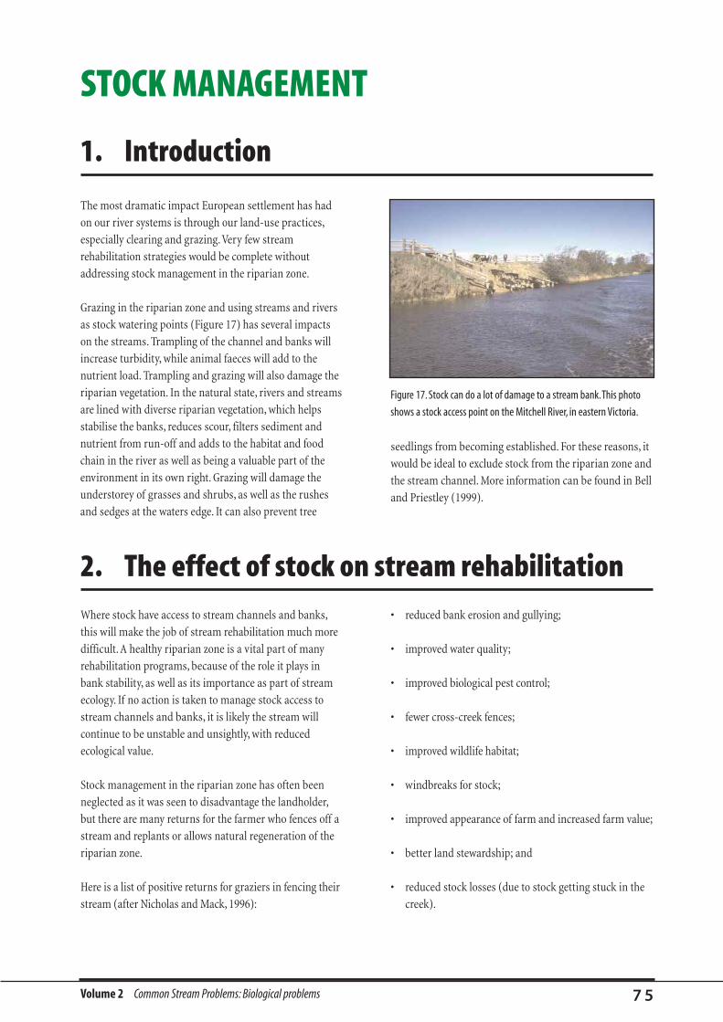
Volume 2 Common Stream Problems: Biological problems 7 5
The most dramatic impact European settlement has had
on our river systems is through our land-use practices,
especially clearing and grazing.Very few stream
rehabilitation strategies would be complete without
addressing stock management in the riparian zone.
Grazing in the riparian zone and using streams and rivers
as stock watering points (Figure 17) has several impacts
on the streams. Trampling of the channel and banks will
increase turbidity, while animal faeces will add to the
nutrient load. Trampling and grazing will also damage the
riparian vegetation. In the natural state, rivers and streams
are lined with diverse riparian vegetation, which helps
stabilise the banks, reduces scour, filters sediment and
nutrient from run-off and adds to the habitat and food
chain in the river as well as being a valuable part of the
environment in its own right. Grazing will damage the
understorey of grasses and shrubs, as well as the rushes
and sedges at the waters edge. It can also prevent tree
seedlings from becoming established. For these reasons, it
would be ideal to exclude stock from the riparian zone and
the stream channel. More information can be found in Bell
and Priestley (1999).
STOCK MANAGEMENT
1. Introduction
Figure 17. Stock can do a lot of damage to a stream bank.This photo
shows a stock access point on the Mitchell River, in eastern Victoria.
Where stock have access to stream channels and banks,
this will make the job of stream rehabilitation much more
difficult. A healthy riparian zone is a vital part of many
rehabilitation programs, because of the role it plays in
bank stability, as well as its importance as part of stream
ecology. If no action is taken to manage stock access to
stream channels and banks, it is likely the stream will
continue to be unstable and unsightly, with reduced
ecological value.
Stock management in the riparian zone has often been
neglected as it was seen to disadvantage the landholder,
but there are many returns for the farmer who fences off a
stream and replants or allows natural regeneration of the
riparian zone.
Here is a list of positive returns for graziers in fencing their
stream (after Nicholas and Mack, 1996):
• reduced bank erosion and gullying;
• improved water quality;
• improved biological pest control;
• fewer cross-creek fences;
• improved wildlife habitat;
• windbreaks for stock;
• improved appearance of farm and increased farm value;
• better land stewardship; and
• reduced stock losses (due to stock getting stuck in the
creek).
2. The effect of stock on stream rehabilitation

Volume 2 Common Stream Problems: Biological problems 7 6
Fencing off the riparian corridor does not mean ‘giving
up’ land. One of the main concerns for graziers who are
being urged to fence off their stream is that they do not
want to lose part of their land. Farmers can usually retain
the use of the ‘river paddock’ for selective gazing. The
basis for keeping stock away from the riparian corridor
for most of the time is to permit the natural regrowth of
native vegetation. Once the plants are well established, the
corridor can still be crash grazed during non-vulnerable
growing stages (when desirable plants are well
established, and not flowering) (Nicholas and Mack,
1996).
Managing stock access to streams requires that some form
of fence be erected around the riparian zone and, where
necessary, that alternative stock watering points
constructed. For information on this, see Managing stock
access to streams, in Intervention tools, this Volume.
3. Managing stock access
Volume 2 Common Stream Problems: Biological problems 7 7
Information used to prepare this section was sourced from
Tom Grant’s 1995 book The Platypus: a Unique Mammal
and Platypus Profiles (a series of information notes
produced by the Australian Platypus Conservancy). Expert
advice was also given by Mr Geoff Williams of the
Australian Platypus Conservancy, Melbourne.
Platypus (Ornithorhynchus anatinus) are so distinctive
that they need little introduction. They are an extremely
charismatic animal that can excite great enthusiasm for
conservation in local communities. Maintaining platypus
populations or encouraging the re-establishment of
platypuses in impacted streams can be an excellent goal
for a community rehabilitation project, as it can muster
wide community support for generalised improvements to
REHABILITATION FOR PLATYPUSESBy Kathryn Jerie and Tanya Rankin*
the stream and riparian zone. This can have positive
impacts on many other important aquatic values, such as
improved water quality, increased fish and
macroinvertebrate biodiversity, and the revegetation of
riparian zones. Community rehabilitation projects
focusing on platypuses can also succeed in improving the
visual appeal of a waterway and its value for recreational
users.
1. Introduction
2.1. Description and habit
The platypus is one of only two egg-laying mammals (the
other is the echidna). Platypuses are well adapted for their
aquatic lifestyle, and have a dense covering of dark brown
waterproof fur; only their webbed feet and distinctive,
duck-shaped bill are hairless. Male platypuses average 1.7
kg in weight and 50 cm in length, while females are quite a
bit smaller, weighing around 0.9 kg and are about 43 cm
long. They excavate burrows in earth and clay river banks,
burrowing at a rate of up to half a metre an hour. They
may spend as much as 17 hours a day asleep in their
burrows.
When diving for food, platypuses close their eyes, ears and
nostrils, and use their electro-sensitive bill to pick up tiny
electrical impulses from muscle contractions in their prey
which live in and among sediments and rocks on stream
bottoms. Their prey consists of a wide range of
macroinvertebrates, including worms, insects, molluscs
and crustaceans. Platypuses feed voraciously: it has been
estimated that they can eat up half their own bodyweight
in food each night. They come out of their burrows mainly
at night to forage in still pools in rivers, but can
occasionally be seen during the day, especially in the
morning.
2.2. Distribution
Platypuses are unique to eastern Australian watercourses
and are found naturally in and around many different
types of water body, from coastal rivers to reservoirs,
billabongs and highland streams in eastern Australia and
Tasmania. Platypuses are reasonably common and
widespread and so are not currently in any danger of
extinction. Numbers, however, have declined, particularly
in urban streams and in waterways in intensively farmed
regions. This is thought to be due to a number of
anthropogenic factors, the main ones being habitat
degradation, litter inputs to streams, and poor water
quality.
2. Biology of the platypus
* Institute of Wildlife Research, School of Biological Sciences, University of Sydney, NSW 2006. Ph: (02) 9351 3134, fax: (02) 9351 4119, email: [email protected]
Volume 2 Common Stream Problems: Biological problems 7 8
2.3. Life cycle
The platypus mating season is from about July to October,
with most mating occurring in September. The two to
three eggs produced are laid about one month after
mating, and hatch about 10 days after that. The young are
fed milk by the mother for about three and a half months,
after which the juveniles leave the nesting burrow and
begin to feed independently, first entering the water
between January and March. In late summer and early
autumn they leave their mother’s range to find territories
for themselves. During this time, they may occasionally be
found a considerable distance from the nearest waterway
as they move overland in search of new territories. At this
stage, young animals may be at great risk of being killed by
dogs or foxes.
Platypuses are long-lived animals. In captivity, some have
survived for over 20 years. In the Shoalhaven River, New
South Wales, Dr Tom Grant has re-trapped a female over
13 years after she was first captured, so platypuses can
potentially remain in the same area for a very long time.
Unfortunately, very little is known about rates of
population growth, how platypus go about finding new
habitat, or how many individuals are required for a
sustainable population.
3.1. Surveying for platypuses
If you want to know if you have platypuses in your stream,
you can get your community group to conduct a survey.
Surveys are usually visual, consisting of coordinated
observations of the stream at the times when platypuses
are most likely to be active. Other survey methods involve
capturing the animals in special nets. Netting is often
considered to be more conclusive than a visual survey, but
netting surveys can be conducted only by experts who are
trained and licensed by the relevant authorities. Only
visual surveys are conducted by community groups.
Visual surveys are quite simple and can be very effective.
They involve sitting quietly on the stream banks, with
minimal movement, and watching the stream for signs of
platypus activity. Observers should be stationed at regular
intervals, every 25 m or so, along likely-looking pools from
about an hour before dusk until it is too dark to see, or
from dawn for an hour or two. Binoculars can sometimes
be useful for these surveys. Platypuses can be identified by
their characteristic double splash duck-dive, and when
resting on the surface while they chew their food. The only
other animal that might be confused with the platypus is
the native water rat. Water rats can be readily
distinguished from platypuses as they usually have a white
tip to their tail, and ordinarily swim rapidly along the
surface between landmarks, such as rocks or logs jutting
out of the water. Platypuses dive frequently and, unlike the
water rat, are rarely seen resting on landmarks, spending
most of their time in the water. The swimming action of
water rats is also quite different from platypus swimming,
to the eye of an experienced observer. It doesn’t take too
long to become familiar with the distinctive swimming
and diving of platypuses. Don’t be disheartened if no-one
spots a platypus the first time out—try again a few weeks
later. Other native aquatic animals that may be seen during
these surveys are the eastern water dragon, long-necked
tortoises, and various water birds. Record observations
carefully (date, location, time, and number of animals
seen). This information can then be used for monitoring
platypus populations over time, which is particularly
important if stream improvement works are made. State
and local wildlife services are also often interested in the
results of these surveys, and usually appreciate the data
being passed on.
If your community group is really keen, radio-tracking
studies can also be conducted to identify burrow locations
and activity patterns of platypuses. These, however,
require considerable expertise, and involve the use of
specialised and very expensive equipment. Contact your
State wildlife service for further information.
3. Do you already have platypuses?

Volume 2 Common Stream Problems: Biological problems 7 9
4.1. Habitat for platypuses
Bank stability is very important to platypuses, because of
the need to have stable and secure burrows for resting and
breeding. Platypuses excavate burrows in the stream bank,
up to several metres long, where they may spend many
hours asleep each day. The burrows usually have domed-
shaped entrances which can be difficult to spot, under or
near the water surface or in undercut banks, usually where
there is dense overhanging riparian vegetation. Burrows are
often associated with tree roots along the waters edge. The
extensive roots of native trees like river red gums and
casuarinas provide structure and stability for the burrows,
preventing them from collapsing, especially during floods.
Revegetating the riparian zone with native endemic trees,
shrubs and sedges can help provide suitable burrowing
habitat for local populations or may encourage platypuses
to return to the area and will help stabilise eroding banks.
Remember, when seeking to stabilise banks, you should try
to avoid hard engineering techniques that can reduce
invertebrate habitat as well as remove suitable platypus
burrowing sites. The most platypus-friendly bank
stabilisers are native endemic trees with extensive root
systems, with an understorey of smaller shrubs and sedges.
4.2. Platypuses and willows
In the past willows have been used to stabilise stream
banks but these days, for environmental reasons, willow
planting is discouraged. Platypuses often excavate their
burrows amongst willow roots, but the benefits the trees
provide are outweighed by the damage they cause through
choking stream channels, slowing or otherwise altering
stream flows, and increasing sedimentation of pools.
Macroinvertebrate communities are also affected by over-
growth of willows. The Australian Platypus Conservancy
has been conducting a study on the effect of willow
eradication on platypuses in Diamond Creek and the Yarra
River, Melbourne. In the study, willows were killed but
their stumps and roots were left in place to maintain bank
stability and prevent collapse of platypus burrows. Though
the study is still incomplete, animals monitored by
radiotracking behaved in a normal manner during willow
removal, and later continued to use the burrows associated
with the dead willow roots. More than two years on,
platypus densities in the cleared reach were the same or
possibly higher than before the willow eradication
program began. It seems from this study, that willow
eradication is not likely to drive platypuses from the reach
if the stumps and roots are left in place and disturbance to
stream banks is minimised. Eventually, removal of willows
will allow streams to return to their natural flow regimes,
reduce sedimentation of pools, and allow stream
macroinvertebrate communities to increase and diversify.
Willow eradication may act to encourage platypus
populations, but remember that bank stabilisation and
revegetation with native plants are of utmost importance
to maintain and improve platypus habitat.
4.3. Platypuses and flow regulation
A good riffle-pool-riffle sequence is also important in
streams, as it provides a range of flow regimes which
encourage diverse and abundant macroinvertebrate
populations, which the platypus need to eat. Channelised
stream reaches may need extra attention to re-create these
diverse flows. Regulation of rivers may also pose problems.
Although platypuses are often found in and below artificial
impoundments they are not usually found in waters deeper
than several metres—it is thought that this is because their
macroinvertebrate food supply is restricted at these depths.
Flow regulation can also threaten long-term survival of
platypus populations in other ways. Firstly, where water use
extends the extreme low-flow periods, this may prolong
drought stress and reduce the food supply of the
platypuses. Secondly, impoundments may reduce the
frequency of scouring flows, resulting in increased
sedimentation and reduction of pool habitat downstream
of the dam. Long-term studies on the Shoalhaven River in
New South Wales have suggested that platypuses are
sensitive to sedimentation of pools when environmental
flows are inadequate to scour and flush sediments
downstream. In addition, a wire mesh cover (mesh less
than 8 cm2) should be fitted over all intake pipes to prevent
water pumps killing or injuring animals.
4.4 . Macroinvertebrates and hunting
When hunting, platypuses turn over rocks and stir up
sediments in the stream bottom with their strong webbed
forefeet, and quickly snap up any macroinvertebrates they
4. Habitat requirements
Volume 2 Common Stream Problems: Biological problems 8 0
sense. Therefore, habitat that encourages
macroinvertebrates is always beneficial to platypuses. For
example, re-creating riffle habitats, replacing woody
debris, and increasing hydraulic diversity can improve
conditions for macroinvertebrate communities, which in
turn are the food supply of platypuses.
4.5. Area of suitable habitat required by platypuses
Unfortunately, the total area of suitable habitat required to
support a permanent platypus population is not well
known. It depends on combinations of characteristics such
as the width and depth of the stream, flow rates,
macroinvertebrate production rates, the availability of
suitable burrow sites, and even the risk of predation by
dogs and foxes. Platypuses can have large overlapping
home ranges: females use about one to two kilometres of
stream, while males may patrol up and down six to seven
kilometre long stretches of stream. In fact, some male
platypuses have been shown to move several kilometres in
a single night. It is therefore suggested that up to ten
kilometres of quality habitat is needed in a wide stream,
longer for narrower streams, to maintain healthy platypus
populations. If this seems daunting, remember that any
improvement will be beneficial to platypuses, no matter
how small it may seem, particularly if improvements are
maintained and added to over time.
5.1. Water quality issues
Platypuses are not directly affected by many water quality
issues such as turbidity, dissolved oxygen, and nutrient
loads. Platypuses are more likely to suffer indirectly as a
result of decreases in water quality if these, in turn, reduce
the quantity and diversity of macroinvertebrates. Because
of this, any management to improve the diversity and
abundance of macroinvertebrate populations has the
potential to encourage platypuses.Very high levels of
turbidity, low dissolved oxygen, high nutrient and
pollution levels, and low pH can all have detrimental
impacts on macroinvertebrate communities. These
problems can often be difficult to tackle, as many stream
inputs have diffuse sources. Some improvements that can
be made include increasing the size of riffles, which will
help to oxygenate the water, and restoring and maintaining
riparian buffer strips that will filter some of the sediment
and nutrients from run-off. Reducing nutrient loads will
also serve to reduce the risk of algal blooms—some algal
blooms are potentially toxic, but the effect of these on
platypuses has not yet been investigated.
Though platypuses are less directly affected by poor water
quality than macroinvertebrates or fish, in Tasmania
recent research has implicated the influence of poor water
quality (especially elevated levels of faecal contamination)
on the incidence of a fungal infection in a few localised
populations of platypuses. This disease has not yet been
found in mainland platypus populations, but its
occurrence suggests that good water quality may be more
directly important to platypus than previously thought.
5.2. Litter and refuse problems
Platypuses are affected by litter and refuse in streams.
There have been many reports of badly injured or dead
animals found tangled in discarded fishing line, beer
packaging, and similar coarse plastic litter. This is an
important problem in urban areas—recent platypus
surveys in urban Melbourne have found up to 10% of
animals were fouled by some or other extraneous material.
Many of the animals had severe injuries as a result; some
were so badly injured they had to be euthanased.
Platypuses are also drowned in illegal eel nets and in
yabbie traps if they are left unattended and improperly set.
Clean-up days and the use of litter traps can greatly reduce
litter problems for platypuses.
5. Water quality requirements

Volume 2 Common Stream Problems: Biological problems 8 1
• It is not known how likely it is that platypuses will find
a newly rehabilitated site a considerable distance from
current populations. For this reason, if you wish to
increase platypus populations in your area, it is
probably best to start restoration work up or
downstream from a known population. Be sure your
improvement work does not disturb platypuses while it
is in progress.
• A well-vegetated riparian zone is important to
platypuses, as it provides cover from predators, and
contributes to stabilisation of banks for suitable
burrowing sites. Native vegetation is preferred for
stream macroinvertebrates as they are better able to
process native leaf litter compared with introduced
trees and weeds. Diverse and abundant
macroinvertebrate communities are important to
platypuses as their food supply.
• Platypuses travel considerable lengths of stream during
their nightly foraging and territorial patrolling. To
maintain platypuses, you may need well over six
kilometres of suitable habitat, depending on stream
depth, width and other factors previously discussed.
• Rubbish in the stream is possibly the most important
aspect of water quality to affect platypuses directly. It is
important to keep the stream free of potentially fatal
rubbish, such as fishing line, beer packaging, wire and
other rubbish. Also ensure there is community
education about the dangers of badly set yabbie traps
and illegal eel nets.
• Indirectly, water quality can affect platypuses. It is vital
to have a good macroinvertebrate population as food
supply for the platypuses. If poor water quality
prohibits this, problems must be addressed before you
can expect to support platypuses in your stream.
• Intake pipes for water pumps may suck in and kill
platypuses. To prevent this, wire mesh covers (mesh
less than 8 cm2) should be fitted over all intake pipes.
• When doing instream works in areas known to support
platypuses, try to avoid working between the breeding
and rearing season (August to March) when damage to
the burrow could be fatal to young animals. At the very
least, attempt to identify areas of suitable burrow
habitat and important foraging areas, and avoid
excessive disturbance to these sites.
• Try to keep disturbances of the stream minimal in
known platypus areas. If extensive works are planned,
consider staging the works so that no more than a 500
metre stretch of stream bank is disturbed in any one
year.
• Shallow riffles that are too long can expose platypuses
to predators; alternating sequences of pools and riffles
are preferred in riverine habitats.
6. Rehabilitation tips
For those who are interested in reading more about this
remarkable animal, we recommend Tom Grant’s excellent
book The Platypus: a Unique Mammal (1995, UNSW Press
Ltd, Sydney).
7. Further reading

Volume 2 Part 1: Common stream problems: Biological problems 8 2
Amphibian ambassadors such as Kermit and Tidalik have
raised the community awareness of frogs to a point where
they adorn almost as many T-shirts as whales and
dolphins. Popularity of this magnitude can be very useful
when you are trying to focus a community upon the task
of stream rehabilitation.
Frogs are commonly found near slow-moving, or stagnant
water bodies, from the backwaters of rivers to lakes,
ponds, waterholes and billabongs.
REHABILITATION FOR FROGSBy Fleur Bound
1. Introduction
You can check to see if you already have frogs by listening for
calls, spotlighting at night or searching typical hiding places
during the day. Most frogs are active during the warmer
spring and summer months in the evening or after rain.
You can identify frogs from their calls. Use a hand-held
tape recorder to record calls and compare these with
commercially recorded calls. The calls can also be used to
locate frogs, so they can be identified visually. When
locating frogs by their calls, a technique of triangulation
requiring two people is invaluable. The two people stand a
few metres apart and each aim their torch in the direction
they think the sound in coming from. The frog will be
located where the two beams cross.
It is also possible to locate inactive frogs by day. Most
species shelter in damp places close to water; ie. under
logs, rocks or old fence posts (remember to replace the
shelter), in drains and water tanks; even on occasion in
rain gauges and public toilets.
Identifying frogs is best done by experts, but if you just
want to capture, identify and release them, it is important
to handle frogs carefully. Their skin is delicate, and dries
out easily, so you should always have wet hands when you
touch them. Grab your identification book and attempt to
identify the frog. A good text to start with is:
Barker, J., Grigg, G.C., Tyler, M.J. (1995) A Field Guide to
Australian Frogs. Surrey Beatty & Sons Pty, Ltd.
According to Barker et al. (1995), it is still possible to
discover new species, especially in remote areas.
2. Do you already have frogs?
Because they are amphibious, frogs have two sets of
habitat requirements: one aquatic, and one terrestrial.
While frogs require some rainfall to survive, they are not
totally dependent upon permanent freshwater bodies
(Tyler, 1994). In fact, most Australian frogs breed in
intermittent bodies of water, but time their life cycles so
that their tadpoles (which cannot live without water)
have developed legs and can leave the water holes before
they dry up.
Arid areas have highly variable rainfall, making them the
least hospitable environment for frogs. However, some
frogs can still be found in the arid areas of Australia. These
frogs survive by burrowing in the soil to a depth where it is
cooler than the surface and where moisture is retained.
Desert burrowers, as they are referred to, require soils they
can dig in (Tyler, 1994).
Most frogs prefer slow-moving water bodies, and are
commonly found in backwaters and billabongs. They are
3. Habitat requirements
Many species of frog rely heavily upon the temporary
water bodies provided by the inundated floodplain. These
habitats occur less frequently with river regulation, and in
some cases have disappeared altogether.
Volume 2 Common Stream Problems: Biological problems 8 3
most dependent upon aquatic habitat while breeding and
as tadpoles, as these stages of the life cycle are spent
submerged.Very few species of frog can tolerate saline
water, so if you are in an estuarine region, or your river is
naturally salty, you should not expect to find too many
frogs.
The terrestrial habitat requirements of frogs include plenty
of dense riparian or marginal vegetation. This helps frogs
avoid predators, and also reduces the desiccating effects of
the sun on the frogs delicate skin. Frogs also utilise woody
debris and large rocks as shelter from desiccation and
predation. A diverse terrestrial habitat will also make a
larger range of invertebrates (such as insects) available for
frogs to eat.
Habitatrequirements of frogs:• a consistent source of moisture;
• water for breeding;
• places to shelter from predators and drying out; and
• fresh, rather than saline, water.
Frogs generally locate food by sight. They capture prey on
their long sticky tongues. When they sense movement, the
tongue is flicked far forward so that the top surface lands
upon the prey, which is then drawn into the stomach. This
entire process occupies a fraction of a second. Almost all
frogs have small teeth, but these play a minor role to the
tongue, and are only used for gripping larger prey until the
tongue can gain control of it.
Most frogs feed out of water, as an adhesive tongue is of
little use under the water. Those species which do feed in
water usually lunge at their prey with jaws open and use
their front legs to stuff the prey into their mouth.
Numerous factors influence the range of prey consumed,
significantly the habitat and season, but a frog’s diet also
depends on its size. Larger species of frogs tend to
consume large prey (such as grasshoppers and even other
frogs), while small species tend to consume smaller prey
(such as ants and other insects). Tadpoles usually eat algae
and detritus.
4. Food and hunting
Flow regulation can affect frog populations by eliminating
suitable habitat and by altering flow regimes and water
temperatures downstream that may be critical for the
survival and growth of eggs and larvae (Watson et al. 1991).
5. Flow regulation
Following courtship, males and females couple, and the
male fertilises spawn as it is laid. Where and when this
spawn is laid can help to identify the frogs involved. The
spawn develop into tadpoles which eventually
metamorphose into frogs. The amount of time it takes for
a tadpole to mature to a frog can vary from as little as a
couple of weeks, to as much as a year.
6. Life cycles
Volume 2 Common Stream Problems: Biological problems 8 4
Frogs are very sensitive to environmental change, and
declining populations in your area may therefore indicate
water quality degradation. Monitoring frog populations in
some situations has the added potential of indicating the
presence of contaminants in water systems thereby
alerting people to possible human health and livestock
hazards (Rauhala, 1997).
The aquatic environment can be polluted with a variety of
chemical substances, the most common being heavy
metals, insecticides, herbicides and fungicides. The effects
of these upon frogs is covered in detail in Tyler (1994).
Common malformations in frogs that can result from
these chemicals include extra limbs that can be either
functional or dysfunctional, the absence of one or both
eyes, a failure of the lower jaw to grow at the same rate as
the upper jaw and one limb that grows to half the normal
size.
Many of these contaminants can be controlled by changing
the way the original chemicals are used. Reducing the
amount of chemicals you use, applying them directly, and
avoiding spraying them directly onto riparian vegetation,
can all reduce their impact on frogs.
7. Water quality
In summary, the following considerations are important
when rehabilitating for frogs:
• Restrict stock access to the stream to allow vegetation
to grow and to minimise compaction of soil on the
stream bank. This will also allow the development of a
thick riparian zone which will provide habitat for frogs,
and their prey.
• When placing rehabilitation structures, place logs and
other structures in positions that will provide shelter
for frogs during the day from predation and the sun.
• Areas of slow flow are essential for frogs to breed.
These can be instream, but they are more commonly on
floodplains, or in temporary water bodies.
• A wire mesh cover should be fitted over all intake pipes
to prevent frogs and other wildlife from being sucked in.
• Good water quality within the stream, and in adjacent
temporary water bodies is essential for tadpoles to
mature enough to become frogs.
• Minimise herbicide, insecticide or fungicide spraying
near stream banks, and in any areas that may provide
habitat for frogs. Their highly permeable skins make
them very susceptible to chemicals in the water and on
riparian foliage.
8. Rehabilitation tips

PART 2:PLANNING
TOOLS
NATURALCHANNEL DESIGN
• Catchment review: developing a catchmentperspective and describing your stream
• Designing a more natural stream
• Empirical approaches to designing a naturallystable channel
• Channel evolution approach to rehabilitationdesign
• Predicting the scour produced when you putthings into streams
• How changing the channel can affect flooding

While the focus of most stream rehabilitation projects is
limited to a particular reach of a stream or river, it must be
remembered that this reach does not exist in isolation
from its upstream catchment. The catchment land use, and
the processes of run-off and groundwater flow, help to
determine the character of the river. Whatever happens in
the rehabilitation reach will have an effect on the reaches
downstream. Also, conditions downstream will determine
the potential for migration of fish into the rehabilitation
reach. Lowland rivers cannot be considered in isolation
from their floodplains, which perform various functions
such as storage of flood waters, provision of food supplies
for organisms that live in the stream, and provision of
habitat for species that need access to floodplains to
complete their life cycle.
It is impossible to manage entire catchments without
dividing them into manageable units. Defining these units
is essentially a classification exercise. By classifying the
stream into reaches, or groups of reaches, we are really
saying that each reach of the stream is more similar to itself
than it is to the next reach up or downstream. This means
that reaches can be used as planning units, allowing
management effort to be more effectively distributed.
This section discusses one approach to doing this
classification. Step 5 of the procedure emphasises that
priorities should be set at progressively smaller scales,
from catchments down to reaches, and then to problems
within reaches. We propose the following hierarchy of
management units for rehabilitation planning:
catchments; sub-catchments; segments; groups of reaches;
and reaches.
One of the most important tasks in river management is to
gain an understanding of the rehabilitation reach from the
catchment perspective. This is done by undertaking a
catchment-scale investigation. There are many forms a
catchment review can take, such as a drive through the
accessible parts of the catchment, walking and observing
the entire length of stream, examining topographic maps,
or detailed monitoring and recording of stream variables
on a geographical information system (GIS).
The first task is to divide the stream into manageable units
that will form the basis of planning. This is not a trivial
task.
Volume 2 Planning Tools: Natural channel design 8 7
In Step 3 of the Stream rehabilitation procedure (How
has your stream changed since European settlement?)
(Volume 1) you were asked to describe and
characterise your stream. This section of the manual
provides more detailed information on the tasks that
were described in Steps 3 and 4. Step 3 had four tasks:
• Task 1: Divide the stream into management units (eg.
segments and reaches)
• Task 2: Construct a template of the rehabilitated channel
• Task 3: Describe the present stream condition
• Task 4: Map the condition
In this section we provide more guidance on completing
Tasks 1–3 of Step 3 as well as some information on
assessing the interactions between reaches. Finally we
provide some extra information on identifying the main
problems in a reach for Step 4.
CATCHMENT REVIEW:DEVELOPING A CATCHMENT PERSPECTIVEAND DESCRIBING YOUR STREAM
1. An introduction to catchment review
2. Dividing the stream into manageable units (Task 1 of Step 3)
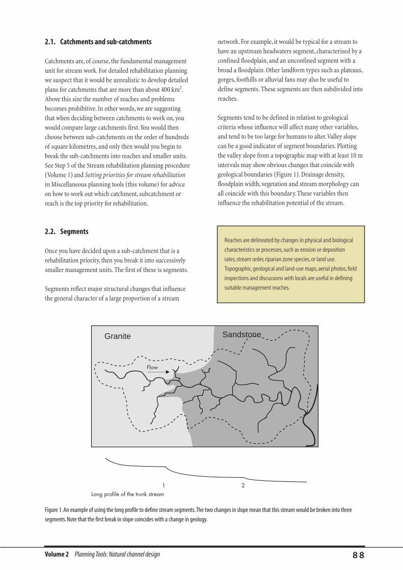
Volume 2 Planning Tools: Natural channel design 8 8
2.1. Catchments and sub-catchments
Catchments are, of course, the fundamental management
unit for stream work. For detailed rehabilitation planning
we suspect that it would be unrealistic to develop detailed
plans for catchments that are more than about 400 km2.
Above this size the number of reaches and problems
becomes prohibitive. In other words, we are suggesting
that when deciding between catchments to work on, you
would compare large catchments first.You would then
choose between sub-catchments on the order of hundreds
of square kilometres, and only then would you begin to
break the sub-catchments into reaches and smaller units.
See Step 5 of the Stream rehabilitation planning procedure
(Volume 1) and Setting priorities for stream rehabilitation
in Miscellaneous planning tools (this volume) for advice
on how to work out which catchment, subcatchment or
reach is the top priority for rehabilitation.
2.2. Segments
Once you have decided upon a sub-catchment that is a
rehabilitation priority, then you break it into successively
smaller management units. The first of these is segments.
Segments reflect major structural changes that influence
the general character of a large proportion of a stream
network. For example, it would be typical for a stream to
have an upstream headwaters segment, characterised by a
confined floodplain, and an unconfined segment with a
broad a floodplain. Other landform types such as plateaus,
gorges, foothills or alluvial fans may also be useful to
define segments. These segments are then subdivided into
reaches.
Segments tend to be defined in relation to geological
criteria whose influence will affect many other variables,
and tend to be too large for humans to alter.Valley slope
can be a good indicator of segment boundaries. Plotting
the valley slope from a topographic map with at least 10 m
intervals may show obvious changes that coincide with
geological boundaries (Figure 1). Drainage density,
floodplain width, vegetation and stream morphology can
all coincide with this boundary. These variables then
influence the rehabilitation potential of the stream.
Reaches are delineated by changes in physical and biological
characteristics or processes, such as erosion or deposition
rates, stream order, riparian zone species, or land use.
Topographic, geological and land-use maps, aerial photos, field
inspections and discussions with locals are useful in defining
suitable management reaches.
1 2Long profile of the trunk stream
Flow
Figure 1. An example of using the long profile to define stream segments.The two changes in slope mean that this stream would be broken into three
segments. Note that the first break in slope coincides with a change in geology.
Granite Sandstone

Volume 2 Planning Tools: Natural channel design 8 9
2.3. Defining reaches
A reach is the basic stream management unit. It represents
a length of stream with reasonably uniform
characteristics, and might vary in length between a
kilometre and tens of kilometres. In practice, the reach can
be defined on the basis of many criteria (Table 1)
including physiography, bed material, discharge, riparian
vegetation and aquatic organisms (species present) (eg.
Figure 2). Reaches can also be defined in relation to point
impacts such as dams or sewage-treatment outlets, if these
are important to your management objectives.
The transition from one reach to the next may not be clear,
so defining the start and finish of reaches is a subjective
process (except where major abrupt changes take place
like a dam or change of stream order). There is no hard
and fast rule about how long a reach should be. The main
principle is to make sure they are of a manageable size. For
example, a 40 km reach running through many properties
may be difficult to manage.
Most larger catchments in Australia have gone through
some form of catchment review. The responsible
administrative authorities are usually familiar with the
catchment. They should be consulted to help with this
process of dividing the catchment into management
reaches. The normal procedure for selecting reaches is to
initially define them from maps and aerial photographs,
then check them for uniformity in the field.
2.4. Stream groups
Reaches are the traditional unit of management for
streams, and they are easy to define in larger streams.
However, most of the length of the stream network is
comprised of smaller streams rather than the bigger ones
that are the traditional target for management. A stream
network is usually a bifurcating (ie. tree-like) network.
Streams of different sizes are described as ‘orders’, with
two of the smallest streams with no tributaries (1st order
streams) joining to produce a 2nd order stream, two 2nd
order streams joining to produce a 3rd order stream, and
so on. Most larger Australian catchments would contain up
to a 5th or 8th order stream. A rule of thumb is that there
are 3 to 5 times as many streams of one order as the next
higher order (Strahler, 1964). The implication of this is
that for every 4th order stream that you define a reach for,
there might be 16 2nd order and 66 1st order streams. If
we call each of these small streams a ‘reach’, there would
Table 1. Criteria for defining reaches.
Area Examples of criteria
Floodplain Slope.
Confinement (floodplain width).
Anabranches/avulsions.
Channel Boundary materials (bedrock, boulder, gravel, sand, silt, clay).
Sinuosity of planform.
Size (as a general rule, a new reach is defined when the discharge changes by about 10%).
Shape (wide and shallow, or narrow and deep).
Tributary junctions.
Land use Urban, farming (grazing or cropping), or forest.
Vegetation Grass, willows, or native vegetation.
Biology Presence of important species (eg. endangered species, or distinctive species such as platypus).
Hydrological discontinuities Dams, weirs, major points of water abstraction or input.
Administration National Park, State Park, or different local governments.
Dividing your streams into manageable units requires a
classification.Within a catchment, streams can be classified
into segments, which can be subdivided into reaches. Smaller
streams can be grouped.
The River Styles approach (Brierley and Fryirs, 1997; Brierley,
1999) provides a methodology for classifying streams based
on physical criteria.

condition of the stream reaches. In other words, the group
of streams becomes a card in the Reach priority shuffle (see
Setting Priorities in the Miscellaneous tools section of this
volume). Note that when the group of streams is allocated
a priority in the priority shuffle, you will then have to go
through the priority procedure again for all of the streams
included in the group. This helps you to decide which
streams to work on first.
be an unmanageable number of reaches, and we probably
could not inspect them all anyway.
So, how do we classify all of these streams for
rehabilitation? The answer is to define reaches as far up
the stream network as you can before the number of
reaches gets unwieldy (perhaps 20 reaches would be an
upper limit). Upstream of this point you group the smaller
streams based on their similarity. For example, you might
note that all of the 3rd order streams on the granite
portion of the catchment are very similar in form and
condition. So these might become Group G2 streams (the
name is up to you). Cleared streams in this group might
become Group G2c streams, and so on. When it comes to
the prioritisation step (Step 5 of the Procedure) you can
compare the condition of the stream groups with the
Volume 2 Planning Tools: Natural channel design 9 0
SEGMENT 2
SEGMENT 1
A
B
CD
E
F
SEGMENT REACH BASIS FOR DEFINITION
1 The headwaters segment, characterised by a steep slope, a single channel and small floodplain
A Immediately below the dam, grazing on riparian zone
B State forest with good riparian vegetation
2 The floodplain segment, with a gentle slope, wide floodplain and multiple channels in one reach
C Floodplain widens out, anabranches develop
D Tributary junction, 10% increase in size
E Very similar to D, split to maintain a manageable length
F Sewage outfall, rumours of high nutrient status
Dam
Figure 2. An example of how you go about dividing a stream into segments and reaches.
Volume 2 Planning Tools: Natural channel design 9 1
Task 2 of Step 3 of the Stream rehabilitation procedure is
to construct a template of what the target stream should
ideally be like. This template is based on a combination of
information.
• A historical reconstruction of its condition before the
major disturbance.
• A nearby reference reach that is undisturbed. (In
general, the more your reach differs from the reference
reach in terms of cross-section, size and shape,
planform, substrate, vegetation and water quality, then
the worse its condition.)
• Established criteria. (These exist for water quality, and
in some areas the expected assemblages of
macroinvertebrates or fish are known.)
• General models of a desirable stream condition (eg.
perhaps in order to have high species diversity, the
stream in the area of interest should have a pool–riffle
sequence, and continuous stands of native vegetation
along the banks).
• Known empirical relationships (eg. measures of
channel width against catchment area may suggest that
the target reach is unusually wide).
You should develop the template by grouping all of the
above information.You then compare the template with
the existing condition, and look for assets, degraded assets
and problems that threaten those assets. Assets are
components of the present condition that closely resemble
the template (that is, they are close to ideal). Degraded
assets are features that no longer closely resemble the
template. Problems are features or processes that threaten
to degrade assets, or have already damaged degraded
assets. Once you have identified these components of the
stream, you can decide which features of the stream need
to be protected, and which need rehabilitation. Complete
rehabilitation is often not possible, because many of the
differences between the template and the present
condition may be irreparable.
Another way of thinking about the template is in terms of
developing an idea of the ecological potential of a
stream. Ecological potential is the expected condition of the
stream if it was unaffected by undesirable disturbances.
These disturbances are usually taken to be the large-scale
impacts that occurred after European settlement, some of
which may have ceased and some of which may still be
operating. Even when a disturbing activity has ceased
(such as mining) its legacy (sand slugs) may remain as a
major stream disturbance. Streams also suffer major
natural disturbances, such as might result from major
floods, droughts, landslides or avulsions. One important
difference between human and natural disturbances is that
human disturbances were often undertaken with the
intention of altering the stream to a desirable condition
that could be maintained, whereas after a natural
disturbance the stream might recover to its previous state,
or perhaps shift to another condition. These days, natural
disturbances are superimposed on human disturbances,
and this may change their impact. For example,
catastrophic floods may cause more serious changes in
channel morphology if the riparian vegetation has been
removed or replaced by less-dense or less-robust species.
For further information on developing the template see the
section How to design a more natural channel.This section begins
with ways to find historical information, as well as methods for
using nearby ‘reference’ reaches. Note that, in practice, you will
probably develop your template at the same time as you
describe the present condition of the stream.
Remember, the key is to look for assets, degraded assets,
and threats to those assets. The aim is not to simply
catalogue human damage to the stream.
3. Developing a template of the stream condition (Task 2 of Step 3)

Volume 2 Planning Tools: Natural channel design 9 2
At this stage you have divided the stream into sub-
catchments, segments, reaches, and reach-groups.You have
developed a template of what the stream could be like
(Task 2). Now it is time to describe the present condition of
your stream.
It is important to remember that ‘condition’ is a highly
subjective concept. Stream condition can be assessed
only relative to some arbitrary benchmarks.
Establishment of benchmarks involves application of
value judgments, such as that native species are superior
to exotic species, high diversity is better than low
diversity, an unregulated flow regime is better than a
regulated flow regime, stable channels are more desirable
than unstable channels—all these are human constructs!
Again, remember that we are interested here in the
natural assets of the stream, not simply in a catalogue of
perceived damage. Something is only a problem if it
threatens or damages a natural asset, or stops a
natural asset from recovering.
This section describes some existing methods that you
could use to assess the condition of your stream.
4.1. What variables to use
As described in Step 3: How has your stream changed since
European settlement? of the Stream rehabilitation process,
Describing reach conditionThe purpose of the following three sections is to describe the condition of a stream reach, and the impact of that reach on reaches up and
downstream.This can best be thought of in relation to Figure 3 below.The condition of the stream should be described in terms of the bed and
banks (in-channel), and the riparian zone, including point impacts.Then you must consider what is entering the reach from upstream and
downstream. Finally, you consider what is leaving your reach and affecting reaches up and downstream. By doing this you are really carrying out
a whole of catchment assessment of the stream condition.
4. Describing the condition of the reaches(Task 3 of Step 3)
Figure 3.The impacts of the catchment and up- and downstream condition on a reach.The photo on the right shows turbid water from a tributary entering
a stream with better water quality (Tarago River, Gippsland).
Riparian zone
Riparian zone
Inputs andoutputsupstream
FLOWDIRECTION
Inputs andoutputs downstream
Condition inthe reach

Volume 2 Planning Tools: Natural channel design 9 3
Volume 1, ideal stream rehabilitation projects will
routinely describe the condition of the following:
1. The diversity and populations of animals and
plants, as well as whole stream communities (eg.
platypus, fish, macroinvertebrates, macrophytes).
2. Riparian vegetation (diversity, structure (eg. forest or
grassland), weed invasion, natural).
3. Flow regime (flow duration and magnitude, any
regulation or water diversion).
4. Longitudinal connection along the river (artificial
barriers to movement of water, sediment and
organisms along the stream, eg. dams, diversions,
weirs, willow encroachment).
5. Lateral connections across the floodplain
Connection of the stream with the floodplain, including
billabongs and anabranching channels. (Things that
change lateral connectivity include levees, channel
enlargement, channelisation, changes to flow regime,
blocked flood channels, connection with billabongs.)
6. Water quality (turbidity, nutrients, oxygen, salinity,
temperature, toxicants).
7. Structural complexity and stability in the channel
(size of the channel, sediments, large woody debris).
Table 2. Possible approaches to describing the condition of the stream.
Measure Examples
Visual description of presence or absence "Native vegetation was absent from the reach, with willows being the only species
at one point in time. present."
"The water looked turbid."
Measured description of presence or absence "Willows were present at density of one tree per 20 m2."
at one point in time. "Turbidity was 43 NTU on 26/12/96."
Visual comparison with a template reach or original state. "The upstream, uncleared reach had a dense stand of Eucalyptus camaldulensis,
whereas the target reach had only willows."
Measured comparison with template reach. "The template reach had twice as many fish as the target reach when it was sampled."
Visual description of change through time. "According to the landholder the headcut had migrated 200 m since 1974."
Measured description of change through time. "Three electro-fishing sweeps, one year apart, showed a statistically significant decline
in the number of blackfish present."
4.2. How to describe the variables
A description of the condition of a reach can be both static
and dynamic. That is, it can include both the present state
(eg. willows along banks) and the rate of change (eg.
willows are invading the tributaries).
There is a hierarchy of detail that can be used to describe
the condition of a stream reach. The basic levels of the
hierarchy are shown in Table 2. The level of detail that you
use depends on your resources and upon how important it
is to be accurate.
4.3. Stream condition surveys
Over the last decade, several methods have been developed
to characterise the condition of streams. These methods
were reviewed in the Index of Stream Condition Reference
Manual (Appendix 2) (DNRE, 1997a), so only a selection of
these methods will be briefly described here.
Please note that the ‘River Styles’ approach developed by
Gary Brierley and colleagues at Macquarie University is
presented separately in the section Channel evolution
approach to rehabilitation design.

Volume 2 Planning Tools: Natural channel design 9 4
4.3.1. The ‘Rivercare’approach
The north coast section of the New South Wales Department
of Land and Water Conservation has developed the ‘Rivercare’
methodology that is based on the premise that the
foundation for stream rehabilitation is a stable, vegetated
stream.The report by Raine and Gardiner (1995)
summarises the Rivercare approach, with special emphasis
on north coastal streams.Stream reaches are classified by a
traffic light system, where reach vegetation and reach stability
(comprising width and alignment) are ranked as being in red
(bad), yellow (average) or green (good) condition.
Landholders decide on the course of action in the reach
(usually a few kilometres of stream) by overlaying clear
sheets onto an aerial photograph base.Each layer covers
property boundaries, environmental values, geomorphology,
permits, management options, and a final management plan.
The traffic light approach can be applied across a whole
catchment to help prioritise reach treatment.
4.3.2. The ‘State of the Rivers’method
In Queensland (and increasingly in New South Wales and
Western Australia), a popular method for characterising
stream condition has been the ‘State of the Rivers’
methodology (Anderson, 1993) which builds on the
original Victorian ‘State of the Rivers’ reporting method
(Mitchell, 1990). The method assesses the "state of a river
in terms of the physical and environmental condition of
the rivers and streams throughout the catchment at the
time of the survey, relative to the presumed pristine
original condition" (Anderson, 1993). The State of the
Rivers method has been developed for characterising a
whole stream network, so it can be readily adapted to the
prioritisation approach used in this manual.
Assessment of theRivercare methodThe Rivercare system provides a comprehensive community
planning tool for managing stream erosion and deposition in
short reaches.The emphasis is on producing a stable stream by
creating a stable width and stable alignment (both being
defined by empirical equations), by clearing inappropriate
vegetation from stream channels, using some engineering
structures, and planting riparian revegetation.The empirical
relations used in the north coast streams may not be applicable
elsewhere and the methods apply to the specific character of
those streams.The method does not directly consider issues of
water quality, flow regulation, or natural recovery.The
treatment of riparian vegetation is very impressive.
When to use the Rivercare approach:
• if a rapid (but coarse) assessment of reach condition is required;
• applies best to the larger over-widened streams described
in Geomorphic problems (this Volume);
• if your major problem is stream alignment, stability and the
absence of riparian vegetation, and you want to efficiently
mobilise community planning and action;
• if you want to emulate an outstanding riparian
rehabilitation program; or
• if your stream is in coastal northern New South Wales the
method will be even more useful.
Limitations of the approachesIt is very important to emphasise that none of the stream condition methods, applied in isolation, will provide enough information to enable
stream rehabilitation to immediately commence with a high level of confidence. In some cases they provide a lot of specific data, but may lack
guidance on how to make the information relevant to the problem of river rehabilitation. Some methods are specific to a particular aspect of
stream condition, such as geomorphology or biology. In most cases these methods do not provide an indication of possible recovery rates, nor do
they indicate how adjacent reaches may interact. No single method presently available provides all of the information required to rehabilitate a
stream. Neither, it is fair to say, were the existing methods ever designed to do so.
Also, all of the methods described here are rapidly evolving.The latest versions (that we may not have seen) will incorporate new features that
will expand their application.

Volume 2 Planning Tools: Natural channel design 9 5
An exampleapplication of theState of the Riversmethod: theMaroochy River inQueensland(Anderson, 1993)A total of 185 reaches was surveyed within the Maroochy River
catchment, which has an area of 620 km2. Each reach took
45–60 minutes to survey; a two-person team surveyed the
catchment in about 4 1/2 weeks.
Each site was assessed for channel and aquatic habitat, bank
condition, bed and bar condition, and riparian and aquatic
vegetation. Each variable was scored, using five categories, in
relation to how closely it resembled the original condition, with
the highest category (100%) being pristine, and the lowest
(0%) being highly degraded.
Note that:
• The method is descriptive, and does not identify the
rate of change in condition.
• The pristine condition is defined using a local,
undisturbed site as a reference.
• The method is applied to a selection of "homogenous
stream sections" across the entire catchment with each
sample section usually being about 50 m long.
• Data are recorded on field sheets and entered into a
spreadsheet program that provides tools to analyse the
data, which can be displayed in a geographical
information system (GIS).
• The published version of the method does not consider
issues of water quality or regulation, or interaction
between reaches. These capabilities may be added.
4.3.3. The Index of Stream Condition (ISC) (DNRE, 1997a,b&c)
The ISC:
• is designed to provide a broad, long-term summary of
all of the major environmental attributes that affect
river health;
• may be used for monitoring, but is not useful for
scientific hypothesis testing (ie. a change may be
measured through time, but the cause of the change
can only be speculated);
• is designed to measure long-term changes (ie. reported
every 5 years) over tens of kilometres of stream reach;
and
• "may be used to flag potential problems, but may only
broadly indicate their cause".
Assessment of theState of the RiversmethodThe State of the Rivers method provides a structured method
for recording information about sites. It also provides a large
quantity of valuable information about the condition of a
stream system. In its easy-to-use GIS format, the data could
provide a strong basis for planning and prioritising
rehabilitation. Some limitations are that the usefulness of the
method relies heavily on how accurately the operator can
determine the ‘pristine’ condition of the stream (but this
problem is difficult to avoid).The method does not attempt to
explain why a reach is in a particular condition. In part this is
because it emphasises individual sites rather than the
interaction between sites. Neither does it assess the trajectory
of condition over time.
When to use the State of the Rivers method:
• Use the method if you want a detailed, reproducible, static
description of the condition of a stream system (a snapshot).
• It is particularly useful for comparing reaches across the
whole catchment (such as when prioritising reaches for
rehabilitation).

Volume 2 Planning Tools: Natural channel design 9 6
The index is compiled by measuring variables (Table 3)
and allocating a rating to the measure when compared
with the expected ‘natural’ state (Table 4). Data for the ISC
are collected from four transects of a reach at least one
kilometre long. The final index of stream condition is
presented as a sum of the sub-index values, each of which
is put through an equation to produce a maximum value
of 10. Thus the index shows the relative value of each sub-
index, plus the total value. This allows the user to identify
the aspect of the stream that is in the worst condition.
Table 4.The point scale for indicator measurements in the ISC.
Category Category relative Rating
(naturalness) to ideal state
Essentially natural Ideal 4
Some modification from natural Close to ideal 3
Moderate modification from Moderately different 2
natural from ideal
Major modification Substantially different
from ideal 1
Extreme modification Far from ideal 0
4.4. Biological site assessment of stream health
By John Gooderham*
The condition of a stream can be assessed in terms of the
organisms that live in the stream. This section describes
some methods available for ‘biological assessment’.
The organisms in a stream reflect the health of the stream.
Using them as a measure of stream health is called
‘biological assessment’. Biological assessment of reaches
and sites has two distinct benefits. Firstly, it gives a direct
indication of the ecological health of your site, and
secondly, it allows an indirect assessment of the water
quality at your site. Most water quality variables require
long-term monitoring and large numbers of samples to
overcome their inherent variability, whereas biological
samples are more consistent, and are a direct result of the
recent water quality history at your site.
Biological assessment is notoriously complicated as it
involves attaching values to the occurrence of species of
fish, plants, or macroinvertebrates. Some of these
Table 3. Summary of indicators and measures in the Index of Stream Conditions (ISC).
Sub-index Indicator Measure
Hydrology Hydrologic deviation (measure of flow regulation). Sum differences between actual and natural monthly flows,
then divide by annual flow
Percentage of catchment urbanised. Measure area
Presence of hydroelectric stations. Yes/no
Physical form Bank stability. Visual classification
Bed condition. Visual classification
Presence and influence of artificial barriers. Presence of barriers + frequency of their drowning
Origin and density of coarse woody debris. Visual classification
Streamside zone Width of streamside zone. Width in metres for small streams, as channel widths for large
Longitudinal continuity of vegetation. Discontinuities in bank vegetation
Structural intactness. Continuous–patchy–sparse
Proportion of cover which is indigenous. Visual assessment
Presence of regeneration of indigenous species. Visual assessment
Condition of billabongs. Percentage classes
Water Quality1 Total phosphorus. Total P mg/m3 (<10–>100)
Turbidity. NTU (<5–>30)
Electrical conductivity. Ec (µS/cm) (<50–>800)
pH. pH range (less is better)
Aquatic life SIGNAL macroinvertebrate index2 Sum of sensitivity grades of macroinvertebrates to family level
1Values vary for reaches in mountains, valleys, floodplains (all increasing downstream).2This measure (discussed later) is to be replaced by the AusRivAS macroinvertebrate approach.
* CRC for Catchment Hydrology, Department of Civil Engineering, Monash University, Clayton,Victoria 3168. Email: [email protected]
Volume 2 Planning Tools: Natural channel design 9 7
communities (particularly plants and macroinvertebrates)
are exceptionally diverse, and can consist of hundreds of
species. Biological assessment has the unenviable task of
converting these hundreds of species into simple data that
can be used to assess ecological health and water quality.
The following methods are set out in order of increasing
complexity, effort and cost. In all of these methods, the
extra effort and cost corresponds with an increase in the
amount that can be learnt about the ecology of your site.
All of the following methods require biological
samples to be taken using standard methods. This
allows comparisons between sites, samples, and
guidelines to be performed more easily. Identifying
fish, macrophytes, and macroinvertebrates can be quite
difficult, so it is best to get expert help with your
identifications at first. The following books may also help:
Macrophytes: Sainty, G.R. and S.W.L. Jacobs, 1994.
Waterplants in Australia (3rd Edition). Sainty and
Associates, Darlinghurst.
Fish: McDowell, R.M. (ed.), 1996. Freshwater Fishes of
South-eastern Australia. Reed, Sydney.
Macroinvertebrates: Williams, W.D.,1980. Australian
Freshwater Life: the Invertebrates of Australian Inland
Waters. Macmillan, Melbourne.
Standard macroinvertebrate sampling techniques:
Tiller, D. and L. Metzeling, 1998. Rapid Bioassessment of
Victorian Streams: the Approach and Methods of the
Environment Protection Authority. Environment Protection
Authority, Melbourne.
4.4.1. Direct observation
With a minimum of fuss, you can get a rough idea of the
health of a stream by simply observing the more visible
components of the ecological community (such as
macrophytes and macroalgae). Table 5 introduces some
interpretations that can be made from simple observations
of macrophytes and macroalgae. Similar information can
be extracted from simple observations of
macroinvertebrate communities. Lifting a few stones in
your stream, or running a net through some macrophytes,
can give you a quick idea of whether there is a rich diversity
of macroinvertebrate life at your site.A site with poor
health will have a smaller range of macroinvertebrates and,
as a general rule, the worse sites will have more legless
macroinvertebrates (eg. worms and fly larvae).
Assessment of Indexof Stream ConditionThe Index of Stream Condition (ISC) is similar to the State of
the Rivers method in that it includes some subjective rankings
of condition based on comparing the current conditions with
pristine conditions. However, the ISC is not limited to
subjective information. It also includes some measured
physical characteristics of the stream.
The feature of ISC is that stream health is based on a core
group of variables that are relatively easy to measure.The
index also includes water quality and bio-indicators (ie.
macroinvertebrates), specifying key variables to measure and
the acceptable levels or ranges.
The ISC provides a powerful and comprehensive tool for
rapidly assessing stream condition in a repeatable way. It is
particularly powerful when comparing whole catchments.
As with the other methods, it does not consider the cause of
stream condition, or the direction of change.Water quality
assessment is often restricted to low-flow measures, which
may not detect all problems, but are realistic to measure.
The classification is developed for Victoria and some elements
may not be directly relevant elsewhere.
When to use the ISC:
• If you want a well-structured, rapid assessment of the
condition of stream reaches that is comparable between
reaches and between streams.
• The ISC was not designed to be used as the basis for a
detailed rehabilitation program, but it is a very useful
precursor to such a program.
• If you want to include some basic hydrological, water quality,
and macroinvertebrate indices in your assessment (no other
general approaches include these variables).
• The index may not pick-up all natural assets in a stream
system, but it provides a strong basis for comparing the
condition of whole catchments.This aspect makes the ISC
very attractive for the early stages of prioritisation described
in Step 5 of this manual, where you have to select between
whole catchments for rehabilitation.
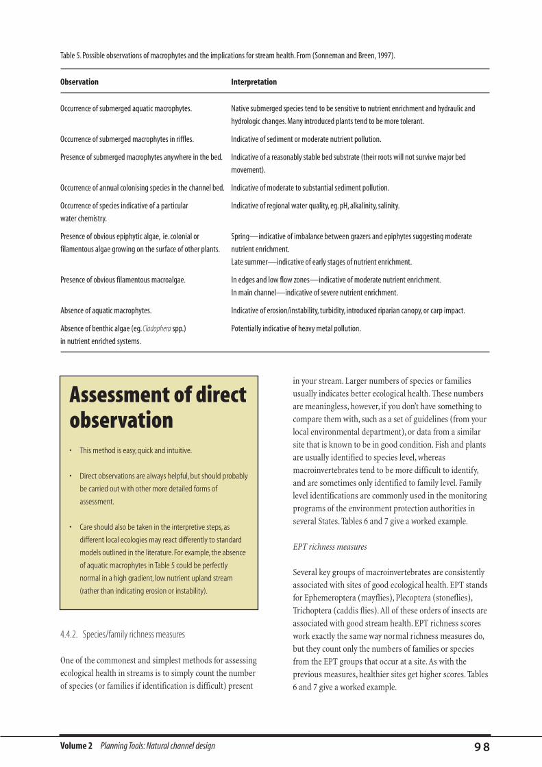
in your stream. Larger numbers of species or families
usually indicates better ecological health. These numbers
are meaningless, however, if you don’t have something to
compare them with, such as a set of guidelines (from your
local environmental department), or data from a similar
site that is known to be in good condition. Fish and plants
are usually identified to species level, whereas
macroinvertebrates tend to be more difficult to identify,
and are sometimes only identified to family level. Family
level identifications are commonly used in the monitoring
programs of the environment protection authorities in
several States. Tables 6 and 7 give a worked example.
EPT richness measures
Several key groups of macroinvertebrates are consistently
associated with sites of good ecological health. EPT stands
for Ephemeroptera (mayflies), Plecoptera (stoneflies),
Trichoptera (caddis flies). All of these orders of insects are
associated with good stream health. EPT richness scores
work exactly the same way normal richness measures do,
but they count only the numbers of families or species
from the EPT groups that occur at a site. As with the
previous measures, healthier sites get higher scores. Tables
6 and 7 give a worked example.
4.4.2. Species/family richness measures
One of the commonest and simplest methods for assessing
ecological health in streams is to simply count the number
of species (or families if identification is difficult) present
Volume 2 Planning Tools: Natural channel design 9 8
Table 5. Possible observations of macrophytes and the implications for stream health. From (Sonneman and Breen, 1997).
Observation Interpretation
Occurrence of submerged aquatic macrophytes. Native submerged species tend to be sensitive to nutrient enrichment and hydraulic and
hydrologic changes. Many introduced plants tend to be more tolerant.
Occurrence of submerged macrophytes in riffles. Indicative of sediment or moderate nutrient pollution.
Presence of submerged macrophytes anywhere in the bed. Indicative of a reasonably stable bed substrate (their roots will not survive major bed
movement).
Occurrence of annual colonising species in the channel bed. Indicative of moderate to substantial sediment pollution.
Occurrence of species indicative of a particular Indicative of regional water quality, eg. pH, alkalinity, salinity.
water chemistry.
Presence of obvious epiphytic algae, ie. colonial or Spring—indicative of imbalance between grazers and epiphytes suggesting moderate
filamentous algae growing on the surface of other plants. nutrient enrichment.
Late summer—indicative of early stages of nutrient enrichment.
Presence of obvious filamentous macroalgae. In edges and low flow zones—indicative of moderate nutrient enrichment.
In main channel—indicative of severe nutrient enrichment.
Absence of aquatic macrophytes. Indicative of erosion/instability, turbidity, introduced riparian canopy, or carp impact.
Absence of benthic algae (eg. Cladophera spp.) Potentially indicative of heavy metal pollution.
in nutrient enriched systems.
Assessment of directobservation• This method is easy, quick and intuitive.
• Direct observations are always helpful, but should probably
be carried out with other more detailed forms of
assessment.
• Care should also be taken in the interpretive steps, as
different local ecologies may react differently to standard
models outlined in the literature. For example, the absence
of aquatic macrophytes in Table 5 could be perfectly
normal in a high gradient, low nutrient upland stream
(rather than indicating erosion or instability).

Volume 2 Planning Tools: Natural channel design 9 9
4.4.3. Limitations of richness measures
The methods of assessment above assume that diversity is
the single most important ecological characteristic, and
that a stream with five species of fish in it is better than
one with a single species. This form of assessment can
sometimes prove inaccurate. If the five fish in one stream
are rainbow trout, redfin perch, and three species of carp,
while the solitary fish species in another stream is native
blackfish, then using diversity as a measure of ecological
health is deceptive. Some geographic regions are also
naturally less diverse (for example, low nutrient sand bed
streams in the Otways (Victoria)). Increasing the diversity
in one of these streams could possibly be a negative thing,
as it would suggest that the original nutrient levels had
been increased, and the new ecological system would be
less ecologically healthy even though it was more diverse.
This sort of mistake can be avoided in macroinvertebrate
studies by using a combination of richness measures and
the SIGNAL index (discussed below).
4.4.4. SIGNAL Index
The SIGNAL index (Stream Invertebrate Grade Number –
Average Level) (Chessman, 1995; Chessman et al., 1997)
sidesteps diversity, and assesses a site based on the types
of macroinvertebrates found there. In the SIGNAL system,
animals are given scores based upon whether they
commonly occur at healthy or unhealthy sites. Animals
that prefer healthy sites (such as stoneflies) have scores
closer to ten, animals like worms which can tolerate severe
pollution score closer to zero. SIGNAL indices are
calculated for individual sites by adding the scores for all
the families of animal found at a site, and dividing by the
number of families.
SIGNAL indices vary between 0 and 10, higher scores are
awarded to sites with better ecological health. Tables 6 and
7 give a worked example. SIGNAL index systems are
available for New South Wales (Chessman et al., 1997) and
Victoria (Tiller and Metzeling, 1998), but the New South
Wales system includes a methodology for tailoring the
scores to your part of Australia. Indices like these are
constantly being improved by environmental agencies, so
it is probably worth contacting your local EPA or
equivalent to see if they have been altered for the streams
and sites you want to work on.
SIGNAL indices can also be weighted by the numbers of
each type of animal occurring. A common reaction of
macroinvertebrates to mild organic pollution is an
increase in the numbers of tolerant animals such as fly
larvae and worms. These have lower SIGNAL scores which
will decrease the weighted SIGNAL index calculated at a
site. This reaction can happen before the EPT animals start
to die, so the weighted SIGNAL index is more sensitive to
mild pollution. Counting all of the individual animals in a
sample can increase the effort involved. Tables 6 and 7 give
a worked example.
Assessment ofrichness measures• This method is fairly quick, intuitive, but still requires expert
supervision.
• Biological samples have to be taken using standard
methods (Tiller and Metzeling, 1998).
• These methods require a minimum of family level
identification.
• These methods are good for comparing a number of
sites/streams, or for comparing with State environmental
guidelines.
Assessment ofSIGNAL scores• This method is fairly quick.These scores can be generated
from the same samples as the previous richness measures,
provided a relevant set of SIGNAL scores is available for
your area.
• Biological samples have to be taken using standard
methods (Tiller and Metzeling, 1998).
• Requires a minimum of family level identification (same
effort required as for richness measures).
• SIGNAL scores were developed originally to assess impacts
from organic pollutants (such as treated sewage effluent),
and are therefore best used to assess water quality.
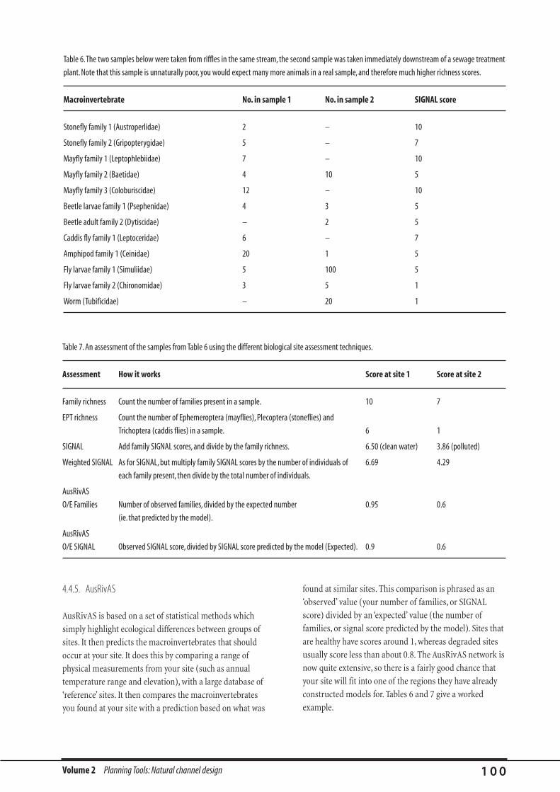
Volume 2 Planning Tools: Natural channel design 1 0 0
4.4.5. AusRivAS
AusRivAS is based on a set of statistical methods which
simply highlight ecological differences between groups of
sites. It then predicts the macroinvertebrates that should
occur at your site. It does this by comparing a range of
physical measurements from your site (such as annual
temperature range and elevation), with a large database of
‘reference’ sites. It then compares the macroinvertebrates
you found at your site with a prediction based on what was
Table 6.The two samples below were taken from riffles in the same stream, the second sample was taken immediately downstream of a sewage treatment
plant. Note that this sample is unnaturally poor, you would expect many more animals in a real sample, and therefore much higher richness scores.
Macroinvertebrate No. in sample 1 No. in sample 2 SIGNAL score
Stonefly family 1 (Austroperlidae) 2 – 10
Stonefly family 2 (Gripopterygidae) 5 – 7
Mayfly family 1 (Leptophlebiidae) 7 – 10
Mayfly family 2 (Baetidae) 4 10 5
Mayfly family 3 (Coloburiscidae) 12 – 10
Beetle larvae family 1 (Psephenidae) 4 3 5
Beetle adult family 2 (Dytiscidae) – 2 5
Caddis fly family 1 (Leptoceridae) 6 – 7
Amphipod family 1 (Ceinidae) 20 1 5
Fly larvae family 1 (Simuliidae) 5 100 5
Fly larvae family 2 (Chironomidae) 3 5 1
Worm (Tubificidae) – 20 1
found at similar sites. This comparison is phrased as an
‘observed’ value (your number of families, or SIGNAL
score) divided by an ‘expected’ value (the number of
families, or signal score predicted by the model). Sites that
are healthy have scores around 1, whereas degraded sites
usually score less than about 0.8. The AusRivAS network is
now quite extensive, so there is a fairly good chance that
your site will fit into one of the regions they have already
constructed models for. Tables 6 and 7 give a worked
example.
Table 7. An assessment of the samples from Table 6 using the different biological site assessment techniques.
Assessment How it works Score at site 1 Score at site 2
Family richness Count the number of families present in a sample. 10 7
EPT richness Count the number of Ephemeroptera (mayflies), Plecoptera (stoneflies) and
Trichoptera (caddis flies) in a sample. 6 1
SIGNAL Add family SIGNAL scores, and divide by the family richness. 6.50 (clean water) 3.86 (polluted)
Weighted SIGNAL As for SIGNAL, but multiply family SIGNAL scores by the number of individuals of 6.69 4.29
each family present, then divide by the total number of individuals.
AusRivAS
O/E Families Number of observed families, divided by the expected number 0.95 0.6
(ie. that predicted by the model).
AusRivAS
O/E SIGNAL Observed SIGNAL score, divided by SIGNAL score predicted by the model (Expected). 0.9 0.6

• Water quality
Changes in water quality can influence the condition of
downstream reaches.
• Bed degradation
Bed degradation usually moves upstream, so consider how
downstream headcuts would effect the reach if allowed to
continue upstream.
• Recolonisation sources
Rehabilitation of streams requires the presence of
adequate populations for recolonisation, such as seeds
from upstream forests for revegetation, or fish populations
from upstream or downstream reaches.
Now that you have described the condition of your stream
reach, it is time to see how the reaches interact with each
other.
Streams are usually continuous longitudinal systems, so
the arbitrarily defined reaches are not isolated—they
interact. Identifying these interactions between reaches is
one of the key tasks in effective stream and catchment
management. The sorts of issues you need to consider in
terms of the interconnectedness of the stream are:
• Sediment
What are the sediment sources and depositional zones and
how are they affecting downstream reaches? For example,
a reach of willows may be trapping sediment from
upstream reaches, in which case you would have to
consider the downstream ramifications of removing the
willows and releasing the sediment. The Brierley ‘River
Styles’ method provides an approach to predicting change
in the stream system (see Channel evolution approaches to
channel design).
Volume 2 Planning Tools: Natural channel design 1 0 1
5. Determining the interactions between reaches
At this point you should have a look at Common stream problems
(this volume).You may recognise your stream problem type
there, and this may help in the following assessments.
Assessment of AusRivASThis method is complicated and requires professional assistance. More information available at the web site
http://ausrivas.canberra.edu.au/ausrivas/
• Biological samples have to be taken using standard methods (Tiller and Metzeling, 1998).
• If the analysis is done by an anvironmental agency, the results can be distilled into an easily interpreted report.
• AusRivAS requires a suite of environmental and water quality data to be taken at the same time as the biological samples, and for this reason
requires a serious commitment. Different regions require different types of data, so it is important to check that you are looking for the right
data before you start.

Volume 2 Planning Tools: Natural channel design 1 0 2
An important task in stream rehabilitation is to correctly
identify which problem needs to be fixed in order to improve
the streams natural assets. There is no point developing
elaborate rehabilitation plans to treat the wrong problem, or
to fix a symptom and not the cause. Some hypothetical
examples of incorrect identification of causes are:
• Stream managers remove trees from the stream banks
in the belief that they cause bank slumping. In reality
the trees are falling in because the bed is deepening,
and the banks are becoming unstable.
• Managers build in-stream structures to restore habitat,
when it turns out that the declining fish population
were caused by predation by trout.
• Anglers blame flow regulation from a dam for the poor
fish numbers, only to discover that they have been
fishing in pools that have become saline.
Problem definition is a matter of perspective and depends
on the values attached to the river. A problem is usually
expressed as a symptom, such as "fish numbers have
declined" or "the river is eroding". These descriptions of a
problem do not, in themselves, explain the problem. An
explanation is needed for the river manager to be
empowered to effectively address the problem. Some
problems are not as simply explained as they may initially
seem. The difficulty of isolating changes due to a host of
human disturbances superimposed over natural
variability and changes, means that it is advisable to seek
specialised scientific assistance to investigate the cause of
river problems.
Environmental problems in streams are usually defined in
terms of their impact on a specific organism (eg. fish,
platypus, macroinvertebrates), or in terms of generic
deficiencies in stream health: poor riparian vegetation,
poor water quality, erosion and deposition.
If your interest is in organisms in a stream, then
population declines can relate to habitat, breeding, water
quality, food supply, hydrology and predation. The changes
can be related to the magnitude, duration and frequency of
impacts. For example:
• Turbidity levels can usually rise dramatically for short
periods with little impact on organisms, but long
periods of slightly higher turbidity could harm some
species.
• The demise of one organism could be a secondary
effect of the disappearance of another (eg.
macroinvertebrates disappear because they are
smothered by sediment, leading to a loss of a fish
species that relied on them for food).
Table 8 shows some factors that could be influencing the
organisms in your stream. In reality there are probably
many of these factors influencing the abundance and
diversity of organisms in the reach. However, it may be that
one or two of these factors is of overriding importance—a
‘fatal’ or limiting problem. Until these are corrected, there
is little point tackling the rest of your problems.
6.1. Biological limits approach
6. Determining the key problems in the reach
This section provides more information for Step 4 What are the
stream’s main assets and problems? and Step 5 Setting priorities: which
reaches and problems should you work on first? in the Stream
rehabilitation procedure (Volume 1).
It is not the purpose of this manual to tell you how to diagnose
all possible problems in your streams (although Common
stream problems (this volume) provides some detailed
information on the more common problems) and, more
importantly, we cannot tell you why a particular problem
exists (eg. why a particular fish has disappeared, or why this
bank is eroding).This is very often a specialised, site-specific
task. But what we can do is describe some approaches that
you can use to diagnose the cause, and the range of possible
problems that you could face.
The concept of biological limits is also discussed in An
introduction to stream ecosystems, in Stream rehabilitation
concepts, in Volume 1.

Volume 2 Planning Tools: Natural channel design 1 0 3
Table 8. Some examples of problems that directly influence stream organisms by impacting on their major requirements, and some stream processes or
human impacts that could cause those problems.
Major requirement Problem Possible process or human impact that could cause the problem
Habitat Reduced cover, ie. limited large woody debris (LWD), Channelisation—removal of LWD, and vegetation.
undercutting,overhanging vegetation or larger rocks.
Limited velocity variability. Homogenisation of streams by erosion, channelisation, sediment slugs.
Low depth variability. Pools filled with sediment (homogenisation), removal of LWD and
other obstructions.
Uniform substrate: fine material. Unstable beds, eroded clay beds, sand slugs, fine sediment filling spaces
between gravels.
Uniform substrate: coarse material. Increase in regulated discharge below a dam leads to more regular
movement of bed-material, stock trampling, sand and gravel extraction.
Reduced shade. Vegetation removal, reduced cover; decreased depth with bed aggradation.
Breeding Reduced flooding limits floodplain access for breeding. Dams reduce flooding.
Low egg survival. Sedimentation on rocks, increased velocities.
Limited nursery areas for young fish. Channelisation reduces habitat diversity, hydraulic diversity.
Water quality Turbidity levels too high. Increased catchment and channel erosion.
Dissolved oxygen levels too low. Levels decreased by decomposition of increased organic matter, increased
temperature in still water.
Temperature too low or high. Reduced temperature from low-level dam releases, elevated temperature
with reduced shade or from wide, shallow streams.
Nutrient levels too high. Elevated by agricultural run-off, sewage treatment, or channel erosion.
High or low pH, high levels of heavy Point source enrichment issues such as mining, industrial processes,
metals and pesticides. agriculture.
Food and nutrient Low food input from vegetation. Inadequate riparian vegetation to provide food (leaf litter, flowers,
supply fruit, insects).
Lack of large woody debris. Desnagging of streams removes an essential food source in lowland
streams.
Low food distribution downstream. Dams trap organic material moving downstream.
Low food input from floodplains. Reduced flooding decreases organic debris and carbon from floodplains.
Not enough food due to competition. Exotic fish and other creatures can out-compete native species for food.
Hydrology Shorter flood duration. Regulation of stream for drinking water and irrigation.
Stream communities changed from riverine to lake. Dams and weirs change the character of the stream.
Altered seasonality of flows. Altered seasonality from dam storage and releases affects breeding.
Lower flood frequency. Reduced flooding affects breeding and food sources.
Increased rate of change. Rapid rises and falls of stage leave organisms stranded.
Fish passage Barriers to fish passage. Low weirs, culverts, fords, shallow wide expanses of water,
high-velocity water.
Predation balance Predation. Exotic species can eat native species.
The ‘biological limits approach’ sets out to identify the
critical factors that control the population of particular
target organisms. This approach can be called the ‘limits’
approach, because it is targeting the main limiting factor
for a particular faunal group. The rehabilitation program is
then aimed at providing these factors in the most
appropriate way; for example, by altering flow regime,
improving water quality, or by building in-stream habitat
structures (Swales, 1989; Beschta et al., 1994). This
approach requires that the habitat requirements for the
target fauna be known. Unfortunately, it is seldom the case
that these are known in detail.

Volume 2 Planning Tools: Natural channel design 1 0 4
If you are interested in identifying habitat deficiencies for
specific organisms, then descriptions of habitat
requirements exist for some species. By comparing your
reach with the description in Table 9, or in the detailed
descriptions of native fish habitat in Koehn and O’Connor
(1990), you can attempt to tailor your reach to the
requirements. Such habitat matching has reached a very
detailed stage for salmonids in the northern hemisphere,
where they can specify exactly the particle-size
distribution required for spawning, or the radius of
curvature of bends preferred by trout.
6.1.1. How do you know what the limiting variable is?
One crude, but useful, way to identify some limiting
variables is to look for places that have the characteristics
that you want to achieve, and see if they have the
environmental values that you are looking for. For
example, is in-stream habitat the limiting physical variable
for macroinvertebrate population diversity in your reach?
Try inspecting any portion of the stream that already
provides elements of the physical habitat that you are
interested in restoring. Do these habitats have satisfactory
populations of the organisms that you are interested in
fostering? If not, then do not expect to be too successful
with your own habitat enhancement. It would be wise to
look for other limiting variables.
Other examples of the same approach would be:
• The effects of flow regulation often decline downstream
in a stream system. Do you find a corresponding
downstream improvement in the target organism? If
not, it may suggest that there are more complex
problems that may not be related to flow regulation.
• For riparian vegetation, ask yourself "why is there
riparian vegetation here and not there?" Why hasn’t it
regenerated? Could it be because there is no seed
source, because the erosion rate on the bend is too great
and the regenerating vegetation is being washed away,
or because stock grazing is preventing revegetation?
6.1.2 . Concluding comments on identifying limiting variables
It is important to emphasise that, even with the methods
described here, you may not be able to identify the limiting
environmental variable in your reach, or explain why a
trend exists. For example, despite detailed sampling and
monitoring, scientists are still unable to explain why the
Broken River in northern Victoria has a much richer fish
fauna than its neighbouring stream, the Campaspe River.
Is this a trend (ie. a decline in once higher diversity in the
Campaspe), or could it be something to do with the larger
dam on the Campaspe River?
Table 9. Criteria for assessment of fish habitat values for the Numerella River (information is based on the requirements of two native species, trout cod and
Maquarie perch and of the introduced species, brown trout). From The Numeralla: River of Change, by Barry Starr (1995).
Feature Undesirable Desirable
Gradient Regular and even so that water depth remains constant. Regular grade changes, sequence of pools and riffles.
Cross-section Regular and even. Variable, a mixture of deep holes (>1.5 m), shallow areas, wide and
shallow riffles, narrow and deep riffles.
Bed material Uniform composition—whether rock, shingle, pebble, Mixture of large boulders and cobbles, smaller shingle, pebbles,
mud or sand. sand and mud.
Aquatic flora Few or no aquatic plants. Abundance of only 1 or 2 species Range of species (reeds, pond weeds, milfoils etc.) distributed
or aquatic plants. Abundance of filamentous algae. throughout the stream. Little if any filamentous algae.
Riparian vegetation Little or no riparian vegetation. Abundance of More or less continuous and wide fringe of a range of native species
non-native trees or shrubs (eg. willows). (trees, shrubs, herbs, grasses). Provides shade, input of food and organic
matter, enhances bank stability.
Instream cover Few if any logs, large boulders, steep banks etc. which Logs, large boulders, steep banks etc. are common to abundant
provide refuge from the flow and predators. throughout the stream.
Water quality Low levels of dissolved oxygen (ie. <5 mg/L). Moderate to high levels of dissolved oxygen (6–10 mg/L).
Low pH levels (ie. <6.5). Neutral to slightly alkaline pH levels (ie. 6.5–9.0).
Temperature High water temperature (ie. >23°C). Low to moderate water temperature.

Volume 2 Planning Tools: Natural channel design 1 0 5
A hypothetical example of the importance oftargeting the limiting problemThe lower Problematic River is in fair to poor condition. It is fairly typical of the streams in the region.The banks are mostly lined with willows, but
there are pockets of intact native riparian vegetation.There is some local bank erosion, but generally the river morphology is relatively
undisturbed (gravel bed, pool–riffle sequence).There is good potential to rehabilitate the stream by improving riparian vegetation, and
controlling stock access to the stream.There are also two large dams on the river. If the stream manager’s goal is to return the stream to
something like its pre-European settlement state, with a full complement of native fish, what should be done?
Fortunately we know a lot about the Problematic River, because extensive baseline studies of the fish fauna were done before the upper dam
was built. At the time the fish biologists urged the dam designers to build a multi-level water off-take because the water released from the dam
would be too cold for native fish to survive.The multi-level off-take was not built. Later surveys showed that the healthy populations of native
fish were no longer present in the river, and had been replaced by brown trout.The reason, as predicted, was the low temperature of water
released from the dam.
Stream managers on the Problematic River can draw two conclusions. First, fish numbers were healthy before the dam was built, suggesting that
in-stream habitat was not fatally degraded for fish, although it could probably be improved.The in-stream habitat has not changed much since
the dam was built. Second, the limiting variable for fish (at least) along this stream is water temperature, and this is the problem that must be
targeted first.
Thus, if the return of native fish and other creatures to the Problematic River is the manager’s primary goal, then they should put their resources
into increasing the temperature of water released from the dam, so that it is closer to the natural temperature range.The natural range is known
in this case, but otherwise it could have been estimated from the range of temperatures in a template reach.
The stream manager would then ask three more questions:
• What temperature ranges would be acceptable if I could not achieve the original temperature range? (Having this compromise position is
essential for negotiations.) In this case, temperatures within the known range of tolerance of the native fish would be acceptable.
• If acceptable temperatures are achieved, can the fish return? First check if any fish at all survive in the river. Are there enough for a breeding
population? The Problematic River runs into another large dam downstream.This could prevent migration of fish into the Problematic River.
Fish may have to be artificially restocked.
• If the fish were artificially restocked would their populations be sustainable? Since they existed before the upper reservoir was built, the
population probably would be sustainable.

Volume 2 Planning Tools: Natural channel design 1 0 6
Assessment of the limits approachBy Michael Stewardson*
It is difficult to know which variable is the most important in limiting the success of an organism.This habitat-based approach has been widely
applied in the United States, but in some cases it has been shown to be unsuccessful. For example, a review of over 1,200 stream restoration
projects in Oregon revealed that early stream restoration efforts concentrated largely on creating pools for summer fish habitat. Recent research
has shown that for many Oregon streams, pool habitat is not necessarily the factor limiting fish productivity, and the focus for restoration of
streams in Oregon is now the provision of cover as refuge for young fish during high winter flows (Andrus, 1991). Similarly, in south-eastern
Australia, the provision of in-stream cover is emerging as a critical factor in determining fish populations (Koehn, 1987).
The habitat enhancement approach requires that habitat requirements for the species at different life-stages have been established (Hey, 1992),
and that factors currently limiting productivity are correctly identified (Hicks and Reeves, 1994). It is also possible that efforts to enhance the
habitat of a limited faunal group may ignore, or have a detrimental effect on, other members of the aquatic community (National Research
Council, 1992). Even when expertly done, modifications intended to maximise habitat may result in symptomatic treatment of perceived defects
from the perspective of one or a few fish species. Current stream restoration practices are rarely based on sufficient knowledge of the physical-
habitat requirements of the biota (Borchadt, 1993).
A key characteristic of productive streams is habitat diversity (Gorman and Karr, 1978;Wesche, 1985). Hicks and Reeves (1994) argue that the
impact of restoration efforts must be considered in the context of the fish community and not just a single species or age-class. For this reason,
many projects are now attempting to create a variety of habitat conditions that will potentially benefit all fish species and ages.The object of
these restoration projects is frequently termed ‘habitat diversity’, although this term is rarely defined.
* Department of Civil and Environmental Engineering, University of Melbourne, Parkville,Victoria 3052. Email: [email protected]

European settlement. It is important to note that it was the
stream ‘processes’ that were undisturbed at that time. By
processes, we mean the things that drive the system and give
it its character, such as the catchment hydrology, the
sediment transport system, the ecological interactions, and
the in-stream habitat hydraulics.Attempting to restore the
detailed physical characteristics of the stream (such as
channel width, meander shape or pool–riffle sequence) as it
existed perhaps 150 years ago could fail to produce the
expected ecological recovery if the driving processes have
substantially altered since that time. In this case it is
necessary to adjust expectations by scaling the potential
Volume 2 Planning Tools: Natural channel design 1 0 7
With contributions from Dr Chris Gippel *
DESIGNING A MORE NATURAL STREAM
This section deals with streams that have undergone some
substantial modification to their basic form, or
morphology, so that they are regarded as degraded (or
ecologically inferior) compared to with their pre-
disturbance condition. Before undertaking any kind of
stream works that aim to ‘naturalise’ a stream, it is important
to set some realistic and meaningful objectives. The term
‘natural’ is so subjective, that, on its own, it is inadequate as
an objective.A possible starting point is to determine the
ecological potential of the stream—what it would be like if
there was no significant human disturbance? It can be
assumed that the stream was in this condition before
1 . Setting realistic objectives
This part of the manual links to Step 9 of the Stream rehabilitation procedure (Volume 1) How will you design your project to achieve your
objectives ? It also describes approaches for developing a template of the desirable condition of your stream (Task 2, Step 3, How has your stream
changed since European settlement ?
If you have gone through the procedure you may have decided that you want to directly intervene in a stream to make it more ‘natural’.
This section of the manual describes a procedure that you can follow to design a more natural stream and provides information on:
• the limitations of recreating ‘natural’ streams;
• applications and limitations of the available channel- design procedures; and
• what to measure when developing a template of another stream.
WARNING!Is it time for you to be exploring this section yet? It is very tempting to explore the possibility of rebuilding your damaged stream.This is a very
common activity around the world, and there are good design guides available for doing it. However, the prioritisation procedure (Step 5)
emphasises that the first task of stream rehabilitation is to protect the natural assets that remain in streams.We should only be considering
improving stream reaches when we have protected the assets that already exist. So we should only really be contemplating rebuilding a more
‘natural’ stream if we are confident that we have already protected the remaining natural assets.
* Fluvial Systems, PO Box 4117, Melb.uni.Retail, Parkville,Victoria 3052. Email 1: [email protected] Email 2: [email protected]
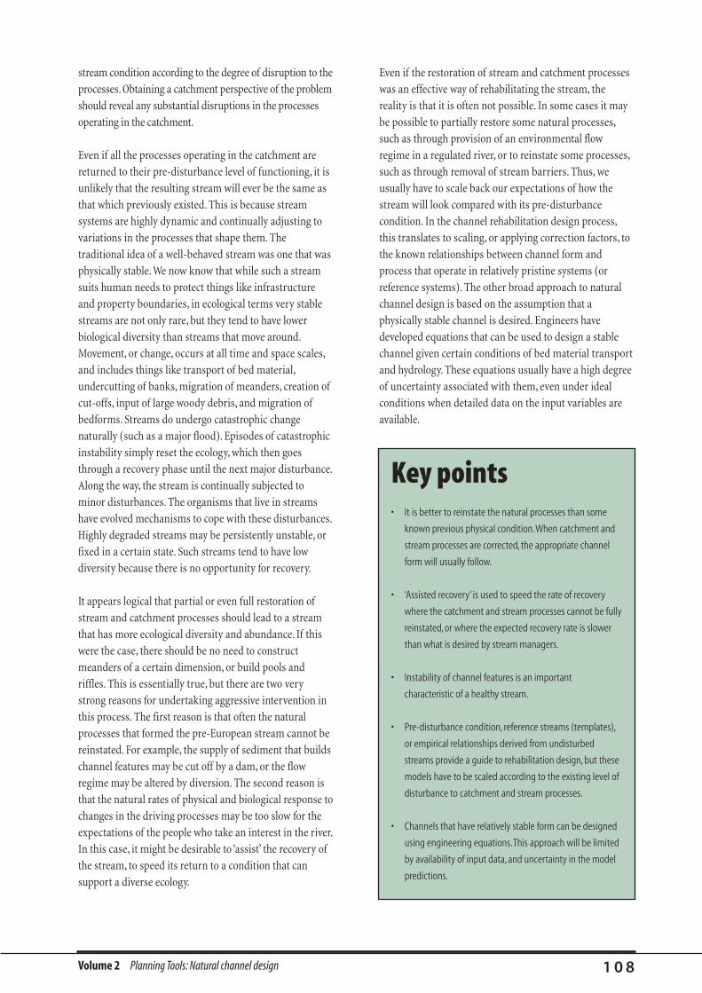
Volume 2 Planning Tools: Natural channel design 1 0 8
stream condition according to the degree of disruption to the
processes. Obtaining a catchment perspective of the problem
should reveal any substantial disruptions in the processes
operating in the catchment.
Even if all the processes operating in the catchment are
returned to their pre-disturbance level of functioning, it is
unlikely that the resulting stream will ever be the same as
that which previously existed. This is because stream
systems are highly dynamic and continually adjusting to
variations in the processes that shape them. The
traditional idea of a well-behaved stream was one that was
physically stable. We now know that while such a stream
suits human needs to protect things like infrastructure
and property boundaries, in ecological terms very stable
streams are not only rare, but they tend to have lower
biological diversity than streams that move around.
Movement, or change, occurs at all time and space scales,
and includes things like transport of bed material,
undercutting of banks, migration of meanders, creation of
cut-offs, input of large woody debris, and migration of
bedforms. Streams do undergo catastrophic change
naturally (such as a major flood). Episodes of catastrophic
instability simply reset the ecology, which then goes
through a recovery phase until the next major disturbance.
Along the way, the stream is continually subjected to
minor disturbances. The organisms that live in streams
have evolved mechanisms to cope with these disturbances.
Highly degraded streams may be persistently unstable, or
fixed in a certain state. Such streams tend to have low
diversity because there is no opportunity for recovery.
It appears logical that partial or even full restoration of
stream and catchment processes should lead to a stream
that has more ecological diversity and abundance. If this
were the case, there should be no need to construct
meanders of a certain dimension, or build pools and
riffles. This is essentially true, but there are two very
strong reasons for undertaking aggressive intervention in
this process. The first reason is that often the natural
processes that formed the pre-European stream cannot be
reinstated. For example, the supply of sediment that builds
channel features may be cut off by a dam, or the flow
regime may be altered by diversion. The second reason is
that the natural rates of physical and biological response to
changes in the driving processes may be too slow for the
expectations of the people who take an interest in the river.
In this case, it might be desirable to ‘assist’ the recovery of
the stream, to speed its return to a condition that can
support a diverse ecology.
Even if the restoration of stream and catchment processes
was an effective way of rehabilitating the stream, the
reality is that it is often not possible. In some cases it may
be possible to partially restore some natural processes,
such as through provision of an environmental flow
regime in a regulated river, or to reinstate some processes,
such as through removal of stream barriers. Thus, we
usually have to scale back our expectations of how the
stream will look compared with its pre-disturbance
condition. In the channel rehabilitation design process,
this translates to scaling, or applying correction factors, to
the known relationships between channel form and
process that operate in relatively pristine systems (or
reference systems). The other broad approach to natural
channel design is based on the assumption that a
physically stable channel is desired. Engineers have
developed equations that can be used to design a stable
channel given certain conditions of bed material transport
and hydrology. These equations usually have a high degree
of uncertainty associated with them, even under ideal
conditions when detailed data on the input variables are
available.
Key points• It is better to reinstate the natural processes than some
known previous physical condition.When catchment and
stream processes are corrected, the appropriate channel
form will usually follow.
• ‘Assisted recovery’ is used to speed the rate of recovery
where the catchment and stream processes cannot be fully
reinstated, or where the expected recovery rate is slower
than what is desired by stream managers.
• Instability of channel features is an important
characteristic of a healthy stream.
• Pre-disturbance condition, reference streams (templates),
or empirical relationships derived from undisturbed
streams provide a guide to rehabilitation design, but these
models have to be scaled according to the existing level of
disturbance to catchment and stream processes.
• Channels that have relatively stable form can be designed
using engineering equations.This approach will be limited
by availability of input data, and uncertainty in the model
predictions.
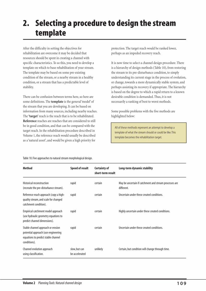
After the difficulty in setting the objectives for
rehabilitation are overcome it may be decided that
resources should be spent in creating a channel with
specific characteristics. To so this, you need to develop a
template on which to base rehabilitation of your stream.
The template may be based on some pre-existing
condition of the stream, or a nearby stream in a healthy
condition, or a stream that has a predictable level of
stability.
There can be confusion between terms here, so here are
some definitions. The template is the general ‘model’ of
the stream that you are developing. It can be based on
information from many sources, including nearby reaches.
The ‘target’ reach is the reach that is to be rehabilitated.
Reference reaches are reaches that are considered to still
be in good condition, and that can be compared with the
target reach. In the rehabilitation procedure described in
Volume 1, the reference reach would usually be described
as a ‘natural asset’, and would be given a high priority for
Volume 2 Planning Tools: Natural channel design 1 0 9
protection. The target reach would be ranked lower,
perhaps as an impeded recovery reach.
It is now time to select a channel design procedure. There
is a hierarchy of design methods (Table 10), from restoring
the stream to its pre-disturbance condition, to simply
understanding its current stage in the process of evolution,
or change, towards a more dynamically stable system, and
perhaps assisting its recovery if appropriate. The hierarchy
is based on the degree to which a rapid return to a known
desirable condition is demanded. Thus, it is not
necessarily a ranking of best to worst methods.
Some possible problems with the five methods are
highlighted below:
2. Selecting a procedure to design the stream template
Table 10. Five approaches to natural stream morphological design.
Method Speed of result Certainty of Long-term dynamic stability
short-term result
Historical reconstruction rapid certain May be uncertain if catchment and stream processes are
(recreate the pre-disturbance stream). different.
Reference reach approach (copy a high- rapid certain Uncertain under these created conditions.
quality stream, and scale for changed
catchment condition).
Empirical catchment model approach rapid certain Highly uncertain under these created conditions.
(use hydraulic geometry equations to
predict channel dimensions).
Stable channel approach or erosion rapid certain Uncertain under these created conditions.
potential approach (use engineering
equations to predict stable channel
conditions).
Channel evolution approach slow, but can unlikely Certain, but condition will change through time.
using classification. be accelerated
All of these methods represent an attempt to develop a
template of what the stream should or could be like.This
template becomes the rehabilitation target.

Volume 2 Planning Tools: Natural channel design 1 1 0
• Historical reconstruction: reconstruct the original
condition of the stream from historical information
(eg. use the pre-disturbance stream form as a template
for rehabilitation).
• Reference reach approach: copy the characteristics of
a remnant of a good quality stream (eg. use a good-
quality upstream, downstream or nearby stream reach
as a template for rehabilitation).
• Empirical catchment model approach: apply generic,
empirical relationships, based on hydraulic geometry, or
regime relationships to predict the ‘equilibrium’ form of
the stream (eg. use width/discharge relationships,
planform/width relationships to predict an equilibrium
channel form that you can use as a basis for stable
channel design).
• Stable channel or erosion potential approaches:
include the hydraulic–geomorphic approach and tractive
stress or maximum allowable velocity approaches which
allows a stable bed slope to be predicted such that there
is no net degradation of the reach.
• Channel evolution approach using classification:
use conceptual models of the morphological stages
through which a stream evolves after major
disturbance. By classifying the stage of evolution its
relative stability can be assessed, and its recovery path
predicted. The evolutionary process can be speeded by
assisted recovery techniques that might involve
revegetation or in-stream structures.
Problems:Catchment and floodplain conditions may have
changed so much that the original form is no longer appropriate.
Problems:There may be no reach available, or the only reach is
too far away to be strictly comparable.
Problems:Bedload equations used in the hydraulic–geomorphic
approach are notoriously inaccurate, so even though this
appears to be a ‘scientific’numerical solution to predicting a
stable bed, we need to be aware of its limitations.
The tractive stress approach assumes cross-section average
values, but we know that flow velocities are concentrated in
certain parts of the channel, so the tractive stress is not evenly
distributed across the channel cross- section.We do not
discuss this approach further.
Problems: Empirical relationships are notoriously unreliable
when applied to different rivers, and must assume that
streams used in data sets were in equilibrium. Uncertainty
about application to Australian streams.
Where to find moreinformation on thefive approaches todesigning yourstream template• Historical reconstruction is discussed below in Using historical
reconstruction to develop a template.
• The reference reach approach is discussed below in Using a
reference reach to develop a template.
• The empirical catchment model approach is discussed in
the next section Empirical approaches to designing a
naturally stable channel.
• The stable channel or erosion potential approaches are not
discussed further in this manual.
• The channel evolution approach is discussed in the
following section Channel evolution approach to
rehabilitation design.
Problems: Channel recovery may take too long to satisfy the
expectations of stream managers and the general community.
There is a level of uncertainty in the form that the channel will
take through time.
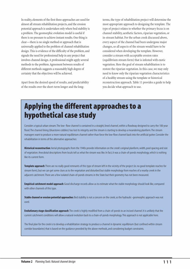
Volume 2 Planning Tools: Natural channel design 1 1 1
In reality, elements of the first three approaches are used for
almost all stream rehabilitation projects, and the erosion
potential approach is undertaken only where bed stability is
a problem. The geomorphic evolution model is useful if
there is no pressure to achieve instant results. One thing is
clear—there is no single method or approach that is
universally applied to the problem of channel rehabilitation
design. This is evidence of the difficulty of the problem, and
signals the need for professional help in any project that
involves channel design.A professional might apply several
methods to the problem.Agreement between results of
different methods suggests a reasonably high degree of
certainty that the objectives will be achieved.
Apart from the desired speed of results, and predictability
of the results over the short-term longer and the long-
terms, the type of rehabilitation project will determine the
most appropriate approach to designing the template. The
type of project relates to whether the primary focus is on
channel stability, aesthetic factors, riparian vegetation, or
in-stream habitat. For the urban creek discussed above,
every aspect of the channel had been undergone major
changes, so all aspects of the stream would have to be
considered when developing the template. However,
consider a stream with acceptable erosion rates
(equilibrium stream form) that is infested with exotic
vegetation. Here the goal of stream rehabilitation is to
restore the riparian vegetation. In this case, we may only
need to know only the riparian vegetation characteristics
of a healthy stream using the template or historical
reconstruction approach. Table 11 provides a guide to help
you decide what approach to use.
Applying the different approaches to ahypothetical case studyConsider a typical urban stream.The low- flow channel is contained in a straight, lined channel, within a floodway designed to carry the 100 year
flood.The channel lining (bluestone cobbles) has lost its integrity and the stream is starting to develop a meandering planform.The stream
managers want to produce a more natural equilibrium channel rather than force the low-flow channel back into the artificial gutter. Consider the
rehabilitation in terms of the alternative approaches:
Historical reconstruction: Aerial photographs from the 1940s provide information on the creek’s original planform, width, pool spacing and size
of vegetation. Anecdotal descriptions from locals tell us what the stream was like. In fact, it was a chain-of-ponds morphology, which is nothing
like its current form.
Template approach:There are no really good remnants of this type of stream left in the vicinity of the project (ie. no good template reaches for
stream form), but we can get some clues as to the vegetation and disturbed but stable morphology from reaches of a nearby creek in the
adjacent catchment.There are a few isolated chain-of-ponds streams in the State but their geometry has not been measured.
Empirical catchment model approach: Good discharge records allow us to estimate what the stable morphology should look like, compared
with other channels of this type.
Stable channel or erosion potential approaches: Bed stability is not a concern on the creek, so the hydraulic–geomorphic approach was not
used.
Evolutionary stage classification approach:The creek is highly modified from a chain-of-ponds to an incised channel. It is unlikely that the
current catchment conditions will allow a natural evolution back to a chain-of-ponds morphology.This approach is not applicable here.
The final plan for the creek is to develop a rehabilitation strategy to produce a channel in dynamic equilibrium (but confined within stream
corridor boundaries) that is based on the guidance provided by the above methods, and considering budget constraints.
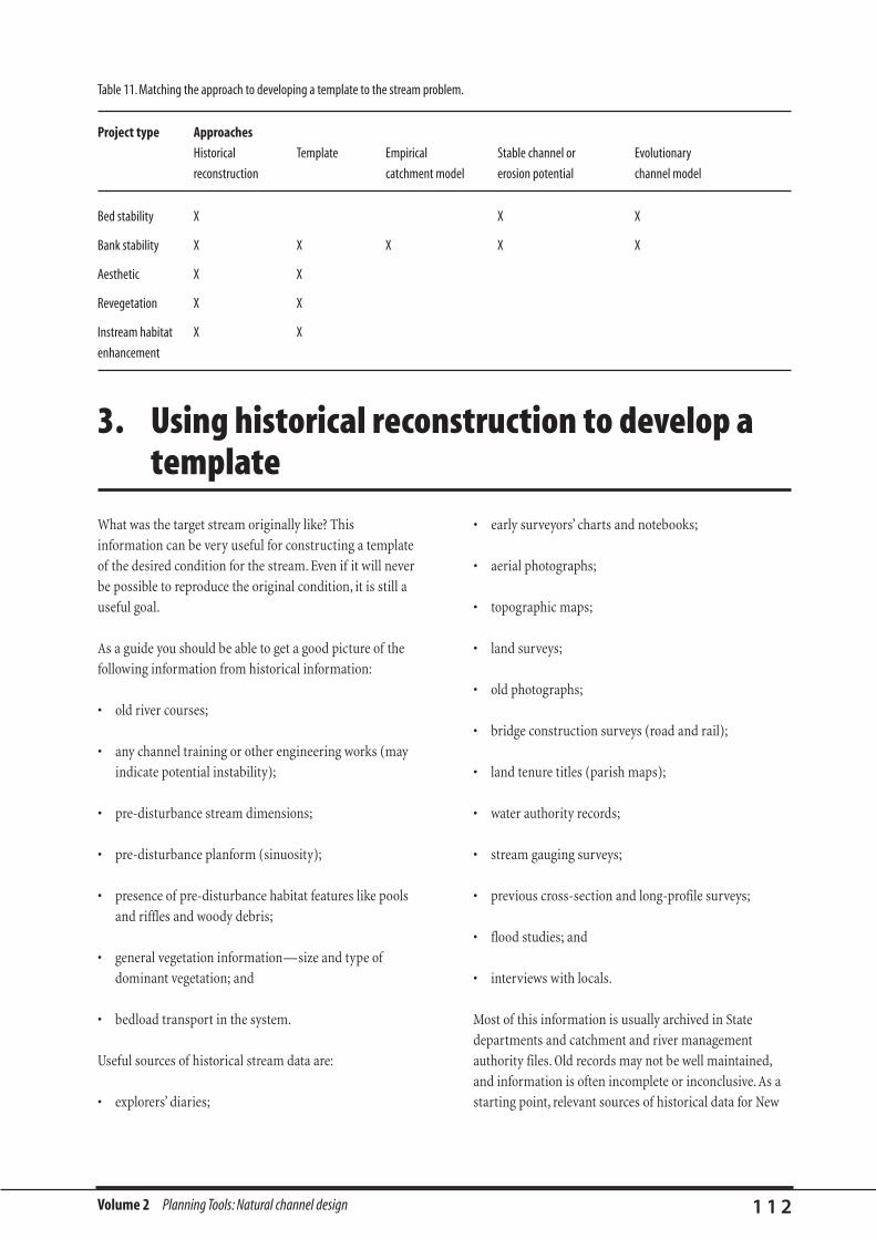
Volume 2 Planning Tools: Natural channel design 1 1 2
What was the target stream originally like? This
information can be very useful for constructing a template
of the desired condition for the stream. Even if it will never
be possible to reproduce the original condition, it is still a
useful goal.
As a guide you should be able to get a good picture of the
following information from historical information:
• old river courses;
• any channel training or other engineering works (may
indicate potential instability);
• pre-disturbance stream dimensions;
• pre-disturbance planform (sinuosity);
• presence of pre-disturbance habitat features like pools
and riffles and woody debris;
• general vegetation information—size and type of
dominant vegetation; and
• bedload transport in the system.
Useful sources of historical stream data are:
• explorers’ diaries;
• early surveyors’ charts and notebooks;
• aerial photographs;
• topographic maps;
• land surveys;
• old photographs;
• bridge construction surveys (road and rail);
• land tenure titles (parish maps);
• water authority records;
• stream gauging surveys;
• previous cross-section and long-profile surveys;
• flood studies; and
• interviews with locals.
Most of this information is usually archived in State
departments and catchment and river management
authority files. Old records may not be well maintained,
and information is often incomplete or inconclusive. As a
starting point, relevant sources of historical data for New
Table 11. Matching the approach to developing a template to the stream problem.
Project type Approaches
Historical Template Empirical Stable channel or Evolutionary
reconstruction catchment model erosion potential channel model
Bed stability X X X
Bank stability X X X X X
Aesthetic X X
Revegetation X X
Instream habitat X X
enhancement
3. Using historical reconstruction to develop a template

Volume 2 Planning Tools: Natural channel design 1 1 3
South Wales are presented in Table 12. Similar information
is available in most States. It is a matter of doing the
detective work to see what you can find out about your
stream.
At best, historical records are likely to provide a picture of
the type and location of the stream. Accurate dimensions
Table 12. Sources of historical information for New South Wales streams. Source: Brierley et al. (1996), based on Herron (1993).
Location Information held Comments
Lands Department. Portion plans. Contains vegetation information and comments on available surface water.
Occasionally have nothing at all except the types of trees used as portion markers.
Bridge surveys. Invaluable for assessing changes in channel structure, ie. widths and depths.
Surveyors field books.
Parish maps. Show portion numbers, boundaries and first property owner.
Recent air photographs. Can inspect these.
Older air photographs. Earliest date from 1940s. Problems include delays and poor indexing.
Topographic maps.
Mitchell Library, Old maps, correspondences, There is a lot of information kept here, but there is a certain amount of pot luck in
Sydney. books, journals, small finding what you are looking for. Be patient.
picture files, laser disk
storage of photographs,
some newspapers.
State Library of Books, journals, newspapers. This is the best place for looking up newspapers.
NSW, Sydney.
Archives Office of Maps field notebooks, journals.
NSW,The Rocks,
Sydney, or Kingswood.
Land Titles Office, Sydney. Portion plans. The plans are all on microfilm.
Bureau of Meteorology, Rainfall data—monthly means, Length of records for daily data generally less.
Sydney. also daily data from most stations,
temperatures, frosts, winds etc.
Department of Land Air photographs.
and Water Conservation. Historical records of stream work.
AUSLIG Air photographs.
Australian National Library Books, journals, maps, early air
of Australia, Canberra. photographs, oral histories, newspapers.
Historical societies. Newspaper clippings, letters, journals, Often hold unexpected information, but very hit and miss.
photographs.
Local museums and libraries. All sorts of oddities.
suitable for design are unlikely to be available, hence a
reference site from up or downstream and from a nearby
catchment should then be adopted as a reference reach by
which to model detailed channel design.
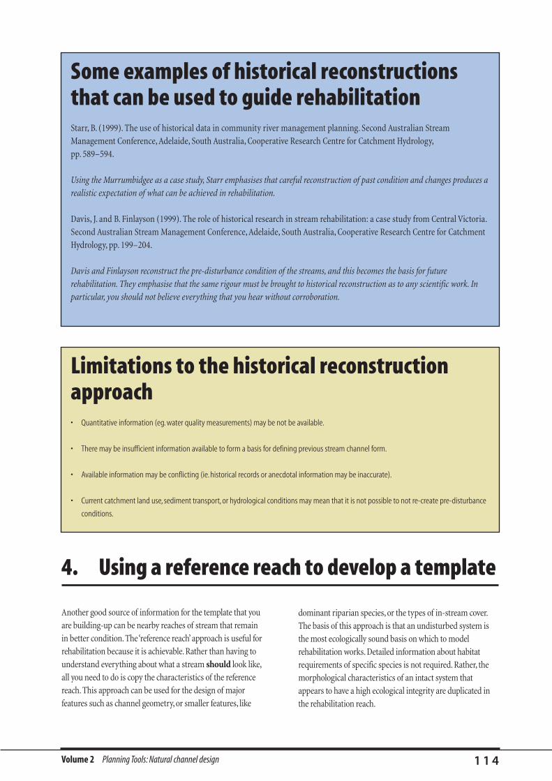
dominant riparian species, or the types of in-stream cover.
The basis of this approach is that an undisturbed system is
the most ecologically sound basis on which to model
rehabilitation works.Detailed information about habitat
requirements of specific species is not required.Rather, the
morphological characteristics of an intact system that
appears to have a high ecological integrity are duplicated in
the rehabilitation reach.
Volume 2 Planning Tools: Natural channel design 1 1 4
Another good source of information for the template that you
are building-up can be nearby reaches of stream that remain
in better condition.The ‘reference reach’ approach is useful for
rehabilitation because it is achievable.Rather than having to
understand everything about what a stream should look like,
all you need to do is copy the characteristics of the reference
reach.This approach can be used for the design of major
features such as channel geometry, or smaller features, like
4. Using a reference reach to develop a template
Some examples of historical reconstructionsthat can be used to guide rehabilitationStarr, B. (1999). The use of historical data in community river management planning. Second Australian Stream
Management Conference, Adelaide, South Australia, Cooperative Research Centre for Catchment Hydrology,
pp. 589–594.
Using the Murrumbidgee as a case study, Starr emphasises that careful reconstruction of past condition and changes produces a
realistic expectation of what can be achieved in rehabilitation.
Davis, J. and B. Finlayson (1999). The role of historical research in stream rehabilitation: a case study from Central Victoria.
Second Australian Stream Management Conference, Adelaide, South Australia, Cooperative Research Centre for Catchment
Hydrology, pp. 199–204.
Davis and Finlayson reconstruct the pre-disturbance condition of the streams, and this becomes the basis for future
rehabilitation. They emphasise that the same rigour must be brought to historical reconstruction as to any scientific work. In
particular, you should not believe everything that you hear without corroboration.
Limitations to the historical reconstructionapproach• Quantitative information (eg. water quality measurements) may be not be available.
• There may be insufficient information available to form a basis for defining previous stream channel form.
• Available information may be conflicting (ie. historical records or anecdotal information may be inaccurate).
• Current catchment land use, sediment transport, or hydrological conditions may mean that it is not possible to not re-create pre-disturbance
conditions.
Volume 2 Planning Tools: Natural channel design 1 1 5
There are, of course, three limitations on the use of
references reaches as templates.
1. If the reference and target reaches should be similar (see
below), why aren’t they? That is, what has caused the
target reach to be different from its original good
condition? Is it something to do with changes in
catchment land use, discharge, erosion, channelisation
or some other stream process? Without addressing the
cause of stream degradation problems, the same forces
may result in failure of the rehabilitation efforts
(Kondolf, 1996). For example, a stream that was
channelised and concrete-lined in response to major
erosion events following urbanisation might be
rehabilitated by removal of the hard lining and
reinstating the previous channel morphology. However,
these works will almost certainly fail due to channel
erosion, because the urban influenced discharge is no
longer in equilibrium with the previous channel form.
As rivers are dynamic in their nature, rehabilitation
measures that are based on a static appraisal of the
river condition can produce uncertain results.
2. The characteristics of the reference reach need to be
scaled to ‘fit’ the target reach. That is, the reference
reach will probably be in a different part of the
catchment, with a different catchment area, discharge
and sediment load, compared with the target reach.You
need to make sure that you scale the size of the
reference to the size of the target reach. This sizing is
normally done on the basis of bankfull discharge. This
scaling is discussed below, and discussed well in
Newbury and Gaboury (1993).
3. This approach is based on the assumption that the
chosen reference reach is stable, is in dynamic
equilibrium, and does support the stream organisms
that you wish to encourage in the target reach. If this is
not the case, then the template you develop for the
target reach is unlikely to be successful.
4.1. Selection of the reference reach
For this template design approach to work, the reference
reach must be a suitable goal for the target reach. That is,
the two reaches should have been similar, until one of
them was disturbed. If the two reaches were never similar,
because of fundamental differences in the character of the
catchment and stream, then it is unlikely that we could
succeed in making them similar now.
When searching for a suitable reference reach, first look for
sites up and downstream of the target reach. If
unsuccessful, look in an adjacent catchment with similar
geology. If unsuccessful, look for the closest catchment that
appears to have similar geological and size characteristics.
In some cases the best template reach can be intact
remnants of the target reach itself. Remnants of modified
channels are often left alongside the target reach in the
form of cut-off meander bends or longer reaches of old
stream. At the very least, these can provide information
about the width and planform of the original channel. In
most Australian streams the dimensions of these relict
channels will not alter much after they have been
abandoned. However, you should check old maps to make
sure that the stream you are looking at is not a relic of a
former hydrological or sediment transport regime
(palaeo-channel). For example, many of the old meanders
flanking the Murray River and other streams of the
Riverine Plains are several times larger than the present
channel, reflecting larger flows that occurred at least
20,000 years ago (Bowler, 1978).
Issues to compare between reference and target reaches
and their catchments are listed in Table 13.
There is no need to fully understand the many processes
operating in the reference reach that seem to produce such ideal
ecological conditions— the objective is simply to copy the
channel form,vegetation,and habitat characteristics in the hope
that the desired ecological processes will become established.
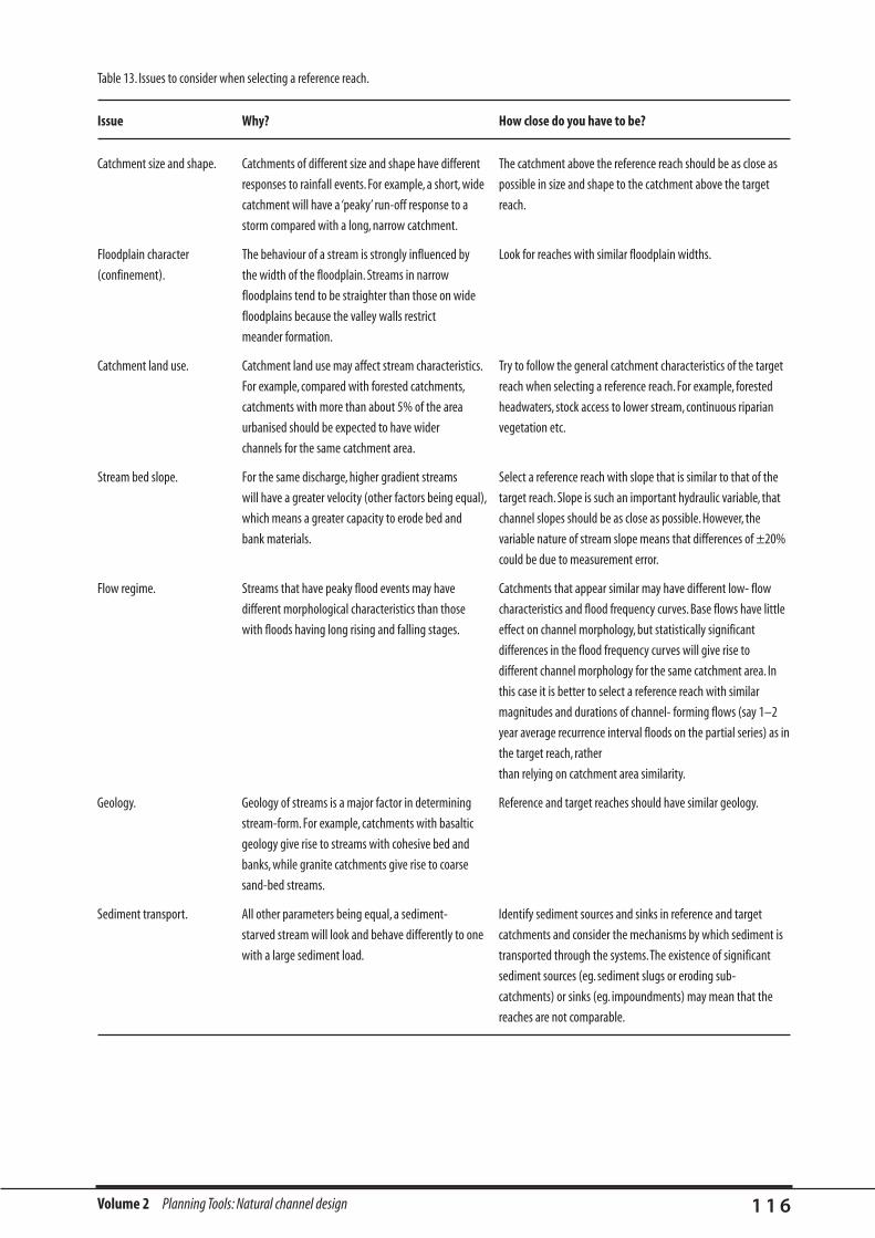
Volume 2 Planning Tools: Natural channel design 1 1 6
Table 13. Issues to consider when selecting a reference reach.
Issue Why? How close do you have to be?
Catchment size and shape. Catchments of different size and shape have different The catchment above the reference reach should be as close as
responses to rainfall events. For example, a short, wide possible in size and shape to the catchment above the target
catchment will have a ‘peaky’ run-off response to a reach.
storm compared with a long, narrow catchment.
Floodplain character The behaviour of a stream is strongly influenced by Look for reaches with similar floodplain widths.
(confinement). the width of the floodplain. Streams in narrow
floodplains tend to be straighter than those on wide
floodplains because the valley walls restrict
meander formation.
Catchment land use. Catchment land use may affect stream characteristics. Try to follow the general catchment characteristics of the target
For example, compared with forested catchments, reach when selecting a reference reach. For example, forested
catchments with more than about 5% of the area headwaters, stock access to lower stream, continuous riparian
urbanised should be expected to have wider vegetation etc.
channels for the same catchment area.
Stream bed slope. For the same discharge, higher gradient streams Select a reference reach with slope that is similar to that of the
will have a greater velocity (other factors being equal), target reach. Slope is such an important hydraulic variable, that
which means a greater capacity to erode bed and channel slopes should be as close as possible. However, the
bank materials. variable nature of stream slope means that differences of ±20%
could be due to measurement error.
Flow regime. Streams that have peaky flood events may have Catchments that appear similar may have different low- flow
different morphological characteristics than those characteristics and flood frequency curves. Base flows have little
with floods having long rising and falling stages. effect on channel morphology, but statistically significant
differences in the flood frequency curves will give rise to
different channel morphology for the same catchment area. In
this case it is better to select a reference reach with similar
magnitudes and durations of channel- forming flows (say 1–2
year average recurrence interval floods on the partial series) as in
the target reach, rather
than relying on catchment area similarity.
Geology. Geology of streams is a major factor in determining Reference and target reaches should have similar geology.
stream-form. For example, catchments with basaltic
geology give rise to streams with cohesive bed and
banks, while granite catchments give rise to coarse
sand-bed streams.
Sediment transport. All other parameters being equal, a sediment- Identify sediment sources and sinks in reference and target
starved stream will look and behave differently to one catchments and consider the mechanisms by which sediment is
with a large sediment load. transported through the systems.The existence of significant
sediment sources (eg. sediment slugs or eroding sub-
catchments) or sinks (eg. impoundments) may mean that the
reaches are not comparable.

Volume 2 Planning Tools: Natural channel design 1 1 7
4.2. Describing the reference reach
The idea of using a reference reach as a template is not to
make the target reach a meticulous precise replica of the
reference reach, down to the position of every tree and the
length of every pool. Rather, it is to recreate to the
character of the reference site—the type of vegetation
present, and the normal size of pools.
The following are some variables that you might measure
when comparing a target and reference reach:
1. catchment conditions;
2. planform character;
3. cross-section information;
4. materials—substrate and banks;
5. slope;
6. vegetation; and
7. biota.
Flow conditions are discussed later.
The best way to decide what to measure is to think about
what you want to do with the data. For example:
• The vegetation may be the only feature of the reference
site that is relevant to the target site, so just describe that.
• If you only want to use the reference reach to provide
some general ideas to display to a stakeholder
consultation committee, then perhaps photographs are
the only information that you need.
• If you are going to use the reference both to design the
target reach, as well as to provide some data against
which you can evaluate later performance, then expect
to do make detailed measurements.
4.2.1 . Catchment conditions
Catchment conditions are the external factors influencing
the template and target reach. The most obvious
descriptions of these are catchment area, bankfull
discharge (if possible), bedrock outcrops, and features
that confine the channel, such as terraces, or floodplain
restrictions. The best way to describe the catchment
conditions is to produce a map of the template and target
catchment with all of the above details marked.
4.2.2. Planform
Planform can be described in detail in terms of
wavelength, arc radius, amplitude and radius of curvature.
Such data can be useful in re-meandering projects, and in
defining buffer zones. These variables can be measured in
the way shown in Figure 4. Usually it is sufficient to
compare the general meander patterns on maps of the
target and template reaches.
Example of thereference reachapproach: NorthPine River,Manitoba (Newburyand Gaboury, 1993)Pine River (Manitoba, Canada) supports rainbow and brook
trout populations. However, sections of North Pine Creek are
steep and shallow due to armouring of the bed with large
rocks and cobbles. In order to increase the trout habitat, one of
these steep sections was selected for stream rehabilitation. A
reference or template reach that had been identified as having
plenty of trout was used as a reference reach.The
characteristics of the pools, riffles and meanders in the
reference reach were then used as design guidelines for
constructing experimental meanders in a straight reach of
North Pine Creek.
You must sample so that your measurements reflect the range
of values found in the reach as well as the average. Often the
range is more important than the average when it comes to
ecological factors.

Volume 2 Planning Tools: Natural channel design 1 1 8
Other information that can be included on the maps
includes:
• in-channel benches;
• point-bars;
• major erosion areas;
• pools;
• riffles;
• artificial levees; and
• vegetation.
4.2.3. Cross-section
The number of cross-sections required to characterise the
channel depends on the degree of variation in the channel
form. The most rigorous way to collect the data is to survey
cross-sections at fixed distances along the channel. This
avoids the temptation to pick out features that could bias
the result. The sampling distance must be chosen to reflect
the size of the channel, and a good rule of thumb is that
you should survey a cross-section every three channel
widths, followed by two widths, then three widths etc. This
sampling approach will pick up any systematic variations,
say in a pool–riffle sequence.
The main features that must be recorded in a survey are:
• degree of channel confinement (width of the floodplain
or other confining feature);
• top-of-bank points on both banks;
• bank slopes;
• width of the active bed; and
• bankfull depth.
Unless you are going to be using these features for detailed
evaluation, they all can be surveyed with a tape and
inclinometer. One of the best ways to survey cross-sections
in small streams is to simply hang a tape or surveying staff
across the channel, check that it is horizontal using a spirit
level, then measure the distance from the tape or staff to
the bed at set distances. Dumpy levels and theodolites can
allow quick collection of accurate data in a short period of
time, but may be difficult to carry in the field. In larger
streams that cannot be easily crossed easily, a range finder
can be used to estimate width.
4.2.4. Slope
Measuring the slope is important for hydraulic design.
This needs to be done with a level or theodolite, as
inclinometers and other hand-held devices are not
accurate enough over tens to hundreds of metres.
Where do you measure slope in a highly variable stream?
Since most channel design uses the bankfull flow and
dimensions, the following are the slope lines that can be
measured, in order of preference.
• Water surface slopes at a range of flow levels (difficult
to measure during flood events).
• Bankfull water surface profile (if you happen to be in the
field when the river is flowing close to bankfull then
survey the water level over a reach of at least 100 metres).
• Slope at top of bank on each side over a reach of at least
100 metres. If possible this should be measured over a
full meander wavelength (ie. three riffles or two bends).
• Bed slope can be even better than bank slope, but only
if it is measured over at least two full meander
Figure 4.Variables used to describe planform of a stream (from
Shields, 1996). Reproduced with permission from
John Wiley & Sons.

Volume 2 Planning Tools: Natural channel design 1 1 9
wavelengths (to smooth out the many variations in the
bed). Bed slope should be measured along the thalweg
or centre line of flow.
4.2.5. Bed and bank material
Bank material needs to be described in order to check that
the template and target reaches are similar. It is usually
sufficient to simply classify the bank material as fine or
coarse gravel, sand, silt and loam, clay, or a combination of
these. The layers of material should be drawn on each
cross-section with the thickness of the units indicated.
The particle size distribution of the bed material can also be
important.A change in substrate may well be one of the
goals of the rehabilitation project.Also, we need to know
about bed material for channel design (equations often use
median bed material size). The Wolman pebble count
method (Kellerhals, 1971) is appropriate for gravel bed
streams, while sieving is required for finer bed material. The
technique is to simply shut your eyes (or just look away),
reach down to the bed and touch it with your finger. Pick up
the very first particle that you touched and measure its ‘B’
axis (ie. that axis that it would roll along on the bed). Take a
step, shut your eyes again, and touch another pebble, and
measure it. Do this 100 times on a mid-channel bar, or in
the bed of the stream. It is important that you do not look!
4.2.6. Vegetation
Vegetation surveys are aided by identifying the ‘zone’ of the
cross-section that is occupied by different vegetation
types. Some excellent examples of this are provided in the
booklets by Allan Raine and others (eg. Raine and
Gardiner, 1997). Figure 5 shows an example of the species
that are found on different parts of the bank in a template
stream.You may even want to be more specific and
identify plants growing on specific depositional sites
within the cross-section such as benches, point-bars, and
mid-channel bars.
4.2.7. Biota
A survey of the mammals, birds, fish, and
macroinvertebrates living in the template reach is
invaluable as a reference for the target reach, but is also
very expensive and time-consuming to do. Two easier
things that are often worth doing are a presence or absence
survey of fish (fishing clubs can provide this information)
and macroinvertebrates. Alternatively, a survey of fish
could be done using electro-fishing techniques. This
technique takes about one day per 100–200 m reach. See
Biological site assessment of stream health, in Catchment
review (this volume), for some more ideas on surveying
the stream biota.
Larger trees with deep root systems
Stream
Low-growing, multi-trunkedplants with matted roots to bind the toe
Medium sized plants with good root systems and larger canopies which shade the stream
Figure 5.The different types of plants that can be found on different zones of the stream bank (from Raine and Gardiner, 1997).
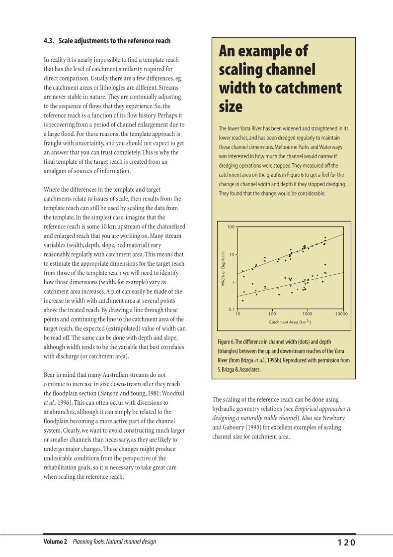
An example ofscaling channelwidth to catchmentsizeThe lower Yarra River has been widened and straightened in its
lower reaches, and has been dredged regularly to maintain
these channel dimensions. Melbourne Parks and Waterways
was interested in how much the channel would narrow if
dredging operations were stopped.They measured off the
catchment area on the graphs in Figure 6 to get a feel for the
change in channel width and depth if they stopped dredging.
They found that the change would be considerable.
Volume 2 Planning Tools: Natural channel design 1 2 0
4.3. Scale adjustments to the reference reach
In reality it is nearly impossible to find a template reach
that has the level of catchment similarity required for
direct comparison. Usually there are a few differences, eg.
the catchment areas or lithologies are different. Streams
are never stable in nature. They are continually adjusting
to the sequence of flows that they experience. So, the
reference reach is a function of its flow history. Perhaps it
is recovering from a period of channel enlargement due to
a large flood. For these reasons, the template approach is
fraught with uncertainty, and you should not expect to get
an answer that you can trust completely. This is why the
final template of the target reach is created from an
amalgam of sources of information.
Where the differences in the template and target
catchments relate to issues of scale, then results from the
template reach can still be used by scaling the data from
the template. In the simplest case, imagine that the
reference reach is some 10 km upstream of the channelised
and enlarged reach that you are working on. Many stream
variables (width, depth, slope, bed material) vary
reasonably regularly with catchment area. This means that
to estimate the appropriate dimensions for the target reach
from those of the template reach we will need to identify
how those dimensions (width, for example) vary as
catchment area increases.A plot can easily be made of the
increase in width with catchment area at several points
above the treated reach. By drawing a line through these
points and continuing the line to the catchment area of the
target reach, the expected (extrapolated) value of width can
be read off. The same can be done with depth and slope,
although width tends to be the variable that best correlates
with discharge (or catchment area).
Bear in mind that many Australian streams do not
continue to increase in size downstream after they reach
the floodplain section (Nanson and Young, 1981; Woodfull
et al., 1996). This can often occur with diversions to
anabranches, although it can simply be related to the
floodplain becoming a more active part of the channel
system. Clearly, we want to avoid constructing much larger
or smaller channels than necessary, as they are likely to
undergo major changes. These changes might produce
undesirable conditions from the perspective of the
rehabilitation goals, so it is necessary to take great care
when scaling the reference reach.
The scaling of the reference reach can be done using
hydraulic geometry relations (see Empirical approaches to
designing a naturally stable channel). Also see Newbury
and Gaboury (1993) for excellent examples of scaling
channel size for catchment area.
100.1
1
10
100
2
100
Catchment Area (km )
Wid
th o
r D
epth
(m)
1000 10000
Figure 6.The difference in channel width (dots) and depth
(triangles) between the up and downstream reaches of the Yarra
River (from Brizga et al., 1996b).Reproduced with permission from
S.Brizga & Associates.

Volume 2 Planning Tools: Natural channel design 1 2 1
4.4. Limitations of the template approach
One overall criticism of the template approach was made
by the US National Research Council (1992).
"When stream or river management actions are taken
without recognising whether the aquatic ecosystem is in
dynamic equilibrium or disequilibrium, the manager is
gambling with the stream or river rather than ensuring
improved ecosystem function and dynamic stability. The
well-intentioned but intuitive [template] approach may
therefore cause unexpected harm even to species that
were meant to be helped."
Specific limitations of the template approach are:
• the difficulty in ensuring similar land use, geology,
slope, sediment transport and storage and flood
conditions between reference and target reaches;
• dubious accuracy of scaling channel morphological
features by extrapolation; and
• identifying a suitable reference reach is likely to be
difficult in many areas of Australia because of the high
level of catchment disturbance. This is particularly true
of lowland streams.
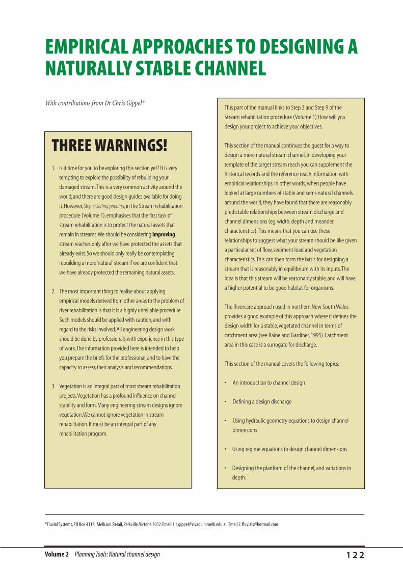
With contributions from Dr Chris Gippel*
Volume 2 Planning Tools: Natural channel design 1 2 2
EMPIRICAL APPROACHES TO DESIGNING ANATURALLY STABLE CHANNEL
This part of the manual links to Step 3 and Step 9 of the
Stream rehabilitation procedure (Volume 1) How will you
design your project to achieve your objectives.
This section of the manual continues the quest for a way to
design a more natural stream channel. In developing your
template of the target stream reach you can supplement the
historical records and the reference reach information with
empirical relationships. In other words, when people have
looked at large numbers of stable and semi-natural channels
around the world, they have found that there are reasonably
predictable relationships between stream discharge and
channel dimensions (eg. width, depth and meander
characteristics).This means that you can use these
relationships to suggest what your stream should be like given
a particular set of flow, sediment load and vegetation
characteristics.This can then form the basis for designing a
stream that is reasonably in equilibrium with its inputs.The
idea is that this stream will be reasonably stable, and will have
a higher potential to be good habitat for organisms.
The Rivercare approach used in northern New South Wales
provides a good example of this approach where it defines the
design width for a stable, vegetated channel in terms of
catchment area (see Raine and Gardiner, 1995). Catchment
area in this case is a surrogate for discharge.
This section of the manual covers the following topics:
• An introduction to channel design
• Defining a design discharge
• Using hydraulic geometry equations to design channel
dimensions
• Using regime equations to design channel dimensions
• Designing the planform of the channel, and variations in
depth.
THREE WARNINGS!1. Is it time for you to be exploring this section yet? It is very
tempting to explore the possibility of rebuilding your
damaged stream.This is a very common activity around the
world, and there are good design guides available for doing
it.However, Step 5: Setting priorities, in the Stream rehabilitation
procedure (Volume 1),emphasises that the first task of
stream rehabilitation is to protect the natural assets that
remain in streams.We should be considering improving
stream reaches only after we have protected the assets that
already exist.So we should only really be contemplating
rebuilding a more ‘natural’stream if we are confident that
we have already protected the remaining natural assets.
2. The most important thing to realise about applying
empirical models derived from other areas to the problem of
river rehabilitation is that it is a highly unreliable procedure.
Such models should be applied with caution,and with
regard to the risks involved.All engineering design work
should be done by professionals with experience in this type
of work.The information provided here is intended to help
you prepare the briefs for the professional,and to have the
capacity to assess their analysis and recommendations.
3. Vegetation is an integral part of most stream rehabilitation
projects.Vegetation has a profound influence on channel
stability and form.Many engineering stream designs ignore
vegetation.We cannot ignore vegetation in stream
rehabilitation. It must be an integral part of any
rehabilitation program.
*Fluvial Systems, PO Box 4117, Melb.uni.Retail, Parkville,Victoria 3052. Email 1:[email protected] Email 2: [email protected]

Volume 2 Planning Tools: Natural channel design 1 2 3
The concept of regime channels began in the 19th century
as British engineers were designing and building canals in
Pakistan and India (Chang, 1988). The basis for regime
theory was to describe a cross-sectional geometry for
designing equilibrium or ‘regime’ canals. At any point on
the canal, it was regarded as being in ‘regime’ if there was
no net aggradation or degradation at that point for a given
design discharge. The equations that described this
condition were called regime equations.
In the 1960s, Leopold, Wolman and Miller in the US, and
others, noted that there were reasonably consistent
relationships between the discharge carried by a natural
stream, its sediment character, its catchment area and the
size, shape and slope of the channel. They developed what
they called ‘at-a-station’ hydraulic geometry relationships
to describe how the cross-section width and depth
changed as discharge increased. These relationships were
very similar to the regime equations.
Hydraulic geometry also has a catchment-wide
perspective. Relationships were derived to characterise, on
a catchment-wide basis, how channel morphology
changed with increasing discharge downstream, or
increasing catchment area downstream. These are known
as ‘downstream’ hydraulic geometry relationships. Later
work built on this approach by including other natural
channel features such as meander form and pool riffle
spacing. Downstream hydraulic geometry relationships are
usually simple, in that they predict channel morphology
anywhere in a catchment (it is a regional-scale approach)
on the basis of only catchment area or channel-forming
discharge (or some other convenient discharge index),
although some models are more complex and incorporate
other variables. Regime equations predict channel
morphology at a point (it is a channel reach approach) on
the basis of a design discharge, and sometimes combined
with the size of the material making up the bed and banks.
The empirical catchment or channel model approach to
stream rehabilitation contends that within certain error
bands, it should be possible to predict, or reconstruct a
channel form that is in dynamic equilibrium with its
discharge. This approach should be used in conjunction
with other approaches to stream rehabilitation. Before the
analysis is carried out, it is necessary to have an
understanding of the catchment and river processes that
are occurring.
The empirical catchment and channel model method for
stream rehabilitation design is based on the premise that
we understand the fluvial system well enough to be able to
design a stream that would be dynamically stable under
natural conditions. This approach is most successful in
determining the broad geometry of streams in terms of
the average width and depth of the stream, and is less
successful at determining habitat requirements, like the
proportion or type of cover suitable for a particular fish
species.
The empirical downstream hydraulic geometry models of
how channels change their morphology as discharge or
catchment area increases are misleading because they
rarely track the downstream change along a particular
stream channel. The sample points are usually distributed
all over the catchment. This partially explains the scatter in
the relationships.Along the path of an individual stream,
the channel morphology is likely to change dramatically
only at points of major changes in discharge—at tributary
junctions. Between the tributary junctions the channel is
likely to be relatively constant (apart from the normal
oscillations due to pools and riffles and variations in bank
material and vegetation). Rehabilitation projects usually
consider continuous, or linked reaches of streams, so it is
this step-like downstream change that is more relevant to
rehabilitation design.
The empirical model approach is especially unreliable in
Australia for three main reasons. The first is that most
available models of hydraulic geometry and regime were
developed overseas in streams that we either know very
little about, or we know are very different from natural
streams found in Australia. The second reason is that
Australian streams are typically very different
hydrologically and geomorphologically to streams in the
northern hemisphere. The flow in Australian rivers is
usually much more variable, so it is less likely that they are
adjusted to a flow of a particular recurrence interval.
Rather they may simply reflect the time series of discharge
(flow history), with the morphology largely reflecting the
timing and magnitude of the most recent catastrophic
event. Geomorphologically, Australian rivers drain
1. An introduction to the empirical approach to channel design

To understand the concept of a dominant discharge, we
must understand the relationship between a river and its
floodplain. When a river deposits sediment it tends to
form relatively flat, horizontally orientated surfaces. We
adopt the following definitions for these surfaces:
Floodplain: a reasonably continuous surface that is
flooded annually, or at least every few years. This surface
has been deposited by the present stream.
Bench: a discontinuous surface that tends to be flooded
more frequently than the active floodplain.
Terrace: a surface above the floodplain that is flooded only
rarely. It was probably deposited in the past. Often it is a
former floodplain that has been isolated by stream incision.
Channel-forming flow is considered to be that flow
responsible for deposition on the present floodplain. The
active floodplain is identified as undergoing net growth
over the current stage of the river morphology (Wharton,
1992) and can be identified as freshly deposited material
such as a flat deposit within an incised channel or a wider
floodplain outside the confines of the channel. The stage of
the channel-forming flow, when water depth just reaches
the level of the active floodplain, is also referred to as the
dominant or bankfull flow. This bankfull flow condition is
the most common design flow used when applying the
analytical or regime approaches.
Although we use the notion of a dominant discharge in
this manual, the notion of a single channel-forming flow is
controversial.
Given that flood flows of a moderate magnitude and
duration seem to be responsible for channel formation,
what changes in the catchment might cause the size of
A key factor for the design of any in-stream structures,
and generally for natural channel design, is to select a
discharge on which to base the design. When installing an
artificial riffle, how do we know how big the rocks should
be so that they are not washed away by floods? One
commonly adopted principle is to use a tractive stress
calculation, such that the tractive stress during bankfull
flow is less than that required to move the rocks. Another
example may be the selection of an equilibrium channel
width for channel realignment.Bankfull discharge or some
surrogate is usually adopted as the design discharge for
regime equations. Bankfull discharge is typically used as
the design flow for in-stream rehabilitation work (not
engineering structures like bridges and culverts).
2.1 . Why bankfull? A discussion of bankfull,dominant and channel-forming flows
The computational approach to channel design is based on
the relationship of bankfull or dominant flow of a stream
and the channel width, depth and slope. The basis of this
approach is that major channel-forming activity (erosion
and depositional events affecting the long-term form of
the bed and banks) occurs during regular (1–2 year)
flooding events. The argument is that channels are
continually going through destruction and recovery
phases, where major floods cause larger-scale channel
modification, which is in turn stabilised over subsequent
years by the channel-forming flow. Another way of
describing the dominant discharge is that it is a single flow
that would produce the same channel form as the full
range of flows that occur in nature. The basis of using
channel-forming flow for channel design is to produce a
quasi-equilibrium channel formation similar to that which
would naturally develop under similar watershed
conditions (Shields, 1996).
catchments that are less steep, have lower sediment yields,
and transport sediment of a finer particle size than
northern hemisphere streams. The final reason is that
Australian streams are known to sometimes display an
erratic downstream pattern of morphological change.
They may effectively disappear into a flood-out, or they
may narrow as they enter the floodplain reaches.
Now that you are aware of the basis and risks of the design
approaches, it is time to look at how the design procedure
can work. The first thing that is required is a design
discharge. This is the foundation of the design procedure.
The design discharge indicates the dimensions and basic
structure of the channel. Once you have the design
discharge, you can use the hydraulic geometry regime
approaches to decide on the design dimensions of the
channel. The design discharge that is usually used for
stream rehabilitation design is the bankfull flow. This flow,
and ways to determine it are discussed in some detail in
the next section.
Volume 2 Planning Tools: Natural channel design 1 2 4
2. Selecting a design discharge
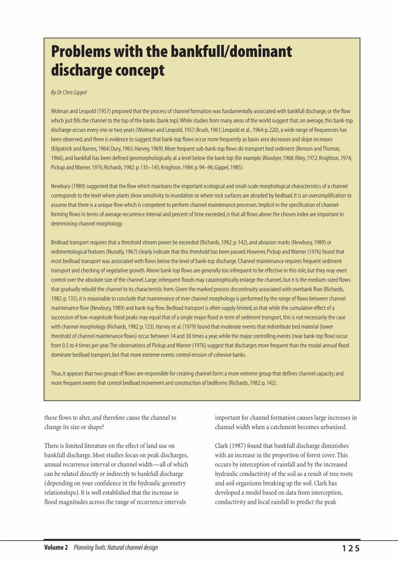
Volume 2 Planning Tools: Natural channel design 1 2 5
these flows to alter, and therefore cause the channel to
change its size or shape?
There is limited literature on the effect of land use on
bankfull discharge. Most studies focus on peak discharges,
annual recurrence interval or channel width—all of which
can be related directly or indirectly to bankfull discharge
(depending on your confidence in the hydraulic geometry
relationships). It is well established that the increase in
flood magnitudes across the range of recurrence intervals
important for channel formation causes large increases in
channel width when a catchment becomes urbanised.
Clark (1987) found that bankfull discharge diminishes
with an increase in the proportion of forest cover. This
occurs by interception of rainfall and by the increased
hydraulic conductivity of the soil as a result of tree roots
and soil organisms breaking up the soil. Clark has
developed a model based on data from interception,
conductivity and local rainfall to predict the peak
Problems with the bankfull/dominantdischarge conceptBy Dr Chris Gippel
Wolman and Leopold (1957) proposed that the process of channel formation was fundamentally associated with bankfull discharge, or the flow
which just fills the channel to the top of the banks (bank top).While studies from many areas of the world suggest that, on average, this bank-top
discharge occurs every one or two years (Wolman and Leopold, 1957; Brush, 1961; Leopold et al., 1964: p. 220), a wide range of frequencies has
been observed, and there is evidence to suggest that bank-top flows occur more frequently as basin area decreases and slope increases
(Kilpatrick and Barnes, 1964; Dury, 1965; Harvey, 1969). More frequent sub-bank-top flows do transport bed sediment (Benson and Thomas,
1966), and bankfull has been defined geomorphologically at a level below the bank top (for example,Woodyer, 1968; Riley, 1972; Knighton, 1974;
Pickup and Warner, 1976; Richards, 1982: p. 135–145; Knighton, 1984: p. 94–96; Gippel, 1985).
Newbury (1989) suggested that the flow which maintains the important ecological and small-scale morphological characteristics of a channel
corresponds to the level where plants show sensitivity to inundation or where rock surfaces are abraded by bedload. It is an oversimplification to
assume that there is a unique flow which is competent to perform channel maintenance processes. Implicit in the specification of channel-
forming flows in terms of average recurrence interval and percent of time exceeded, is that all flows above the chosen index are important in
determining channel morphology.
Bedload transport requires that a threshold stream power be exceeded (Richards, 1982: p. 142), and abrasion marks (Newbury, 1989) or
sedimentological features (Nunally, 1967) clearly indicate that this threshold has been passed. However, Pickup and Warner (1976) found that
most bedload transport was associated with flows below the level of bank-top discharge. Channel maintenance requires frequent sediment
transport and checking of vegetative growth. Above bank-top flows are generally too infrequent to be effective in this role, but they may exert
control over the absolute size of the channel. Large, infrequent floods may catastrophically enlarge the channel, but it is the medium-sized flows
that gradually rebuild the channel to its characteristic form. Given the marked process discontinuity associated with overbank flow (Richards,
1982: p. 135), it is reasonable to conclude that maintenance of river channel morphology is performed by the range of flows between channel
maintenance flow (Newbury, 1989) and bank-top flow. Bedload transport is often supply limited, so that while the cumulative effect of a
succession of low-magnitude flood peaks may equal that of a single major flood in term of sediment transport, this is not necessarily the case
with channel morphology (Richards, 1982: p. 123). Harvey et al. (1979) found that moderate events that redistribute bed material (lower
threshold of channel maintenance flows) occur between 14 and 30 times a year, while the major controlling events (near bank-top flow) occur
from 0.5 to 4 times per year.The observations of Pickup and Warner (1976) suggest that discharges more frequent than the modal annual flood
dominate bedload transport, but that more extreme events control erosion of cohesive banks.
Thus, it appears that two groups of flows are responsible for creating channel form: a more extreme group that defines channel capacity; and
more frequent events that control bedload movement and construction of bedforms (Richards, 1982: p. 142).
catchment comparisons, and to ensure consistency
between stream managers. The following criteria for
identifying bankfull level have been selected from
Australian Rainfall and Runoff (Pilgrim, 1987).
• "If no benches exist, use the floodplain level or, if a
floodplain is not developed, use the edge of the channel
where this is formed by deposition of sediments."
• "If three benches or two definite benches at medium to
high stage exist, use the top bench level."
• "If no one bench exits, proceed as follows:
a) select bankfull level by comparisons with the level at
which the nose of the points of the bend upstream
and downstream flatten out.
b) Confirm this by examining the sediments at this
level for evidence of numerous recent episodes of
deposition, (ie. laminations, flood debris, artefacts
etc.) and by seeking information from local
landholders regarding frequency of flooding."
• "Where necessary, correlate bankfull levels identified at
bends with bankfull levels in straight reaches by
running levels between the bends."
• "Bankfull level is taken to be representative of the
bench or floodplain surface chosen. The level is taken
as near as possible to the stream where the floodplain
surface flattens out."
2.3. Using Manning’s equation to predict thebankfull discharge
Manning’s equation is the most common way of
estimating the bankfull discharge. The steps required to
predict discharge using Manning’s equation are:
• measure channel width and depth and collect data to
be able to calculate the cross-sectional area of at least
five cross-sections in the reach;
• measure the channel slope (bed slope is suitable);
• estimate Manning’s n value (see Table 15); and
• calculate bankfull discharge.
discharge of various land uses. The results of the model
showed that the flood which occurs on average one every
two years had a discharge close to the bankfull discharge
which had been measured in the field. The bankfull
discharge for a catchment under 100% forest cover
increased by 2.5 times when forest was reduced to 80%
cover, by 3 times when forest was reduced to 50% cover,
and by 3.5 times when forest was converted entirely to
pasture. These estimates are very large and must be
considered maximum effects.
Regime equations ignore the real complexity of the
channel forming process—remember they were originally
derived for the design of trapezoidal irrigation canals with
constant discharge! It is this fundamental problem
(assumption of a single dominant discharge) that makes
this approach difficult to apply to natural channel design.
Despite this, it is currently the best approach for routine
channel design. We recommend its use until a better
approach is developed. The following section discusses
ways to estimate the bankfull flow.
2.2. Estimating the bankfull flow
Bankfull flow can be estimated in three ways:
1. by measurement;
2. by estimating the discharge using an equation; and
3. by estimating flood frequency (ie. the 1–2 year flood).
The following sections will describe these methods. To
apply the first two methods you must define a bankfull
point in the channel.
2.2.1. Identifying the bankfull point in the field
Given that bankfull is the level of water in the channel, just
before the water flows out into the floodplain, how do we
measure it? Anyone who has stood on a stream bank
looking for textbook geomorphic features knows how
frustrating it can be to identify the bankfull level. In reality
the channel cross-section is often not easily defined, as
illustrated in Table 14.
Bankfull flow can be defined in several different ways. Any
of these is appropriate, but the key is to be able to
consistently identify bankfull levels to enable inter-
Volume 2 Planning Tools: Natural channel design 1 2 6

Volume 2 Planning Tools: Natural channel design 1 2 7
Manning’s equation for mean velocity is:
where:
v = depth averaged flow velocity (m/s);
R = hydraulic radius (m), which is the cross-sectional area
‘A’ divided by the wetted perimeter ‘P’. The wetted
perimeter for a rectangular channel is 2 times the depth
(y) plus the width (w). For wide channels (where y > about
10 times w) the hydraulic radius can be approximated by
the depth;
S = energy slope or water surface slope, adopted as the
stream bed slope for steady uniform flow; and
n = Manning’s roughness coefficient which is discussed in
the paragraphs to follow.
vR S
n=
( / ) ( / )2 3 1 2
1) The floodplain level occurs at a different height on either side of the stream, so
there is an upper and lower possible bankfull dimension. An average value can
be used.
2) A convex slope may mark the transition from channel wall to floodplain so it is
difficult to decide where to position the bankfull stage.
3) Levee banks higher than the adjoining floodplain will give a larger bankfull
capacity than if the level of the floodplain is adopted as bankfull
4) Compound channel cross-sections (a number of terrace levels usually created
through channel incision), make selection of the correct floodplain terrace
difficult.
5) Severely incised streams and gullies probably never fill to the ‘bankfull’ stage, so
the application of a bankfull design flow to these streams is dubious.
(1)
(2)
(3)
(5)
(4)
Bench
��
Table 14. Situations where the bankfull stage is hard to define.
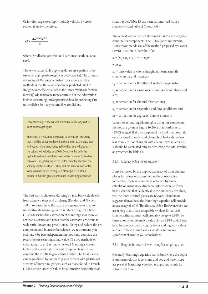
Volume 2 Planning Tools: Natural channel design 1 2 8
Or for discharge, we simply multiply velocity by cross-
sectional area—therefore;
where Q = discharge (m3/s) and A = cross sectional area
(m2).
The key to successfully applying Manning’s equation is the
use of an appropriate roughness coefficient (n). The primary
advantage of Manning’s equation over more analytical
methods is that the value of n can be predicted quickly.
Roughness coefficients such as the Darcy-Weisbach friction
factor (f) will tend to be more accurate, but their derivation
is time-consuming, and appropriate data for predicting f are
not available for many natural flow conditions.
stream types. Table 15 has been summarised from a
frequently cited table of Chow, 1959).
The second way to predict Manning’s n is to estimate, then
combine, its components. The USDA (Gore and Bryant,
1988) recommends use of the method proposed by Cowan
(1956) to estimate the value of n:
n = (n0
+ n1
+ n2
+ n3
+ n4)m
where:
n0
= base value of n for a straight, uniform, smooth
channel in natural materials;
n1
= correction for the effect of surface irregularities;
n2
= correction for variations in cross-sectional shape and
size;
n3
= correction for channel obstructions;
n4
= correction for vegetation and flow conditions; and
m = correction for degree of channel sinuosity.
Values for estimating Manning’s n using this component
method are given in Figure 16. Note that Gordon et al.
(1992) suggest that the component method is appropriate
only for small to mid-sized channels of hydraulic radius
less than 5 m. For channels with a larger hydraulic radius,
n should be calculated only by predicting the total n value,
as presented in Table 15.
2.3.1. Accuracy of Manning’s equation
Don’t be misled by the implied accuracy of three decimal
places for values of n presented in the above tables.
Remember, these n values were obtained by back-
calculation using stage discharge information, so if you
have a channel that is identical to the one measured then,
yes, the three decimal places are relevant. Henderson
suggests that, at best, the Manning’s equation will provide
an accuracy of ±1% (Henderson, 1966). However, when we
are trying to estimate acceptable n values for natural
channels, this variation will probably be up to ±10%. So
think about your estimated value of n as ±10% and, if you
have time, recalculate using the lower and higher n values
and see if these revised values would result in any
significant change in your conclusions.
2.3.2. Things to be aware of when using Manning’s equation
Generally, Manning’s equation works best where the depth
is uniform, velocity is constant, and bed and water slope
are parallel. Manning’s equation is appropriate only for
sub-critical flows.
Since Manning’s n seems such a small number, why is it so
important to get right?
Manning’s n is raised to the power of one (ie. n1), meaning
that it will be directly reflected in the answer to the equation;
ie. if you vary Manning’s n by ±10% then you will also vary
the calculated velocity by ±10%. Compare this with the
hydraulic radius R, which is raised to the power of 2/3—less
than one.Thus, if R is varied by ±10% then the effect on the
velocity will be less than ±10%, and the same is true for the
slope which is raised to only 1/2. Although n is a small
number it has the greatest influence in Manning’s equation.
QAR S
n=
( / ) ( / )3 2 1 2
The best way to choose a Manning’s n is to back-calculate it
from a known stage and discharge (Kondolf and Micheli,
1995). We rarely have the luxury of a gauged reach, so we
must estimate Manning’s n from tables or figures. Chow
(1959) describes the estimation of Manning’s n as more an
art than a science and notes that the estimates are prone to
wide variation among practitioners. To try and reduce the ‘art’
component and increase the ‘science’, we recommend you
estimate n by two independent methods and compare the
results before selecting a final value. The two methods of
estimating n are: 1) estimate the total Manning’s n from
tables; and 2) estimate different components of n then
combine the results to give a final n value. The total n value
can be predicted by comparing your stream with pictures of
streams of known roughness, such as those found in French
(1986), or use tables of values for alternative descriptions of

Volume 2 Planning Tools: Natural channel design 1 2 9
• Estimates of Manning’s n are subjective, so that if five
stream managers are each asked to estimate a
Manning’s n you may get five different numbers.
• Channel roughness varies with depth. For example, as
flow depth increases with discharge, the influence
that debris located towards the bed of the channel
has on the flow resistance decreases. Gregory et al.
(1985) observed a reduction in n from an extremely
high value of 1.02 at low flows to 0.31 as the flow
increased in an upland stream in the UK. Estimated
values of Manning’s n should be based on a design
flow depth.
• The roughness of very weedy and vegetation-choked
channels can be very high, especially at low flows; n
values of 1.0 are common.
• In some cases, the value of n has been found to increase
with stage. For example, Petryk and Bosmajian (1975)
found that in channels that are heavily obstructed by
trees and debris the density of obstructions remained
roughly constant with rising stage and that the value of
Manning’s n actually increased with discharge.
• It has been suggested (Gippel et al., 1992) that Manning’s
n is not a suitable measure of the roughness provided by
a channel with a significant in-stream obstruction
component. For example, Gippel et al. (1996b) considered
that the contribution of in-channel debris to a channel’s
roughness depends on many factors including the size
and shape of the channel, the stage of the flow, bank
irregularities and the degree of meandering. Manning’s
equation was developed for open-channel flow
conditions, where the retardation of the flow is primarily
controlled by bed roughness elements. In a heavily
congested channel the concept of hydraulic radius, on
which Manning’s relies, may become meaningless. There
are, nevertheless, no straightforward alternatives to
Manning’s n for this situation.
Design flow estimation for the Acheron Riverusing Manning’s equationThe Acheron River is in central eastern Victoria. At the point where we wish to estimate the design flow, the catchment area is about 500 km2.
Five cross-sections using a line level and staff were surveyed within the target reach.We are interested in water surface slope at bankfull flow.
This can be estimated from the bed slope, but a better approximation is the top of the bank itself—it tends to be less variable than the bed.Top-
of-bank slope was measured using a level for the entire 400 m length of the reach.The surveyed slope was 0.0018, the estimated Manning’s n for
the reach was 0.04. Manipulated data are presented in Table 17.
Table 17.The data used to calculate the Acheron River design flow using Manning’s equation.
Cross- section discharge Bankfull width Bankfull depth (average) Cross-sectional area Bankfull (m3/s)
1 17.2 1.48 25.5 31.6
2 16.5 1.38 22.8 27.1
3 15 1.55 23.9 30.5
4 14 1.86 24.7 32.7
5 16.1 1.60 25.8 33.3
Details from these five cross-sections indicate that the bankfull discharge at this reach is about 31 m3/s.

Volume 2 Planning Tools: Natural channel design 1 3 0
Channel type Range Normal
ARTIFICIAL STREAMS:
Lined or built-up channels
Concrete 0.011–0.025 0.015
Concrete bottom, float 0.015–0.035 0.025
finished with stone sides
Gravel bottom with 0.017–0.026 0.020
concrete sides
Gravel bottom with 0.023–0.036 0.035
riprap sides
Artificial streams: unlined
A) Earth, straight and uniform
1) Clean 0.018–0.025 0.022
2) With short grass, 0.022–0.033 0.027
few weeds
B) Earth, winding and sluggish
1) No vegetation 0.023–0.030 0.025
2) Grass, some weeds 0.025–0.033 0.030
3) Dense weeds or aquatic 0.030–040 0.035
plants in deep channels
4) Earth bottom and rubble sides 0.028–0.035 0.030
5) Stony bottom and weedy banks 0.025–0.040 0.035
6) Cobble bottom and clean sides 0.030–0.050 0.040
C) Unmaintained channels
1) dense weeds as high 0.050–0.120 0.080
(ie. heavy foliage)
2) clean bottom brush on sides 0.040–0.080 0.050
3) Same as above at highest stage 0.045–0.110 0.070
of flow
4) Dense brush, high stage 0.080–0.140 0.100
NATURAL STREAMS:
Minor streams
(top width at flood stage <33 m)
A) Streams on plain
1) Clean, straight, full stage, 0.025–0.033 0.030
no rifts or deep pools
2) Same as above, but more 0.030–0.40 0.035
stones and weeds
Channel type Range Normal
3) Clean, winding, some 0.033–0.045 0.040
pools and shoals
4) Same as above, but 0.035–0.050 0.045
some weeds and stones
5) Same as above, lower 0.040–0.055 0.048
stages, more ineffective
slopes and sections
6) Same as no. 4, more stones 0.045–0.060 0.050
7) Sluggish reaches, weedy, 0.050–0.080 0.070
deep pools
8) Very weedy reaches, deep pools, 0.075–0.150 0.100
or floodways with heavy stand
of timber and underbrush
B) Mountain streams, no vegetation in channel, banks usually
steep, trees and brush along banks submerged at high stages
1) Bottom: gravels, cobbles, and 0.030–0.050 0.040
few boulders
2) Bottom: cobbles with large boulders 0.040–0.070 0.050
Floodplains
A) Pasture, no brush
1) Short grass 0.025–0.035 0.030
2) High grass 0.030–0.050 0.035
3) Mature field crop 0.030–0.050 0.040
B) Cultivated Areas
1) No crop 0.020–0.040 0.030
2) Mature row crop 0.025–0.045 0.035
3) Mature Field crop 0.030–0.050 0.040
C) Brush
1) Scattered brush, heavy weeds 0.035–0.070 0.050
2) light brush and trees, in winter 0.035–0.060 0.050
(ie. low foliage)
3) Light brush and trees, in summer 0.040–0.080 0.060
(ie. heavy foliage)
4) Medium to dense brush, in winter
(ie. light foliage) 0.045–0.110 0.070
5) medium to dense brush, in summer 0.070–0.160 0.100
(ie. heavy foliage)
Table 15.Table of total n values summarised from Chow (1959) as presented in French (1986).

Volume 2 Planning Tools: Natural channel design 1 3 1
Table 16.Values for estimation of Manning’s n, from Zipparro and Hasen (1993).
Channel conditions Values
Material involved Earth 0.020
Rock cut n0 0.025
Fine gravel 0.024
Coarse gravel 0.028
Degree of irregularity Smooth 0.000
Minor n1 0.005
Moderate 0.010
Severe 0.020
Variations of channel cross-section Gradual 0.000
Alternating occasionally n2 0.005
Alternating frequently 0.010–0.015
Relative effect of obstructions Negligible 0.000
Minor n3 0.010–0.015
Appreciable 0.020–0.030
Severe 0.040–0.060
Vegetation Low 0.005–0.010
Medium n4 0.010–0.025
High 0.025–0.050
Very high 0.050–0.100
Degree of meandering Minor (sinuosity 1.0–1.2) 1.000
Appreciable (sinuosity 1.2–1.5) m 1.150
Severe (sinuosity >1.5) 1.300
Channel type Range Normal
D) Trees
1) Dense willows, straight, summer 0.110–0.200 0.150
(dense vegetation)
2) Cleared land with tree stumps,
no sprouts
3) Same as above, but with heavy 0.050–0.080 0.060
growth of sprouts
4) heavy stand of timber, a 0.080–0.120 0.100
few down trees, little
undergrowth, flood stage
below branches
Table 15 (cont’d).Table of total n values summarised from Chow (1959) as presented in French (1986).
Channel type Range Normal
5) same as above but with flood 0.100–0.160 0.120
stage reaching branches
Major streams
Top width at flood stage >
33 m—the n value is less than
that for minor streams of similar
description because the banks
offer less effective resistance
A) Regular cross-section with 0.025–0.060
no boulders or brush
B) Irregular and rough section 0.035–0.100
Volume 2 Planning Tools: Natural channel design 1 3 2
2.4 . Using flood frequency analysis to predict thebankfull discharge
A common way to check the design discharge (ie. the
bankfull or dominant discharge) is to use flood frequency
analysis to predict the size of the flood with the return
interval of the design flow. The return interval for bankfull
flow is usually considered to be around 1–2 years, so your
design flow should be within the range of these flows
(although see the section Problems with the bankfull
concept above).
The basis of this method requires the development of a
flood frequency curve. Detailed discussions of different
methods of preparing and interpreting data for the
preparation of flood frequency curves are presented in the
standard flood estimation guide for Australia: Australian
Rainfall and Runoff (Pilgrim, 1987). The following section
is a short summary of the most common and simple way
to prepare a flood frequency curve.You should consult a
hydrology text or Australian Rainfall and Runoff for an
expansion of the steps. This rapid flood frequency analysis
is not a suitable basis for detailed engineering design or
flood mitigation work, but is rather an approximation of
the order of magnitude of particular return intervals.
Step 1: Is your stream gauged? If your catchment is
gauged, that is a real bonus, otherwise find the closest
gauged catchment with similar hydrological features such
as weather patterns, land use and topography (call this a
surrogate catchment).
As an example catchment we will use the Acheron River in
Victoria. The Acheron is gauged at one point with a
catchment area of about 620 km2. The target reach we are
concerned about is about 10 km upstream of the gauge
and has a catchment area of about 500 km2.
Step 2: Is the gauge record at least 10 years old? If the
gauge record spans more than ten years, then the flood
frequency analysis is an annual series plot which requires
you to identify the annual maximum flood for each of the
years on record. The annual maximum flood is the
maximum mean daily flow in megalitres (ML).
If the gauge record spans less than ten years, then a partial
series plot is probably more appropriate. For details on a
partial duration series refer to Australian Rainfall and
Runoff.
In the first two columns of Table 18 we present the gauging
record from 1946–1981 for the Acheron River, from
Victorian Surface Water Information to 1982.
Step 3: Arrange the annual flood series in descending
order. The annual flood series should be ranked in
descending order from 1, the largest flood, to the last flood
recorded (see Table 18).
Step 4: Calculate the plotting position for observed
floods. The plotting position (PP) is calculated from the
annual flood series, ranked in descending order, according
to the equation:
Where:
m = rank of the flood in the series (largest flood has rank
m = 1)
N = number of years of the record
a = a constant (adopted as 0.4 (Cunnane, 1978; McMahon
and Srikanthan, 1981)).
Therefore, the plotting position is given by
For the Acheron River, the plotting position is presented in
Table 18.
Step 5: Plot the flood frequency curve according to the
plotting position from step 4 on log-normal graph paper
as shown below (the upper curve on Figure 7).
Step 6: Fit a curve to the data points. To be able to use
the flood frequency curve we must fit a curve to the data
points. This can be done roughly by freehand, or by
selecting a straight line through the data points. A straight
line fitted through the data points assumes that the
logarithm of the flood peaks is normally distributed
(Newbury and Gaboury, 1993). Alternatively a Log Pearson
type 3 distribution can be used to fit a curve to the data.
PP mm
N( )
.
.=
-+
´0 4
0 2100
PP mm
N( )
±=
+ -´
aa1 2
100

return interval for this flood is 100/50 or 2 years. In other
words, a flood of 5,000 ML/day or greater will occur 50
times in 100 years. This flow should be approximately the
bankfull flow.
Bankfull flow is often related to a return interval of
between 1 and 2 years (and therefore between 50 and 67%
The Log Pearson III is usually recommended for general
use. The method for fitting this curve is presented in
Australian Rainfall and Runoff.
From a curve fitted by eye to Figure 7 (upper curve), it
appears that there is a probability of 50% that a peak flow
of 5,000 ML/day will be exceed in any one year. The annual
Table 18. Calculating the average annual flood on the Acheron River (PP = plotting position).
Step 2 Step 3 Step 4
Year Maximum annual flood Floods in order of size Rank (m) PP(m)%
discharge (ML/day)
1946 2,940 10,000 1 1.6
1947 3,900 9,610 2 4.4
1948 3,330 8,490 3 7.1
1949 5,260 8,050 4 9.9
1950 2,020 7,940 5 12.7
1951 6,190 7,520 6 15.4
1952 10,000 7,150 7 18.2
1953 8,050 6,870 8 20.9
1954 4,230 6,530 9 23.7
1955 8,490 6,340 10 26.5
1956 7,940 6,190 11 29.2
1957 4,490 6,130 12 32.0
1958 9,610 5,370 13 34.8
1959 6,530 5,310 14 37.5
1960 7,520 5,260 15 40.3
1961 2,310 5,220 16 43.0
1962 2,600 5,140 17 45.8
1963 2,570 5,050 18 48.6
1964 4,230 4,780 19 51.3
1965 3,960 4,490 20 54.1
1966 4,320 4,320 21 56.9
1967 1,600 4,230 22 59.6
1968 6,340 4,230 23 62.4
1969 2,260 4,200 24 65.1
1970 5,050 3,960 25 67.9
1971 6,130 3,900 26 70.7
1972 1,580 3,330 27 73.4
1973 5,310 3,260 28 76.2
1974 7,150 2,940 29 79.0
1975 5,140 2,600 30 81.7
1976 3,260 2,570 31 84.5
1977 5,220 2,310 32 87.2
1978 4,200 2,260 33 90.0
1979 4,780 2,020 34 92.8
1980 6,870 1,600 35 95.5
1981 5,370 1,580 36 98.3
Volume 2 Planning Tools: Natural channel design 1 3 3
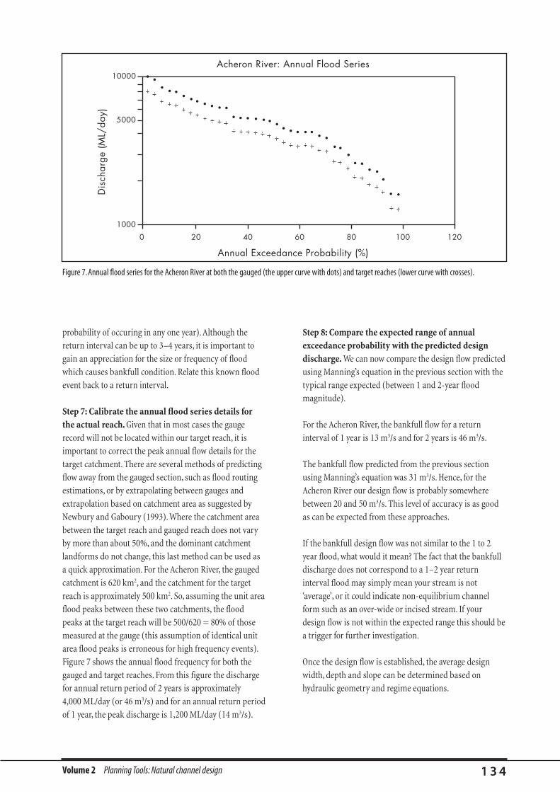
Volume 2 Planning Tools: Natural channel design 1 3 4
probability of occuring in any one year). Although the
return interval can be up to 3–4 years, it is important to
gain an appreciation for the size or frequency of flood
which causes bankfull condition. Relate this known flood
event back to a return interval.
Step 7: Calibrate the annual flood series details for
the actual reach. Given that in most cases the gauge
record will not be located within our target reach, it is
important to correct the peak annual flow details for the
target catchment. There are several methods of predicting
flow away from the gauged section, such as flood routing
estimations, or by extrapolating between gauges and
extrapolation based on catchment area as suggested by
Newbury and Gaboury (1993). Where the catchment area
between the target reach and gauged reach does not vary
by more than about 50%, and the dominant catchment
landforms do not change, this last method can be used as
a quick approximation. For the Acheron River, the gauged
catchment is 620 km2, and the catchment for the target
reach is approximately 500 km2. So, assuming the unit area
flood peaks between these two catchments, the flood
peaks at the target reach will be 500/620 = 80% of those
measured at the gauge (this assumption of identical unit
area flood peaks is erroneous for high frequency events).
Figure 7 shows the annual flood frequency for both the
gauged and target reaches. From this figure the discharge
for annual return period of 2 years is approximately
4,000 ML/day (or 46 m3/s) and for an annual return period
of 1 year, the peak discharge is 1,200 ML/day (14 m3/s).
Step 8: Compare the expected range of annual
exceedance probability with the predicted design
discharge. We can now compare the design flow predicted
using Manning’s equation in the previous section with the
typical range expected (between 1 and 2-year flood
magnitude).
For the Acheron River, the bankfull flow for a return
interval of 1 year is 13 m3/s and for 2 years is 46 m3/s.
The bankfull flow predicted from the previous section
using Manning’s equation was 31 m3/s. Hence, for the
Acheron River our design flow is probably somewhere
between 20 and 50 m3/s. This level of accuracy is as good
as can be expected from these approaches.
If the bankfull design flow was not similar to the 1 to 2
year flood, what would it mean? The fact that the bankfull
discharge does not correspond to a 1–2 year return
interval flood may simply mean your stream is not
‘average’, or it could indicate non-equilibrium channel
form such as an over-wide or incised stream. If your
design flow is not within the expected range this should be
a trigger for further investigation.
Once the design flow is established, the average design
width, depth and slope can be determined based on
hydraulic geometry and regime equations.
Annual Exceedance Probability (%)
Acheron River: Annual Flood Series
Dis
char
ge (M
L/da
y)
1000
5000
0
10000
20 40 60 80 100 120
Figure 7. Annual flood series for the Acheron River at both the gauged (the upper curve with dots) and target reaches (lower curve with crosses).

Volume 2 Planning Tools: Natural channel design 1 3 5
This section describes two related approaches to designing
channel dimensions: hydraulic geometry and regime
equations.
3.1. Using hydraulic geometry equations to designchannel dimensions
3.1.1. Simple hydraulic geometry
The downstream hydraulic geometry methodology was
pioneered by Leopold and Maddock (1953) from studies of
a large sample of rivers in the Great Plains and south-west
area of the United States. In this simple approach, the
dependent channel variables, width (w), mean depth (d),
mean velocity (v) and slope (S), are related by simple
power functions to an index of discharge (Q), usually
channel forming discharge. Leopold and Maddock (1953)
did not consider channel slope in their analysis.
w = aQb
d = cQf
S = kQm
The coefficients a, c, and k and the exponents b, f, and m
are empirically derived. Given a design discharge (ie.
bankfull as estimated above) one can predict the expected
size and shape of the channel.
Downstream changes in channel geometry can be
investigated by linking information from a number of sites
within a stream system (Gordon et al., 1992: p. 309).
Leopold and Maddock (1953) cited downstream
coefficients of b = 0.5 and f = 0.4.
Chong (1970: p.882) concluded that "…rivers in different
geologic, physiographic and climatic regions tend to
behave in much the same way…", but later, Park (1977)
who examined worldwide hydraulic geometry exponent
data from 72 streams from a variety of climates concluded
that there was a great deal of variation in the relationship
between channel morphology and discharge or catchment
area.
3.1.2. Some general guidelines for simple hydraulic geometry
(Note that the higher the exponent, then the faster the rate
of change downstream.)
• Streams in humid areas tend to have medium to high
width exponents (0.4–0.8) and medium depth
exponents (0.2–0.6).
• Tropical streams tend to display low to medium width
exponents (0.2–0.4), and low to medium depth
exponents (0.2–0.6).
• A distinction can be drawn between the hydraulic
geometries of perennial streams and ephemeral
streams in the semi-arid environment. Perennial
streams exhibit exponent values similar to that of
humid temperate streams, whereas ephemeral streams
tend to have low width exponents (<0.3).
• A single tidal estuary study by Langbein (1963) showed
different exponents to those of non-tidal streams.
Width exponent was high (0.6–0.8) and the depth
exponent was high (0.6–0.8).
• Huang and Nanson’s (1997) work on four streams in
the Illawarra region found that values of the exponents
b, f, and m varied considerably between streams and in
some cases even exceeded the full range of values
obtained internationally. When considering gravel bed
and sand bed streams separately, the exponents for
average depth (f) in sand channels were close to the
modes observed for worldwide data, while the
exponents for width (b) were extreme outliers.
• For the Acheron catchment in Victoria, Gordon used
channel maintenance flow for the development of
geometry relationships rather than the bankfull
discharge (which is higher) (Gordon, 1996). The
hydraulic exponents were found to be b = 0.48 and
f = 0.35, which are within the range of the worldwide
values.
• For the Hunter Valley, Gippel (1985) found that when
catchment area was used as the independent variable,
3. Hydraulic geometry equations and regime equations
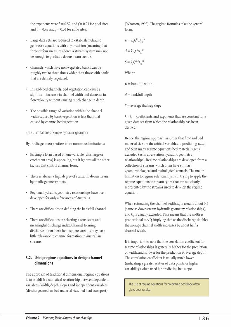
Volume 2 Planning Tools: Natural channel design 1 3 6
the exponents were b = 0.52, and f = 0.23 for pool sites
and b = 0.48 and f = 0.34 for riffle sites.
• Large data sets are required to establish hydraulic
geometry equations with any precision (meaning that
three or four measures down a stream system may not
be enough to predict a downstream trend).
• Channels which have non-vegetated banks can be
roughly two to three times wider than those with banks
that are densely vegetated.
• In sand-bed channels, bed vegetation can cause a
significant increase in channel width and decrease in
flow velocity without causing much change in depth.
• The possible range of variation within the channel
width caused by bank vegetation is less than that
caused by channel bed vegetation.
3.1.3 . Limitations of simple hydraulic geometry
Hydraulic geometry suffers from numerous limitations:
• Its simple form based on one variable (discharge or
catchment area) is appealing, but it ignores all the other
factors that control channel form.
• There is always a high degree of scatter in downstream
hydraulic geometry plots.
• Regional hydraulic geometry relationships have been
developed for only a few areas of Australia.
• There are difficulties in defining the bankfull channel.
• There are difficulties in selecting a consistent and
meaningful discharge index. Channel forming
discharge in northern hemisphere streams may have
little relevance to channel formation in Australian
streams.
3.2. Using regime equations to design channeldimensions
The approach of traditional dimensional regime equations
is to establish a statistical relationship between dependent
variables (width, depth, slope) and independent variables
(discharge, median bed material size, bed load transport)
(Wharton, 1992). The regime formulas take the general
form:
w = k1Qk2D
50k3
d = k4Qk5D
50
k6
S = k7Qk8D
50k9
Where:
w = bankfull width
d = bankfull depth
S = average thalweg slope
k1–k
9= coefficients and exponents that are constant for a
given data set from which the relationship has been
derived.
Hence, the regime approach assumes that flow and bed
material size are the critical variables to predicting w, d,
and S; in many regime equations bed material size is
excluded (as in at-a-station hydraulic geometry
relationships). Regime relationships are developed from a
collection of streams which often have similar
geomorphological and hydrological controls. The major
limitation to regime relationships is in trying to apply the
regime equations to stream types that are not clearly
represented by the streams used to develop the regime
equation.
When estimating the channel width, k2
is usually about 0.5
(same as downstream hydraulic geometry relationships),
and k3
is usually excluded. This means that the width is
proportional to ÃQ, implying that as the discharge doubles
the average channel width increases by about half a
channel width.
It is important to note that the correlation coefficient for
regime relationships is generally higher for the prediction
of width, and is lower for the prediction of average depth.
The correlation coefficient is usually much lower
(indicating a greater scatter of data points or higher
variability) when used for predicting bed slope.
The use of regime equations for predicting bed slope often
gives poor results.

Volume 2 Planning Tools: Natural channel design 1 3 7
3.2.1. Which equation should you use?
Research into regime relationships by Dr Graham Jenkins,
Neranjala Fernando and Robin Black at Queensland
University of Technology on two, small, ephemeral
Brisbane (rural) streams indicated that vegetation is a
significant control on stream geometry (Jenkins et al.,
1997). The streams investigated were Bullock Head Creek
(sand bed) and Moggill Creek (gravel bed, cohesive
banks). The coefficients developed by Hey and Thorne
(Table 20) were found to best represent the hydraulic
geometry of these streams.
Work by the Department of Land and Water Conservation
on northern coastal New South Wales rivers also indicated
that the Hey and Thorne coefficients were the most
applicable for gravel bed streams in that region.
The Brisbane City Council’s ‘Hydraulic Geometry of
Brisbane Streams: Guidelines for Natural Channel Design’
(Ian Drummond and Associates, 1996) recommends the
application of Hey and Thorne coefficients for gravel bed
streams, and Simons and Albertson coefficients for sand
bed streams (see Table 19).
Table 19. Recommended regime equations for south-eastern
Queensland streams (from Conrick and Ribi, 1996).
Bed Banks Recommended regime
relationship
Coarse (gravel) Coarse (gravel) Hey and Thorne (1986)
Coarse (gravel) Cohesive Hey and Thorne (1986)
Sand Sand Simons and Albertson (1963)
Sand Cohesive Simons and Albertson (1963)
Cohesive Cohesive Simons and Albertson (1963)
Non-cohesive material
For non-cohesive material (ie. no clay content) the
channel-forming process is thought to be related to erosive
forces, which are in turn related to boundary shear-stress
and particle size. Hence, a regime channel is one that is
more or less balanced between erosion and deposition
during bankfull flows. Regime relationships developed
from a data set of streams with non-cohesive beds and
banks tend to give reasonable correlation. This may be
because of the relatively straightforward physical
processes of erosion in non-cohesive materials.
Cohesive material
Stream forms in cohesive material are not so easy to
predict, possibly because of the complex chemical
processes which give clay its cohesive properties. There is
an extensive literature which looks at the erosive
properties of cohesive material (Enger et al., 1968;
Partheniades, 1971; Mehta et al., 1989a; Mehta et al.,
1989b). However, the complex properties of cohesive
material make analysis of the erosion process much more
difficult than for non-cohesive material. A paper by
Brekhovskikh et al. (1991) shows that erosion of cohesive
sediment could even be influenced by the presence of
benthic organisms.
Simons and Albertson (1963) worked on US and Indian
canals. They differentiated between bed and bank
materials, and as such the regime relationships they
developed in 1963 are still some of the best we have for
cohesive bed and banks, and sand bed with cohesive bank
streams.
So which equations should you use?
The best approach for using regime relationships is to
develop your own equations from a locally derived
database. It obviously takes a fair bit of time and effort to
develop a reliable database, so the quick alternative is to
calibrate existing relationships with your stream. Collect
data (Q, w, d, S, vegetation type and density) from a series
of equilibrium cross-sections and compare the measured
data with the results you obtain using the equations in
Table 20. The physical conditions used to derive these
equations are described in Table 21.
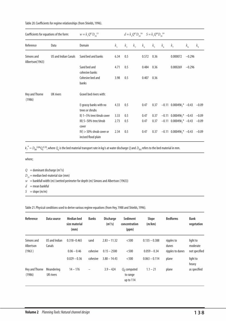
Volume 2 Planning Tools: Natural channel design 1 3 8
Table 21. Physical conditions used to derive various regime equations (from Hey, 1988 and Shields, 1996).
Reference Data source Median bed Banks Discharge Sediment Slope Bedforms Bank
size material (m3/s) concentration (m/km) vegetation
(mm) (ppm)
Simons and US and Indian 0.318–0.465 sand 2.83 – 11.32 <500 0.135 – 0.388 ripples to light to
Albertson Canals dunes moderate
(1963 ) 0.06 – 0.46 cohesive 0.15 – 2500 <500 0.059 – 0.34 ripples to dunes not specified
0.029 – 0.36 cohesive 3.88 – 14.43 <500 0.063 – 0.114 plane light to
heavy
Hey and Thorne Meandering 14 – 176 – 3.9 – 424 Qs computed 1.1 – 21 plane as specified
(1986) UK rivers to range
up to 114
Table 20. Coefficients for regime relationships (from Shields, 1996).
Coefficients for equations of the form: w = k1Qk2D
50k3 d = k
4Qk5D
50k6 S = k
7Qk8D
50k9
Reference Data Domain k1
k2
k3
k4
k5
k6
k7
k8
k9
Simons and US and Indian Canals Sand bed and banks 6.34 0.5 0.572 0.36 0.000072 –0.296
Albertson(1963)
Sand bed and 4.71 0.5 0.484 0.36 0.000269 –0.296
cohesive banks
Cohesive bed and 3.98 0.5 0.407 0.36
banks
Hey and Thorne UK rivers Gravel bed rivers with:
(1986)
I) grassy banks with no 4.33 0.5 0.47 0.37 –0.11 0.00049k7* –0.43 –0.09
trees or shrubs
II) 1–5% tree/shrub cover 3.33 0.5 0.47 0.37 –0.11 0.00049k7* –0.43 –0.09
III) 5–50% tree/shrub 2.73 0.5 0.47 0.37 –0.11 0.00049k7* –0.43 –0.09
cover
IV) > 50% shrub cover or 2.34 0.5 0.47 0.37 –0.11 0.00049k7* –0.43 –0.09
incised flood plain
k7* = D84
0.84Qs0.10, where Qs is the bed material transport rate in kg/s at water discharge Q and D84 refers to the bed material in mm.
where;
Q = dominant discharge (m3/s)
D50
= median bed-material size (mm)
w = bankfull width (m) (wetted perimeter for depth (m) Simons and Albertson (1963))
d = mean bankful
S = slope (m/m)

Volume 2 Planning Tools: Natural channel design 1 3 9
The redesign of channel geometry has particular
application to streams which have undergone dramatic
morphological changes through response to land-use
practices or due to direct human interference with the
stream form (channelisation or straightening). To redesign
a channel we need to consider both the channel geometry
(cross-section variables) and channel planform. This
section summarises the commonly adopted methods of
channel cross-section design and the following section
details the design of channel plan form.
4.1. Channel depth variation
To maintain hydraulic variability in redesigned channels,
the depth must vary downstream and across channel. Depth
irregularities will form naturally in the redesigned channel
if scour velocities are high enough, however for cohesive or
armoured channels it is advisable to incorporate depth
variation at the design stage (Brookes, 1989).
Pools naturally form at locations with the highest scour
velocities (bends). Apmann’s (1972) equation and Hey and
Thorne’s (1986) equation can be used to estimate this pool
depth (measured from bankfull height).
Apmann’s equation for depth at bend is:
db= d[(3.5W/r
0)/(1–(1–W/r
0)3.5)]
and Hey and Thorne's equation for gravel bed streams is:
db= 0.20Q0.36 D
50–0.56 D
840.35
where:
db= depth at bend or maximum depth (measured from
bankfull height)
d = average depth from regime equation
W = average width from regime equation
r0 = radius of curvature of outer bank (see Figure 4)
D50
= diameter of sieve which 50% of bed material passes
D84
= diameter of sieve which 84% of bed material passes
Here are some other geometry equations produced by Hey
and Thorne which are useful as guides in design.
• Riffle width (RW)(to approximate width at point of
inflection between bends) (not to be used for incised
streams)
RW = 1.034 W
• Riffle depth (Rd) (used to define minimum depth,
measured from top of bank) (not to be used for incised
streams)
Rd = 0.951d
• Riffle maximum depth (measured from top of bank)
Rd = 0.912 db
4.2. Designing channel planform/sinuosity
Where suitable reference sites exist, it is recommended
that the template approach be used to design meander
planform. Reinstatement of the pre-disturbance course
using the template method is a commonly adopted basis
for small stream rehabilitation design (Brookes, 1987). The
pre-disturbance course can often be determined through
historical research and by looking for old meander paths
on aerial photography.
Planform should be empirically designed only when the
historical channel position is unknown or impractical to
resume. Planform is inherently linked to slope, such that
meanders are established through a floodplain according
to the degradation and accretion of sediment. It is
impossible to design a stream planform that will be
immediately stable. Streams with re-constructed planform
will experience degradation and accretion before a stable
planform is reached.
There are two basic approaches to designing stream
planform:
1) slope first; or
2) alignment first.
4. Channel design details
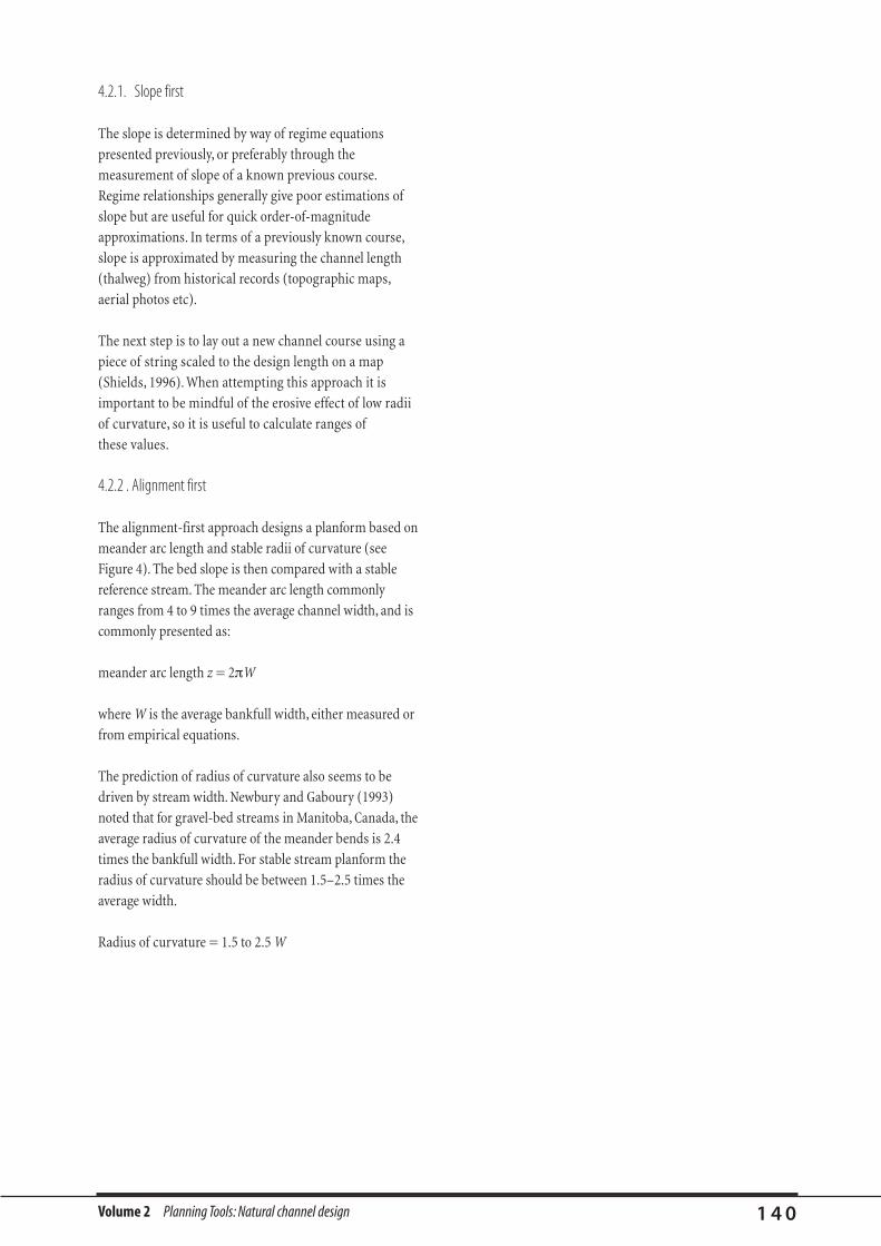
Volume 2 Planning Tools: Natural channel design 1 4 0
4.2.1. Slope first
The slope is determined by way of regime equations
presented previously, or preferably through the
measurement of slope of a known previous course.
Regime relationships generally give poor estimations of
slope but are useful for quick order-of-magnitude
approximations. In terms of a previously known course,
slope is approximated by measuring the channel length
(thalweg) from historical records (topographic maps,
aerial photos etc).
The next step is to lay out a new channel course using a
piece of string scaled to the design length on a map
(Shields, 1996). When attempting this approach it is
important to be mindful of the erosive effect of low radii
of curvature, so it is useful to calculate ranges of
these values.
4.2.2 . Alignment first
The alignment-first approach designs a planform based on
meander arc length and stable radii of curvature (see
Figure 4). The bed slope is then compared with a stable
reference stream. The meander arc length commonly
ranges from 4 to 9 times the average channel width, and is
commonly presented as:
meander arc length z = 2¹W
where W is the average bankfull width, either measured or
from empirical equations.
The prediction of radius of curvature also seems to be
driven by stream width. Newbury and Gaboury (1993)
noted that for gravel-bed streams in Manitoba, Canada, the
average radius of curvature of the meander bends is 2.4
times the bankfull width. For stable stream planform the
radius of curvature should be between 1.5–2.5 times the
average width.
Radius of curvature = 1.5 to 2.5 W

Albertson for sand bed streams) by referring to Table
20 and Table 21;
• use the design flow to predict channel geometry by
applying the regime equations; and
• design the planform and the pool depth variation for
the stream.
Volume 2 Planning Tools: Natural channel design 1 4 1
In this example we shall:
• collect relevant stream data; Q1.5
, vegetative cover, bed
material. D50, historical stream alignment;
• identify the regime equations which are suitable for
your stream type (slope, bed material etc; we use Hey
and Thorne for gravel bed streams and Simons and
5. A worked hypothetical application of the regime approach
Step 1: Stream details
A gravel bed stream has been realigned (due to road works) in
a straight course for 1,500 m leading and 500 m after a road
bridge.The stream is rapidly eroding; this is thought to be due
to increased velocity due to straightening.The relevant stream
characteristics are:
• gravel bed, D50
= 2 mm;
• from the unchannelised section on the stream the bankfull
discharge relates to approximately Q1.5
= 100 m3 /s;
• vegetation = minor shrub cover, some trees, say 20% of
bank has tree cover, the rest is grassed; and
• average bankfull width of unchannelised section ~ 25 m
(20–30 m).
Step 2: Select equation
Select Hey and Thorne equation: type III stream: 5–50%
tree/shrub cover.
Step 3: Predict channel geometry
w = 2.73Q0.5
Therefore, average stable width of the new channel should be
about w = 27 m (the width of the unchannelised reach is 25 m,
reasonably close to the predicted width).
d = 0.47Q0.37 2–0.11
Therefore, the average depth d = 2.4 m.
Step 4: Design planform
The old stream planform was determined by aerial
photographs and historical record.This planform is unsuitable
for the rehabilitated stream because of realignment for the
bridge and road. A new planform design is required. A bed
slope measured by comparing the thalweg to valley length
measured from a topographic map was 0.001 before
realignment, the current slope is 0.0022.
Meander arc length should be 2 ¹ 27
therefore average meander arc length = 170 m
Radius of curvature (r0)should be in the range:
r0
= 1.5 ´ 27 = 40 m
r0 = 2.5 ´ 27 = 67 m
Undertake iterative design to get acceptable slope
Target slope is 0.001,current slope is 0.0022 (distance = 2,000 m)
therefore drop = 4.4 m
for new slope, total channel length should be around = 4,400 m
The design approach is to lay out an approximate new stream
planform, then check the radius of curvature and meander
length to ensure the final shape is likely to be stable.
Step 5: Design pool depth variation
Design pool depth at each bend using Apmann’s equation
Pool depth = db= d[(3.5W/r
0)/(1–(1–W/r
0)3.5)]
Where r0
= 40 m, pool depth is 5.8 m.
Where r0
= 67 m, pool depth is 4.0 m.

Volume 2 Planning Tools: Natural channel design 1 4 2
The shortcomings of the empirical model approach are
that the hydraulic geometry and regime equations reflect
the data base from which they were derived (Hey and
Heritage, 1988). Hence, for hydraulic geometry equations
to be of use, the reference streams from which they were
derived must be similar to the target channel to be
rehabilitated.
The implication of this criticism of the regime approach in
Australia is that there has been limited confirmation of
specific regime equations for any stream types. Therefore,
regime equations should either be used cautiously on
Australian streams, or verification of hydraulic geometry
variables should be undertaken on similar streams of a
stable form.
Potential impacts associated with channel design depend
heavily on the site conditions before rehabilitation. For
example, in the case of a completely armoured (say
concrete) urban drainage channel which has been
redesigned, the concrete has been removed and the new
earth channel remeandered there are going to be at least
some short-term erosion and deposition problems until
the channel stabilises itself.
It is not possible to estimate the magnitude of the
secondary effects without considering each rehabilitation
project on a reach-by-reach basis, but in terms of
conservative designing, consider the following to be
potential impacts.
• Bank erosion.
• Development of knickpoints.
• Bed erosion.
• Loss of infrastructure such as bridges.
• Meander migration.
• Catastrophic widening.
6. Limitations of the empirical model approach

Volume 2 Planning Tools: Natural channel design 1 4 3
Streams are rarely stable over long time scales.
Geomorphologists now realise that channels are
continually adjusting their form in response to changes in
the processes that shape them. This is particularly the case
with streams that are subjected to periodic cycles of cut
and fill. While many streams incised following the phase of
major disturbance by Europeans, there is evidence that
this has happened many times before Europeans arrived.
Thus, we know that channels evolve, or go through distinct
cycles of incision, widening and migration, then
deposition, possibly followed by a new equilibrium form.
By correctly classifying the stage of this process that the
stream is in, it is possible to make predictions about
whether the channel is likely to enlarge in the near future,
or slowly contract. If it is in the phase of down-cutting or
widening, then it is a poor candidate for rehabilitation
because the works are likely to be destroyed.
As well as the traditional models of channel evolution
devised by Schumm (eg. Schumm, 1969), more ambitious
classification systems have been based on the evolution of
stream systems (eg. Rosgen, 1996). A catchment
characterisation system based on the evolution of channel
geomorphology has been developed at Macquarie
University (funded by LWRRDC) known as the River
Styles approach. The approach is detailed in a three-part
series titled Geomorphology and River Ecology in South-
eastern Australia: an Approach to Catchment
Characterisation (Brierley et al., 1996). The following
section summarises some aspects of the River Styles
approach.
1.1 The ‘River Styles’ classification scheme
Geomorphic units are the building blocks of river styles,
and explaining their character, distribution and
assemblage provides the key to the explanation of river
character and behaviour. So far the method has been
based mainly on observations of unregulated non-urban
New South Wales streams, but may have a much wider
application.
The context for the development of the river styles method
is that the traditional view of an equilibrium based river,
formed and maintained by some dominant discharge
condition may not apply to Australian streams. The
example of the disequilibrium provided in Brierley et al.
(1996) is the Bega River. Before European settlement,
stream morphology was based on chains-of-ponds and
swamps which had developed through a cut-and-fill
process involving multiple phases of incision spaced
thousands of years apart. Since European settlement, the
valley floors have gullied following vegetation clearing and
channel disturbance. The gullied streams will not return to
their pre-disturbance equilibrium condition, rather they
will stabilise over time to a new incised form. So, while a
bankfull or dominant discharge may be responsible for the
final shape of the modified streams, the evolutionary
process from chains-of-ponds to incised streams does not
conform to the traditional stream evolution process.
THE CHANNEL EVOLUTION APPROACH TOREHABILITATION DESIGN
This part of the manual links to Step 3 (How has your stream
changed) Step 4 (What are your stream’s main problems and
assets), Step 6 (What are you strategies) and Step 9 (How will
you design your project to achieve your objectives) in the
Stream rehabilitation procedure (Volume 1).
The concept of how streams evolve is very important for
stream rehabilitation.This is the basis for working out the
trajectories of assets and problems in Steps 3 and 4. An
understanding of how the stream will develop over time is
also vital for working out rehabilitation strategies (Step 6) and
designing the details of your rehabilitation (Step 9) so that
your final plan is working with the natural recovery of the
stream.
For descriptions of the evolutionary development of gullies,
incised streams, sand slugs etc. see the geomorphology
examples in the Common stream problems section of this
volume.
The channel evolution approach to rehabilitation design
places the current stream condition into a longer-term
geomorphological process perspective.This allows assessment
of natural recovery potential.

Volume 2 Planning Tools: Natural channel design 1 4 4
Within this context of synchronous incision of south-
eastern Australian streams, the key to stream
rehabilitation is to assess the stage of post-disturbance
evolution for each river, and determine the likely future
condition (Brierley et al., 1996).
The process of catchment characterisation in the river
styles methodology is based on a nested hierarchical
approach proposed by Frissell et al. (1986), which is
applied at three independent scales:
• Catchment scale
Review of catchment scale considerations such as
catchment size and shape, elevation, drainage patterns
and geology.
• Reach scale
Reach scale elements are based on sediment budgets,
ie. the reaches ability to store, accumulate and transfer
materials as well as their role as sediment source zones.
• Geomorphic unit scale
Geomorphic unit attributes are those features sculpted
from rock or depositional forms as rivers rework their
bed material. Instream habitat character is determined
largely by hydraulic interaction with these geomorphic
units such as in pool and riffle formation, the
development of bars and scour holes, sheets of sand in
a sediment slug, and meander cut-offs in lowland
reaches.
Brierley et al. (1996) suggested a five-stage approach to the
catchment characterisation procedure;
• Stage 1: Compile baseline data.
Relevant data are collected for each of the above three
scales.
• Stage 2: Data analysis.
The present river behaviour is explained on the basis of
the collected data in stage 1.
• Stage 3: Prediction of recovery potential.
Future river behaviour is predicted on the basis of
geomorphic process zone framework (ie. on the basis of
recent changes), sediment storage (ie. sediment balance
drives the stream forming process), and theoretical
river behaviour (use traditional notions of stream
evolution to predict future stream behaviour).
• Stage 4: Determine target condition; prioritisation of
catchment management issues.
On the basis of predicted behaviour in stage 3, river
management actions can be prioritised.
• Stage 5: Identification of suitable river structures.
Stream rehabilitation works can be designed on the
basis of the priorities from stage 4.
More details and applications of the River Styles approach
are provided in the following publications:
• Brierley, G. (1999). River Styles: an integrative
biophysical template for river management. In:
Rutherfurd, I.D. and Bartly, R. (eds) Proceedings of the
second Australian Stream Management Conference, pp.
93–100.
• Fryirs, K. (1999). The recovery potential of River Styles
in the Bega catchment, NSW: a catchment based
framework for prioritisation of river rehabilitation
strategies. In: Rutherfurd, I.D. and Bartly, R. (eds)
Proceedings of the second Australian Stream
Management Conference, pp. 279–286.
• Ferguson, R. (1999). Know your catchment! The
importance of understanding controls on river styles
and their distribution in catchment management. In:
Rutherfurd, I.D. and Bartly, R. (eds) Proceedings of the
second Australian Stream Management Conference, pp.
249–256.

Volume 2 Planning Tools: Natural channel design 1 4 5
Natural streams are untidy: they are full of woody debris,
have trees sticking into the stream, the banks are often
undercut, and the flow varies from local high velocity
zones over rocks and around logs, to still water conditions
in deep pools. The channel meanders across the
floodplain, varying in shape from a deep, narrow trench
where it is hard up against the floodplain wall to a broad,
shallow stretch between meander bends. Most human
impact on streams, such as channelisation, increasing
sediment loads, and removing snags and vegetation, has
reduced in-channel complexity, making them less messy
and more uniform. Much stream rehabilitation effort is
directed at making streams messy again by
reintroducing structures, vegetation or woody debris,
which creates habitat complexity and velocity
variation in the stream.
The habitat features detailed here are based on the
creation of hydraulic, depth, and substrate diversity in
response to an in-stream obstruction. The basic hydraulic
response to an in-channel obstruction is a scour hole
created at high flows which persists at low flows, creating
low-flow habitat.
PREDICTING THE SCOUR PRODUCED WHENYOU PUT THINGS INTO STREAMS
To achieve a high species richness in a rehabilitated reach,
there must be a complex in-stream habitat. One indicator
of complex habitat is a large range of flow velocities in the
reach at any one time. Consider a stream as a rectangular
channel; the average velocity is equal to the flow rate
divided by the cross-sectional area (V = Q/A). If we
constrain the channel by putting a groyne into the flow or
a full-width structure across the bottom of the channel,
the cross-sectional area decreases, so the average velocity
increases. The opposite is true if we expand the cross-
sectional area with large pools: then the average velocity
decreases. In general, for every increase in flow velocity at
one point there must be a corresponding decrease
elsewhere. If we look at velocity on a smaller scale, say
where rocks or logs are put into the channel, we see that
there is little effect on the overall velocity of the channel,
but that the velocity conditions around the obstruction
will range from much higher than the average velocity to
still water behind the object. Hydraulic diversity is also
increased by the scour hole and depositional bars that
form downstream of instream works. Fish and other
aquatic creatures (platypus, macroinvertebrates) are
dependent on complex velocity conditions for suitable
conditions for feeding, reproduction and resting.
If there is flow around an object the local turbulence will cause
scour.The scour creates hydraulic and depth variability, and the
bar formed downstream of the scour is usually coarser than
the normal bed material, creating substrate variability.
1. What happens when you put something into astream?
The purpose of this section of the manual is to help you to
predict where scour will occur if you put something into a
stream, and how much scour and deposition there is likely to
be.This is important, not only for predicting the effectiveness
of your proposed works, but also for predicting potential
undesirable consequences of the work (see Step 8: Are your
objectives feasible? of the Stream rehabilitation planning
procedure,Volume 1).This section describes the general
erosion and deposition effects of placing any object into a
stream. It then goes on to provide some methods for
predicting the approximate depth of scour that can be
expected.The final section considers the position of scour
around objects.
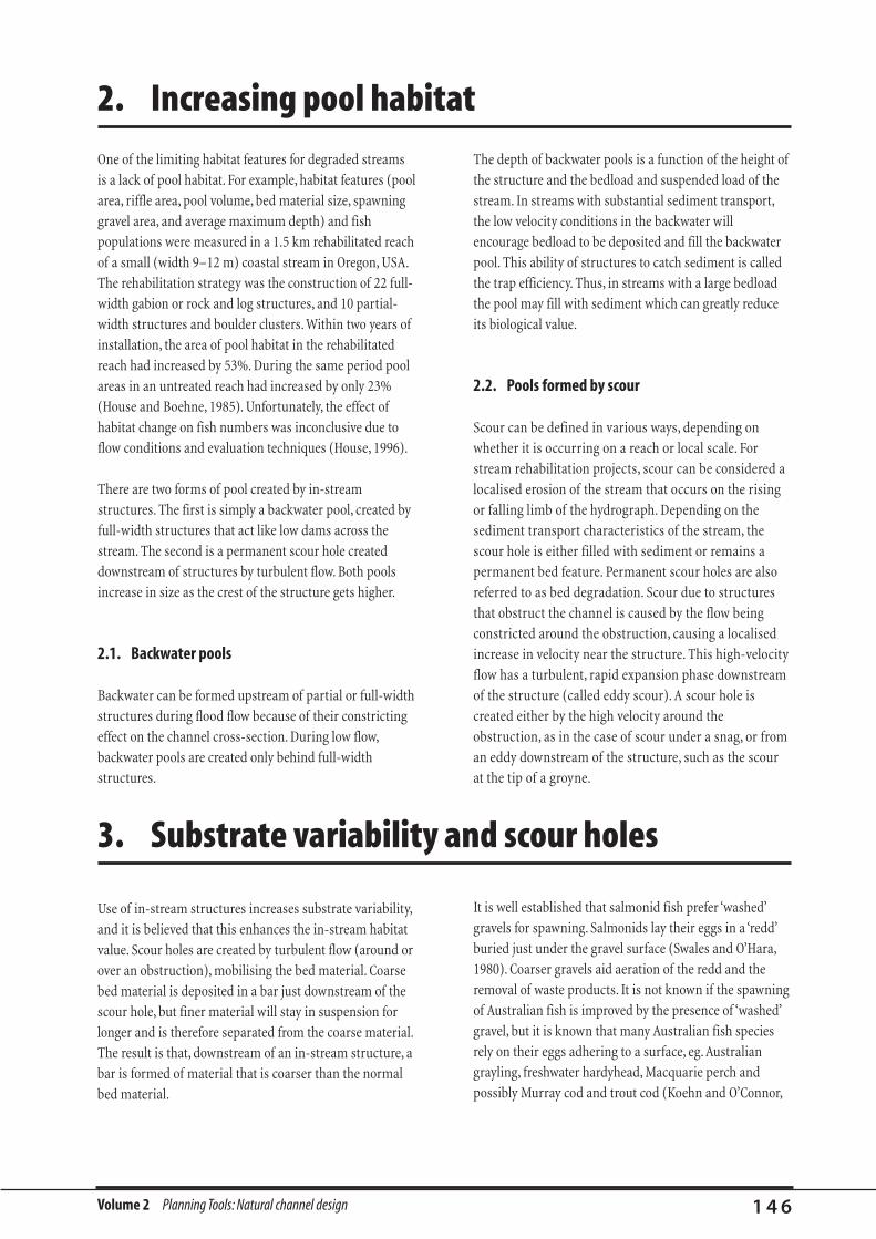
Volume 2 Planning Tools: Natural channel design 1 4 6
One of the limiting habitat features for degraded streams
is a lack of pool habitat. For example, habitat features (pool
area, riffle area, pool volume, bed material size, spawning
gravel area, and average maximum depth) and fish
populations were measured in a 1.5 km rehabilitated reach
of a small (width 9–12 m) coastal stream in Oregon, USA.
The rehabilitation strategy was the construction of 22 full-
width gabion or rock and log structures, and 10 partial-
width structures and boulder clusters. Within two years of
installation, the area of pool habitat in the rehabilitated
reach had increased by 53%. During the same period pool
areas in an untreated reach had increased by only 23%
(House and Boehne, 1985). Unfortunately, the effect of
habitat change on fish numbers was inconclusive due to
flow conditions and evaluation techniques (House, 1996).
There are two forms of pool created by in-stream
structures. The first is simply a backwater pool, created by
full-width structures that act like low dams across the
stream. The second is a permanent scour hole created
downstream of structures by turbulent flow. Both pools
increase in size as the crest of the structure gets higher.
2.1. Backwater pools
Backwater can be formed upstream of partial or full-width
structures during flood flow because of their constricting
effect on the channel cross-section. During low flow,
backwater pools are created only behind full-width
structures.
The depth of backwater pools is a function of the height of
the structure and the bedload and suspended load of the
stream. In streams with substantial sediment transport,
the low velocity conditions in the backwater will
encourage bedload to be deposited and fill the backwater
pool. This ability of structures to catch sediment is called
the trap efficiency. Thus, in streams with a large bedload
the pool may fill with sediment which can greatly reduce
its biological value.
2.2. Pools formed by scour
Scour can be defined in various ways, depending on
whether it is occurring on a reach or local scale. For
stream rehabilitation projects, scour can be considered a
localised erosion of the stream that occurs on the rising
or falling limb of the hydrograph. Depending on the
sediment transport characteristics of the stream, the
scour hole is either filled with sediment or remains a
permanent bed feature. Permanent scour holes are also
referred to as bed degradation. Scour due to structures
that obstruct the channel is caused by the flow being
constricted around the obstruction, causing a localised
increase in velocity near the structure. This high-velocity
flow has a turbulent, rapid expansion phase downstream
of the structure (called eddy scour). A scour hole is
created either by the high velocity around the
obstruction, as in the case of scour under a snag, or from
an eddy downstream of the structure, such as the scour
at the tip of a groyne.
2. Increasing pool habitat
3. Substrate variability and scour holes
Use of in-stream structures increases substrate variability,
and it is believed that this enhances the in-stream habitat
value. Scour holes are created by turbulent flow (around or
over an obstruction), mobilising the bed material. Coarse
bed material is deposited in a bar just downstream of the
scour hole, but finer material will stay in suspension for
longer and is therefore separated from the coarse material.
The result is that, downstream of an in-stream structure, a
bar is formed of material that is coarser than the normal
bed material.
It is well established that salmonid fish prefer ‘washed’
gravels for spawning. Salmonids lay their eggs in a ‘redd’
buried just under the gravel surface (Swales and O’Hara,
1980). Coarser gravels aid aeration of the redd and the
removal of waste products. It is not known if the spawning
of Australian fish is improved by the presence of ‘washed’
gravel, but it is known that many Australian fish species
rely on their eggs adhering to a surface, eg. Australian
grayling, freshwater hardyhead, Macquarie perch and
possibly Murray cod and trout cod (Koehn and O’Connor,
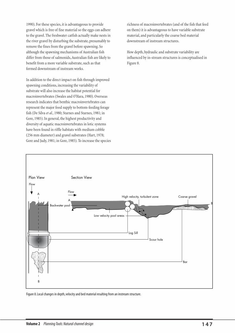
Volume 2 Planning Tools: Natural channel design 1 4 7
1990). For these species, it is advantageous to provide
gravel which is free of fine material so the eggs can adhere
to the gravel. The freshwater catfish actually make nests in
the river gravel by disturbing the substrate, presumably to
remove the fines from the gravel before spawning. So
although the spawning mechanisms of Australian fish
differ from those of salmonids, Australian fish are likely to
benefit from a more variable substrate, such as that
formed downstream of instream works.
In addition to the direct impact on fish through improved
spawning conditions, increasing the variability of
substrate will also increase the habitat potential for
macroinvertebrates (Swales and O’Hara, 1980). Overseas
research indicates that benthic macroinvertebrates can
represent the major food supply to bottom-feeding forage
fish (De Silva et al., 1980; Starnes and Starnes, 1981; in
Gore, 1985). In general, the highest productivity and
diversity of aquatic macroinvertebrates in lotic systems
have been found in riffle habitats with medium cobble
(256 mm diameter) and gravel substrates (Hart, 1978;
Gore and Judy, 1981; in Gore, 1985). To increase the species
richness of macroinvertebrates (and of the fish that feed
on them) it is advantageous to have variable substrate
material, and particularly the coarse bed material
downstream of instream structures.
How depth, hydraulic and substrate variability are
influenced by in-stream structures is conceptualised in
Figure 8.
����@@@@����ÀÀÀÀ����@@@@����ÀÀÀÀ
Plan View Section View
Scour hole
Flow
FlowA
A
B
B���@@@���ÀÀÀ���@@@���ÀÀÀLog Sill
Low velocity pool areas
Backwater pool
High velocity, turbulent zone Coarse gravel
Bar
Figure 8. Local changes in depth, velocity and bed material resulting from an instream structure.

Volume 2 Planning Tools: Natural channel design 1 4 8
4.1. Predicting the size of scour holes
For stream rehabilitation, it would be very useful to be able
to predict the size and location of scour holes so that we
know if structures will be threatened, or by how much
pool area will be increased. Unfortunately, we are unable to
do this with any great confidence. There is a general lack of
agreement between investigators as to which factors are
most important in determining scour depths (Copeland,
1983) although there is general agreement that the greatest
amount of scour occurs under clear-water scour
conditions (Richardson and Richardson, 1993; Yasi, 1997).
A wide range of models has been produced for predicting
the scour pattern around groynes.
A simple technique for estimating the scour downstream of
in-stream structures or disturbances like bridge piers,
groynes, and abutments is the Farraday and Charlton (1983)
method detailed below. For structures such as large woody
debris or boulders that are likely to be submerged, the scour
will be less than that predicted by this method. This method
is included to provide guidance on how much protection that
may need to be provided for structures placed in streams.
4.1.1. The Farraday and Charlton method
The basic equations used in this method are given below:
y2= 0.38(V1y
1)0.67D
50–0.17 (for sand bed channels)
y2= 0.47(V1y
1)0.8D
90–0.12 (for gravel bed channels)
y2
= 51.4n0.86(V1y
1)0.86T
c–0.43 (for cohesive bed channels)
where:
y2= mean depth of the total scour measured from the
water surface (m);
y1= design depth equal to A1/T
1(m) (usually adopted as
bankfull depth);
V1
= design flow velocity (m/s) (either measured or
estimated using Manning’s equation—see Selecting a
design discharge, in Natural channel design, this volume);
D50
= size of bed material such that 50% of the material is
smaller by mass (sieve sampling or field sampling for
coarse beds);
D90
= size of bed material such that 90% of the material is
smaller by mass (sieve sampling or field sampling for
coarse beds);
n = Manning’s roughness coefficient (see Selecting a design
discharge, in Natural channel design, for a method to
calculate Mannings n);
Tc= critical tractive stress for scour to occur for given bulk
density and soil type (read from Table 22);
T1
= mean top width for the design flow (m) (usually
taken as bankfull width); and
A1
= mean bankfull flow area for the design flow (m)
(usually taken as bankfull cross-sectional area).
Table 22. Critical tractive stress for cohesive bed material. (First select
the column based on the voids ratio and bulk density; second, select
N/m2 for that column given the soil type.)
Voids ratio 2.0–1.2 1.2–0.6 0.6–0.3 0.3–0.2
Dry bulk 880–1,220 1,200–1,650 1,650–2,030 2,030–2,210
density
(kg/m3)
Saturated 1,550–1,740 1,740–2,030 2,030–2,270 2,270–2,370
bulk density
(kg/m3)
Soil type Critical tractive stress (N/m2)
Sandy clay 1.9 7.5 15.7 30.2
Heavy clay 1.5 6.7 14.6 27.0
Clay 1.2 5.9 13.5 25.4
Loam clay 1.0 4.6 10.2 16.8
4. General hydraulic effects of instream structures
Note: Placing objects in streams can produce dramatic and
unwelcome erosion and deposition. For example, agencies
have incurred legal trouble for revegetation that constricted
flow and caused bank erosion. It is always wise to seek
professional advice.These notes provide only a general guide.
We recommend seeking professional advice in any project
where scour could cause a problem.
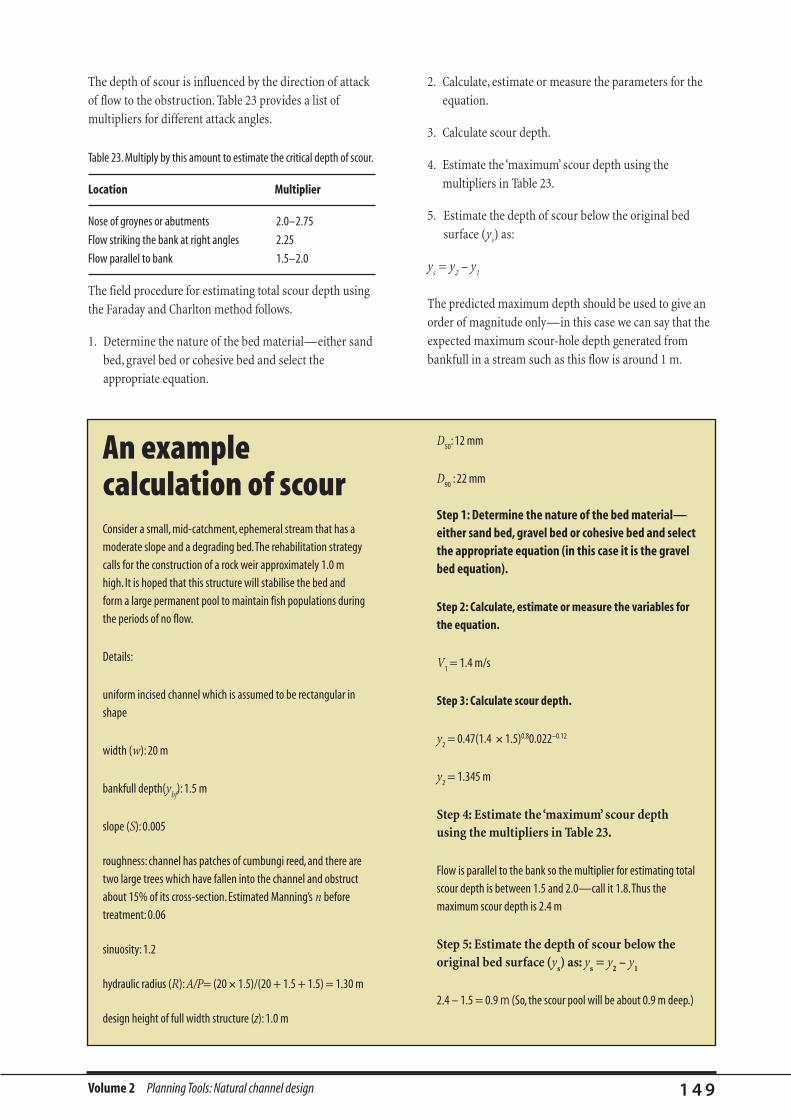
Volume 2 Planning Tools: Natural channel design 1 4 9
The depth of scour is influenced by the direction of attack
of flow to the obstruction. Table 23 provides a list of
multipliers for different attack angles.
Table 23.Multiply by this amount to estimate the critical depth of scour.
Location Multiplier
Nose of groynes or abutments 2.0–2.75
Flow striking the bank at right angles 2.25
Flow parallel to bank 1.5–2.0
The field procedure for estimating total scour depth using
the Faraday and Charlton method follows.
1. Determine the nature of the bed material—either sand
bed, gravel bed or cohesive bed and select the
appropriate equation.
2. Calculate, estimate or measure the parameters for the
equation.
3. Calculate scour depth.
4. Estimate the ‘maximum’ scour depth using the
multipliers in Table 23.
5. Estimate the depth of scour below the original bed
surface (ys) as:
ys= y
2– y
1
The predicted maximum depth should be used to give an
order of magnitude only—in this case we can say that the
expected maximum scour-hole depth generated from
bankfull in a stream such as this flow is around 1 m.
An examplecalculation of scourConsider a small, mid-catchment, ephemeral stream that has a
moderate slope and a degrading bed.The rehabilitation strategy
calls for the construction of a rock weir approximately 1.0 m
high. It is hoped that this structure will stabilise the bed and
form a large permanent pool to maintain fish populations during
the periods of no flow.
Details:
uniform incised channel which is assumed to be rectangular in
shape
width (w): 20 m
bankfull depth(ybf
): 1.5 m
slope (S): 0.005
roughness: channel has patches of cumbungi reed, and there are
two large trees which have fallen into the channel and obstruct
about 15% of its cross-section. Estimated Manning’s n before
treatment: 0.06
sinuosity: 1.2
hydraulic radius (R):A/P= (20 ´ 1.5)/(20 + 1.5 + 1.5) = 1.30 m
design height of full width structure (z): 1.0 m
D50
: 12 mm
D90
: 22 mm
Step 1: Determine the nature of the bed material—either sand bed, gravel bed or cohesive bed and selectthe appropriate equation (in this case it is the gravelbed equation).
Step 2: Calculate, estimate or measure the variables forthe equation.
V1
= 1.4 m/s
Step 3: Calculate scour depth.
y2
= 0.47(1.4 ´ 1.5)0.80.022–0.12
y2
= 1.345 m
Step 4: Estimate the ‘maximum’ scour depth
using the multipliers in Table 23.
Flow is parallel to the bank so the multiplier for estimating total
scour depth is between 1.5 and 2.0—call it 1.8.Thus the
maximum scour depth is 2.4 m
Step 5: Estimate the depth of scour below the
original bed surface (ys) as: y
s= y
2– y
1
2.4 – 1.5 = 0.9 m (So, the scour pool will be about 0.9 m deep.)
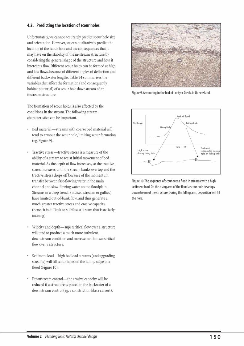
Volume 2 Planning Tools: Natural channel design 1 5 0
4.2. Predicting the location of scour holes
Unfortunately, we cannot accurately predict scour hole size
and orientation. However, we can qualitatively predict the
location of the scour hole and the consequences that it
may have on the stability of the in-stream structure by
considering the general shape of the structure and how it
intercepts flow. Different scour holes can be formed at high
and low flows, because of different angles of deflection and
different backwater lengths. Table 24 summarises the
variables that affect the formation (and consequently
habitat potential) of a scour hole downstream of an
instream structure.
The formation of scour holes is also affected by the
conditions in the stream. The following stream
characteristics can be important.
• Bed material—streams with coarse bed material will
tend to armour the scour hole, limiting scour formation
(eg. Figure 9).
• Tractive stress—tractive stress is a measure of the
ability of a stream to resist initial movement of bed
material. As the depth of flow increases, so the tractive
stress increases until the stream banks overtop and the
tractive stress drops off because of the momentum
transfer between fast-flowing water in the main
channel and slow-flowing water on the floodplain.
Streams in a deep trench (incised streams or gullies)
have limited out-of-bank flow, and thus generate a
much greater tractive stress and erosive capacity
(hence it is difficult to stabilise a stream that is actively
incising).
• Velocity and depth—supercritical flow over a structure
will tend to produce a much more turbulent
downstream condition and more scour than subcritical
flow over a structure.
• Sediment load—high bedload streams (and aggrading
streams) will fill scour holes on the falling stage of a
flood (Figure 10).
• Downstream control—the erosive capacity will be
reduced if a structure is placed in the backwater of a
downstream control (eg. a constriction like a culvert).
Figure 9. Armouring in the bed of Lockyer Creek, in Queensland.
Discharge
Time
Rising limb
Falling limb
Peak of flood
High scour during rising limb
Sediment redeposited in scour hole on falling limb
Figure 10.The sequence of scour over a flood in streams with a high
sediment load. On the rising arm of the flood a scour hole develops
downstream of the structure. During the falling arm, deposition will fill
the hole.
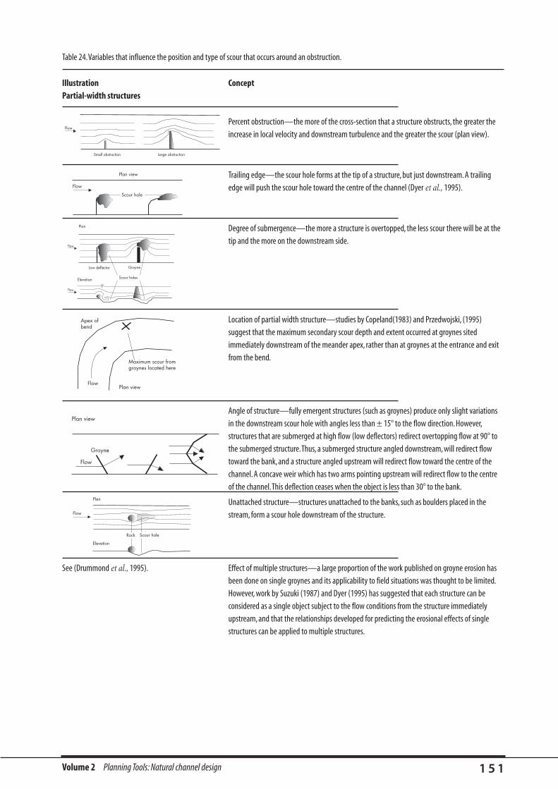
Volume 2 Planning Tools: Natural channel design 1 5 1
Table 24.Variables that influence the position and type of scour that occurs around an obstruction.
Illustration ConceptPartial-width structures
[figure PtaT241] Percent obstruction—the more of the cross-section that a structure obstructs, the greater the
increase in local velocity and downstream turbulence and the greater the scour (plan view).
[figure PtaT242] Trailing edge—the scour hole forms at the tip of a structure, but just downstream. A trailing
edge will push the scour hole toward the centre of the channel (Dyer et al., 1995).
[figure PtaT243] Degree of submergence—the more a structure is overtopped, the less scour there will be at the
tip and the more on the downstream side.
[figure PtaT244] Location of partial width structure—studies by Copeland(1983) and Przedwojski, (1995)
suggest that the maximum secondary scour depth and extent occurred at groynes sited
immediately downstream of the meander apex, rather than at groynes at the entrance and exit
from the bend.
[figure PtaT245] Angle of structure—fully emergent structures (such as groynes) produce only slight variations
in the downstream scour hole with angles less than ± 15° to the flow direction. However,
structures that are submerged at high flow (low deflectors) redirect overtopping flow at 90° to
the submerged structure.Thus, a submerged structure angled downstream, will redirect flow
toward the bank, and a structure angled upstream will redirect flow toward the centre of the
channel. A concave weir which has two arms pointing upstream will redirect flow to the centre
of the channel.This deflection ceases when the object is less than 30° to the bank.
[figure PtaT246] Unattached structure—structures unattached to the banks, such as boulders placed in the
stream, form a scour hole downstream of the structure.
See (Drummond et al., 1995). Effect of multiple structures—a large proportion of the work published on groyne erosion has
been done on single groynes and its applicability to field situations was thought to be limited.
However, work by Suzuki (1987) and Dyer (1995) has suggested that each structure can be
considered as a single object subject to the flow conditions from the structure immediately
upstream, and that the relationships developed for predicting the erosional effects of single
structures can be applied to multiple structures.
Small obstruction Large obstruction
Flow
Scour hole
Flow
Plan view
Scour holes
GroyneLow deflector
Plan
Elevation
Flow
Flow
Maximum scour from groynes located here
Flow
Apex of bend
Plan view
Plan view
Flow
Groyne
Rock Scour hole
Elevation
Plan
Flow

Volume 2 Planning Tools: Natural channel design 1 5 2
Illustration ConceptFull-width structures
Eddy scour—scalloping of the bank downstream of a full-width structure is common.This
usually extends about one channel width downstream of the structure and is caused by
turbulent flow expansion as the water passes over the structure.
Downstream face angle—a gently sloping downstream face (eg. rock chutes) will generally not
produce a scour hole because energy is dissipated on the face of the structure and not on the
downstream bed.This contrasts with structures such as log sills that have a steep downstream
angle, and often considerable scour.
[figure PtaT2410] Height—higher structures will create a larger backwater, and the increased height will lead to a
larger downstream scourhole (Breusers and Raudkivi, 1991)
[figure PtaT2411] Trap efficiency—the lower velocity conditions of the backwater behind full-width structures
allows deposition of suspended sediment. If a reach is treated with a series of full-width
structures, the cumulative sediment trapping action can starve downstream reaches of
sediment, resulting in clearwater scour. However, in streams with high sediment loads, the
backwaters are likely to fill with sediment and subsequent bedload will pass over the full-width
structures.
[figure PtaT2412] Complex structures—Complex structures such as large woody debris (LWD) can span a
section, or all of the channel.They are sometimes fully attached to the bed, but usually
fall into the channel on an angle, allowing flow both over and under the snag. LWD also has
a complex array of branches that protrude into the flow and often catch other debris.The net
effect of LWD in the stream is much like the addition of a combination of complex engineered
structures.There is often scour under, downstream, and at both ends of LWD.
Scour hole Scour hole
Elevation
Plan
Flow
Flow
Scour hole
BackwaterBackwater
Low structureHigh structure
Plan
Elevation
Bar formation Scour hole
Flow
Bar formation����@@@@����ÀÀÀÀ����@@@@����ÀÀÀÀ
����@@@@����ÀÀÀÀ����@@@@����ÀÀÀÀ
Sediment starved stream
Sediment laden stream
Plan
Elevation
Plan
Elevation
Backwater pool
Backwater pool full of sediment
Shallow downstreampool
Deep downstream pool Downstream bar
Downstream bar
Flow
Flow
����@@@@����ÀÀÀÀ����@@@@����ÀÀÀÀ
������@@@@@@������ÀÀÀÀÀÀ������@@@@@@������ÀÀÀÀÀÀ
������@@@@@@������ÀÀÀÀÀÀ������@@@@@@������ÀÀÀÀÀÀ
Elevation
Plan
Flow
������@@@@@@������ÀÀÀÀÀÀ������@@@@@@������ÀÀÀÀÀÀ
Approx onechannel width
Bar formation
Scour
Plan view
Full width structure
Flow
Table 24 (cont’d).Variables that influence the position and type of scour that occurs around an obstruction.

reservoir. The water velocity at the dam wall (known as the
control point) will be zero. As you travel upstream of the
wall, the water velocity gradually increases until the river
is flowing at its normal velocity, unaffected by the dam.
The distance from the dam wall upstream to where the
flow is unaffected by the dam is the backwater. Backwaters
are produced by every structure in a channel, not just
dams. The upstream extent of the backwater depends on
how much the water level is raised at the control point.
With a dam, you know the effect on water level. The
problem comes when trying to predict the rise in water
surface from some in-channel structure like a piece of
large woody debris. We will use the subsequent hydraulic
tools to roughly predict the increase in water level from
any obstruction in the channel.
As a stream manager needing to predict the hydraulic
effect of instream work you must understand the concepts
of backwaters, flow conditions, the energy equation and
Manning’s equation. The following section is a summary
of these open-channel flow concepts. Their application to
predicting hydraulic effects will become clear as we work
through some examples of stream rehabilitation projects
in the following section.
1.1. What is a backwater?
An integral concept of flooding is the notion of a
backwater. If you increase the water level upstream of
stream works you have created a ‘backwater’. A backwater
is the difference between the upstream water level with the
structure and the water level without it (Neill, 1973). Any
structure or roughness that creates a backwater is known
as a control point (because it controls upstream water
depth).
Backwaters are important because they control flooding.
Imagine that we have built a dam across a river, and you
are in a boat, measuring the velocity of the water in the
Volume 2 Planning Tools: Natural channel design 1 5 3
If you put snags back into a stream, build benches that
constrict a channel, or revegetate the channel, what effect
will this have on flood height and flood duration?
Conversely, will removing those willows in the stream
dramatically reduce flooding? These are fundamental
questions for stream rehabilitators. This section, with
worked examples, provides some guidance on the effects
that doing things in streams has on flood levels.
To assess the likely effect of in-stream work on flooding we
need first to understand some basic open-channel
hydraulics so that we can tell if flow is subcritical, calculate
the critical depth for a given discharge and predict
roughness coefficients so that we can estimate the
discharge.
HOW CHANGING THE CHANNEL CANAFFECT FLOODING
1. Open-channel flow: general concepts and useful formulae
Note. Predicting hydraulic effects is a complex task. Here we
provide general information so that you can understand the
possible effects of your actions in the stream. It is essential to
get professional assistance if changing flood levels are likely to
lead to damage.
At the end of this section you will be able to roughly estimate
how changing things in a stream will affect how high floods
get, and how long they stay high.
Note. Many people believe that backwaters are created only
by dams that span the channel. In reality, anything that resists
flow produces a backwater during subcritical flows.Examples
are channel constrictions, logs, bushes, rock chutes, culverts a
wide shallow reach etc.All these features can ‘back the water
up’.
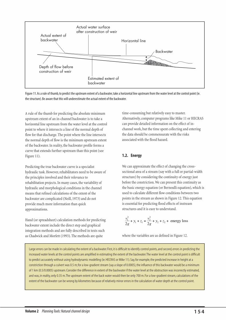
Volume 2 Planning Tools: Natural channel design 1 5 4
A rule of the thumb for predicting the absolute minimum
upstream extent of an in-channel backwater is to take a
horizontal line upstream from the water level at the control
point to where it intersects a line of the normal depth of
flow for that discharge. The point where the line intersects
the normal depth of flow is the minimum upstream extent
of the backwater. In reality, the backwater profile forms a
curve that extends further upstream than this point (see
Figure 11).
Predicting the true backwater curve is a specialist
hydraulic task. However, rehabilitators need to be aware of
the principles involved and their relevance to
rehabilitation projects. In many cases, the variability of
hydraulic and morphological conditions in the channel
means that refined calculations of the extent of the
backwater are complicated (Neill, 1973) and do not
provide much more information than quick
approximations.
Hand (or spreadsheet) calculation methods for predicting
backwater extent include the direct step and graphical
integration methods and are fully described in texts such
as Chadwick and Morfett (1993). The methods are quite
time-consuming but relatively easy to master.
Alternatively, computer programs like Mike 11 or HECRAS
can provide detailed information on the effect of in-
channel work, but the time spent collecting and entering
the data should be commensurate with the risks
associated with the flood hazard.
1.2. Energy
We can approximate the effect of changing the cross-
sectional area of a stream (say with a full or partial-width
structure) by considering the continuity of energy just
before the constriction. We can present this continuity as
the basic energy equation (or Bernoulli equation), which is
used to calculate different flow conditions between two
points in the stream as shown in Figure 12. This equation
is essential for predicting flood effects of instream
structures and it is easy to understand.
where the variables are as defined in Figure 12.
v
gy z
v
gy z1
2
1 122
2 22 2+ + = + + + energy loss
Estimated extent of backwater
Actual extent of backwater
Backwater
Depth of flow before construction of weir
Horizontal line
Actual water surface after construction of weir
Figure 11. As a rule of thumb, to predict the upstream extent of a backwater, take a horizontal line upstream from the water level at the control point (ie.
the structure). Be aware that this will underestimate the actual extent of the backwater.
Large errors can be made in calculating the extent of a backwater. First, it is difficult to identify control points, and second, errors in predicting the
increased water levels at the control points are amplified in estimating the extent of the backwater.The water level at the control point is difficult
to predict accurately without using hydrodynamic modelling (ie. HECRAS or Mike 11). Say, for example, the predicted increase in height at a
constriction through a culvert was 0.5 m; for a low-gradient stream (say a slope of 0.0005), the influence of this backwater would be a minimum
of 1 km (0.5/0.0005) upstream. Consider the difference in extent of the backwater if the water level at the obstruction was incorrectly estimated,
and was, in reality, only 0.35 m.The upstream extent of the back water would then be only 700 m. For a low-gradient stream, calculations of the
extent of the backwater can be wrong by kilometres because of relatively minor errors in the calculation of water depth at the control point.
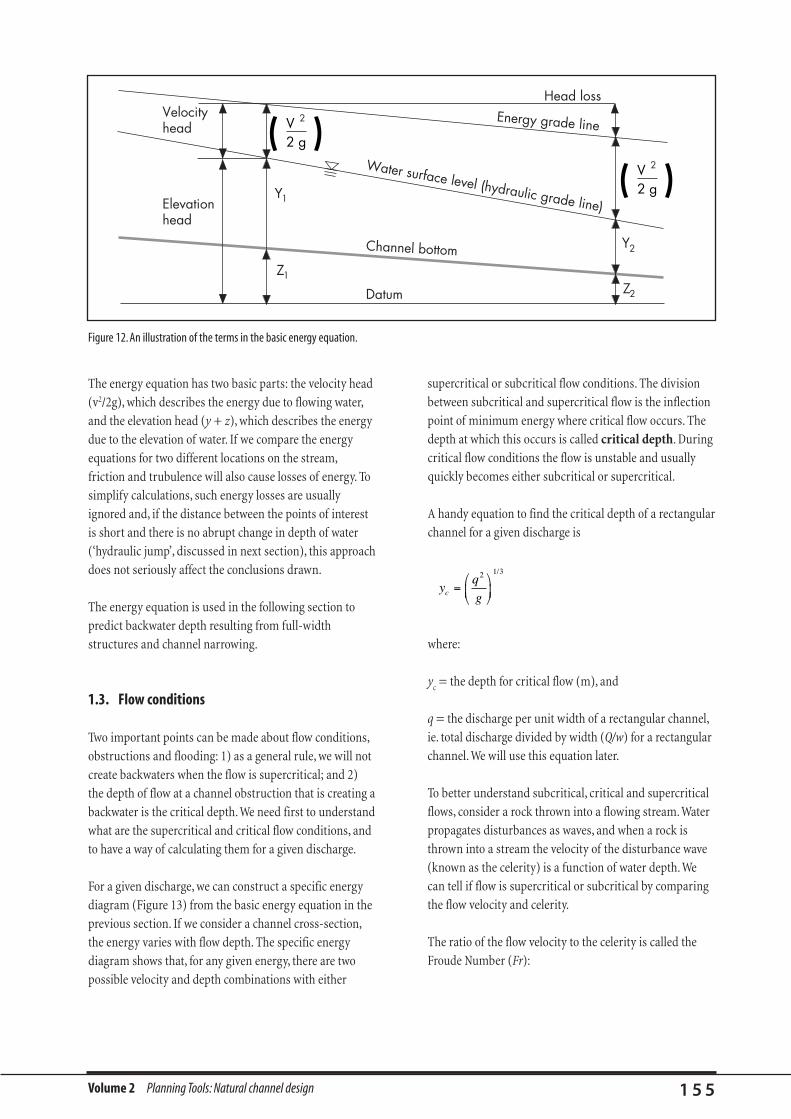
Volume 2 Planning Tools: Natural channel design 1 5 5
The energy equation has two basic parts: the velocity head
(v2/2g), which describes the energy due to flowing water,
and the elevation head (y + z), which describes the energy
due to the elevation of water. If we compare the energy
equations for two different locations on the stream,
friction and trubulence will also cause losses of energy. To
simplify calculations, such energy losses are usually
ignored and, if the distance between the points of interest
is short and there is no abrupt change in depth of water
(‘hydraulic jump’, discussed in next section), this approach
does not seriously affect the conclusions drawn.
The energy equation is used in the following section to
predict backwater depth resulting from full-width
structures and channel narrowing.
1.3. Flow conditions
Two important points can be made about flow conditions,
obstructions and flooding: 1) as a general rule, we will not
create backwaters when the flow is supercritical; and 2)
the depth of flow at a channel obstruction that is creating a
backwater is the critical depth. We need first to understand
what are the supercritical and critical flow conditions, and
to have a way of calculating them for a given discharge.
For a given discharge, we can construct a specific energy
diagram (Figure 13) from the basic energy equation in the
previous section. If we consider a channel cross-section,
the energy varies with flow depth. The specific energy
diagram shows that, for any given energy, there are two
possible velocity and depth combinations with either
supercritical or subcritical flow conditions. The division
between subcritical and supercritical flow is the inflection
point of minimum energy where critical flow occurs. The
depth at which this occurs is called critical depth. During
critical flow conditions the flow is unstable and usually
quickly becomes either subcritical or supercritical.
A handy equation to find the critical depth of a rectangular
channel for a given discharge is
where:
yc
= the depth for critical flow (m), and
q = the discharge per unit width of a rectangular channel,
ie. total discharge divided by width (Q/w) for a rectangular
channel. We will use this equation later.
To better understand subcritical, critical and supercritical
flows, consider a rock thrown into a flowing stream. Water
propagates disturbances as waves, and when a rock is
thrown into a stream the velocity of the disturbance wave
(known as the celerity) is a function of water depth. We
can tell if flow is supercritical or subcritical by comparing
the flow velocity and celerity.
The ratio of the flow velocity to the celerity is called the
Froude Number (Fr):
yq
gc =æ
èç
ö
ø÷
2 1 3/
Figure 12. An illustration of the terms in the basic energy equation.
Y1
Z1
Head loss
Y
2
2
Z2
Energy grade line
Water surface level (hydraulic grade line)
Channel bottom
Datum
Velocityhead
Elevationhead
V 2 g( )
2V 2 g( )

Volume 2 Planning Tools: Natural channel design 1 5 6
where
v = depth averaged flow velocity of the stream (m/s);
g = acceleration due to gravity (9.8 m/s2); and
y = flow depth (m).
The term Ãgy is the disturbance wave celerity.
Consider again the rock thrown into a flowing stream. The
velocity of the disturbance waves (celerity) relative to a
stationary observer on the bank will depend on the flow
velocity of the stream. If the flow velocity is greater than
the celerity (Fr > 1), then flow is said to be supercritical
and waves from the rock will not travel upstream. When
the flow velocity and the celerity are equal, a stationary
wave front will form at the disturbance and the flow
condition is described as critical (Fr = 1). If the flow
velocity is less than the celerity then the flow is subcritical
and the disturbance wave from our rock can travel
upstream (Fr < 1).
Critical flow occurs where the channel cross-section has
been reduced, such as at full width structures and channel
constrictions. It is the occurrence of critical flow that
controls the upstream water level and backs-up water. This
is because there is, for a given discharge, only one critical
flow depth (Figure 13). Since there is only one critical flow
depth for a given discharge, if we know the discharge it is
relatively easy to work out how high the backwater will be
(ie. somewhat more than critical flow depth). A subsequent
section on predicting backwater effects gives two worked
examples of backwater depths due to critical flow: one is
for flow over a weir, the other is for a channel constriction.
1.4. Using Manning’s equation to predict changesin discharge through increased roughness
Critical flow occurs when a backwater is created by a
channel obstruction such as a full or partial width
structure. In these cases, it is the local constriction in the
channel area that acts as the control point and produces a
backwater. If we reduce the channel capacity on a reach
scale rather than at a point, flow conditions are affected by
the cumulative influence of roughness and drag from the
boundary material and elements such as logs or boulders
in the channel. There is no one critical control point, but
rather the water level increases for a given discharge
because the channel capacity has been reduced by the
addition of roughness elements. This situation could arise
from revegetation of a channel, the reintroduction of
snags, or placing several small structures in a reach of
stream. In such cases, we use a uniform flow equation and
define the change in channel capacity from in-stream
works in terms of a changed channel ‘roughness’. The
method entails comparing the pre-rehabilitation channel
roughness with an estimated post-rehabilitation channel
roughness and either the change in channel capacity or the
change in water level for a given discharge.Various
Figure 13. A typical specific-energy curve, showing the relationship between flow type and water depth. For a given specific energy (eg. E1), there are two
possible combinations of depth and flow type.
Specific Energy
Water depth
Subcritical flow for E1
Supercritical flow for E1
Minimum energy
E1
Frv
gy=
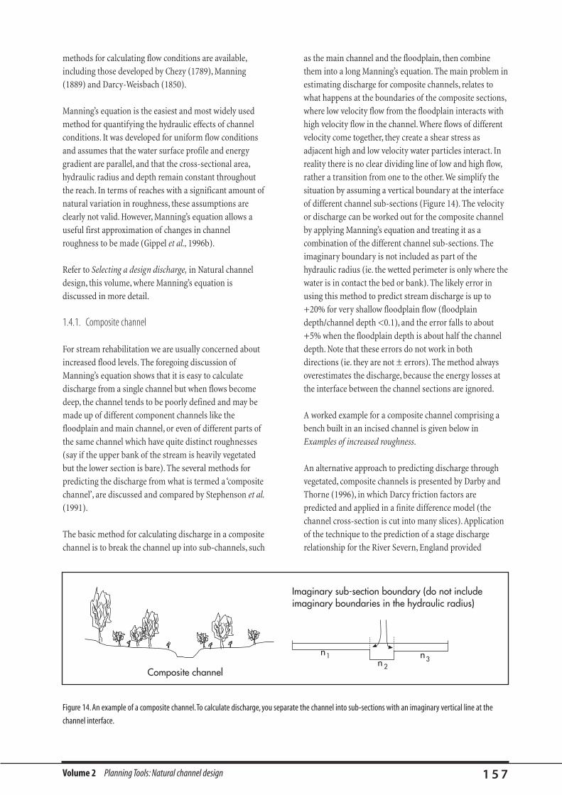
Volume 2 Planning Tools: Natural channel design 1 5 7
methods for calculating flow conditions are available,
including those developed by Chezy (1789), Manning
(1889) and Darcy-Weisbach (1850).
Manning’s equation is the easiest and most widely used
method for quantifying the hydraulic effects of channel
conditions. It was developed for uniform flow conditions
and assumes that the water surface profile and energy
gradient are parallel, and that the cross-sectional area,
hydraulic radius and depth remain constant throughout
the reach. In terms of reaches with a significant amount of
natural variation in roughness, these assumptions are
clearly not valid. However, Manning’s equation allows a
useful first approximation of changes in channel
roughness to be made (Gippel et al., 1996b).
Refer to Selecting a design discharge, in Natural channel
design, this volume, where Manning’s equation is
discussed in more detail.
1.4.1. Composite channel
For stream rehabilitation we are usually concerned about
increased flood levels. The foregoing discussion of
Manning’s equation shows that it is easy to calculate
discharge from a single channel but when flows become
deep, the channel tends to be poorly defined and may be
made up of different component channels like the
floodplain and main channel, or even of different parts of
the same channel which have quite distinct roughnesses
(say if the upper bank of the stream is heavily vegetated
but the lower section is bare). The several methods for
predicting the discharge from what is termed a ‘composite
channel’, are discussed and compared by Stephenson et al.
(1991).
The basic method for calculating discharge in a composite
channel is to break the channel up into sub-channels, such
as the main channel and the floodplain, then combine
them into a long Manning’s equation. The main problem in
estimating discharge for composite channels, relates to
what happens at the boundaries of the composite sections,
where low velocity flow from the floodplain interacts with
high velocity flow in the channel. Where flows of different
velocity come together, they create a shear stress as
adjacent high and low velocity water particles interact. In
reality there is no clear dividing line of low and high flow,
rather a transition from one to the other. We simplify the
situation by assuming a vertical boundary at the interface
of different channel sub-sections (Figure 14). The velocity
or discharge can be worked out for the composite channel
by applying Manning’s equation and treating it as a
combination of the different channel sub-sections. The
imaginary boundary is not included as part of the
hydraulic radius (ie. the wetted perimeter is only where the
water is in contact the bed or bank). The likely error in
using this method to predict stream discharge is up to
+20% for very shallow floodplain flow (floodplain
depth/channel depth <0.1), and the error falls to about
+5% when the floodplain depth is about half the channel
depth. Note that these errors do not work in both
directions (ie. they are not ± errors). The method always
overestimates the discharge, because the energy losses at
the interface between the channel sections are ignored.
A worked example for a composite channel comprising a
bench built in an incised channel is given below in
Examples of increased roughness.
An alternative approach to predicting discharge through
vegetated, composite channels is presented by Darby and
Thorne (1996), in which Darcy friction factors are
predicted and applied in a finite difference model (the
channel cross-section is cut into many slices). Application
of the technique to the prediction of a stage discharge
relationship for the River Severn, England provided
Figure 14. An example of a composite channel.To calculate discharge, you separate the channel into sub-sections with an imaginary vertical line at the
channel interface.
Composite channel
Imaginary sub-section boundary (do not include imaginary boundaries in the hydraulic radius)
n1n 2
n3
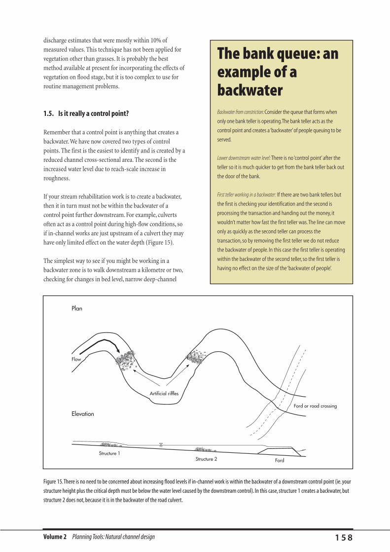
Volume 2 Planning Tools: Natural channel design 1 5 8
discharge estimates that were mostly within 10% of
measured values. This technique has not been applied for
vegetation other than grasses. It is probably the best
method available at present for incorporating the effects of
vegetation on flood stage, but it is too complex to use for
routine management problems.
1.5. Is it really a control point?
Remember that a control point is anything that creates a
backwater. We have now covered two types of control
points. The first is the easiest to identify and is created by a
reduced channel cross-sectional area. The second is the
increased water level due to reach-scale increase in
roughness.
If your stream rehabilitation work is to create a backwater,
then it in turn must not be within the backwater of a
control point further downstream. For example, culverts
often act as a control point during high-flow conditions, so
if in-channel works are just upstream of a culvert they may
have only limited effect on the water depth (Figure 15).
The simplest way to see if you might be working in a
backwater zone is to walk downstream a kilometre or two,
checking for changes in bed level, narrow deep-channel
Figure 15.There is no need to be concerned about increasing flood levels if in-channel work is within the backwater of a downstream control point (ie. your
structure height plus the critical depth must be below the water level caused by the downstream control). In this case, structure 1 creates a backwater, but
structure 2 does not, because it is in the backwater of the road culvert.
Structure 1Structure 2 Ford
Plan
ElevationFord or road crossing
Artificial riffles
Flow
The bank queue: anexample of abackwaterBackwater from constriction:Consider the queue that forms when
only one bank teller is operating.The bank teller acts as the
control point and creates a ‘backwater’of people queuing to be
served.
Lower downstream water level: There is no ‘control point’ after the
teller so it is much quicker to get from the bank teller back out
the door of the bank.
First teller working in a backwater: If there are two bank tellers but
the first is checking your identification and the second is
processing the transaction and handing out the money, it
wouldn’t matter how fast the first teller was.The line can move
only as quickly as the second teller can process the
transaction, so by removing the first teller we do not reduce
the backwater of people. In this case the first teller is operating
within the backwater of the second teller, so the first teller is
having no effect on the size of the ‘backwater of people’.

Volume 2 Planning Tools: Natural channel design 1 5 9
sections (ie. constrained channel), culverts, dense
vegetation, bridges, low-level crossings and other possible
control points.You should apply the methods in the
following sections to see if any of these potential controls
are creating a backwater in your reach. If you are working
in a backwater, you can assume that your rehabilitation
work will have no effect on flooding.
The water level downstream of an obstruction will be
lower, because once the stream has passed the control
point there is no restriction backing up the water (eg. just
downstream of structure 1 in Figure 15). This raises the
important point that if, during high flow, the water level
downstream of the suspected control point is not lower,
then either it is not really a control point, or further
downstream there must be some other control point, or a
combination of roughness elements, that is causing the
water to back up (eg. structure 2 in Figure 15).
2.1. Type of flooding
Now that we have covered the basic elements of open-
channel hydraulics, we can combine elements to predict
the effect of in-channel work on flooding.
First, we have to identify what ‘type’ of flooding we are
concerned about and what sort of in-channel modification
the stream rehabilitation project will use. We can then
provide various methods for predicting if flooding will be
affected and by how much.
It is important to define what we mean by a ‘flood’. When
river managers talk about ‘increased flooding’ they usually
mean one or other of the following:
• Increasing the maximum flood stage for an extreme
event (1 in 20 ARI flood or greater). For example, such
and such a treatment will increase flood levels so that
more of the town will be inundated by a 1 in 20-year
flood.
• Increased frequency of nuisance flooding (that is, the
channel capacity is reduced so that out-of-bank flows
occur twice instead of once a year).
• Increasing the duration of floods (ie. floods tend to stay
on the floodplain for longer).
2.1.1. Extreme event floods
Flooding occurs because the amount of water produced by
a storm is greater than the discharge capacity of the
stream. During large floods, the floodplain usually carries
most of the flow, and only a relatively small proportion of
the flood is carried in the main channel. For example,
5–15% of peak discharge (depending on where in the
catchment you look) of a 50-year flood on the Murray
River will be carried within the main channel, and the rest
on the floodplain. The proportion of flow in the channel is
likely to increase in smaller streams. Note that most
stream rehabilitation work is done in and around the
channel, so that since extreme event floods are dominated
by floodplain flow, the impact of stream rehabilitation on
major floods is not likely to be great.
An exception would be where the channel has been
reconstructed to carry extreme flows, eg. artificial
channels such as urban streams, or streams with full levee
protection. In these cases we can consider the whole
reconstructed channel as a compound low-flow and high-
flow channel (see example calculation of Artificial bench
formation, toward the end of the section).
Increased frequency of minor floods
Increased frequency of out-of-bank flows, or nuisance
flooding, is generally the type of flooding that farmers are
most concerned about, because it directly impedes access to
the floodplain and is considered to reduce the productivity
of floodplain farms. In this type of flooding most of the flow
remains in the main channel. These small floods can occur
several times in one year but are usually restricted to 1 to 5-
year events depending on the channel conditions.A clean,
straight channel has a greater flow capacity than a natural
meandering channel full of woody debris. Stream
rehabilitation work is usually undertaken in and around the
channel, so it is this type of flood that stream rehabilitation
work might affect. The examples in the following section
concentrate on flow that is just out-of bank.
2. Predicting backwater effects

Volume 2 Planning Tools: Natural channel design 1 6 0
Increased flood duration
Flood duration is a significant issue for both the
environment and farm protection; for example, a 2-day
inundation of a white clover crop will lead to a loss of more
than 6% of the annual yield (Maher, personal
communication). Equally, some flood persistence is
essential for the spawning of several fish species. The time
that a flood stays on the floodplain is a function of the
discharge capacity of the channel and floodplain, and of the
storm event that creates the flood. Predicting increased
flood levels for minor or extreme events is quite simple,
because it is a function of how much the flow exceeds the
discharge capacity of the channel and floodplain, but to
determin ‘how long’ flow is going to exceed capacity is a
more complicated story. To predict increases in flood
duration from stream rehabilitation projects we need to
conduct flood routing for different events before and after
the stream rehabilitation work. The flood routing must take
into account the changed channel and floodplain capacity.
The conclusion from the Wannon River example is that the
smaller capacity channel would have little effect on the
frequency of flooding, but a significant effect on flood
duration. However, it is unreasonable to compare out-of-
bank flow duration for different channel conditions
without considering the various types of storms that lead
to flooding.
To predict the effect of in-channel work on flood
duration you must route a series of flood events of
different sizes and types through the treated reach. To do
this, you must be familiar with a hydrological flood
routing model and have real flow records to compare the
effect of pre-and post-rehabilitation conditions on flood
duration. The prediction of changed flood duration is
not covered further in this manual. However, we do
emphasise that the duration of small floods can be
much more important for rehabilitators to consider
than the big floods that people usually worry about.
An example of flood duration for differentchannel capacities of the Wannon River,VictoriaThe flood duration for different channel capacities have been estimated for the Wannon River,Victoria (data provided by Peter Hill) as part of an
assessment of a proposal to remove large woody debris (LWD) from the channel (Sinclair Knight Merz, 1997).The effect of reducing or increasing
the channel capacity by 25% was investigated in terms of the number and duration of out-of-bank flows.The prediction was based on
hydrograph records from 1970 to 1995.The channel capacity is 5,300 m3/s and, during 1970–95 there were 29 out-of-bank flows. If we
increased the channel capacity by 25%, to 6,625 m3/s (say by removing all LWD and straightening the channel), then there would have been
only 24 out-of-bank flows during the period. If we reduced the channel capacity by 25%, to 3,975 m3/s (by adding LWD, or remeandering), then
the number of out-of-bank flows during the same period would have increased to 34.Therefore, for the period considered, a 25% increase or
decrease in the channel capacity resulted in an average change in flood frequency by one more (smaller channel) or one less (larger channel)
out-of-bank event every 4 years.This seems to be a small effect on flood frequency in comparison to the significant alterations required to
change the channel capacity by 25%.
However, if we look at the duration of out-of-bank flow for the three channel capacities, as shown on Figure 16, the out-of-bank flow obviously
lasted longer for the smaller channel. It is important to note the relative effectiveness of channel capacity change for different flood events.There
appears to be no direct relation between duration of out-of-bank flow and channel size. Consider event No. 21. For the 3,975 m3/s channel, flow
was out-of-bank for 16 days, while the same event in a 6,625 m3/s channel flow would resulted in out-of-bank flow for just 2 days.This event
probably had sustained high flow rather than a sharp peak, or a series of storms that maintained the discharge between 3,975 and 6,625 m3/s
for most of the event. For the small channel, almost all of the event was out of bank (only just) and for the large channel almost all of the event
was in-channel (only just). Compare this extreme result with a short, sharp storm shown by event 19, where for a channel capacity of 3,975 m3/s
the out-of-bank flow lasted for 14 days, only 2 days longer than for the 50% larger 6,625 m3/s channel. For this event, a fair proportion of the
flow was probably carried by the floodplains for both the small and large channels, So it is the combined channel and floodplain capacity, not
just the channel capacity, that influences the flood duration for this event.

Volume 2 Planning Tools: Natural channel design 1 6 1
Of the three types of flooding that we generally consider
(extreme events, increased frequency, and increased
duration), stream rehabilitation is most likely to affect
increased frequency and duration. The Wannon River
example has shown us that we can predict the increase in
flood frequency or duration by using historical flow data.
Flow data are usually not available, so the approach taken
in the following sections is to consider how stream
rehabilitation works affect the water level at bankfull
condition (that is, does it create a backwater?).
Alternatively, we can assess by how much the channel
capacity is modified by the work.
The following assessment of the potential increase in
water levels is divided into three types of channel
obstruction:
• full-width structures such as low weirs;
• partial-width obstructions such as groynes, retards and
channel narrowing; and
• general channel roughness such as in-channel
revegetation.
2.2. Flooding from full-width structures
The effect of a full-width structure is to reduce the channel
cross-sectional area. If the reduction in area is large
enough, the structure can control the water depth by
forming critical depth conditions over the structure. For a
given discharge the minimum depth of flow over a
structure will be the critical depth.
Full-width structures that are low compared with the flow
depth will be overtopped by a depth of water greater than
critical depth and will be ‘drowned out’; that is, they will
have no direct effect on the local surface water profile
other than that due to increased roughness (Figure 17A).
As the structure increases in height, it will reach a point
where the upstream water level is unchanged, but the
depth of flow over the structure is at critical depth (yc)
(Figure 17B). This is the point of maximum structure
height with no backwater increase. The depth of water over
the structure cannot be lower than critical depth, so if we
increase the height of the structure past this point, then
the upstream water depth must increase so that critical
depth is maintained over the structure (Figure 17C). Only
the conditions presented in Figure 17C will produce a
backwater from a full-width structure.
We can consider Figure 17C in terms of the energy
equation from section 1.2 Energy, above. Assuming no
energy loss, the energy at point (1) is the same as the
energy at point (2):
point (1) point (2)
Figure 16.The relationship between overbank flow duration and channel capacity, demonstrated by the flood record for the Wannon River.
Event no.
Q = 3975 ML/d
Q = 5300 ML/d
Q = 6625 ML/d
No.
of d
ays
of o
verb
ank
flow
1
5
0
10
15
20
25
30
35
40
45
50
3 5 7 9 11 13 15 17 19 21 23 25 27
yv
gy
v
gzc
c1
12 2
2 2+ = + + (1)
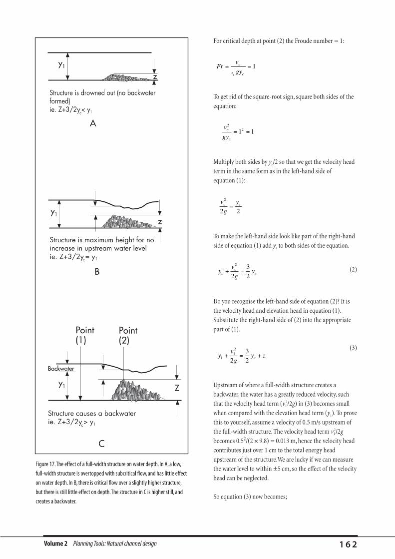
Volume 2 Planning Tools: Natural channel design 1 6 2
For critical depth at point (2) the Froude number = 1:
To get rid of the square-root sign, square both sides of the
equation:
Multiply both sides by yc/2 so that we get the velocity head
term in the same form as in the left-hand side of
equation (1):
To make the left-hand side look like part of the right-hand
side of equation (1) add yc to both sides of the equation.
(2)
Do you recognise the left-hand side of equation (2)? It is
the velocity head and elevation head in equation (1).
Substitute the right-hand side of (2) into the appropriate
part of (1).
(3)
Upstream of where a full-width structure creates a
backwater, the water has a greatly reduced velocity, such
that the velocity head term (v12/2g) in (3) becomes small
when compared with the elevation head term (y1). To prove
this to yourself, assume a velocity of 0.5 m/s upstream of
the full-width structure. The velocity head term v12/2g
becomes 0.52/(2 ´ 9.8) = 0.013 m, hence the velocity head
contributes just over 1 cm to the total energy head
upstream of the structure.We are lucky if we can measure
the water level to within ±5 cm, so the effect of the velocity
head can be neglected.
So equation (3) now becomes;
Figure 17.The effect of a full-width structure on water depth. In A, a low,
full-width structure is overtopped with subcritical flow, and has little effect
on water depth. In B, there is critical flow over a slightly higher structure,
but there is still little effect on depth.The structure in C is higher still, and
creates a backwater.
y1
y1
Backwater
y1
z
z
Structure is drowned out (no backwaterformed)ie. Z+3/2y < yc 1
Structure is maximum height for no increase in upstream water levelie. Z+3/2y = yc 1
Structure causes a backwaterie. Z+3/2y > yc
Z
A
B
C
Point(1)
Point(2)
1
Frv
gyc
c
= = 1
v
gyc
c
221 1= =
v
g
yc c2
2 2=
yv
gy zc1
12
2
3
2+ = +
yv
gyc
cc+ =
2
2
3
2
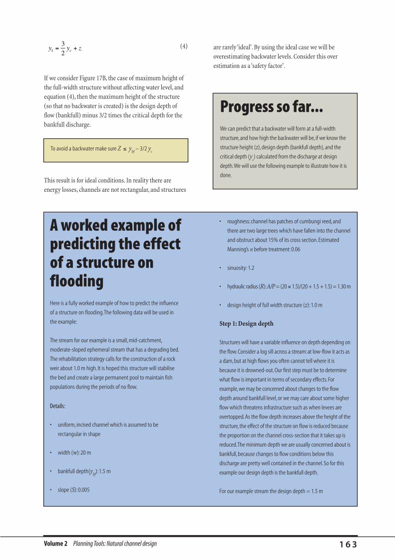
Volume 2 Planning Tools: Natural channel design 1 6 3
(4)
If we consider Figure 17B, the case of maximum height of
the full-width structure without affecting water level, and
equation (4), then the maximum height of the structure
(so that no backwater is created) is the design depth of
flow (bankfull) minus 3/2 times the critical depth for the
bankfull discharge.
This result is for ideal conditions. In reality there are
energy losses, channels are not rectangular, and structures
y y zc1
3
2= +
To avoid a backwater make sure Z ² ybf
– 3/2 yc
Progress so far...We can predict that a backwater will form at a full-width
structure, and how high the backwater will be, if we know the
structure height (z), design depth (bankfull depth), and the
critical depth (yc) calculated from the discharge at design
depth.We will use the following example to illustrate how it is
done.
A worked example ofpredicting the effectof a structure onfloodingHere is a fully worked example of how to predict the influence
of a structure on flooding.The following data will be used in
the example:
The stream for our example is a small, mid-catchment,
moderate-sloped ephemeral stream that has a degrading bed.
The rehabilitation strategy calls for the construction of a rock
weir about 1.0 m high. It is hoped this structure will stabilise
the bed and create a large permanent pool to maintain fish
populations during the periods of no flow.
Details:
• uniform, incised channel which is assumed to be
rectangular in shape
• width (w): 20 m
• bankfull depth(ybf
): 1.5 m
• slope (S): 0.005
• roughness: channel has patches of cumbungi reed, and
there are two large trees which have fallen into the channel
and obstruct about 15% of its cross section. Estimated
Manning’s n before treatment: 0.06
• sinuosity: 1.2
• hydraulic radius (R):A/P = (20 ´ 1.5)/(20 + 1.5 + 1.5) = 1.30 m
• design height of full width structure (z): 1.0 m
Step 1: Design depth
Structures will have a variable influence on depth depending on
the flow.Consider a log sill across a stream: at low-flow it acts as
a dam, but at high flows you often cannot tell where it is
because it is drowned-out.Our first step must be to determine
what flow is important in terms of secondary effects.For
example, we may be concerned about changes to the flow
depth around bankfull level, or we may care about some higher
flow which threatens infrastructure such as when levees are
overtopped.As the flow depth increases above the height of the
structure, the effect of the structure on flow is reduced because
the proportion on the channel cross-section that it takes up is
reduced.The minimum depth we are usually concerned about is
bankfull, because changes to flow conditions below this
discharge are pretty well contained in the channel.So for this
example our design depth is the bankfull depth.
For our example stream the design depth = 1.5 m
are rarely ‘ideal’. By using the ideal case we will be
overestimating backwater levels. Consider this over
estimation as a ‘safety factor’.

Volume 2 Planning Tools: Natural channel design 1 6 4
Step 2: Is the flow supercritical?
You will recall that supercritical flow is low depth, high velocity
(remember supercritical flow is like superman—faster than a
speeding bullet). If the flow is supercritical at bankfull discharge
and the full-width structure is not higher than bankfull, then no
backwater will be created.
As supercritical flow passes over a structure, it will have a local
increase in water depth, but by definition of supercritical flow,
this disturbance will not propagate upstream (Figure 18). In this
case the full-width structure acts simply as a bed roughness
feature.
Only steep gradient, shallow streams are likely to have
supercritical flow during bankfull conditions. For most streams,
the flow will be subcritical (deeper then critical depth) during
bankfull conditions.
For our example stream:
Use Manning’s equation to calculate the bankfull velocity
so v = 1.4 m/s
Now
when y = our design depth or bankfull (ybf
) = 1.5 m
For our stream, Fr = 0.37 which is less than one. Our flow is
therefore subcritical and we need to proceed to the next step
Step 3: Will the water depth increase when the
structure is built?
The accurate prediction of flow depths requires detailed analysis
of the channel and the shape of the full-width structure. For a
quick estimation we assume the channel is rectangular, and the
full-width structure is horizontal, with a flat surface like a broad-
crested weir. Using different shapes of full-width structure will
have only a small effect on water levels.The small variation in
water level is within the error bounds of this process so it is not
worth investigating alternative weir structures. So long as the
weir is not steeply angled into the channel like a V-notch weir
the predictions here are appropriate.
For our example stream:
The bankfull velocity calculated in the previous step = 1.4 m/s,
area A = 30 m2
therefore bankfull discharge (Qbf) = 42 m3/s
The critical depth for this flow is;
remember that the discharge per unit width for a rectangular
channel q = Q/w, ie.
yq
gc =æ
èç
ö
ø÷
2 1 3/
yc =æ
èç
ö
ø÷ =
( / )
..
/42 20
9 80 76
2 1 3
m
vR S
n
v
=
=
( / ) ( / )
( / ) ( / ). .
.
2 3 1 2
2 3 1 21 3 0 005
0 06
Frv
gy=
Fr =´
1 4
9 8 1 5
.
. .
Recall from earlier (equation 4) that if the structure influences
the upstream water depth, then flow over it will be at critical
depth (Figure 18) and the upstream water level will be 3/2
times the critical depth plus the structure height (Chadwick
and Morfett, 1993).
yc
Critical depth
Water level
Figure 18. Structures lower than critical depth will not form a backwater for supercritical flow.
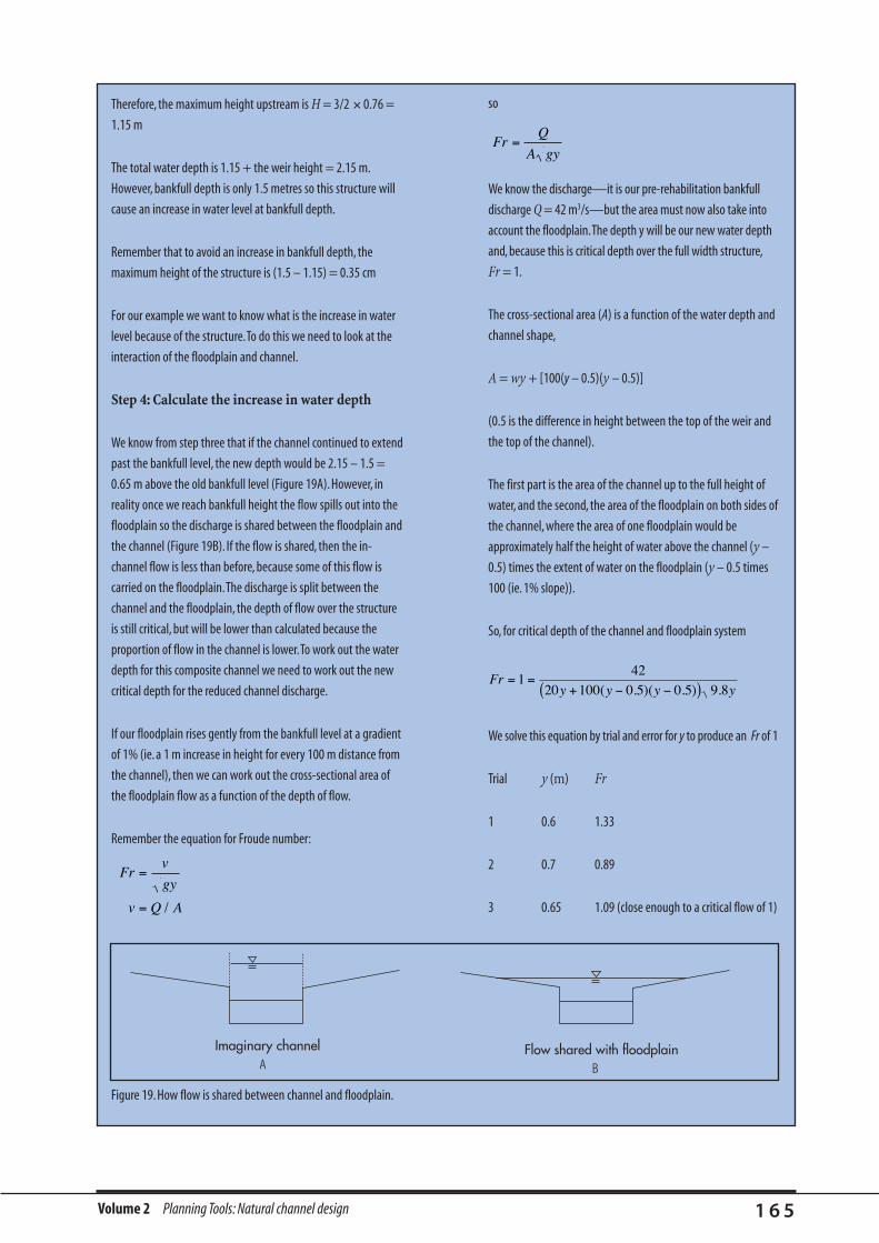
Volume 2 Planning Tools: Natural channel design 1 6 5
Therefore, the maximum height upstream is H = 3/2 ´ 0.76 =
1.15 m
The total water depth is 1.15 + the weir height = 2.15 m.
However, bankfull depth is only 1.5 metres so this structure will
cause an increase in water level at bankfull depth.
Remember that to avoid an increase in bankfull depth, the
maximum height of the structure is (1.5 – 1.15) = 0.35 cm
For our example we want to know what is the increase in water
level because of the structure.To do this we need to look at the
interaction of the floodplain and channel.
Step 4: Calculate the increase in water depth
We know from step three that if the channel continued to extend
past the bankfull level, the new depth would be 2.15 – 1.5 =
0.65 m above the old bankfull level (Figure 19A). However, in
reality once we reach bankfull height the flow spills out into the
floodplain so the discharge is shared between the floodplain and
the channel (Figure 19B). If the flow is shared, then the in-
channel flow is less than before, because some of this flow is
carried on the floodplain.The discharge is split between the
channel and the floodplain, the depth of flow over the structure
is still critical, but will be lower than calculated because the
proportion of flow in the channel is lower.To work out the water
depth for this composite channel we need to work out the new
critical depth for the reduced channel discharge.
If our floodplain rises gently from the bankfull level at a gradient
of 1% (ie. a 1 m increase in height for every 100 m distance from
the channel), then we can work out the cross-sectional area of
the floodplain flow as a function of the depth of flow.
Remember the equation for Froude number:
so
We know the discharge—it is our pre-rehabilitation bankfull
discharge Q = 42 m3/s—but the area must now also take into
account the floodplain.The depth y will be our new water depth
and, because this is critical depth over the full width structure,
Fr = 1.
The cross-sectional area (A) is a function of the water depth and
channel shape,
A = wy + [100(y – 0.5)(y – 0.5)]
(0.5 is the difference in height between the top of the weir and
the top of the channel).
The first part is the area of the channel up to the full height of
water, and the second, the area of the floodplain on both sides of
the channel, where the area of one floodplain would be
approximately half the height of water above the channel (y –
0.5) times the extent of water on the floodplain (y – 0.5 times
100 (ie. 1% slope)).
So, for critical depth of the channel and floodplain system
We solve this equation by trial and error for y to produce an Fr of 1
Trial y (m) Fr
1 0.6 1.33
2 0.7 0.89
3 0.65 1.09 (close enough to a critical flow of 1)
Frv
gy
v Q A
=
= /
FrQ
A gy=
Fry y y y
= =+ - -( )
142
20 100 0 5 0 5 9 8( . )( . ) .
Imaginary channel Flow shared with floodplain
Figure 19. How flow is shared between channel and floodplain.
A B

Volume 2 Planning Tools: Natural channel design 1 6 6
So the critical depth over the full-width structure is 65 cm:
therefore, the depth in the channel just upstream is 3/2 x 0.65 =
0.98 m: ie. the increased water level from the full-width
structures is about (0.98 – 0.5) 0.5 m when the floodplain flow is
also taken into account.
Step 5: Is this increased depth important?
If your full-width structure is likely to increase local water
depths, you need to consider the implications of the increase in
water depth and at what point it becomes a significant concern.
For this example we will say that the increase in depth is
acceptable, but we are concerned about how far upstream the
influence will extend.
Step 6: What is the extent of the backwater?
Estimate the backwater extent by assuming a horizontal line
from the water level just upstream of the weir until it reaches
design flow depth (ie. bankfull).
For our example,
The design flow depth is ybf
(y = 1.5 m)
the backwater is (1.98 – 1.5) ~ 0.5 m
the channel slope is 0.005 (assume the water surface without
the structure would have the same slope as the bed)
so the upstream extent of the backwater = 0.5/0.005 m
upstream extent is 100 m, but remember that the real extent will
be further upstream than this quick approximation.
Step 7: How much sooner will it now flood?
We have shown how to roughly estimate the increase in water
level for a given discharge when we place a full-width structure
in the channel, but an equally valuable question is how much
more frequently will out-of-bank flow (ie. flooding) occur
because of the structure? To answer this question we need a
time-series of stream flow so we can compare the frequency of
the current bankfull condition with the new bankfull condition.
In reality, such data are rarely available, but it is still valuable to
compare pre-rehabilitation and post-rehabilitation bankfull
discharges.
For our example stream,
the pre-rehabilitation discharge is 42 m3/s
from steps 3 and 4 above.The maximum post-rehabilitation in-
channel (ie. bankfull) discharge will occur when the water level is
at bankfull level and we have critical flow over the full-width
structure.Therefore, the depth of flow just upstream of the full-
width structure is 3/2 times the critical depth, or yc
= 2/3
(bankfull depth – structure height)
The only unknown is discharge, so we can solve the following by
trial and error to give the new bankfull discharge for a critical
depth of 0.33
We solve this equation by trial and error for Q
Trial Q (m3/s) yc
1 30 0.61
2 10 0.29
3 12 0.33 (this is the discharge
for critical depth)
Therefore, by placing a structure 1 m high in a 1.5 m deep
channel, the channel will now flow bankfull at just 12 m3/s
upstream of the structure, whereas before the treatment the
discharge was 42 m3/s before bankfull conditions were achieved.
In summary, we can estimate whether or not a full-width structure will have an influence on water depth by comparing the structure height plus
3/2 times the critical depth with the design height (bankfull). If we see that out-of-bank flow will occur we can predict the new depth of water for
simple cross-sections (including floodplain), based on critical depth over the full-width structure.
yq
gy zc bf=
æ
èç
ö
ø÷ = -
2 1 32
3
/
( )
yQ
c =æ
èç
ö
ø÷ = - =
( / )
.( . ) .
/20
9 8
2
31 5 1 0 333
2 1 3
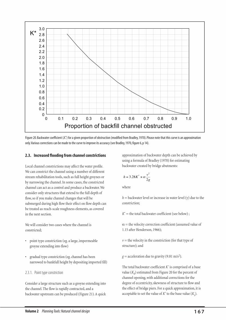
Volume 2 Planning Tools: Natural channel design 1 6 7
2.3. Increased flooding from channel constrictions
Local channel constrictions may affect the water profile.
We can constrict the channel using a number of different
stream rehabilitation tools, such as full height groynes or
by narrowing the channel. In some cases, the constricted
channel can act as a control and produce a backwater. We
consider only structures that extend to the full depth of
flow, so if you make channel changes that will be
submerged during high flow their effect on flow depth can
be treated as reach-scale roughness elements, as covered
in the next section.
We will consider two cases where the channel is
constricted;
• point type constriction (eg. a large, impermeable
groyne extending into flow)
• gradual type constriction (eg. channel has been
narrowed to bankfull height by depositing imported fill)
2.3.1. Point type constriction
Consider a large structure such as a groyne extending into
the channel. The flow is rapidly contracted, and a
backwater upstream can be produced (Figure 21). A quick
approximation of backwater depth can be achieved by
using a formula of Bradley (1970) for estimating
backwater created by bridge abutments:
where
h = backwater level or increase in water level (y) due to the
constriction;
K* = the total backwater coefficient (see below) ;
a = the velocity correction coefficient (assumed value of
1.15 after Henderson, 1966);
v = the velocity in the constriction (for that type of
structure); and
g = acceleration due to gravity (9.81 m/s2).
The total backwater coefficient K* is comprised of a base
value (Kb) estimated from Figure 20 for the percent of
channel opening, with additional corrections for the
degree of eccentricity, skewness of structure to flow and
the effect of bridge piers. For a quick approximation, it is
acceptable to set the value of K* to the base value (Kb).
h Kv
g= ´3 28
2
2
. * a
Figure 20. Backwater coefficient (K*) for a given proportion of obstruction (modified from Bradley, 1970). Please note that this curve is an approximation
only.Various corrections can be made to the curve to improve its accuracy (see Bradley, 1970, figure 6, p 14).

For points (1) and (2) in Figure 22, a backwater will be
formed when point (2) is narrow enough to create critical
flow depth.
Assuming no energy loss, the energy equation relating
point (1) and (2) is:
From the full-width structures section above this can be
rewritten as:
An example of the method is shown in the next box.
Volume 2 Planning Tools: Natural channel design 1 6 8
Figure 21.The dimensions of the groyne and channel under consideration.
Figure 22. Channel constriction can create a backwater.
y yc1
3
2=
A worked exampleof how to calculatethe backwatercreated by a groyneUsing the same stream as for the example in the previous
section, we will replace the full-width structure with a groyne
that extends 4 m into the channel.This gives a channel opening
of 80% or 0.8 (ie.16/20) of the full width.From Figure 20 this
gives a Kb value of 0.55, which we will adopt for the K* value.
a = 1.15
Calculate v as the average velocity through the opening using
Manning’s equation assuming the flow depth to be bankfull at
the obstruction.
The hydraulic radius is now (16 ´ 1.5/(16 + 1.5 + 1.5)) = 1.26
so v = 1.4 m/s
Now calculate the backwater
h = 0.207 m, or a backwater of 21 cm (that is, the water
surface elevation upstream of the groyne increases by 21 cm).
vR S
n=
( / ) ( / )2 3 1 2
v =1 326 0 005
0 06
2 3 1 2. .
.
( / ) ( . )
20m16m
Groyne
Plan
16m20m
1.5m
Groyne
Flow
Cross-section
2.3.2. Gradual channel constriction
The smooth transition from a wider to narrower cross-
section can result in critical flow depth at the new cross-
section if the channel has been sufficiently constricted.
(Figure 22). The production of a backwater in this case is
the same mechanism as for a full-width structure. In both
cases the structure reduces the channel cross-sectional
area, critical flow depth occurs in the constriction, and a
backwater is formed upstream of the constriction.
h kv
g
h
= ´
= ´ ´´
3 282
3 28 0 55 1 151 4
2 9 8
2
2
.
. . ..
.
* a
Critical depth at constriction
Channel constricted
Old wide channel
yc
Elevation
Plan
Depth
Flow
yv
gy
v
gcc
112 2
2 2+ = +
1 2
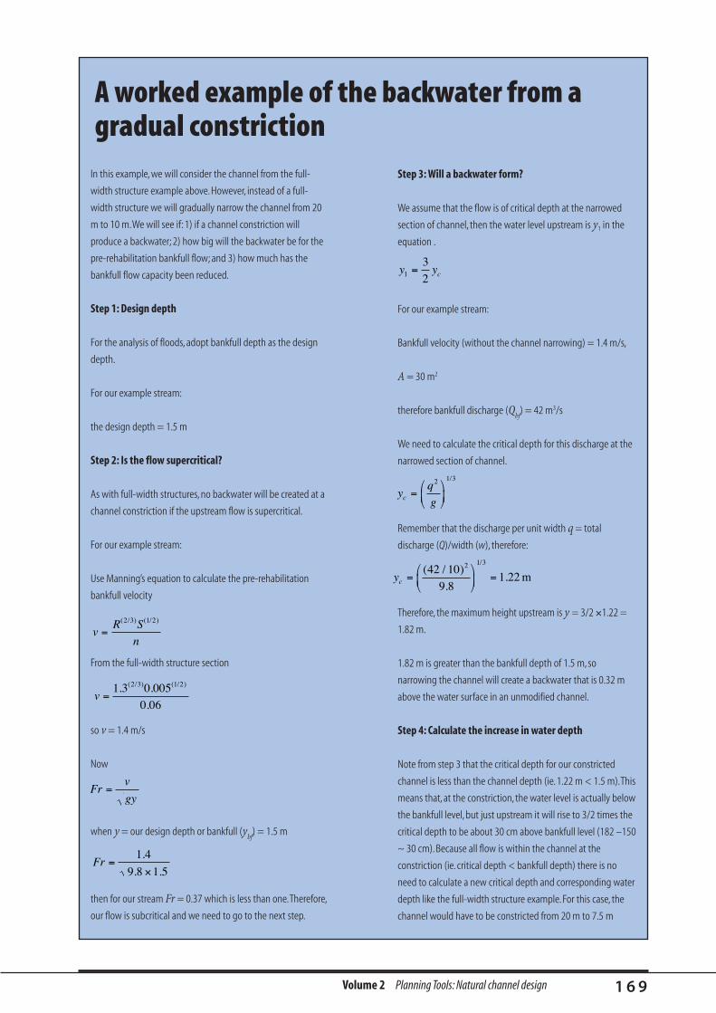
Volume 2 Planning Tools: Natural channel design 1 6 9
In this example, we will consider the channel from the full-
width structure example above. However, instead of a full-
width structure we will gradually narrow the channel from 20
m to 10 m.We will see if: 1) if a channel constriction will
produce a backwater; 2) how big will the backwater be for the
pre-rehabilitation bankfull flow; and 3) how much has the
bankfull flow capacity been reduced.
Step 1: Design depth
For the analysis of floods, adopt bankfull depth as the design
depth.
For our example stream:
the design depth = 1.5 m
Step 2: Is the flow supercritical?
As with full-width structures, no backwater will be created at a
channel constriction if the upstream flow is supercritical.
For our example stream:
Use Manning’s equation to calculate the pre-rehabilitation
bankfull velocity
From the full-width structure section
so v = 1.4 m/s
Now
when y = our design depth or bankfull (ybf
) = 1.5 m
then for our stream Fr = 0.37 which is less than one.Therefore,
our flow is subcritical and we need to go to the next step.
Step 3: Will a backwater form?
We assume that the flow is of critical depth at the narrowed
section of channel, then the water level upstream is y1 in the
equation .
For our example stream:
Bankfull velocity (without the channel narrowing) = 1.4 m/s,
A = 30 m2
therefore bankfull discharge (Qbf
) = 42 m3/s
We need to calculate the critical depth for this discharge at the
narrowed section of channel.
Remember that the discharge per unit width q = total
discharge (Q)/width (w), therefore:
Therefore, the maximum height upstream is y = 3/2 ´1.22 =
1.82 m.
1.82 m is greater than the bankfull depth of 1.5 m, so
narrowing the channel will create a backwater that is 0.32 m
above the water surface in an unmodified channel.
Step 4: Calculate the increase in water depth
Note from step 3 that the critical depth for our constricted
channel is less than the channel depth (ie. 1.22 m < 1.5 m).This
means that, at the constriction, the water level is actually below
the bankfull level, but just upstream it will rise to 3/2 times the
critical depth to be about 30 cm above bankfull level (182 –150
~ 30 cm). Because all flow is within the channel at the
constriction (ie. critical depth < bankfull depth) there is no
need to calculate a new critical depth and corresponding water
depth like the full-width structure example. For this case, the
channel would have to be constricted from 20 m to 7.5 m
vR S
n=
( / ) ( / )2 3 1 2
v =1 3 0 005
0 06
2 3 1 2. .
.
( / ) ( / )
Frv
gy=
Fr =´
1 4
9 8 1 5
.
. .
y yc1
3
2=
yq
gc =æ
èç
ö
ø÷
2 1 3/
yc =æ
èç
ö
ø÷ =
( / )
..
/42 10
9 81 22
2 1 3
m
A worked example of the backwater from agradual constriction

Volume 2 Planning Tools: Natural channel design 1 7 0
before the critical depth exceeds the bankfull depth and we
need to calculate a new critical depth including floodplain flow,
like we did for the full-width structure example.
Step 5: Is this increased depth important?
Consider the influence of the effect of an increase in the local
water level, and what it may affect. For the sake of our example
we will say that 30 cm is of concern, so we will consider the
upstream extent.
Step 6: What is the extent of the backwater?
Estimate the backwater extent by assuming a horizontal line
from the water level just upstream of the constriction until it
reaches bankfull flow depth.
For our example:
The design flow depth is bankfull (y = 1.5 m)
the backwater is 0.32 m
the channel slope is 0.005 (assume the water surface has the
same slope)
so the upstream extent of the backwater = 0.32/0.005
upstream extent is 64 m
remember that this is the absolute minimum extent of
backwater
Step 7: How much sooner will it now flood?
We have shown how to roughly estimate the increase in water
level for a given discharge when we constrict the channel but
an equally valuable question is how much have we reduced the
channel capacity by constricting it? The answer is the same as
for step 7 in the example of calculating the backwater for a full
width structure.
For our example stream:
the pre-rehabilitation discharge is 42 m3/s.
From steps 3 and 4 above, the maximum post-rehabilitation in-
channel (ie. bankfull) discharge will occur when the water level
is at bankfull level and we have critical flow through the
constriction.Therefore, the depth of flow just upstream of the
full-width structure is 3/2 times the critical depth, or yc
= 2/3
(bankfull depth)
the unknown is discharge, so we can solve the following by trial
and error to give the new bankfull discharge
We solve this equation by trial and error for Q
trial Q (m3/s) yc
1 40 1.17
2 25 0.86
3 30 0.97 (close enough)
Therefore, by constricting the channel width from 20 m to 10
m, the channel will now flow bankfull at 30 m3/s whereas
before the treatment the bankfull discharge was 42 m3/s.
yq
gyc bf=
æ
èç
ö
ø÷ =
2 1 32
3
/
yQ
c =æ
èç
ö
ø÷ = ´ =
( / )
.. .
/10
9 8
2
31 5 1 0
2 1 3
2.4. Flooding from increased channel roughness
In the case of reduced channel capacity from increased
roughness, individual roughness elements (eg. individual
snags) do not produce a noticeable backwater, but the
cumulative effect of the elements reduces the capacity of
the channel, and water depth is subsequently increased for
a given discharge. If we think about stream energy being
either kinetic energy (related to flow velocity) or potential
energy (related to flow depth), channel roughness causes
kinetic energy loss through turbulent flow around the
roughness elements. Hence, a greater energy in the form of
flow depth is required for the same discharge to
compensate for the lost kinetic energy.
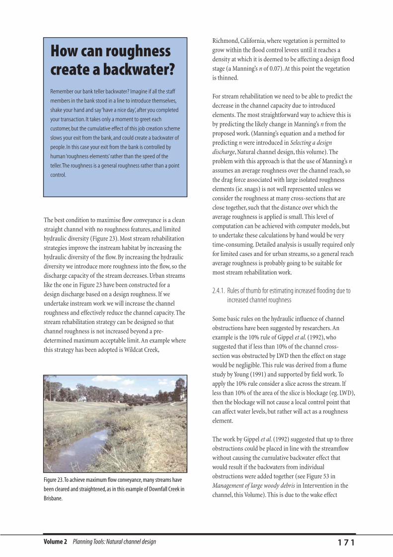
Volume 2 Planning Tools: Natural channel design 1 7 1
The best condition to maximise flow conveyance is a clean
straight channel with no roughness features, and limited
hydraulic diversity (Figure 23). Most stream rehabilitation
strategies improve the instream habitat by increasing the
hydraulic diversity of the flow. By increasing the hydraulic
diversity we introduce more roughness into the flow, so the
discharge capacity of the stream decreases. Urban streams
like the one in Figure 23 have been constructed for a
design discharge based on a design roughness. If we
undertake instream work we will increase the channel
roughness and effectively reduce the channel capacity. The
stream rehabilitation strategy can be designed so that
channel roughness is not increased beyond a pre-
determined maximum acceptable limit. An example where
this strategy has been adopted is Wildcat Creek,
Richmond, California, where vegetation is permitted to
grow within the flood control levees until it reaches a
density at which it is deemed to be affecting a design flood
stage (a Manning’s n of 0.07). At this point the vegetation
is thinned.
For stream rehabilitation we need to be able to predict the
decrease in the channel capacity due to introduced
elements. The most straightforward way to achieve this is
by predicting the likely change in Manning’s n from the
proposed work. (Manning’s equation and a method for
predicting n were introduced in Selecting a design
discharge, Natural channel design, this volume). The
problem with this approach is that the use of Manning’s n
assumes an average roughness over the channel reach, so
the drag force associated with large isolated roughness
elements (ie. snags) is not well represented unless we
consider the roughness at many cross-sections that are
close together, such that the distance over which the
average roughness is applied is small. This level of
computation can be achieved with computer models, but
to undertake these calculations by hand would be very
time-consuming. Detailed analysis is usually required only
for limited cases and for urban streams, so a general reach
average roughness is probably going to be suitable for
most stream rehabilitation work.
2.4.1. Rules of thumb for estimating increased flooding due toincreased channel roughness
Some basic rules on the hydraulic influence of channel
obstructions have been suggested by researchers. An
example is the 10% rule of Gippel et al. (1992), who
suggested that if less than 10% of the channel cross-
section was obstructed by LWD then the effect on stage
would be negligible. This rule was derived from a flume
study by Young (1991) and supported by field work. To
apply the 10% rule consider a slice across the stream. If
less than 10% of the area of the slice is blockage (eg. LWD),
then the blockage will not cause a local control point that
can affect water levels, but rather will act as a roughness
element.
The work by Gippel et al. (1992) suggested that up to three
obstructions could be placed in line with the streamflow
without causing the cumulative backwater effect that
would result if the backwaters from individual
obstructions were added together (see Figure 53 in
Management of large woody debris in Intervention in the
channel, this Volume). This is due to the wake effect
Figure 23.To achieve maximum flow conveyance, many streams have
been cleared and straightened, as in this example of Downfall Creek in
Brisbane.
How can roughnesscreate a backwater?Remember our bank teller backwater? Imagine if all the staff
members in the bank stood in a line to introduce themselves,
shake your hand and say ‘have a nice day’, after you completed
your transaction. It takes only a moment to greet each
customer, but the cumulative effect of this job creation scheme
slows your exit from the bank, and could create a backwater of
people. In this case your exit from the bank is controlled by
human ‘roughness elements’ rather than the speed of the
teller.The roughness is a general roughness rather than a point
control.

Volume 2 Planning Tools: Natural channel design 1 7 2
behind an in-channel object, which shields a downstream
obstruction from the direct force of the flow. The same
could be said for a groyne or retard field where the first
structure has a pronounced effect on flow hydraulics but
subsequent structures simply maintain rather than add to
the altered flow conditions. Gippel’s 10% rule is applied for
isolated obstructions. However, if stream rehabilitation
occurs on a reach scale it is convenient to consider reduced
channel capacity in terms of an increase in the average
reach roughness. The following examples illustrate how to
do this using Manning’s equation. Shields and Gippel
(1995) provide a more accurate approach for assessing the
hydraulic effect of LWD.
2.4.2. Examples of increased roughness
Let us consider three examples of stream rehabilitation
works in which general roughness will increase:
• bendway weirs are added to an upper catchment stream
• an artificial bench is formed to move the point of attack
away from an eroding bend (this differs from the
constriction example because the bench does not
extend the full height of the channel)
• revegetation of the banks of the channel in Figure 23.
Calculating the effectof increasedroughness caused bybendway weirs onchannel flow capacityThis is a real example, from a rehabilitation site on Pappinbarra
Creek, a tributary of the Nambucca River on then north coast of
New South Wales.
The stream has the following characteristics:
width = 25 m
depth = 0.8 m
bed slope = 0.01
sinuosity Å1.2 at the point of works
bed material = gravel and cobble D50
Å 20 mm
bendway weirs = logs ~ 0.3 m diameter, that extend about 8
m into the channel
Step 1: What is the design depth?
As previous for examples, we will adopt the bankfull height as
the design depth; ie.y = 0.8 m.
Step 2: What is the pre-rehabilitation Manning’s n?
To select a pre-rehabilitation Manning’s n we will compare n
values from Chow’s table, and from Cowan’s method (see
Selecting a design discharge in Natural channel design, this volume
for a discussion of Manning’s n and the relevant tables).
From Chow’s table: we have a ‘natural stream: clean, winding,
some pools and shoals, some weeds and stones’, normal n
value = 0.045
According to Cowan’s method, we can estimate components of
Manning’s n for bankfull flow.
Material n0
0.028 (coarse gravel)
Irregularity n1
0.005 (minor irregularity)
Cross-section n2
0.000 (gradual cross section
variations)
Obstructions n3
0.000 (no obstructions)
Vegetation n4
0.010 (low vegetation)
Meandering m 1 (low sinuosity)
Manning’s n = (n0 + n
1+ n
2+n
3+ n
4)m
Therefore, for this channel during bankfull conditions
Manning’s n from Cowan’s method is 0.043
The Chow and Cowan Manning’s ns compare well: n is set at 0.045
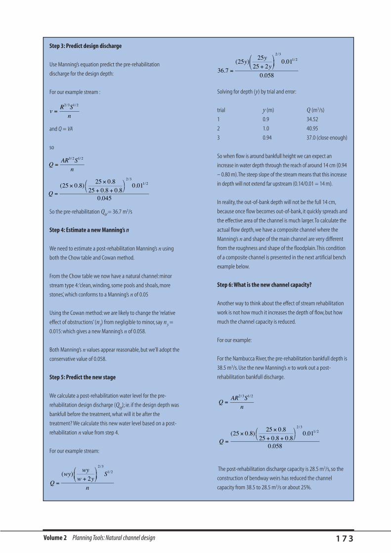
Volume 2 Planning Tools: Natural channel design 1 7 3
Step 3: Predict design discharge
Use Manning’s equation predict the pre-rehabilitation
discharge for the design depth:
For our example stream :
and Q = VA
so
So the pre-rehabilitation Qbf
= 36.7 m3/s
Step 4: Estimate a new Manning’s n
We need to estimate a post-rehabilitation Manning’s n using
both the Chow table and Cowan method.
From the Chow table we now have a natural channel: minor
stream type 4:‘clean, winding, some pools and shoals, more
stones’, which conforms to a Manning’s n of 0.05
Using the Cowan method: we are likely to change the ‘relative
effect of obstructions’ (n3) from negligible to minor, say n
3=
0.015: which gives a new Manning’s n of 0.058.
Both Manning’s n values appear reasonable, but we’ll adopt the
conservative value of 0.058.
Step 5: Predict the new stage
We calculate a post-rehabilitation water level for the pre-
rehabilitation design discharge (Qbf
); ie. if the design depth was
bankfull before the treatment, what will it be after the
treatment? We calculate this new water level based on a post-
rehabilitation n value from step 4.
For our example stream:
Solving for depth (y) by trial and error:
trial y (m) Q (m3/s)
1 0.9 34.52
2 1.0 40.95
3 0.94 37.0 (close enough)
So when flow is around bankfull height we can expect an
increase in water depth through the reach of around 14 cm (0.94
– 0.80 m).The steep slope of the stream means that this increase
in depth will not extend far upstream (0.14/0.01 = 14 m).
In reality, the out-of-bank depth will not be the full 14 cm,
because once flow becomes out-of-bank, it quickly spreads and
the effective area of the channel is much larger.To calculate the
actual flow depth, we have a composite channel where the
Manning’s n and shape of the main channel are very different
from the roughness and shape of the floodplain.This condition
of a composite channel is presented in the next artificial bench
example below.
Step 6: What is the new channel capacity?
Another way to think about the effect of stream rehabilitation
work is not how much it increases the depth of flow, but how
much the channel capacity is reduced.
For our example:
For the Nambucca River, the pre-rehabilitation bankfull depth is
38.5 m3/s. Use the new Manning’s n to work out a post-
rehabilitation bankfull discharge.
The post-rehabilitation discharge capacity is 28.5 m3/s, so the
construction of bendway weirs has reduced the channel
capacity from 38.5 to 28.5 m3/s or about 25%.
vR S
n=
2 3 1 2/ /
QAR S
n=
3 2 1 2/ /
Q =´
´+ +
æè
öø
( . ).
. ..
.
//25 0 8
25 0 825 0 8 0 8
0 01
0 045
2 31 2
Q
wywy
w yS
n=
+
æ
èç
ö
ø÷( )
/
/
2
2 3
1 2
36 7
2525
25 20 01
0 058
2 3
1 2
.
( ) .
.
/
/
=+
æ
èç
ö
ø÷y
y
y
Q =´
´+ +
æè
öø
( . ).
. ..
.
//25 0 8
25 0 825 0 8 0 8
0 01
0 058
2 31 2
QAR S
n=
2 3 1 2/ /
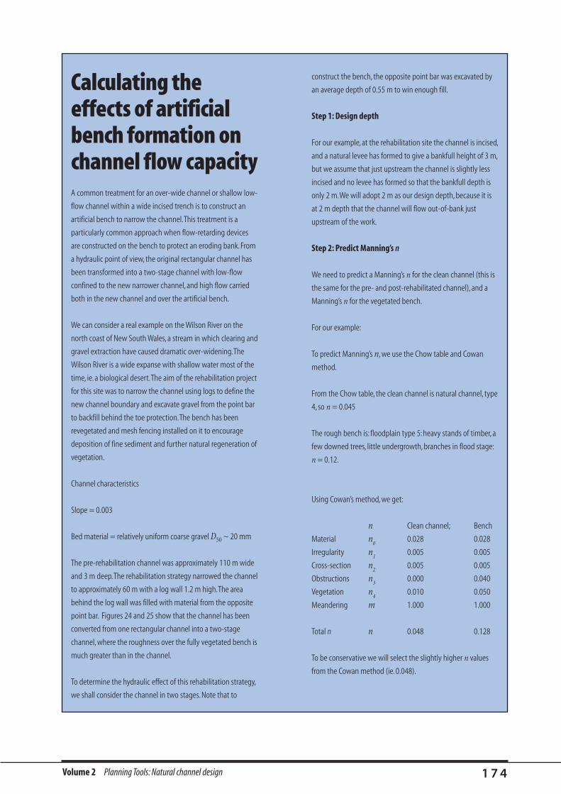
Volume 2 Planning Tools: Natural channel design 1 7 4
Calculating theeffects of artificialbench formation onchannel flow capacityA common treatment for an over-wide channel or shallow low-
flow channel within a wide incised trench is to construct an
artificial bench to narrow the channel.This treatment is a
particularly common approach when flow-retarding devices
are constructed on the bench to protect an eroding bank. From
a hydraulic point of view, the original rectangular channel has
been transformed into a two-stage channel with low-flow
confined to the new narrower channel, and high flow carried
both in the new channel and over the artificial bench.
We can consider a real example on the Wilson River on the
north coast of New South Wales, a stream in which clearing and
gravel extraction have caused dramatic over-widening.The
Wilson River is a wide expanse with shallow water most of the
time, ie. a biological desert.The aim of the rehabilitation project
for this site was to narrow the channel using logs to define the
new channel boundary and excavate gravel from the point bar
to backfill behind the toe protection.The bench has been
revegetated and mesh fencing installed on it to encourage
deposition of fine sediment and further natural regeneration of
vegetation.
Channel characteristics
Slope = 0.003
Bed material = relatively uniform coarse gravel D50 ~ 20 mm
The pre-rehabilitation channel was approximately 110 m wide
and 3 m deep.The rehabilitation strategy narrowed the channel
to approximately 60 m with a log wall 1.2 m high.The area
behind the log wall was filled with material from the opposite
point bar. Figures 24 and 25 show that the channel has been
converted from one rectangular channel into a two-stage
channel, where the roughness over the fully vegetated bench is
much greater than in the channel.
To determine the hydraulic effect of this rehabilitation strategy,
we shall consider the channel in two stages. Note that to
construct the bench, the opposite point bar was excavated by
an average depth of 0.55 m to win enough fill.
Step 1: Design depth
For our example, at the rehabilitation site the channel is incised,
and a natural levee has formed to give a bankfull height of 3 m,
but we assume that just upstream the channel is slightly less
incised and no levee has formed so that the bankfull depth is
only 2 m.We will adopt 2 m as our design depth, because it is
at 2 m depth that the channel will flow out-of-bank just
upstream of the work.
Step 2: Predict Manning’s n
We need to predict a Manning’s n for the clean channel (this is
the same for the pre- and post-rehabilitated channel), and a
Manning’s n for the vegetated bench.
For our example:
To predict Manning’s n, we use the Chow table and Cowan
method.
From the Chow table, the clean channel is natural channel, type
4, so n = 0.045
The rough bench is: floodplain type 5: heavy stands of timber, a
few downed trees, little undergrowth, branches in flood stage:
n = 0.12.
Using Cowan’s method, we get:
n Clean channel; Bench
Material n0
0.028 0.028
Irregularity n1
0.005 0.005
Cross-section n2
0.005 0.005
Obstructions n3
0.000 0.040
Vegetation n4
0.010 0.050
Meandering m 1.000 1.000
Total n n 0.048 0.128
To be conservative we will select the slightly higher n values
from the Cowan method (ie. 0.048).

Volume 2 Planning Tools: Natural channel design 1 7 5
Figure 24.The creation of an artificial bench on the Wilson River.
Figure 25. A schematic diagram of the sediment moved to form the Wilson River bench.
110m
50m 60m
1.2m
3m
1.8m
Pre-rehabilitation channel
Post-rehabilitation channel
50m 60m
1.2mnb
Fill2.35m 3.55m
Old channel
110m
3mCut
na
Assume constant n for full width Assume different Manning's n values for themain channel and the revegetated bench
Pre–rehabilitation Post–rehabilitation
Step 3: Pre-rehabilitation discharge
Use Manning’s equation to work out the pre-rehabilitation
bankfull discharge;
For our example:
and Q = VA
so
Therefore, for our design depth, Q = 390 m3/s
Step 4: What is the depth of the design flow in the
rehabilitated channel?
To predict the depth of the design flow in the post-
rehabilitation channel we simply combine the two sections of
the channel and solve for the depth by trial and error.
For our example:
If the depth of water in the main channel is y, then the depth
over the bench is y –1.2 m.
Note that the wetted perimeter for the sections is only that
depth that is in contact with bank or bed material (ie. not the
water interface between the two sections).
Q =´
´+ +
æè
öø
110 2110 2
110 2 20 003
0 048
2 31 2
//.
.
vR S
n=
2 3 1 2/ /
QAR S
n=
2 3 1 2/ /
Q SA R
n
A R
n= +
æ
èç
ö
ø÷
1 2 1 12 3
1
2 22 3
2
/( / ) ( / )
390 0 003
50 1 250 1 250 1 2
0 128
6060
60 1 2
0 0481 2
2 3 2 3
=
-( ) -+ -
æ
èç
ö
ø÷
++ +
æ
èç
ö
ø÷
æ
è
çççç
ö
ø
÷÷÷÷
.
( . )( . )
.
.
( ).
./
/ /
yy
yy
y
y
Bench section Clean channel section
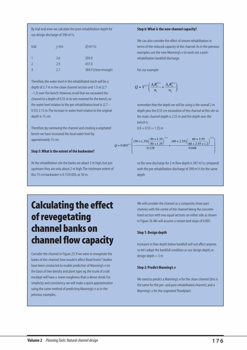
Volume 2 Planning Tools: Natural channel design 1 7 6
By trial and error we calculate the post-rehabilitation depth for
our design discharge of 390 m3/s.
trial y (m) Q (m3/s)
1 2.6 359.9
2 2.9 437.0
3 2.7 384.9 (close enough)
Therefore, the water level in the rehabilitated reach will be a
depth of 2.7 m in the clean channel section and 1.5 m (2.7
–1.2) over the bench. However, recall that we excavated the
channel to a depth of 0.55 m to win material for the bench, so
the water level relative to the pre-rehabilitation level is (2.7 –
0.55) 2.15 m.The increase in water level relative to the original
depth is 15 cm.
Therefore, by narrowing the channel and creating a vegetated
bench we have increased the local water level by
approximately 15 cm.
Step 5: What is the extent of the backwater?
At the rehabilitation site the banks are about 3 m high, but just
upstream they are only about 2 m high.The minimum extent of
this 15 cm backwater is 0.15/0.003, or 50 m.
Step 6: What is the new channel capacity?
We can also consider the effect of stream rehabilitation in
terms of the reduced capacity of the channel. As in the previous
examples, use the new Manning’s n to work out a post-
rehabilitation bankfull discharge.
For our example:
remember that the depth we will be using is the overall 2 m
depth plus the 0.55 cm excavation of the channel at this site so
the main channel depth is 2.55 m and the depth over the
bench is
0.8 + 0.55 = 1.35 m
so the new discharge for 2 m flow depth is 347 m3/s, compared
with the pre-rehabilitation discharge of 390 m3/s for the same
depth
Q SA R
n
A R
n= +
æ
èç
ö
ø÷
1 2 1 12 3
1
2 22 3
2
// /
Q =´
´+
æè
öø
+´
´+ +
æè
öø
æ
è
ççç
ö
ø
÷÷÷
0 00350 1 35
50 1 3550 1 35
0 128
60 2 5560 2 55
60 2 55 1 20 048
1 2
2 3 2 3
.( . )
.
..
( . ).
. ..
/
/ /
Calculating the effectof revegetatingchannel banks onchannel flow capacityConsider the channel in Figure 23. If we were to revegetate the
banks of this channel, how would it affect flood levels? Studies
have been conducted to enable prediction of Manning’s n on
the basis of tree density and plant type; eg. the trunk of a tall
eucalypt will have a lower roughness than a dense shrub. For
simplicity and consistency we will make a quick approximation
using the same method of predicting Manning’s n as in the
previous examples.
We will consider the channel as a composite, three-part
channel, with the centre of the channel being the concrete-
lined section with two equal sections on either side as shown
in Figure 26.We will assume a stream bed slope of 0.005.
Step 1: Design depth
Increases in flow depth below bankfull will not affect anyone,
so let’s adopt the bankfull condition as our design depth, ie.
design depth = 3 m
Step 2: Predict Manning’s n
We need to predict a Manning’s n for the clean channel (this is
the same for the pre- and post-rehabilitated channel), and a
Manning’s n for the vegetated ‘floodplain’.
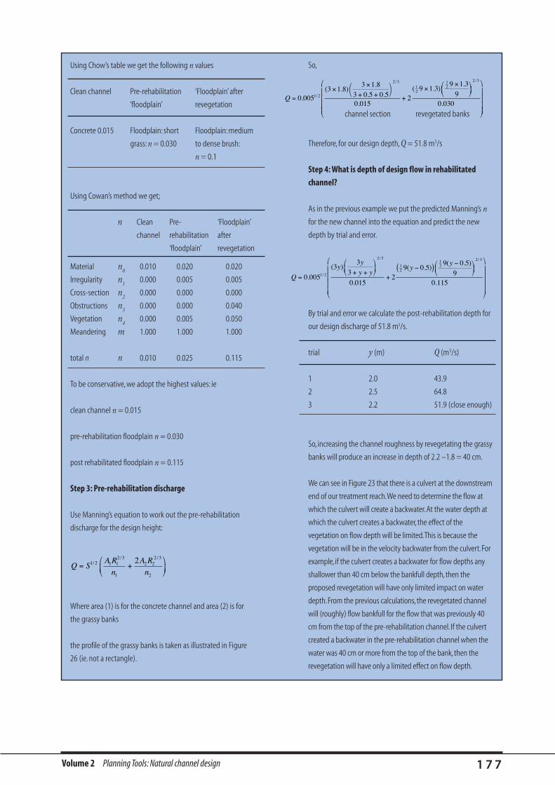
Volume 2 Planning Tools: Natural channel design 1 7 7
Using Chow’s table we get the following n values
Clean channel Pre-rehabilitation ‘Floodplain’ after
‘floodplain’ revegetation
Concrete 0.015 Floodplain: short Floodplain: medium
grass: n = 0.030 to dense brush:
n = 0.1
Using Cowan’s method we get;
n Clean Pre- ‘Floodplain’
channel rehabilitation after
‘floodplain’ revegetation
Material n0
0.010 0.020 0.020
Irregularity n1
0.000 0.005 0.005
Cross-section n2
0.000 0.000 0.000
Obstructions n3
0.000 0.000 0.040
Vegetation n4
0.000 0.005 0.050
Meandering m 1.000 1.000 1.000
total n n 0.010 0.025 0.115
To be conservative, we adopt the highest values: ie
clean channel n = 0.015
pre-rehabilitation floodplain n = 0.030
post rehabilitated floodplain n = 0.115
Step 3: Pre-rehabilitation discharge
Use Manning’s equation to work out the pre-rehabilitation
discharge for the design height:
Where area (1) is for the concrete channel and area (2) is for
the grassy banks
the profile of the grassy banks is taken as illustrated in Figure
26 (ie. not a rectangle).
So,
Therefore, for our design depth, Q = 51.8 m3/s
Step 4: What is depth of design flow in rehabilitated
channel?
As in the previous example we put the predicted Manning’s n
for the new channel into the equation and predict the new
depth by trial and error.
By trial and error we calculate the post-rehabilitation depth for
our design discharge of 51.8 m3/s.
trial y (m) Q (m3/s)
1 2.0 43.9
2 2.5 64.8
3 2.2 51.9 (close enough)
So, increasing the channel roughness by revegetating the grassy
banks will produce an increase in depth of 2.2 –1.8 = 40 cm.
We can see in Figure 23 that there is a culvert at the downstream
end of our treatment reach.We need to determine the flow at
which the culvert will create a backwater.At the water depth at
which the culvert creates a backwater, the effect of the
vegetation on flow depth will be limited.This is because the
vegetation will be in the velocity backwater from the culvert.For
example, if the culvert creates a backwater for flow depths any
shallower than 40 cm below the bankfull depth,then the
proposed revegetation will have only limited impact on water
depth.From the previous calculations, the revegetated channel
will (roughly) flow bankfull for the flow that was previously 40
cm from the top of the pre-rehabilitation channel. If the culvert
created a backwater in the pre-rehabilitation channel when the
water was 40 cm or more from the top of the bank, then the
revegetation will have only a limited effect on flow depth.
Q SA R
n
A R
n= +
æ
èç
ö
ø÷
1 2 1 12 3
1
2 22 3
2
2// /
Q
yy
y yy
y
=+ +
æ
èç
ö
ø÷
+-( ) -æ
èç
öø÷
æ
è
çççç
ö
ø
÷÷÷÷
0 005
33
3
0 0152
9 0 59 0 5
90 115
1 2
2 3
12
12
2 3
.
( )
.
( . )( . )
./
/ /
Q =´
´+ +
æè
öø
+´
´æèç
öø÷
æ
è
çççç
ö
ø
÷÷÷÷
0 0053 1 8
3 1 83 0 5 0 50 015
29 1 3
9 1 39
0 0301 2
2 312
12
2 3
.( . )
.. .
.
( . ).
./
/ /
channel section revegetated banks

Volume 2 Planning Tools: Natural channel design 1 7 8
3m 9m9m
0.5m
Pre-rehabilitation channel Post-rehabilitation channel: same dimensions butdifferent roughness in-channel and on ‘floodplain’
1.8m
Figure 26. A schematic of the pre- and post-rehabilitation channel for Downfall Creek.

EVALUATION TOOLS
• Evaluation
Volume 2 Planning Tools: Evaluation tools 1 8 0
Evaluation is an extremely important step in the
rehabilitation procedure. With no formal check on the
success of a project, it is difficult to improve the techniques
we use, because we don’t even know if they need
improving. Through evaluation we can also learn more
about little-known aspects of stream systems, such as the
habitat preferences of fish. The regular monitoring
involved in evaluation also means that damage, or flaws in
the project, can often be detected and fixed, where
otherwise they may have gone unnoticed.
Although there is no doubt that evaluation is extremely
useful, it is extremely rare. This is largely because no one
likes to find out that their hard work resulted in failure,
especially not to admit it in public. Even if you do decide to
bite the bullet and evaluate your work, thorough evaluation
can be time-consuming, expensive, and difficult.
There are ways of getting around these dismal-looking
problems. Realistically, a stream rehabilitation project
should be seen as an experiment (Kondolf and Micheli,
1995). Then there is no shame in admitting that one or all
goals were not met. There is a lot to be learnt from failures.
Also, not all evaluations need be difficult and expensive
(although this tends to be the case for the more
informative designs). By limiting your ambitions, it is
possible to do a quick and easy evaluation.
This chapter is an extension of Step 10: How will you
evaluate your project? in the Stream rehabilitation planning
procedure in Volume 1. The chapter consists of three
sections. Fundamentals of evaluation design will give you a
basic understanding of why people are fussy about the
design of evaluations. Planning the evaluation of a
rehabilitation project presents 11 tasks that help you
develop your evaluation plan. This section also provides
information for Step 7 of the Rehabilitation procedure in
Volume 1: Setting objectives. Finally, Evaluation case studies
presents several real examples of evaluation.
EVALUATION
Even if you do decide to opt for a simple type of
evaluation, it is good to understand and appreciate the
reasons why a thorough evaluation can be tricky and time-
consuming. This basic knowledge will also help you
understand the limits of any evaluation.
The two basic questions we ask in every evaluation are: 1)
"has something really changed"; and 2) "is the change that
we are seeing really caused by our actions, or is it caused
by something else?" Natural systems are always
undergoing change, because they are constantly
responding to changes in numerous environmental
influences (eg. temperature or rainfall).Any impact of our
actions is superimposed onto this constant background of
change. Designing an experiment to identify what changes
are related to our intervention is a specialised and
laborious task that entertains the days of scientists. For a
more detailed discussion of experimental design see
Gordon et al. (1992), or Underwood (1996). The main
purpose of this section is to introduce you to some
principles of experimental design that will help you to
appreciate why scientists are so careful about it. It also aims
to encourage you to think very hard about experimental
design before being tempted to measure things.
1. Fundamentals of evaluation design
Is there a difference between monitoring andevaluation?Yes. Monitoring is the collection of information about the effectiveness of a treatment. Evaluation is the assessment of that monitoring—that is,
deciding what the results of your monitoring tell you about the success or failure of the project.Thus, many projects are monitored but never
evaluated, because nobody does anything with the monitoring information.
Volume 2 Planning Tools: Evaluation tools 1 8 1
1.1. Natural variation
Natural systems are always in a state of change. There are
regular fluctuations such as daily and seasonal change,
and more random variation in response to chance
occurrences, such as a flood, or a particularly warm winter.
Variation also occurs spatially. For example, plant species
found in the upper catchment are usually different from
those in the lower reaches. Some species of
macroinvertebrate live on large, clean rocks while others in
the same stream will live in the finer sediment between
rocks. It is the temporal and spatial variation intrinsic to
natural systems that makes experimental design critical to
successful evaluation of your project. If your experimental
design is the skeleton of the evaluation plan, then your
sampling methodology is the meat on the bones.
1.1.1.Spatial variation
Ideally, if you wanted to know what macroinvertebrates
were present in a stream, or the particle size distribution
on a gravel bar, you would count every individual animal
or stone. That way, you could be sure the result of your
survey accurately represented what was really present in
the stream. Obviously, this will almost never be possible.
Instead, you must take samples—a net-full of
invertebrates, or a shovel-full of sediment.You then count
the animals or stones in that sample, and assume that the
sample is representative of the entire population of
invertebrates, or all the sediment in the gravel bar. This is
all very well, so long as the macroinvertebrates are
distributed evenly through the stream, and the size of the
gravel does not vary across the bar. Here you are out of
luck. Macroinvertebrates are not distributed evenly—
different species will live in different habitats, and even
within the same habitat some areas may be more densely
populated than others. Gravel is not distributed evenly
across a bar—the upstream end tends to be coarser
sediment, and there is also the possibility of armouring.
The solution to this problem is to take several sub-samples
from different parts of the stream at that site. From these,
you can calculate an average, which we assume to be
First some definitions:
Evaluation plan The detailed plan of how you do your experiment—what you measure, when, how often, etc.
Treatment or This is the thing that you do to the stream (in this case, some stream rehabilitation activity).
intervention
Control This is a sampling site or reach which as similar as possible to the rehabilitation site in every way, except that
it is not rehabilitated. The control site is compared with the rehabilitation site as a way of checking that any
changes are a result of the rehabilitation, rather than some other unconnected event affecting the whole
stream.
Uncontrolled Does not refer to a lack of discipline, rather it refers to a project that has no control site or reach.
experiment
Replication This is repeat sampling to identify the inherent variability in the system.You can have replicates on many
scales—replicate rivers to see if the results can be applied to different streams; replicate study sites within a
river to see of all reaches react in the same way; replicate samples over time, to measure the temporal
variability, and replicate sub-samples within a sample, to measure spatial variability. Thus, when you sample,
you might take 10 samples from the reach instead of one, or 10 samples from 10 streams at the same time.
Sample A measurement of some sort. It could be anything from the average depth of erosion at a site, as measured by
erosion pins, to a measure of water quality, or a survey of the invertebrate population at a site.
Sub-sampling Sometimes, a sample is made up of many sub-samples. For example, if you wanted to know the rate of
erosion at one site, you might use several erosion pins. The sub-samples would be the individual pins, and
the sample would be the average rate of erosion around all the pins at the site. This means you can estimate
how much variation there is at any one site.
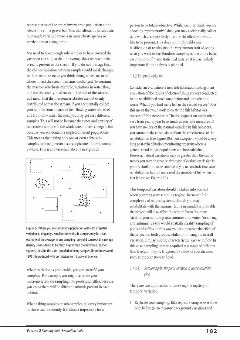
representative of the entire invertebrate population at the
site, or the entire gravel bar. This also allows us to calculate
how much variation there is in invertebrate species or
particle size at a single site.
You need to take enough sub-samples to have covered the
variation at a site, so that the average does represent what
is really present in the stream. If you do not manage this,
the chance variation between samples could mask changes
in the stream, or make you think changes have occurred
where in fact the stream remains unchanged. To continue
the macroinvertebrate example, variations in water flow,
and the size and type of rocks on the bed of the stream,
will mean that the macroinvertebrates are not evenly
distributed across the stream. If you accidentally collect
your sample from an area of fast-flowing water one week,
and from slow water the next, you may get very different
samples. This will not be because the types and density of
macroinvertebrates in the whole stream have changed, but
because you accidentally sampled different populations.
This means that taking only one or even a few sub-
samples may not give an accurate picture of the stream as
a whole. This is shown schematically in Figure 27.
Volume 2 Planning Tools: Evaluation tools 1 8 2
Figure 27.Where you are sampling a population with a lot of spatial
variation, taking only a small number of sub-samples may be a bad
estimate of the average.In one sampling run (solid squares), the average
density is considered to be much higher than the next time (dashed
squares), despite the same population being sampled (from Underwood,
1996).Reproduced with permission from Blackwell Science.
Where variation is predictable, you can ‘stratify’ your
sampling. For example, you might separate your
macroinvertebrate sampling into pools and riffles, because
you know there will be different animals present in each
habitat.
When taking samples or sub-samples, it is very important
to chose each randomly. It is almost impossible for a
person to be totally objective. While you may think you are
choosing ‘representative’ sites, you may accidentally collect
data which are more likely to show the effect you would
like to be present. This does not imply deliberate
falsification of results, just the very human trait of seeing
what you want to see. Random sampling is one of the basic
assumptions of many statistical tests, so it is particularly
important if any analysis is planned.
1.1.2.Temporal variation
Consider an evaluation of new fish habitat, consisting of an
evaluation of the results of electro-fishing surveys conducted
in the rehabilitated reach once before and once after the
works.What if you find more fish in the second survey? Does
this mean that your work to create the fish habitat was
successful? Not necessarily. The fish population might often
vary from year to year by as much as you have measured. If
you have no idea of the natural variation in fish numbers,
you cannot make conclusions about the effectiveness of the
rehabilitation (see Figure 28A).An exception would be a very
long post-rehabilitation monitoring program where a
general trend in fish populations can be established.
However, natural variations may be greater than the subtle
trends you may observe, so this type of evaluation design is
poor.A similar mistake could lead you to conclude that your
rehabilitation has not increased the number of fish when in
fact it has (see Figure 28B).
This temporal variation should be taken into account
when planning your sampling regime. Because of the
complexity of natural systems, though you may
rehabilitate with the summer fauna in mind, it is probable
the project will also affect the winter fauna.You may
‘stratify’ your sampling into summer and winter (or spring
and autumn), as you would spatially stratify sampling of
pools and riffles. In this way you can measure the effect of
the project on both groups, while minimising the overall
variation. Similarly, some characteristics vary with flow. In
this case, sampling may be required at a range of different
flow levels, or may be triggered by a flow of specific size,
such as the 5 or 10-year flood.
1.1.2.A. Accounting for temporal variation in your evaluation plan
There are two approaches to removing the mystery of
temporal variation:
1. Replicate your sampling. Take replicate samples over time
both before (ie. to measure background variation) and
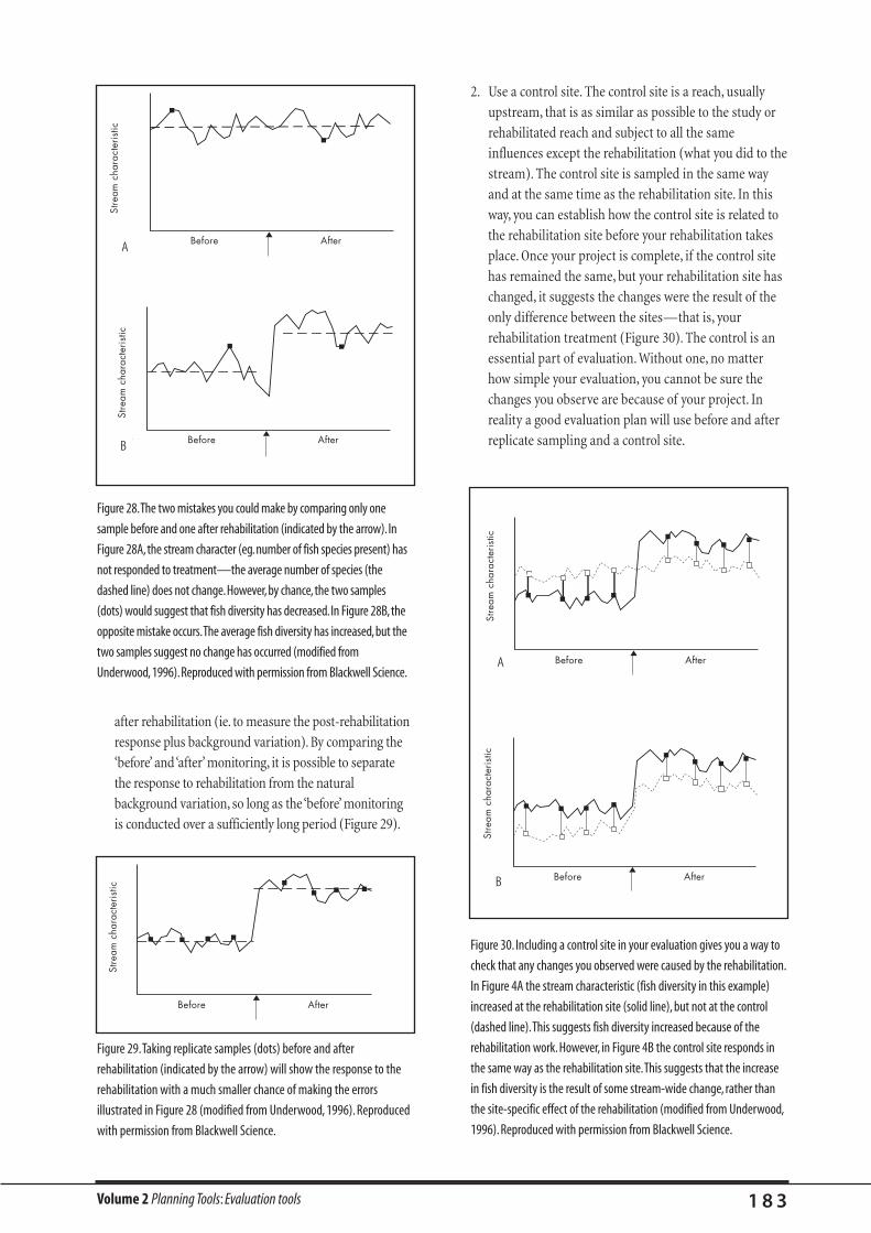
Volume 2 Planning Tools: Evaluation tools 1 8 3
2. Use a control site. The control site is a reach, usually
upstream, that is as similar as possible to the study or
rehabilitated reach and subject to all the same
influences except the rehabilitation (what you did to the
stream). The control site is sampled in the same way
and at the same time as the rehabilitation site. In this
way, you can establish how the control site is related to
the rehabilitation site before your rehabilitation takes
place. Once your project is complete, if the control site
has remained the same, but your rehabilitation site has
changed, it suggests the changes were the result of the
only difference between the sites—that is, your
rehabilitation treatment (Figure 30). The control is an
essential part of evaluation. Without one, no matter
how simple your evaluation, you cannot be sure the
changes you observe are because of your project. In
reality a good evaluation plan will use before and after
replicate sampling and a control site.
Figure 29.Taking replicate samples (dots) before and after
rehabilitation (indicated by the arrow) will show the response to the
rehabilitation with a much smaller chance of making the errors
illustrated in Figure 28 (modified from Underwood, 1996). Reproduced
with permission from Blackwell Science.
Before After
Stre
am c
hara
cter
istic
after rehabilitation (ie. to measure the post-rehabilitation
response plus background variation). By comparing the
‘before’ and ‘after’ monitoring, it is possible to separate
the response to rehabilitation from the natural
background variation, so long as the ‘before’ monitoring
is conducted over a sufficiently long period (Figure 29).
Figure 28.The two mistakes you could make by comparing only one
sample before and one after rehabilitation (indicated by the arrow).In
Figure 28A,the stream character (eg.number of fish species present) has
not responded to treatment—the average number of species (the
dashed line) does not change.However,by chance,the two samples
(dots) would suggest that fish diversity has decreased.In Figure 28B,the
opposite mistake occurs.The average fish diversity has increased,but the
two samples suggest no change has occurred (modified from
Underwood,1996).Reproduced with permission from Blackwell Science.
Before After
Stre
am c
hara
cter
istic
(a)
Before After
Stre
am c
hara
cter
istic
(b)
A
B
Before After
Stre
am c
hara
cter
istic
Before After
Stre
am c
hara
cter
istic
Figure 30. Including a control site in your evaluation gives you a way to
check that any changes you observed were caused by the rehabilitation.
In Figure 4A the stream characteristic (fish diversity in this example)
increased at the rehabilitation site (solid line), but not at the control
(dashed line).This suggests fish diversity increased because of the
rehabilitation work.However, in Figure 4B the control site responds in
the same way as the rehabilitation site.This suggests that the increase
in fish diversity is the result of some stream-wide change, rather than
the site-specific effect of the rehabilitation (modified from Underwood,
1996). Reproduced with permission from Blackwell Science.
B
A

Volume 2 Planning Tools: Evaluation tools 1 8 4
1.2. Choosing the best sample size (power analysis,or how small a change do I want to detect?)
When deciding how many samples to take, time and money
constraints suggest less is better. However, there is a
problem with this. The fewer samples you take, the less
chance you have of detecting any change your
rehabilitation makes, particularly if there is a lot of
variation between samples. Look again at Figures 28 and
29.When comparing only two samples, the differences in
the true average were hidden, but the average of four
samples was more representative of the real situation, and
the differences were apparent. So, the power of your
evaluation (chance of detecting a given change) depends
upon how many samples you take, and how much variation
exists between them. It is possible to calculate how much
power you have (see Coehn, 1988). This can be very useful.
You may find that in a very variable stream system, such as
urban streams, for example, an evaluation including only a
few samples would have the power to detect only huge
changes to the stream that would be easily visible without a
full scientific study. In this case, you may decide to find
more money and increase the number of samples, or not to
bother with this style of evaluation.
1.3. What makes a robust evaluation?
The need for a practical evaluation approach that will deal
with natural and spatial variability has led to the
development of BACI (Before–After/Control–Impact). This
is an evaluation program with two sites (rehabilitation and
control), with replicate samples taken through time, and
replicate sub-samples taken each time you sample. This
replicated BACI design is a quite robust evaluation
technique. However, there is still the possibility that the
difference between the control and rehabilitation sites was
due to a chance event not connected to the experiment,
and the conclusion that the rehabilitation project had
made a difference would be wrong. In fact it is the rule,
rather than the exception, that some extraneous
circumstance will arise during the evaluation period (eg. a
landholder downstream of the control site constructs a
ford across the stream and blocks fish passage, or a gravel
extraction plant starts up in the control site and raises the
turbidity levels, or cattle are allowed to graze the control
site because of a severe drought). The solution to this
problem is to go ‘beyond BACI’, and have several control
reaches (controls on your control). If possible, it is also
advantageous to rehabilitate more than one reach. This
results in the most robust design for your evaluation, as
there is very little chance that the results could be caused
by an unfortunate chance occurrence. It also provides
baseline data for future projects which deal with the same
sorts of problems.
1.4. What can evaluation tell you?
The most basic purpose of evaluation is to tell you if your
rehabilitation project has succeeded or failed, according to
your objectives. However, a well-designed evaluation will
also give you something just as important —that is, the
reasons for those results. This is the most informative part
of evaluation, where you examine what aspects of the
rehabilitation projects worked (fish did utilise the LWD
habitat), and what aspects caused failure (the target species
of fish were still rare in the reach, because they were out-
competed by carp). It is this information that will help you
improve and refine your rehabilitation techniques.
Bear in mind that distributing credit for success, or
blame for failure, is much harder when the rehabilitation
project consists of many different changes, all with their
own effects. Unfortunately, most rehabilitation projects
fall into this category. For example, consider a project
that involved adding woody debris to the stream,
constructing an artificial riffle to increase
macroinvertebrate density (the favoured food of the
target fish), removing the fish barrier downstream and
an electro-fishing program to selectively remove carp
Some rules ofevaluationRule 1: Always have a control to check for natural fluctuations.
Rule 2:To account for spatial variation:
• stratify (take separate samples from different seasons or
areas); and
• take sub-samples.
Rule 3:To account for temporal variation:
• replicate (take samples at more than one time); and
• include a control.
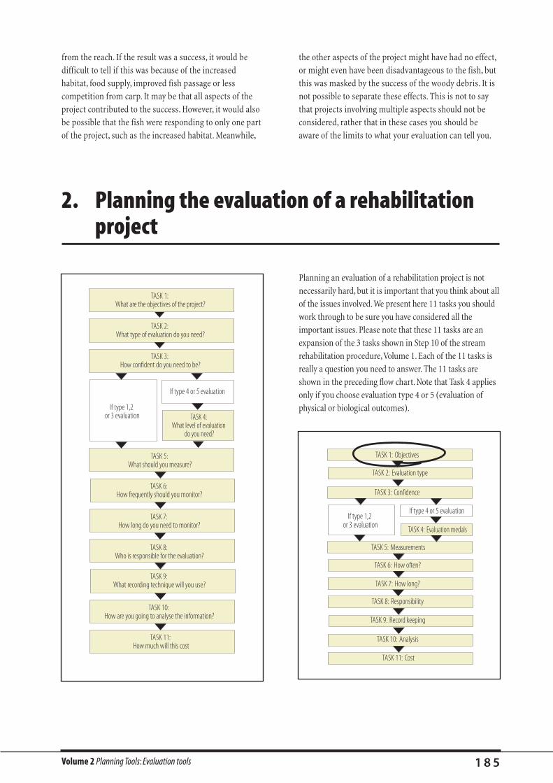
Volume 2 Planning Tools: Evaluation tools 1 8 5
from the reach. If the result was a success, it would be
difficult to tell if this was because of the increased
habitat, food supply, improved fish passage or less
competition from carp. It may be that all aspects of the
project contributed to the success. However, it would also
be possible that the fish were responding to only one part
of the project, such as the increased habitat. Meanwhile,
the other aspects of the project might have had no effect,
or might even have been disadvantageous to the fish, but
this was masked by the success of the woody debris. It is
not possible to separate these effects. This is not to say
that projects involving multiple aspects should not be
considered, rather that in these cases you should be
aware of the limits to what your evaluation can tell you.
Planning an evaluation of a rehabilitation project is not
necessarily hard, but it is important that you think about all
of the issues involved.We present here 11 tasks you should
work through to be sure you have considered all the
important issues. Please note that these 11 tasks are an
expansion of the 3 tasks shown in Step 10 of the stream
rehabilitation procedure,Volume 1. Each of the 11 tasks is
really a question you need to answer. The 11 tasks are
shown in the preceding flow chart. Note that Task 4 applies
only if you choose evaluation type 4 or 5 (evaluation of
physical or biological outcomes).
2. Planning the evaluation of a rehabilitation project
TASK 1: What are the objectives of the project?
TASK 2: What type of evaluation do you need?
TASK 3: How confident do you need to be?
TASK 5: What should you measure?
TASK 6: How frequently should you monitor?
TASK 7: How long do you need to monitor?
TASK 8: Who is responsible for the evaluation?
TASK 9: What recording technique will you use?
TASK 10: How are you going to analyse the information?
TASK 11: How much will this cost
TASK 4: What level of evaluation
do you need?
If type 4 or 5 evaluation
If type 1,2 or 3 evaluation
TASK 1: Objectives
TASK 2: Evaluation type
TASK 3: Confidence
TASK 11: Cost
TASK 5: Measurements
TASK 6: How often?
TASK 7: How long?
TASK 8: Responsibility
TASK 9: Record keeping
TASK 10: Analysis
TASK 4: Evaluation medals
If type 4 or 5 evaluationIf type 1,2
or 3 evaluation
Volume 2 Planning Tools: Evaluation tools 1 8 6
Table 25.Types of objectives for stream rehabilitation.
Output/ Type of objective Example of objectives
outcomes
Output Execution of the project. • Fence 7–10 km of stream, and provide two off-stream watering points by next summer.
Output Survival of the project. • Flood gates in the fence survived a 5-year flood.
• A core of people still attend Rivercare meetings after 3 years.
Outcome Aesthetics of the stream. • Revegetation inside the fence makes the stream look much more attractive after 5 years.
Outcome Changes in the physical • After five years, the pools would be between 20 and 50% deeper.
or chemical condition of the • The riparian vegetation will provide between 1 and 10 fragments of woody debris per kilometre
stream (may relate to the of stream per year, after 20 years.
riparian zone, the physical
form, the hydrology or the
water quality).
Outcome Improvement or • The range of species present (diversity) in the riparian zone will be between 50 and 100% of
maintenance of stream that found in the template reach after 5 years.
ecology. • The numbers of a particular organism (eg. platypus, fish, macroinvertebrates, redgum) will
increase to between 20 and 60% of populations found in the template reach after 4 years.
2.1. Task 1: What are the objectives of the project?
The first rule of evaluation is that you be very clear what it
is that you are evaluating. In Step 7: What are you specific
rehabilitation objectives? of the Stream rehabilitation
planning procedure,Volume 1, you should have developed
clear objectives for your rehabilitation project. The success
of the rehabilitation project is therefore measured by how
closely the conditions of the rehabilitated stream meet
those specified in the objectives.
Consider a project to increase fish populations by
replacing LWD in a reach devoid of habitat. The objective
should be as specific as possible. Rather than stating the
objective as merely to increase fish numbers, you should
consider if you are interested in all fish, or just certain
species, perhaps popular angling fish, or maybe not just
fish but macroinvertebrates as well.You should also
consider by how much you wish to increase the
population. Would you consider the project a success if
there were only three more fish in the reach? The
objectives you end up with may be something like "to
increase the trout cod population in this reach by 50% in 5
years". Objectives must often be couched in terms of
events of given probability. For example, this structure
should survive a flood of 10-year average recurrence
interval. If you expect a change in response to a particular
flow regime, it is only reasonable to wait for that flow to
occur before you can declare the project a success or
failure (we will consider the importance of flow variability
in Tasks 6 and 7: How frequently and How long should you
monitor?).
Briefly, objectives should specify the following.
• How much change you want to see as a result of the
rehabilitation.
• What length of stream you want to improve.
• How long you will wait before concluding the evaluation.
You should also have considered whether your objectives
relate to outputs (tasks to be completed), or outcomes (the
effect on the stream of those tasks), and what type of
objective you have (Table 25). Table 26 provides some
examples of how to turn general objectives into
measurable objectives.
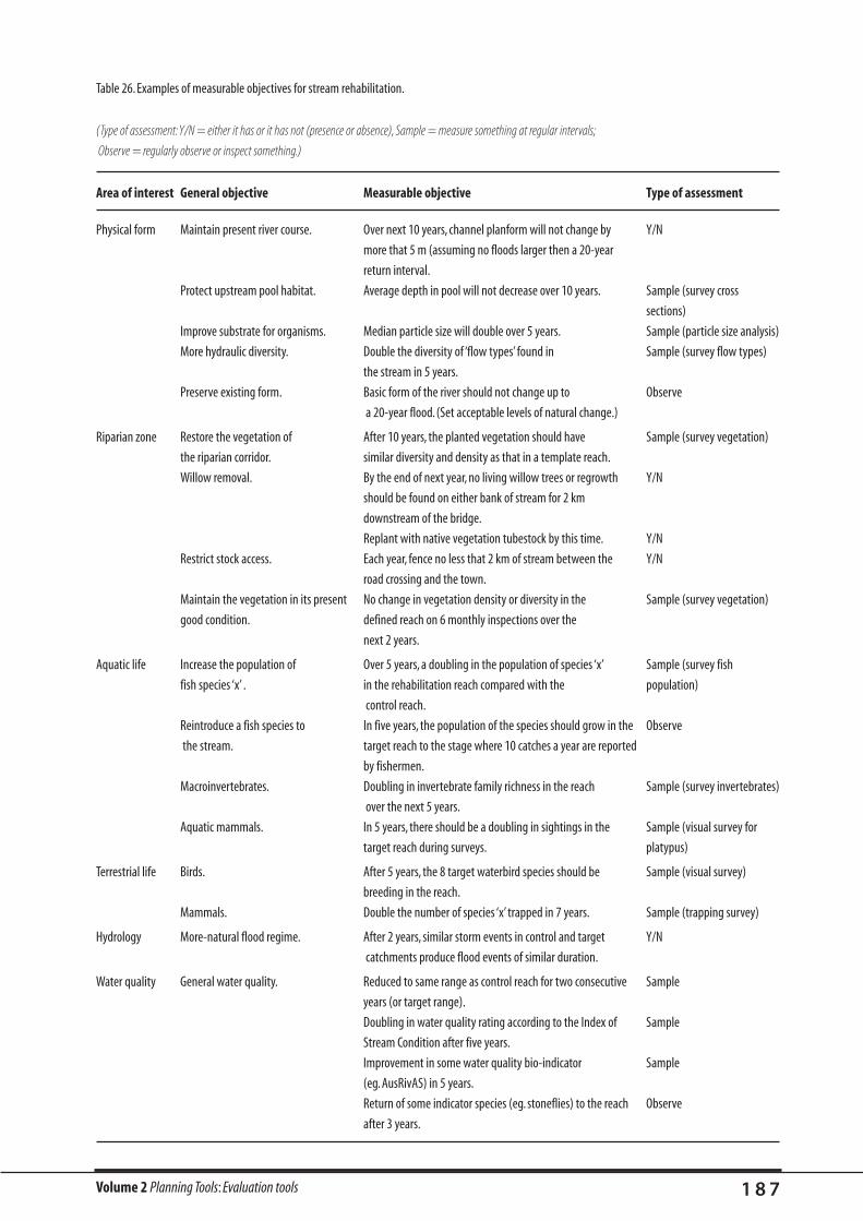
Volume 2 Planning Tools: Evaluation tools 1 8 7
Table 26. Examples of measurable objectives for stream rehabilitation.
(Type of assessment:Y/N = either it has or it has not (presence or absence), Sample = measure something at regular intervals;
Observe = regularly observe or inspect something.)
Area of interest General objective Measurable objective Type of assessment
Physical form Maintain present river course. Over next 10 years, channel planform will not change by Y/N
more that 5 m (assuming no floods larger then a 20-year
return interval.
Protect upstream pool habitat. Average depth in pool will not decrease over 10 years. Sample (survey cross
sections)
Improve substrate for organisms. Median particle size will double over 5 years. Sample (particle size analysis)
More hydraulic diversity. Double the diversity of ‘flow types’ found in Sample (survey flow types)
the stream in 5 years.
Preserve existing form. Basic form of the river should not change up to Observe
a 20-year flood. (Set acceptable levels of natural change.)
Riparian zone Restore the vegetation of After 10 years, the planted vegetation should have Sample (survey vegetation)
the riparian corridor. similar diversity and density as that in a template reach.
Willow removal. By the end of next year, no living willow trees or regrowth Y/N
should be found on either bank of stream for 2 km
downstream of the bridge.
Replant with native vegetation tubestock by this time. Y/N
Restrict stock access. Each year, fence no less that 2 km of stream between the Y/N
road crossing and the town.
Maintain the vegetation in its present No change in vegetation density or diversity in the Sample (survey vegetation)
good condition. defined reach on 6 monthly inspections over the
next 2 years.
Aquatic life Increase the population of Over 5 years, a doubling in the population of species ‘x’ Sample (survey fish
fish species ‘x’ . in the rehabilitation reach compared with the population)
control reach.
Reintroduce a fish species to In five years, the population of the species should grow in the Observe
the stream. target reach to the stage where 10 catches a year are reported
by fishermen.
Macroinvertebrates. Doubling in invertebrate family richness in the reach Sample (survey invertebrates)
over the next 5 years.
Aquatic mammals. In 5 years, there should be a doubling in sightings in the Sample (visual survey for
target reach during surveys. platypus)
Terrestrial life Birds. After 5 years, the 8 target waterbird species should be Sample (visual survey)
breeding in the reach.
Mammals. Double the number of species ‘x’ trapped in 7 years. Sample (trapping survey)
Hydrology More-natural flood regime. After 2 years, similar storm events in control and target Y/N
catchments produce flood events of similar duration.
Water quality General water quality. Reduced to same range as control reach for two consecutive Sample
years (or target range).
Doubling in water quality rating according to the Index of Sample
Stream Condition after five years.
Improvement in some water quality bio-indicator Sample
(eg. AusRivAS) in 5 years.
Return of some indicator species (eg. stoneflies) to the reach Observe
after 3 years.

Volume 2 Planning Tools: Evaluation tools 1 8 8
2.2. Task 2: What type of evaluation do you need? 2.2.1.Type 1:Execution outputs
Funding bodies often define evaluation as being evidence
that the works were executed according to plan. That is, the
money was spent on the things it was supposed to be spent
on. This is a simple accounting process, but should not be
confused with other levels of evaluation. Execution means
simply checking that the job was or was not done
according to design: "the fences were built, the drop
structure was put in on time, but we only put in six of the
eight retards…". This type of evaluation is useful as an
ongoing record of works, but is only the starting point for
other levels of evaluation. It assumes that if the structures
are there or the works are done then the project will be a
success.
2.2.2.Type 2:Survival outputs
Has your project survived? This is the most common form
of evaluation, and certainly the minimum that should be
expected. It is an extension of execution type evaluation in
that the existence of the structures implies your objectives
have been achieved. For example, after the 1993 floods in
north-eastern Victoria, the success of various structures
was measured by whether they were still there after the
flood. If they were, they were deemed to have succeeded
(AVRMA, 1994). But this does not prove that the structures
were successful; it can lead to no more than an assumption
that they were.
Survival-type evaluation requires repeat surveys to see how
the works are performing. It would usually start with a
detailed ‘execution’-type survey with follow-up reviews at
either preset intervals or on the basis of flood events. For
example, say we installed log sills to increase pool habitat.
The first phase of the evaluation (execution) is to verify
they have been installed as designed. This is then followed
by an event-based survival evaluation which records if the
sills have survived any flood greater than, for example, a 2-
year return interval. This type of evaluation is very
important for in-stream structures, as it helps us to identify
the structures that are suitable for different stream types.
Sometimes it is also possible to identify why the
rehabilitation has not succeeded (eg. "rabbits ate the
plants", "seepage destroyed the structure because no geo-
textile was used").
TASK 1: Objectives
TASK 2: Evaluation type
TASK 3: Confidence
TASK 11: Cost
TASK 5: Measurements
TASK 6: How often?
TASK 7: How long?
TASK 8: Responsibility
TASK 9: Record keeping
TASK 10: Analysis
TASK 4: Evaluation medals
If type 4 or 5 evaluationIf type 1,2
or 3 evaluation
You will develop your evaluation plan differently
depending on the type of objective that you have. There are
five types of evaluation that mirror the types of objective
described in Table 25. These are described below,
presented in order of complexity from the simplest type of
evaluation to the most complex. Select the evaluation type
that most suits the objectives for your project.
Note that the different types of evaluation are not mutually
exclusive. Most projects have a series of objectives (like
milestones), relating to different outputs and outcomes. In
fact, it can be quite useful to incorporate all types of
evaluation. This means you can keep track of the condition
of your rehabilitation structures (and be ready with
maintenance when required), as well as monitoring the
effect they have on the physical or biological nature of the
stream. Also, the different types of evaluation typically
occur over different time frames, as discussed in Task 7
(How long do you need to monitor?). For example,
evaluating execution can be done as soon as the works are
completed, but you might have to wait 10 years to complete
the evaluation of the biological outcomes of the work.
Because of this, including different types of evaluation will
mean regular reporting of progress, and help to keep the
community interested in the project.

Volume 2 Planning Tools: Evaluation tools 1 8 9
2.2.3.Type 3:Aesthetic outcomes
In many cases, the objectives of a stream rehabilitation
project relate most strongly to aesthetics—that the stream
should ‘look’ better or more natural. These objectives are
the easiest to evaluate. Obviously, aesthetics is in the eye of
the beholder, but it is pretty easy to come to a consensus.
The same is true for most rehabilitation that involves
replacing infestations of exotic vegetation with native
vegetation eg. clearing blackberries, water weeds, or
willows.
The key thing to remember about this type of evaluation
by ‘opinion’ is that people have short memories.You must
somehow record the original condition of the stream so
that you do not have to rely on memory.Video recorders
are good for this purpose, as are copious photographs.
Remember the cost of a film is small compared with the
cost of the project.
2.2.4.Type 4:Physical and chemical outcomes
Although the goal of rehabilitation is often to improve the
ecological condition of the stream, this is usually done by
improving the structural and chemical condition of the
stream (eg. hydraulic habitat, LWD density, scour holes,
substrate composition, water quality etc.). These physical
changes are cheaper and easier to measure than the
biological systems that they are meant to influence. As a
result, most evaluation is targeted at these changes, and it
is simply assumed that a biological response will follow.
The key problem with this type of evaluation is to ensure
that the change that you are measuring is related to your
rehabilitation, and not to some other change in the stream.
This problem is discussed below in Task 4: What level of
evaluation design do you need?
2.2.5.Type 5:Ecological outcomes
Ecological improvement is the vision driving almost all
stream rehabilitation projects. However, evaluating
ecological outcomes is not as common as you might think.
This is partly because we usually attempt to manipulate
stream ecology by changing the physical or chemical
nature of the stream, so evaluating success at that level
often seems sufficient. Also, monitoring ecological change
can be difficult, and take considerably longer than other
types of evaluation. Ecological evaluations most
commonly measure changes in the types, abundance and
diversity of the species present (eg. are there fish present,
how many fish are present, how many species of fish are
present, what are the fish species present?).
As with evaluations measuring physical changes, it is very
important to ensure that the change that you are
measuring is related to your rehabilitation efforts, and not
due to some unrelated change in the stream. This problem
is discussed below in Task 4: What level of evaluation
design do you need?
Evaluation ofsurvival: V-log sillsin northern NewSouth WalesFrom notes provided by David Outhet, John Bucinskas and Wal Hader (NSW,
DLWC)
The Nambucca River, in the mid-north coast of New South
Wales has suffered severe degradation since European
settlement in the area. In an attempt to stabilise the gravel bed
of the stream, 66 log sills were constructed. After some floods,
48 of the structures were inspected to assess if they had
survived. Most had been outflanked, scoured from below, or
covered in sediment.
These are some of the lessons learned from the structures that
survived.
• Locate the structure on a straight reach or inflection point
so that it does not get outflanked.
• V-logs should be used only on gravel-bed streams because
downstream scour will undermine the structure in sand-
bed streams.
• Straight log sills perform better than V-sills.

Volume 2 Planning Tools: Evaluation tools 1 9 0
An example of a Type 4 evaluationA rehabilitation project on Little Butte Creek, in south-western Oregon, USA, aimed to increase the number of trout present in the stream by
increasing the habitat available (Maiyo,1996) .Table 27 shows the physical effects of the project by comparing the original condition with the
post-project condition, as well as measuring some of the morphological changes produced by the project. As with execution and survival-type
evaluations, this assumes that, if there is habitat available, then the trout population will increase.Thus, the results in Table 27 do not tell us if the
project succeeded in increasing the number of trout, only that there was potential for fish to move into the new habitat. In this case, the
relationship between habitat features and trout numbers is so well-established that this level of evaluation was considered sufficient to
demonstrate the success of the project.
Table 27. Summary data table for Little Butte Creek restoration project, Oregon. Pre-project versus post-project comparison (Maiyo, 1996).
Stream attributes Pre-project Post-project
Total stream area (sq. ft.) 47,763 52,229
Pool area (sq. ft.) 4,039 20,529
Average maximum pool depth (ft.) 2.27 3.56
Wetted side channel habitat (sq. ft.) 0 3,820
Total number of habitat units 63 90
Wood Pieces
Large (>36 in. x >50 ft.) 1 16
Medium (>24 in. x >50 ft.) 2 61
Small (<12 in. x <25 ft.) 2 15
Rootwads 2 9
Habitat – general (% by surface area)
Pool/riffle/side channel ratio 8/92/0 39/53/8
Habitat – specific (% by surface area)
Pools
Alcove 0 1
Backwater 1 4
Dam 0 4
Lateral 4 9
Plunge 3 14
Straight scour 0 7
Riffles
Low gradient 48 37
Rapid 44 16
Cascade 0 0
Side channels 0 8

At this point potential evaluators should ask themselves
two questions:
"How confident am I that what I am planning will work?"
"Who am I trying to convince with this evaluation?"
The level of detail of your evaluation project is a function
of how confident you are that your objectives will be
achieved, and how hard it will be to convince others by
your results.
2.3.1.How confident are you?
Evaluation is really about confidence. How confident are
you that your rehabilitation produced a change, and how
confident can you be that somebody else will get the same
result? The general rule is, the less confident you are, the
more rigorous your evaluation needs to be in order to
convince you that the project was definitely a success (or
failure).
Volume 2 Planning Tools: Evaluation tools 1 9 1
2.3. Task 3: How confident do you need to be? 2.3.2 Who are you trying to convince?
Different people are convinced by different evidence. The
politician who funded the rehabilitation project may be
more easily convinced of its success than a scientist
currently researching in a similar field. We cannot afford to
extensively evaluate every project but the level of rigour in
your evaluation ultimately relates to the confidence you
need to convince your audience that the results are correct.
Your evaluation has to address the objectives to a level
necessary to convince the appropriate people. More
detailed evaluation than this could be a waste of resources.
A very important question: "who am I trying to convince in this
evaluation?"
Yourself?
The press?
Politicians?
The general public?
Funding agencies?
Local landholders?
Other stream managers?
The scientific community?
Your evaluation has to address the objectives to the level
necessary to convince the appropriate people. More detailed
evaluation than this would be a waste of resources.
TASK 1: Objectives
TASK 2: Evaluation type
TASK 3: Confidence
TASK 11: Cost
TASK 5: Measurements
TASK 6: How often?
TASK 7: How long?
TASK 8: Responsibility
TASK 9: Record keeping
TASK 10: Analysis
TASK 4: Evaluation medals
If type 4 or 5 evaluationIf type 1,2
or 3 evaluation
There is no such thing as truth in evaluation, only levels of
confidence. In science, these levels are expressed in statistical
terms.The pertinent questions are: how much confidence do
you need to convince somebody, and how much confidence
can you afford to buy with the resources available?
Consider the following examples.
1. You are planning to remove a concrete weir on a
stream to allow fish passage.You are supremely
confident that this will dramatically improve fish
numbers upstream because you have read that the
target fish species are migratory and you have seen
fish of these species massing below the weir. Because
you are so confident of a good result, you would like to
remove other barriers upstream. To do this you need to
provide the road authority with evidence of what their
structures are doing. Therefore, you will do a detailed
evaluation of fish numbers above and below the weir
before and after the weir is removed.
2. You have a channelised stream devoid of riparian
vegetation.Your project is initiated by a community
group intent on beautifying the stream by fencing it off

Volume 2 Planning Tools: Evaluation tools 1 9 2
and revegetating. The objective of the work is entirely
aesthetic.Your evaluation needs to convince the
funding body and other Landcare groups of your
success. This can be achieved with a simple series of
before and after photographs.
3. Your boss has asked you to do something to the river
that you think will not work.You do a detailed
evaluation to convince yourself and your boss of the
effectiveness of the project.
4. You are working on a Western Australian stream.You
read an American article arguing that returning LWD to
a sand-bed stream would increase macroinvertebrate
populations as well as bird numbers.You would like to
try this on your stream.You are not too confident that it
will work in Western Australia, and your boss is
sceptical but willing to let you give it a try as long as you
evaluate the work.You would also like to publish the
result in a scientific journal, thus you decide to do a full
BACI evaluation design of the experiment (see Level 4
evaluation).
Select the target for your evaluation and keep that in mind
during the following tasks.
2.4. Task 4: What level of evaluation design do youneed?
There are five basic sampling designs used for detailed
physical or ecological evaluation, with confidence in the
result, effort and cost increasing substantially with each.
These are shown in Table 28. Each design has been
allocated a medal according to the level of confidence the
scientific community would place in that type of
evaluation. From the level of confidence you selected in
Task 3 (How confident do you need to be?), select an
appropriate evaluation type. The section on fundamentals
of evaluation design, earlier in this chapter, discusses the
terminology used here.
2.4.1.Level 1:Plastic medal
Unreplicated, uncontrolled, observation after rehabilitation
(anecdotal)
Somebody intimately involved in the project, possibly with
a vested interest in its success, makes observations of
change, without measuring anything. This is the most
common type of project assessment. For example, a
project manager reports that fishermen have told one of
his work-crew that they had noticed an increase in fish
numbers soon after the works had been completed.
Another common example is where the project manager
says "you should have seen this reach before the project, it
was terrible, now it looks great. Sorry, we don’t have any
photos, surveys or other evidence". Or again, "we haven’t
seen platypus in here for 20 years, and now they are back".
This may be true, but in our experience it can equally be
false. They may not have looked for platypus before the
work was done. The best approach to anecdotal evidence
of performance of a rehabilitation project is to use it to
form a hypothesis that can be tested in other ways.
From this point on we assume that the person doing the
experiments is objective and does not have a vested
interest in the outcome. To an extent, a carefully designed
evaluation program can safeguard against subjectivity, by
specifying how, where and when measurements must be
taken. However, objectivity can best be achieved by getting
your evaluation done by people who have no vested
interest in the results. This can mean a group who were not
involved in the planning or execution of the project (eg. a
university team on contract).
TASK 1: Objectives
TASK 2: Evaluation type
TASK 3: Confidence
TASK 11: Cost
TASK 5: Measurements
TASK 6: How often?
TASK 7: How long?
TASK 8: Responsibility
TASK 9: Record keeping
TASK 10: Analysis
TASK 4: Evaluation medals
If type 4 or 5 evaluationIf type 1,2
or 3 evaluationGood evaluation should not rely on memory.

Volume 2 Planning Tools: Evaluation tools 1 9 3
2.4.2.Level 2:Tin medal
Unreplicated, uncontrolled, sampling after rehabilitation
This is the most common type of sampling, and one of
the weakest designs, producing a low confidence in the
outcome (see Reedy Creek example below). The method
is based on the hope that the effect of the rehabilitation
can be identified by a trend in the stream over time.
Unfortunately, it is difficult to be sure there was a
change, because of the lack of sampling before the
rehabilitation. Also, the lack of a control site means you
cannot be sure that any change that is detected was
caused by the rehabilitation and not by one of a
thousand other things.
This approach can work, providing you sample long and
frequently enough to identify the trend from the
fluctuations. This type of design can produce results,
particularly when there is a huge response to the
rehabilitation, but will probably require longer sampling to
achieve a reasonable level of confidence. However, the
design is poor for systems characterised by high
variability. For example, imagine that you have revegetated
a reach and want to see if your work has decreased
turbidity. Turbidity often varies by a hundredfold during
flood peaks. This level of variation means it is almost
impossible to detect a trend of improving turbidity levels
after revegetation.You need some idea of the variation in
turbidity before revegetation, in order to see if you have
made an improvement.
In the simplest experimental case, your intervention may
produce a new habitat that was not there before. If that
habitat is then colonised by the target organisms, then you
have been successful. Basic changes such as this are easy to
identify and may not require sophisticated evaluation.
Table 28.The five levels of evaluation, and the confidence you can have in their results.
Evaluation level Description Example Level of scientific
confidence
Level 1: Unreplicated, uncontrolled, anecdotal "I saw lots of platypus after we had done the work". Very low
Plastic medal observation after rehabilitation.
Level 2: Unreplicated, uncontrolled, sampling "There was a gradual increase in the number of platypus Low
Tin medal after rehabilitation. in the two years after the work".
Level 3: Unreplicated, controlled, sampling after "After rehabilitation, there were more platypus in the Low–Moderate
Bronze medal rehabilitation. control reach than in the treated reach".
Unreplicated, uncontrolled, sampling before "There were more platypus after the work than before". Moderate
and after rehabilitation.
Level 4: Unreplicated, controlled, sampling before and "The number of platypus increased after rehabilitation High
Silver medal after rehabilitation. in the treated reach, but not in the control reach".
Level 5: Replicated sampling, replicated controls, "The increase in the number of platypus in the treated Very high
Gold medal sampling before and after rehabilitation. reach was greater than any increase at either control reach".
Who will beconvinced by Level 1evaluation?• Very effective for convincing people who want to be
convinced that the project was successful.
• Can be effective on friendly politicians and funding
agencies who are looking for good news.
• Can sometimes work at public meetings (ie. if your goal in
the evaluation is to provide ammunition to persuade more
community groups or other agencies to get involved, it
may be safer and quicker to rely on anecdotal evidence
than on measured evaluation, as this can be slow in
coming and disappointing).
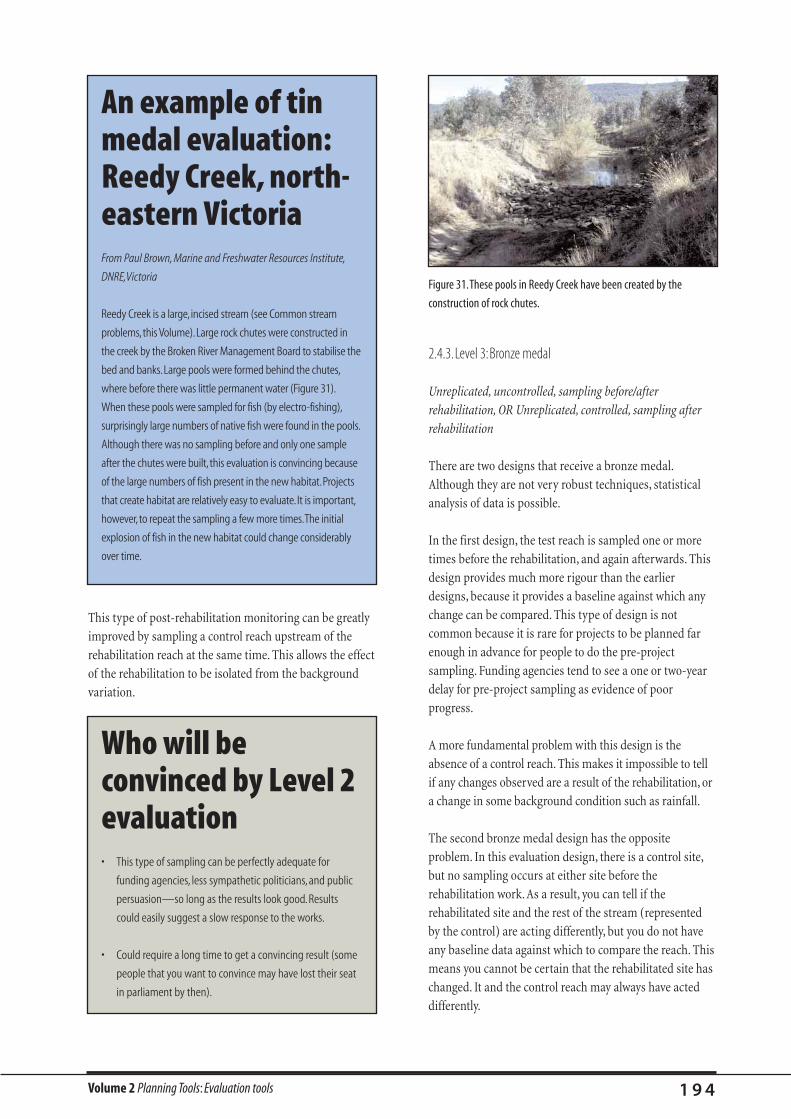
Volume 2 Planning Tools: Evaluation tools 1 9 4
This type of post-rehabilitation monitoring can be greatly
improved by sampling a control reach upstream of the
rehabilitation reach at the same time. This allows the effect
of the rehabilitation to be isolated from the background
variation.
2.4.3.Level 3:Bronze medal
Unreplicated, uncontrolled, sampling before/after
rehabilitation, OR Unreplicated, controlled, sampling after
rehabilitation
There are two designs that receive a bronze medal.
Although they are not very robust techniques, statistical
analysis of data is possible.
In the first design, the test reach is sampled one or more
times before the rehabilitation, and again afterwards. This
design provides much more rigour than the earlier
designs, because it provides a baseline against which any
change can be compared. This type of design is not
common because it is rare for projects to be planned far
enough in advance for people to do the pre-project
sampling. Funding agencies tend to see a one or two-year
delay for pre-project sampling as evidence of poor
progress.
A more fundamental problem with this design is the
absence of a control reach. This makes it impossible to tell
if any changes observed are a result of the rehabilitation, or
a change in some background condition such as rainfall.
The second bronze medal design has the opposite
problem. In this evaluation design, there is a control site,
but no sampling occurs at either site before the
rehabilitation work. As a result, you can tell if the
rehabilitated site and the rest of the stream (represented
by the control) are acting differently, but you do not have
any baseline data against which to compare the reach. This
means you cannot be certain that the rehabilitated site has
changed. It and the control reach may always have acted
differently.
An example of tinmedal evaluation:Reedy Creek, north-eastern Victoria From Paul Brown, Marine and Freshwater Resources Institute,
DNRE,Victoria
Reedy Creek is a large, incised stream (see Common stream
problems,this Volume).Large rock chutes were constructed in
the creek by the Broken River Management Board to stabilise the
bed and banks.Large pools were formed behind the chutes,
where before there was little permanent water (Figure 31).
When these pools were sampled for fish (by electro-fishing),
surprisingly large numbers of native fish were found in the pools.
Although there was no sampling before and only one sample
after the chutes were built, this evaluation is convincing because
of the large numbers of fish present in the new habitat.Projects
that create habitat are relatively easy to evaluate. It is important,
however, to repeat the sampling a few more times.The initial
explosion of fish in the new habitat could change considerably
over time.
Figure 31.These pools in Reedy Creek have been created by the
construction of rock chutes.
Who will beconvinced by Level 2evaluation • This type of sampling can be perfectly adequate for
funding agencies, less sympathetic politicians, and public
persuasion—so long as the results look good. Results
could easily suggest a slow response to the works.
• Could require a long time to get a convincing result (some
people that you want to convince may have lost their seat
in parliament by then).
Volume 2 Planning Tools: Evaluation tools 1 9 5
2.4.4.Level 4:Silver medal
Unreplicated, controlled, sampling before/after intervention
This is the standard BACI design
(before–after–control–intervention) for experiments
(Green, 1979). Both the target reach and an independent
control reach are sampled before and after the
rehabilitation. In this way the relationship between the
control and the rehabilitation site is established before the
rehabilitation begins. Any new differences between the
control and the target sites after the rehabilitation can then
be assumed to be caused by that intervention. There will
usually be a statistical analysis of the data.
2.4.5.Level 5:Gold medal
Replicated sampling, replicated controls, before–after
intervention
This is the ‘Beyond BACI’ design (see Underwood, 1996),
the most robust evaluation available for most stream
rehabilitation. Statistical analysis of the data will almost
always be a part of this design. The replicated sampling
means differences before and after rehabilitation can be
detected with more accuracy, and the use of multiple
control reaches means the changes can be attributed to the
rehabilitation with greater confidence. If your
rehabilitation project involves treating several reaches of
stream, incorporating all of these into the evaluation will
also increase the confidence in the results. If the control
and rehabilitation sites cover more than one stream, the
results will be more widely applicable. Unfortunately, this
design, while being the most robust against all criticism,
tends to be so expensive that it is seldom used.
Who will be convinced by Level 3evaluation • Usually adequate for publication in trade journals like
Landcare magazines etc.
• This is the level of confidence that would convince a
sceptical senior manager, but would generate debate (but
not necessarily complete rejection) amongst scientists
about the ‘validity of the experimental design’. (Will be
better received if there is both replication and a control in
the design.)
Who will beconvinced by Level 4evaluation ? • Standard BACI design evaluation would easily convince a
sceptical senior manager,
• A replicated BACI design (ie. several samples taken at each
site) is considered the minimum standard for most journal
publications.
Who will beconvinced by Level 5evaluation ? • The result would be difficult to argue with once the study
is completed, and would provide strong grounds for
management decisions.
• This is the level of confidence that is usually required for
publication in an international scientific journal.
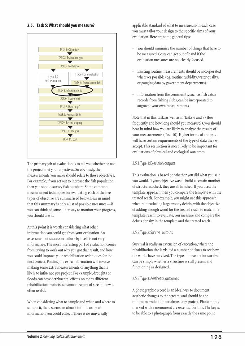
Volume 2 Planning Tools: Evaluation tools 1 9 6
2.5. Task 5: What should you measure?
The primary job of evaluation is to tell you whether or not
the project met your objectives. So obviously, the
measurements you make should relate to those objectives.
For example, if you set out to increase the fish population,
then you should survey fish numbers. Some common
measurement techniques for evaluating each of the five
types of objective are summarised below. Bear in mind
that this summary is only a list of possible measures—if
you can think of some other way to monitor your progress,
you should use it.
At this point it is worth considering what other
information you could get from your evaluation. An
assessment of success or failure by itself is not very
informative. The most interesting part of evaluation comes
from trying to work out why you got that result, and how
you could improve your rehabilitation techniques for the
next project. Finding the extra information will involve
making some extra measurements of anything that is
likely to influence you project. For example, droughts or
floods can have detrimental effects on many different
rehabilitation projects, so some measure of stream flow is
often useful.
When considering what to sample and when and where to
sample it, there seems an almost infinite array of
information you could collect. There is no universally
applicable standard of what to measure, so in each case
you must tailor your design to the specific aims of your
evaluation. Here are some general tips:
• You should minimise the number of things that have to
be measured. Costs can get out of hand if the
evaluation measures are not clearly focused.
• Existing routine measurements should be incorporated
wherever possible (eg. routine turbidity, water quality,
or gauging data by government departments).
• Information from the community, such as fish catch
records from fishing clubs, can be incorporated to
augment your own measurements.
Note that in this task, as well as in Tasks 6 and 7 (How
frequently and how long should you measure?), you should
bear in mind how you are likely to analyse the results of
your measurements (Task 10). Higher forms of analysis
will have certain requirements of the type of data they will
accept. This restriction is most likely to be important for
evaluations of physical and ecological outcomes.
2.5.1.Type 1:Execution outputs
This evaluation is based on whether you did what you said
you would. If your objective was to build a certain number
of structures, check they are all finished. If you used the
template approach then you compare the template with the
treated reach. For example, you might use this approach
when reintroducing large woody debris, with the objective
of adding enough wood for the treated reach to match the
template reach. To evaluate, you measure and compare the
debris density in the template and the treated reach.
2.5.2.Type 2:Survival outputs
Survival is really an extension of execution, where the
rehabilitation site is visited a number of times to see how
the works have survived. The type of measure for survival
can be simply whether a structure is still present and
functioning as designed.
2.5.3.Type 3:Aesthetics outcomes
A photographic record is an ideal way to document
aesthetic changes to the stream, and should be the
minimum evaluation for almost any project. Photo points
marked with a monument are essential for this. The key is
to be able to a photograph from exactly the same point
TASK 1: Objectives
TASK 2: Evaluation type
TASK 3: Confidence
TASK 11: Cost
TASK 5: Measurements
TASK 6: How often?
TASK 7: How long?
TASK 8: Responsibility
TASK 9: Record keeping
TASK 10: Analysis
TASK 4: Evaluation medals
If type 4 or 5 evaluationIf type 1,2
or 3 evaluation
Volume 2 Planning Tools: Evaluation tools 1 9 7
each time the site is visited. This is accomplished simply
using any of the following strategies.
• Several large nails hammered into a large log.You slide
the camera into the space between the nails and it is held
fast so that a consistent photo can be taken each time.
• Custom designed photo-point made from a wooden
pole cemented into the ground.
• Three cement plugs (or similar) buried in the ground,
on which to place a camera tripod.
2.5.4 Type 4:Physical and chemical outcomes
The long-term goal of stream rehabilitation is usually to
increase the ecological diversity of the stream. However,
physical habitat is easier to measure that stream
ecology—it doesn’t try to bite or run away, and it’s not
difficult to identify.You are then left with the assumption
that if the physical change has occurred, then the desired
ecological changes will follow. But what exactly do you
measure?
• Channel morphology, bed sediments and large woody
debris are structural features which influence the
hydraulic environment.
• Flow types and patterns of depth, velocity and shear
stress characterise the hydraulic environment.
• Water quality parameters, such as turbidity,
temperature, salinity, and so on.
The Little Butte Creek evaluation, summarised in Table 27,
is a good example of the sorts of physical measurements
you can take.
When designing a project based on the physical habitat,
you have to be careful to remember the animals and plants
you are attempting to encourage. The objectives of your
project should reflect the needs of those organisms (this
can be tricky if the needs of the organisms are not well
known). This section briefly outlines some methods for
describing the structural character of stream channels.
Surveying
Many measures of physical changes in the stream are
based on repeated surveys, usually either of cross-sections
or long profiles. The key to useful surveying is to include a
benchmark—something that is not going to move, like a
tree or fencepost. This means that you can compare
surveys from before and after rehabilitation. The
benchmark helps you position later surveys in exactly the
same spot, and also makes it easier to compare the results.
Channel morphology
Commonly measured features of channel morphology are:
• average depth;
• how depth varies (eg. an area of shallow, uniform flow,
might change after rehabilitation into a sequence of
deep pools and shallow riffles);
• the presence or absence of particular features of the
channel, such as undercuts, or bars; and
• the shape of the channel (eg. bank height or slope, or
channel width).
There are statistical techniques available to characterise
the variation revealed by such surveys (eg. see Western
et al., in press).
Sediment characteristics
Particle size is the most commonly measured
characteristic of the sediment.
Large woody debris
In streams with only small quantities of large woody
debris, measurement is a simple matter of counting the
pieces, and perhaps noting the size and type. In streams
that are more densely laden with debris, the easiest
method of measuring abundance is the line intercept
method (Gippel et al., 1996a).
Flow types
Flow types (ie. pools, riffles, runs and so on) can be
characterised by simply counting the number and
abundance of different types, or by measuring the area of
each type. Rowntree and Wadeson (1996) present clear
definitions of 11 different flow types, and a statistical
technique to characterise the complexity of flow types
in a reach.
Volume 2 Planning Tools: Evaluation tools 1 9 8
On a far smaller scale, it is possible to measure hydraulic
micro-habitat, characterised by velocity and depth, and
thus calculate the hydraulic diversity for the reach
(Stewardson et al., 1999).
Habitat
Often when monitoring a stream you end up with a very
large and complex collection of data. It is very useful to be
able to reduce these to a single number, which means you
have a chance of interpreting your results. The ‘weighted
useable area’ model (developed in the USA) is a good
method of assessing the availability of habitat for
individual species or life stages (Nestler et al., 1989).
Water quality
Some projects will have as their objective an improvement
in water quality. Commonly used water quality parameters
are discussed in Common stream problems, this Volume.
2.5.5.Type 5:Ecological outcomes
The core of ecological outcomes is the identification of
plants or animals to an appropriate taxonomic level,
whether that be family, genus or species. Depending on the
level of identification, and the organisms involved, this can
require considerable expertise. Obviously, plants are the
easiest to survey (they’re not too hard to catch!). The larger
algae are also easy to sample, but identification requires a
microscope and considerable expertise. Macroinvertebrates
can be collected using fine nets (Tiller and Metzeling,
1998). Fact sheets such as those produced for Streamwatch
(eg. Sydney Water and CSIRO) will help in identifying the
more common orders of animal (eg. dragonfly, leech,
beetle), but more detailed identification will require an
expert. Fish can also be captured using nets (although this
risks injuring or killing some individuals) or using electro-
fishing. Note that identification of juvenile fish is very
difficult. Platypus, birds and frogs can be surveyed by
careful observations at appropriate times of day.
Having identified the relevant organisms, you can:
• measure the diversity and abundance of different
taxonomic groups (eg. has the proportion of species
that indicate a healthy stream increased?);
• look for the presence of different life stages (eg. now we
have fenced stock out of the riparian zone, is there any
natural regeneration of the riparian species?). Note that
identification of juvenile organisms can be very
difficult; or
• look for differences in the behaviour of animals (eg. are
the fish found around the new habitat we
constructed?).
There is a range of tools available to help you make sense
from what can be a large and complex data set. These tools
include measures of diversity, such as EPT scores, through
to models based on empirical data, such as AusRivAS, and
complex statistical analysis, such as multi-dimensional
scaling. These techniques are discussed in Using Bio-
indicators, in Catchment review, this volume.
2.5.6.Other information you may need to collect
As suggested in the introduction to this task, a good
evaluation will tell you not only if your project succeeded
or failed, but also what factors contributed to that result,
and how your techniques could be improved for your next
project. In order to extract such fascinating tips from your
evaluation, you will need to feed in some extra information
about things that are likely to influence the outcome of the
project.
It is often good to incorporate measurement techniques
from lower evaluation types into your monitoring
program. For example, a Type 5 ecological evaluation could
also incorporate records of physical features, records of
how structures have survived, whether they were executed
properly and use photo-point surveys. These types of
information will allow you to track the development of the
project. It is unlikely that the ecological outcomes will
occur if, for some reason, the works are not completed as
planned, or they are damaged by a flood, or the physical
outcomes sought do not develop.
You should also collect data relating to the general
condition of the stream and catchment. For example, it is
almost always useful to have some measure of discharge
through the project reach. This may be provided by a
nearby gauge, or it can be estimated from a gauge in a
nearby catchment. Discharge data will tell you all sorts of
things about what is driving the changes in your reach.You
may get a general deepening of the channel in your reach,
but this could be related to an unusually long period of
winter flow rather than a result of any structures you have
built. Such catchment-wide changes should be identified

Volume 2 Planning Tools: Evaluation tools 1 9 9
by comparing your site with a control, but having a
discharge measurement will allow you to explain the change
as well as observe it. Other things you may measure
regularly could be aspects of water quality such as turbidity,
nutrients, temperature, dissolved oxygen, or salinity.
Similarly, having a general feel for changes in the
catchment could also help in interpretation. For example,
the changes you observe could be explained by long
sections of stream being cleared upstream, or a reduction
in nutrient-rich wastewater from piggeries upstream.
Perhaps the changes you find at your site could be
explained by these catchment-scale changes, and not by
the local changes that you are introducing.
2.6. Task 6: How frequently should you monitor?
combination of event and predetermined frequency will
usually be the most effective strategy (Kondolf, 1995).
Table 29 shows some common rehabilitation activities, the
measurable objective and suggested frequencies and
duration of sampling. Table 30 shows a summary of
evaluation projects, their key measure and the frequency
and duration of sampling.
2.6.1.Event-based sampling
Kondolf (1995) recommends a monitoring period of 10
years to successfully evaluate a project. Measurements
need not be made every year, but there should be a series
of at least 5 monitoring events over the 10-year period.
Monitoring is conducted in, say, years 1, 2, 4, 7, and 10, or
following each flow exceeding some threshold such as the
annual peak flow, with return periods of 2 or 5 years
(Kondolf, 1995). Therefore, if a flood occurred in year 6 the
stream would be surveyed and not again until year 10
(unless the predetermined flow was again exceeded). This
sampling program is good for projects concerned with
stream stability, which are affected by flow size.
2.6.2.Sampling at a predetermined frequency
There are two questions to ask yourself about sampling at
a predetermined frequency. First, what time of year are you
interested in sampling, and second, do you need to sample
every year?
The answer to the first question depends on what your
interests are. For example, if you have decided to monitor
how stream animals are responding to rehabilitation, you
should consider whether you are interested in the summer
or winter fauna, or both. Particularly for
macroinvertebrates, you are likely to find quite different
suites of species present in different seasons. If you want to
survey the riparian vegetation, you may find spring is the
best season, because plants are easier to identify when
they are flowering. If you are monitoring water quality, you
may find the summer base-flow differs markedly from
winter flows, when some pollutants (such as salt) are
diluted by extra flow, while the concentration of others
(such as suspended sediment) will increase. Anything that
varies seasonally should always be measured at the same
time of year. If, for example, you surveyed invertebrates in
winter, just before your rehabilitation work, and then in
summer, after the work, you could not be sure which
differences were caused by your actions, and which were
natural seasonal variation.
TASK 1: Objectives
TASK 2: Evaluation type
TASK 3: Confidence
TASK 11: Cost
TASK 5: Measurements
TASK 6: How often?
TASK 7: How long?
TASK 8: Responsibility
TASK 9: Record keeping
TASK 10: Analysis
TASK 4: Evaluation medals
If type 4 or 5 evaluationIf type 1,2
or 3 evaluation
There are two basic strategies for deciding on sampling
frequency: event-based sampling, and sampling at a
predetermined frequency. Event-based sampling is
particularly relevant for structural works in a stream when
we want to observe the effect of our intervention after
floods greater than a set magnitude. Predetermined
sampling frequency is where the sampling times are
specified at the design stage and are not linked to flood
events. Depending on what you are measuring, a
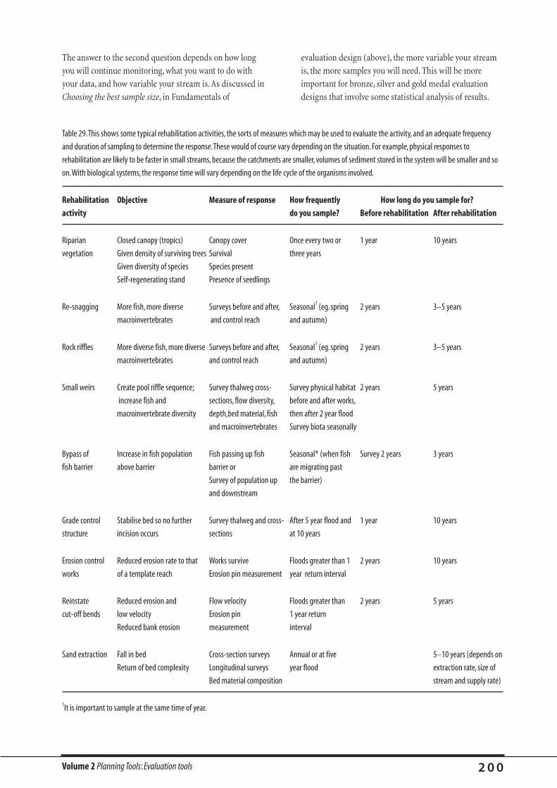
Volume 2 Planning Tools: Evaluation tools 2 0 0
The answer to the second question depends on how long
you will continue monitoring, what you want to do with
your data, and how variable your stream is. As discussed in
Choosing the best sample size, in Fundamentals of
evaluation design (above), the more variable your stream
is, the more samples you will need. This will be more
important for bronze, silver and gold medal evaluation
designs that involve some statistical analysis of results.
Table 29.This shows some typical rehabilitation activities, the sorts of measures which may be used to evaluate the activity, and an adequate frequency
and duration of sampling to determine the response.These would of course vary depending on the situation. For example, physical responses to
rehabilitation are likely to be faster in small streams, because the catchments are smaller, volumes of sediment stored in the system will be smaller and so
on.With biological systems, the response time will vary depending on the life cycle of the organisms involved.
Rehabilitation Objective Measure of response How frequently How long do you sample for?
activity do you sample? Before rehabilitation After rehabilitation
Riparian Closed canopy (tropics) Canopy cover Once every two or 1 year 10 years
vegetation Given density of surviving trees Survival three years
Given diversity of species Species present
Self-regenerating stand Presence of seedlings
Re-snagging More fish, more diverse Surveys before and after, Seasonal1 (eg. spring 2 years 3–5 years
macroinvertebrates and control reach and autumn)
Rock riffles More diverse fish, more diverse Surveys before and after, Seasonal1 (eg. spring 2 years 3–5 years
macroinvertebrates and control reach and autumn)
Small weirs Create pool riffle sequence; Survey thalweg cross- Survey physical habitat 2 years 5 years
increase fish and sections, flow diversity, before and after works,
macroinvertebrate diversity depth,bed material, fish then after 2 year flood
and macroinvertebrates Survey biota seasonally
Bypass of Increase in fish population Fish passing up fish Seasonal* (when fish Survey 2 years 3 years
fish barrier above barrier barrier or are migrating past
Survey of population up the barrier)
and downstream
Grade control Stabilise bed so no further Survey thalweg and cross- After 5 year flood and 1 year 10 years
structure incision occurs sections at 10 years
Erosion control Reduced erosion rate to that Works survive Floods greater than 1 2 years 10 years
works of a template reach Erosion pin measurement year return interval
Reinstate Reduced erosion and Flow velocity Floods greater than 2 years 5 years
cut-off bends low velocity Erosion pin 1 year return
Reduced bank erosion measurement interval
Sand extraction Fall in bed Cross-section surveys Annual or at five 5–10 years (depends on
Return of bed complexity Longitudinal surveys year flood extraction rate, size of
Bed material composition stream and supply rate)
1It is important to sample at the same time of year.

Volume 2 Planning Tools: Evaluation tools 2 0 1
Table 30.This table shows the duration and frequency of sampling from some evaluations made of rehabilitation projects (mostly from the USA).
Study Measure Frequency Duration
Before rehabilitation After rehabilitation
Koehn (1987) Fish surveys Once before, once after 2 months 3 years
rehabilitation
Newbury and Trout eggs Annual None 6 years
Gaboury (1993)
Mallen-Cooper Fish numbers passing Annual 2 years 2 years
et al. (1995)
Shields et al. Bed and bank stability Variable None Variable. Up to 10 years
(1995a) Cover of vegetation monitoring, with up to
8 years casual
observations after that
Shields et al. (1995c) Fish species composition and abundance Twice yearly 2 years 1 year
Physical habitat (pool area, heterogeneity,
riparian vegetation, shade, woody debris)
Frissell and Nawa Condition of stream structures After a 2–10 year flood None Once
(1992)
House and Boehne Stability of structures Annual Shortly before 2 years
(1985) Channel morphology rehabilitation
Fish utilisation of habitat
Juvenile fish density and biomass
House (1996) Habitat diversity Habitat was measured in 1 year 11 years
Juvenile fish populations year 1, 3 and 5
Spawning sites Other measures taken
Gravel quality annually
Hunt (1976) Number and size distribution of trout
Trout biomass Annually 3 years 7 years
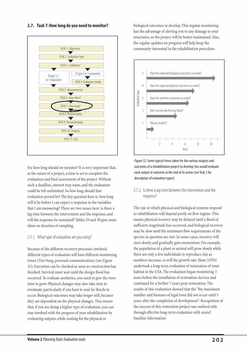
Volume 2 Planning Tools: Evaluation tools 2 0 2
2.7. Task 7: How long do you need to monitor? biological outcomes to develop. This regular monitoring
has the advantage of alerting you to any damage to your
structures, so the project will be better maintained. Also,
the regular updates on progress will help keep the
community interested in the rehabilitation procedure.
Figure 32. Some typical times taken for the various outputs and
outcomes of a rehabilitation project to develop.You would evaluate
each output or outcome at the end of its arrow (see Task 2 for
description of evaluation types).
5 Have the expected biological outcomes occurred?
4 Have the expected physical outcomes occurred?
3 Have the aesthetic outcomes occurred?
2 Did it survive the first big flood?
1 Did you build it?
2 4 6 8 10
Years
Evalu
ation
type
TASK 1: Objectives
TASK 2: Evaluation type
TASK 3: Confidence
TASK 11: Cost
TASK 5: Measurements
TASK 6: How often?
TASK 7: How long?
TASK 8: Responsibility
TASK 9: Record keeping
TASK 10: Analysis
TASK 4: Evaluation medals
If type 4 or 5 evaluationIf type 1,2
or 3 evaluation
For how long should we monitor? It is very important that,
at the outset of a project, a time is set to complete the
evaluation and final assessment of the project. Without
such a deadline, interest may wane, and the evaluation
could be left unfinished. So how long should that
evaluation period be? The key question here is: how long
will it be before I can expect a response in the variables
that I am measuring? There are two issues here: is there a
lag time between the intervention and the response, and
will the response be sustained? Tables 29 and 30 give some
ideas on duration of sampling.
2.7.1. What type of evaluation are you using?
Because of the different recovery processes involved,
different types of evaluation will have different monitoring
times (Tim Doeg, personal communication) (see Figure
32). Execution can be checked as soon as construction has
finished. Survival must wait until the design flood has
occurred. To evaluate aesthetics, you need to give the trees
time to grow. Physical changes may also take time to
eventuate, particularly if you have to wait for floods to
occur. Biological outcomes may take longer still, because
they are dependent on the physical changes. This means
that, if you are doing a higher type of evaluation, you can
stay involved with the progress of your rehabilitation by
evaluating outputs, while waiting for the physical or
2.7.2. Is there a lag time between the intervention and theresponse?
The rate at which physical and biological systems respond
to rehabilitation will depend partly on flow regime. This
means physical recovery may be delayed until a flood of
sufficient magnitude has occurred, and biological recovery
may be slow until the minimum flow requirements of the
species in question are met. In some cases, recovery will
start slowly, and gradually gain momentum. For example,
the population of a plant or animal will grow slowly while
there are only a few individuals to reproduce, but as
numbers increase, so will the growth rate. Hunt (1976)
undertook a long-term evaluation of restoration of trout
habitat in the USA. The evaluation began monitoring 3
years before the installation of restoration devices and
continued for a further 7 years post-restoration. The
results of this evaluation showed that the "the maximum
number and biomass of legal trout did not occur until 5
years after the completion of development". Recognition of
the success of this restoration project was realised only
through effective long-term evaluation with sound
baseline information.
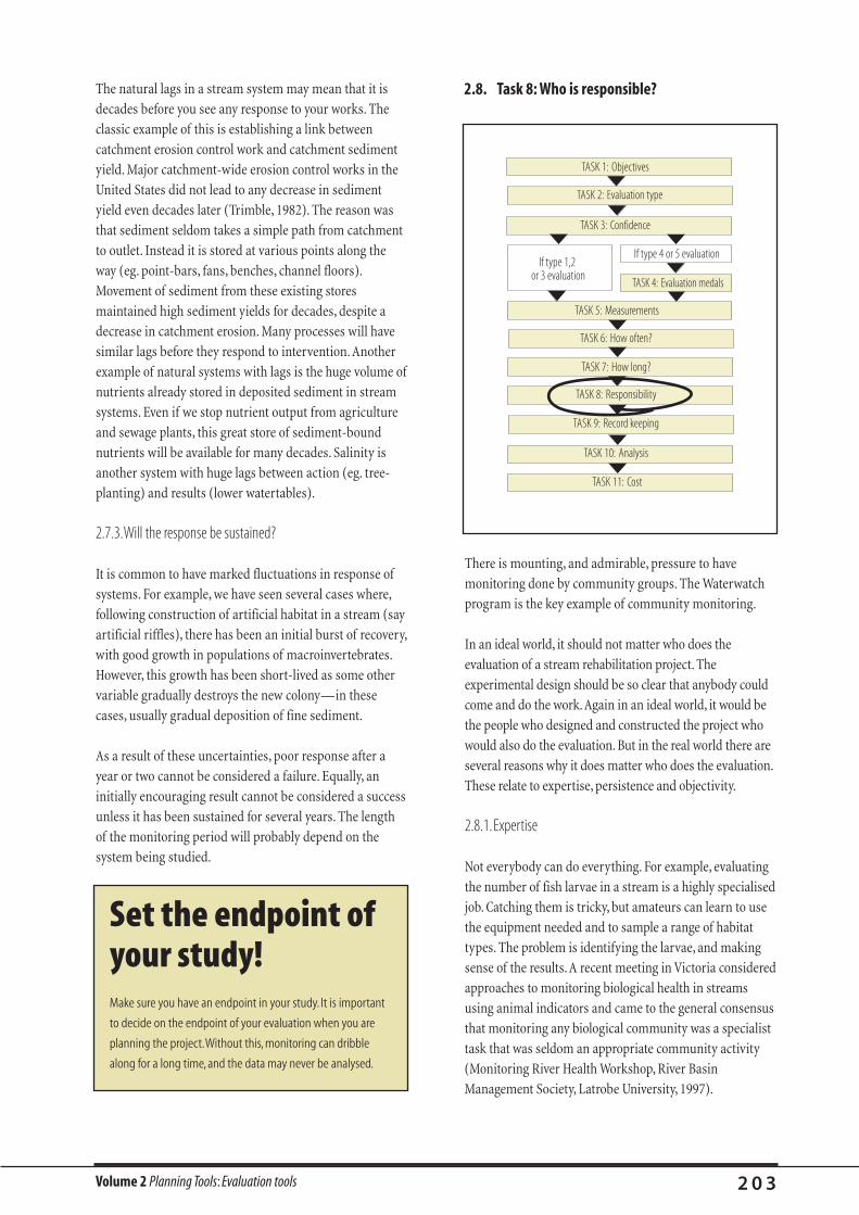
Volume 2 Planning Tools: Evaluation tools 2 0 3
The natural lags in a stream system may mean that it is
decades before you see any response to your works. The
classic example of this is establishing a link between
catchment erosion control work and catchment sediment
yield. Major catchment-wide erosion control works in the
United States did not lead to any decrease in sediment
yield even decades later (Trimble, 1982). The reason was
that sediment seldom takes a simple path from catchment
to outlet. Instead it is stored at various points along the
way (eg. point-bars, fans, benches, channel floors).
Movement of sediment from these existing stores
maintained high sediment yields for decades, despite a
decrease in catchment erosion. Many processes will have
similar lags before they respond to intervention. Another
example of natural systems with lags is the huge volume of
nutrients already stored in deposited sediment in stream
systems. Even if we stop nutrient output from agriculture
and sewage plants, this great store of sediment-bound
nutrients will be available for many decades. Salinity is
another system with huge lags between action (eg. tree-
planting) and results (lower watertables).
2.7.3.Will the response be sustained?
It is common to have marked fluctuations in response of
systems. For example, we have seen several cases where,
following construction of artificial habitat in a stream (say
artificial riffles), there has been an initial burst of recovery,
with good growth in populations of macroinvertebrates.
However, this growth has been short-lived as some other
variable gradually destroys the new colony—in these
cases, usually gradual deposition of fine sediment.
As a result of these uncertainties, poor response after a
year or two cannot be considered a failure. Equally, an
initially encouraging result cannot be considered a success
unless it has been sustained for several years. The length
of the monitoring period will probably depend on the
system being studied.
2.8. Task 8: Who is responsible?
TASK 1: Objectives
TASK 2: Evaluation type
TASK 3: Confidence
TASK 11: Cost
TASK 5: Measurements
TASK 6: How often?
TASK 7: How long?
TASK 8: Responsibility
TASK 9: Record keeping
TASK 10: Analysis
TASK 4: Evaluation medals
If type 4 or 5 evaluationIf type 1,2
or 3 evaluation
Set the endpoint ofyour study!Make sure you have an endpoint in your study. It is important
to decide on the endpoint of your evaluation when you are
planning the project.Without this, monitoring can dribble
along for a long time, and the data may never be analysed.
There is mounting, and admirable, pressure to have
monitoring done by community groups. The Waterwatch
program is the key example of community monitoring.
In an ideal world, it should not matter who does the
evaluation of a stream rehabilitation project. The
experimental design should be so clear that anybody could
come and do the work.Again in an ideal world, it would be
the people who designed and constructed the project who
would also do the evaluation. But in the real world there are
several reasons why it does matter who does the evaluation.
These relate to expertise, persistence and objectivity.
2.8.1.Expertise
Not everybody can do everything. For example, evaluating
the number of fish larvae in a stream is a highly specialised
job. Catching them is tricky, but amateurs can learn to use
the equipment needed and to sample a range of habitat
types. The problem is identifying the larvae, and making
sense of the results.A recent meeting in Victoria considered
approaches to monitoring biological health in streams
using animal indicators and came to the general consensus
that monitoring any biological community was a specialist
task that was seldom an appropriate community activity
(Monitoring River Health Workshop, River Basin
Management Society, Latrobe University, 1997).
Volume 2 Planning Tools: Evaluation tools 2 0 4
This, of course, has been the perennial argument with the
Waterwatch program, in which members of the
community monitor water quality. The consensus here is
that the data provide useful descriptive information over a
large area, and that the process is useful for raising
awareness and for uncovering local problems missed by
other monitoring, but the value of the data in scientific
and management terms is limited (Hodgkins and
Bennison, 1997). Again, it comes back to confidence. Gold
medal monitoring produces data that are consistently
accurate, and can be compared confidently with samples
taken, say, 3 years ago by somebody else from another site
100 km away. It is important to consider whether your
particular evaluation requires this level of confidence.
Even some of the most basic of monitoring techniques
cannot readily be used by community groups because of
the specialised equipment and expertise required. For
example, electro-fishing, which is the most common
method of field-sampling for fish, can be done only by
highly qualified people.
2.8.2.Persistence
Detailed monitoring is often a boring, repetitive activity.
Techniques have to be applied with ruthless consistency,
and you have to go out whatever the weather, or however
you feel. Monitoring has to continue even when nothing
seems to be happening, or when the results are not what
you wanted. And it often has to continue for years.
It is rare to find volunteers who have the stamina and
persistence to face the rigours of a long-term monitoring
program. However, if the monitoring involves simple
protocols (eg. repeat photographs, counting something
that is easy to count, identifying the presence or absence of
something) then community members will be ideal for the
job. Nevertheless, one person has to maintain
responsibility for the quality of the data.
2.8.3.Objectivity
The foundation of evaluation is objectivity. Workers should
measure and report bad news equally with good news. The
ethic of scientists is to seek truth and to ensure that their
own prejudices do not affect the ‘outcome’ of an
experiment (this ethic is ‘policed’ by the critical review of
scientific colleagues). Evaluation by people who are
desperate for a particular outcome (ie. success) is less
likely to be entirely objective. This is not even a question of
honesty; rather it is the fact that people tend to see and
measure what they want to see and measure, rather than
what is true. If you don’t believe that, consider how many
people believe that their babies are the most beautiful
babies ever born. Thus, for reasons of objectivity, it is best
to have a project evaluated by people other than those who
initiated it.
On the other hand, there are strong arguments for
evaluation to be done by the same people who proposed,
planned and executed the project. This has the best
learning outcomes. Perhaps a middle ground is best, with
monitoring done by the proponents of the project, while
the methods and quality of the monitoring are evaluated
by scientists.
2.8.4.Conclusions on responsibility
Most long-term monitoring will be carried out by
professional scientists. There are many types of monitoring
that can be done by non-professionals, but one person has
to be responsible for the continuity and quality of the data.
Whoever does the evaluation, a critically important point
is that the protocol and procedures for monitoring are so
well documented that a new person can come in and
reproduce the procedure. This is essential given the high
turnover of personnel that is likely over a monitoring
project that could last 5–10 years. For the same reason, the
locations of all cross-sections and other measurement
points should be clearly recorded and on-site ‘monuments’
installed. There are numerous examples of evaluation
projects foundering because it was so difficult for new staff
to work out what had been done, and where. Harrelson et
al. (1994) give a detailed discussion of how to prepare and
monument cross-sections, and generally plan rigorous
field work.
"Whilst enthusiasm and energy are important assets to
community involvement in environmental monitoring
programs, in the long-run it will be data quality and reliability
which will be the defining criteria of success" (Hodgkins and
Bennison, 1997, p.9).
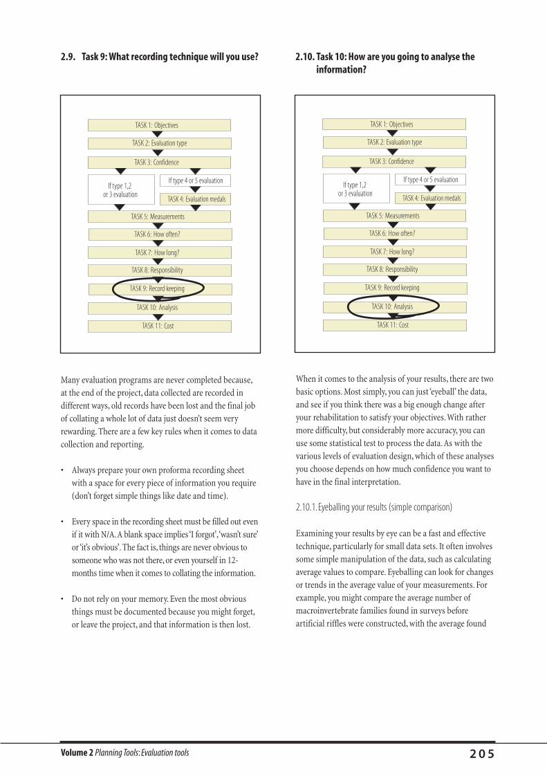
Volume 2 Planning Tools: Evaluation tools 2 0 5
2.9. Task 9: What recording technique will you use? 2.10. Task 10: How are you going to analyse theinformation?
TASK 1: Objectives
TASK 2: Evaluation type
TASK 3: Confidence
TASK 11: Cost
TASK 5: Measurements
TASK 6: How often?
TASK 7: How long?
TASK 8: Responsibility
TASK 9: Record keeping
TASK 10: Analysis
TASK 4: Evaluation medals
If type 4 or 5 evaluationIf type 1,2
or 3 evaluation
TASK 1: Objectives
TASK 2: Evaluation type
TASK 3: Confidence
TASK 11: Cost
TASK 5: Measurements
TASK 6: How often?
TASK 7: How long?
TASK 8: Responsibility
TASK 9: Record keeping
TASK 10: Analysis
TASK 4: Evaluation medals
If type 4 or 5 evaluationIf type 1,2
or 3 evaluation
Many evaluation programs are never completed because,
at the end of the project, data collected are recorded in
different ways, old records have been lost and the final job
of collating a whole lot of data just doesn’t seem very
rewarding. There are a few key rules when it comes to data
collection and reporting.
• Always prepare your own proforma recording sheet
with a space for every piece of information you require
(don’t forget simple things like date and time).
• Every space in the recording sheet must be filled out even
if it with N/A.A blank space implies ‘I forgot’,‘wasn’t sure’
or ‘it’s obvious’. The fact is, things are never obvious to
someone who was not there, or even yourself in 12-
months time when it comes to collating the information.
• Do not rely on your memory. Even the most obvious
things must be documented because you might forget,
or leave the project, and that information is then lost.
When it comes to the analysis of your results, there are two
basic options. Most simply, you can just ‘eyeball’ the data,
and see if you think there was a big enough change after
your rehabilitation to satisfy your objectives. With rather
more difficulty, but considerably more accuracy, you can
use some statistical test to process the data. As with the
various levels of evaluation design, which of these analyses
you choose depends on how much confidence you want to
have in the final interpretation.
2.10.1.Eyeballing your results (simple comparison)
Examining your results by eye can be a fast and effective
technique, particularly for small data sets. It often involves
some simple manipulation of the data, such as calculating
average values to compare. Eyeballing can look for changes
or trends in the average value of your measurements. For
example, you might compare the average number of
macroinvertebrate families found in surveys before
artificial riffles were constructed, with the average found

Volume 2 Planning Tools: Evaluation tools 2 0 6
after construction. It can be as simple as comparing two
numbers. For example, you surveyed the fish population of
the reach once before and once after constructing the
riffles, and found five times more fish in the second survey.
Alternatively, you can look for patterns of change. For
example, you might compare the long profiles of the reach
before the riffles were constructed, with the profile straight
after construction, and after a one-in-three-year flood.You
would be looking for the riffles to be shallower, and the
pools between riffles to become deeper.
Eyeballing results is usually quick, easy and intuitive, and
can be convincing when the rehabilitation caused a big
change in the stream. However, it does not suit all data, or
all purposes. It is difficult to be truly objective.You put a lot
of effort into your rehabilitation project, and the stream
looks so much better with those riffles and the pools below
them. It is very difficult not to let your hopes and the belief
you have improved conditions colour your judgment,
however hard you try to prevent this.Also, large and
complex data sets can be almost impossible to comprehend
without mathematical help. How do you cope with lots of
individual data points, all of which seem to vary in
different ways? For example, if you survey
macroinvertebrates in a relatively healthy stream, you could
quite easily find over 50 different species. How do you make
sense of your results when, after rehabilitation, some have
increased abundance, others have decreased, there are
some new species and others have disappeared. However,
the greatest shortcoming of eyeballing data is its inability
to take into account the variation in natural systems.
Eyeballing can be very useful, but because of the difficulty
of taking variation into account, this sort of analysis is
really convincing only when the change caused by the
rehabilitation project is dramatically large. No-one is going
to argue you made a difference if you catch 10 times more
fish than before, but what if you only catch a few more,
like Joe in the example that follows?
A hypotheticalexample ofanalysing theresults of anevaluationJoe the stream manager had constructed some rather
expensive artificial riffles in a reach that had several shallow
headcuts.The channel had no deep pools and had a small fish
population. Joe had wanted to do a first-class evaluation to
show how well the riffles worked. He had fish survey data for
four years before the riffles were constructed, and he surveyed
for another four years after construction. At the end of the
evaluation, Joe sat down and looked at the surveyed results
(Table 31).Though they were not as dramatic as he’d hoped, he
felt confident that there had been a moderate increase in the
fish population. Pleased, Joe showed the results to his mate,
Chris the ecologist, who he ran into on his way to apply for
more money to build more riffles.
Table 31.The number of fish Joe found before and after the
riffles were built.
Before 11 28 13 24 Average 19
After 17 24 19 36 Average 24
Chris looked at the results, and shook his head."Well, we’ll leave
out the lack of a control site", he said. "These numbers may
actually show the fish population hasn’t changed at all.
Remember that when you sample, you are not really measuring
the population of fish, just how many you happen to catch in
that survey.Some days you get lucky, and even though the fish
population is the same, you catch more fish. See, before you
even put in the riffles, your fish counts varied between 28 and
11. As well as that, natural populations are always changing a
bit. If you look at how much variation there is in your results, I’d
say there’s a fair chance you didn’t really change the total fish
population at all, and you just got higher results in the second
survey by chance." Chris did a few simple statistical tests called
t-tests.These showed that in fact Joe couldn’t be sure that the
fish population has really increased, but there was a 78%
chance that it had."Well", said Chris, "it wouldn’t convince
everybody.Usually, scientists would only say fish numbers had
changed if they could be 95% certain. I suppose you have to
consider how certain of success you want to be, before you
spend all that money building more riffles!"
Eyeballing is:
• quick, easy and cheap;
• only trustworthy for detecting big changes;
• only good for small data sets;
• subjective; and
• will not convince sceptics.
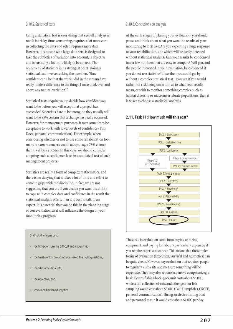
Volume 2 Planning Tools: Evaluation tools 2 0 7
2.10.2.Statistical tests
Using a statistical test is everything that eyeball analysis is
not. It is tricky, time-consuming, requires a lot more care
in collecting the data and often requires more data.
However, it can cope with large data sets, is designed to
take the subtleties of variation into account, is objective
and is basically a lot more likely to be correct. The
objectivity of statistics is its strongest point. Doing a
statistical test involves asking the question, "How
confident can I be that the work I did in the stream have
really made a difference to the things I measured, over and
above any natural variation?".
Statistical tests require you to decide how confident you
want to be before you will accept that a project has
succeeded. Scientists hate to be wrong, so they usually will
want to be 95% certain that a change has really occurred.
However, for management purposes, it may sometimes be
acceptable to work with lower levels of confidence (Tim
Doeg, personal communication). For example, when
considering whether or not to use some rehabilitation tool,
many stream managers would accept, say, a 75% chance
that it will be a success. In this case, we should consider
adopting such a confidence level in a statistical test of such
management projects.
Statistics are really a form of complex mathematics, and
there is no denying that it takes a lot of time and effort to
come to grips with the discipline. In fact, we are not
suggesting that you do. If you decide you want the ability
to cope with complex data and confidence in the result that
statistical analysis offers, then it is best to talk to an
expert. It is essential that you do this in the planning stage
of you evaluation, as it will influence the design of your
monitoring program.
2.10.3.Conclusions on analysis
At the early stages of planing your evaluation, you should
pause and think about what you want the results of your
monitoring to look like. Are you expecting a huge response
to your rehabilitation, one which will be easily detected
without statistical analysis? Can your results be condensed
into a few numbers that are easy to compare? Will you, and
the people interested in your evaluation, be convinced if
you do not use statistics? If so, then you could get by
without a complex statistical test. However, if you would
rather not risk being uncertain as to what your results
mean, or wish to monitor something complex such as
habitat diversity or macroinvertebrate populations, then it
is wiser to choose a statistical analysis.
2.11. Task 11: How much will this cost?
TASK 1: Objectives
TASK 2: Evaluation type
TASK 3: Confidence
TASK 11: Cost
TASK 5: Measurements
TASK 6: How often?
TASK 7: How long?
TASK 8: Responsibility
TASK 9: Record keeping
TASK 10: Analysis
TASK 4: Evaluation medals
If type 4 or 5 evaluationIf type 1,2
or 3 evaluation
Statistical analysis can:
• be time-consuming, difficult and expensive;
• be trustworthy, providing you asked the right questions;
• handle large data sets;
• be objective; and
• convince hardened sceptics.
The costs in evaluation come from buying or hiring
equipment, and paying for labour (particularly expensive if
you require expert assistance). This means that the simpler
forms of evaluation (Execution, Survival and Aesthetics) can
be quite cheap. However, any evaluation that requires people
to regularly visit a site and measure something will be
expensive. They may also require expensive equipment, eg. a
basic electro-fishing back-pack unit costs about $6,000,
while a full collection of nets and other gear for fish
sampling would cost about $3,000 (Paul Humphries, CRCFE,
personal communication). Hiring an electro-fishing boat
and personnel to run it would cost about $1,000 per day.

Volume 2 Planning Tools: Evaluation tools 2 0 8
Any project that requires samples to be taken and
processed by professional staff (eg. grain-size analysis,
macroinvertebrate identification) is likely to be very
expensive. Has your project budgeted for this cost? Once
you have decided on the level of evaluation, and the rigour
of the design, the cost of monitoring tends to be reasonably
similar whatever the size of the rehabilitation project. This
means that, as a rehabilitation project becomes more
expensive, the evaluation becomes relatively cheaper.
It is critically important that any evaluation component of
a project is accurately costed at the outset, and that
financial support is guaranteed for the duration of the
project.You can imagine the scenario where a project is
completed, evaluation continues for a year or two, a
departmental head sees money sitting around in this
evaluation fund-source "not doing anything". The challenge
is to ensure that both money and personnel are committed
to the evaluation for the planned duration of the project.
When developing an evaluation plan remember the following
points.
• Select measurable characteristics that directly relate to the
project objectives (carefully consider the selection of an
appropriate spatial scale).
• Establish the desired level of these characteristics by taking
measurements in an appropriate reference stream (or
streams).
• Determine the timing and duration of measurements needed
at the project and control sites both before and after works
(this may need to include sampling at different flow levels).
2.12. Summary of evaluation tasks
All projects should be evaluated in some way, even if it is
only detailed photo records, and mapping of vegetation
types. But it is foolish to consider evaluating all projects to
a level of confidence that would satisfy scientists. The cost
would be too high, but also, strict evaluation procedures
could mean that altering (ie. improving) the project in
mid-stream might confound the evaluation.
All stream rehabilitation projects should be seen as
experiments. We will progress only when people openly
admit that there is always room for improvement, and that
some approaches have not proven successful in the past.
Groups who widely publicise their ‘failures’ should be
richly rewarded because they will save so many other
people from making the same expensive mistakes.
The two key questions to ask in designing an evaluation
approach are: how confident do I want to be that I have
identified a response, and who am I trying to convince with
the result? You should evaluate only to the level you need to.
Much of the dissatisfaction and trouble with the ‘evaluation’
process comes from not specifying what the proponents
will consider to be convincing evidence of success.
The cost of a goldmedal evaluation:monitoringmacroinvertebrateresponse to artificialriffles in Melbournestreams Estimated by Dr Peter Breen, CRCFC
Cost of the six artificial riffles: $75,000
Cost of field sampling and laboratory analysis:
two person years + costs = minimum of $120,000
Ratio of construction/evaluation = 0.6
A more sensible strategy than saying that all projects must
be evaluated to gold medal standard is to select a range of
projects of various sorts, and subject only these to
rigorous, full BACI evaluation. These projects should be
designed by scientists because, like accountants that can
squeeze more out of your tax return, scientists can squeeze
more knowledge out of an experiment.
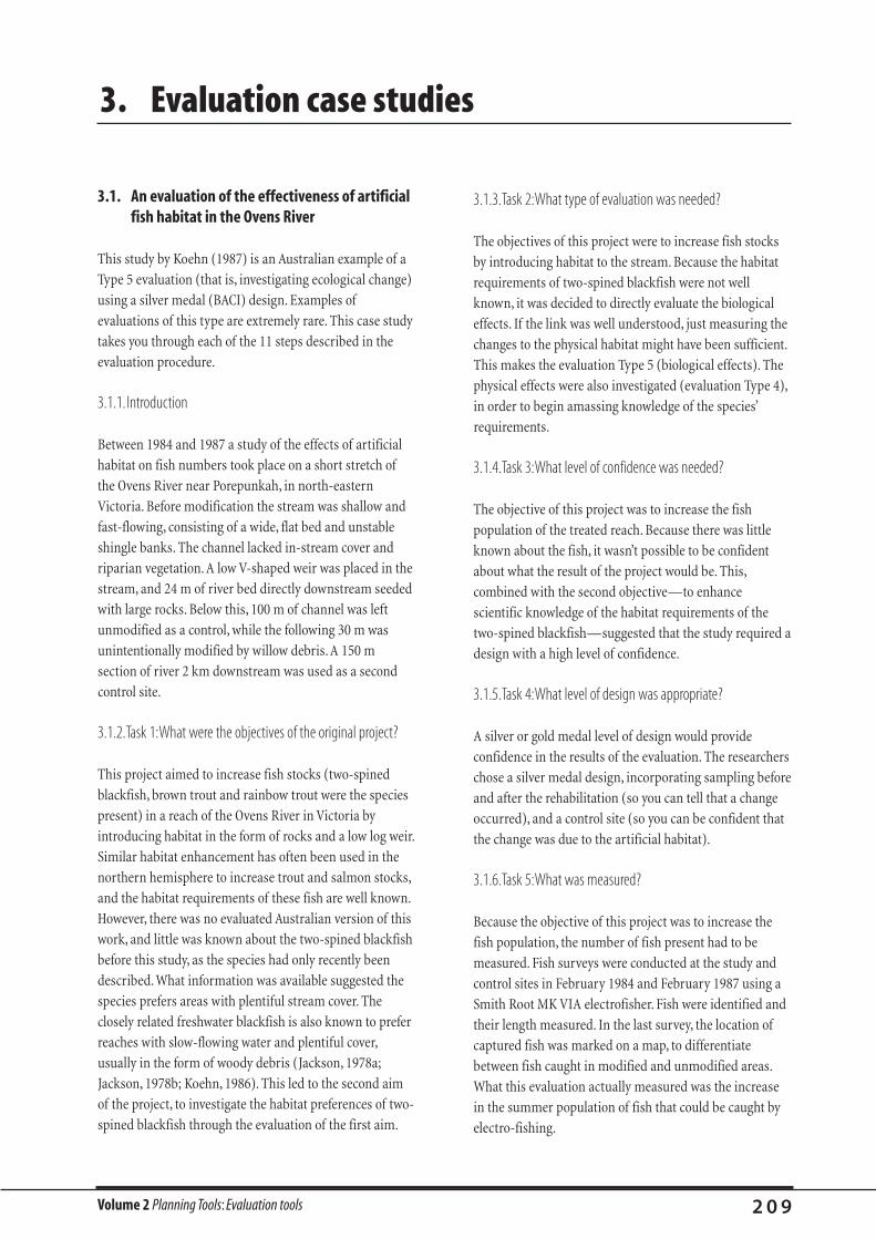
Volume 2 Planning Tools: Evaluation tools 2 0 9
3.1. An evaluation of the effectiveness of artificialfish habitat in the Ovens River
This study by Koehn (1987) is an Australian example of a
Type 5 evaluation (that is, investigating ecological change)
using a silver medal (BACI) design. Examples of
evaluations of this type are extremely rare. This case study
takes you through each of the 11 steps described in the
evaluation procedure.
3.1.1. Introduction
Between 1984 and 1987 a study of the effects of artificial
habitat on fish numbers took place on a short stretch of
the Ovens River near Porepunkah, in north-eastern
Victoria. Before modification the stream was shallow and
fast-flowing, consisting of a wide, flat bed and unstable
shingle banks. The channel lacked in-stream cover and
riparian vegetation. A low V-shaped weir was placed in the
stream, and 24 m of river bed directly downstream seeded
with large rocks. Below this, 100 m of channel was left
unmodified as a control, while the following 30 m was
unintentionally modified by willow debris. A 150 m
section of river 2 km downstream was used as a second
control site.
3.1.2.Task 1:What were the objectives of the original project?
This project aimed to increase fish stocks (two-spined
blackfish, brown trout and rainbow trout were the species
present) in a reach of the Ovens River in Victoria by
introducing habitat in the form of rocks and a low log weir.
Similar habitat enhancement has often been used in the
northern hemisphere to increase trout and salmon stocks,
and the habitat requirements of these fish are well known.
However, there was no evaluated Australian version of this
work, and little was known about the two-spined blackfish
before this study, as the species had only recently been
described. What information was available suggested the
species prefers areas with plentiful stream cover. The
closely related freshwater blackfish is also known to prefer
reaches with slow-flowing water and plentiful cover,
usually in the form of woody debris (Jackson, 1978a;
Jackson, 1978b; Koehn, 1986). This led to the second aim
of the project, to investigate the habitat preferences of two-
spined blackfish through the evaluation of the first aim.
3.1.3.Task 2:What type of evaluation was needed?
The objectives of this project were to increase fish stocks
by introducing habitat to the stream. Because the habitat
requirements of two-spined blackfish were not well
known, it was decided to directly evaluate the biological
effects. If the link was well understood, just measuring the
changes to the physical habitat might have been sufficient.
This makes the evaluation Type 5 (biological effects). The
physical effects were also investigated (evaluation Type 4),
in order to begin amassing knowledge of the species’
requirements.
3.1.4.Task 3:What level of confidence was needed?
The objective of this project was to increase the fish
population of the treated reach. Because there was little
known about the fish, it wasn’t possible to be confident
about what the result of the project would be. This,
combined with the second objective—to enhance
scientific knowledge of the habitat requirements of the
two-spined blackfish—suggested that the study required a
design with a high level of confidence.
3.1.5.Task 4:What level of design was appropriate?
A silver or gold medal level of design would provide
confidence in the results of the evaluation. The researchers
chose a silver medal design, incorporating sampling before
and after the rehabilitation (so you can tell that a change
occurred), and a control site (so you can be confident that
the change was due to the artificial habitat).
3.1.6.Task 5:What was measured?
Because the objective of this project was to increase the
fish population, the number of fish present had to be
measured. Fish surveys were conducted at the study and
control sites in February 1984 and February 1987 using a
Smith Root MK VIA electrofisher. Fish were identified and
their length measured. In the last survey, the location of
captured fish was marked on a map, to differentiate
between fish caught in modified and unmodified areas.
What this evaluation actually measured was the increase
in the summer population of fish that could be caught by
electro-fishing.
3. Evaluation case studies
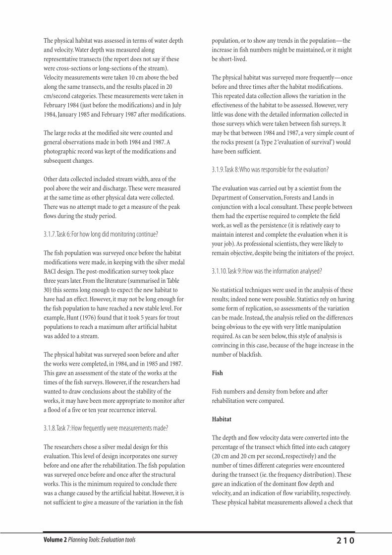
Volume 2 Planning Tools: Evaluation tools 2 1 0
The physical habitat was assessed in terms of water depth
and velocity. Water depth was measured along
representative transects (the report does not say if these
were cross-sections or long-sections of the stream).
Velocity measurements were taken 10 cm above the bed
along the same transects, and the results placed in 20
cm/second categories. These measurements were taken in
February 1984 (just before the modifications) and in July
1984, January 1985 and February 1987 after modifications.
The large rocks at the modified site were counted and
general observations made in both 1984 and 1987. A
photographic record was kept of the modifications and
subsequent changes.
Other data collected included stream width, area of the
pool above the weir and discharge. These were measured
at the same time as other physical data were collected.
There was no attempt made to get a measure of the peak
flows during the study period.
3.1.7.Task 6:For how long did monitoring continue?
The fish population was surveyed once before the habitat
modifications were made, in keeping with the silver medal
BACI design. The post-modification survey took place
three years later. From the literature (summarised in Table
30) this seems long enough to expect the new habitat to
have had an effect. However, it may not be long enough for
the fish population to have reached a new stable level. For
example, Hunt (1976) found that it took 5 years for trout
populations to reach a maximum after artificial habitat
was added to a stream.
The physical habitat was surveyed soon before and after
the works were completed, in 1984, and in 1985 and 1987.
This gave an assessment of the state of the works at the
times of the fish surveys. However, if the researchers had
wanted to draw conclusions about the stability of the
works, it may have been more appropriate to monitor after
a flood of a five or ten year recurrence interval.
3.1.8.Task 7:How frequently were measurements made?
The researchers chose a silver medal design for this
evaluation. This level of design incorporates one survey
before and one after the rehabilitation. The fish population
was surveyed once before and once after the structural
works. This is the minimum required to conclude there
was a change caused by the artificial habitat. However, it is
not sufficient to give a measure of the variation in the fish
population, or to show any trends in the population—the
increase in fish numbers might be maintained, or it might
be short-lived.
The physical habitat was surveyed more frequently—once
before and three times after the habitat modifications.
This repeated data collection allows the variation in the
effectiveness of the habitat to be assessed. However, very
little was done with the detailed information collected in
those surveys which were taken between fish surveys. It
may be that between 1984 and 1987, a very simple count of
the rocks present (a Type 2 ‘evaluation of survival’) would
have been sufficient.
3.1.9.Task 8:Who was responsible for the evaluation?
The evaluation was carried out by a scientist from the
Department of Conservation, Forests and Lands in
conjunction with a local consultant. These people between
them had the expertise required to complete the field
work, as well as the persistence (it is relatively easy to
maintain interest and complete the evaluation when it is
your job). As professional scientists, they were likely to
remain objective, despite being the initiators of the project.
3.1.10.Task 9:How was the information analysed?
No statistical techniques were used in the analysis of these
results; indeed none were possible. Statistics rely on having
some form of replication, so assessments of the variation
can be made. Instead, the analysis relied on the differences
being obvious to the eye with very little manipulation
required. As can be seen below, this style of analysis is
convincing in this case, because of the huge increase in the
number of blackfish.
Fish
Fish numbers and density from before and after
rehabilitation were compared.
Habitat
The depth and flow velocity data were converted into the
percentage of the transect which fitted into each category
(20 cm and 20 cm per second, respectively) and the
number of times different categories were encountered
during the transect (ie. the frequency distribution). These
gave an indication of the dominant flow depth and
velocity, and an indication of flow variability, respectively.
These physical habitat measurements allowed a check that

Volume 2 Planning Tools: Evaluation tools 2 1 1
the rehabilitation had actually changed conditions in the
stream, as well as helping in the interpretation of the
biological data.
The number of rocks present just after the habitat was
modified was compared with the number present at the
end of the evaluation.
3.1.11.Task 10:How much did this evaluation cost?
There was no indication of cost in the report. However, it is
likely the evaluation cost at least as much as the physical
works.
3.1.12.Task 11:What recording techniques were used?
During electro-fishing, the positions in the reach where
fish were caught were marked on a map. No other
information is available on recording techniques.
3.1.13.Results and conclusions
Fish
Two-spined blackfish were the main species caught in the
study. Some trout were caught, but their numbers were so
low that they are disregarded in this summary. Table 32
shows the overwhelming result that there were nine times
as many fish in the artificial rock habitat as expected, and
five times as many in the willow debris habitat, while fish
numbers in the unmodified stream did not increase.
Similar results are found when the results are expressed as
numbers of fish per 100 m2 of habitat. From this it seems
clear that the artificial habitat had a dramatic effect on fish
numbers. With only one survey before and one after
treatment, no statistical analyses of these results are
possible. In this study it may not matter because the
increase in fish numbers was so great. However, a more
subtle response to the rehabilitation might have required
some statistical analysis for a clear interpretation.
Table 32.The increase in blackfish numbers after the construction of
artificial habitat in the Ovens River.
River section Increase Fish per 100 m2
Rock area x 9 9
Unmodified area (control) x 1 1.1
Willow debris x 5 6.7
Habitat
The velocity transects revealed a greater flow complexity
after modification (9 velocity categories encountered
before compared with between 13 and 19 after). They also
showed an increase in both the slowest and fastest moving
water in the rocky section. By comparison, flow complexity
in the unmodified section had not changed, though the
proportion of high velocity flow had increased.
The comparison of the number of rocks present just after
the modifications and at the end of the study revealed that
a large portion of rocks had been covered by sediment, and
were therefore no longer providing fish habitat.
Conclusion
The researchers concluded that in-stream cover was
important to "fish species, especially the two-spined
blackfish", and "that the use of artificial cover can
dramatically increase" fish stock. It is not stated, but we
assume that the variation in flow velocity produced by the
works contributed to the improved habitat. Importantly,
there were few fish found in the deep pool formed
upstream of the structure, suggesting that the cover and
hydraulic habitat associated with the rocks, weir, and
willows were more important than the pool depth.
However, because the weir was not isolated from the rocks,
it is not really possible to separate the effects of the two
components of the rehabilitation.
The original objectives of this project were to increase
the fish population of the modified reach, and to
increase knowledge of the habitat preferences of the
two-spined blackfish. These have plainly both been met.
There was a nine-fold increase in two-spined blackfish
numbers, and it is now known that the species, in this
situation at least, prefers reaches with plentiful in-
stream cover and diverse hydraulics, including areas of
slow-flowing water.
3.2. An evaluation of the use of vegetation andstructure to control stream bank erosioncaused by bed degradation
An example from the Mississippi River, USA of a gold
medal Type 4 (physical effects) evaluation (Shields et al.,
1995a).
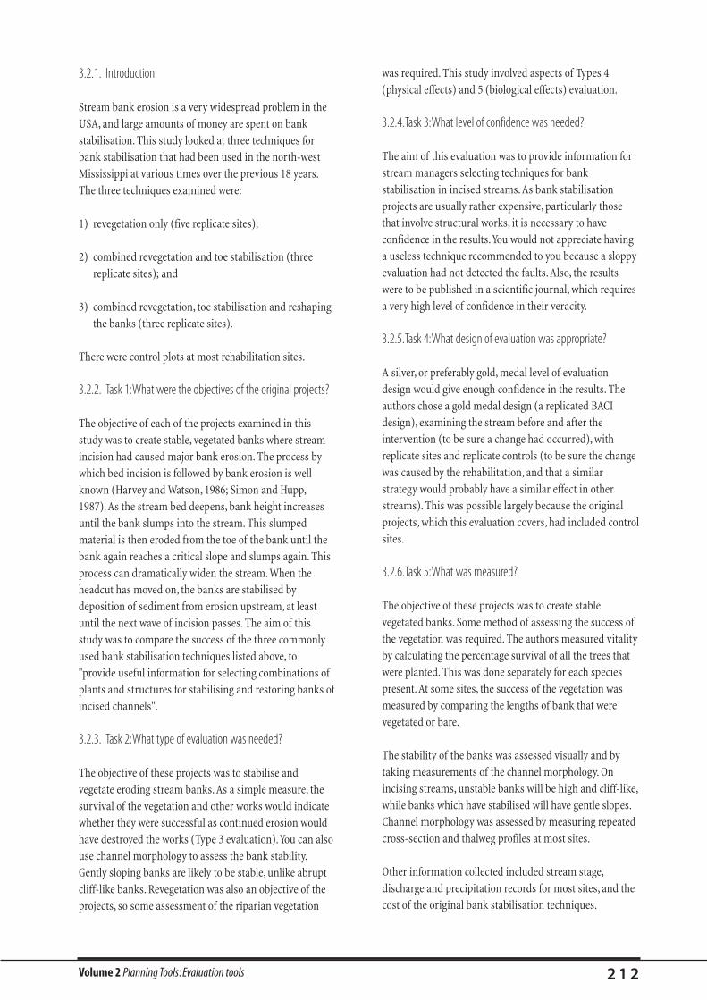
Volume 2 Planning Tools: Evaluation tools 2 1 2
3.2.1. Introduction
Stream bank erosion is a very widespread problem in the
USA, and large amounts of money are spent on bank
stabilisation. This study looked at three techniques for
bank stabilisation that had been used in the north-west
Mississippi at various times over the previous 18 years.
The three techniques examined were:
1) revegetation only (five replicate sites);
2) combined revegetation and toe stabilisation (three
replicate sites); and
3) combined revegetation, toe stabilisation and reshaping
the banks (three replicate sites).
There were control plots at most rehabilitation sites.
3.2.2. Task 1:What were the objectives of the original projects?
The objective of each of the projects examined in this
study was to create stable, vegetated banks where stream
incision had caused major bank erosion. The process by
which bed incision is followed by bank erosion is well
known (Harvey and Watson, 1986; Simon and Hupp,
1987). As the stream bed deepens, bank height increases
until the bank slumps into the stream. This slumped
material is then eroded from the toe of the bank until the
bank again reaches a critical slope and slumps again. This
process can dramatically widen the stream. When the
headcut has moved on, the banks are stabilised by
deposition of sediment from erosion upstream, at least
until the next wave of incision passes. The aim of this
study was to compare the success of the three commonly
used bank stabilisation techniques listed above, to
"provide useful information for selecting combinations of
plants and structures for stabilising and restoring banks of
incised channels".
3.2.3. Task 2:What type of evaluation was needed?
The objective of these projects was to stabilise and
vegetate eroding stream banks. As a simple measure, the
survival of the vegetation and other works would indicate
whether they were successful as continued erosion would
have destroyed the works (Type 3 evaluation).You can also
use channel morphology to assess the bank stability.
Gently sloping banks are likely to be stable, unlike abrupt
cliff-like banks. Revegetation was also an objective of the
projects, so some assessment of the riparian vegetation
was required. This study involved aspects of Types 4
(physical effects) and 5 (biological effects) evaluation.
3.2.4.Task 3:What level of confidence was needed?
The aim of this evaluation was to provide information for
stream managers selecting techniques for bank
stabilisation in incised streams. As bank stabilisation
projects are usually rather expensive, particularly those
that involve structural works, it is necessary to have
confidence in the results.You would not appreciate having
a useless technique recommended to you because a sloppy
evaluation had not detected the faults. Also, the results
were to be published in a scientific journal, which requires
a very high level of confidence in their veracity.
3.2.5.Task 4:What design of evaluation was appropriate?
A silver, or preferably gold, medal level of evaluation
design would give enough confidence in the results. The
authors chose a gold medal design (a replicated BACI
design), examining the stream before and after the
intervention (to be sure a change had occurred), with
replicate sites and replicate controls (to be sure the change
was caused by the rehabilitation, and that a similar
strategy would probably have a similar effect in other
streams). This was possible largely because the original
projects, which this evaluation covers, had included control
sites.
3.2.6.Task 5:What was measured?
The objective of these projects was to create stable
vegetated banks. Some method of assessing the success of
the vegetation was required. The authors measured vitality
by calculating the percentage survival of all the trees that
were planted. This was done separately for each species
present. At some sites, the success of the vegetation was
measured by comparing the lengths of bank that were
vegetated or bare.
The stability of the banks was assessed visually and by
taking measurements of the channel morphology. On
incising streams, unstable banks will be high and cliff-like,
while banks which have stabilised will have gentle slopes.
Channel morphology was assessed by measuring repeated
cross-section and thalweg profiles at most sites.
Other information collected included stream stage,
discharge and precipitation records for most sites, and the
cost of the original bank stabilisation techniques.

Volume 2 Planning Tools: Evaluation tools 2 1 3
3.2.7.Task 6:For how long did monitoring continue?
This was an opportunistic evaluation, incorporating
suitable experimental plots of varying ages. As a result, the
monitoring periods at different sites varied from only a
single growing season to 18 years. A single growing season
is really not long enough to assess the success of the
stabilisation. The authors point out that, at some of the
older sites, high early mortality in the planted vegetation
was followed by successful bank stabilisation with natural
regeneration of native species occurring within three
years. As the longer periods of monitoring were sufficient
to show this natural revegetation, this suggests that
monitoring for slightly over three years would be sufficient
to assess the success of the vegetation.
The success of bank stabilisation works also depends on
whether they have been tested by high flows. This varied
between sites, with some experiencing moderate floods,
whilst two others had record floods. However, the
construction of bank protection seems to have occurred
in periods of below average flow at many sites. For those
sites that have not yet experienced floods, it may be
premature to conclude the works have stabilised the
banks.
3.2.8.Task 7:How frequent were measurements made?
Because this evaluation was an overview of many
individual projects, the frequency of monitoring varied
from site to site. It is not clear from the published paper
how frequently monitoring occurred. To assess the long-
term stability of the stream banks, it might be possible to
take measurements only once before and once after the
modifications were complete. This would tell you if the
project was successful. However, in those cases where the
works failed, such a monitoring regime would miss any
chance of telling you what caused the failure. Ideally,
monitoring should occur more frequently than this, for
example, once a year until the vegetation was established,
or after every flood above a certain size.
3.2.9.Task 8:Who was responsible for the evaluation?
The evaluation was carried out by the authors (two
hydraulic engineers and one ecologist) who were employed
by the US Department of Agriculture. Between them they
had the expertise to complete the monitoring, as well as
the persistence. As professional scientists, they likely had
the ability to remain objective.
3.2.10.Task 9:How was the information analysed?
This evaluation included many individual projects of
different ages. As a result, information was not available in
the same form for each site, and the length of monitoring
period varied. This would have made statistical analysis
very difficult. Instead, the results were examined in an
‘eyeballing’ style of analysis; in this case basically a
qualitative comparison of descriptions of sites with each of
the three rehabilitation strategies.
3.2.11.Task 10:How much did this evaluation cost?
The cost of the evaluation is not given in the published
paper.
3.2.12.Task 11:What recording techniques were used?
Techniques for recording information in the field are not
reported in the published paper.
3.2.13.Results and conclusions
The results showed that vegetation by itself was not
sufficient to stabilise stream banks while the process of
bed erosion went unchecked. However, if the bed was no
longer eroding, natural recolonisation of unplanted control
plots was generally as successful as manual revegetation
(the proximity of a seed source is not commented on).
Where toe protection was combined with revegetation,
banks still failed but as the toe protection prevented scour
from eroding the spoil, a stable angle of bank was formed
and recolonised by local trees. This occurred even where
the stream bed eroded slightly. Where banks were shaped
along with the other treatments they "remained well
vegetated and stable" at all sites.
3.3. Evaluating structural works on the HunterRiver, New South Wales
This study by Nagel (1995) is an example of a Type 4
(physical effects) evaluation, using a Tin medal design.
3.3.1. Introduction
Large floods in the 1950s triggered catastrophic widening of
streams in the Hunter River catchment (New South Wales).
To stabilise the streams, many millions of dollars worth of
structures (mesh embayments) were built to artificially

Volume 2 Planning Tools: Evaluation tools 2 1 4
narrow the stream along a stable alignment, incorporating
willow plantations. New alignments and widths were
determined by comparison with nearby stable sections of
stream. The performance of 28 bank protection structures
along 3.4 km of Baerami Creek (a tributary of the Hunter
River) was evaluated in 1994 by Fiona Nagel (Nagel, 1995),
then an honours student at Macquarie University, now
Resource Officer, Riverine Management, Department of
Land and Water Conservation North Coast Region, NSW.
3.3.2.Task 1:What were the objectives of the original project?
The original goals of the work were to "protect assets from
abrupt channel changes during floods, and provide a
stable unobstructed channel for the efficient conveyance of
water and sediment". These objectives are not couched in
terms that can be measured easily. It would have been
better if they had included some indication of which assets
should be protected, what size floods the channel should
convey without significant erosion, and what the stable,
unobstructed channel should look like in terms of, say,
width, depth and roughness.
3.3.3.Task 2:What type of evaluation was needed?
The first objective of this project was to prevent abrupt
channel changes during floods. This required a Type 4
(physical effects) evaluation to measure the channel
morphology before and after major floods to quantify any
erosion. The second objective was to provide a stable
channel for the efficient conveyance of water and
sediment. As this involved creating a new channel in the
old over-widened bed, this objective could be measured in
a Type 2 evaluation (survival), to see if the constructed
channel is still present, or Type 4 (physical effects) to see if
the new channel is capable of conveying water and
sediment. The evaluation by Nagel (1995) was a
combination of types 2 and 4.
3.3.4.Task 3:What level of confidence was needed?
The evaluation was aimed at assessing, for the benefit of
stream managers, the value of stream stabilisation works,
so that current stream stabilisation practices can be
improved. A moderate level of confidence was sufficient.
3.3.5.Task 4:What design of evaluation was appropriate?
A bronze or silver medal design was appropriate for a
moderate level of confidence. However, this evaluation was
handicapped by being designed 27 years after the
completion of the structural works, rather than during the
project planning. There was little precise information
available on the pre-works channel. No control sites were
included in the original project; they would have allowed a
comparison of the natural recovery of the river with the
effects of the structural works. Instead, the evaluation was
limited to comparing the original design of structures
with their condition in 1995, and studying the river’s
geomorphic condition. However, 28 replicate site were
incorporated. This would be classified as a tin medal
design with replication.
3.3.6.Task 5:What was measured?
Collecting measurements for an evaluation designed after a
project is completed is usually difficult. Relevant information
is often not collected before work commences, and
evaluation must rely on inferring the original condition of
the stream from sources such as old surveys or air photos.
Evaluating the survival of structural works usually
involves comparing the present condition of a structure
with its ‘as-built’ condition. In this case, this involved
detailed examination of historical records including old
surveys and field ganger reports detailing the
construction. Where these were missing, construction
dates for the works had to be inferred by willow tree core
dating or extrapolation from old photos. The channel
morphology was measured to detect changes in channel
alignment, sinuosity and width, and bed level changes.
Interpretation of aerial photographs yielded information
on channel changes. Additional information of stream
gauge and rainfall records was obtained where possible,
but these records were incomplete.
3.3.7.Task 6:For how long did monitoring continue?
The measurements of the channel and channel training
structures took place between 1 and 27 years after
construction, depending on the age of the works. Twenty-
seven years seems a very long monitoring period, but
nevertheless it did not include any floods of the magnitude
which caused the original channel widening. As the project
objectives didn’t specify what size floods the structures
should withstand, it is unclear if this monitoring period is
sufficient.
3.3.8.Task 7:How frequently were measurements made?
The structures were examined once in the 27 years since
construction. This is sufficient to measure gross changes

Volume 2 Planning Tools: Evaluation tools 2 1 5
since construction, but not to provide information on the
trends in channel development, or suggest what events
may have caused failure, where it occurred. Monitoring
after every flood of a given size is ideal.
3.3.9.Task 8:Who was responsible for the evaluation?
No evaluation appears to have been built into the original
project design. Fiona Nagel, an honours student from the
School of Earth Sciences at Macquarie University was
responsible for the post hoc evaluation. Such a person
would have access to the expertise required to complete
the monitoring.
3.3.10.Task 9:How was the information analysed?
Changes in the channel alignment at each field site were
put into discrete categories, including upstream or
downstream meander translation, bend rotation or
extension, or movement of the channel away from the
works. The channel-training structures were ranked in
terms of effectiveness. An example of a ‘least effective’ site
may have erosion into the bank the structure was designed
to protect, as well as upstream and downstream erosion,
and few surviving planted trees.
3.3.11.Task 10:How much did this evaluation cost?
This evaluation was part of a student project, and costs
were therefore low, around $3,000. However, this included
unpaid labour of almost 6 weeks in the field, and much of
two years’ part-time study.
3.3.12.Task 11:What recording technique was used?
Data were recorded in the field, on pre-printed forms.
3.3.13.Results and conclusions
The stabilisation works examined here were not really
designed with evaluation in mind. It is possible to evaluate
the outputs of the project—the stabilisation structures
and vegetation. These generally seem to have survived,
although the willows used at the older sites are now
reaching the end of their lives. However, it is harder to say
anything concrete about the outcomes of the project. The
structures have controlled erosion of the bends that they
were designed to protect. However, the stream has
narrowed and developed a new meander wavelength.
Because of this, the banks are now eroding up and
downstream of the works. Nagel (1995) suggested that
such adjustments were an inevitable result of the flow
regime. Because there was no control site, it is difficult to
say if the current situation is preferable to one where no
stabilising work was done. Given the lower flow regime
since the installation of the structures, it is possible that
the observed contraction of the channel would have
occurred without any intervention. This lack of high flows
also means the structures have never been tested by floods
as large as those of the 1950s. Thus, it is difficult to decide
whether or not to call the works a success, or just a case of
serendipity.

• Why stakeholders may not support your plan
• Setting priorities for stream rehabilitation
• Legislative and administrative constraints
• Benefit–cost analysis of stream rehabiliationprojects
• The geographic information system (GIS) as astream rehabilitation tool
• Some costs of stream rehabilitation activities
• Bibliography of some technical informationavailable in Australia
MISCELLANEOUSPLANNING TOOLS

1.2. They can see that there is a problem, but it’snot their problem
Stream rehabilitation benefits the community and future
generations as well as landholders. In this situation,
landholders may feel that the responsibility for
rehabilitation (and its costs) lies with the community
rather than with them.
1.3. Stakeholders disagree with the streammanager about the cause of the problem
Often, people will agree with the stream manager that
there is a problem, but vehemently disagree about its
cause. Years of observation of stream behaviour,
including short and long-term changes, often means that
people have formed ideas about the causes of stream
problems. However, they may not have an understanding
of the geomorphic or biological processes underlying
changes to the stream. People may mistake association
with causation, as in the following example. This is not
to say that stakeholders can’t be right and stream
managers wrong, rather, just because somebody has
observed something for a long time does not
automatically mean that they understand the cause, or
know the best solution.
Volume 2 Planning Tools: Miscellaneous planning tools 2 1 7
WHY STAKEHOLDERS MAY NOT SUPPORTYOUR PLAN
Compiled with the assistance of Neville Oddie*
The support of other people is critical for the long-term
success of all stream rehabilitation projects. This will mean
not only getting support from landowners, but also from
any other stakeholders in the stream, including anyone
with an interest in the general community, government
departments, and industry. In Step 2: Who shares your goals
for the stream? in the Stream rehabilitation procedure,
Volume 1, we discussed how to go about getting people’s
support. In this section, we expand on this, describing
seven reasons why other stakeholders in the stream might
not support a rehabilitation plan, and how you might go
about finding a compromise that everyone can agree on.
The following applies particularly to rural landholders.
1.1. Landholders do not recognise that there is a problem
In many situations, landholders will have a different vision
of their stream than do stream managers. Farmers may
see streams in terms of the drainage and water supply
functions, or as a nuisance (a source of pests or weeds, or
floods). Alternatively, landowners may have a vision of the
stream based on, for example, aesthetics, flood
conveyance, stability or trout fishing, rather than the
broader environmental goals of the stream manager.
Landholders may well see no problem with a stream that
has very little ecological value in its present state.
Possible solutionsChange the landholder’s vision of the stream.
Set up demonstration sites that show what can be achieved.
Involve the landholders in the problem identification process.
Possible solutionsKnow the cost and any other consequences of the project from
the outset (see Natural channel design, this Volume, for
methods of estimating flooding and erosion consequences of
the works). Knowing the cost of the project makes it easier to
negotiate compromises.
Know the value of benefits to the farm that may result from
the project (see, for example, the end of this chapter).
*Earth Resources Analysis, RMB 435, Snake Valley,Victoria 3351. Ph and Fax: (03) 5344 9471 Email: [email protected]
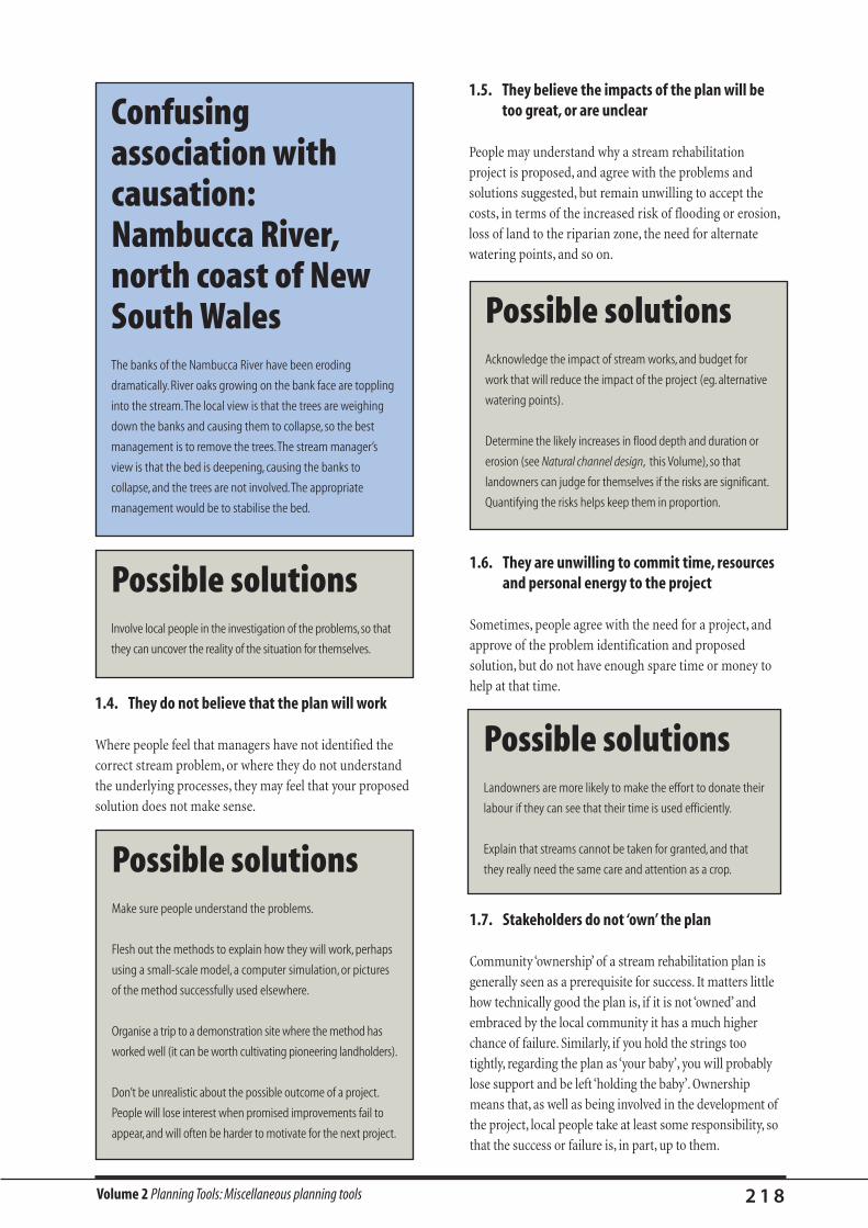
2 1 8
1.4. They do not believe that the plan will work
Where people feel that managers have not identified the
correct stream problem, or where they do not understand
the underlying processes, they may feel that your proposed
solution does not make sense.
1.5. They believe the impacts of the plan will betoo great, or are unclear
People may understand why a stream rehabilitation
project is proposed, and agree with the problems and
solutions suggested, but remain unwilling to accept the
costs, in terms of the increased risk of flooding or erosion,
loss of land to the riparian zone, the need for alternate
watering points, and so on.
Confusingassociation withcausation:Nambucca River,north coast of NewSouth WalesThe banks of the Nambucca River have been eroding
dramatically. River oaks growing on the bank face are toppling
into the stream.The local view is that the trees are weighing
down the banks and causing them to collapse, so the best
management is to remove the trees.The stream manager’s
view is that the bed is deepening, causing the banks to
collapse, and the trees are not involved.The appropriate
management would be to stabilise the bed.
Possible solutionsInvolve local people in the investigation of the problems,so that
they can uncover the reality of the situation for themselves.
Possible solutionsMake sure people understand the problems.
Flesh out the methods to explain how they will work, perhaps
using a small-scale model, a computer simulation, or pictures
of the method successfully used elsewhere.
Organise a trip to a demonstration site where the method has
worked well (it can be worth cultivating pioneering landholders).
Don’t be unrealistic about the possible outcome of a project.
People will lose interest when promised improvements fail to
appear, and will often be harder to motivate for the next project.
Possible solutionsAcknowledge the impact of stream works, and budget for
work that will reduce the impact of the project (eg. alternative
watering points).
Determine the likely increases in flood depth and duration or
erosion (see Natural channel design, this Volume), so that
landowners can judge for themselves if the risks are significant.
Quantifying the risks helps keep them in proportion.
1.6. They are unwilling to commit time, resourcesand personal energy to the project
Sometimes, people agree with the need for a project, and
approve of the problem identification and proposed
solution, but do not have enough spare time or money to
help at that time.
Possible solutionsLandowners are more likely to make the effort to donate their
labour if they can see that their time is used efficiently.
Explain that streams cannot be taken for granted, and that
they really need the same care and attention as a crop.
1.7. Stakeholders do not ‘own’ the plan
Community ‘ownership’ of a stream rehabilitation plan is
generally seen as a prerequisite for success. It matters little
how technically good the plan is, if it is not ‘owned’ and
embraced by the local community it has a much higher
chance of failure. Similarly, if you hold the strings too
tightly, regarding the plan as ‘your baby’, you will probably
lose support and be left ‘holding the baby’. Ownership
means that, as well as being involved in the development of
the project, local people take at least some responsibility, so
that the success or failure is, in part, up to them.
Volume 2 Planning Tools: Miscellaneous planning tools
Volume 2 Planning Tools: Miscellaneous planning tools 2 1 9
1.8. Some economic benefits of vegetation on farms
Provided by Mike Askey-Doran*
NOTE: Most of these figures come from studies of patches of
remnant bush on properties, not specifically from riparian
zones.
Vegetation acts as a windbreak, sheltering stock from
extremes of cold, wind and rain, and reducing death rates
in new-born lambs or newly shorn sheep. In a trial in
south-western Victoria, a 5-day period of cold, wet and
windy weather led to the deaths of 40% of lambs in
exposed areas compared with 12% in sheltered areas (Reid
and Bird, 1990). On one bitterly cold night in 1987, up to
30,000 sheep died in western Victoria, while 1,600 sheep
(worth $80,000) that were moved into remnant bush
survived.
Trees provide shade, which reduces heat stress. Heat stress
has been shown to reduce the fertility of both cattle and
sheep (Bird et al., 1984). Pregnant cows are more prone to
abort when heat stressed, and new-born calves are more
likely to be undersized (Reid and Bird, 1990). Heat stress
affects appetite which leads to reductions in weight gain
and wool production. Research has demonstrated that cows
and calves grazing with adequate shade have weight gains
up to 0.6 kg daily compared with 0.3 kg for stock without
shade.Work in Armidale has demonstrated that shelter
leads to both increased wool production (up to 31%) and
higher live-weights (up to 6 kg). Shade is especially
important for dairy cattle, as milk production drops off as
temperatures rise above 20°C (Reid and Bird, 1990).
Fencing riparian land can prevent the loss of valuable
stock, such as dairy cattle, which may drown if they fall
into a stream.
Riparian vegetation acts as a windbreak, reducing wind
velocities and consequently reducing water losses from
both soil and crops. Pasture and crop yields can be as
much as 20–30% higher on the downwind side of a
shelterbelt compared with unprotected crops. The
windbreak can be effective for a distance up to ten times
the height of the windbreak (Sturrock, 1981).
Anecdotal evidence suggests that retaining remnant
vegetation can add up to 10% to the sale price of rural
properties. Agricultural and cattle properties in Western
Australia that have retained remnant vegetation have been
favoured over over-developed properties. People
purchasing land are valuing remnant bushland as a real
asset and are adding this value into their purchase price
(O’Brien, 1996).
Possible solutionsPeople should be involved in the entire process of planning
and rehabilitating the stream.
People should be given some power over the project.This may
be possible by defining basic boundaries the plan must stay
within (eg. it must lead to a long-term increase in biodiversity),
but within those bounds the community plays a major role in
deciding what form the project will take.
*Parks and Wildlife Service, GPO Box 44A, Hobart,Tasmania 7001. Ph: (03) 6233 6168.
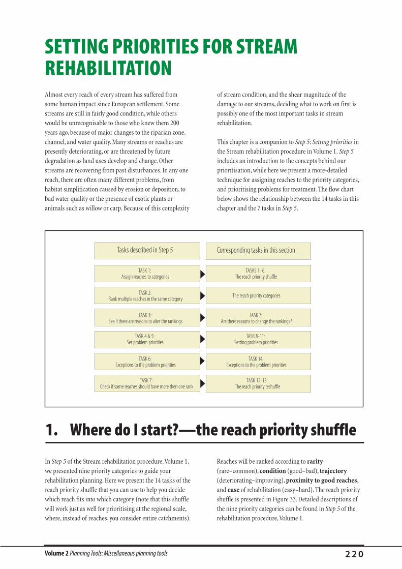
of stream condition, and the shear magnitude of the
damage to our streams, deciding what to work on first is
possibly one of the most important tasks in stream
rehabilitation.
This chapter is a companion to Step 5: Setting priorities in
the Stream rehabilitation procedure in Volume 1. Step 5
includes an introduction to the concepts behind our
prioritisation, while here we present a more-detailed
technique for assigning reaches to the priority categories,
and prioritising problems for treatment. The flow chart
below shows the relationship between the 14 tasks in this
chapter and the 7 tasks in Step 5.
Volume 2 Planning Tools: Miscellaneous planning tools 2 2 0
Almost every reach of every stream has suffered from
some human impact since European settlement. Some
streams are still in fairly good condition, while others
would be unrecognisable to those who knew them 200
years ago, because of major changes to the riparian zone,
channel, and water quality. Many streams or reaches are
presently deteriorating, or are threatened by future
degradation as land uses develop and change. Other
streams are recovering from past disturbances. In any one
reach, there are often many different problems, from
habitat simplification caused by erosion or deposition, to
bad water quality or the presence of exotic plants or
animals such as willow or carp. Because of this complexity
SETTING PRIORITIES FOR STREAMREHABILITATION
TASK 1: Assign reaches to categories
TASK 2: Rank multiple reaches in the same category
TASK 3: See if there are reasons to alter the rankings
TASK 4 & 5: Set problem priorities
TASK 6: Exceptions to the problem priorities
TASK 7: Check if some reaches should have more then one rank
TASKS 1- 6: The reach priority shuffle
The reach priority categories
TASK 7: Are there reasons to change the rankings?
TASK 8-11: Setting problem priorities
TASK 14: Exceptions to the problem priorities
TASK 12-13: The reach priority reshuffle
Tasks described in Step 5 Corresponding tasks in this section
In Step 5 of the Stream rehabilitation procedure,Volume 1,
we presented nine priority categories to guide your
rehabilitation planning. Here we present the 14 tasks of the
reach priority shuffle that you can use to help you decide
which reach fits into which category (note that this shuffle
will work just as well for prioritising at the regional scale,
where, instead of reaches, you consider entire catchments).
Reaches will be ranked according to rarity
(rare–common), condition (good–bad), trajectory
(deteriorating–improving), proximity to good reaches,
and ease of rehabilitation (easy–hard). The reach priority
shuffle is presented in Figure 33. Detailed descriptions of
the nine priority categories can be found in Step 5 of the
rehabilitation procedure,Volume 1.
1. Where do I start?—the reach priority shuffle
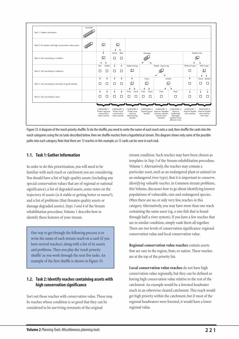
Volume 2 Planning Tools: Miscellaneous planning tools 2 2 1
1.1. Task 1: Gather information
In order to do this prioritisation, you will need to be
familiar with each reach or catchment you are considering.
You should have a list of high-quality assets (including any
special conservation values that are of regional or national
significance), a list of degraded assets, some notes on the
trajectory of assets (is it stable or getting better or worse?),
and a list of problems (that threaten quality assets or
damage degraded assets). Steps 3 and 4 of the Stream
rehabilitation procedure,Volume 1 describe how to
identify these features of your stream.
1.2. Task 2: Identify reaches containing assets withhigh conservation significance
Sort out those reaches with conservation value. These may
be reaches whose condition is so good that they can be
considered to be surviving remnants of the original
stream condition. Such reaches may have been chosen as
templates in Step 3 of the Stream rehabilitation procedure,
Volume 1. Alternatively, the reaches may contain a
particular asset, such as an endangered plant or animal (or
an endangered river type), that it is important to conserve.
Identifying valuable reaches, in Common stream problems,
this Volume, discusses how to go about identifying known
populations of vulnerable, rare and endangered species.
Often there are no, or only very few, reaches in this
category. Alternatively, you may have more than one reach
containing the same asset (eg. a rare fish that is found
through half a river system). If you have a few reaches that
are in similar condition, simply rank them all together.
There are two levels of conservation significance: regional
conservation value and local conservation value.
Regional conservation value reaches contain assets
that are rare in the region, State, or nation. These reaches
are at the top of the priority list.
Local conservation value reaches do not have high
conservation value regionally, but they can be defined as
having high conservation value relative to the rest of the
catchment. An example would be a forested headwater
reach in an otherwise cleared catchment. This reach would
get high priority within the catchment, but if most of the
regional headwaters were forested, it would have a lower
regional value.
Figure 33. A diagram of the reach priority shuffle.To do the shuffle, you need to write the name of each reach onto a card, then shuffle the cards into the
reach categories using the six tasks described below. Here we shuffle reaches from a hypothetical stream.This diagram shows only some of the possible
paths into each category. Note that there are 13 reaches in this example, so 13 cards can be seen in each task.
Task 1: Gather information
Unsorted
Det. Deteriorating Without hope With hope
Close
Stable - Improving
CloseDistant Distant
Easy Hard Easy Hard Easy Hard
Average Basket case
Stable
BadGood
Task 2: ID reaches with high conservation value assets
Task 3: Sort according to condition
Task 4: Sort according to trajectory
Task 5: Sort according to proximity to good reaches
Task 6: Sort according to ease
CATEGORY 1Protect regional
conservation value reaches
CATEGORY 2Protect local conservation value reaches
CATEGORY 3Protect and
improve deteriorating
reaches
CATEGORY 4Expand good
reaches
CATEGORY 5Improve impeded recovery reaches
(easily fixed reaches)
CATEGORY 6Improve
moderately damaged
reaches (more difficult to fix)
CATEGORY 7Improve basket case reaches
CATEGORY 8Improve basket case reaches
with hope
One way to get through the following process is to
write the name of each stream reach on a card (if you
have several reaches), along with a list of its assets
and problems. Then you play the ‘reach priority
shuffle’ as you work through the next five tasks. An
example of the first shuffle is shown in Figure 33.
Volume 2 Planning Tools: Miscellaneous planning tools 2 2 2
1.3. Task 3: Sort the reaches according to condition
Preserving reaches in good condition should be a major
aim of stream rehabilitation, so the next task is to rank the
reaches according to their condition.All the reaches in very
good condition should already be in the regional and local
conservation categories. If you have more than one reach in
either of these groups, then you can use their relative
condition to decide which is a higher priority. The reaches
you have not yet assigned to a category you should split into
two groups: an average group, and a basket-case group.
The average group contains all the reaches in average
condition—not specially good or bad.You will probably
have many reaches in this group—they will be divided
into smaller categories in the following tasks. At this stage,
they are the second-lowest priority.
The basket-case reaches are in extremely bad condition.
They would require enormous effort to rehabilitate, with
small chances of success. These reaches will be your lowest
priority.
1.4. Task 4: Sort the reaches according to trajectory
How the condition of the reach will change over time can
be important when deciding on priorities. It is usually
more efficient to stabilise deteriorating reaches now, rather
than having to fix them later. So reaches that are
deteriorating are a higher priority than reaches that are
stable. Reaches that are presently improving by themselves
are the lowest priority. Thus, where you have more than
one reach in a category, rank them according to their
trajectory.You should break up the average group into a
deteriorating category, and a stable–improving group.
The basket-case group should be broken into basket case
without hope (the deteriorating and stable reaches, that
will not recover without help, such as the saline streams of
Western Australia), and basket case with hope
(improving reaches, that might eventually recover
naturally, such as the incised lowland streams of coastal
New South Wales).
1.5. Task 5: Sort the reaches according to theirproximity to a reach in good condition
It is easiest to improve the condition of the stream by
expanding an area in good condition, rather than trying to
create a new island of improved stream amongst the
degraded reaches. There are two reasons for this. First,
although quality assets can be isolated within an
otherwise degraded setting (a healthy riparian zone beside
a stream with a sand slug, for example), their value is
greatest when combined with other assets to form a
complete stream community. Secondly, the recovery of
plant and animal communities is generally fastest when
there is a healthy community close by. This is because
colonising individuals will find the new habitat faster if
there is no barrier of inhospitable degraded reach (see
Recovery of disturbed stream systems in Australia, in Stream
rehabilitation concepts,Volume 1, for a discussion of this).
In order of priority, you should work on:
• reaches with a mix of high-quality assets and some
degraded assets (eg. a reach with a good riparian zone,
and good in-stream habitat, but poor water quality);
• poor quality reaches that link two reaches in good
condition;
• poor quality reaches connected by one end to a reach in
good condition; and
• poor quality reaches that are distant from good quality
reaches.
Thus, if two or more reaches still have the same priority,
rank them according to how close they are to a reach in
good condition. Split the stable–improving group into a
category of reaches that are close to good reaches, and a
group of distant reaches.
1.6. Task 6: Sort the reaches according to how easythey are to rehabilitate
If you have a choice between two similar tasks, it is
sensible to do the easier task first. Thus, this final
ranking of reaches is done according to how easy it would
be to fix each reach. For example, you may have a reach
that has bad condition, and is stable because the natural
recovery is impeded. Its condition could be dramatically
improved by a small intervention. So, if any two reaches
still have the same priority, you can rank them according
to how easy they would be to rehabilitate. Split the
distant group into a category of easily fixed impeded
recovery reaches, and a category of more difficult
moderately damaged reaches.

Volume 2 Part 1: Identifying valuable reaches? 2 2 3
1.7. The reach priority categories
You have now finished the first stage of the reach priority
shuffle, and should have eight categories of priorities.
Where you have more than one reach in a category, you
should have separated them on the grounds of condition,
trajectory, proximity, and ease of rehabilitation. The full
shuffle is shown in Figure 1. The eight categories, with a
brief description, are listed below, and can be read about in
more detail in Step 5: Setting priorities, in the Stream
rehabilitation procedure,Volume 1. Note that there is one
extra category—reaches in good condition that are
protected from threats fit into Category 0. How a reach
arrives in this category is revealed in the next section.
Category Zero: Reaches in good condition throughout,that
are already protected. Reaches in this category need nothing
done to them.There are no active threats, and they have been
protected against any potential threats.All the assets in the
reach are in good condition.All this reach needs is a watchful
eye, to check for the development of new threats in the future.
Category One: Protecting regional conservation value
reaches. The highest priority is to preserve those reaches
that are important nationally or regionally. These could
contain endangered species or communities, or be a good
quality fragment of a once common stream type.
Category Two: Protecting local conservation value
reaches. These reaches are surviving remnants of the
original stream condition. They do not fit into Category 1,
because they are common in the region, but they are still
important assets.
Category Three: Protecting and improving deteriorating
reaches. Some reaches will already be damaged, but their
condition is continuing to deteriorate. It is usually more
efficient to stop further deterioration than to wait for the
damage to reach a plateau, and then try to fix it.
Category Four: Expand good reaches. Expand good
areas of the stream, by:
• improving reaches with some good-quality assets and
some degraded assets;
• improving poor-quality reaches that link two good
quality reaches; and
• improving poor-quality reaches that are linked at one
end to a good-quality reach.
Category Five: Improve impeded recovery reaches
(easily fixed reaches). These are the reaches that are in
poor condition but have stabilised (ie. their condition is
not deteriorating). A natural recovery process ought to be
occurring, but some stream problems prevent this. If you
identify and fix that problem, you can allow the natural
recovery to do the hard work of improving the stream
condition.
Category Six: Improve moderately damaged reaches
(more difficult to fix). These are reaches that are
damaged by human impact, but have good potential to
recover at reasonable cost. They differ from Category 5
reaches in that they require several interventions, rather
than just one.
Category Seven: Improve basket-case reaches. These are
reaches in very poor condition, and which have little
chance of recovering by themselves over time. Such
reaches will usually need very expensive and difficult
intervention if they are to recover.
Category Eight: Improve basket-case reaches with hope.
These are the reaches that are in very poor condition, but
which do have some chance of recovering themselves with
time. Such streams are also expensive and difficult to
artificially rehabilitate, but they have a pretty good chance
of recovering themselves over time.
1.8. Task 7: Are there reasons to change the reachpriority rankings (getting more bang for yourbuck)?
Having sorted your reaches into the categories, you may
decide to rearrange the order of priority in order to get the
most value for your rehabilitation dollar. This is discussed
in Step 5 of the Stream rehabilitation procedure in Volume
1. Briefly, you might decide to give a low priority reach
higher priority because:
• it will help muster community support;
• it will create a reach with regional conservation value;
• it is sometimes easier to start rehabilitation in the
small upstream reaches; or
• outputs from the reach will have a detrimental effect on
the lake, estuary or wetland that will ultimately receive
the water.

asset twice, once to protect it from future deterioration,
and again to improve its condition.
2.3. Task 10: Are there any fatal problems thatthreaten or damage the asset?
Fatal problems are so severe that they exclude assets from
the stream. They must be fixed first—there is no point
doing anything else in the stream until the fatal problem is
fixed. Extremely bad water quality, or a major barrier to
fish passage, are examples of fatal problems, as are sand
slugs, huge deposits of sand in the bed of the stream,
travelling slowly downstream. Sand slugs can fill a stream,
swamping all the in-stream habitat, and leaving very
shallow water flowing over a smooth sheet of mobile sand.
Not surprisingly, such a stream will support few aquatic
plants or animals. Until the sediment has moved through
the reach (this can take many decades) or has been
stabilised in some way, it will continue to swamp any
habitat, including any added to the stream artificially. Any
work on the stream must first tackle the sand slug to be
successful. Thus, fatal problems are the highest priority.
Volume 2 Planning Tools: Miscellaneous planning tools 2 2 4
Unfortunately, the task of prioritisation is not yet over.You
have now decided the order in which you will work on
your reaches. But in each reach, where do you start? If you
are lucky, there will be only a few problems that need
fixing, but it is more common for a single reach to have
lots of problems, all of different magnitude. How do you
work out where to start? Should you fix all the problems in
this reach before moving on to the next? The key is to
consider the importance of the assets that are threatened
by the different problems, and to remember that you
should protect all the valuable assets in all reaches before
you begin to improve the condition of the steam. Then the
problems are ranked by how fatal or limiting each
problem is for each asset. In order to work this out, it
might be necessary to ‘reshuffle’ the reaches. These tasks
are described below.
2.1. Task 8: Identify the most important assets inyour top-priority reach
In rehabilitation terms, a stream problem is only a
problem because it damages the natural assets of the
stream. For the top-priority reach, identify the most
important asset. Use the same principles as the reach
priority shuffle—rare before common, good condition
before bad, deteriorating before improving, close to other
assets before distant, and easy before hard. In a Category 1
reach, for example, the most important asset will be the
one with regional conservation value (eg. the rare species,
or pristine morphology).
2.2. Task 9: Identify the problems that threaten ordamage the asset
Which problems get priority depends whether you are in
the protection or improvement stage of your
rehabilitation. Does the asset that you are looking at need
protecting (ie. is it from a reach in Categories 1, 2 or 3)? In
this case, list all the problems that might cause the
condition of that asset to deteriorate. If you have already
protected any regional and local conservation assets, and
stabilised any deteriorating reaches, then you are ready to
improve the condition of the asset. In this case, you should
list all of the problems that prevent your asset from
improving. Note that this means you can look at the same
2. Which problem do I fix first?
A fatal problemDartmouth Dam releases cold water to the Mitta Mitta River
(Figure 34).The cold water has dramatically reduced the
number and diversity of native fish in the reach below the
dam (Koehn et al., 1997a). If your goal is to return native fish
populations to their original size and diversity, then there is
less point planting riparian vegetation (presently dominated
by willows), and improving in-stream habitat, when the water
will still be too cold for fish.You either fix the fatal problem of
water temperature, or you consider working elsewhere.
Note that although these problems might come from
within the reach, they could also come from
upstream (such as bad water quality, or sediment), or
from downstream (such as a feral animal population,
or an erosion head migrating upstream).You might
often find that protecting one reach means treating
problems elsewhere in the stream.
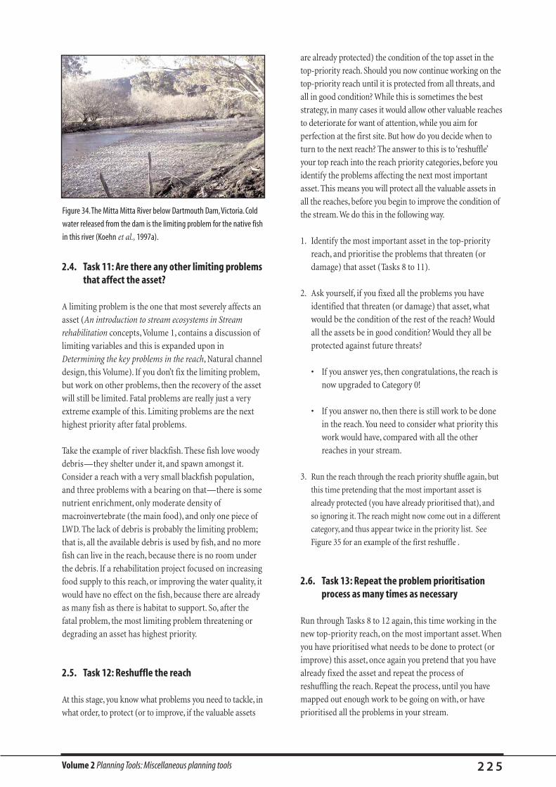
Volume 2 Planning Tools: Miscellaneous planning tools 2 2 5
2.4. Task 11: Are there any other limiting problemsthat affect the asset?
A limiting problem is the one that most severely affects an
asset (An introduction to stream ecosystems in Stream
rehabilitation concepts,Volume 1, contains a discussion of
limiting variables and this is expanded upon in
Determining the key problems in the reach, Natural channel
design, this Volume). If you don’t fix the limiting problem,
but work on other problems, then the recovery of the asset
will still be limited. Fatal problems are really just a very
extreme example of this. Limiting problems are the next
highest priority after fatal problems.
Take the example of river blackfish. These fish love woody
debris—they shelter under it, and spawn amongst it.
Consider a reach with a very small blackfish population,
and three problems with a bearing on that—there is some
nutrient enrichment, only moderate density of
macroinvertebrate (the main food), and only one piece of
LWD. The lack of debris is probably the limiting problem;
that is, all the available debris is used by fish, and no more
fish can live in the reach, because there is no room under
the debris. If a rehabilitation project focused on increasing
food supply to this reach, or improving the water quality, it
would have no effect on the fish, because there are already
as many fish as there is habitat to support. So, after the
fatal problem, the most limiting problem threatening or
degrading an asset has highest priority.
2.5. Task 12: Reshuffle the reach
At this stage, you know what problems you need to tackle, in
what order, to protect (or to improve, if the valuable assets
are already protected) the condition of the top asset in the
top-priority reach. Should you now continue working on the
top-priority reach until it is protected from all threats, and
all in good condition? While this is sometimes the best
strategy, in many cases it would allow other valuable reaches
to deteriorate for want of attention, while you aim for
perfection at the first site. But how do you decide when to
turn to the next reach? The answer to this is to ‘reshuffle’
your top reach into the reach priority categories, before you
identify the problems affecting the next most important
asset. This means you will protect all the valuable assets in
all the reaches, before you begin to improve the condition of
the stream.We do this in the following way.
1. Identify the most important asset in the top-priority
reach, and prioritise the problems that threaten (or
damage) that asset (Tasks 8 to 11).
2. Ask yourself, if you fixed all the problems you have
identified that threaten (or damage) that asset, what
would be the condition of the rest of the reach? Would
all the assets be in good condition? Would they all be
protected against future threats?
• If you answer yes, then congratulations, the reach is
now upgraded to Category 0!
• If you answer no, then there is still work to be done
in the reach.You need to consider what priority this
work would have, compared with all the other
reaches in your stream.
3. Run the reach through the reach priority shuffle again, but
this time pretending that the most important asset is
already protected (you have already prioritised that), and
so ignoring it. The reach might now come out in a different
category, and thus appear twice in the priority list. See
Figure 35 for an example of the first reshuffle .
2.6. Task 13: Repeat the problem prioritisationprocess as many times as necessary
Run through Tasks 8 to 12 again, this time working in the
new top-priority reach, on the most important asset. When
you have prioritised what needs to be done to protect (or
improve) this asset, once again you pretend that you have
already fixed the asset and repeat the process of
reshuffling the reach. Repeat the process, until you have
mapped out enough work to be going on with, or have
prioritised all the problems in your stream.
Figure 34.The Mitta Mitta River below Dartmouth Dam,Victoria. Cold
water released from the dam is the limiting problem for the native fish
in this river (Koehn et al., 1997a).

Volume 2 Planning Tools: Miscellaneous planning tools 2 2 6
2.7. Task 14: Exceptions to the problempriorities—getting more bang for your buck
Just as there are reasons to sometimes change the reach
priority rankings (Task 7), there are sometimes reasons to
take a problem that is neither fatal nor most limiting and
work on it anyway. This is discussed in more detail in Task
6 of the Stream rehabilitation procedure in Volume 1.
Briefly, you may decide to work on a problem because:
• it affects a large area of stream, so one action could
result in a large improvement in condition;
• the stream will take a long time to recover, so you need
to start the process as soon as possible; or
• treating a certain problem will help muster community
support for rehabilitation.
Task 1: Gather information
Unsorted
Deteriorating
CloseClose CloseDistantDistant Distant
Easy Hard Easy Hard Easy Hard
Average Basket caseBadGood
Task 2: ID reaches with high conservation value assets
Task 3: Sort according to condition
Task 4: Sort according to trajectory
Task 5: Sort according to proximity to good reaches
Task 6: Sort according to ease
CATEGORY 1Protect regional
conservation value reaches
CATEGORY 2Protect local conservation value reaches
CATEGORY 3Protect and
improve deteriorating
reaches
CATEGORY 4Expand good
reaches
CATEGORY 5Improve impeded recovery reaches
(easily fixed reaches)
CATEGORY 6Improve
moderately damaged
reaches (more difficult to fix)
CATEGORY 7Improve basket case reaches
CATEGORY 8Improve basket case reaches
with hope
CATEGORY 0Reaches in good
condition throughout, that
are already protected
Det. Stable Stable - Improving Without hope With hope
Figure 35. An example of the first reshuffle of the reach categories.The reach being reshuffled here is in average condition but deteriorating, as (for
example) willows are invading the riparian zone.The reach also has a regional conservation value asset, such as an undisturbed natural loading of woody
debris. Originally, the reach was in Category 1 (Regional conservation value). Once the protection of the woody debris is prioritised, the reach is reshuffled,
and comes out in Category 3 (Deteriorating reaches), because of the willow invasion.The other regional and local conservation reaches will be protected
from any threats, before the willows are dealt with.
3.1. Doing the reach priority shuffle and problemprioritisation on Mythic Creek
Remember the five reaches of Mythic Creek that we
followed through the Stream rehabilitation procedure in
Volume 1? We will now apply the reach priority shuffle to
this example. A detailed description of the stream can be
found at the end of Step 3, and a description of the assets
and problems in each reach is at the end of Step 4 in
Volume 1.
Task 1. Gather information
A very brief description of the five reaches is given in Table 33.
Task 2. Identify reaches containing assets with highconservation significance
Reaches 1a and 3 both have local conservation significance.
That is, they are in relatively good condition, and although
3. Prioritisation case studies
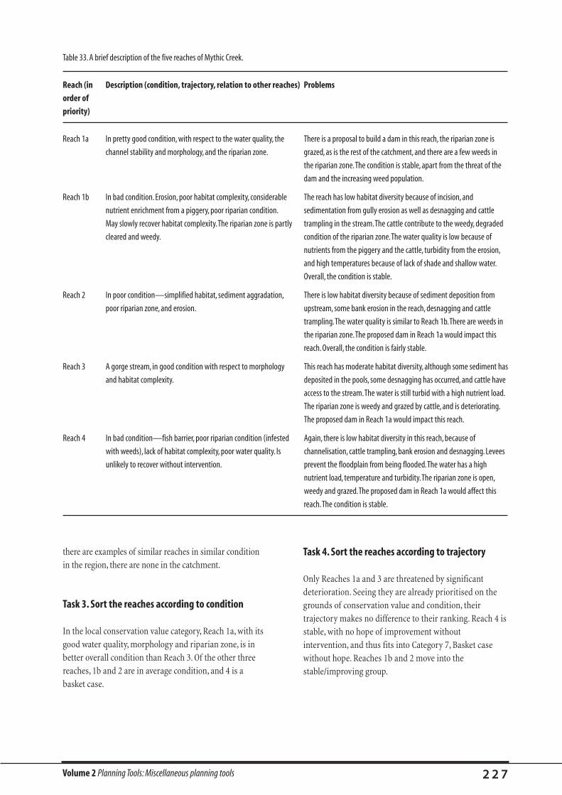
Volume 2 Planning Tools: Miscellaneous planning tools 2 2 7
there are examples of similar reaches in similar condition
in the region, there are none in the catchment.
Task 3. Sort the reaches according to condition
In the local conservation value category, Reach 1a, with its
good water quality, morphology and riparian zone, is in
better overall condition than Reach 3. Of the other three
reaches, 1b and 2 are in average condition, and 4 is a
basket case.
Task 4. Sort the reaches according to trajectory
Only Reaches 1a and 3 are threatened by significant
deterioration. Seeing they are already prioritised on the
grounds of conservation value and condition, their
trajectory makes no difference to their ranking. Reach 4 is
stable, with no hope of improvement without
intervention, and thus fits into Category 7, Basket case
without hope. Reaches 1b and 2 move into the
stable/improving group.
Table 33. A brief description of the five reaches of Mythic Creek.
Reach (in Description (condition, trajectory, relation to other reaches) Problems
order of
priority)
Reach 1a In pretty good condition, with respect to the water quality, the There is a proposal to build a dam in this reach, the riparian zone is
channel stability and morphology, and the riparian zone. grazed, as is the rest of the catchment, and there are a few weeds in
the riparian zone.The condition is stable, apart from the threat of the
dam and the increasing weed population.
Reach 1b In bad condition. Erosion, poor habitat complexity, considerable The reach has low habitat diversity because of incision, and
nutrient enrichment from a piggery, poor riparian condition. sedimentation from gully erosion as well as desnagging and cattle
May slowly recover habitat complexity.The riparian zone is partly trampling in the stream.The cattle contribute to the weedy, degraded
cleared and weedy. condition of the riparian zone.The water quality is low because of
nutrients from the piggery and the cattle, turbidity from the erosion,
and high temperatures because of lack of shade and shallow water.
Overall, the condition is stable.
Reach 2 In poor condition—simplified habitat, sediment aggradation, There is low habitat diversity because of sediment deposition from
poor riparian zone, and erosion. upstream, some bank erosion in the reach, desnagging and cattle
trampling.The water quality is similar to Reach 1b.There are weeds in
the riparian zone.The proposed dam in Reach 1a would impact this
reach. Overall, the condition is fairly stable.
Reach 3 A gorge stream, in good condition with respect to morphology This reach has moderate habitat diversity, although some sediment has
and habitat complexity. deposited in the pools, some desnagging has occurred, and cattle have
access to the stream.The water is still turbid with a high nutrient load.
The riparian zone is weedy and grazed by cattle, and is deteriorating.
The proposed dam in Reach 1a would impact this reach.
Reach 4 In bad condition—fish barrier, poor riparian condition (infested Again, there is low habitat diversity in this reach, because of
with weeds), lack of habitat complexity, poor water quality. Is channelisation, cattle trampling, bank erosion and desnagging. Levees
unlikely to recover without intervention. prevent the floodplain from being flooded.The water has a high
nutrient load, temperature and turbidity.The riparian zone is open,
weedy and grazed.The proposed dam in Reach 1a would affect this
reach.The condition is stable.
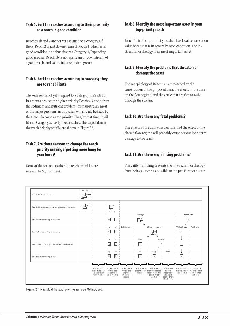
Volume 2 Planning Tools: Miscellaneous planning tools 2 2 8
Task 5. Sort the reaches according to their proximityto a reach in good condition
Reaches 1b and 2 are not yet assigned to a category. Of
these, Reach 2 is just downstream of Reach 1, which is in
good condition, and thus fits into Category 4, Expanding
good reaches. Reach 1b is not upstream or downstream of
a good reach, and so fits into the distant group.
Task 6. Sort the reaches according to how easy theyare to rehabilitate
The only reach not yet assigned to a category is Reach 1b.
In order to protect the higher priority Reaches 3 and 4 from
the sediment and nutrient problems from upstream, most
of the major problems in this reach will already be fixed by
the time it becomes a top priority. Thus, by that time, it will
fit into Category 5, Easily fixed reaches. The steps taken in
the reach priority shuffle are shown in Figure 36.
Task 7. Are there reasons to change the reachpriority rankings (getting more bang for your buck)?
None of the reasons to alter the reach priorities are
relevant to Mythic Creek.
Task 8. Identify the most important asset in yourtop-priority reach
Reach 1a is the top-priority reach. It has local conservation
value because it is in generally good condition. The in-
stream morphology is its most important asset.
Task 9. Identify the problems that threaten ordamage the asset
The morphology of Reach 1a is threatened by the
construction of the proposed dam, the effects of the dam
on the flow regime, and the cattle that are free to walk
through the stream.
Task 10. Are there any fatal problems?
The effects of the dam construction, and the effect of the
altered flow regime will probably cause serious long-term
damage to the reach.
Task 11. Are there any limiting problems?
The cattle trampling prevents the in-stream morphology
from being as close as possible to the pre-European state.
Task 1: Gather information
Unsorted
Deteriorating Without hope With hope
Close
Stable - Improving
Distant
Easy Hard
Average Basket case
Task 2: ID reaches with high conservation value assets
Task 3: Sort according to condition
Task 4: Sort according to trajectory
Task 5: Sort according to proximity to good reaches
Task 6: Sort according to ease
CATEGORY 1Protect regional
conservation value reaches
CATEGORY 2Protect local conservation value reaches
CATEGORY 3Protect and
improve deteriorating
reaches
CATEGORY 4Expand good
reaches
CATEGORY 5Improve impeded recovery reaches
(easily fixed reaches)
CATEGORY 6Improve
moderately damaged
reaches (more difficult to fix)
CATEGORY 7Improve basket case reaches
CATEGORY 8Improve basket case reaches
with hope
1b2
3
1b2
1b2
1b
1b
1b
2
4
4
4
4
2
2
1a
1a
1a
1a
1a
3
3
3
3
3
4
4
1a
Figure 36.The result of the reach priority shuffle on Mythic Creek.

Volume 2 Planning Tools: Miscellaneous planning tools 2 2 9
Task 12. Reshuffle the reach
The priorities so far are:
1. Stop the construction of the dam.
2. Exclude stock from the stream.
If we pretend these have been done, and reshuffle Reach
1a, where would it end up? It would return to Category 2,
Local conservation value, because of the relatively
untouched riparian vegetation. Once this was protected,
the reach would be reshuffled into the average condition
group, then into the stable to improving group, and finally
into Category 4, Expanding good assets. Reach 3 would
follow a similar path (Figure 37). The final list of problem
priorities for Mythic Creek can be found in Step 5 of the
Stream rehabilitation procedure, in Volume 1.
3.2. An example of the reshuffle in Simple Creek
Imagine Simple Creek, a small rural stream that can be
divided into two reaches.
1. The upstream reach is typical of many small streams in
the area. The riparian zone is in good condition.
However, for some years, the landowners have been
desnagging the reach, a process that is still continuing,
and erosion has caused a further loss of in-stream
habitat. The land use is changing from cropping to
grazing, and the riparian zone, bank structure and
water quality are all under threat from the impacts of
grazing. This reach is a Category 3, Deteriorating reach.
2. The downstream reach is stable, but generally in worse
condition. The riparian zone has been cleared and the
banks grazed for some time, and the damage has
already been done. However, a rare species of fish
persists in the pools. Because of this fish, the
downstream reach is a Category 1, Regional
conservation value reach.
We will now run through Tasks 8 to 13 twice.
Task 8. The most important asset in the top-priority
downstream reach is the rare fish.
Task 9. The fish population is threatened by a lack of
habitat for juvenile fish, because of the cattle trampling
and polluting the shallow areas. High water temperatures
in summer because of the lack of shade are another
problem.
Task 10. Neither problem is fatal.
Task 11. The lack of juvenile habitat is most limiting,
because it means only a few young fish survive each year.
The high summer temperatures are a stress on all the fish
but usually few die, so this is next most limiting.
Task 1: Gather information
Unsorted
Deteriorating Without hope
Close
Stable - Improving
Distant
Easy Hard Easy Hard
Average Basket caseBadGood
Task 2: ID reaches with high conservation value assets
Task 3: Sort according to condition
Task 4: Sort according to trajectory
Task 5: Sort according to proximity to good reaches
Task 6: Sort according to ease
CATEGORY 1Protect regional
conservation value reaches
CATEGORY 2Protect local conservation value reaches
CATEGORY 3Protect and
improve deteriorating
reaches
CATEGORY 4Expand good
reaches
CATEGORY 5Improve impeded recovery reaches
(easily fixed reaches)
CATEGORY 6Improve
moderately damaged
reaches (more difficult to fix)
CATEGORY 7Improve basket case reaches
CATEGORY 8Improve basket case reaches
with hope
CATEGORY 0Reaches in good
condition throughout, that
are already protected
With hope
3
1b2
1a
1b
1b
4
4
4
4
2
3 2
1a
1a
1a
1a
1a
3
3
3
3
3
1a
31a
1b2
31a
31a
Figure 37.The result of reshuffling Reaches 1a and 3 in Mythic Creek.

Volume 2 Planning Tools: Miscellaneous planning tools 2 3 0
Task 12. We now consider what category the downstream
reach would fit into if the rare fish were protected. The
reach has no other regional or local conservation assets,
and is not deteriorating, but it does have a good asset in
the rare fish. Thus, it would come out as Category 4, a reach
with good assets to be expanded on.
Task 13. We now repeat Tasks 8 to 13. However, now the
top priority is the upstream reach, because this is Category
3, and the downstream reach is Category 4.
Task 8. The most important asset in the upstream reach is
the riparian zone.
Task 9. The riparian zone is threatened by the impacts of
clearing and grazing.
Task 10. Clearing would be fatal to the riparian zone.
Task 11. Grazing in the riparian zone would be limiting.
Task 12. What category would this reach reshuffle into if
the riparian zone was protected from clearing and grazing?
Because of the desnagging that is continuing in this reach,
it would remain in Category 3, Deteriorating reaches. The
next iteration of tasks 8–13 would work out how to protect
the woody debris load from further deterioration.
Task 13. To finish working out the order in which
problems should be fixed, we would continue to repeat this
process, but this is enough to show you how the process
works. Below is a summary of the priorities for Simple
Creek that have come from the above prioritisation.
1. Protect the rare fish population in the downstream
reach by providing more juvenile habitat.
2. Protect the fish in the downstream reach by providing
shade to lower summer water temperatures.
3. Protect the riparian zone in the upstream reach by
preventing any clearing.
4. Protect the riparian zone in the upstream reach by
preventing grazing.
5. Protect the woody debris in the upstream reach
(individual problems not yet prioritised).
6. Improve the condition of the downstream reach
(individual problems not yet prioritised).
7. Improve the condition of the upstream reach
(individual problems not yet prioritised).

Volume 2 Planning Tools: Miscellaneous planning tools 2 3 1
The following tables summarise legislation relevant to
stream rehabilitation State by State. Unfortunately, tables
have not yet been developed for the ACT or the Northern
Territory. The table is designed to be used in Step 8: Are
your objectives feasible? in the Stream rehabilitation
procedure,Volume 1. The tables are set out as follows.
Column 1 Gives the issue: usually relating to ownership,
administration or specific management activities.
Column 2 Identifies the government agencies responsible for
administration of the issue.
Column 3 Lists the legislation and other documentation relevant to
the issue.
Column 4 Briefly discusses the issue.
Because legislation changes rapidly, and because your
situation may be unusual, we recommend that you verify your
legal position with the appropriate government department.
The following tables are provided as a guide only.
If you have any specific questions please contact the
person or department noted at the top of each table. The
information provided in these tables was distilled from
information provided by State government officers as
shown, and is considered a good guide as of 1998.
LEGISLATIVE AND ADMINISTRATIVECONSTRAINTS
1. Queensland stream management
Table 34. Legislation relevant to stream rehabilitation in Queensland.
Issue Agency Documentation Discussion
Administration:
Boundaries QDNR1 Water Resources Act 1989 Currently being reviewed by the Natural Resource Management Working Party (NRMWP). At
present the Crown maintains ownership of the bed up to the top of the low bank of the
watercourse. From a management perspective, a watercourse is interpreted as being land
between the high banks of any river, creek or stream which flows permanently or intermittently
through two or more properties.This is, however, applicable only to freshwater streams (down
to the tidal limit).The tidal limit is defined as the upstream extent of the ‘spring tide’.
Estuarine QDE2 Coastal Protection and For streams below the tidal limit, the Water Resources Act is no longer applicable, and
systems Management Act 1995 responsibility for most matters falls to the QDE, through the Coastal Protection Act and Nature
Nature Conservation Conservation Act. However, QDNR still has some jurisdiction by way of implementing the
Act 1992 Fisheries Act which applies to both fresh and saltwater systems.
By John Amprimo and Geoff Guinea*
The primary contact for all stream rehabilitation work in Queensland is the Department of Natural Resources (QDNR). Details of
relevant legislation are given in Table 34.
1 QDNR: Queensland Department of Natural Resources2 QDE: Queensland Department of Environment3 LGAQ: Local Government Association of Queensland
* Principal Advisers, Riverine Management, Queensland Department of Natural Resources, GPO Box 2454, Brisbane, Queensland 4001. Ph: (07) 3224 7668, Fax: (07) 3224 8359,
Email: [email protected]
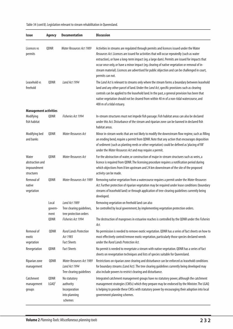
Volume 2 Planning Tools: Miscellaneous planning tools 2 3 2
Issue Agency Documentation Discussion
Licences vs QDNR Water Resources Act 1989 Activities in streams are regulated through permits and licences issued under the Water
permits Resources Act. Licences are issued for activities that will occur repeatedly (such as water
extraction), or have a long-term impact (eg. a large dam). Permits are issued for impacts that
occur once only, or have a minor impact (eg. clearing of native vegetation or removal of in-
stream material). Licences are advertised for public objection and can be challenged in court,
permits can not.
Leasehold vs QDNR Land Act 1994 The Land Act is relevant to streams only where the stream forms a boundary between leasehold
freehold land and any other parcel of land. Under the Land Act, specific provisions such as clearing
controls can be applied to the leasehold land. In the past, a general provision has been that
native vegetation should not be cleared from within 40 m of a non-tidal watercourse, and
400 m of a tidal estuary.
Management activities
Modifying QDNR Fisheries Act 1994 In-stream structures must not impede fish passage. Fish habitat areas can also be declared
fish habitat under this Act. Disturbance of the stream and riparian zone can be banned in declared fish
habitat areas.
Modifying bed QDNR Water Resources Act Minor in-stream works that are not likely to modify the downstream flow regime, such as filling
and banks an eroding bend, require a permit from QDNR. Note that any action that encourages deposition
of sediment (such as planting reeds or other vegetation) could be defined as ‘placing of fill’
under the Water Resources Act and may require a permit.
Water QDNR Water Resources Act For the abstraction of water, or construction of major in-stream structures such as weirs, a
abstraction and licence is required from QDNR.The licensing procedure requires a notification period during
impoundment which objections from 8 km upstream and 24 km downstream of the site of the proposed
structures activity can be made.
Removal of QDNR Water Resources Act 1989 Removing native vegetation from a watercourse requires a permit under the Water Resources
native Act. Further protection of riparian vegetation may be required under lease conditions (boundary
vegetation streams of leasehold land) or through application of tree-clearing guidelines currently being
developed.
Local Land Act 1989 Removing vegetation on freehold land can also
govern- Tree clearing guidelines, be controlled by local government, by implementing vegetation protection orders.
ment tree protection orders
QDNR Fisheries Act 1994 The destruction of mangroves in estuarine reaches is controlled by the QDNR under the Fisheries
Act.
Removal of QDNR Rural Lands Protection No permission is needed to remove exotic vegetation. QDNR has a series of fact sheets on how to
exotic Act 1985 most effectively control/remove exotic vegetation, particularly those species declared weeds
vegetation Fact Sheets under the Rural Lands Protection Act.
Revegetation QDNR Fact Sheets No permit is needed to revegetate a stream with native vegetation. QDNR has a series of fact
sheets on revegetation techniques and lists of species suitable for Queensland.
Riparian zone QDNR Water Resources Act 1989 Restrictions on riparian zone clearing and disturbance can be enforced as leasehold conditions
management Land Act 1994 for boundary streams (Land Act). The tree clearing guidelines currently being developed may
Tree clearing guidelines also include powers to restrict clearing and disturbance.
Catchment QDNR No statutory Integrated catchment management groups have no statutory power, although the catchment
management LGAQ3 authority management strategies (CMSs) which they prepare may be endorsed by the Minister.The LGAQ
groups Incorporation is helping to provide these CMSs with statutory power by encouraging their adoption into local
into planning government planning schemes.
schemes
Table 34 (cont’d). Legislation relevant to stream rehabilitation in Queensland.
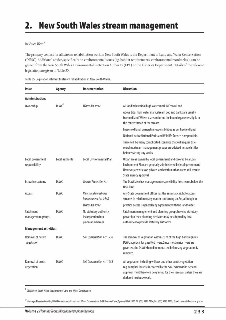
Table 35. Legislation relevant to stream rehabilitation in New South Wales.
Issue Agency Documentation Discussion
Administration:
Ownership DLWC1
Water Act 1912 All land below tidal high water mark is Crown Land.
Above tidal high water mark, stream bed and banks are usually
freehold land.Where a stream forms the boundary, ownership is to
the centre thread of the stream.
Leasehold land: ownership responsibilities as per freehold land.
National parks: National Parks and Wildlife Service is responsible.
There will be many complicated scenarios that will require title
searches: stream management groups are advised to search titles
before starting any works.
Local government Local authority Local Environmental Plan Urban areas owned by local government and covered by a Local
responsibility Environment Plan are generally administered by local government.
However, activities on private lands within urban areas still require
State agency approval.
Estuarine systems DLWC Coastal Protection Act The DLWC also has management responsibility for streams below the
tidal limit.
Access DLWC Rivers and Foreshores Any State government officer has the automatic right to access
Improvement Act 1948 streams in relation to any matter concerning an Act, although in
Water Act 1912 practice access is generally by agreement with the landholder.
Catchment DLWC No statutory authority Catchment management and planning groups have no statutory
management groups Incorporation into power but their planning decisions may be adopted by local
planning schemes authorities to provide statutory authority.
Management activities:
Removal of native DLWC Soil Conservation Act 1938 The removal of vegetation within 20 m of the high bank requires
vegetation DLWC approval for gazetted rivers. Since most major rivers are
gazetted, the DLWC should be contacted before any vegetation is
removed.
Removal of exotic DLWC Soil Conservation Act 1938 All vegetation including willows and other exotic vegetation
vegetation (eg. camphor laurels) is covered by the Soil Conservation Act and
approval must therefore be granted for their removal unless they are
declared noxious weeds.
Volume 2 Planning Tools: Miscellaneous planning tools 2 3 3
2. New South Wales stream management
by Peter Wem*
The primary contact for all stream rehabilitation work in New South Wales is the Department of Land and Water Conservation
(DLWC). Additional advice, specifically on environmental issues (eg. habitat requirements, environmental monitoring), can be
gained from the New South Wales Environmental Protection Authority (EPA) or the Fisheries Department. Details of the relevent
legislation are given in Table 35.
1 DLWC: New South Wales Department of Land and Water Conservation
* Manager,Riverine Corridor, NSW Department of Land and Water Conservation, 2-24 Rawson Place, Sydney, NSW 2000. Ph: (02) 9372 7724, Fax: (02) 9372 7799, Email: [email protected]
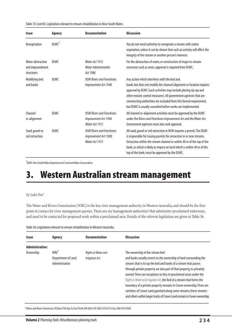
Volume 2 Planning Tools: Miscellaneous planning tools 2 3 4
Issue Agency Documentation Discussion
Revegetation DLWC1 You do not need authority to revegetate a stream with native
vegetation, unless it can be shown that such an activity will affect the
integrity of the stream or another person’s interests.
Water abstraction DLWC Water Act 1912 For the abstraction of water, or construction of major in-stream
and impoundment Water Administration structures such as weirs, approval is required from DLWC.
structures Act 1986
Modifying bed DLWC NSW Rivers and Foreshores Any action which interferes with the bed and
and banks Improvement Act 1948 banks but does not modify the channel alignment or location requires
approval by DLWC (such activities may include placing rip rap and
other erosion control measures). All government agencies that are
constructing authorities are excluded from this formal requirement,
but DLWC is usually consulted before works are implemented.
Channel DLWC NSW Rivers and Foreshores All channel re-alignment activities must be approved by the DLWC
re-alignment Improvement Act 1948 under the Rivers and Foreshores Improvement Act and the Water Act.
Water Act 1912 Government agencies must also seek approval.
Sand, gravel or DLWC NSW Rivers and Foreshores All sand, gravel or soil extraction in NSW requires a permit.The DLWC
soil extraction Improvement Act 1948; is responsible for issuing permits for extraction in or near streams.
Water Act 1912 Extraction within the stream channel or within 40 m of the top of the
bank, or which is likely to impact on land which is within 40 m of the
top of the bank, must be approved by the DLWC.
1DLWC: New South Wales Department of Land and Water Conservation
Table 36. Legislation relevant to stream rehabilitation in Western Australia.
Issue Agency Documentation Discussion
Administration:
Ownership WRC1 Rights in Water and The ownership of the stream bed
Department of Land Irrigation Act and banks usually reverts to the ownership of land surrounding the
Administration stream; that is to say the bed and banks of a stream that passes
through private property are also part of that property, ie. privately
owned.There are exceptions to this; in proclaimed areas under the
Rights in Water and Irrigation Act, the bed of a stream that forms the
boundary of a private property remains in Crown ownership.There are
corridors of Crown Land gazetted along some streams; these streams
and others within larger tracks of Crown Land remain in Crown ownership.
3. Western Australian stream management
by Luke Pen*
The Water and Rivers Commission (WRC) is the key river management authority in Western Australia, and should be the first
point of contact for river management queries. There are six ‘management authorities’ that administer proclaimed waterways,
and need to be contacted for proposed work within a proclaimed area. Details of the relevent legislation are given in Table 36.
* Water and Rivers Commision, PO Box 6740 Hay St, East Perth,WA 6892. Ph: (08) 9278 0374, Fax: (08) 9278 0585
Table 35 (cont’d). Legislation relevant to stream rehabilitation in New South Wales.
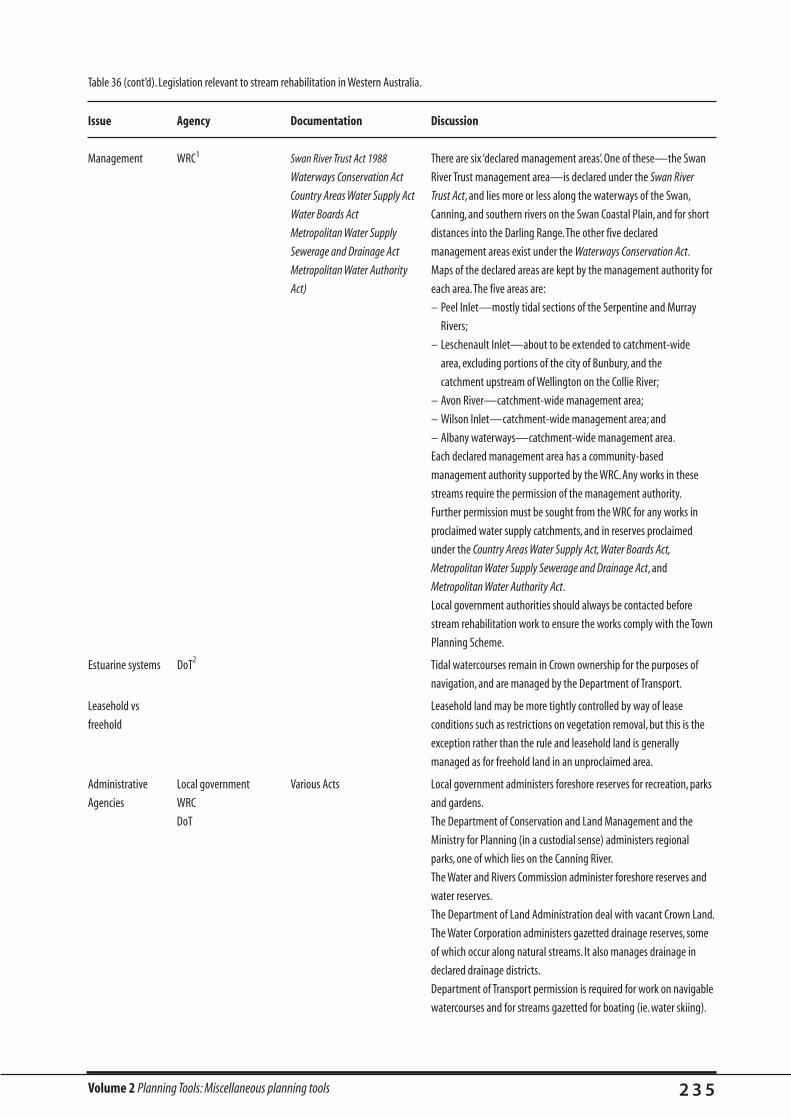
Volume 2 Planning Tools: Miscellaneous planning tools 2 3 5
Issue Agency Documentation Discussion
Management WRC1 Swan River Trust Act 1988 There are six ‘declared management areas’. One of these—the Swan
Waterways Conservation Act River Trust management area—is declared under the Swan River
Country Areas Water Supply Act Trust Act, and lies more or less along the waterways of the Swan,
Water Boards Act Canning, and southern rivers on the Swan Coastal Plain, and for short
Metropolitan Water Supply distances into the Darling Range.The other five declared
Sewerage and Drainage Act management areas exist under the Waterways Conservation Act.
Metropolitan Water Authority Maps of the declared areas are kept by the management authority for
Act) each area.The five areas are:
– Peel Inlet—mostly tidal sections of the Serpentine and Murray
Rivers;
– Leschenault Inlet—about to be extended to catchment-wide
area, excluding portions of the city of Bunbury, and the
catchment upstream of Wellington on the Collie River;
– Avon River—catchment-wide management area;
– Wilson Inlet—catchment-wide management area; and
– Albany waterways—catchment-wide management area.
Each declared management area has a community-based
management authority supported by the WRC. Any works in these
streams require the permission of the management authority.
Further permission must be sought from the WRC for any works in
proclaimed water supply catchments, and in reserves proclaimed
under the Country Areas Water Supply Act,Water Boards Act,
Metropolitan Water Supply Sewerage and Drainage Act, and
Metropolitan Water Authority Act.
Local government authorities should always be contacted before
stream rehabilitation work to ensure the works comply with the Town
Planning Scheme.
Estuarine systems DoT2 Tidal watercourses remain in Crown ownership for the purposes of
navigation, and are managed by the Department of Transport.
Leasehold vs Leasehold land may be more tightly controlled by way of lease
freehold conditions such as restrictions on vegetation removal, but this is the
exception rather than the rule and leasehold land is generally
managed as for freehold land in an unproclaimed area.
Administrative Local government Various Acts Local government administers foreshore reserves for recreation, parks
Agencies WRC and gardens.
DoT The Department of Conservation and Land Management and the
Ministry for Planning (in a custodial sense) administers regional
parks, one of which lies on the Canning River.
The Water and Rivers Commission administer foreshore reserves and
water reserves.
The Department of Land Administration deal with vacant Crown Land.
The Water Corporation administers gazetted drainage reserves, some
of which occur along natural streams. It also manages drainage in
declared drainage districts.
Department of Transport permission is required for work on navigable
watercourses and for streams gazetted for boating (ie. water skiing).
Table 36 (cont’d). Legislation relevant to stream rehabilitation in Western Australia.
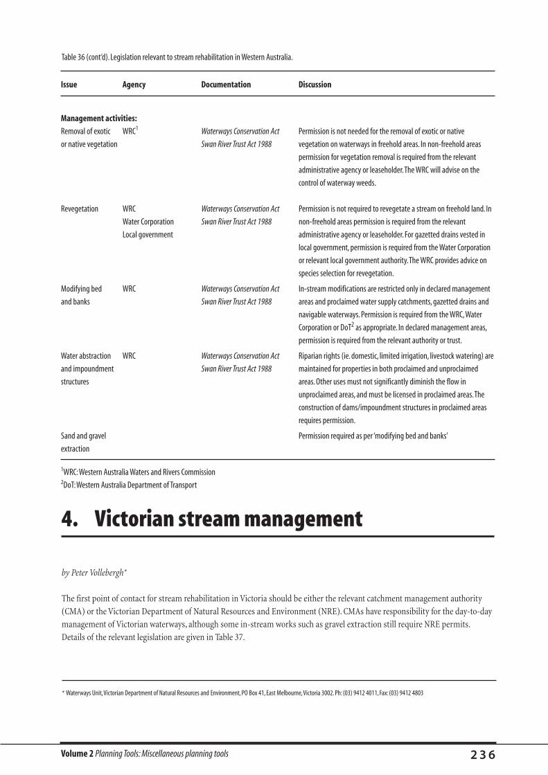
Volume 2 Planning Tools: Miscellaneous planning tools 2 3 6
Issue Agency Documentation Discussion
Management activities:
Removal of exotic WRC1 Waterways Conservation Act Permission is not needed for the removal of exotic or native
or native vegetation Swan River Trust Act 1988 vegetation on waterways in freehold areas. In non-freehold areas
permission for vegetation removal is required from the relevant
administrative agency or leaseholder.The WRC will advise on the
control of waterway weeds.
Revegetation WRC Waterways Conservation Act Permission is not required to revegetate a stream on freehold land. In
Water Corporation Swan River Trust Act 1988 non-freehold areas permission is required from the relevant
Local government administrative agency or leaseholder. For gazetted drains vested in
local government, permission is required from the Water Corporation
or relevant local government authority.The WRC provides advice on
species selection for revegetation.
Modifying bed WRC Waterways Conservation Act In-stream modifications are restricted only in declared management
and banks Swan River Trust Act 1988 areas and proclaimed water supply catchments, gazetted drains and
navigable waterways. Permission is required from the WRC,Water
Corporation or DoT2 as appropriate. In declared management areas,
permission is required from the relevant authority or trust.
Water abstraction WRC Waterways Conservation Act Riparian rights (ie. domestic, limited irrigation, livestock watering) are
and impoundment Swan River Trust Act 1988 maintained for properties in both proclaimed and unproclaimed
structures areas. Other uses must not significantly diminish the flow in
unproclaimed areas, and must be licensed in proclaimed areas.The
construction of dams/impoundment structures in proclaimed areas
requires permission.
Sand and gravel Permission required as per ‘modifying bed and banks’
extraction
1WRC:Western Australia Waters and Rivers Commission2DoT:Western Australia Department of Transport
4. Victorian stream management
by Peter Vollebergh*
The first point of contact for stream rehabilitation in Victoria should be either the relevant catchment management authority
(CMA) or the Victorian Department of Natural Resources and Environment (NRE). CMAs have responsibility for the day-to-day
management of Victorian waterways, although some in-stream works such as gravel extraction still require NRE permits.
Details of the relevant legislation are given in Table 37.
Table 36 (cont’d). Legislation relevant to stream rehabilitation in Western Australia.
* Waterways Unit,Victorian Department of Natural Resources and Environment, PO Box 41, East Melbourne,Victoria 3002. Ph: (03) 9412 4011, Fax: (03) 9412 4803

Volume 2 Planning Tools: Miscellaneous planning tools 2 3 7
Table 37. Legislation relevant to stream rehabilitation in Victoria.
Issue Agency Documentation Discussion
Administration:
Ownership NRE1, CMAs2 Land Act 1958 Bed and banks in Victorian streams are usually the property of the
Crown (some that were alienated early are privately owned, eg. part of
the western district).
On larger streams there is usually Crown Land frontage.This comprises
a Crown reserve extending back 20 m from the top of each bank, plus
a variable width of ‘unreserved’Crown Land between the reserve and
the surveyed boundary.There are 25,000 km of frontage reserves.
Frontage reserves are static, so if the stream course changes, the public
reserve can become landlocked in private farmland.Stock grazing on
public water frontages has been permitted via agricultural licences
issued by NRE.The power to issue these licences will be transferred to
CMAs in early to mid 1999.
The first point of contact on administrative matters should be either
the relevant CMA or the NRE. CMAs have responsibility for the day-to-
day management of Victorian waterways, although some in-stream
works such as gravel extraction still require NRE permits.
Administration of NRE, CMAs, local Water Act 1989 Crown frontage is administered by NRE or CMAs via licence conditions
bed and banks governments Planning and Environment covering its use.
Act 1987 Private frontage may be controlled by local government planning
scheme requirements.
Estuarine systems CMA, port authorities Water Act 1989 A waterway includes intermittently and permanently flowing creeks,
Marine Act 1988 rivers, streams and watercourses. (This presumably includes estuarine
Port of Melbourne Authority reaches.) The lower reaches of the Gippsland Lakes Rivers, Snowy
Act 1958 River, Lower Genoa River , Corner Inlet etc. are designated as ports
under the Marine Act 1988 and Port of Melbourne Authority Act 1958.
The appropriate port authority must be contacted for any works in
these areas.
Heritage rivers CMA Heritage Rivers Act 1992 Eighteen rivers are declared as heritage rivers because of their natural,
and PV3 within cultural, heritage, recreational and scenic values.Works around these
National Parks rivers must be in accord with the management plans and other
heritage river recommendations.
Access Land Act 1958 Public access is permitted to Crown frontages for recreation (not
including camping), but access to Crown frontages cannot be
obtained through private land without the landowner’s consent.
CMA NRE Water Act 1989 CMAs have statutory power under the Water Act.The responsibility for
day-to-day stream management issues is delegated from NRE to the
CMAs. CMAs have the capacity to make by-laws to control activities on
waterways.
Management activities:
Removal of native CMA State section of the Remnant vegetation cannot be removed within 30 m of a
vegetation planning scheme waterway. Also, native vegetation on any landholding of 0.4 ha or
greater cannot be destroyed or lopped. Complete details are in
‘Planning guidelines for native vegetation retention controls’,
available through NRE.

Volume 2 Planning Tools: Miscellaneous planning tools 2 3 8
Issue Agency Documentation Discussion
Removal of exotic CMA Water Act 1989 The removal of exotic vegetation (excluding those classified as
vegetation noxious weeds under Catchment and Land Protection Act 1994) from
a waterway requires a ‘works on waterway’ permit from the relevant
CMA.
Revegetation CMA You do not need authority to revegetate a stream using native
vegetation. CMA offices can provide advice on revegetation.
Modifying the NRE Flora and Fauna Guarantee A permit from NRE is required for undertaking any works
riparian zone habitat Act 1988 where taxa listed under the Flora and Fauna Guarantee Act are likely
to be killed, injured, disturbed or collected. Management actions also
have to be compatible with action plans currently being prepared
(under the Flora and Fauna Act 1988) to counter the following
potentially threatening processes:
– removal of woody debris from Victorian streams;
– increase in sediment input to rivers and streams due to human
activities;
– the prevention of passage of aquatic biota as a result of the
presence of in-stream structures;
– degradation of native riparian vegetation along Victoria’s rivers and
streams;
– deliberate or accidental introduction of live fish into public or
private waters within a Victorian river catchment, when the taxon
to which the fish belongs cannot reliably be inferred to have been
present before 1770; and
– alteration to the natural temperature regimes of rivers and streams.
Water abstraction NRE, rural water Conservation, Forests and The construction of dams, weirs, or other structures, in or across
and impoundment authorities Lands Act 1987 waterways which potentially interfere with the passage of fish or the
structures Water Act 1989 quality of aquatic habitat must be submitted to NRE for comment.
Approvals are required from the relevant rural water authority
(Goulburn Murray Water, Southern Rural Water,Wimmera Mallee
Water, Sunraysia Rural Water).
Modifying bed and NRE Water Act 1989 Any modification of the waterway, including stream stabilisation
banks or channel works, requires a ‘works on waterways’ permit from NRE.
re-alignment
Sand, gravel or NRE Extractive Industries Large-scale extraction operations >2,000 m2 and >2 m depth need a
soil extraction Development Act 1995 licence under the Extractive Industries Development Act. Most river
Land Act 1958 sand and gravel extraction operations are smaller than this.
Catchment and Land Small-scale extraction operations on Crown Land require a licence
Protection Act 1994 issued by NRE under the Land Act (or occasionally the Forests Act).
Water Act 1989 Small-scale extraction on private land requires authorisation by NRE
under part 7 of the Catchment and Land Protection Act.
All sand and gravel extractions on waterways also require a ‘works on
waterways’ permit from NRE.
Further information can be found in ‘Extractive Industries on Crown
Land. Owners Consent. Guidelines on Issues and Processes’, available
from NRE.
1NRE:Victoria Department of Natural Resources and Environment2CMA: Catchment Management Authority3PV: Parks Victoria
Table 37 (cont’d). Legislation relevant to stream rehabilitation in Victoria.

Volume 2 Planning Tools: Miscellaneous planning tools 2 3 9
5. South Australian stream management
by Jim Burston*
Stream management in South Australia is delegated to catchment water management boards and local government. The
Department of Environment and Natural Resources (DENR) can provide advice on whether there is a management board for
your particular stream.Details of the relevant legislation are given in Table 38.
Table 38. Legislation relevant to stream rehabilitation in South Australia.
Issue Agency Documentation Discussion
Administration:
Ownership Land Act 1958 The ownership of the bed and banks of a stream usually reverts to the
ownership of the surrounding land.This means that river frontage
reserves are not usually specified except in urban areas where
watercourses have the status of ‘reserve’ and are managed by local
government.
Administration CWMB1 Water Resources Act 1997 Watercourses are termed ‘prescribed’ or ‘non-prescribed’. A prescribed
WRPC2 watercourse is one where water extraction must be authorised.
Local government The management of streams is delegated to four authorities based on
DENR3 the preparation of water plans:
• State Water Management Plans are administered by WRPC;
• Catchment Water Management Plans are administered by the CWMB;
• Local Water Management Plans are administered by local
government. Streams within local government boundaries are
administered by the local government; and
• Watercourses outside local government boundaries that are not
covered by any of the above water plans are administered by DENR.
There are water plans for the River Torrens and Patawalonga
catchments. Plans are expected to be adopted for the Onkaparinga
River, Murray River and North Adelaide–Barossa catchments by
June 1999.
Access CWMB Water Resources Act 1997 Where the watercourse is on private land, permission to enter a
property should be obtained from the landholder, although
authorised officers under the Water Resources Act may enter any land.
General duty of Environmental Protection Act 1993 All management activities need to take account of Section 25 of the
care Water Resources Act 1997 Environmental Protection Act, which relates to general environmental
duty.
Under the Water Resources Act,
• landholders are obliged to maintain their watercourse(s) in good
condition; and
• landholders have a duty to take reasonable steps to prevent damage
to the bed and banks of a watercourse.
* South Australian Department for Environment, Heritage and Aboriginal Affairs, GPO Box 1047, Adelaide, SA 5001. Ph: (08) 8204 9108, Fax: (08)8204 9144, Email: [email protected]

Volume 2 Planning Tools: Miscellaneous planning tools 2 4 0
Issue Agency Documentation Discussion
Management activities:
Removal of native Native Vegetation Council Native Vegetation Act 1991 Permission is required for the removal or clearance of all native
vegetation riparian vegetation, both aquatic and terrestrial.
Removal of exotic DENR, CWMB or local Local Government Act 1934 Exotic vegetation removal must comply with any water plan covering
vegetation council the site.
Animal and Plant Control Local government may remove obstructions, so if willows are
(Agricultural Protection and obstructing the channel, local government can give approval for their
Other Purposes) Act 1986 removal.
Landholders have an obligation to destroy vegetation defined under
S.57 of the Animal and Plant Control Act.
Revegetation Local Government Act 1997, No permission is required to fence and revegetate along a channel.
S.636 & 641 However, if the revegetation causes any ‘obstruction’ or may cause
flooding that will be a danger to life or property, the local
government may remove the obstruction.
Water abstraction CWMB1 or DENR3, Water Resources Act 1997 For prescribed watercourses under the Water Resources Act,
and impoundment Local government S.9(3)(e) & S.9(4)(a) permission is required to abstract water.
structures Local Government Act 1934 S.635 Advice on prescribed watercourses can be obtained from the relevant
Development Act 1993 contact agency for your stream,ie.WRPC2,CWMB,local government,DENR.
For non-prescribed watercourses, abstraction is acceptable as long as
it does not contravene a water plan.
For impoundment structures, a permit to undertake a ‘water affecting
activity’ must be obtained from DENR, unless that activity constitutes
a ‘development’ for the purposes of the Development Act. However,
such development activities are referred to the DENR as part of the
planning process.
Modifying bed DENR; CWMB or local Water Resources Act 1997, S9 Where a water plan exists, permission is required from the relevant
and banks government; EPA4 Local Government Act, S.635 contact agency, ie. CWMB, local government , DENR.
Environmental Protection Additional permission may be required from the local council as well
Act 1993 S.25 as from the CWMB or DENR.
If the works may contribute to the release of sediment such that the
sediment load exceeds 25 mg per litre suspended load, then a licence
is required from the EPA.
All works should confirm to the EPA’s Stormwater Pollution Control
Code of Practice.
Sand, gravel or soil CWMB, DENR, and Water Resources Act 1997, S.9 Where a water plan exists, permission is required from the relevant
extraction local government Local Government Act 1934,S.635 contact agency, ie. CWMB, local government , DENR.
Additional permission is also required from the local government
authority.
1CWMB: Catchment Water Management Board
2WRPC:Water Resources Planning Committee
3DENR: South Australia Department of Environment and Natural Resources
4EPA: Environmental Protection Authority
Table 38 (cont’d). Legislation relevant to stream rehabilitation in South Australia.
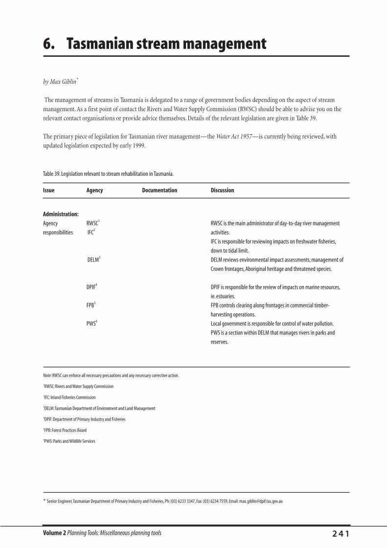
Volume 2 Planning Tools: Miscellaneous planning tools 2 4 1
6. Tasmanian stream management
by Max Giblin*
The management of streams in Tasmania is delegated to a range of government bodies depending on the aspect of stream
management. As a first point of contact the Rivers and Water Supply Commission (RWSC) should be able to advise you on the
relevant contact organisations or provide advice themselves. Details of the relevant legislation are given in Table 39.
The primary piece of legislation for Tasmanian river management—the Water Act 1957—is currently being reviewed, with
updated legislation expected by early 1999.
Table 39. Legislation relevant to stream rehabilitation in Tasmania.
Issue Agency Documentation Discussion
Administration:
Agency RWSC1 RWSC is the main administrator of day-to-day river management
responsibilities IFC2 activities.
IFC is responsible for reviewing impacts on freshwater fisheries,
down to tidal limit.
DELM3 DELM reviews environmental impact assessments; management of
Crown frontages, Aboriginal heritage and threatened species.
DPIF4 DPIF is responsible for the review of impacts on marine resources,
ie. estuaries.
FPB5 FPB controls clearing along frontages in commercial timber-
harvesting operations.
PWS6 Local government is responsible for control of water pollution.
PWS is a section within DELM that manages rivers in parks and
reserves.
Note: RWSC can enforce all necessary precautions and any necessary corrective action.
1RWSC: Rivers and Water Supply Commission
2IFC: Inland Fisheries Commission
3DELM:Tasmanian Department of Environment and Land Management
4DPIF: Department of Primary Industry and Fisheries
5FPB: Forest Practices Board
6PWS: Parks and Wildlife Services
* Senior Engineer,Tasmanian Department of Primary Industry and Fisheries, Ph: (03) 6233 3347, Fax: (03) 6234 7559, Email: [email protected]
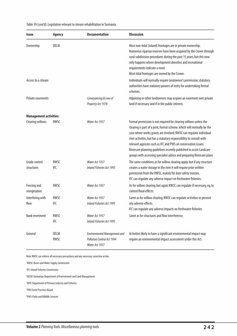
Volume 2 Planning Tools: Miscellaneous planning tools 2 4 2
Issue Agency Documentation Discussion
Ownership DELM Most non-tidal (inland) frontages are in private ownership.
Numerous riparian reserves have been acquired by the Crown through
rural subdivision procedures during the past 15 years, but this now
only happens where development densities and recreational
requirements indicate a need.
Most tidal frontages are owned by the Crown.
Access to a stream Individuals will normally require landowner’s permission; statutory
authorities have statutory powers of entry for undertaking formal
schemes.
Private easements Conveyancing & Law of Adjoining or other landowners may acquire an easement over private
Property Act 1978 land if necessary and if in the public interest.
Management activities:
Clearing willows RWSC Water Act 1957 Formal permission is not required for clearing willows unless the
clearing is part of a joint, formal scheme, which will normally be the
case where works grants are involved. RWSC can regulate individual
river activities, but has a statutory responsibility to consult with
relevant agencies such as IFC and PWS on conservation issues.
Rivercare planning guidelines recently published to assist Landcare
groups with accessing specialist advice and preparing Rivercare plans
Grade control RWSC Water Act 1957 The same conditions as for willow clearing apply; but if any structure
structures IFC Inland Fisheries Act 1995 creates a water storage in the river it will require prior written
permission from the RWSC, mainly for dam safety reasons.
IFC can regulate any adverse impact on freshwater fisheries.
Fencing and RWSC Water Act 1957 As for willow clearing; but again RWSC can regulate if necessary, eg. to
revegetation control flood effects.
Interfering with RWSC Water Act 1957 Same as for willow clearing; RWSC can regulate activities to prevent
flow IFC Inland Fisheries Act 1995 any adverse effects.
IFC can regulate any adverse impacts on freshwater fisheries
Bank revetment RWSC Water Act 1957 Same as for structures and flow interference.
IFC Inland Fisheries Act 1995
General DELM Environmental Management and Activities likely to have a significant environmental impact may
RWSC Pollution Control Act 1994 require an environmental impact assessment under this Act.
Water Act 1957
Note: RWSC can enforce all necessary precautions and any necessary corrective action.
1RWSC: Rivers and Water Supply Commission
2IFC: Inland Fisheries Commission
3DELM:Tasmanian Department of Environment and Land Management
4DPIF: Department of Primary Industry and Fisheries
5FPB: Forest Practices Board
6PWS: Parks and Wildlife Services
Table 39 (cont’d). Legislation relevant to stream rehabilitation in Tasmania.

dollar terms (present value) and simply sum the present
value of the costs and benefits to get the net present value
(NPV) of the project.
A difficulty of BCA is that, in trying to convert future
dollars to a current value, we often need to predict what the
future value will be (eg. what if land has been lost to
erosion in 10 years time; what will be the cost of land ten
years from now?) then discount the future value to give it a
present value. Economics textbooks such as that of Hanley
and Splash (1993) explain how to select the appropriate
discount rate and calculate present values.
This section describes BCA for stream rehabilitation
projects, and concludes that it is difficult to apply
traditional BCA to stream rehabilitation because of the
many non-market benefits involved, although the rapid
appraisal method (RAM) provides some techniques for
valuing such benefits. For details of the methods
summarised here see Read Sturgess & Associates (1992).
Two case studies of BCA are included at the end of the
section. One, from north-east Victoria, using the RAM
approach, and one from Queensland, using standard BCA.
Volume 2 Planning Tools: Miscellaneous planning tools 2 4 3
Produced from material provided by Mike Read and Neil
Sturgess*
Benefit–cost analysis (BCA) is used to help make
government and community decisions about whether to
spend scarce public funds on, say, river management
rather than on other investments, or the decision about
which river management programs represent the best use
of scarce funds (Read Sturgess & Associates, 1992). The
assumption is that the best value project will return the
highest benefit for a given cost. BCA is a method that
applies a strict procedure to produce this ratio of benefits
to costs.
BCA is simply a process of comparing all the cost and
benefits of a particular project in current dollar terms. For
example, a rehabilitation strategy might be to remove
willows from a stream in year one, fence the stream in year
two, and revegetate the stream in year four. The benefit of
this project may be a pick up in the recreational fishing
industry in the stream from year 10 onward. So how do we
compare the costs which are expended in the first few
years with benefits which don’t start for 10 years? The
solution is to convert all costs and benefits to current
BENEFIT–COST ANALYSIS OF STREAMREHABILITATION PROJECTS
BCA is excellent for assessing the value of projects with a
financial return and involving commodities that can be
given a price based on market values. For example,
consider a proposal to build a dam that will supply
irrigation water. The cost of the dam, reticulation and land
lost due to inundation can all be given market values, as
can the expected increase in returns (benefits) through the
use of water for irrigation. Thus, a BCA of the market
goods (those goods which are tradeable and hence have a
market value) is relatively easy to make. BCA of projects
dominated by non-market goods is not so easy. The non-
market goods are those which are not traded. They include
items such as the value of pristine wilderness, and the
value of being able to use the river or dam for recreation.
All stream rehabilitation projects will have a large
proportion of non-market values driving them.
Unfortunately, it is generally much easier to justify the
environmental destruction of a stream with a BCA than it
is to justify the stream’s rehabilitation. There are three
reasons for this.
1. As we have emphasised many times, it costs much
more to fix a stream than to destroy it. This is largely
because the human impact on stream systems often
induces an increase of energy. That is, channelisation,
gullying, levees etc. all lead to an increase in the ‘power’
of a stream system (increased slope or increased
1. The difficulty of applying BCA
* Read Sturgess and Associates, 89 Gladstone St, Kew,Victoria 3101. Ph: (03) 9853 2929, Fax: (03) 9853 0205, Email: [email protected]

Volume 2 Planning Tools: Miscellaneous planning tools 2 4 4
discharge). Rehabilitation efforts have to overcome this
energy and so are expensive.
2. Estimating the benefits and costs requires an
assessment of the probability of particular changes
occurring in the stream if the works are not done. For
example, what will be the cost of increased suspended
loads to streams if work is not done? ‘What if ’
questions of this type are inherently difficult to answer.
3. The benefits of the stream rehabilitation are usually
non-market benefits and therefore difficult to cost.
The difficulty in conducting BCA for ‘environmental’
stream projects is that of establishing the costs and
benefits of the non-market values they are concerned with,
such as people’s desire to enjoy spending time in natural
surroundings, or the value of a slightly degraded
environment as compared with a pristine one?
A recent alternative to BCA for assessing the value of
projects with many non-market values is multi-criteria
analysis (MCA). This compares projects dominated by
non-market goods by ‘scoring’ the non-market goods.
Some people see MCA as an acceptable alternative to BCA
and a panacea for decision analysis. Reed and Sturgess
strongly disagree, saying that MCA merely shifts the hard
part of the analysis from the question of valuing unpriced
goods and services to deciding on what weights to give the
criteria that are used to score those goods and services.
Those weights had better be proportional to the
community’s willingness to pay for the goods and services
(what is assessed for BCA) or MCA will give the wrong
answer. Furthermore, as well as the river engineer, MCA
needs a team of technical experts if it is to be done
properly, BCA needs a single, determined economist. In the
end, both provide information to the decision-makers but
decision-makers must still exercise their interpretive skills
and their judgment.
BCA remains the standard procedure for valuing projects,
is widely accepted by government treasuries and program
administrators, and is the standard adopted by the OECD
and the Commonwealth Government and the
Murray–Darling Basin Commission.
Information that isuseful for BCAAt first it might appear remarkable how little information is
available on the benefits that accrue from stream
rehabilitation activities.The surprise may diminish when one
tries to measure the subtle effects of various treatments.The
following evaluation of a gully control project shows clearly
that rehabilitation work can be cost effective.
Sharpley et al. (1996) reported on a 13-year study of the effects
of treating a 5.7 ha gullied catchment by bulldozing the gullies
(gully shaping) and seeding with Bermuda grass.The gullied
catchment lost 27,500 kg of soil, 7.1 kg N, and 4.1 kg of
P/ha/year, compared with the ungullied control catchment
that lost 4,900 kg of sediment, 3.1 kg N, and 1.6 kg of
P/ha/year.The cost of the treatment was $US1,100/ha, which
means that 210 kg of sediment, 5 g N and 3 g P were retained for every
dollar spent on treatment.
These results provide a strong case for use of BCA in planning
stream rehabilitation work.
There are three basic methods of valuing non-market
goods. BCA textbooks, such as that of Hanley and Splash
(1993), can be consulted for further details of their
application and limitations.
1. The hedonic pricing method (HP) links the value of the
non-market good to that of a market good (Hanley and
Spash, 1993). For example, a farm containing a ‘natural’
stream may have a higher value than a farm with a
degraded stream (other factors being equal). Thus, by
improving the degraded stream to a ‘natural’ state will
increase the market value of a farm.
2. The contingent valuation method (CVM) estimates
market values through willingness to pay (WTP) and
willingness to receive. For example, improved stream
2. How to value non-market goods
Volume 2 Planning Tools: Miscellaneous planning tools 2 4 5
habitat brought about by stream rehabilitation could be
valued by asking stream users how much they are
willing to pay for improved habitat. How much, for
instance, would visitors be willing to pay for the
improved fishing following stream rehabilitation?
3. The travel cost method: is based on the expense users
actually incur to use a non-market good, through travel
expenses, national park entry fees, on-site
expenditures, and so forth. For example, the value of a
good reach of stream could be indirectly gauged by
calculating how much it has cost fishermen to spend
the weekend fishing there.
Unfortunately, these methods of valuing non-market
goods are time-consuming if surveys of land values or
stream users are required (particularly if data from a
similar BCA project are not available). The best approach
is to look first at market goods, which are relatively easy to
value, and to try valuing non-market goods only if the
difference between the costs and benefits is too large and
the value of the non-market goods becomes critical.
The rapid appraisal method (RAM) approach relies on this
approach. It first compares the benefits and costs of
market values then, if the result is not positive, looks at
whether the non-market values are sufficient to cover the
‘gap’. That is, if the project is not viable on economic
grounds, then you consider non-economic values to see if
the project then becomes viable. The attraction of this
method is that time need not be spent guesstimating
values for non-market goods which may not be critical to
decision-making. There are two possible outcomes using
this method.
1. Market benefits outweigh market costs (for example,
the cost of rock beaching is less than the replacement
cost of a road that it will protect), hence the project
provides a net benefit without considering the non-
market values.
2. Market benefits are similar to, or less than market cost
(for example, the cost of rock beaching is more than the
replacement cost of a road that it will protect). Since the
project has a net cost (market goods), the manager
must make the judgment as to whether the non-market
goods are ‘worth’ the discrepancy between market cost
and market benefit. There are methods of applying
scoring, and willingness to pay values to estimate non-
market goods, but the level of detail required is a
function of the discrepancy between market cost and
benefit and the magnitude of the rehabilitation project.
There is no point spending half the rehabilitation
budget of a small community project deciding whether
or not the project is worthwhile.
The RAM approach to BCA can be summarised as four
basic steps.
1. Summarise the potential benefits and costs of
proposed management options relative to the do-
nothing scenario.
2. Summarise level of detail and known information for
initial analysis (ie. compile all the easy to calculate
costs and benefits).
3. Undertake initial analysis of benefits and costs,
including ‘what if ’ scenarios and threshold values.
4. Decide whether this initial, rapid, analysis has provided
sufficient information to be conclusive. If not, proceed
to a more detailed analysis.
It is our experience that it is often not necessary to
proceed beyond Step 4.
Using ‘threshold’ values
When the monetary valuation of some non-market
benefits is regarded as impossible, other mechanisms of
drawing the decision-makers’ attention to the importance
of those benefits must be used. Some of these
mechanisms, including photographs and scoring methods,
have been discussed elsewhere (Read Sturgess &
Associates, 1992). We believe a valid approach is to present
the unpriced benefits of rehabilitation and focus on their
threshold values: that is, the values which would at least
bring the benefits and costs of the rehabilitation option
being considered closer together.
Suppose, for example, that Option X for rehabilitation is
found to have a ratio of dollar benefits to costs of 0.7.
Option X would also improve in-stream habitat and
increase the chances of survival of an endangered species
of native fish. It is possible to provide scores for the
improvement in habitat (Mitchell, 1990) or the Index of
Stream Condition (DNRE, 1997b), and an assessment in
the improved probability of species survival. These pieces
of evidence should be presented to the decision-maker
together with, if available and appropriate, evidence such

Volume 2 Planning Tools: Miscellaneous planning tools 2 4 6
as photographs from sites which provide a benchmark for
the expected improvement in environmental conditions.
Then ask: ‘What would the value of these unpriced benefits
have to be for the total benefits of Option X to equal its
costs?" Clearly, the answer is $Y, where $Y = $Cost –
$(valued) Benefit . The question for the decision-maker
becomes: ‘is the community’s valuation of improved
habitat and increased probability of survival likely to be
greater than this threshold value?’.
When applying the RAM, the analyst is encouraged to use
case studies; to seek consensus views to approximate
damages to, say, recreational assets, rather than use
rigorous survey methods; to argue from known past
events; and to use the results of past studies. The last of
these is particularly important for the valuation of
unpriced benefits. The process of transferring values from
other studies can supply indicative values to aid the
analysis by formulating ‘what if ’ scenarios. For example,
the priced benefits of a program are less than the costs but
‘what if ’ the value of recreational fishing on this stream
were similar to that found by valid research methods on
stream X in another State? Or what if the value were half or
twice that on Stream X? Such ‘what ifs’ reveal possibilities
and help decision-makers do their job more effectively.
The continued use of BCA as the primary tool of decision
analysis, and the use of threshold analysis in the manner
described above, has been endorsed by the
Commonwealth Department of Finance (1991) and by the
LWMP Economic Committee (1996).
Finding a ‘robust’ solution
After having used RAM for the evaluation of the benefits of
a number of management options, one can extrapolate the
costs and benefits to similar projects. This approach is
founded on our belief that the gains from painstaking
research and evaluation for the purposes of a policy
decision are unlikely to warrant the extra cost. Therefore, the
analysis is shortened and made appropriate to the task by:
• considering only those benefits and costs for which
there is reliable information or reasonable assumptions
can be made;
• minimising the level of detail with which they are
estimated; and
• proceeding in an iterative fashion only as far as necessary
to capture and analyse the minimum amount of
information which is required to allow a robust solution.
This position is adopted because there are always some
values for which a preliminary estimate can be made
rapidly with wide confidence limits, but for which it would
be extremely time-consuming to improve the detail of that
estimate. It cannot be overemphasised that orders of
magnitude of effects derived from initial and less-complex
analysis, coupled with sensitivity analysis of key
parameters, can give rise to useful and timely results.
Reed and Sturgess list the following ‘lessons learned’ from
their experience in applying BCA to stream management
problems.
• Don’t be put off by the problems and apparent
complexity of analysing the benefits and costs of
stream rehabilitation (or, ask us to have a go for you).
• Don’t be side-tracked by bewitching, analytical
‘methods’ such as multicriteria analysis.
• When assessing benefits, use the rapid appraisal
method (RAM) and be imaginative in applying it—ask
‘what if ’ questions about hard-to-value items.
Remember that your time frames for analysis are short
and the RAM is easy on the budget.
• Be ‘practical’ in your application—don’t seek
unnecessary detail about how good the better
alternative is, just show it’s the best.
Case study 1: An example from north-east Victoriausing the rapid assessment method
While being a comparatively quick way to conduct BCA,
RAM still requires the investment of time and energy, the
amounts depending, of course, on your rehabilitation
A robust solution is defined as one in which further detail
would not alter the decision about the best option. Further
detailed analysis beyond that point would improve only the
estimate of the margin by which the chosen alternative was
the more efficient, not the decision itself.

Volume 2 Planning Tools: Miscellaneous planning tools 2 4 7
program and the relative importance of being accurate in
your estimates. Read Sturgess & Associates (1992) include
five detailed case studies which illustrate the application of
the RAM method. The following example is a subsection of
one of those case studies. The case study considers four
common stream problems in the catchments of the Ovens
and King rivers (north-east Victoria):
• incised streams;
• actively eroding streams;
• unstable alignment; and
• siltation.
The example to follow is for the rehabilitation of an incised
reach on Boggy Creek. Boggy Creek has experienced major
widening and deepening. The reach of concern is 4 km in
length and is crossed at one point by a road bridge.
The rehabilitation plan would be the use of a series of grade-
reducing barriers in the stream bed (eg. rock chutes/riffles)
for bed control; occasional structural bank protection using
rock beaching or brushing; fencing off the reach of stream 5
m from the top of the bank; and revegetating the banks to
provide added stability.Without work, it is predicted that the
stream would stabilise in 30 years; with the project, the
stream is assumed to stabilise from year 1.
Step 1) Benefits and costs summary
Potential benefits of a stream rehabilitation program to
stop headcutting:
• agricultural land will no longer be eroded;
• road bridge will need to be replaced in 15 years instead
of 10;
• reduced siltation of downstream reaches; and
• improved in-stream habitat.
Potential costs of rehabilitation program:
• land loss through fencing;
• cost of structures; and
• cost of maintenance.
Step 2) Summarised details for initial analysis
Benefits
Stop loss of agricultural land:
• The estimated rate of widening is 0.5 m per year (total
for both sides of the stream) for 10% of the reach
length (0.4 km) for the period of the program, which
relates to 0.02 ha per year for 30 years. If the land is
valued at $2,000/ha, land loss without the project is $40
per year or a total present value of $690.
Road bridge replacement:
• It is estimated the works would increase the life of the
road bridge from 10 to 15 years. The bridge has an
estimated replacement value of $168,000. The benefit is
discounted to a present value of the benefit of $20,000.
Reduce siltation:
• Off-site impacts are important to consider when
summarising costs and benefits. In the case of
downstream siltation, benefits could be both non-
market such as improved habitat, and market, such as
less maintenance required. The benefits from reduced
siltation are hard to predict let alone cost, so this ‘hard-
to price’ item goes into the group of items that would be
used if the BCA ratio came out less than 1.
Improved stream habitat:
• The stream habitat value is a clear non-market variable
and cannot be directly estimated. Surrogate measures
could be adopted, such as willingness for persons to
pay to use an area of such and such habitat value etc.
The value of improved stream habitat could also go into
the group of hard-to-price items.
Costs of project
Land lost through fencing:
• Assuming that the river frontage is mostly Crown land,
the cost of fencing is not related to the cost of the land
(Crown owns this land) but to the loss of production
from the land (land used for stock production). Based
on a 5 m strip (very narrow!) along each side of the
stream, and the fencing would take place over two
years, the fenced-off area would be 1.5 ha in year one
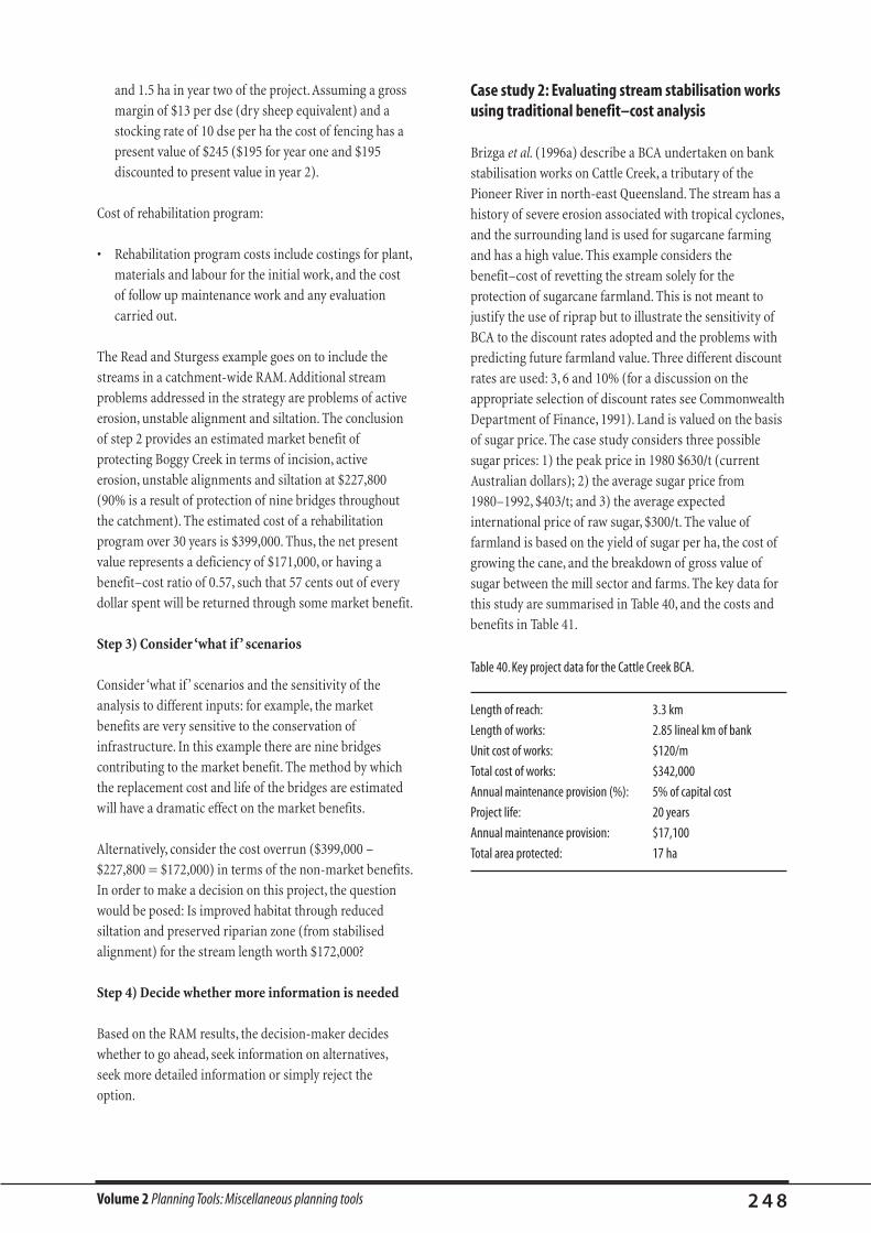
Volume 2 Planning Tools: Miscellaneous planning tools 2 4 8
and 1.5 ha in year two of the project. Assuming a gross
margin of $13 per dse (dry sheep equivalent) and a
stocking rate of 10 dse per ha the cost of fencing has a
present value of $245 ($195 for year one and $195
discounted to present value in year 2).
Cost of rehabilitation program:
• Rehabilitation program costs include costings for plant,
materials and labour for the initial work, and the cost
of follow up maintenance work and any evaluation
carried out.
The Read and Sturgess example goes on to include the
streams in a catchment-wide RAM. Additional stream
problems addressed in the strategy are problems of active
erosion, unstable alignment and siltation. The conclusion
of step 2 provides an estimated market benefit of
protecting Boggy Creek in terms of incision, active
erosion, unstable alignments and siltation at $227,800
(90% is a result of protection of nine bridges throughout
the catchment). The estimated cost of a rehabilitation
program over 30 years is $399,000. Thus, the net present
value represents a deficiency of $171,000, or having a
benefit–cost ratio of 0.57, such that 57 cents out of every
dollar spent will be returned through some market benefit.
Step 3) Consider ‘what if ’ scenarios
Consider ‘what if ’ scenarios and the sensitivity of the
analysis to different inputs: for example, the market
benefits are very sensitive to the conservation of
infrastructure. In this example there are nine bridges
contributing to the market benefit. The method by which
the replacement cost and life of the bridges are estimated
will have a dramatic effect on the market benefits.
Alternatively, consider the cost overrun ($399,000 –
$227,800 = $172,000) in terms of the non-market benefits.
In order to make a decision on this project, the question
would be posed: Is improved habitat through reduced
siltation and preserved riparian zone (from stabilised
alignment) for the stream length worth $172,000?
Step 4) Decide whether more information is needed
Based on the RAM results, the decision-maker decides
whether to go ahead, seek information on alternatives,
seek more detailed information or simply reject the
option.
Case study 2: Evaluating stream stabilisation worksusing traditional benefit–cost analysis
Brizga et al. (1996a) describe a BCA undertaken on bank
stabilisation works on Cattle Creek, a tributary of the
Pioneer River in north-east Queensland. The stream has a
history of severe erosion associated with tropical cyclones,
and the surrounding land is used for sugarcane farming
and has a high value. This example considers the
benefit–cost of revetting the stream solely for the
protection of sugarcane farmland. This is not meant to
justify the use of riprap but to illustrate the sensitivity of
BCA to the discount rates adopted and the problems with
predicting future farmland value. Three different discount
rates are used: 3, 6 and 10% (for a discussion on the
appropriate selection of discount rates see Commonwealth
Department of Finance, 1991). Land is valued on the basis
of sugar price. The case study considers three possible
sugar prices: 1) the peak price in 1980 $630/t (current
Australian dollars); 2) the average sugar price from
1980–1992, $403/t; and 3) the average expected
international price of raw sugar, $300/t. The value of
farmland is based on the yield of sugar per ha, the cost of
growing the cane, and the breakdown of gross value of
sugar between the mill sector and farms. The key data for
this study are summarised in Table 40, and the costs and
benefits in Table 41.
Table 40. Key project data for the Cattle Creek BCA.
Length of reach: 3.3 km
Length of works: 2.85 lineal km of bank
Unit cost of works: $120/m
Total cost of works: $342,000
Annual maintenance provision (%): 5% of capital cost
Project life: 20 years
Annual maintenance provision: $17,100
Total area protected: 17 ha
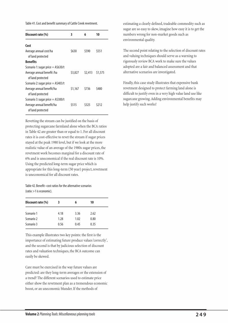
Volume 2 Planning Tools: Miscellaneous planning tools 2 4 9
Table 41. Cost and benefit summary of Cattle Creek revetment.
Discount rate (%) 3 6 10
Cost
Average annual cost/ha $630 $590 $551
of land protected
Benefits
Scenario 1: sugar price = A$630/t
Average annual benefit /ha $3,827 $2,413 $1,575
of land protected
Scenario 2: sugar price = A$403/t
Average annual benefit/ha $1,167 $736 $480
of land protected
Scenario 3: sugar price = A$300/t
Average annual benefit/ha $515 $325 $212
of land protected
Revetting the stream can be justified on the basis of
protecting sugarcane farmland alone when the BCA ratios
in Table 42 are greater than or equal to 1. For all discount
rates it is cost-effective to revet the stream if sugar prices
stayed at the peak 1980 level, but if we look at the more
realistic value of an average of the 1980s sugar prices, the
revetment work becomes marginal for a discount rate of
6% and is uneconomical if the real discount rate is 10%.
Using the predicted long-term sugar price which is
appropriate for this long-term (50 year) project, revetment
is uneconomical for all discount rates.
Table 42. Benefit–cost ratios for the alternative scenarios
(ratio >1 is economic).
Discount rate (%) 3 6 10
Scenario 1 4.18 3.36 2.62
Scenario 2 1.28 1.02 0.80
Scenario 3 0.56 0.45 0.35
This example illustrates two key points: the first is the
importance of estimating future produce values ‘correctly’,
and the second is that by judicious selection of discount
rates and valuation techniques, the BCA outcome can
easily be skewed.
Care must be exercised in the way future values are
predicted: are they long-term averages or the extension of
a trend? The different scenarios used to estimate price
either show the revetment plan as a tremendous economic
boost, or an uneconomic blunder. If the methods of
estimating a clearly defined, tradeable commodity such as
sugar are so easy to skew, imagine how easy it is to get the
numbers wrong for non-market goods such as
environmental quality.
The second point relating to the selection of discount rates
and valuing techniques should serve as a warning to
rigorously review BCA work to make sure the values
adopted are a fair and balanced assessment and that
alternative scenarios are investigated.
Finally, this case study illustrates that expensive bank
revetment designed to protect farming land alone is
difficult to justify even in a very high value land use like
sugarcane growing. Adding environmental benefits may
help justify such works!

Volume 2 Planning Tools: Miscellaneous planning tools 2 5 0
Geographic information systems (GIS) are computer-
based systems that are used to store and manipulate
geographic information such as maps. It is a simple,
relatively low-cost mapping tool that allows easy
presentation of information and is useful for managing
information. The South Australian Department of
Environment and Natural Resources set up an extensive
GIS system when developing catchment management
plans for the Inman and Torrens rivers. The following is an
assessment of the usefulness of GIS for stream
rehabilitation. As an example of cost, a ‘PC’ based GIS
system should cost around $7,000 to set up. This figure
includes software (eg. ARCVIEW/MapInfo) and a suitable
PC but it does not include any data. The cost of data is
potentially very expensive, especially if it does not exist
and needs to be ‘captured’ (ie. you have to do some field
work or spend time to crunch numbers to create the data).
The cost of data will also be expensive where it has to be
bought from government agencies or other commercial
sources. The collection and input of ‘original’ data is
expensive (in terms of collecting the data, software
requirements, and the use of highly skilled personnel) and
requires the use of the more complex and costly ARC/INFO
(as compared to ARCVIEW). However, once the data set
has been created, it is extremely cheap and easy to convert
to a PC-based GIS.
There is great potential where the data exists and can be
used on a PC GIS system (eg. ARCVIEW3). The training
time to create a competent ARCVIEW3 user is relatively
low. Bear in mind that competency in ARC/INFO is
considered to take about 3 years of full-time exposure, thus
it is an expensive system in terms of time cost in training
personnel.
THE GEOGRAPHIC INFORMATION SYSTEM(GIS) AS A STREAM REHABILITATION TOOL
By Jim Burston* and Karla Billington†
1. What is a GIS and how much does it cost to set up?
The answer to this question depends upon how you intend
to use the GIS.
Serious consideration must be given to the cost of the
information. There is a bit of an ‘industry’ pushing local
decision-makers to utilise state-of-the-art models that
require substantial quantities of data. According to Lovejoy
(1997), if the budget is limited and managers are
concerned about short-run objectives and efficiency, then
the dollars are better spent doing on-ground works rather
than data gathering. If the data are to be used for ‘one-off ’
planning decisions, then GIS is of questionable value.
However, if the data are to be distributed and widely used
by other parties, then GIS is useful. Managers should
carefully evaluate their short and long-term objectives to
determine whether low-tech or high-tech solutions are
warranted. Don’t be fooled, GIS technology does not
improve the accuracy of map data.
2. Are the analysis tools of a full-blown GIS really helpful in planning a rehabilitation project?
* South Australian Department for Environment, Heritage and Aboriginal Affairs, GPO Box 1047, Adelaide, SA 5001, Ph: (08) 8204 9108, Fax: (08) 8204 9144, Email:[email protected]†
Department of Environment and Natural Resources, Suite 2, 85 Mount Barker Rd, SA 5152. Ph: (08) 8200 3810, Fax: (08)
Volume 2 Planning Tools: Miscellaneous planning tools 2 5 1
For South Australian conditions, most of the rehabilitation
options revolve around ‘fencing and revegetation’—we
suspect that this might be the case for many other areas in
Australia. Consequently, most of the design of the
rehabilitation options is fairly crude,‘back of the envelope’
sort of stuff, where the answers are generally worked out in
the field.
A GIS has the advantage of being able to integrate different
types of spatial information (ie. land use, soils, cadastral,
stream coverage, roads etc.) and non-spatial data (eg.photos,
MS Word or Excel files).However, many of the data required
to develop an action plan for rehabilitation are either
unavailable (that’s why the Riparian Project did all the survey
work in the first place) or exist at a scale that is inappropriate.
Many of the data that are bought ‘off-the-shelf ’ require some
degree of ground-truthing to validate their accuracy.
Once the data exist, the PC-based GIS can be very useful in
developing a rehabilitation program. It can help determine
the length of watercourse affected, the cost of repairs, on
whose property the works are to be undertaken, production
of summary tables for issues/sub-catchments/local council
areas or what ever else is required. This can all be done in a
very short time. Furthermore, it has a great capacity for
monitoring and auditing (ie. what/where/when/cost) a
rehabilitation program (as we have set up for the work
being done in the River Torrens).
GIS is now widely accepted as the standard format for data
storage. The advent of PC GIS enables ease of access for all
resource managers.
The standard GIS model employs co-ordinates (ie.
latitudes and longitudes) to define segments or points
along a watercourse (the arc-node model). We have
experienced difficulties with the analysis of data,
particularly when measurements are required between
different features along a watercourse. Other problems
included inefficient storage of data (especially for
segmented linear data) and difficulties in overlaying and
analysing linear and point data.
If there is a strong requirement for analysis, then the
ARC/INFO package ‘Dynamic Segmentation’ (DS) has great
potential. To the best of our knowledge, we are the only
people using this package for stream rehabilitation work in
Australia.
DS is a system for measuring changes along a linear
network (eg. roads, sewers, electricity grid, stream
network). The strength of this package is in its ability to
analyse data that may change along a stream network (eg.
water quality). It is also useful for analysing between
various data sets (eg. location of knick points, type of bed
material, bank stability). DS enables the development of
more complex and flexible models. Its real value may be
best exploited by those who want to understand the
underlying processes and mechanisms of stream
processes and the water quality of those streams.
If you just want to ‘fix up’ the river, then don’t worry about
Dynamic Segmentation.
3. Analysis of GIS information
The integration of spatial and non-spatial information
makes this an extremely valuable resource for managers. It
enables users to view the current condition of the
watercourse and then use the ARCVIEW format as a tool
for monitoring, auditing and displaying the results
achieved in implementing on-ground works. Furthermore,
all this information can be written to a CD-ROM, with
accompanying documentation, to greatly increase the
accessibility of the data.
If you’re going to use GIS, you must ensure that at least one
member of the project team is a GIS expert, who can
‘trouble-shoot’ as required and train other staff.
4. Data transfer

Volume 2 Planning Tools: Miscellaneous planning tools 2 5 2
For whole of catchment rehabilitation project – YES.
For the treatment of isolated reaches of watercourse –
generally NO.
Benefits: ease of access to data; monitoring/costing of
rehabilitation options; GIS is recognised as a standard
data storage format; there is a lot of undeveloped potential
in the ARC/INFO package,‘Dynamic Segmentation’, for the
analysis of river processes.
5. Is the effort and cost of GIS worth it? What arethe benefits and costs?

Volume 2 Planning Tools: Miscellaneous planning tools 2 5 3
SOME COSTS OF STREAM REHABILITATIONACTIVITIES
Please note that this manual does not provide detailed
financial advice and the following tables are a general guide
only.
It is useful for stream rehabilitators to have an idea of the
potential cost of rehabilitation works. The following tables
and notes are the beginnings of what we hope will be a
more comprehensive inventory of the costs of
rehabilitating streams in Australia. Most of the following
data were taken from White et al. (1999), whose paper also
includes other interesting statistics on the money being
spent on stream rehabilitation in Australia at present. Note
that the DLWC River Management Unit (NSW) has
published excellent tables for estimating the cost of works
in streams (published in 1994).
All values are in 1997–98 Australian dollars. These values
can be corrected in the future for inflation by using the
consumer price index.
Traditional stream management of degraded streams
(including stabilisation of the bed and banks) can be very
expensive (often in the order of tens to hundreds of
thousands of dollars per stream kilometre), but rehabilitation
of degraded streams is likely to cost even more. In part, this is
because of the extra assessment and evaluation costs that are
often associated with rehabilitation work.
Indicative unit rates for some stream rehabilitation
projects, techniques and resources are provided in Tables
43 and 44. It should be noted that the rates will be highly
variable and will depend on factors including: the size of
the stream, establishment costs for equipment at a site,
distance from work centres to work sites, and climatic and
other environmental conditions.
1. The costs of stream management works
Table 43.The scale of stream rehabilitation project costs.
Item Indicative unit rate Source
Full revegetation (from tube-stock), and fencing, of a riparian strip on both banks of a $12,000 per km R. Hardie, pers. comm.
stream (direct seeding of vegetation may be considerably cheaper).
Typical rock chute in a small creek (say streams up to 15 m wide, 1 m drop, $5,000–$20,000 per chute R. Hardie, pers. comm.
length 10 m, apron length 4 m, plus abutment protection).
Fishways:
• rock ramp (up to 2 m vertical) $10,000–$30,000 per vertical metre T. O’Brien, pers. comm.
• vertical slot (3–6 m vertical) $60,000–$100,000 per vertical metre
(Total cost of 1 m rock ramp fishway
= $10,000, using 24 m3 of rock).

Volume 2 Planning Tools: Miscellaneous planning tools 2 5 4
Item Indicative unit rate Source
Stabilisation and revegetation of degraded urban streams (eg. Melbourne streams). $0.5–$0.8 million per kilometre Melbourne Water
($500–$800 per linear metre)
Flow alignment works (eg. retards). $20,000–$50,000 per bend on R. Hardie pers. comm.
medium-sized rivers John Gardiner, DLWC, NSW
Using ‘Jacks’ on a NSW stream
= $10,000 for a single bend
Twentymile Creek, Mississippi, USA. Stream rehabilitation involving grade control, $0.5 million per km (Danley et al., 1995)
alignment training, revegetation of an incised stream.
Table 44. Costs of stream rehabilitation resources (most values come from ID&A Pty Ltd).
Item Indicative unit rate
Seed from native species (commercial collection) . $170/kg (Burston and Brown, 1996)
Tree seedlings:
• 10 cm to 20 cm $0.50 to $1.00 each
• seedlings (which are small) $0.20 to $0.40 each
Tree planting (including preparation, planting, excluding maintenance) $3.00/tree
Willow control—lopping (including safeguards to stop willow spread)
followed up by herbicide treatment:
• Moderate infestation $3,500/km of bank
• Severe infestation $6,000/km of bank
• Intensive infestation $12,000/km of bank
Fencing materials $2.50 per metre of fence
Excavator hire:
• 12 tonne $65 per hour
• 20 tonne $85 to $100 per hour
• 30 tonne $100 to $130 per hour
Broken rock (delivered) $15 to $25 per cubic metre delivered
($9.40–$15.60 per tonne)
Railway line (which can be used as piles) $20 per metre
Timber that can be used in rails of flow retards:
• Red box, 150 to 300 mm diameter, 4 m length $10–$15 each
• Red box, 150 to 300 mm diameter, 6 m length $12 to $20 each
Labour:
• Project works supervisor $15–$25/hour
• Works crew member $15/hour
Survey team (surveyor, assistant, basic equipment) $100/hour
Engineering design and supervision 10–15% of project cost
Administration 5–10% of project cost
Table 43 (cont’d).The scale of stream rehabilitation project costs.
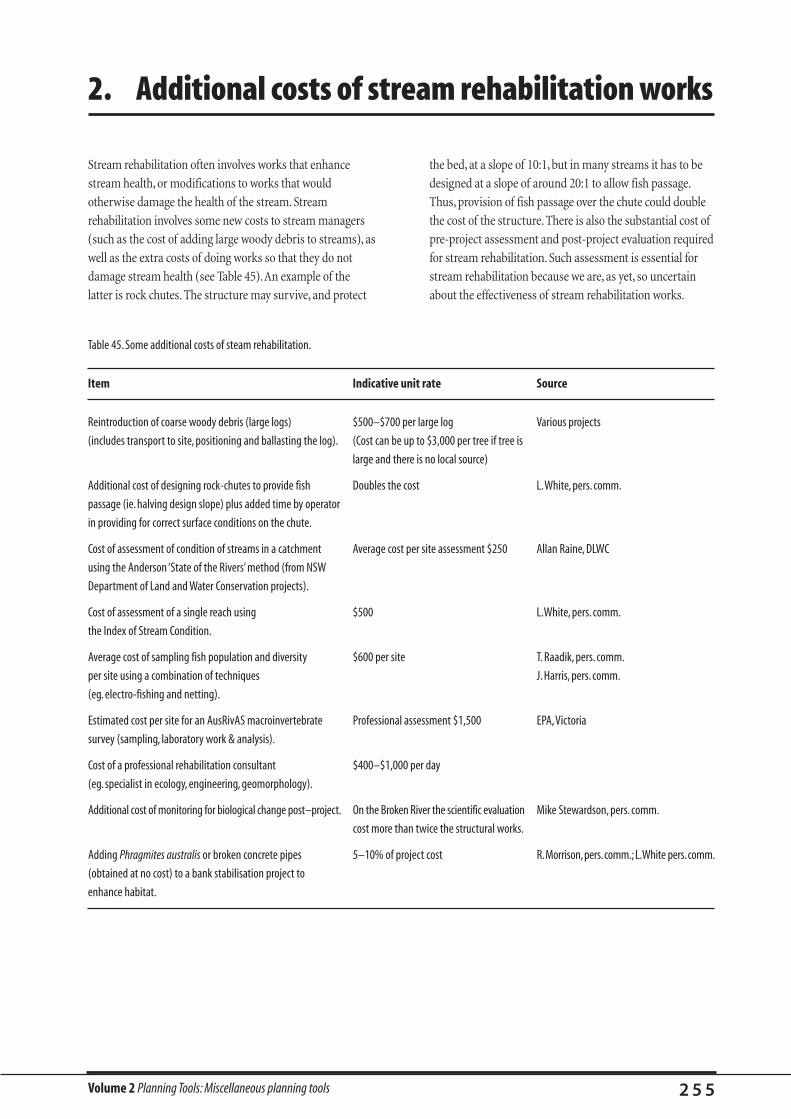
Volume 2 Planning Tools: Miscellaneous planning tools 2 5 5
Stream rehabilitation often involves works that enhance
stream health, or modifications to works that would
otherwise damage the health of the stream. Stream
rehabilitation involves some new costs to stream managers
(such as the cost of adding large woody debris to streams), as
well as the extra costs of doing works so that they do not
damage stream health (see Table 45).An example of the
latter is rock chutes. The structure may survive, and protect
the bed, at a slope of 10:1, but in many streams it has to be
designed at a slope of around 20:1 to allow fish passage.
Thus, provision of fish passage over the chute could double
the cost of the structure. There is also the substantial cost of
pre-project assessment and post-project evaluation required
for stream rehabilitation. Such assessment is essential for
stream rehabilitation because we are, as yet, so uncertain
about the effectiveness of stream rehabilitation works.
2. Additional costs of stream rehabilitation works
Table 45. Some additional costs of steam rehabilitation.
Item Indicative unit rate Source
Reintroduction of coarse woody debris (large logs) $500–$700 per large log Various projects
(includes transport to site, positioning and ballasting the log). (Cost can be up to $3,000 per tree if tree is
large and there is no local source)
Additional cost of designing rock-chutes to provide fish Doubles the cost L.White, pers. comm.
passage (ie. halving design slope) plus added time by operator
in providing for correct surface conditions on the chute.
Cost of assessment of condition of streams in a catchment Average cost per site assessment $250 Allan Raine, DLWC
using the Anderson ‘State of the Rivers’ method (from NSW
Department of Land and Water Conservation projects).
Cost of assessment of a single reach using $500 L.White, pers. comm.
the Index of Stream Condition.
Average cost of sampling fish population and diversity $600 per site T. Raadik, pers. comm.
per site using a combination of techniques J. Harris, pers. comm.
(eg. electro-fishing and netting).
Estimated cost per site for an AusRivAS macroinvertebrate Professional assessment $1,500 EPA,Victoria
survey (sampling, laboratory work & analysis).
Cost of a professional rehabilitation consultant $400–$1,000 per day
(eg. specialist in ecology, engineering, geomorphology).
Additional cost of monitoring for biological change post–project. On the Broken River the scientific evaluation Mike Stewardson, pers. comm.
cost more than twice the structural works.
Adding Phragmites australis or broken concrete pipes 5–10% of project cost R.Morrison,pers.comm.; L.White pers.comm.
(obtained at no cost) to a bank stabilisation project to
enhance habitat.

Volume 2 Planning Tools: Miscellaneous planning tools 2 5 6
A great deal of valuable information on stream
rehabilitation exists in the form of fact sheets. These
information sheets are produced mostly by government
departments and community groups, and often consist of
information in a form that is simple, clear and easy to use.
Most of these sheets are produced at a State or even
catchment level. This means that, although the
information is often more widely applicable, the
community groups and stream managers outside the
region where the fact sheet was produced are unlikely to
know of its existence. In this section we present a list of
the fact sheets that we are aware of, as well as the contact
details of the organisations that distribute them. In this
way, we hope to encourage communication within the
Australian stream management community.
BIBLIOGRAPHY OF SOME TECHNICALINFORMATION AVAILABLE IN AUSTRALIA
The fact sheets below are arranged by broad subject, and,
where relevant, the specific subjects are listed in italics after
the entry. Table 46 explains the abbreviations and provides
addresses of organisations that produce the sheets.
1.1. Assessment of stream condition
Anderson, J. (1993). State of the rivers: Maroochy River
and tributary streams. Maroochy, Qld, Maroochy
Shire Council & Department of Primary Industries.
(State of environment reporting, bank erosion, riparian
vegetation, assessment, Aust. aquatic habitat,
conservation, riparian vegetation, bed, bank, bar, overall
condition rating, Coolum Creek, Doonan Creek, Yaninda
Creek, Petrie Creek, Browns Creek, York Creek, Eudli
Creek)
AVRMA (1994). River management works—the
picture after the ’93 floods, Association of Victorian
River Management Authorities.
(Broken river, Ovens river, Victoria, brushing, riprap,
riffle, rock weir)
Brierley, G. J., K. Fryirs and T. Cohen (1996).
Geomorphology and river ecology in southeastern
Australia: An approach to catchment
characterisation: Part one: a geomorphic approach
to catchment characterisation. Sydney, Australia,
Graduate School of the Environment, Macquarie
University.
(geomorphology, descriptors, Australia, river structure,
stream classification, restoration, rehabilitation,
hierarchical, procedure, prediction)
DNRE (1997). Index of stream condition: Trial
applications, Department of Natural Resources and
Environment (Vic).
(Victoria, stream conservation, stream measurements,
stream ecology, water quality, Gippsland)
DNRE (1997). Index of stream condition: A reference
manual, Department of Natural Resources and
Environment (Vic).
(Victoria, stream conservation, stream measurements,
stream ecology, water quality, Latrobe catchment, Broken
River)
DNRE (1997). Index of stream condition: Users
manual, Department of Natural Resources and
Environment (Vic).
(Victoria, stream conservation, stream measurements,
stream ecology, water quality, planning, data collection)
QDPI (1993). The condition of river catchments in
Queensland, Queensland Department of Primary
Industries.
(Queensland, rivers, catchment management, erosion,
flooding, salinity, chemicals, water quality, weeds, urban
expansion, channel instability, habitat loss, vegetation,
wetlands, fish, fauna, ecology)
1. A bibliography of fact sheets

Volume 2 Planning Tools: Miscellaneous planning tools 2 5 7
Waterwatch Victoria (1995). A waterwatch guide to
conducting habitat surveys. DNRE (VIC).
(evaluation, monitoring)
1.2. Stream stability
Carter, J. and E. Cottingham. A guide to erosion control
measures for small watercourses in the Mount
Lofty Ranges, Water Resources Group, Department of
Environment and Natural Resources, SA.
(bed erosion control, bank erosion control, terminology
and definitions, watercourse management, problem
assessment, strategies, soil stabilisation, riparian
vegetation, techniques, slides)
DWR. River wrongs: over removal of gravel, New South
Wales Department of Water Resources.
(gravel removal, channel straightening, excavation,
cut-off, New South Wales)
DWR. The 7-Step method of controlling bank erosion
and sediment build-up Plus: Prevention methods
you can use now, New South Wales Department of
Water Resources. (maintenance, expert advice,
sedimentation, permission, funding, advice, New South
Wales)
Hader, W. and D. Outhet (1995). Works to control stream
bed erosion. Treatment option: Boulders, DLWC.
(Schauberger weirs, bed stabilisation, artificial riffle)
Hader, W. and D. Outhet (1995). Works to control stream
bed erosion. Treatment option: Log/timber v weir
(horizontal or vertical logs), DLWC.
(Schauberger log sill, bed erosion, riffle, pool, scour)
LWRRDC. (1996). Streambank stability. Riparian
management.
(bank erosion, riparian vegetation, stabilisation, plant
species, revegetation)
Outhet, D. (1995). Extractive industries on floodplains.
Best management practices. DLWC.
(sand extraction, gravel extraction, mining, NSW)
Outhet, D. (1995). Extractive industries on river bars.
Best management practices. DLWC.
(sand extraction, gravel extraction, bed degradation, flow
diversity, river turbidity)
Outhet, D. (1995). Works to control stream bed erosion.
Treatment option: log and rock bed control and
road crossing (gravel/sand/silt road surface) on
small intermittent flow stream, DLWC.
(headcut, ford, vehicle crossing)
DLWC Riverine Management Unit (1994). Works to
control stream bank erosion. Treatment option:
Brush groynes and vegetation.
(bank stabilisation)
DLWC Riverine Management Unit (1994). Works to
control stream bank erosion. Treatment option:
Gravel mesh sausages and vegetation.
(bank stabilisation)
DLWC Riverine management unit (1994). Works to
control stream bank erosion. Treatment option:
Heavy duty mesh fencing and vegetation.
(retards, bank stabilisation)
DLWC Riverine Management Unit (1994). Works to
control stream bank erosion. Treatment option:
Jacks and vegetation.
(bank stabilisation, jacks)
DLWC Riverine Management Unit (1994). Works to
control stream bank erosion. Treatment option: log
wall and vegetation.
(toe protection)
DLWC Riverine Management Unit (1994). Works to
control stream bank erosion. Treatment option:
Rock revetment and vegetation.
(riprap, revegetation)
DLWC Riverine Management Unit (1994). Works to
control stream bank erosion. Treatment option:
Timber groynes and vegetation.
(bank stabilisation, groynes)
DLWC Riverine Management Unit (1994). Works to
control stream bank erosion. Treatment option:
Rock groynes and vegetation.
(bank stabilisation)
West, S. and D. Outhet (1995). Restoring urban streams.
Treatment option: reconstructing vegetated
meander bends in straightened channels,
DLWC, NSW.
(channelisation, channelisation, pool, riffle, meander)
Volume 2 Planning Tools: Miscellaneous planning tools 2 5 8
1.3. Vegetation
Anon. (1995). Hand direct seeding of native plants,
Primary Industries, SA.
(native vegetation, revegetation, weed control, sowing,
native trees, South Australia)
Ardill, S. (1994). Wetlands on your farm, DLWC, NSW.
(wetland restoration, wetland rehabilitation, definition)
Carter, J. (1993). WATERWISE—exotic trees along
watercourses, Water Resources Group, Department of
Environmental and Natural Resources.
(siltation, willows, ash, poplar, weed control)
Carter, J. (1993). WATERWISE—woody weed control
along watercourses, Water Resources Group,
Department of Environment and Natural Resources.
(gorse, blackberry)
Cremer, K., C.Van Kraayenoord, N.Parker and
S.Streatfield(1995). Willows spreeding by seed,
Australian Journal of Soil and Water Conservation 8
(4): 18–27.
(exotic, weed)
DENR (1993). WATERWISE: Revegetation of
watercourses, Water Resources Group, Department of
Environment and Resources (SA).
(bank stability, buffering)
LWRRDC (1996). Land-based ecosystems, Riparian
management fact sheet.
(riparian vegetation, ecology)
LWRRDC (1996). River ecosystems, Riparian
management fact sheet.
(riparian vegetation)
LWRRDC (1998). Managing snags in rivers, Riparian
management fact sheet.
(fact sheet, LWD, desnagging, resnagging)
QDNR. Control of azolla: red water fern.
QDNR. Control of cumbungi.
QDNR. Control of exotic vines.
QDNR. Control of salvinia.
QDNR. Control of water hyacinth: the worst aquatic
weed in the world.
QDNR .Growing trees in frost-prone areas.
QDNR. Planting trees in dry areas or with limited
water.
QDNR. Plants suitable for salty soils.
QDNR. Plants suitable for sandstone or shale areas.
QDNR. Plants suitable for western Qld.
QDNR. Propagation of trees and shrubs from seed.
QDNR. Seed collection, storage and testing.
QDNR. Tree retention.
QDNR. Water requirements for trees.
QDNR. Weed control for tree planting.
Raine, A. and J. Gardiner, 1997a. Revegetating streams in
the Clarence Catchment. A guide to species and
planting methods, New South Wales Government.
(riparian vegetation, revegetation, suitable species, bank
stabilisation)
Raine, A. and J. Gardiner, 1997b. Revegetating streams in
the Macleay Catchment. A guide to species and
planting methods, New South Wales Government.
(riparian vegetation, revegetation, suitable species, bank
stabilisation)
Raine, A. and J. Gardiner, 1997c. Revegetating streams in
the Manning Catchment. A guide to species and
planting methods, New South Wales Government.
(riparian vegetation, revegetation, suitable species, bank
stabilisation)
Raine, A. and J. Gardiner (1997). Revegetating streams in
the Bellinger Catchment. A guide to species and
planting methods, New South Wales Government,
DLWC.
(riparian vegetation, revegetation, suitable species, bank
stabilisation)
Volume 2 Planning Tools: Miscellaneous planning tools 2 5 9
Raine, A., J. Golding, et al. (1997). Revegetating streams
in the Brunswick Catchment. A guide to species
and planting methods, New South Wales
Government, DLWC.
(riparian vegetation, revegetation, suitable species, bank
stabilisation)
Raine, A., T. Hudson, et al. (1997). Revegetating streams
in the Nambucca Catchment. A guide to species
and planting methods, New South Wales
Government, DLWC.
(riparian vegetation, revegetation, suitable species, bank
stabilisation)
DLWC Riverine Management Unit (1994). Controlling
willows.
(willow eradication, drill and fill, poison)
Roberts, K. (1992). Buffer zones along rivers and
creeks, DWR.
(water quality, riparian vegetation, buffer strips)
S.A. Department of Environment and Natural Resources.
Exotic trees along watercourses.
S.A. Department of Environment and Natural Resources.
Revegetating watercourses.
1.4. Animals
Anon. Electric fencing for sheep and cattle in the hills,
Tungkillo and Harrogate Landcare Groups.
(stock exclusion)
Anon. (1997). Ripples. Newsletter of the Australian
Platypus Conservancy, Philips and Father.
(platypus, stream health, ecology, community, habitat
improvement)
Nicholas, S. and Mack, P. (1996). Manage your banks: A
practical guide to stream-side management,
fencing and water supplies, The Goulburn Valley
Environment Group.
(protection of stream banks, fencing, watering systems,
stock management, weed control, vermin control, fire
hazard control, flood gates, creek crossing, water
distribution, restricted access, water diversions, dams,
groundwater, pumping, offstream watering, Australia)
QDNR. Trees attractive to birds.
1.5. Water quality and pollution
Anon. (1994). Disposal of farm chemical containers,
DWR (NSW).
(pollution, contamination, water quality)
Anon. (1994). Filter zones for farm dams, DWR (NSW).
(buffer strip, water quality, silt trap)
Anon. (1994). Small farms and septic tanks, DWR
(NSW).
(nutrient, water quality)
Bek, P. (1992). Blue-green algae in farm dams, DWR
(NSW).
(water quality, nutrient, toxic blooms)
Carter, J. (1993). WATERWISE—farm dams for stock,
wildlife and improved water quality, Water
Resources Group, Department of Environmental and
Natural Resources (SA).
(features, intake, filters, fencing, vegetation silt traps,
islands)
LWRRDC (1996). Water quality. Riparian management.
(riparian vegetation, buffer strips)
QDNR. Water requirements: stock and domestic
purposes.
Smith, M., W. Kay, et al. (1997). Spineless indicators,
Department of Conservation and Land Management
(WA).
(macroinvertebrate, monitoring, Western Australia)
LWRRDC (1996). Water quality. Riparian management fact
sheet. (riparian vegetation, buffer strips)
1.6. Environmental flows
Anon (1995). Water allocation & management
planning, DPI, Queensland.
(ecologically sustainable development, management,
water entitlements, Queensland)
Cullen, P. (1994). A rationale for environmental flows.
AWWA Environmental Flows Seminar.
(water entitlements, water quality, river channels,
floodplain areas, river regulation, aquatic life,
maintenance flows, major floods)

Volume 2 Planning Tools: Miscellaneous planning tools 2 6 0
1.7. Management of rivers: procedures andexamples
Burston, J., and Good, M. (1995). Watercourse
management guidelines for the Inman River
catchment, Adelaide, Department of Environment and
Natural Resources, Adelaide, South Australia.
(riparian zone, stream order, channel change, gravel
extraction, urbanisation, erosion, management issues,
rehabilitation, community participation, point source
pollution, water quality)
Burston, J., Aucote, M., Eaton, A. and Prider, A. (1997).
Torrens 1997—an action plan for better
watercourse management, Adelaide, Department of
Environment and Natural Resources, Adelaide, South
Australia.
(riparian zone, stream order, channel change, erosion,
management issues, rehabilitation, community
participation, revegetation, bird life, weed removal,
stabilising structures, fencing, native flora, soils in
research area, macroinvertebrates)
Carter, J. (1993). WATERWISE—watercourse
management, Water Resources Group, Department of
Environmental and Natural Resources.
(erosion, water quality, wildlife, property value, stream
processes, riparian zone, native vegetation, willows,
buffer zones, revegetation, total catchment management)
DWR. A guide to stream channel management, New
South Wales Department of Water Resources.
(clearing, excavating, diverting, management, infilling)
Victorian Department of Conservation and Environment
(1990). Environmental guidelines for river
management works,Vic DCE.
(morphology, ecology, rock beaching, brushing, groynes,
alignment training, snag management, revegetation,
sand and gravel extraction, rock chutes, drop structures,
channel modification, bank battering, meander cutoffs,
lopping, levee banks, LWD, channelisation)
Myers, R., Ed. (1993). Watercourse management: A field
guide. Upper River Torrens Landcare Group (SA).
(Upper Torrens Valley history, revegetation of
watercourses, bird life, stabilisation of watercourses,
management of watercourses, weed removal, stabilising
structures, fencing, native grasses, soils in research area,
pasture establishment, frogs, macroinvertebrates)
NSW DWR. A guide to stream channel management:
clearing, diverting, excavating, infilling, New South
Wales Department of Water Resources.
(clearing, excavating, diverting, management, infilling,
legal requirements, regulatory bodies, permits, New South
Wales)
Queensland DPI (1993). A guide to integrated
catchment management in Queensland, ICM and
Landcare Unit, Brisbane.
(rivers of Queensland, treecare, Mary river, Murray
Darling Basin, Johnstone River, Lockyer Valley, Pioneer
River, Mitchell River, catchments)
Raine, A.W. and J.N. Gardiner (1995). Rivercare:
guidelines for ecologically sustainable
management of rivers and riparian vegetation,
LWRRDC.
(rehabilitation, restoration, NSW, revegetation)
RCMU (1993). River management: why bother?
Riverine Corridor Management Unit, Department of
Water Resources (DWR) (NSW).
(New South Wales, River Management Program,
community)
Working Group on Waterway Management (1992).
Guidelines for stabilising waterways, Melbourne,
Standing Committee on Rivers and Catchments,
Victoria.
(river management, design guidelines, problem
assessment, drop structures, drainage, waterway outlets,
low flow pipelines, floodways, retarding basins, rock
riprap, rock chutes, retards, groynes)
1.8. Policy guidelines and legal considerations
DPI. The sustainable use and management of
Queensland’s natural resources: polices and
strategies.
(discussion of approach to developing long term planning
for Qld’s natural resources)
Parlavliet, G. J. (1993). Proceedings of the Blackwood
Catchment Drainage Workshop, Blackwood
Catchment Drainage Workshop, Bridgetown, November
1993, Blackwood Catchment Coordinating Group.
(community management, government planning,
community consultation, WA)

Volume 2 Planning Tools: Miscellaneous planning tools 2 6 1
Parlavliet, G. J. (1993). Proceedings of the Blackwood
Catchment Drainage Workshop, Blackwood
Catchment Drainage Workshop, Katanning, September
1993, Blackwood Catchment Coordinating Group.
(community influence, government policy, WA)
Parlevliet, G. J. (1994). Proceedings of the Blackwood
Catchment Drainage Workshop, Blackwood
Catchment Drainage Workshop, Kojonup, April 1994,
Blackwood Catchment Coordinating Group.
(remnant vegetation, protection, policy, economic value,
community consultation, government, WA)
WRC (1993). The NSW State Rivers and Estuaries
Policy, NSW Water Resources Council, New South
Wales Government.
(New South Wales)
1.9. General information about rivers
CRCFE (1996). The Murray–Darling Freshwater
Research Centre's Lower Basin Laboratory.
Working together for the future of freshwater
resources, Cooperative Research Centre for Freshwater
Ecology, The Murray–Darling Freshwater Research
Centre.
(floodplains, billabongs, floods, ecology, algae,
Barwon–Darling River, Murray River, carp)
Department of Land and Water Conservation (1996).
Rivercare 2000—Achievements Year Book 1995.
(wetland rehabilitation, urban run-off treatment,
salinity, realignment)
Department of Land and Water Conservation (1996).
Rivercare 2000 Special Edition—CURRENTS.
(stream rehabilitation, New South Wales, community
awards)
Department of Land and Water Conservation (1995).
Managing the water resources of New South Wales:
A survey of landholder and community attitudes,
Sydney.
(landholder survey, sustainable riverine management,
community perception)
Myres, R. (1993). Watercourse management. A field
guide, Landcare South Australia. Upper River Torrens
Landcare Group.
(weed removal, stream bed stabilisation, bank
stabilisation, native plant revegetation, pasture
establishment, Mount Lofty Ranges, macro invertebrates,
fencing, woody weeds, native grasses, birds, direct
seeding)

Volume 2 Planning Tools: Miscellaneous planning tools 2 6 2
Table 46. A list of abbreviations and contact details.
Abbreviation Name Address
Association of Victorian River Management Authorities (VIC) See DNRE (VIC)
AWWA Australian Wastewater and Water Association PO Box 388 Artarmon NSW 1570
Ph (02) 9413 1288
Catchment Resource Centre Mount Lofty Ranges Catchment Group
5c Cameron St Mount Barker
SA 5251
DEHAA Department for Environment, Heritage and Aboriginal GPO Box 1047 Adelaide
Affairs (South Australia) SA 5001
DC&E (VIC) Department of Conservation and Environment (Vic)
— see DNRE (Vic)
CALM (WA) Department of Conservation and Land Management General Switch
(Western Australia) Ph 08 9334 0333
DENR (SA) Department of Environment and Natural Resources
(South Australia)— see DEHAA
DENR Department of Environment and Natural Resources (VIC)
— see DNRE
DLWC Department of Land and Water Conservation 10 Valentine Ave PO Box 3720
Parramatta NSW 2150
Ph +61 (02) 9895 6211
Fax: +61 (02) 9895 7281
QDNR Department of Natural Resources (QLD) General Enquiries
Ph (07) 3896 3111
DNRE Department of Natural Resources and Environment (VIC) PO Box 500 East Melbourne Vic
Ph (03) 9412 4011
DPI (Tas) Department of Primary Industries (Tas) — see DPIWE
DPIF (Tas) Department of Primary Industries and Fisheries (TAS)
— see DPIWE
2. Abbreviations and contact details

Volume 2 Planning Tools: Miscellaneous planning tools 2 6 3
Abbreviation Name Address
DPIWE Department of Primary Industries,Water and Environment (TAS) GPO Box 44A Hobart Tasmania
Ph (03) 6233 6496
DWR Department of Water Resources, NSW— see DLWC
GVEG Goulburn Valley Environment Group (Vic)
LWRRDC Land and Water Resources Research and Development Corporation Level 2, UNISYS Building
91 Northbourne Ave Turner
Canberra 2612
Ph (02) 6257 3379
www.rivers.gov.au
Melbourne Standing Committee on Rivers and Catchments
— see DNRE (Vic)
Primary Industries of South Australia — see DEHAA
QDPI Queensland Department of Primary Industries General Enquiries
Ph (07) 3239 3111
Ripples Ripples Newsletter of the Australian Platypus Conservancy PO Box 84 Whittlesea VIC 3757
Upper River Torrens Landcare Group PO Box 250 Birdwood SA 5234
Ph (08) 8568 5339
Water Resources Commission
— see DLWC (NSW)
Table 46 (cont’d). A list of abbreviations and contact details.

PART 3:INTERVENTION
TOOLS
formation. A general rule is that the stream bed must be
stabilised before the stream banks are considered. Hence,
for many incising streams, full-width structures are the
starting point for stream rehabilitation. Full-width
structures covered in this manual are low weirs, including
log sills, rock and gabion dams, artificial riffles, and rock
chutes. Special attention is paid to the ability of fish to
negotiate full-width structures. Fishway design techniques
for modifying full-width structures so that they are not a
barrier to fish passage are described.
2. Partial-width instream structures
Partial-width instream structures are commonly adopted
to stabilise eroding banks. Partial-width structures can be
either impermeable, eg. groynes or low deflectors, or
permeable, eg. retards. Which particular type of partial-
width structure is applied depends on stream conditions,
available material and the desired result. Depending on the
structure used, partial-width structures can:
• protect the banks;
• create deposition zones;
• realign the channel;
Most attempts at improving in-stream habitat are based
first on providing a stable channel, and second on
providing increased hydraulic diversity. Examples of
increased hydraulic diversity include the creation of deep,
slow sections of the channel with scour pools, and higher
velocity riffle areas. Shields (1984) argues that the most
effective habitat structures create a diversity of velocities,
depths, substrates, and illumination conditions that mimic
the natural stream. Note that the rehabilitation benefits of
many in-stream structures come from the reduced
erosion, altered flow hydraulics, and local scour. The local
scour around structures is discussed in Predicting the
scour produced when you put things into streams, in Natural
channel design, this Volume.
Note that there are some fundamental concepts under-
pinning the use of in-stream structures. These principles
are discussed in Step 9. What is the detailed design of your
project in the Stream rehabilitation procedure,Volume 1.
This chapter has ten sections:
1. Full-width instream structures
Full-width instream structures are used primarily to stop
bed degradation and to enhance in-stream habitat by pool
Volume 2 Intervention Tools 2 6 5
This chapter describes some of the structural tools
available for rehabilitating streams. It is broken into two
sections, Intervention in the channel, and Intervention in
the riparian zone.
1. Intervention in the channel
INTRODUCTION TO THE INTERVENTIONTOOLS SECTION
Note that this is not a structural design manual. Detailed
design procedures for many of the structures described here
are provided in texts elsewhere, such as the ’Guidelines for
Stabilising Waterways‘ (Working Group on Waterway
Management, 1991). In this section we will emphasise the
environmental role of each design.Where a technique is new,
and has not been described elsewhere, we may include some
general design information. Please note that very useful
information on a range of interventions is provided in the New
South Wales Department of Land and Water Conservation’s
‘Riverwise’ guidelines for stream management.

Volume 2 Intervention Tools 2 6 6
• train the channel to a new course;
• narrow an overwide channel; and/or
• create low-velocity zones suitable for the establishment
of vegetation.
3. Longitudinal bank protection techniques
The most direct way to treat unacceptable rates of bank
erosion is through direct armouring of the bank surface.
This section provides details of environmentally friendly
methods of protecting the toe of the bank and the bank
face, including longitudinal stone toe protection, brushing,
beaching, rock revetment, and hybrid techniques.
4. Bed replenishment
5. Reinstating meanders that have been artificially cut off
6. Fish cover
7. Boulders
8. Overcoming barriers to fish passage
9. Management of large woody debris
10.Sand and gravel extraction as a rehabilitation tool
Commercial sediment extraction from non-tidal streams
usually leads to environmental damage. Nevertheless,
there are a few situations in which extraction can be a
useful tool for stream rehabilitation, particularly in
managing sediment slugs.
The stream ecosystem does not stop at the water’s edge,
but includes the riparian zone and floodplain habitat.
Riparian vegetation is dependent on the stream for water
supply, and is often influenced by the flooding regime. The
vegetation also plays a major role in the in-stream ecology,
providing food (leaf litter and insects), and habitat (snags)
the stream, and influencing bank stability and water
quality. Intervention in the riparian zone comes in the
form of managing the plant species present, and managing
stock access. This chapter has four sections.
1. Vegetation management
This section discusses how vegetation acts to stabilise
stream banks, and therefore what you should plant where,
to get the best effect on bank stability. It also describes the
methods available for establishing riparian vegetation.
2. Streams infested by exotic weeds
This section briefly describes the problems exotic (ie. not
locally native) weed species can cause in the riparian zone,
and lists some fact sheets available from government
departments which provide advice on the control of many
common weeds.
3. Willow-infested streams
Willows are only one of many types of exotic vegetation,
but so much effort is put into their control in south-
eastern Australia that they have their own section
outlining the effects they have on streams, and the
methods that have been developed to control them.
4. Managing stock access to streams
This section outlines the pros and cons of the different
types of fencing that are suitable for excluding stock from
the stream, and the options available for off-stream
watering of stock.
2. Intervention in the riparian zone

INTERVENTION IN THE CHANNEL
• Full-width structures
• Partial-width bank erosion control structures
• Longitudinal bank protection
• Bed replenishment
• Reinstating cut-off meanders
• Fish cover
• Boulders
• Overcoming barriers to fish passage
• Management of large woody debris
• Sand and gravel extraction as a rehabilitationtool

Volume 2 Intervention Tools: Intervention in the channel 2 6 8
Full-width structures are low structures that span the full
width of the channel and are overtopped by water under
most flow conditions. They provide a backwater pool
upstream of the structure and lead to scour pool and bar
formation immediately downstream. Full-width structures
are also referred to as grade control structures, low weirs,
plunges or sills.
Full-width structures are the most common tool used to
stabilise stream beds. By acting as a hard point in the bed,
full-width structures stop the upstream migration of
headcuts. All full-width structures can be applied as a hard
point, but some are more susceptible to undermining by
the upstream migration of headcuts, as found in actively
incising streams.
The rest of this chapter and the next two chapters are split
into two groups: the first contains techniques that are
more or less proven and are commonly used due to their
wide spread suitability (although this does not mean they
will work on every stream). The second section contains
techniques that are proving popular, but must still be
considered experimental.
FULL-WIDTH STRUCTURES
The most successful full-width structures tend to be those
that can tolerate high shear-stress conditions. Thus, rock
structures tend to be the most commonly used. The ‘rock
chutes’ chapter in the Guidelines for stabilising waterways
(Working Group on Waterway Management, 1991)
provides detailed guidelines on the construction of rock
full-width structures so they will not be repeated here.
Rather, the following details are some environmental
considerations you should apply to get the best ecological
value from rock, full-width structures. These issues can
equally be applied to most of the full-width structures in
the ‘experimental full-width structures’ section.
When considering a full-width structure as part of your
stream rehabilitation strategy, take note of the following
siting constraints.
Full-width structures should be used in straight sections
of the channel (at the inflection points between bends)
(Wesche, 1985). On curved sections of the channel, the
high-flow depth and velocity are greater at the outside of
the bend, and the flow over a full-width structure is faster
than normal because of the reduced cross-sectional area.
In this situation, scour on the outside of the bend will be
greater than normal, and as a result the structure is likely
to be outflanked.
Full-width structures should be keyed into stable bank
material for 1–2 m, or 1/3 channel width, on both sides of
the channel (Wesche, 1985). A well-defined bank profile
with established vegetation is usually evidence of stable
bank material. A gravel bar that looks solid may
nevertheless be mobilised with the next large flood. The
construction of full-width structures usually requires bank
stabilisation, such as rock riprap up and downstream of
the structure to avoid outflanking.
A conservative approach to protect against downstream
scalloping due to eddy scour is to armour the channel
bank with rock for approximately 1–3 channel widths
2. Design considerations for full-width structures
1. Tried and true full-width structures
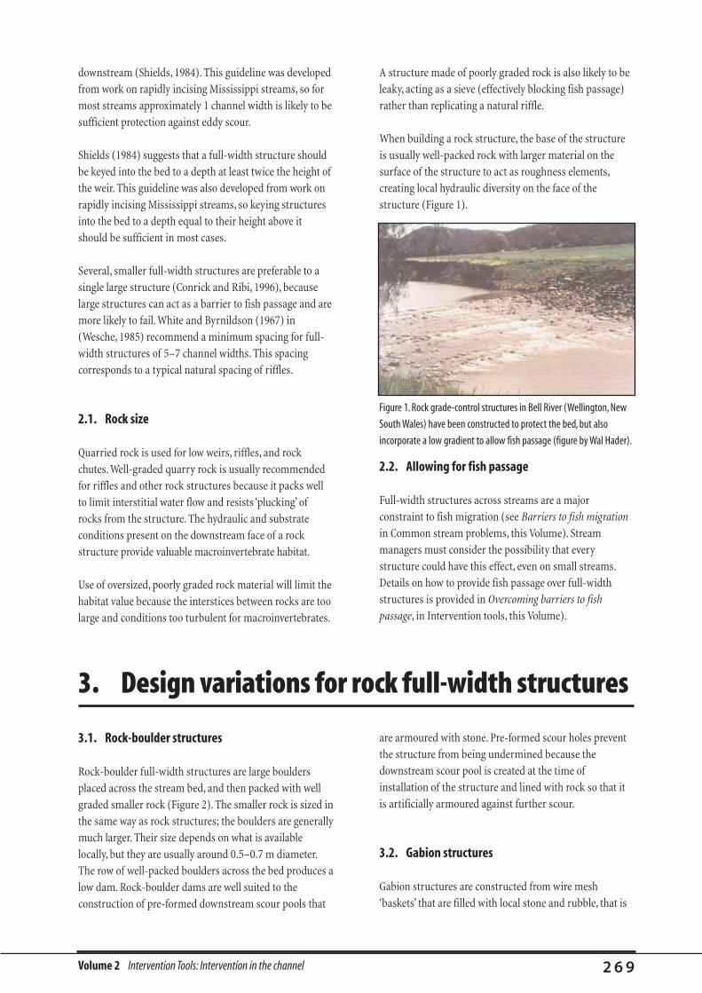
Volume 2 Intervention Tools: Intervention in the channel 2 6 9
downstream (Shields, 1984). This guideline was developed
from work on rapidly incising Mississippi streams, so for
most streams approximately 1 channel width is likely to be
sufficient protection against eddy scour.
Shields (1984) suggests that a full-width structure should
be keyed into the bed to a depth at least twice the height of
the weir. This guideline was also developed from work on
rapidly incising Mississippi streams, so keying structures
into the bed to a depth equal to their height above it
should be sufficient in most cases.
Several, smaller full-width structures are preferable to a
single large structure (Conrick and Ribi, 1996), because
large structures can act as a barrier to fish passage and are
more likely to fail. White and Byrnildson (1967) in
(Wesche, 1985) recommend a minimum spacing for full-
width structures of 5–7 channel widths. This spacing
corresponds to a typical natural spacing of riffles.
2.1. Rock size
Quarried rock is used for low weirs, riffles, and rock
chutes. Well-graded quarry rock is usually recommended
for riffles and other rock structures because it packs well
to limit interstitial water flow and resists ‘plucking’ of
rocks from the structure. The hydraulic and substrate
conditions present on the downstream face of a rock
structure provide valuable macroinvertebrate habitat.
Use of oversized, poorly graded rock material will limit the
habitat value because the interstices between rocks are too
large and conditions too turbulent for macroinvertebrates.
A structure made of poorly graded rock is also likely to be
leaky, acting as a sieve (effectively blocking fish passage)
rather than replicating a natural riffle.
When building a rock structure, the base of the structure
is usually well-packed rock with larger material on the
surface of the structure to act as roughness elements,
creating local hydraulic diversity on the face of the
structure (Figure 1).
Figure 1. Rock grade-control structures in Bell River (Wellington, New
South Wales) have been constructed to protect the bed, but also
incorporate a low gradient to allow fish passage (figure by Wal Hader).
3.1. Rock-boulder structures
Rock-boulder full-width structures are large boulders
placed across the stream bed, and then packed with well
graded smaller rock (Figure 2). The smaller rock is sized in
the same way as rock structures; the boulders are generally
much larger. Their size depends on what is available
locally, but they are usually around 0.5–0.7 m diameter.
The row of well-packed boulders across the bed produces a
low dam. Rock-boulder dams are well suited to the
construction of pre-formed downstream scour pools that
are armoured with stone. Pre-formed scour holes prevent
the structure from being undermined because the
downstream scour pool is created at the time of
installation of the structure and lined with rock so that it
is artificially armoured against further scour.
3.2. Gabion structures
Gabion structures are constructed from wire mesh
‘baskets’ that are filled with local stone and rubble, that is
3. Design variations for rock full-width structures
2.2. Allowing for fish passage
Full-width structures across streams are a major
constraint to fish migration (see Barriers to fish migration
in Common stream problems, this Volume). Stream
managers must consider the possibility that every
structure could have this effect, even on small streams.
Details on how to provide fish passage over full-width
structures is provided in Overcoming barriers to fish
passage, in Intervention tools, this Volume).

Volume 2 Intervention Tools: Intervention in the channel 2 7 0
often relocated from a point bar. They are quite time-
consuming to build and the life of the gabion mesh is
limited to about 10 years (House, 1996), but they have the
advantage of enabling designers to shape dams according
to their needs. Gabion dams have the added benefit of
requiring little heavy equipment for construction, although
they are much easier to build if a front-end loader can be
used to fill the gabion basket and excavate the bed. Gabion
dams probably find their best application in wide, shallow
streams that have abundant coarse gravels (Wesche, 1985).
Cobble of around 0.1 m diameter is suitable for gabions, and
special wire mesh that is easy to form into the baskets is
also available (Wesche, 1985). The following design tips for
gabion construction come from successful rehabilitation of
a coastal stream in Oregon, USA (House, 1996).
• Gabions were anchored to the stream bed by driving
1.2 m steel rebar (metal rod used in reinforced
concrete) through the gabion dam into the stream bed.
• A cable was threaded through the gabion baskets before
filling, and anchored to deadmen on each bank.
• Gabions were keyed 1–5 m into the banks.
• To prevent outflanking, gabions were riprapped
immediately upstream and downstream of where they
were connected to the banks.
The limited life of gabion structures is probably the reason
they are not used more often. Remember the golden rule
for instream structures—if the system is not changed
permanently even after the structure has failed then it is
not a successful technique. This means gabion structures
should probably be limited to applications where the
gabion material will be stabilised by vegetation such that
the structures will not be destroyed after corrosion of the
wire baskets.
3.3. Riffles
Artificial riffles are rock structures designed to replicate
natural riffle formations (Figure 3). They are a common
habitat enhancement technique because they produce
upstream pools, and are designed to allow fish passage.
Artificial riffles can also act as a bed control structure like
traditional rock chutes. A well-designed grade control
structure made from rock should incorporate the fish
passage capabilities of riffles.
An example of the application of artificial riffles for bed
control and habitat enhancement is shown in Figure 4.
Riffles were installed to create a backwater to protect the
cracking clays of the stream bed and banks, and to
enhance habitat by creating pools in this steep section of
stream (Figure 4). Although the riffles are much better that
the original clay channel, their design could be improved
by rectifying the following problems:
• the rock material is of a uniform large size, so the riffles
are very porous and there is not a full-height backwater
behind the structure;
• the riffles do not completely armour the bed (ie. not
enough rock is used) so the bed is scouring from flow
between the rocks; and
• the riffles are not keyed into the bed or banks.
Figure 2. Rock-boulder structures on Eastern Creek (Sydney) (by Wal
Hader).
Figure 3. A natural riffle in the Campaspe River,Victoria.
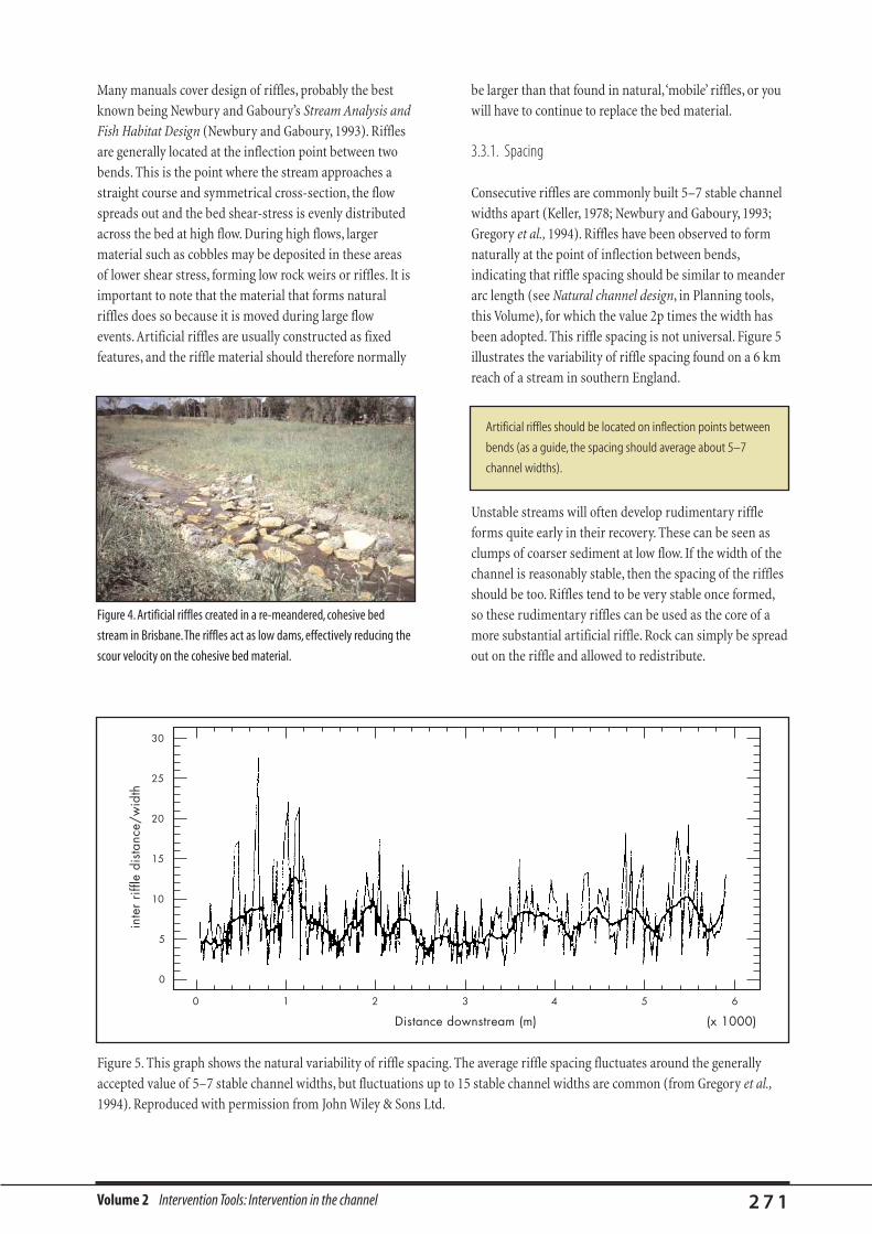
Volume 2 Intervention Tools: Intervention in the channel 2 7 1
Many manuals cover design of riffles, probably the best
known being Newbury and Gaboury’s Stream Analysis and
Fish Habitat Design (Newbury and Gaboury, 1993). Riffles
are generally located at the inflection point between two
bends. This is the point where the stream approaches a
straight course and symmetrical cross-section, the flow
spreads out and the bed shear-stress is evenly distributed
across the bed at high flow. During high flows, larger
material such as cobbles may be deposited in these areas
of lower shear stress, forming low rock weirs or riffles. It is
important to note that the material that forms natural
riffles does so because it is moved during large flow
events. Artificial riffles are usually constructed as fixed
features, and the riffle material should therefore normally
be larger than that found in natural,‘mobile’ riffles, or you
will have to continue to replace the bed material.
3.3.1. Spacing
Consecutive riffles are commonly built 5–7 stable channel
widths apart (Keller, 1978; Newbury and Gaboury, 1993;
Gregory et al., 1994). Riffles have been observed to form
naturally at the point of inflection between bends,
indicating that riffle spacing should be similar to meander
arc length (see Natural channel design, in Planning tools,
this Volume), for which the value 2p times the width has
been adopted. This riffle spacing is not universal. Figure 5
illustrates the variability of riffle spacing found on a 6 km
reach of a stream in southern England.
Artificial riffles should be located on inflection points between
bends (as a guide, the spacing should average about 5–7
channel widths).
(x 1000)Distance downstream (m)
inte
r rif
fle d
ista
nce/
wid
th
0
0 1 2 3 4 5 6
5
10
15
20
25
30
Figure 5. This graph shows the natural variability of riffle spacing. The average riffle spacing fluctuates around the generally
accepted value of 5–7 stable channel widths, but fluctuations up to 15 stable channel widths are common (from Gregory et al.,
1994). Reproduced with permission from John Wiley & Sons Ltd.
Figure 4. Artificial riffles created in a re-meandered, cohesive bed
stream in Brisbane.The riffles act as low dams, effectively reducing the
scour velocity on the cohesive bed material.
Unstable streams will often develop rudimentary riffle
forms quite early in their recovery. These can be seen as
clumps of coarser sediment at low flow. If the width of the
channel is reasonably stable, then the spacing of the riffles
should be too. Riffles tend to be very stable once formed,
so these rudimentary riffles can be used as the core of a
more substantial artificial riffle. Rock can simply be spread
out on the riffle and allowed to redistribute.
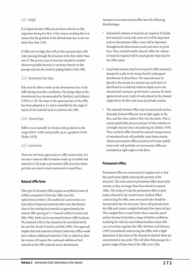
Volume 2 Intervention Tools: Intervention in the channel 2 7 2
3.3.2. Height
It is important that riffles do not form a barrier to fish
migration during low flow. A first step in avoiding this is to
ensure that the gradient of the downstream face is not too
steep (less than 1:20).
If riffles are too high, they will act like a porous dam, with
water passing through the structure at low flow rather than
over it. This porous type of structure should be avoided
wherever possible because it can form a barrier to fish
passage and can also result in piping failure of the riffle.
3.3.3. Downstream face slope
Fish must be able to swim up the downstream face of the
riffle during most flow conditions. The design slope of the
downstream face recommended by Newbury and Gaboury
(1993) is 1:20. The slope of the upstream face of the riffle
has been adopted as 4:1 and is controlled by the angle of
repose of the material used to construct the riffle.
3.3.4. Channel slope
Riffles occur naturally in streams with gradients in the
range 0.0015–0.005 and possibly up to a gradient of 0.01
(Keller, 1978).
3.3.5. Construction
There are two basic approaches to riffle construction: (a)
recreate a natural riffle formation made up of mobile bed
material; or (b) make a permanent riffle structure where
particles are sized to resist movement in most flows.
Natural riffle form
This type of recreated riffle requires an artificial source of
cobbles and gravel to form the riffles (see Bed
replenishment, below). The method of construction is to
leave piles of imported material with a size distribution
close to the existing bed material, at approximately the
natural riffle spacing of 5–7 channel widths (Conrick and
Ribi, 1996). Pools can be excavated between riffle locations.
The material is left in the channel to be smoothed out by
the next few floods (Conrick and Ribi, 1996). This approach
implies that bed material is limited (otherwise riffles would
form without additional material). If this is indeed so, then
the stream will require the continued addition of bed
material as the riffle material moves downstream.
Attempts to recreate natural riffles have the following
disadvantages.
• Substantial volumes of material are required. If mobile
bed material is used, only some of it will be deposited
to form downstream riffles; some will be deposited
throughout the downstream pools and some on point
bars. Thus, to build mobile ‘natural’ riffles the volume
of material required will be much greater than that for
the riffles alone.
• Local bank erosion may be increased if riffle material is
dumped in a pile in the stream bed for subsequent
distribution by flood flows. The material must be
placed in the stream in a natural way, such that it is
distributed to a relatively uniform depth across the
channel and continues up the bank to armour the bank
against local scour. A pile of rocks placed in the channel
might divert the flow and cause local bank erosion.
• The naturally formed riffles may increase bank erosion.
Naturally formed riffles are not at right angles to the
flow, and they thus redirect flow into the banks. This is
a quite predictable process and part of the evolution of
a straight channel into a meandering one (Keller, 1978).
Thus, artificial riffles formed by natural transportation
of introduced rock will probably cause bank erosion,
whereas permanent riffles (constructed of non-mobile
sized rock) will probably not (permanent riffles are
orientated at right angles to the flow).
Permanent riffles
Permanent riffles are constructed of angular rock so that
they pack more tightly, reducing the porosity of the
structure. The rocks used on permanent riffles must resist
erosion, so they are larger than those found on natural
riffles. The sizing of rocks for permanent riffles is most
easily achieved by the tractive stress method.When
constructing the riffle, some oversized rocks should be
incorporated into the structure. These will protrude from
the riffle and create a complex hydraulic flow down its face.
This complex flow is much better than a smooth, paved
surface because it provides a range of habitat conditions,
including low velocity areas behind boulders where fish
can rest as they negotiate the riffle. Newbury and Gaboury
(1993) recommend constructing the riffles with a slight
depression in the centre of the channel so that low flows are
concentrated at one point. This will allow fish passage for a
greater range of flows than if the riffle crest is flat.

Volume 2 Intervention Tools: Intervention in the channel 2 7 3
An example of riffleconstruction fromMink Creek inManitoba CanadaPresented in Newbury and Gaboury (1993)
Hamilton Creek and its tributaries in Manitoba, Canada, were
channelised in the 1950s to improve agricultural drainage and
reduce spring flooding.The stream channels were straightened
and uniformly graded to increase their discharge capacity for
higher run-off peaks from the increasingly cleared catchment.
Sediment from the stream discharged into a shallow
downstream lake. As a consequence of the channelisation of
Mink Creek and other tributaries, sediment input to the lake
filled it to one quarter of its mean depth (0.8 m) over the
period 1959–1980, and fish catch from the lake has dropped to
5–10% of its pre-1950 level.The goal of the Mink Creek
rehabilitation project is to recreate the natural biological
habitat with a view to increasing the fish population.The
channelised stream lacks pool and riffle habitat required for
walleye trout spawning, and has an increased slope and poor
instream hydraulic diversity.
The approach to rehabilitating this reach was to construct
artificial riffles in the channel, based on the spacing of riffles in
the original channel.The original stream characteristics were
compiled from early surveys, air photographs and the
recollections of local fishermen and farmers. Natural spawning
riffles for walleye were also studied. (See Natural channel
design, in Planning tools, this Volume, for more advice on how
to develop a template for your rehabilitation project.)
To achieve the pool depths, riffle gradients and flow diversity
observed in the template site, the riffle crests were set to follow
the average slope of the stream segment.The maximum slope of
the downstream face of the riffles was 5% (20:1),and riffle
material was sized on the basis of tractive stress at the riffle—
calculated for bankfull flow and for when flow was a critical
height over the riffle. In several cases the riffles were located at the
same location as the riffles had occurred before channelisation
and,on average,the riffles were spaced at 6.4 times the pre-
channelisation channel width.Riffle crests were elevated from 0.5
to 0.8 m (average 0.6 m) above the channel bottom to create
pools that extended to the mid-point of the upstream riffle slope
(ie.net drop of 0.3 m at each riffle) (see Figures 6 and 7).
NATURAL SPAWNING RIFFLE - BED PROFILE
Metres
FLOW
SEC. A-A
SEC. B-B
0
1.0
2.0
(A)
(B)
A A
20:1
FIELDSTONE FILL TYPICAL FIELDSTONERIFFLE PLAN
AND SECTION4:1
0.9m 0.6m
0.6m4:1
20:1
"V" SHAPED CREST
B
B
10 20 30 40 50
Met
res
6m B
ASE
Figure 6. Profiles of natural riffles and design details for artificial riffles constructed in Mink Creek, Manitoba, Canada (Newbury and Gaboury,
1993). Reproduced with permission from Newbury Hydraulics Ltd.
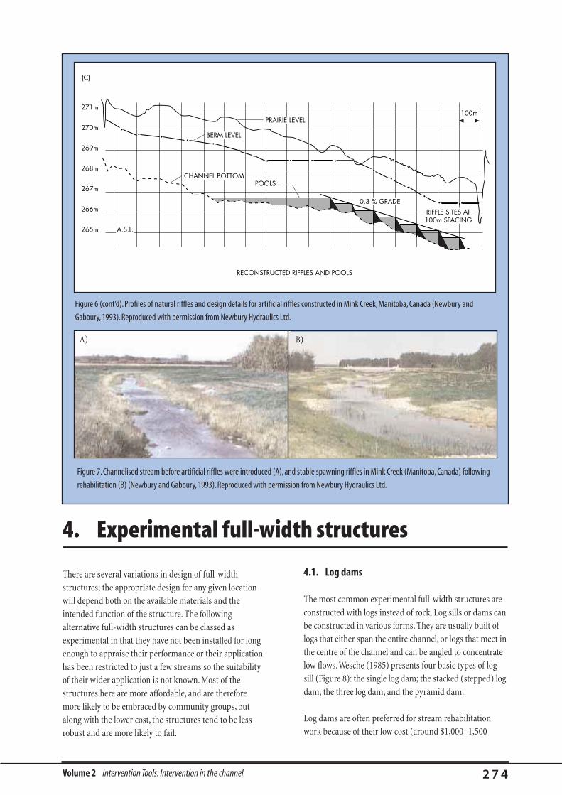
Volume 2 Intervention Tools: Intervention in the channel 2 7 4
Figure 6 (cont’d). Profiles of natural riffles and design details for artificial riffles constructed in Mink Creek, Manitoba, Canada (Newbury and
Gaboury, 1993). Reproduced with permission from Newbury Hydraulics Ltd.
Figure 7. Channelised stream before artificial riffles were introduced (A), and stable spawning riffles in Mink Creek (Manitoba, Canada) following
rehabilitation (B) (Newbury and Gaboury, 1993). Reproduced with permission from Newbury Hydraulics Ltd.
There are several variations in design of full-width
structures; the appropriate design for any given location
will depend both on the available materials and the
intended function of the structure. The following
alternative full-width structures can be classed as
experimental in that they have not been installed for long
enough to appraise their performance or their application
has been restricted to just a few streams so the suitability
of their wider application is not known. Most of the
structures here are more affordable, and are therefore
more likely to be embraced by community groups, but
along with the lower cost, the structures tend to be less
robust and are more likely to fail.
4.1. Log dams
The most common experimental full-width structures are
constructed with logs instead of rock. Log sills or dams can
be constructed in various forms. They are usually built of
logs that either span the entire channel, or logs that meet in
the centre of the channel and can be angled to concentrate
low flows.Wesche (1985) presents four basic types of log
sill (Figure 8): the single log dam; the stacked (stepped) log
dam; the three log dam; and the pyramid dam.
Log dams are often preferred for stream rehabilitation
work because of their low cost (around $1,000–1,500
4. Experimental full-width structures
(C)
271m
RECONSTRUCTED RIFFLES AND POOLS
100m
270m
269m
268m
267m
266m
265m
CHANNEL BOTTOM
BERM LEVEL
PRAIRIE LEVEL
POOLS
0.3 % GRADERIFFLE SITES AT100m SPACING
A.S.L.
A) B)

Volume 2 Intervention Tools: Intervention in the channel 2 7 5
(Allan Raine, personal communication)) and natural
appearance. Log sills are more prone to failure than rock
full-width structures because the downstream face of the
log sill is steeper, and energy dissipation thus occurs in the
scour pool. Even steep-faced rock weirs provide some
energy dissipation down the face of the weir. The failure of
log sills by undermining due to expansion of the scour
pool is even more prevalent if the flows are concentrated,
such as with Schauberger sills (see section 4.2, below).
Below are two important requirements in designing and
installing a log dam.
1. Provide protection against undercutting from scour
under the structure. In areas where the bed material is
not coarse enough to form an armouring layer, use rock
to form an armoured, pre-formed scour hole. Protect
from undercutting by piping under the sill, or by using
geotextile to seal the weir (Shields, 1984). Note that the
dam in Figure 9 did not incorporate geotextile or a pre-
formed scour pool. The success of this example is
probably because of the wide, level sill that did not
concentrate flow, so that scour formation occurred
across the whole bed. The upstream pool quickly filled
with bedload, limiting the potential for piping failure
under the structure.
Figure 8. Basic log dam configurations (from Wesche, 1985). Reproduced with permission from Butterworth Publishing.
Single Log Dam
Stacked Log Dam
Three Log Dam
Pyramid Dam
Side
Side End
End
Side End
Side End
Figure 9. A flat-crested log dam on Taylors Arm, a tributary of the
Nambucca River in New South Wales (photo by Allan Raine).
2. To prevent outflanking, anchor log sills at least 1.2–1.8 m
into ‘non-mobile’ bank material (Wesche, 1985).
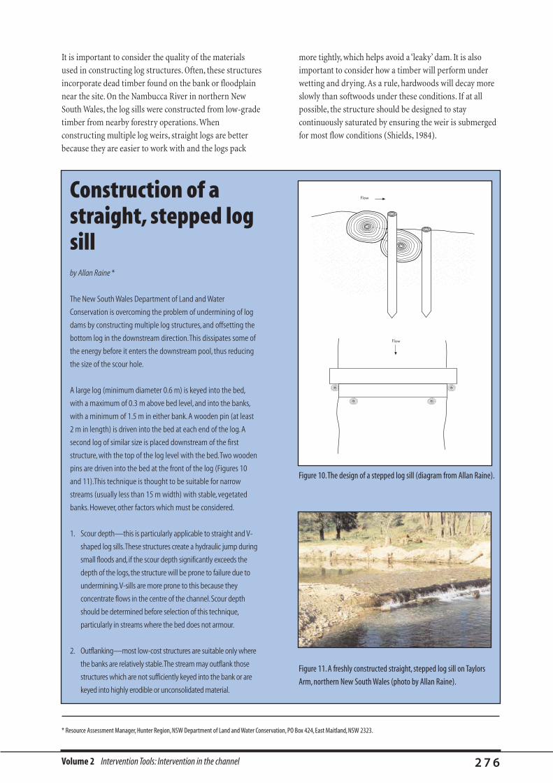
Volume 2 Intervention Tools: Intervention in the channel 2 7 6
It is important to consider the quality of the materials
used in constructing log structures. Often, these structures
incorporate dead timber found on the bank or floodplain
near the site. On the Nambucca River in northern New
South Wales, the log sills were constructed from low-grade
timber from nearby forestry operations. When
constructing multiple log weirs, straight logs are better
because they are easier to work with and the logs pack
more tightly, which helps avoid a ‘leaky’ dam. It is also
important to consider how a timber will perform under
wetting and drying. As a rule, hardwoods will decay more
slowly than softwoods under these conditions. If at all
possible, the structure should be designed to stay
continuously saturated by ensuring the weir is submerged
for most flow conditions (Shields, 1984).
Construction of astraight, stepped logsillby Allan Raine *
The New South Wales Department of Land and Water
Conservation is overcoming the problem of undermining of log
dams by constructing multiple log structures, and offsetting the
bottom log in the downstream direction.This dissipates some of
the energy before it enters the downstream pool, thus reducing
the size of the scour hole.
A large log (minimum diameter 0.6 m) is keyed into the bed,
with a maximum of 0.3 m above bed level, and into the banks,
with a minimum of 1.5 m in either bank.A wooden pin (at least
2 m in length) is driven into the bed at each end of the log. A
second log of similar size is placed downstream of the first
structure, with the top of the log level with the bed.Two wooden
pins are driven into the bed at the front of the log (Figures 10
and 11).This technique is thought to be suitable for narrow
streams (usually less than 15 m width) with stable, vegetated
banks. However, other factors which must be considered.
1. Scour depth—this is particularly applicable to straight and V-
shaped log sills.These structures create a hydraulic jump during
small floods and, if the scour depth significantly exceeds the
depth of the logs, the structure will be prone to failure due to
undermining.V-sills are more prone to this because they
concentrate flows in the centre of the channel.Scour depth
should be determined before selection of this technique,
particularly in streams where the bed does not armour.
2. Outflanking—most low-cost structures are suitable only where
the banks are relatively stable.The stream may outflank those
structures which are not sufficiently keyed into the bank or are
keyed into highly erodible or unconsolidated material.
* Resource Assessment Manager, Hunter Region, NSW Department of Land and Water Conservation, PO Box 424, East Maitland, NSW 2323.
Figure 10.The design of a stepped log sill (diagram from Allan Raine).
��������������������������������
Flow
Flow
Figure 11. A freshly constructed straight, stepped log sill on Taylors
Arm, northern New South Wales (photo by Allan Raine).

Volume 2 Intervention Tools: Intervention in the channel 2 7 7
4.2. Schauberger sills
The following information on European grade-control
structures was supplied by Wal Hader (New South Wales
Department of Land and Water Conservation).
Schauberger sills are built from either logs or, less
frequently, rocks. The sill is V-shaped, with the apex of
the V pointing upstream. The two arms are also sloped
from the bank end into the stream, so that the apex of the
sill is the lowest point, corresponding with the thalweg of
the channel. Thus, in cross-section a Schauberger sill
looks like a gentle V-notch weir. Low flows are
concentrated in the centre of the structure, providing
maximum depth of water for fish passage. The upstream
orientation of the two arms of the Schauberger sill also
concentrates flows in the centre of the channel (Figure
12). This maintains a large scour pool downstream of the
sill. This is excellent for fish habitat, but may also result
in the structure being undermined. The potential for
undermining is particularly high when the bed material
is not coarse enough to produce an armouring layer to
maintain the scour hole size.
Figure 12.A Schauberger sill (flow from left to right).Note that the apex
of the sill is the lowest point, and is pointing upstream.As a result, the
flow is concentrated in the centre of the channel, and there is a deep
scour pool downstream of the structure (photo by Wal Hader).
Figure 13. An example of a Mangfall sill with a central fishway (photo
by Wal Hader).
4.3. Mangfall sills
Mangfall sills were developed in Germany by the Bavarian
Water Authority. The crest is constructed in a series of
arches, one of which can incorporate a fishway. The
abutment boulders of the arches are supported by piles. A
scour bed of boulders is provided immediately
downstream of the crest. The arches concentrate flow and
restrict low flow to the central fishway (Figure 13). The
fishway finishes level with the base of the structure. This is
a preferred condition when designing for fish passage,
because fish can more easily find the fishway if all
discharge occurs at the same cross section. The height of
the Mangfall sill drop is dependent on the size of boulders
available for constructing the sill crest. The plunge pools
immediately below the sill crests should be armoured with
rock keyed into the bed.

Volume 2 Intervention Tools: Intervention in the channel 2 7 8
Partial-width structures are usually employed to stabilise
the bank by moving the attack point to a hard structure,
or by moving the thalweg of the stream away from
eroding banks. There are many additional applications of
partial-width structures such as for realigning the
channel (as for overwide channels), creating a narrower,
deeper, low-flow channel, or creating local scour and
depositional features to enhance the rehabilitation of the
in-stream habitat.
As a general rule, the following outcomes can be expected
when using partial-width structures.
• Reduced sediment load to streams by protecting
eroding banks and storing sediment in the
embayments between structures.
• The construction material provides a substrate, and
gaps between the substrate (interstices) provide habitat
for macroinvertebrates.
• Hydraulic diversity is increased through the formation
of scour pools at the tip of partial-width structures.
• Low-flow water depths are increased by narrowing the
channel, and a low velocity zone behind the structures
can create conditions suitable for revegetation and
long-term stability of the bank.
• Varied hydraulic conditions create downstream bars
which, depending on the bed material of the stream,
may expose spawning gravels required by some native
species.
PARTIAL-WIDTH BANK EROSION CONTROLSTRUCTURES
This section provides details about how to maximise the
environmental benefit of partial-width structures that are
commonly used. Alternative partial-width structures are
provided in the next section, on experimental partial-
width structures.
1.1. Groynes
Groynes are stream management structures used to stop
bank erosion and train the channel. They are built to abut
into the stream channel from an eroding bend, at around
90° to the stream flow. Their main function is to reduce
water velocities and shear stress in the vicinity of the
eroding bank. The creation of lower velocities and shear
stress on the outside bank reduces erosion and can
create conditions suitable for deposition of sediment if
the flow velocities are low enough.
Groynes are an erosion control tool: the benefits for
stream rehabilitation are a constrained low-flow channel
and localised bed scour features. Similar or better
stream-habitat enhancement results can be achieved
more cost-effectively with other partial-width
structures, so groynes are not covered in detail in this
manual. There are various design manuals for groynes,
the most commonly referred to in Australia being the
‘Guidelines for Stabilising Waterways’ (Working Group
on Waterway Management, 1991).
1. Tried and true partial-width structures
The difference between retards and groynesThere is often confusion in terminology between retards and groynes. Retards are permeable structures, and are usually lower than groynes.This
confusion has led to the incorrect naming of structures such as brush groynes and pin groynes, which are in fact types of retards.

Volume 2 Intervention Tools: Intervention in the channel 2 7 9
1.2. Traditional retards
Retards are permeable structures used for bank
stabilisation and/or river training. Because they are
relatively cheap and effective, they are a common erosion
control and channel alignment tool. Traditional retards are
a series of piles which extend from the bank toward the
centre of the channel. Cross members may be attached to
create a permeable barrier to flow (Figure 14). Retards are
designed for erosion control; they are usually constructed
on an artificial bench (often referred to as a berm) on the
outside of eroding bends. The structures are intended to
reduce the erosion of the bank, maintain the stability of
the artificial bench, create low velocity conditions behind
the structure suitable for the establishment of vegetation
and to encourage deposition of fine sediment on the bench
to improve the moisture retention needed for revegetation
of the bench. The usual intention is that the vegetation will
ultimately stabilise the bench after the retard has
disintegrated (in 10–20 years).
Basic alternatives for retards are:
• timber or steel piles with horizontal rails;
• piles or posts supporting cables and wire mesh;
• lines of lightweight post-and-wire structures known as
‘jacks’;
• piles or posts supporting logs or brush (ie.‘brush retard,
see Experimental partial-width structures, below);
• open timber or steel pile structures without rails (ie.
‘pin retard, see Experimental partial-width structures,
below); and
• live tree cuttings supported by piles and cables
(Working Group on Waterway Management, 1991).
The main points to consider in the design of retards are
height, orientation, stability under bed scour conditions,
strength to withstand hydraulic forces and their porosity,
or percentage of retard open to flow.
A report by Dyer et al. (1995), based on field observations
and a flume study of retards, has improved our
understanding of the mechanisms by which they protect
banks, and has added some key design considerations for
their construction. The results of this study have been
included in a revised version of the retards and groynes
section of the ‘Guidelines for stream stabilisation’
(Drummond et al. 1995). The following are some
conclusions from the study that impact directly on retard
design:
• Vegetation establishment is a critical feature for long-
term stability of the artificial bench on which retards
are constructed.
• Fine sediment is collected in low spots on the artificial
bench, around the roots of trees (willows) and in grass
located on the bench, so the establishment of
vegetation will accelerate deposition.
• The height of the retard relative to the depth of flow is
important—retards are more effective at reducing
downstream velocities when they are submerged.
• Retard angle to the flow has little effect on the hydraulic
characteristics in the embayment behind the retard
(but see bendway weirs below).
• Retards do not cause major deflection across the
channel into the opposite bank; rather they retard flow
in the area of the retard and increase the velocity in the
rest of the stream cross-section.
• A reduced velocity behind the retard is observable for
up to 40 times the height of the retard (when tested in a
straight flume).
• The streamward end of retards should be steeply
angled downstream (45–30° to the flow) (ie. a small
hook placed on the end at this angle downstream) to
limit scour near the structure, and move the main
scour formation towards the centre of the channel.
• Maximum velocities for the stability of bed particles
behind retards have been verified; hence retards can be
designed on the basis of the maximum velocity
acceptable for the particle sizes on the artificial bench.
1.2.1. Where are retards used?
Retards are used mostly for narrowing and stabilising
over-wide streams. They are used for a range of stream
types, such as gravel bed streams (Figure 15), or rivers
with mostly fine, non-cohesive bed and bank material.
Where retards are used in attempts to increase local
deposition, it is important that there be a sediment supply

Volume 2 Intervention Tools: Intervention in the channel 2 8 0
to the reach. Where they are used simply as stabilisation
structures, they can be applied to practically any stream
but are unlikely to be successful in narrow, high energy,
incised streams.
1.2.2. Retards with alignment fences
Alignment fences can be built between retards the ends of
retards. They produce embayments which trap debris,
further reducing the flow velocities and encouraging
deposition (Conrick and Ribi, 1996). Alignment fences are
often used to protect vegetation planted on artificial
benches. Be warned that alignment fences are not
universally applicable and have failed at many sites
because they were washed out.
The construction of alignment fences depends on the
intensity of flow through the embayment. For fences that
are likely to be completely submerged, and subject to flow
velocities of the order of, say, 0.5 m/s or greater, fences
should be of sturdy design. An example of this type of
fence is made from steel railway lines driven into the
bench to approximately 2 m depth with heavy gauge wire
tightly connecting the posts, and galvanised mesh or
chainwire also tightly connected between the posts.
Benches such as those in the Wilson River example, which
are not likely to receive high velocity flows, could suffice,
with wooden posts firmly secured in place to say a depth
of 1 m, with lighter gauge wire and lighter mesh between
the posts.
������������������������������������������������������������
Approximate annual floodstage or bank height(which ever is less)
Extra rails may be used near the bank
Piles Rails 2/3
1/3 1mTypical
Figure 14.Traditional retard design (from Working Group on Waterway Management, 1991)
The following experimental partial-width structures are
mostly variations of groynes or retards. These are not
necessarily new concepts but include those that have
been tried at only a few sites or have not been fully
evaluated.
2.1. Pin retards
Pin retards consist of series of unconnected piles driven
into the stream bed to act as a retard. Pin retards have
been used in Victoria for some time and are currently
2. Experimental partial-width structures
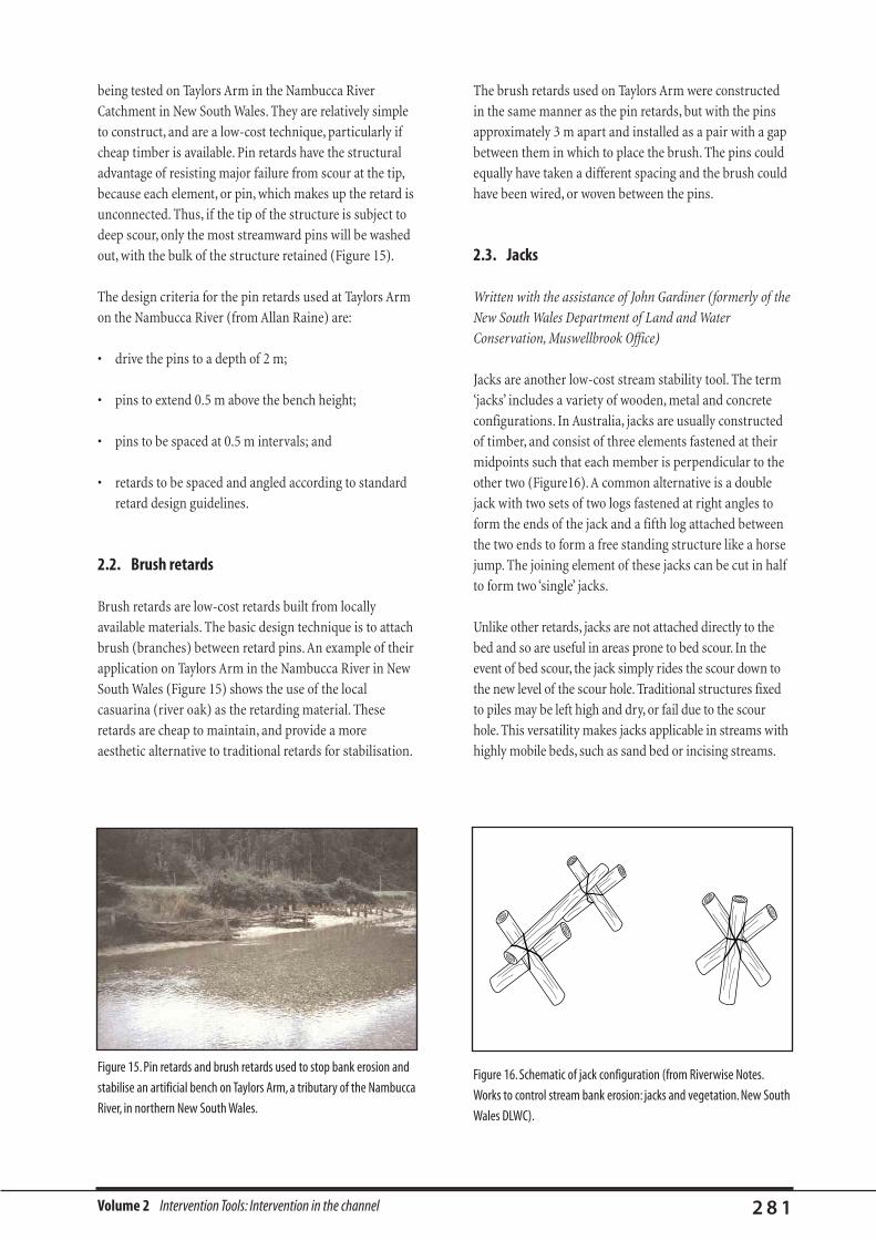
Volume 2 Intervention Tools: Intervention in the channel 2 8 1
being tested on Taylors Arm in the Nambucca River
Catchment in New South Wales. They are relatively simple
to construct, and are a low-cost technique, particularly if
cheap timber is available. Pin retards have the structural
advantage of resisting major failure from scour at the tip,
because each element, or pin, which makes up the retard is
unconnected. Thus, if the tip of the structure is subject to
deep scour, only the most streamward pins will be washed
out, with the bulk of the structure retained (Figure 15).
The design criteria for the pin retards used at Taylors Arm
on the Nambucca River (from Allan Raine) are:
• drive the pins to a depth of 2 m;
• pins to extend 0.5 m above the bench height;
• pins to be spaced at 0.5 m intervals; and
• retards to be spaced and angled according to standard
retard design guidelines.
2.2. Brush retards
Brush retards are low-cost retards built from locally
available materials. The basic design technique is to attach
brush (branches) between retard pins. An example of their
application on Taylors Arm in the Nambucca River in New
South Wales (Figure 15) shows the use of the local
casuarina (river oak) as the retarding material. These
retards are cheap to maintain, and provide a more
aesthetic alternative to traditional retards for stabilisation.
The brush retards used on Taylors Arm were constructed
in the same manner as the pin retards, but with the pins
approximately 3 m apart and installed as a pair with a gap
between them in which to place the brush. The pins could
equally have taken a different spacing and the brush could
have been wired, or woven between the pins.
2.3. Jacks
Written with the assistance of John Gardiner (formerly of the
New South Wales Department of Land and Water
Conservation, Muswellbrook Office)
Jacks are another low-cost stream stability tool. The term
‘jacks’ includes a variety of wooden, metal and concrete
configurations. In Australia, jacks are usually constructed
of timber, and consist of three elements fastened at their
midpoints such that each member is perpendicular to the
other two (Figure16). A common alternative is a double
jack with two sets of two logs fastened at right angles to
form the ends of the jack and a fifth log attached between
the two ends to form a free standing structure like a horse
jump. The joining element of these jacks can be cut in half
to form two ‘single’ jacks.
Unlike other retards, jacks are not attached directly to the
bed and so are useful in areas prone to bed scour. In the
event of bed scour, the jack simply rides the scour down to
the new level of the scour hole. Traditional structures fixed
to piles may be left high and dry, or fail due to the scour
hole. This versatility makes jacks applicable in streams with
highly mobile beds, such as sand bed or incising streams.
Figure 15. Pin retards and brush retards used to stop bank erosion and
stabilise an artificial bench on Taylors Arm, a tributary of the Nambucca
River, in northern New South Wales.
Figure 16. Schematic of jack configuration (from Riverwise Notes.
Works to control stream bank erosion: jacks and vegetation. New South
Wales DLWC).

Volume 2 Intervention Tools: Intervention in the channel 2 8 2
Jacks work by introducing a roughness element into the
flow. They are more porous than traditional retards and
are applied at closer spacing to achieve the required low
velocity conditions behind the structures. Jacks are
normally placed in an array along an artificial bench at
the toe of an eroding bank. The array is fastened
together by cable, and the jacks are usually anchored to
the bank by deadmen (buried logs attached to jacks with
a cable).
Jacks are extremely cheap structures for community
groups to build because no heavy machinery is usually
needed for their construction and installation (although
an excavator is required to form the artificial bench). The
jacks are not fixed to the bed so their placement and
alignment can be altered if initial placement is not
successful. When installed on sediment-starved streams
they are used to reduce the downstream flow velocity to
allow the establishment of vegetation rather than
encouraging deposition. In these cases, when deposition
has not occurred (ie. the jacks are not buried), the jacks
can be moved and reused on another eroding bend after
vegetation is suitably established.
Jacks are normally recommended for wide, shallow, silt or
sand-laden streams that are subject to severe scouring
during high-velocity flow (Department of Water
Resources, no date). Jacks have also been successfully used
in streams with larger bed material size.
A project on the Gloucester River near the town of
Gloucester (New South Wales) provides an example of the
application of jacks in streams with larger bed material. At
this point the Gloucester River has a catchment area of
260 km2, Q1.5 of 45 m3/s, bed slope of 0.0022 and a bed
material D50 of 6.75 cm. The site on the Gloucester River
was an area where gravel had been extracted, and where
the bank was rapidly eroding. The initial stabilisation
technique was to construct an artificial bench and use
retard fences. This technique failed (fences were washed
away, or destroyed). In 1992, jacks were installed by the
Gloucester Landcare group and the Department of Land
and Water Conservation as a trial to see how they would
perform in coarse bed material.
The area to be protected was 135 m long, and 37 jacks were
used; a combination of single (at the leading and trailing
Figure 17. Plan of works on the Gloucester River, northern New South Wales (figure by John Gardiner).The alignment is shown by the dashed line, and the
jacks are shown as .
������������������������������������������������������������
FLOW
JACKFIELD
ERODING
HIGH
BANK
RIVER
GRAVEL
GLOUCES
TER

Volume 2 Intervention Tools: Intervention in the channel 2 8 3
2.4. Low deflectors
Deflectors are any in-stream structure used to change the
direction of flow. For stream rehabilitation work, deflectors
are generally low structures that break the flow into
higher-velocity scour areas and low-velocity deposition
areas. The generally low profile of low deflectors ensures
their hydraulic effect is usually drowned out at bankfull
conditions (with the exception of ‘bendway weirs’, which
are covered in the next section). Hence, they provide
minimal bank protection, and their main purpose is to
create habitat.
Various configurations for low deflector are shown in
Figure 19 and described in the following section.
Submerged vanes are the most sophisticated type of
deflector, and are discussed in the following section.
Bendway weirs are low deflectors which are angled
upstream into the direction of flow. Design details for
bendway weirs are provided in section 2.6 below.
Straight deflectors are traditional, low deflectors angled
downstream at approximately 45° to the flow. They are
designed to create a scour pool at their tip and a bar
behind them (Hey, 1994).
Multiple deflectors can be double straight (V) and Y-
double deflectors, and are designed to create a scour pool
in the centre of the channel and bars behind the deflectors.
This application is preferred for streams without stable
banks. A-deflectors are designed to split the flow into two
scour channels and create a centre bar.
Wing deflectors are used in faster-flowing rivers, where a
separation zone or vortex can develop on the streamward
tip of straight deflectors. This separation zone and
associated flow expansion downstream of the low deflector
can cause bed scour and bank erosion. Wing deflectors are
designed to reduce the angle between the trailing edge and
flow direction, thus allowing a gradual downstream
expansion of flow that reduces the generation of
turbulence (Hey, 1994). Wing deflectors are essentially low
height, impermeable training arms, as mentioned in the
retards section.
2.4.1. Design tips for low deflectors
There are variations in design of low deflectors, depending
on the application and the availability of materials.
Generally, low deflectors are used in mid to low gradient
(slope less than 3%) over-wide gravel bed streams.
However, as a general rule the following deflector siting
criteria apply (adapted from a review in Wesche, 1985).
Figure 18. Jacks at the Gloucester River site, 5 years after installation.
Figure19. Alternative low deflector configurations, and the scour and deposition that they are likely to produce (from Stewardson et al., 1997). Reproduced
with permission from the Centre for Applied Environmental Hydrology.
����@@@@����ÀÀÀÀ����@@@@����ÀÀÀÀ��@@��ÀÀ��@@��ÀÀ�
�@@��ÀÀ��@@��ÀÀ����@@@@����ÀÀÀÀ����@@@@����ÀÀÀÀ
��@@��ÀÀ��@@��ÀÀ��@@��ÀÀ��@@��ÀÀ�@�À�@�À�@�À�@�À �@�À�@�À�@�À�@�À��
��@@@@����ÀÀÀÀ����@@@@����ÀÀÀÀSingle straight Bendway weir Double straight Y-double V-centreA-centre Double wingSingle wing
Flow
Bar Pool
��@@��ÀÀ��@@��ÀÀ
edge of the protection) and double jacks was used
(Figure 17). The jacks were made from timber-mill offcuts.
The outcome of this project is that, after a number of
floods, at least 2 m over the jacks, the artificial bench has
stabilised and native vegetation (and willows) are now
recolonising the artificial bench (Figure 18). This project
cost $10,000.
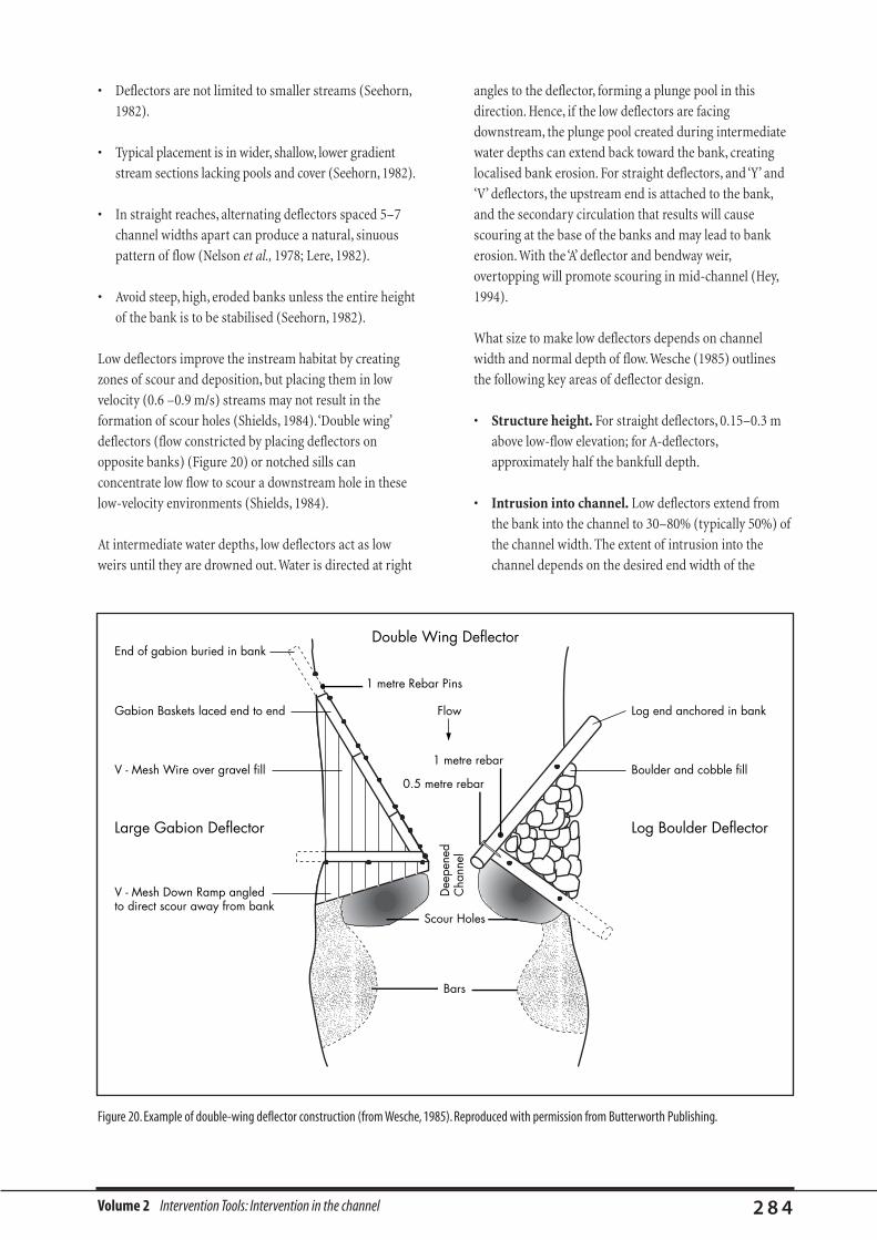
Volume 2 Intervention Tools: Intervention in the channel 2 8 4
• Deflectors are not limited to smaller streams (Seehorn,
1982).
• Typical placement is in wider, shallow, lower gradient
stream sections lacking pools and cover (Seehorn, 1982).
• In straight reaches, alternating deflectors spaced 5–7
channel widths apart can produce a natural, sinuous
pattern of flow (Nelson et al., 1978; Lere, 1982).
• Avoid steep, high, eroded banks unless the entire height
of the bank is to be stabilised (Seehorn, 1982).
Low deflectors improve the instream habitat by creating
zones of scour and deposition, but placing them in low
velocity (0.6 –0.9 m/s) streams may not result in the
formation of scour holes (Shields, 1984).‘Double wing’
deflectors (flow constricted by placing deflectors on
opposite banks) (Figure 20) or notched sills can
concentrate low flow to scour a downstream hole in these
low-velocity environments (Shields, 1984).
At intermediate water depths, low deflectors act as low
weirs until they are drowned out. Water is directed at right
angles to the deflector, forming a plunge pool in this
direction. Hence, if the low deflectors are facing
downstream, the plunge pool created during intermediate
water depths can extend back toward the bank, creating
localised bank erosion. For straight deflectors, and ‘Y’ and
‘V’ deflectors, the upstream end is attached to the bank,
and the secondary circulation that results will cause
scouring at the base of the banks and may lead to bank
erosion. With the ‘A’ deflector and bendway weir,
overtopping will promote scouring in mid-channel (Hey,
1994).
What size to make low deflectors depends on channel
width and normal depth of flow. Wesche (1985) outlines
the following key areas of deflector design.
• Structure height. For straight deflectors, 0.15–0.3 m
above low-flow elevation; for A-deflectors,
approximately half the bankfull depth.
• Intrusion into channel. Low deflectors extend from
the bank into the channel to 30–80% (typically 50%) of
the channel width. The extent of intrusion into the
channel depends on the desired end width of the
Figure 20. Example of double-wing deflector construction (from Wesche, 1985). Reproduced with permission from Butterworth Publishing.������
@@@@@@
������
ÀÀÀÀÀÀ
������
@@@@@@
������
ÀÀÀÀÀÀ
������
@@@@@@
������
ÀÀÀÀÀÀ
������
@@@@@@
������
ÀÀÀÀÀÀ
Double Wing Deflector
Log Boulder DeflectorLarge Gabion Deflector
End of gabion buried in bank
Gabion Baskets laced end to end Log end anchored in bank
V - Mesh Wire over gravel fill Boulder and cobble fill
Scour Holes
1 metre Rebar Pins
Flow
1 metre rebar
0.5 metre rebar
Dee
pene
dC
hann
el
V - Mesh Down Ramp angledto direct scour away from bank
Bars

Volume 2 Intervention Tools: Intervention in the channel 2 8 5
channel (see Natural channel design, in Planning tools,
this Volume).
• Key structures into the bank. If deflectors are
constructed of logs, they should be anchored into the
bank by 1.2–1.8 m (Wesche, 1985) or until well into
non-mobile material. There is little value in anchoring
deflectors to mobile gravel bars.
• Bed anchoring. Low deflectors are usually fixed in
position by rebar (metal bar used for reinforcing
concrete), although steel fence posts for small steams,
or piles driven into the stream bed for larger streams,
are also suitable.
2.5. Submerged vanes
Submerged vanes are flow-training structures designed to
modify the flow pattern near the bed by generating a
secondary circulation in the flow (Hey, 1994). They have
the effect of redistributing flow and sediment transport
within the channel cross-section (Odgaard and Wang,
1991a). Both deposition and increased scour can be
achieved with submerged vanes by manipulating their
location and angle. In terms of increased scour they can be
used to create scour pools for habitat enhancement (Hey,
1994), and to erode and deepen channels for navigation
(Odgaard and Spoljaric, 1986). They can be used to protect
banks by disrupting the natural helical flow pattern which
causes erosion of the toe of the bank at bends (Odgaard
and Mosconi, 1987). Submerged vanes can also be used to
increase deposition, such as in artificial bench formation
at the toe of outside bends, or at the mouth of a cut-off
(Odgaard and Spoljaric, 1986). Further, they can be used to
promote deposition zones such as side bars, for re-
meandering of over-wide sand and gravel bed streams
(Stewardson et al., 1997).
Submerged vanes exercise their effect through the creation
of a secondary current induced by the vertical pressure
gradients between the flow on either side of the vane.
Because the vane is at an angle to the flow, a pressure
differential will be established between flow on either side
of it, in much the same way as a pressure differential
caused by wind flowing over an aircraft’s wing creates lift.
There is also a vertical pressure gradient which, on the
low-pressure side of the vane (downstream) increases
from top to bottom, and decreases from top to bottom on
the high-pressure side (upstream). The combined effect of
the horizontal and vertical pressure gradients is a helical
motion of flow downstream of the vane. This downstream
spiral motion causes bed profile changes in a fashion
similar to helical flow in bends.
Submerged vanes have several applications: small local
variations in bed form can be created by single or double
vanes, while larger scale channel bed changes can be
instigated by vane fields made up of parallel formations
called vane arrays (Figure 21). The effectiveness of an
array depends on the number, spacing and dimensions of
the vanes.
Single, symmetrical and asymmetric vanes can be used to
produce local scour and bar formation. They are applied in
much the same way as deflectors, with the exception that
the vanes are not attached to the bank. The general effect
of vane arrays is to scour pools on the high-pressure
(upstream) side of the array, and bars on the low-pressure
(downstream) side.
Submerged vanes have not (to the knowledge of the
authors) been used for sediment management in
Australia, and have had only limited application for bank
protection in the United States. Current information
indicates that the angle of the vanes is critical to their
success, and that the margin for error is small. Submerged
��@@��ÀÀ��@@��ÀÀ��@@��ÀÀ��@@��ÀÀSingle short Single long Symmetrical Asymmetrical Vane array Vane field
Flow
Bar Pool
�@�À�@�À��@@��ÀÀ��@@��ÀÀ ��@@��ÀÀ��@@��ÀÀ��@@��ÀÀ��@@��ÀÀ�@�À�@�À
Figure 21. Alternative configuration of submerged vanes, and the scour and deposition that they produce (from Stewardson et al., 1997). Reproduced with
permission from the Centre for Applied Environmental Hydrology.

Volume 2 Intervention Tools: Intervention in the channel 2 8 6
vanes may therefore require some form of adjustment
after installation. Constructing vanes which are robust
enough to withstand the hydraulic forces and can be
adjusted poses a challenging design problem for stream
managers.
2.5.1. Where can submerged vanes be used?
Submerged vanes are suitable for a range of applications,
but are particularly useful in low-energy streams (Hey,
1994) such as lowland sand and gravel bed rivers
(Stewardson et al., 1997). Hey (1994) suggests that
submerged vanes are not well suited to high-energy
streams, such as upland rivers, and recommends that more
substantial rock structures be used for maintaining
channel morphology at high energy sites.
One of the advantages of submerged vanes, demonstrated
in flume experiments, is that they do not cause a net
change in the cross-sectional area of the channel or the
longitudinal slope of the water surface. This implies that
submerged vanes locally redistribute sediment but do not
affect the overall sediment budget of the reach (Odgaard
and Wang, 1991b). Other channel alignment methods
(retards) are based on trapping sediment to prevent it
from influencing downstream channel morphology. A
detailed design procedure for vane arrays is presented in
Odgaard and Wang (1991b).
In conclusion, vanes are potentially a powerful tool for
stabilising streams and creating artificial habitat, but they
are complex hydraulic structures that require detailed
design and, for the present, must be considered as
experimental.
2.6. Bendway weirs
Bendway weirs are not weirs at all, but low height
deflectors that are unusual in that they are angled
upstream (into the flow). This is in contrast to most
retards that tend to be higher, and to be angled
downstream (with the flow). Bendway weirs are reputed to
protect eroding banks by interrupting secondary
circulation (similar to vanes), and by deflecting flow away
from the eroding bank. For most angles of interception,
water will leave a sill at 90° degrees to the crest. Therefore,
if a deflector is angled upstream, flow is diverted toward
the centre of the channel.
The information in this section comes from unpublished
reports produced by David Derrick (US Army Engineer
Waterways Experiment Station,Vicksburg). Bendway weirs
are a quite new stream management tool, conceived in
1988, and only recently tested in New South Wales by the
Department of Land and Water Conservation. This section
is concerned with the use of bendway weirs for erosion
control and habitat enhancement in non-navigable
streams. In non-navigable streams, bendway weirs are
normally emergent during low flows, angled between 80
and 65° (to the flow direction) upstream, usually slope
from the bank into the stream and are constructed of rock
or logs.
2.6.1. Where can you use bendway weirs?
There is limited information currently available for the
application of bendway weirs, and where they are
appropriate. They have been used in a range of stream
types (sand, gravel and clay bed), and in conjunction with
other stream stabilisation techniques, including
revegetation and Longitudinal Peaked Stone Toe
Protection (LSTP), and revegetation.
The literature does not suggest any particular locations
that may be unsuitable for the application of bendway
weirs, but they are usually not designed to extend the full
width of the channel, and would therefore be prone to
failure in unstable bed streams.
Do not install bendway weirs in streams that are actively
incising. Stabilise the bed first.
The erosion protection benefit of bendway weirs appears to
come from their dampening of the secondary circulation.
They will therefore be less effective for erosion control
where the secondary circulation is weak. Secondary
circulation is weak in very tight bends, where the ratio
between the radius of curvature and the channel width
(Rc/w) is less than 2, because the flow tends to short circuit
the bend and flow across the point bar, so there is not a
smooth flow as in a sweeping bend. Open bends (Rc/w > 4)
approach the conditions of a straight channel, the bed is
flatter and secondary circulation is not well established, so
bendway weirs are not likely to be as effective in open
bends as they are in sweeping bends (Rc/w ~ 3) .

Volume 2 Intervention Tools: Intervention in the channel 2 8 7
2.6.2. Design of bendway weirs
Derrick describes the design of bendway weirs as an "art
rather than a science". In general, bendway weirs are
angled to direct the flow away from the eroding bank and
into the next downstream weir. Here are the design steps
that can be gleaned from Derrick’s descriptions.
1. Draw the planform of the bend and identify its centroid.
2. Draw rays out from the centroid to act as guides for
design.
3. Select the length of weir that will constrict the channel
as much as is necessary (see below).
4. Position the first weir (the weir furthest upstream) at
the entrance to the bend, with an angle that will direct
flow roughly parallel to the bank. It is important not to
angle weirs too sharply into the oncoming flow, because
if the weir is close to parallel to the oncoming flow it
will act as a flow divider and split the flow, causing
erosion behind it. In general, the weirs will have an
angle that is less than 20 degrees to the rays projected
from the centroid (see Figure 22).
5. The second weir is positioned such that a line drawn
from perpendicular to the centre of the first weir
intercepts the centre of the second weir (Figure 22). The
same is true for each successive weir. This means that
the spacing of weirs is dependent on the radius of the
bend and angle of the weirs. For tight meander bends or
bends with a long arc radius (horseshoe bends) the
weirs will be spaced closer than for more gradual bends.
2.6.2.A. Length of bendway weirs
There are no specific guidelines for determining the
appropriate length of bendway weirs. Derrick suggests the
following factors:
• how far from the eroding bank the thalweg needs to be
moved;
• the width of water (percentage of cross-section) the
weirs need to control to be effective;
• how erodible the point bars appear to be; and
• how much the point bars could be safely eroded
without detrimental side effects .
Centroid
Radial
< 20¡
Flow
Flow
Flow
Low FlowChannel
Captured Flow
Uncontrolled Flow
Figure 22.The design of a bendway weir field, including alignment and spacing, and the redirection effect on the water (modified from Derrick, 1997).

Volume 2 Intervention Tools: Intervention in the channel 2 8 8
Four stream rehabilitation projects that Derrick has
designed use bendway weir length between 1/4 and 1/2 the
pre-rehabilitation channel width.
2.6.2.B. Height of bendway weirs
The heights of bendway weirs will be determined largely
by the materials at hand. Originally only stone was used,
and such weirs could be built to any height desired.
However, bendway weirs have successfully been
constructed of single and multiple logs, and of geotextile
socks filled with river sand. Bendway weirs are designed to
be overtopped, and it is claimed by Derrick that the
redirecting effect of bendway weirs is not drowned out at
high flow but rather that the weirs work best under such
high-energy conditions. For stream rehabilitation work it
is often advantageous to narrow the low-flow channel
width to provide increased water depth during periods of
low flow. Hence, it is recommended that, in over-wide
streams, bendway weirs be installed at a height higher
than the low-flow water depth.
2.6.2.C. Key bendway weirs into the bed and banks
Bendway weirs, like other in-stream structures, are at risk
of being outflanked if they are not keyed into the bed and
banks. The bank depth to which bendway weirs need to be
keyed depends on the erodibility of the bank material. As a
minimum, the most upstream and downstream bendway
weirs should be keyed into the bank and the bottom 1/3 of
the bank should be revetted to protect against eddy scour.
In order to stop failure by undercutting resulting from the
expansion of the downstream scour hole back under the
structure, it is important to key bendway weirs into the bed.
For low weirs which extend the full channel width, Shields
(1984) recommends keying them into the bed to a depth at
least twice their height. However, Derrick has shown that, for
single-log bendway weirs, it is adequate to bury
approximately half the log and leave the other half above the
bed level to act as the bendway weir. It is important that the
log is stable when keyed into the bed and banks.
2.6.2.D. Slope bendway weirs into the channel
Rock bendway weirs designed by Derrick feature crests
that slope into the stream. The slope usually adopted is a
30 cm drop from the bank to the stream end of the weir.
The crest is sloped to reduce the flow concentrations at the
bank end of the weir. For log bendway weirs, it is not
possible to effectively key the structure into the bed and
create a sloping crest, so in this case the bendway weirs
should be installed with a level crest.
2.6.2.E. Anchoring
For rock bendway weirs, hydraulic failure is most likely to
occur as the ‘washing’ of rocks from the weir, flattening the
structure. Logs are likely to be completely displaced
downstream or against the bank.
There are various methods for anchoring log structures to
the bed:
• screw type anchors;
• piles— timber or steel posts—driven into the bed;
• pins, usually of rebar (reinforcing bar), driven through
the log into the bed; and
• deadmen, which are solid objects (usually logs but
clean 200 litre drums have also been suggested) buried
in the bank and attached by cable to the object to be
anchored.
In sand and gravel streams, deadmen are likely to be the most
effective way to stabilise bendway weirs.
It is recommended that bendway weirs be dug down into the
stream bed to about half of their total height (eg. half of the
total diameter of the logs).
2.6.3. Australian application of bendway weirs
Bendway weirs have been used by the late John Gardiner
(DLWC) on Pappinbarra Creek, a tributary of the Hastings
River in New South Wales (Figure 23). Pappinbarra Creek
is a high-energy gravel bed stream that is prone to
widening and channel avulsion across the narrow
floodplain. This is a result of upstream straightening, and
clearing of the floodplain. Further widening of the channel
has been prevented using log toe protection, and bendway

Volume 2 Intervention Tools: Intervention in the channel 2 8 9
weirs have been used to confine the low-flow channel and
to move the thalweg from the outside of the bend to the
centre of the channel during high flows.
Figure 23. Bendway weirs used to move the thalweg from the bank to
the centre of the channel on Pappinbarra Creek, a tributary of the
Hastings River, in New South Wales.
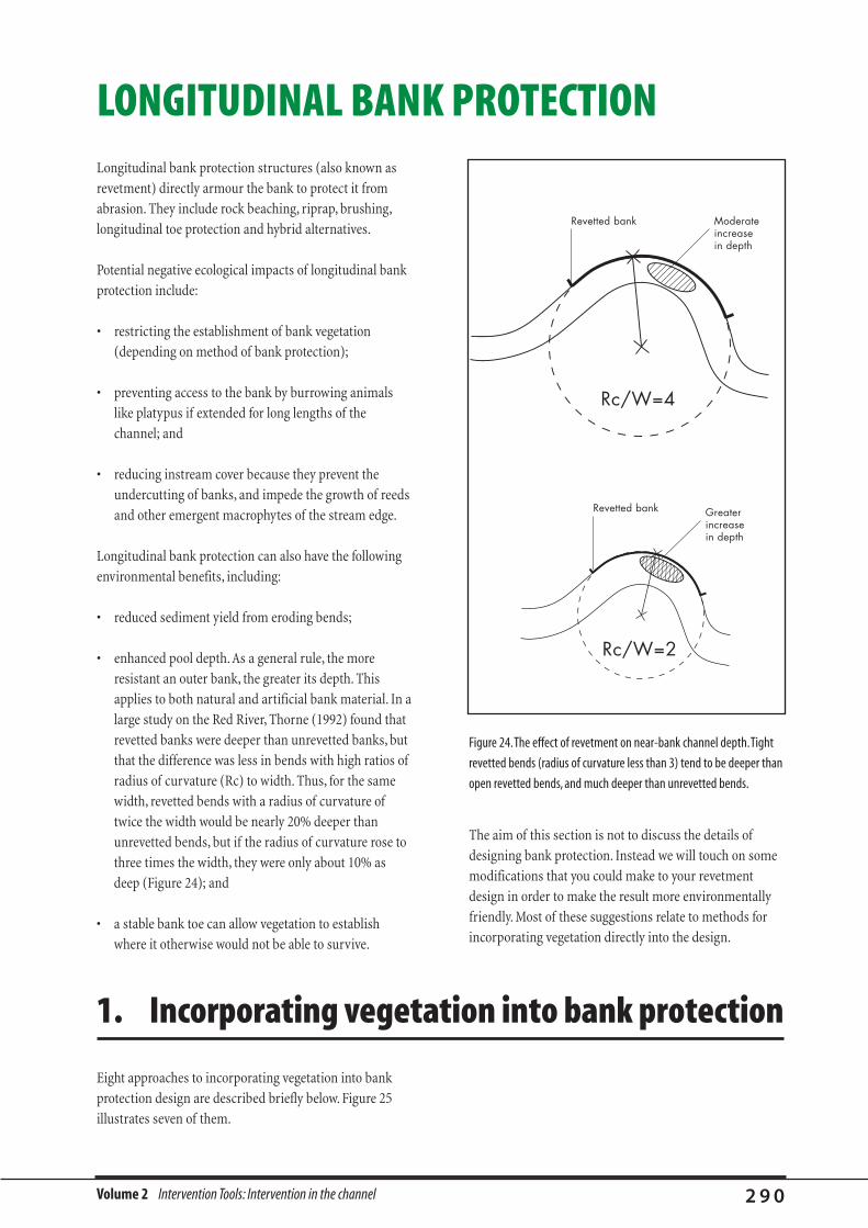
Volume 2 Intervention Tools: Intervention in the channel 2 9 0
Longitudinal bank protection structures (also known as
revetment) directly armour the bank to protect it from
abrasion. They include rock beaching, riprap, brushing,
longitudinal toe protection and hybrid alternatives.
Potential negative ecological impacts of longitudinal bank
protection include:
• restricting the establishment of bank vegetation
(depending on method of bank protection);
• preventing access to the bank by burrowing animals
like platypus if extended for long lengths of the
channel; and
• reducing instream cover because they prevent the
undercutting of banks, and impede the growth of reeds
and other emergent macrophytes of the stream edge.
Longitudinal bank protection can also have the following
environmental benefits, including:
• reduced sediment yield from eroding bends;
• enhanced pool depth. As a general rule, the more
resistant an outer bank, the greater its depth. This
applies to both natural and artificial bank material. In a
large study on the Red River, Thorne (1992) found that
revetted banks were deeper than unrevetted banks, but
that the difference was less in bends with high ratios of
radius of curvature (Rc) to width. Thus, for the same
width, revetted bends with a radius of curvature of
twice the width would be nearly 20% deeper than
unrevetted bends, but if the radius of curvature rose to
three times the width, they were only about 10% as
deep (Figure 24); and
• a stable bank toe can allow vegetation to establish
where it otherwise would not be able to survive.
LONGITUDINAL BANK PROTECTION
The aim of this section is not to discuss the details of
designing bank protection. Instead we will touch on some
modifications that you could make to your revetment
design in order to make the result more environmentally
friendly. Most of these suggestions relate to methods for
incorporating vegetation directly into the design.
Figure 24.The effect of revetment on near-bank channel depth.Tight
revetted bends (radius of curvature less than 3) tend to be deeper than
open revetted bends, and much deeper than unrevetted bends.
Revetted bank
Rc/W=4
Rc/W=2
Moderate increasein depth
Revetted bank Greater increasein depth
Eight approaches to incorporating vegetation into bank
protection design are described briefly below. Figure 25
illustrates seven of them.
1. Incorporating vegetation into bank protection
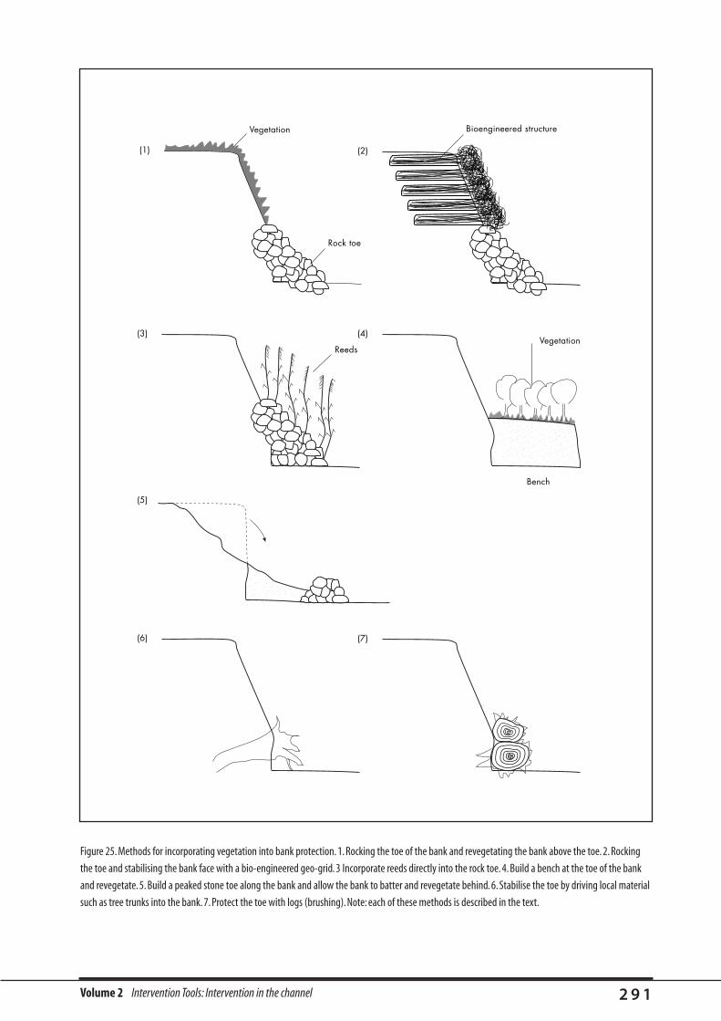
Volume 2 Intervention Tools: Intervention in the channel 2 9 1
Figure 25. Methods for incorporating vegetation into bank protection. 1. Rocking the toe of the bank and revegetating the bank above the toe. 2. Rocking
the toe and stabilising the bank face with a bio-engineered geo-grid. 3 Incorporate reeds directly into the rock toe. 4. Build a bench at the toe of the bank
and revegetate. 5. Build a peaked stone toe along the bank and allow the bank to batter and revegetate behind. 6. Stabilise the toe by driving local material
such as tree trunks into the bank. 7. Protect the toe with logs (brushing). Note: each of these methods is described in the text.
������
(5)
(1)
(3) (4)Vegetation
Bench
Reeds
(6) (7)
Rock toe
(2)
Bioengineered structureVegetation
������
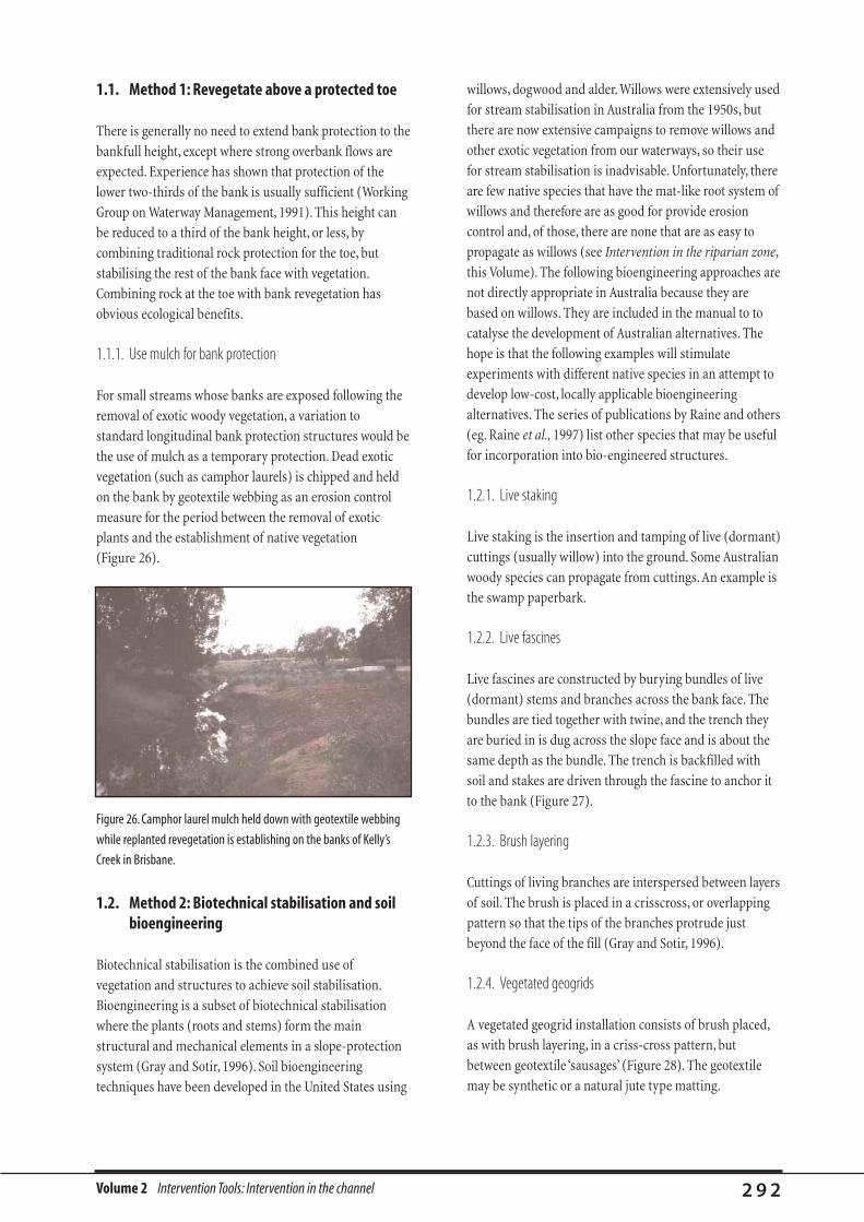
Volume 2 Intervention Tools: Intervention in the channel 2 9 2
1.1. Method 1: Revegetate above a protected toe
There is generally no need to extend bank protection to the
bankfull height, except where strong overbank flows are
expected. Experience has shown that protection of the
lower two-thirds of the bank is usually sufficient (Working
Group on Waterway Management, 1991). This height can
be reduced to a third of the bank height, or less, by
combining traditional rock protection for the toe, but
stabilising the rest of the bank face with vegetation.
Combining rock at the toe with bank revegetation has
obvious ecological benefits.
1.1.1. Use mulch for bank protection
For small streams whose banks are exposed following the
removal of exotic woody vegetation, a variation to
standard longitudinal bank protection structures would be
the use of mulch as a temporary protection. Dead exotic
vegetation (such as camphor laurels) is chipped and held
on the bank by geotextile webbing as an erosion control
measure for the period between the removal of exotic
plants and the establishment of native vegetation
(Figure 26).
1.2. Method 2: Biotechnical stabilisation and soilbioengineering
Biotechnical stabilisation is the combined use of
vegetation and structures to achieve soil stabilisation.
Bioengineering is a subset of biotechnical stabilisation
where the plants (roots and stems) form the main
structural and mechanical elements in a slope-protection
system (Gray and Sotir, 1996). Soil bioengineering
techniques have been developed in the United States using
willows, dogwood and alder. Willows were extensively used
for stream stabilisation in Australia from the 1950s, but
there are now extensive campaigns to remove willows and
other exotic vegetation from our waterways, so their use
for stream stabilisation is inadvisable. Unfortunately, there
are few native species that have the mat-like root system of
willows and therefore are as good for provide erosion
control and, of those, there are none that are as easy to
propagate as willows (see Intervention in the riparian zone,
this Volume). The following bioengineering approaches are
not directly appropriate in Australia because they are
based on willows. They are included in the manual to to
catalyse the development of Australian alternatives. The
hope is that the following examples will stimulate
experiments with different native species in an attempt to
develop low-cost, locally applicable bioengineering
alternatives. The series of publications by Raine and others
(eg. Raine et al., 1997) list other species that may be useful
for incorporation into bio-engineered structures.
1.2.1. Live staking
Live staking is the insertion and tamping of live (dormant)
cuttings (usually willow) into the ground. Some Australian
woody species can propagate from cuttings. An example is
the swamp paperbark.
1.2.2. Live fascines
Live fascines are constructed by burying bundles of live
(dormant) stems and branches across the bank face. The
bundles are tied together with twine, and the trench they
are buried in is dug across the slope face and is about the
same depth as the bundle. The trench is backfilled with
soil and stakes are driven through the fascine to anchor it
to the bank (Figure 27).
1.2.3. Brush layering
Cuttings of living branches are interspersed between layers
of soil. The brush is placed in a crisscross, or overlapping
pattern so that the tips of the branches protrude just
beyond the face of the fill (Gray and Sotir, 1996).
1.2.4. Vegetated geogrids
A vegetated geogrid installation consists of brush placed,
as with brush layering, in a criss-cross pattern, but
between geotextile ‘sausages’ (Figure 28). The geotextile
may be synthetic or a natural jute type matting.
Figure 26. Camphor laurel mulch held down with geotextile webbing
while replanted revegetation is establishing on the banks of Kelly’s
Creek in Brisbane.
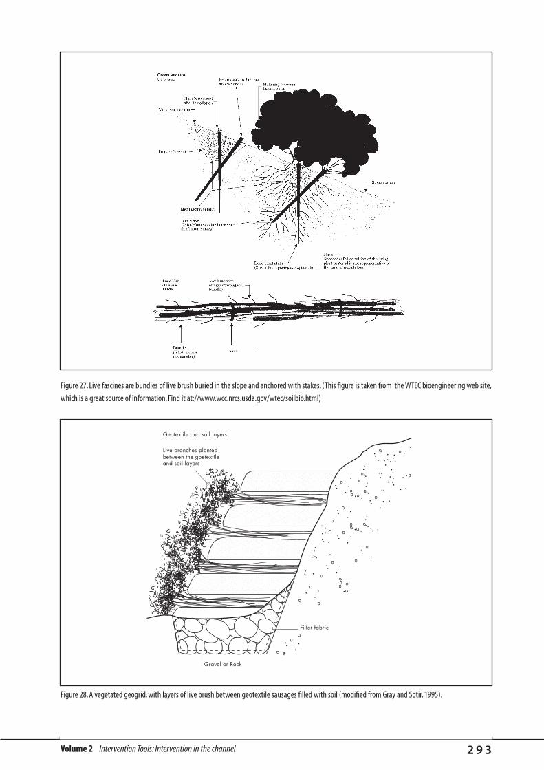
Volume 2 Intervention Tools: Intervention in the channel 2 9 3
Figure 28. A vegetated geogrid, with layers of live brush between geotextile sausages filled with soil (modified from Gray and Sotir, 1995).
Geotextile and soil layers
Live branches plantedbetween the goetextileand soil layers
Filter fabric
Gravel or Rock
����������
����������
����������
����������
Figure 27. Live fascines are bundles of live brush buried in the slope and anchored with stakes. (This figure is taken from the WTEC bioengineering web site,
which is a great source of information. Find it at://www.wcc.nrcs.usda.gov/wtec/soilbio.html)
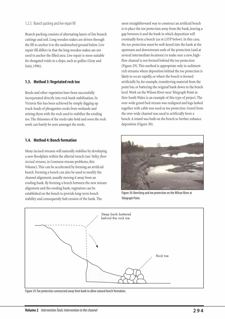
Volume 2 Intervention Tools: Intervention in the channel 2 9 4
1.2.5. Branch packing and live repair fill
Branch packing consists of alternating layers of live branch
cuttings and soil. Long wooden stakes are driven through
the fill to anchor it to the undisturbed ground below. Live
repair fill differs in that the long wooden stakes are not
used to anchor the filled area. Live repair is more suitable
for elongated voids in a slope, such as gullies (Gray and
Sotir, 1996).
1.3. Method 3: Vegetated rock toe
Reeds and other vegetation have been successfully
incorporated directly into rock bank stabilisation. In
Victoria this has been achieved by simply digging up
truck-loads of phragmites reeds from wetlands and
mixing them with the rock used to stabilise the eroding
toe. The rhizomes of the reeds take hold and soon the rock
work can barely be seen amongst the reeds.
1.4. Method 4: Bench formation
Many incised streams will naturally stabilise by developing
a new floodplain within the alluvial trench (see Valley floor
incised streams, in Common stream problems, this
Volume). This can be accelerated by forming an artificial
bench. Forming a bench can also be used to modify the
channel alignment, usually moving it away from an
eroding bank. By forming a bench between the new stream
alignment and the eroding bank, vegetation can be
established on the bench to provide long-term bench
stability and consequently halt erosion of the bank. The
most straightforward way to construct an artificial bench
is to place the toe protection away from the bank, leaving a
gap between it and the bank in which deposition will
eventually form a bench (as in LSTP below). In this case,
the toe protection must be well-keyed into the bank at the
upstream and downstream ends of the protection (and at
several intermediate locations) to make sure a new, high-
flow channel is not formed behind the toe protection
(Figure 29). This method is appropriate only in sediment-
rich streams where deposition behind the toe protection is
likely to occur rapidly, or where the bench is formed
artificially by, for example, transferring material from the
point bar, or battering the original bank down to the bench
level. Work on the Wilson River near Telegraph Point in
New South Wales is an example of this type of project. The
over-wide gravel bed stream was realigned and logs lashed
together with cable was used as toe protection. Gravel from
the over-wide channel was used to artificially form a
bench. A retard was built on the bench to further enhance
deposition (Figure 30).
Figure 29.Toe protection constructed away from bank to allow natural bench formation.
Rock toe
Steep bank batteredbehind the rock toe
������
Figure 30. Benching and toe protection on the Wilson River at
Telegraph Point.

Volume 2 Intervention Tools: Intervention in the channel 2 9 5
The lack of fine material and the fully exposed conditions
on the artificial bench make establishment of vegetation
difficult without careful follow-up work like watering,
weed removal and mulching. The experience of the New
South Wales Department of Land and Water Conservation
is that if the artificial bench is built only slightly (say 10
cm) higher than low-water level, then artificial and natural
regeneration of artificial benches is much quicker and no
follow-up watering is required because seedlings can
quickly reach the moist conditions below the gravel (Allan
Raine, personal communication).
1.5. Method 5: Longitudinal peaked stone toeprotection (LSTP)
LSTP is the placement of a ridge of stone along the toe of
an eroding bank. This is effectively a ‘windrow’ structure
which acts to remove the attack point from the toe of the
bank. The banks behind the toe protection are either
pushed down into the space behind the rock, or left to
naturally batter back. LSTP is one of the most reliable and
economical approaches for stabilising incised streams
(Shields et al., 1995c), and is frequently used to stabilise
incised sand-bed channels (Shields et al., 1998). The in-
stream habitat of incising sand-bed channels is usually
highly degraded, with limited depth variation and cover.
Stone is placed in a ridge, or windrow, several metres out
from the toe of the bank in a triangular or trapezoidal
cross-section with sides at the angle of repose. Crest
elevations are not specified, but the rate of application per
unit length of stream is normally set between 1,500 and
6,000 kg/m (Shields et al., 1995c; Shields et al., 1998).
Observations at the same sites over 18 years have shown
that LSTP applied at 1,500 kg/m to an incised stream
provided reasonable toe protection for a stream with slope
0.001–0.005, and banks 4–5 m high (Shields et al., 1995c).
LSTP is improved by the addition of small groynes (spur
dykes) which act to emulate some of the features of the
woody debris that would have been a natural feature of the
stream before incision (Figure 31) (Shields et al., 1998).
The habitat provided by stone toe protection alone is
inferior to that provided by spur dykes (small groynes)
(Shields et al., 1998). This is largely because of the
uniformity of the flow and depth near toe protection.
Where spur dykes or groynes are used, the hydraulic
diversity and depth variation increases, resulting in
improved habitat features.
The best example of the use of spur dykes to date is from
research in the US, where a site modified with spur dykes
and a control site without spur dykes were monitored over
four years. Results of the study showed that, in the modified
site, median water depth increased, the pool habitat area
increased, fish numbers tripled, median fish size increased,
and the species richness increased (Shields et al., 1995c).
Spur dykes cost more than traditional toe protection alone.
Shields et al. (1998) found that 16% more stone was required
to include spur dykes in longitudinal toe protection.
A successful stream restoration project by Shields et al.
(1998) used the following geometry for spur dykes:
• spur lengths approximately 40% of the channel width;
• crests of the spurs were level;
• crests were 2 m wide and 1 m above the bed (baseflow
depth approx 0.4 m); and
• stone size was from 0.2 to 450 kg with 50–85% of
stones less than 36 kg.
SECTION
PLAN
��������������
������������������������������
���������
Figure 31. Adding spur dykes to longitudinal stone toe protection (from
Shields et al., 1998). Reproduced with permission from the American
Water Resources Association.
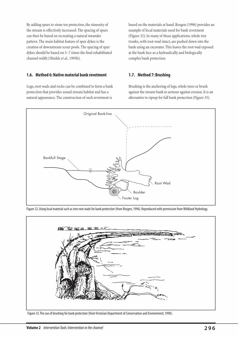
Volume 2 Intervention Tools: Intervention in the channel 2 9 6
By adding spurs to stone toe protection, the sinuosity of
the stream is effectively increased. The spacing of spurs
can then be based on recreating a natural meander
pattern. The main habitat feature of spur dykes is the
creation of downstream scour pools. The spacing of spur
dykes should be based on 5–7 times the final rehabilitated
channel width (Shields et al., 1995b).
1.6. Method 6: Native material bank revetment
Logs, root wads and rocks can be combined to form a bank
protection that provides sound stream habitat and has a
natural appearance. The construction of such revetment is
based on the materials at hand. Rosgen (1996) provides an
example of local materials used for bank revetment
(Figure 32). In many of these applications, whole tree
trunks, with root-wad intact, are pushed down into the
bank using an excavator. This leaves the root wad exposed
at the bank face as a hydraulically and biologically
complex bank protection.
1.7. Method 7: Brushing
Brushing is the anchoring of logs, whole trees or brush
against the stream bank to armour against erosion. It is an
alternative to riprap for full bank protection (Figure 33).
Figure 32. Using local material such as tree root wads for bank protection (from Rosgen, 1996). Reproduced with permission from Wildland Hydrology.
Bankfull Stage
Original Bank-line
Footer Log
Boulder
Root Wad�y
Figure 33.The use of brushing for bank protection (from Victorian Department of Conservation and Environment, 1990).
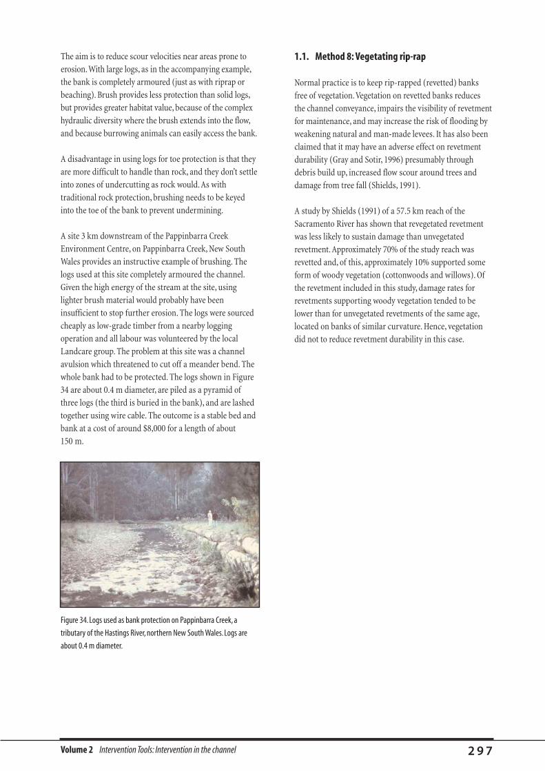
Volume 2 Intervention Tools: Intervention in the channel 2 9 7
The aim is to reduce scour velocities near areas prone to
erosion.With large logs, as in the accompanying example,
the bank is completely armoured (just as with riprap or
beaching). Brush provides less protection than solid logs,
but provides greater habitat value, because of the complex
hydraulic diversity where the brush extends into the flow,
and because burrowing animals can easily access the bank.
A disadvantage in using logs for toe protection is that they
are more difficult to handle than rock, and they don’t settle
into zones of undercutting as rock would. As with
traditional rock protection, brushing needs to be keyed
into the toe of the bank to prevent undermining.
A site 3 km downstream of the Pappinbarra Creek
Environment Centre, on Pappinbarra Creek, New South
Wales provides an instructive example of brushing. The
logs used at this site completely armoured the channel.
Given the high energy of the stream at the site, using
lighter brush material would probably have been
insufficient to stop further erosion. The logs were sourced
cheaply as low-grade timber from a nearby logging
operation and all labour was volunteered by the local
Landcare group. The problem at this site was a channel
avulsion which threatened to cut off a meander bend. The
whole bank had to be protected. The logs shown in Figure
34 are about 0.4 m diameter, are piled as a pyramid of
three logs (the third is buried in the bank), and are lashed
together using wire cable. The outcome is a stable bed and
bank at a cost of around $8,000 for a length of about
150 m.
Figure 34. Logs used as bank protection on Pappinbarra Creek, a
tributary of the Hastings River, northern New South Wales. Logs are
about 0.4 m diameter.
1.1. Method 8: Vegetating rip-rap
Normal practice is to keep rip-rapped (revetted) banks
free of vegetation.Vegetation on revetted banks reduces
the channel conveyance, impairs the visibility of revetment
for maintenance, and may increase the risk of flooding by
weakening natural and man-made levees. It has also been
claimed that it may have an adverse effect on revetment
durability (Gray and Sotir, 1996) presumably through
debris build up, increased flow scour around trees and
damage from tree fall (Shields, 1991).
A study by Shields (1991) of a 57.5 km reach of the
Sacramento River has shown that revegetated revetment
was less likely to sustain damage than unvegetated
revetment. Approximately 70% of the study reach was
revetted and, of this, approximately 10% supported some
form of woody vegetation (cottonwoods and willows). Of
the revetment included in this study, damage rates for
revetments supporting woody vegetation tended to be
lower than for unvegetated revetments of the same age,
located on banks of similar curvature. Hence, vegetation
did not to reduce revetment durability in this case.
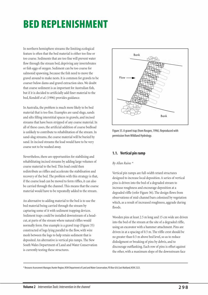
Volume 2 Intervention Tools: Intervention in the channel 2 9 8
In northern hemisphere streams the limiting ecological
feature is often that the bed material is either too fine or
too coarse. Sediments that are too fine will prevent water
flow through the stream bed, depriving any invertebrates
or fish eggs of oxygen. Sediment can be too coarse for
salmonid spawning, because the fish need to move the
gravel around to make nests. It is common for gravels to be
coarser below dams and gravel extraction sites. We doubt
that coarse sediment is as important for Australian fish,
but if it is decided to artificially add finer material to the
bed, Kondolf et al. (1996) provides guidance.
In Australia, the problem is much more likely to be bed
material that is too fine. Examples are sand slugs, sands
and silts filling interstitial spaces in gravels, and incised
streams that have been stripped of any coarse material. In
all of these cases, the artificial addition of coarse bedload
is unlikely to contribute to rehabilitation of the stream. In
sand-slug streams, the coarse material will be buried by
sand. In incised streams the load would have to be very
coarse not to be washed away.
Nevertheless, there are opportunities for stabilising and
rehabilitating incised streams by adding large volumes of
coarse material to the bed. This load could then
redistribute as riffles and accelerate the stabilisation and
recovery of the bed. The problem with this strategy is that,
if the coarse load can be moved to form riffles, it can also
be carried through the channel. This means that the coarse
material would have to be repeatedly added to the stream.
An alternative to adding material to the bed is to use the
bed material being carried through the stream by
capturing some of it with sediment trapping devices.
Sediment traps could be installed downstream of a head-
cut, at parts of the stream where natural riffles would
normally form. One example is a gravel trap (Figure 35)
constructed of logs lying parallel to the flow, with wire
mesh between the logs to help retain sediment that is
deposited. An alternative is vertical pin ramps. The New
South Wales Department of Land and Water Conservation
is currently testing these structures.
1.1. Vertical pin ramp
By Allan Raine *
Vertical pin ramps are full-width retard structures
designed to increase local deposition. A series of vertical
pins is driven into the bed of a degraded stream to
increase roughness and encourage deposition at a
degraded riffle (refer Figure 36). The design flows from
observations of mid-channel bars colonised by vegetation
which, as a result of increased roughness, aggrade during
floods.
Wooden pins at least 2.5 m long and 15 cm wide are driven
into the bed of the stream at the site of a degraded riffle,
using an excavator with a hammer attachment. Pins are
driven in at a spacing of 0.5 m. The riffle crest should be
no greater than 0.5 m above bed level, so as to reduce
dislodgment or breaking of pins by debris, and to
discourage outflanking. Each row of pins is offset against
the other, with a maximum slope of the downstream face
BED REPLENISHMENT
Bank
Flow
Bank
����������
������������
Figure 35. A gravel trap (from Rosgen, 1996). Reproduced with
permission from Wildland Hydrology.
* Resource Assessment Manager, Hunter Region, NSW Department of Land and Water Conservation, PO Box 424, East Maitland, NSW 2323.
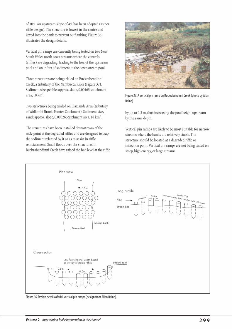
Volume 2 Intervention Tools: Intervention in the channel 2 9 9
of 10:1. An upstream slope of 4:1 has been adopted (as per
riffle design). The structure is lowest in the centre and
keyed into the bank to prevent outflanking. Figure 36
illustrates the design details.
Vertical pin ramps are currently being tested on two New
South Wales north coast streams where the controls
(riffles) are degrading, leading to the loss of the upstream
pool and an influx of sediment to the downstream pool.
Three structures are being trialed on Buckrabendinni
Creek, a tributary of the Nambucca River (Figure 37).
Sediment size, pebble; approx. slope, 0.00165; catchment
area, 10 km2.
Two structures being trialed on Blaxlands Arm (tributary
of Wollombi Brook, Hunter Catchment). Sediment size,
sand; approx. slope, 0.00526; catchment area, 18 km2.
The structures have been installed downstream of the
nick-point at the degraded riffles and are designed to trap
the sediment released by it so as to assist in riffle
reinstatement. Small floods over the structures in
Buckrabendinni Creek have raised the bed level at the riffle
by up to 0.3 m, thus increasing the pool height upstream
by the same depth.
Vertical pin ramps are likely to be most suitable for narrow
streams where the banks are relatively stable. The
structure should be located at a degraded riffle or
inflection point.Vertical pin ramps are not being tested on
steep, high energy, or large streams.
Figure 36. Design details of trial vertical pin ramps (design from Allan Raine).
Flow
Low flow channel width basedon survey of stable riffles
0.5m
0.5m0.5m
Stream Bed
Stream Bed
Long profile
Cross-section
Plan view
Stream Bank
Stream Bank
Flow0.5m
grade 4:1(minimum: may be flatter based on stable riffle survey)
grade 10:1
Figure 37. A vertical pin ramp on Buckrabendinni Creek (photo by Allan
Raine).

Volume 2 Intervention Tools: Intervention in the channel 3 0 0
REINSTATING CUT-OFF MEANDERS
1. Introduction
Between the 1870s and 1970s numerous Australian
streams were artificially straightened. The aim of these
works was to increase the flow conveyance of the channel
in order to improve the drainage and reduce the frequency
and duration of overbank flooding. The consequences of
this type of ‘improvement’ have been documented in
Australia (Reinfelds et al., 1995) and in many studies
around the world (Brookes, 1988). They include deepening
and widening of the channel, and major decline in
ecological function.
In order to rehabilitate straightened channels, streams are
being returned to their original courses (Keller, 1995).
Meanders can be rehabilitated in two ways: by the
reintroduction of meanders that were previously cut off;
and by the construction of new bends in undisturbed
floodplain sediment (Brookes, 1996). There are several
procedures for the design of meanders, as discussed in the
Natural channel design, this Volume. Below is a description
of the reinstatement of cut-off meander bends on the
Latrobe River in Victoria—probably the largest exercise of
its kind in Australia.
Meanderreinstatement onthe Latrobe RiverThe lower Latrobe River (Gippsland,Victoria) is a clay and sand
bed stream, approximately 240 km long, with a catchment of
5,200 km2 and an average width of about 30 m. Sixty-six
artificial meander cut-offs have been made in the Latrobe since
the 1870s, with most occurring in the 1960s (Figure 38).The
length of stream was reduced by 25%, and sinuosity decreased
from 2.12 to 1.59 (Reinfelds et al., 1995).The cut-offs where
installed to improve the hydraulic capacity of the river and get
floodwaters away more quickly.They were excavated as
depressions lower than the bankfull conditions, so high flows
would preferentially flow through the cut-off before
overtopping the bank. Unfortunately, the cut-offs quickly
downcut and eroded to become the main channel and the
original meanders became backwaters.
The meanders were reinstated:
• to reduce accelerated bank erosion on the bends
downstream of the cut-offs; and
• to restore a high-quality riparian zone along long reaches of
the river by incorporating the isolated islands that were
created by the cut-offs.These islands retained their original
riparian vegetation.
The Lake Wellington Rivers Authority reinstated six of the
original meanders while maintaining the original design flow
conveyance conditions of the cut-offs.The openings to the
artificial cut-offs were blocked with a rock weir up to the
design height of the original chute. A narrow pilot channel was
excavated in the natural channel that allowed water to flow
through the original course. If the meanders had been partly or
completely filled in, the whole meander would have been
excavated to a bed slope that connects the upstream and
downstream bed levels.
Figure 38. Aerial view of a meander cut-off on the Latrobe River.
Crown (State of Victoria) Copyright. Reproduced with permission of
Land Victoria, Department of Natural Resources and Environment.

cost of the Latrobe River meander reinstatement work was
providing machinery access to isolated sites. To get the
machinery and rock to the sites was a major exercise, with
roads constructed at many sites. Total reinstatement costs
were about $25,000 for each cut-off.
Volume 2 Intervention Tools: Intervention in the channel 3 0 1
The meander bend reinstatement on the Latrobe River was based
on the original cut-off plans for the stream.The eroded cut-offs
each had a bench which represented the original excavation
depth of the cut-offs, so it was easy to identify the design height
for the weir.Rock material was brought in and dumped in the cut-
offs up to the original depth of excavation.The rock material was
won from a local quarry operated by the Lake Wellington Rivers
Authority.Because of the type of rock and machinery available,
rock sizes could not be controlled easily, so what was used was
larger than required for the hydraulic conditions, but cheaper than
bringing in breaking and sorting equipment.
Following the meander reinstatement, Lake Wellington Rivers
Authority began revegetation.The authority is selectively
removing willows from the river banks and hand-planting
swamp paperbarks (Melaleuca ericafolia) by boat along the
stream banks.
The pilot cuts in the original channels developed rapidly (within 2
years). No formal evaluation of the effect of the reinstatement on
bank erosion was completed, although the stream managers are
convinced that the erosion rate declined following the
reinstatement. (Note that this is an example of a Plastic Medal
evaluation design! See Evaluation section, this Volume or Step
10 in Volume 1.)
A more effective evaluation would have been to measure the
proportions of the discharge flowing down the original channel
and the cut-off channel at low and high flows. A comparison of
such measurements from before and after the reinstatement of
the meanders would allow assessment of how much the work
had increased the flow through the original channel.
Several bends on the Latrobe river were not suitable for
reinstatement because the new channel had deepened up
and downstream of the cut-off, to the extent that the old
channel was perched above the level of the present
channel. For this reason, the reinstatement program was
restricted to the lower reaches of the river where the river
did not incise following the cut-offs.
The feasibility of meander bend reinstatement will depend
on the extent of degradation and the availability of the
original meander bends. Where the bends have been
completely filled, or the land ownership makes the
purchase of the bends prohibitive, it is probably more cost
effective to rehabilitate a less-degraded part of the stream.
The reinstatement of meanders on the nearby Moe River
(Gippsland,Victoria) would, for example, be prohibitively
expensive. Following stream straightening, the river has
incised over 1.5 m and the meander bends have been filled
(Figure 39).
Another important point in determining where to reinstate
meanders is the establishment costs of the work. The major
Figure 39.Twenty kilometres of the Moe River in Victoria has been
straightened and original meander bends have been backfilled,
making reinstatement of meander cut-offs uneconomical.
2. Where is re-meandering inappropriate?

Volume 2 Intervention Tools: Intervention in the channel 3 0 2
Re-meandering will have two secondary effects:
• there will be a pulse of sediment from the newly
meandered channel; and
• the flood stage will rise for the same discharge.
At a minimum, the sediment filling the former meander
channel will be remobilised, leading to an increase in
turbidity downstream. Also, if a new meandering channel
has been cut it will certainly erode to some extent as it
stabilises.
Re-meandering projects are common in northern Europe,
particularly Denmark (Brookes, 1996), but there is a
fundamental difference between the situation there and
that in most of Australia. The primary objective in many
northern European schemes (especially in Denmark) is to
raise the watertable in the adjacent floodplain and increase
the frequency of overbank flows, in order to regenerate
degraded riparian wetland ecosystems (Neilsen, 1996),
and to promote sports fisheries. In Australia, on the other
hand, remeandering is usually undertaken with the
specific aim of improving the instream habitat while
generating the minimum increase in flood risk.
There are several ways in which it is possible to estimate
the impact of re-meandering on the flood characteristics
of a stream, including using How changing the channel can
affect flooding, in Natural channel design, this Volume.
Alternatively we can consider what happens when we
channelise a stream, and assume that re-meandering
should have the opposite effect. For example, Shankman
and Pugh (1992) examined the changes resulting from the
channelisation of the Obion River in Tennessee. If we think
in terms of a reversal of the effects of channelisation, we
might predict the following effects of re-meandering.
• Decreased peak discharge downstream of the scheme,
as the increased flow resistance prevents the
floodwaters from converging so quickly at a
downstream point.
• The increased resistance is a result of a rougher channel
perimeter, reduced uniformity in cross-section,
decreased hydraulic radius and decreased slope.
• The frequency of flooding will decrease downstream of
the reintroduced meanders, but the duration of those
floods may increase as the flow in the channel is not as
efficiently removed from the site of the flooding.
• The importance of position in the stream network was
stressed by Shankman and Pugh (1992), whose work
was conducted on a stretch of the Obion immediately
upstream of a confluence with the lower Mississippi
River. When the Mississippi was at a high stage, it
produced a backwater that extended some distance up
the Obion, and controlled flooding in its lower reaches.
Any channelisation or re-meandering work that might
have been carried out in that reach would have had no
effect on the flood characteristics, as discussed in How
changing the channel can affect flooding, in Natural
channel design, this Volume.
Of course re-meandering will not immediately reinstate the
pre-channelisation flood regime. It is likely that the
channelised river is now larger than its predecessor, and the
channel would almost certainly have been cleared of LWD.
To conclude, the Latrobe River example demonstrates that
remeandering can be feasible, and probably effective.
However, in channels that have deepened and enlarged,
and where the old cut-off channels have filled with
sediment, re-meandering will be less successful.
3. Secondary effects of re-meandering

Volume 2 Intervention Tools: Intervention in the channel 3 0 3
FISH COVERCover refers to instream and overhead features that protect
fish from high current velocities, provide concealment for
both predators and prey, and maintain water temperature
by controlling illumination of the water (Swales and
O’Hara, 1980; Wesche, 1985; Gore and Shields, 1995). Cover
requirements (as with other habitat features) are species
and life-stage specific for aquatic organisms. The cover
requirements for salmonid fish have been well researched.
One study by Elser (1968) compared an unaltered stream
section with an altered section with 80% less cover. The
results of the study showed 78% more trout in the
unaltered reach. Cover is also a key habitat element for
Australian native fish. The specific requirements of some
fish are known: trout cod and freshwater blackfish, for
example, prefer hollow logs for spawning (Koehn and
O’Connor, 1990). Recent surveys of platypus habitat have
found that the presence of these animals is strongly
associated with undercut river banks. As a general rule, the
addition of cover will improve the in-stream environment
for aquatic biota, particularly if LWD is used to create
cover. The following illustrations (Figures 40 and 41) are
some examples of artificial cover taken from the
international literature—they may help to inspire local
adaptations that can be incorporated into other in-stream
works, or indeed can be installed on their own.
Figure 40. Floating log and tree cover used in North America as fish
shelter (from Rosgen, 1996). Australian riparian vegetation species
often do not float, so an adaptation of this type of cover might be the
introduction of large woody debris to the stream and anchoring it into
place. Reproduced with permission from Wildland Hydrology.
Figure 41.This snag (perfect habitat!) was reintroduced to Ryans Creek
in Victoria.The cost of relocating the debris from the floodplain and
securing it in the stream was about $500.
Cross section
Plan view
Bank
Bank
Flow
Bank

Volume 2 Intervention Tools: Intervention in the channel 3 0 4
The addition of boulders to a stream flow creates hydraulic
diversity. As flow accelerates around boulders, scour pools
are created and downstream bars are formed. The
boulders create cover and substrate for
macroinvertebrates, and the turbulence generated aerates
the water. Boulders are normally placed mid channel,
where they produce localised bed scour and deposition.
When placed near the bank they may cause localised bank
erosion. An example of the use of boulders to create
improved instream habitat is Ryans Creek (a tributary of
the Broken River in Victoria). The rehabilitation strategy
for a section of shallow, fast-flowing water (glide), was to
place boulders downstream of a log sill, use artificial riffles
to add water depth, introduce large woody debris (one
large snag introduced) and narrow the low-flow channel
using low deflectors (Figure 42).
Boulders are a low-cost alternative stream rehabilitation
structure. For example, the cost of extensive use of
boulders (2,000 ´ 0.5 m3 boulders) in the rehabilitation of
the Snowy River is estimated at around $30 per boulder
(installed) (Stewardson et al., 1997). There are large
economies of scale with this project, and establishment
costs are not included.
BOULDERS
Figure 42. Boulders used to create habitat in Ryans Creek, a tributary of
the Broken River, in Victoria.
The overall consideration when installing boulders is to
ensure that they add to the channel as much hydraulic
disturbance as possible, so as to encourage scour and bar
formation for improved in-stream habitat. This is
generally achieved by selecting large angular boulders
which are placed in the highest-velocity zone of the stream
and orientated to create the greatest hydraulic disturbance.
Quarried boulders are the best material to use, because
their sharp edges enhance turbulence and create the
greatest hydraulic flow diversity. Wesche (1985) suggests
using hard rock (say basalt) in preference to soft rock (say
sandstone), but this choice will be determined largely by
the materials available. Almost anything could be used to
create similar hydraulic disturbance to boulders, but an
obvious consideration is the aesthetic appeal, so use
natural products wherever possible.
1.1. Sizing boulders
• If the ratio of boulder to bed material size is less than
approximately 20:1 the boulders may ‘glide’ over the
bed material in high flows (Conrick and Ribi, 1996).
• Rocks could be sized on the basis of tractive force
equations, but realistically, the size needed to create
suitable habitat features is usually much larger than the
critical size for transport. Wesche (1985) suggests a
diameter between 0.6 m and 1.5 m.
• Barton and Cron (1979) (in Shields, 1984) recommend
that boulders should be no larger in their greatest
dimension than one fifth of the normal-flow channel
width. This recommendation is presumably to avoid
over-constricting the flow in the channel and thereby
causing bank erosion.
1.2. Placement of boulders
• Wesche (1985) recommends embedding boulders into
the stream bed, but if they are large compared with the
minimum size required to resist tractive stress
movement, there is little value in further anchoring
them.
• Boulders are effective because they create hydraulic
disturbance, so they should be positioned to maximise
1. Installing boulders

Volume 2 Intervention Tools: Intervention in the channel 3 0 5
that disturbance by orientating their longest dimension
at right angles to the flow, as in Figure 42, and by
placing them near the centre of the stream or fastest-
flowing area (Shields, 1984).
• To ensure boulders have the greatest hydraulic impact
they should not be placed in the downstream zone of
influence (wake) of upstream boulders.
• Boulders can cause local bank scour, so do not place
them near banks susceptible to erosion (Wesche, 1985).
• Shields (1984) suggests that boulders should project
slightly above the water surface at normal flow. This is
presumably for the benefit of non-aquatic wildlife such
as birds.
• Boulders are best applied to shallow, high to mid-
gradient streams. The main mode of failure of boulders
is that they may be buried in low gradient sand-bed
streams (Shields, 1984). In these stream types they
tend to ‘drill’ themselves into the bed as sand is scoured
from under them.
• In slower, deeper streams the effect of the boulder is
drowned out.
• Boulders create only minor increases in channel
roughness during bankfull flow conditions.
1.3. Spacing boulders
There are no Australian data on which to recommend the
spacing of boulders. Shields (1984) presents the
recommendations of two studies:
• one rock per 27 m2 (Barton and Cron, 1979); and
• one 2 m diameter boulder approximately every 70 m2
provided superior habitat to one boulder per 46 m2
(Kanaly, 1975).
However, the optimum spacing of boulders is dependent
on the habitat requirements of particular species, and the
presence of other habitat features. One important finding
of Kanaly (1975), as reported by Shields (1984), was that
the pattern of boulder placement had no effect on fish
density. Suggestions for suitable boulder placements are
shown in Figure 43.
Figure 43. Patterns for boulder placements (from Wesche, 1985).
Reproduced with permission from Butterworth Publishing.
Boulder(embedded)
Scour Pool
Boulder Placements
Flow
Upstream "V"
Downstream "V"
Stab
le B
ank
����yyyy����yyyy��yy
��yy
��yy��yy
�y��yy��yy
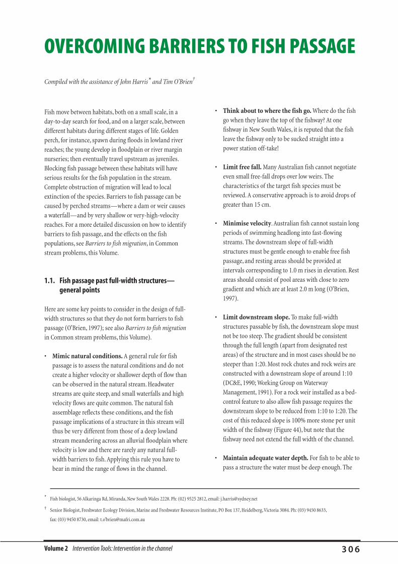
Volume 2 Intervention Tools: Intervention in the channel 3 0 6
Compiled with the assistance of John Harris* and Tim O’Brien†
OVERCOMING BARRIERS TO FISH PASSAGE
Fish move between habitats, both on a small scale, in a
day-to-day search for food, and on a larger scale, between
different habitats during different stages of life. Golden
perch, for instance, spawn during floods in lowland river
reaches; the young develop in floodplain or river margin
nurseries; then eventually travel upstream as juveniles.
Blocking fish passage between these habitats will have
serious results for the fish population in the stream.
Complete obstruction of migration will lead to local
extinction of the species. Barriers to fish passage can be
caused by perched streams—where a dam or weir causes
a waterfall—and by very shallow or very-high-velocity
reaches. For a more detailed discussion on how to identify
barriers to fish passage, and the effects on the fish
populations, see Barriers to fish migration, in Common
stream problems, this Volume.
1.1. Fish passage past full-width structures—general points
Here are some key points to consider in the design of full-
width structures so that they do not form barriers to fish
passage (O’Brien, 1997); see also Barriers to fish migration
in Common stream problems, this Volume).
• Mimic natural conditions. A general rule for fish
passage is to assess the natural conditions and do not
create a higher velocity or shallower depth of flow than
can be observed in the natural stream. Headwater
streams are quite steep, and small waterfalls and high
velocity flows are quite common. The natural fish
assemblage reflects these conditions, and the fish
passage implications of a structure in this stream will
thus be very different from those of a deep lowland
stream meandering across an alluvial floodplain where
velocity is low and there are rarely any natural full-
width barriers to fish. Applying this rule you have to
bear in mind the range of flows in the channel.
• Think about to where the fish go. Where do the fish
go when they leave the top of the fishway? At one
fishway in New South Wales, it is reputed that the fish
leave the fishway only to be sucked straight into a
power station off-take!
• Limit free fall. Many Australian fish cannot negotiate
even small free-fall drops over low weirs. The
characteristics of the target fish species must be
reviewed. A conservative approach is to avoid drops of
greater than 15 cm.
• Minimise velocity. Australian fish cannot sustain long
periods of swimming headlong into fast-flowing
streams. The downstream slope of full-width
structures must be gentle enough to enable free fish
passage, and resting areas should be provided at
intervals corresponding to 1.0 m rises in elevation. Rest
areas should consist of pool areas with close to zero
gradient and which are at least 2.0 m long (O’Brien,
1997).
• Limit downstream slope. To make full-width
structures passable by fish, the downstream slope must
not be too steep. The gradient should be consistent
through the full length (apart from designated rest
areas) of the structure and in most cases should be no
steeper than 1:20. Most rock chutes and rock weirs are
constructed with a downstream slope of around 1:10
(DC&E, 1990; Working Group on Waterway
Management, 1991). For a rock weir installed as a bed-
control feature to also allow fish passage requires the
downstream slope to be reduced from 1:10 to 1:20. The
cost of this reduced slope is 100% more stone per unit
width of the fishway (Figure 44), but note that the
fishway need not extend the full width of the channel.
• Maintain adequate water depth. For fish to be able to
pass a structure the water must be deep enough. The
* Fish biologist, 56 Alkaringa Rd, Miranda, New South Wales 2228. Ph: (02) 9525 2812, email: [email protected]
† Senior Biologist, Freshwater Ecology Division, Marine and Freshwater Resources Institute, PO Box 137, Heidelberg,Victoria 3084. Ph: (03) 9450 8633,
fax: (03) 9450 8730, email: t.o’[email protected]

Volume 2 Intervention Tools: Intervention in the channel 3 0 7
depth of water required will depend on the fish
assemblage present but, as a general rule, coastal
streams should be at least 15 cm deep during the
minimum design flow period, and inland streams may
need to be deeper because of the larger species present
in these river systems. The minimum design flow that
should be used for designing fishways is unclear, but
one suggestion is that fish should have free passage
past channel obstructions for 95% of the time that the
stream is actually flowing (J.Harris, personal
communication).
There are several ways to maintain a minimum depth
of flow over full-width structures. For the construction
of riffles (rock weirs) Newbury and Gaboury (1993)
recommend the structure be V-shaped to concentrate
low flow at its centre. The slope of the crest into the V is
only slight: Newbury and Gaboury (1993) use a drop of
0.1 m from the banks to the centre of the channel for
streams 10–15 m wide.
The double arch sill in Figure 45 incorporates a similar
concept, with a lower gradient, central chute for fish
passage at low flow. An alternative design is the use of a
zigzag fish ladder up the face of the grade control
structure to reduce the effective slope of the low-flow
water surface (Figure 46). For this design, rock should
be oversized to resist movement in the high shear-
stress zone down the face of the structure.
1.2. Fish passage over larger structures—rock-ramp fishways
There are many thousands of barriers to fish passage
around Australia. The average cost to build concrete
fishways, such as the vertical-slot design, for each of these
structures would be measured in hundreds of thousands
of dollars (Mallen-Cooper and Harris, 1990). Clearly, this is
a daunting task and funding even a long-term program to
restore fish passage will be difficult. If you need a large
engineered structure like this, then seek professional
advice! Most managers need a cheaper alternative, and the
type of fishway that is most likely to be appropriate is the
rock-ramp fishway. This is particularly suitable for the
numerous barriers that are less than 1 m or so in height.
Rock-ramp fishways are being tested by New South Wales
Fisheries, the New South Wales Department of Land and
Water Conservation, the Cooperative Research Centre for
Rock used for weir
+ 100%
Additional rock required for fish passage
1:4
1:201:10
Figure 44.The additional volume of rock required when you halve the slope of a rock chute to provide fish passage.
Figure 45. A mangfall sill with central fishway (photo by John Harris).
Figure 46. A zigzag fishway, with transverse ridges of rock that
effectively reduce the slope of the fishway (photo by John Harris).
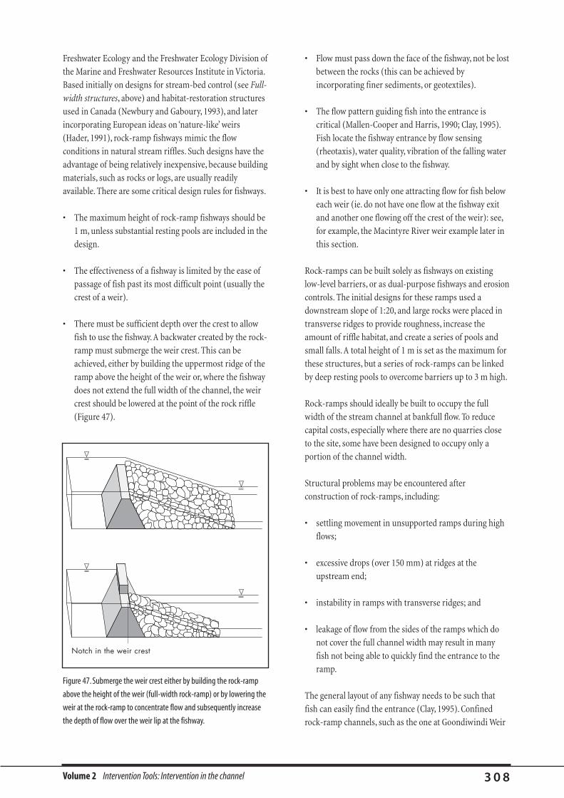
Volume 2 Intervention Tools: Intervention in the channel 3 0 8
Freshwater Ecology and the Freshwater Ecology Division of
the Marine and Freshwater Resources Institute in Victoria.
Based initially on designs for stream-bed control (see Full-
width structures, above) and habitat-restoration structures
used in Canada (Newbury and Gaboury, 1993), and later
incorporating European ideas on ‘nature-like’ weirs
(Hader, 1991), rock-ramp fishways mimic the flow
conditions in natural stream riffles. Such designs have the
advantage of being relatively inexpensive, because building
materials, such as rocks or logs, are usually readily
available. There are some critical design rules for fishways.
• The maximum height of rock-ramp fishways should be
1 m, unless substantial resting pools are included in the
design.
• The effectiveness of a fishway is limited by the ease of
passage of fish past its most difficult point (usually the
crest of a weir).
• There must be sufficient depth over the crest to allow
fish to use the fishway. A backwater created by the rock-
ramp must submerge the weir crest. This can be
achieved, either by building the uppermost ridge of the
ramp above the height of the weir or, where the fishway
does not extend the full width of the channel, the weir
crest should be lowered at the point of the rock riffle
(Figure 47).
• Flow must pass down the face of the fishway, not be lost
between the rocks (this can be achieved by
incorporating finer sediments, or geotextiles).
• The flow pattern guiding fish into the entrance is
critical (Mallen-Cooper and Harris, 1990; Clay, 1995).
Fish locate the fishway entrance by flow sensing
(rheotaxis), water quality, vibration of the falling water
and by sight when close to the fishway.
• It is best to have only one attracting flow for fish below
each weir (ie. do not have one flow at the fishway exit
and another one flowing off the crest of the weir): see,
for example, the Macintyre River weir example later in
this section.
Rock-ramps can be built solely as fishways on existing
low-level barriers, or as dual-purpose fishways and erosion
controls. The initial designs for these ramps used a
downstream slope of 1:20, and large rocks were placed in
transverse ridges to provide roughness, increase the
amount of riffle habitat, and create a series of pools and
small falls. A total height of 1 m is set as the maximum for
these structures, but a series of rock-ramps can be linked
by deep resting pools to overcome barriers up to 3 m high.
Rock-ramps should ideally be built to occupy the full
width of the stream channel at bankfull flow. To reduce
capital costs, especially where there are no quarries close
to the site, some have been designed to occupy only a
portion of the channel width.
Structural problems may be encountered after
construction of rock-ramps, including:
• settling movement in unsupported ramps during high
flows;
• excessive drops (over 150 mm) at ridges at the
upstream end;
• instability in ramps with transverse ridges; and
• leakage of flow from the sides of the ramps which do
not cover the full channel width may result in many
fish not being able to quickly find the entrance to the
ramp.
The general layout of any fishway needs to be such that
fish can easily find the entrance (Clay, 1995). Confined
rock-ramp channels, such as the one at Goondiwindi Weir
Notch in the weir crest
Figure 47. Submerge the weir crest either by building the rock-ramp
above the height of the weir (full-width rock-ramp) or by lowering the
weir at the rock-ramp to concentrate flow and subsequently increase
the depth of flow over the weir lip at the fishway.
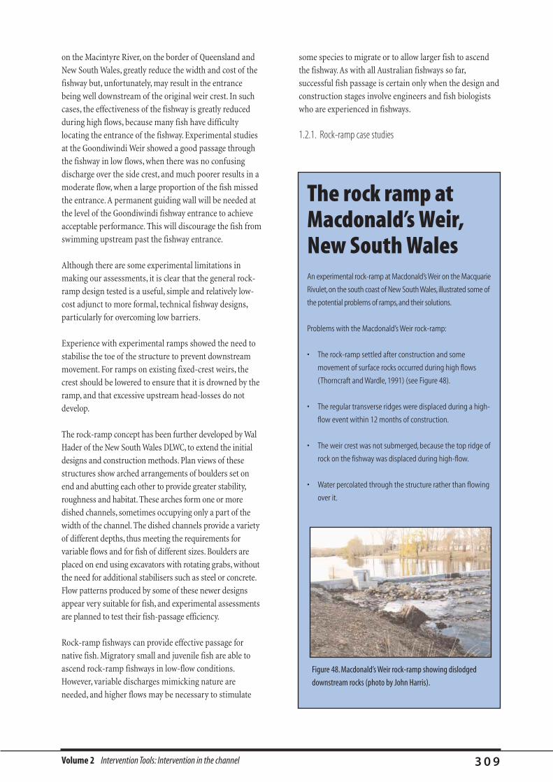
Volume 2 Intervention Tools: Intervention in the channel 3 0 9
on the Macintyre River, on the border of Queensland and
New South Wales, greatly reduce the width and cost of the
fishway but, unfortunately, may result in the entrance
being well downstream of the original weir crest. In such
cases, the effectiveness of the fishway is greatly reduced
during high flows, because many fish have difficulty
locating the entrance of the fishway. Experimental studies
at the Goondiwindi Weir showed a good passage through
the fishway in low flows, when there was no confusing
discharge over the side crest, and much poorer results in a
moderate flow, when a large proportion of the fish missed
the entrance. A permanent guiding wall will be needed at
the level of the Goondiwindi fishway entrance to achieve
acceptable performance. This will discourage the fish from
swimming upstream past the fishway entrance.
Although there are some experimental limitations in
making our assessments, it is clear that the general rock-
ramp design tested is a useful, simple and relatively low-
cost adjunct to more formal, technical fishway designs,
particularly for overcoming low barriers.
Experience with experimental ramps showed the need to
stabilise the toe of the structure to prevent downstream
movement. For ramps on existing fixed-crest weirs, the
crest should be lowered to ensure that it is drowned by the
ramp, and that excessive upstream head-losses do not
develop.
The rock-ramp concept has been further developed by Wal
Hader of the New South Wales DLWC, to extend the initial
designs and construction methods. Plan views of these
structures show arched arrangements of boulders set on
end and abutting each other to provide greater stability,
roughness and habitat. These arches form one or more
dished channels, sometimes occupying only a part of the
width of the channel. The dished channels provide a variety
of different depths, thus meeting the requirements for
variable flows and for fish of different sizes. Boulders are
placed on end using excavators with rotating grabs, without
the need for additional stabilisers such as steel or concrete.
Flow patterns produced by some of these newer designs
appear very suitable for fish, and experimental assessments
are planned to test their fish-passage efficiency.
Rock-ramp fishways can provide effective passage for
native fish. Migratory small and juvenile fish are able to
ascend rock-ramp fishways in low-flow conditions.
However, variable discharges mimicking nature are
needed, and higher flows may be necessary to stimulate
some species to migrate or to allow larger fish to ascend
the fishway. As with all Australian fishways so far,
successful fish passage is certain only when the design and
construction stages involve engineers and fish biologists
who are experienced in fishways.
1.2.1. Rock-ramp case studies
The rock ramp atMacdonald’s Weir,New South WalesAn experimental rock-ramp at Macdonald’s Weir on the Macquarie
Rivulet,on the south coast of New South Wales, illustrated some of
the potential problems of ramps,and their solutions.
Problems with the Macdonald’s Weir rock-ramp:
• The rock-ramp settled after construction and some
movement of surface rocks occurred during high flows
(Thorncraft and Wardle, 1991) (see Figure 48).
• The regular transverse ridges were displaced during a high-
flow event within 12 months of construction.
• The weir crest was not submerged, because the top ridge of
rock on the fishway was displaced during high-flow.
• Water percolated through the structure rather than flowing
over it.
Figure 48. Macdonald’s Weir rock-ramp showing dislodged
downstream rocks (photo by John Harris).
Volume 2 Intervention Tools: Intervention in the channel 3 1 0
Solutions:
• Substantial reconstruction was required to restore
the fishway’s function. The rock-ramp was
repaired as follows.
• The problems with settling of the rock and
displacement of the top ridge of rock were solved
by placing larger rocks (diameter > 1 m) on the
top ridge to submerge the weir crest.
• A geotech filter fabric was used to limit
percolation of flow through the rock-ramp.
• Experience with instability of the Macdonald’s
Weirs rock-ramp showed that it would have been
better to lower the old weir crest during
construction, so that subsequent rock settling
would not affect the fishway exit.
• If the lowering of an existing weir is not possible,
only large rocks should be used on the surface of
the ramp. Most importantly, the toe of the ramp
should be stabilised to prevent downstream
movement of the toe rocks and settling of the rest
of the material. This can be done with large
embedded rocks, sheet-pile, timber or railway-line
driven into the river bed.
small pools. Bank stability is enhanced with rock or
timberwork and plantings of local species. European
experience suggests that by-pass channels have performed
effectively, and in some regions technical fishways are being
dismantled and replaced by bypasses.Australian water
agencies need to experiment with this technology to
determine its value for solving local fish-passage problems.
The bypass rock-ramp at LowerBarwon RiverbarrageAn off-stream rock fishway was constructed around the Lower
Barwon River (Victoria) barrage (see Figure 49).The barrage is a
sheet pile weir approximately 0.75 m high for impounding
water and acting as a tidal barrier.The construction of the rock-
ramp fishway coincided with the refurbishment of the weir.
The rock weir extends across the width of the channel and has
a slope of 1:16.The weir was lowered at the entry point of the
rock-ramp by cutting a 2.5 m wide (fishway width) and 100
mm deep slot through one side of the weir.The rock ramp was
lined with geotextile material, and the final layer of rocks
placed on the ramp. Large rocks were placed on the rock ramp
under the direction of a fish biologist while the water was
being released down the ramp.This allowed the selection and
adjustment of rocks so that flow patterns allowed fish passage
by providing low enough velocities, sufficient depth and
resting sites up the ramp.The materials for this project were: 24
m3 of quarried rock 200–700 mm diameter; 6 m3 of quarry
scalpings; and 8 x 3.6 m polyweave-F geotextile filter fabric.
Two days of front-end loader time plus labour were needed,
and the total cost of the project was approximately $10,000.
The fishway has been tested by two major floods with no
significant damage. Based on this and the shallow channel and
wide floodplain at the site, the fishway is not expected to be
damaged by floods.
Electro-fishing of areas above, below and within the fishway,
showed that the completed rock-ramp posed only a minimal
impediment to fish movement. Catches from these areas were
similar in terms of both relative abundance and fish size range,
and fish were relatively evenly distributed throughout the
fishway itself (O'Brien, 1997).
1.2.2. Fish bypass channels
Fish bypass channels are another potential fishway design
for Australia. In Europe, bypass channels are being applied
to provide successful passage for a wide range of fish
species and sizes past low dams, weirs and other barriers
up to 8 m in height. They are low gradient earthen or rocky
channels that mimic the structure of natural streams, and
are often described as ‘nature-like’ fishways. Few general
rules apply to the design of bypass channels: each is
created to suit the particular site, and is often part of a
larger river-restoration project. Often, relatively small-scale
channels are built, designed to carry different proportions
of the dry weather flow of the main river channels. Bypass
channels are usually built with meanders to suit the site
while creating a more-or-less gentle gradient. Slopes differ
widely, from less than 1:1,000 up to a maximum of about
1:30. To retain stability, discharge is controlled by carefully
designed intake structures. Stability in channels lacking
rocky substrates is also provided by low-level control weirs
(<200 mm) of boulders and rocks separating a series of

Volume 2 Intervention Tools: Intervention in the channel 3 1 1
1.3. Fish passage through culverts
The solution to perching in culverts is to create
downstream pools which back the water up to the culvert
invert level, effectively flooding the outlet. This can be
done by any number of methods depending on the
materials available. One option, shown in Figure 50, is to
install low weirs downstream, effectively flooding the
culvert. Care must be taken that the weir does not form a
barrier itself. Another approach, suitable for a small
channel, is to use large rocks and logs to create a riffle
downstream of the culvert. Water cascades down the
improvised structure in much the same way as flow down
a natural riffle.
To maintain adequate conditions for fish passage there
should be times when flow through a culvert does not
exceed 1 m/s, allowing at least some fish passage (though
even this will be too fast in long smooth culverts). The
problem with many culverts is that their low velocity flows
are too shallow for fish passage, and their deep flows are
too fast.
One solution practised in the United States (Clay, 1995)
and Europe (Hansen, 1996) is to increase the bed
roughness and provide low-velocity resting areas by fixing
larger elements such as rocks or baffles to the floor of the
culvert (Figure 51). If the culvert is slightly over-designed,
then such baffles should not cause an unacceptable
increase in flood risk, but check with the local authority or
main roads department before you even consider
tampering with a culvert!
Figure 49. An off-stream rock-ramp fishway constructed by Melbourne
Water around a weir on the Maribyrnong River, Melbourne.This is a
similar design to the bypass structure on the Barwon River.
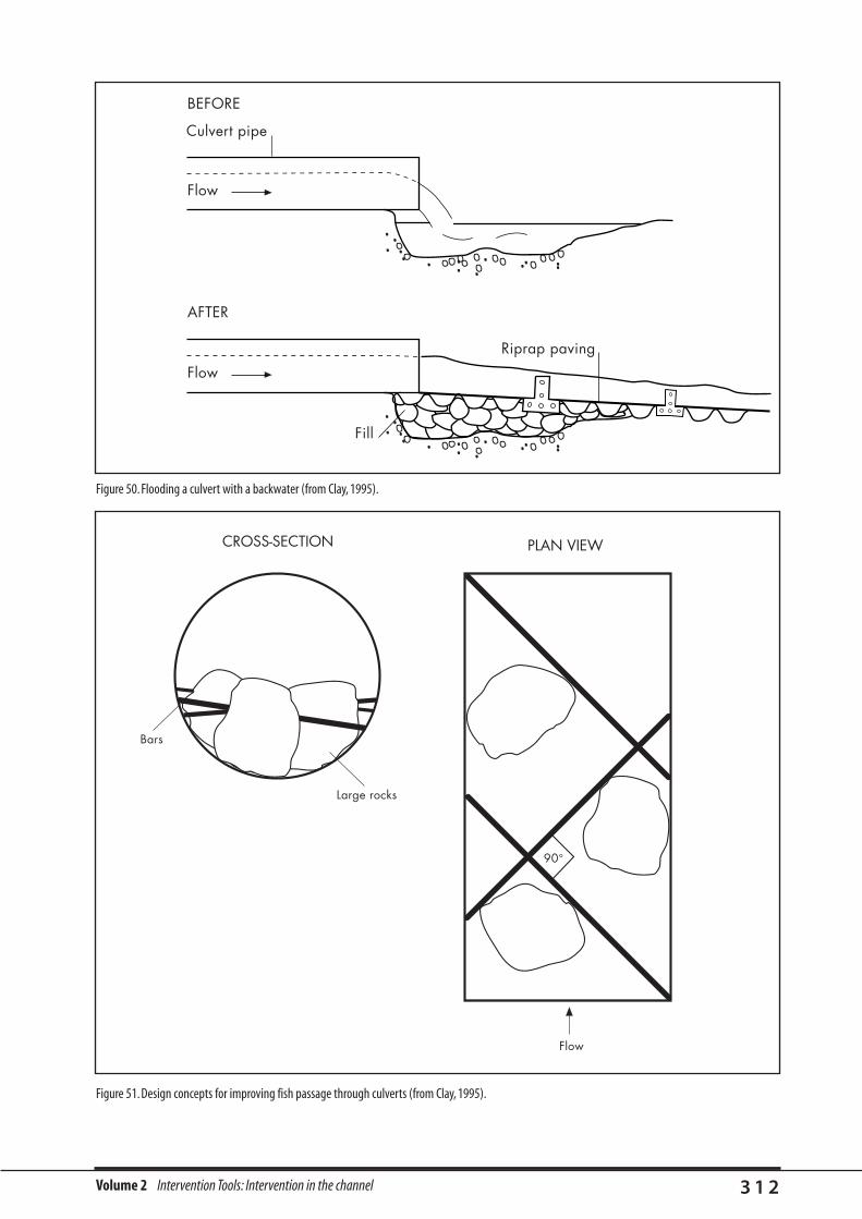
Volume 2 Intervention Tools: Intervention in the channel 3 1 2
CROSS SECTION PLAN VEIW
Bars
Large rocks
Flow
90¡
Culvert pipe
Flow
BEFORE
AFTER
Riprap paving
Fill
Flow
Figure 50. Flooding a culvert with a backwater (from Clay, 1995).
Figure 51. Design concepts for improving fish passage through culverts (from Clay, 1995).
CROSS-SECTION PLAN VIEW

Volume 2 Intervention Tools: Intervention in the channel 3 1 3
MANAGEMENT OF LARGE WOODY DEBRIS
By Christopher Gippel* and Karen White†, with additions by
the editors
1.1. Introduction
Large woody debris (LWD) is recognised as an important
structural and ecological component of many stream
environments. Woody debris provides hard surfaces for
attachment and growth of aquatic plants and
invertebrates, and also habitat conditions of fundamental
importance for maintenance of fish populations (Harmon
et al., 1986; Gippel, 1995). Because many streams have
been de-snagged, or denied a source of woody debris
through degradation or removal of riparian timber, re-
introduction of large woody debris is often an important
aspect of stream rehabilitation. As well as devising
riparian management strategies to ensure an ongoing
supply of wood to streams, some agencies are attempting
to speed the recovery of woody debris loadings by direct
re-introduction of wood and wood structures into
channels (Gippel, 1995).
Re-introduction of woody debris will create physical
habitat, but its utilisation will depend on the existence of
other factors, such as adequate water quality, fish passage,
appropriate stream flows, and recolonisation
opportunities. In Meadow Creek, eastern Oregon, USA,
large amounts of LWD that were re-introduced to the
stream were displaced during a subsequent storm event,
contributing to loss of riparian soils and redistribution of
stream gravels (Beschta et al., 1992). In Fish Creek, north-
central Oregon, despite an extensive instream habitat
rehabilitation effort that included a 200% increase in the
number of pieces of LWD in the channel, the numbers of
anadromous fish did not increase significantly (Beschta et
al., 1992).
Thus, woody debris cannot be introduced in isolation from
other stream rehabilitation strategies.
There is now a reasonable body of literature detailing the
characteristics and loadings of woody debris in rivers,
although most of the work has been done in North
America (eg. Harmon et al., 1986), with a few other studies
from Australasia (eg. Gippel et al., 1996a) and Europe (eg.
Piegay, 1993). These studies provide basic information on
the volumes, dimensions, characteristics and arrangement
of debris found in a range of river environments. Such
information can be useful at the planning stage, but
implementation of a debris re-introduction program
would generally require more detailed information on
issues such as selection of materials, methods of
anchoring (if required), how to build debris structures,
and where to place debris.
Presently, there are no well-established or commonly
accepted criteria for the re-establishment of debris into
rivers. There is only a limited literature dealing with the
methods and results of river rehabilitation projects in
general, and there has been only limited research into the
specific problem of debris re-introduction. Most debris
management guidelines are limited to methods for the
selective removal and/or realignment of debris (Bryant,
1983; Bilby, 1984; Shields and Nunnally, 1984; Gippel, 1995;
Gippel et al., 1996a; Gippel et al., 1996b; Gippel et al., 1998).
Some specific guidelines for debris re-introduction have
recently become available (eg. Gippel et al., 1996b; Abbe et
al., 1997; Ontario Streams, 1998; D’Aoust, 1998;
Hilderbrand et al., 1998). Currently, the design of many
rehabilitation projects tends to be based on a trial-and-
error approach (Brookes and Shields, 1996), and the
1. Re-introduction techniques for instream large woody debris
The artificial reintroduction of LWD into streams should be
seen as a stopgap measure, to be used until a regenerated
riparian zone can naturally supply timber to the stream. In
most cases it will take many decades for trees planted in a
totally cleared riparian zone to grow large enough to
contribute useful long-term LWD.
* Centre for Environmental Applied Hydrology,The University of Melbourne, Parkville,Victoria 3052. Email: [email protected]
† Environmental Scientist, ID&A Pty Ltd, PO Box 5175AA, Melbourne,Victoria 3001. Ph: (03) 9694 1327.

Volume 2 Intervention Tools: Intervention in the channel 3 1 4
re-introduction of debris into rivers seems to be no
exception. Monitoring and post-project evaluation of
rehabilitation works is rarely performed (or if done, it is
rarely reported) (see V.A. Poulin & Associates, 1991;
Beschta et al., 1994; and Gore and Shields, 1995 for some
exceptions); this has no doubt slowed the development of
guidelines.
The majority of the literature on re-introduction of debris
comes from North America. Guidelines devised in North
America may be inappropriate for areas with different types
of trees, or streams that are geomorphologically or
hydrologically different. For example, the eucalypts that line
streams in south-eastern Australia are significantly denser
and stronger than the riparian trees found in North America.
It is more likely then that snags in Australian rivers are more
stable.Additionally, the form of most eucalypts usually
differs from that of North American pines and conifers in
that the bulk of the crown is concentrated towards the top of
the bole, and the bole generally has less taper. Furthermore,
the large branches typical of a eucalyptus tree can effectively
brace the snag in the bed of the river. These differences have
implications for the techniques of anchoring reintroduced
debris. Flows in Australian rivers are highly variable, with
occasional catastrophic floods a feature of the hydrological
regime (Finlayson and McMahon, 1988). Such floods have
sufficient power to significantly re-arrange debris. Bed
material type is probably also important in determining not
only the resistance to debris movement, but also the
tendency of debris to become partially embedded (and thus
more stable). Thus, it is likely that many aspects of debris re-
introduction technology are not directly transferable
between environments.
This section of the manual reviews debris re-introduction
guidelines. Some of these guidelines relate to general
issues that have wide application. Others were developed
from experience in specific areas, and caution is advised in
attempting to transfer them to a geographically different
field site.
Debris is reintroduced to rivers in four main forms:
• as individual debris elements;
• as multi-element debris structures;
• as bank revetment; and
• as in-stream structures such as current deflectors,
weirs, and cover devices.
Much has been written on in-stream structures made
from wood, such as crib walls, deflectors, half-logs and log
weirs (eg. Swales and O’Hara, 1980; Wesche, 1985; DeBano
and Heede, 1987; Charbonneau and Resh, 1992; Gore and
Shields, 1995; Ontario Streams, 1998). These structures
certainly increase the volume of large wood in the stream,
but they are not necessarily expected to perform the same
hydraulic, geomorphic and habitat functions of natural
large woody debris formations. While Booth et al. (1996)
found few analogues for these structures in undisturbed
streams in the Pacific Northwest, natural log steps are a
well-described feature of undisturbed headwater streams
(Heede, 1972; Gurnell and Gregory, 1981; Bilby, 1981;
Harmon et al., 1986). The focus of this review is methods
of re-introducing wood into streams with the specific
objective of rehabilitating or restoring the natural
(pre-disturbance) debris forms and functions. Sometimes
this distinction is unclear; for example, when debris is
re-introduced to provide habitat and to stabilise eroding
banks. Tree revetments are an example of this type of
debris re-introduction (Henderson and Shields, 1984,
p. 60; Wesche, 1985, p. 154; Johnson and Stypula, 1993,
p. 7–22).
Woody material can be obtained in the form of cut logs,
root wads, trunks with attached rootwads or entire trees.
Selection of material and anchoring technique will depend
on the desired function of the debris, the expected life
span of the project, the availability of materials, the costs
involved, and ease of access to the river. The majority of
debris re-introduction projects aim to directly enhance or
restore the natural habitat values provided by wood in
streams (hydraulic diversity; fish cover, resting and refuge
areas; a substrate for macroinvertebrate colonisation)
and/or to indirectly improve habitat by decreasing
sediment discharge downstream and/or protecting banks
from erosion (Skaugset et al., 1994a; Richmond and
Fausch 1995; Booth et al., 1996).
1.2. Suitability of sites for LWD re-introduction
From an ecological perspective ultimate aim is to restore
the natural load of debris into the river. In many instances
this will not be achievable, either because changes of
channel form do not allow it, or because sufficient
quantities of suitable LWD cannot be sourced and
emplaced at reasonable cost. In other cases it may be
undesirable to re-instate the natural load of debris because
of undesirable hydraulic effects (increased flooding), risk
of localised bank erosion, navigational requirements, or

Volume 2 Intervention Tools: Intervention in the channel 3 1 5
excessive risk of damage to infrastructure if the debris
should dislodge.
Snags are not a natural feature of all stream systems.
Streams in the northern tropics, where high gradients and
flows tend to flush out debris, and where high
temperatures result in rapid decomposition of organic
material, may contain low natural levels of wood. Other
streams naturally lacking woody debris include
intermittent desert streams in which vegetation is sparse
and stunted. Organisms in these streams are generally
adapted to alternative habitats such as those provided by
boulders, macrophytes, leaf packs etc.
Most de-snagging has occurred in river systems that drain
the major intensive agricultural regions of Australia. It has
been a common practice—usually as part of a more
general channelisation program—in most larger Victorian
rivers, most coastal New South Wales rivers, the major
rivers and streams of the Murray–Darling basin, almost all
streams running through urban areas in southern
Australia and in several rivers in south-eastern
Queensland and south-western Western Australia.
Swanson et al. (1984) suggested that debris re-
introduction is called for if debris is absent for distances of
5–10 channel widths. However, it should be recognised
that debris is not naturally present in all streams. This may
be due to a lack of riparian trees, but more likely due to a
combination of high stream power and a channel width
that exceeds tree length. In other cases debris could be
buried beneath mobile sand beds. The natural distribution
of LWD has been documented for many sites around the
world, but a general relationship between LWD availability
(proximity, volume, type and dimensions), stream power,
channel width, and LWD loading has not yet been
developed.
For headwater streams in British Columbia,V.A. Poulin &
Associates (1991) recommended that LWD re-introduction
be limited to streams with a gradient <0.03. In lowland
rivers, Sear (1996) found that where bankfull stream
power was below 15 W/m2 habitat-enhancement works
(which might reasonably include LWD re-instatement) are
likely to fail through excessive deposition of sediment.
When bankfull stream power is above 100 W/m2 habitat
enhancement works are likely to fail through excessive
erosion. For lowland streams with bankfull velocities of
0.5–1.5 m/s, and depths of 1–4 m, this suggests an upper
channel gradient limit of 0.02 for slow, shallow streams
and 0.002 for fast, deep streams. Brookes (1990) also noted
that stream rehabilitation works are generally unsuccessful
where the channel confines floods greater than the 1:5 year
ARI event.
1.3. How much debris to put back in?
The natural load of debris into the river can be determined
by measuring the amount of debris present in relatively
natural reaches of a similar river or from records in
historical documents. If no information is available, a
general rule for lowland rivers is to attain a debris loading
of around 0.01 m3 for every m2 of the channel bed (Gippel
et al., 1996). A stream flowing through degraded riparian
land will probably require re-introduction of more debris
than a stream flowing through more intact riparian land.
Booth et al. (1996) commented that debris re-introduction
was particularly appropriate in urban channels, because of
the severe depletion of debris, and because of the general
lack of source material for natural recruitment.
1.4. Replacing individual debris elements
Placement of individual logs is the most common form of
LWD re-introduction. Individual logs may be placed as:
• log steps placed perpendicular to flow in small steep
streams; and
• cross-stream logs placed diagonal or perpendicular to
flow.
As a general rule, the longevity of wood will be greatly
enhanced if it remains fully saturated (Alvarado, 1978;
Harmon et al., 1986). The maximum decay rate occurs
with alternate wetting and drying (Johnson and Stypula,
1993). There are practical difficulties with installation of
debris in deep water. The normal practical limit is around
1.2 m depth (Ontario Streams, 1998).
1.4.1. Log steps
Fallen logs are often incorporated into the geometry of
steep, forested headwater streams, to form natural log
steps (Marston, 1982; DeBano and Heede, 1987). Although
temporary structures, streamside forests maintain the
density of log steps. Artificial re-introduction of log steps
may be appropriate in channels where the riparian forest
has been cleared, or in channels that have stabilised after
incision.

Volume 2 Intervention Tools: Intervention in the channel 3 1 6
Log steps (also termed check dams, low dams or log weirs)
are used in small streams up to 5–6 m wide when
deepening of pools in the range 0.15–0.3 m is desired
(Wesche, 1985). Log steps are often notched in the centre.
This concentrates the flow to form a waterfall, thereby
dissipating energy, aerating the water, and creating a
plunge pool below. Further downstream a riffle forms.
Sediment accumulates above the log steps to produce
gentler channel gradients. Log steps are normally placed in
a step-like series in areas of steep gradient. Stable
pool–riffle sequences are possible in streams with slopes
up to 0.01, and where coarse bed material (coarse sand to
gravel) is present (Swales and O’Hara, 1980). As well as
stabilising the channel bed, log steps can provide pool
habitat for fish and macroinvertebrates (Swales and
O’Hara, 1980; Charbonneau and Resh, 1992; Zapzalka,
1997).Various modifications to the basic single log design
are given by Wesche (1985).
Construction techniques for log steps can be found in
Wesche (1985) and Charbonneau and Resh (1992): log
ends should be sunk 1–2 m, or at least one-third of the
channel width, into both banks; to prevent failure by
undercutting; embed the base log at least 0.15 m into the
substrate; rip-rap can be placed over log ends to reduce
the chance of endcutting; and the minimum log size is 0.3
m diameter. Swales and O’Hara (1980) noted that while the
natural pool–riffle sequence can be re-instated by placing
log steps a distance of 5–7 channel widths apart, the
spacing is often dictated by stream gradient, with steep
streams requiring closer spacings. Montgomery et al.
(1995) found that natural pool spacing in forested
drainage basins decreased from 13 channel widths to less
than one channel width with increasing debris loading.
Life expectancies of 20–40 years can be achieved with
durable timber that is submerged at all times (Wesche,
1985). Minimum design standards for log steps are
provided in Alvarado (1978).
1.4.2. Cross-stream logs
Debris is most commonly re-introduced as a series of
individual logs. There are two basic re-introduction
philosophies: anchored (Ontario Streams, 1998) and
unanchored (Booth et al, 1996). Placement of anchored
individual debris might be the preferred method in areas
where there is concern over the potential for negative
impacts of log jams or debris accumulations. The common
concerns are increased flooding, impediment to fish
passage, catastrophic failure during floods that causes
severe channel erosion (DeBano and Heede, 1987), or drift
accumulations on bridge piers (Diehl, 1997). The need for
anchoring depends to a large extent on the likelihood of
debris movement, which is largely dependent on stream
power, log length and channel width. Hilderbrand et al.
(1998) found that logs longer than the bankfull channel
width were significantly less likely to be displaced than
logs shorter than this width. Ontario Streams (1998) found
that streams wider than 7 m transported debris less than
10 m in length to sites of accumulation, while trees longer
than 10 m were stable if securely anchored to the river bed
or bank. Unanchored debris is placed in streams with the
expectation that it will be re-orientated and relocated
through natural fluvial processes (Booth et al., 1996).
Cross-stream logs are normally placed in small to
moderate-size streams and rivers (5–20 m wide) for the
purpose of providing habitat for fish and
macroinvertebrates, both directly, and indirectly through
the morphological structures that are created by local
hydraulic interactions. Ontario Streams (1998) warned
against attempting to place debris in actively eroding
streams with high bedload transport. Woody debris occurs
naturally at loadings of between 0.001 and 0.1 m3/m2 in
relatively undisturbed streams and rivers. The spacing of
debris is variable, ranging from one log per kilometre to
more than one log per metre in lowland rivers (Gippel et
al., 1996a). Ontario Streams (1998) noted that a density of
12–15 logs per 100 m was not uncommon.V.A Poulin &
Associates (1991) re-introduced debris at a spacing of one
structure for every two bankfull channel widths, based on
Hogan’s (1986) observations of debris density in small
undisturbed streams in the Queen Charlotte Islands,
Canada. Debris is orientated at a range of angles to the
flow. In larger rivers, the debris tends to be orientated
downstream to the flow, at a median angle of around
20–40° to the flow direction (Gippel, 1995). There is little
information regarding the natural position of debris in the
channel, but higher loadings would be expected close to
the banks, as this is both the source of debris and an
anchor point.
There are four main philosophies for placement of debris
within the channel:
• essentially random log placement (Booth et al., 1996;
Hilderbrand et al., 1998);
• placement based on ideas of how to manipulate habitat
(V.A. Poulin & Associates, 1991; Hilderbrand et al., 1998);

Volume 2 Intervention Tools: Intervention in the channel 3 1 7
• placement to mimic natural analogs (Booth et al.,
1996); and
• placement to minimise the hydraulic impact on the
stream with respect to the magnitude of the afflux
generated (Gippel et al., 1996b; Gippel et al., 1998).
Random placement is carried out with the expectation that
the debris will be relocated by subsequent high flows.
Creation of specific habitat features (such as pools)
through strategic debris placement is not well understood,
and trials report variable results (eg.V.A. Poulin &
Associates, 1991; Hilderbrand et al., 1998).
For hydraulic efficiency, debris should be orientated
approximately 20–40° to the flow. In terms of hydraulic
considerations, there is little difference between upstream
and downstream orientation, but downstream orientation
is more common in nature. In lowland Australian streams
the root wad generally faces upstream and the trunk
downstream. (Gippel et al., 1996a; Gippel et al., 1996b;
Gippel et al., 1998). Hydraulic effects can be reduced by
placing debris in zones of low velocity. Ideal locations are
along the channel margin or the inside of meanders or in
pools (Gippel et al., 1998). Debris that occupies less than
10% of the channel cross-sectional area has only a minor
effect on the water surface elevation at bankfull flows.
Higher blockage ratios can cause localised flooding
(Gippel et al., 1996b; Gippel et al., 1998).
1.4.3. Anchored logs
Individual logs can be anchored to bedrock, boulders or
other stable substrate using anchor pins or cable (Ontario
Streams, 1998). The minimum size of debris suitable for
re-introduction is 0.3 m diameter and 3 m length (Ontario
Streams, 1998). Murphy and Koski (1989) preferred logs
greater than 0.6 m in diameter, explaining that smaller
debris is too easily transported to form stable habitat, and
longevity of debris is directly proportional to diameter. In
general, the larger the river, the larger is the debris that is
needed to form stable accumulations (Bisson et al., 1987).
Skaugset et al. (1994a) found that large logs (0.7 m
diameter) placed perpendicular to the flow and flush with
the stream bed (termed ‘spanners’) were the most effective
in pool formation. For habitat creation in small, steep,
degraded streams,V.A. Poulin & Associates (1991) rated
the single cross-stream log orientated diagonally to the
flow and obliquely angled to the bed as the most efficient
structure in terms of cost–benefit ratio. The most
manageable and effective logs were 0.4–0.6 m in diameter
and spanned the width of the channel.
Branches and root wads increase the complexity of
hydraulic interactions, potentially increasing the range of
habitat available (V.A. Poulin & Associates, 1991). Branches
tend to trap other items of debris, so if this is undesirable,
then the branches should be orientated downstream
(Ontario Streams, 1998). Booth et al. (1996) reported that
re-introduced debris with complex geometry was more
effective than simple cylindrical logs in reducing sediment
discharge in unstable channels.
Ontario Streams (1998) recommended the use of aircraft
cable and buried T-bar posts as anchors. Their preferred
configuration was to allow the log to float above the bed.
Millar (1997), Slaney et al. (1997) and D’Aoust (1998)
provide design guidelines for the mass of ballast required
when anchoring debris of various diameters and lengths
with boulders. For example, a single log 0.5 m in diameter
and 10 m long requires 3,600 kg of ballast. The mass of
ballast required is halved if one end of the log is anchored
to a tree or stump on the bank (D’Aoust, 1998).V.A. Poulin
& Associates (1991) used discarded logging cable to attach
debris to stumps or live trees on the bank, or to ‘deadmen’
buried in the substrate. The deadmen were made from
pieces of debris 0.2 m in diameter and 2 m in length,
buried to a depth of 2 m. They also recommended burying
the upstream end of the log flush with the streambed
elevation, or lower, and the downstream end with half of
the log below the bed or lower.
1.4.4. Unanchored logs
There are no guidelines available for re-introduction of
unanchored debris. Booth et al. (1996) determined the size
of material and the number of logs per unit length of
stream on the basis of published descriptions of debris
characteristics in undisturbed streams. The debris was
placed in the stream with the expectation that it would be
re-organised naturally when subjected to high flows.
Hilderbrand et al. (1998) found that logs shorter than the
bankfull channel width moved more frequently than logs
that were longer than the channel width. Long logs moved
less often than short logs, but once entrained, they tended
to move further downstream (Hilderbrand et al., 1998).
1.4.5. Pendants or sweepers
Pendants or sweepers are whole trees anchored by the base
to a stump, steel post or deadman on the bank. Cables are
Volume 2 Intervention Tools: Intervention in the channel 3 1 8
used for the anchoring. The single point of attachment
allows the sweeper to move up and down with flow
variations. Naturally occurring sweepers (sometimes
termed submerged brush shelters) are common in the
upper reaches of Ontario streams (Ontario Streams, 1998).
Whole trees provide a wide range of hydraulic habitat, and
the branches tend to collect fine organic debris, further
adding to the habitat complexity. These structures are
intended to attract juvenile fish by providing dense cover
and a rich food supply (Ontario Streams, 1998).
Sweepers are also used for protecting streambanks from
erosion. Henderson and Shields (1984) reported successful
use of sweepers (they termed them ‘pendants’) that were
placed in an overlapping configuration, cabled to the bank
and to each other. This debris was designed to withstand
velocities of 1.5–2.4 m/s. In another application, sweepers
10–15 m in length were placed 10 m apart, some being
angled downstream from the bank, and others placed
perpendicular from the bank (Henderson and Shields,
1984).
Sweepers are versatile because they can be used in streams
with widely fluctuating water levels and significant
bedload transport (Ontario Streams, 1998). They can be
placed on the outside of meander bends or on straight
reaches. Ontario Streams (1998) recommends a minimum
butt diameter of 0.15–0.40 m and minimum length of 4
m, with a high number of branches being desirable.
1.5. Multi-element debris structures
1.5.1. Clumped debris
Widely spaced individual items of debris have a much
greater hydraulic effect on the flow (in terms of elevation
of the water surface profile) than does a series of closely
spaced logs (preferably within 1 diameter spacing) located
on the bed (Gippel et al., 1996b; Gippel et al., 1998). Debris
can be positioned close together in low clumps to produce
a streamlined long profile shape. A series of closely spaced,
progressively smaller logs upstream and downstream of a
large log will provide a more streamlined shape (Gippel et
al., 1996b; Gippel et al., 1998).
1.5.2. Log arches
Log arches are triangular structures comprising two logs
angled diagonally to the flow, with the upstream ends
cabled together in the centre of the channel and the two
downstream ends anchored on opposite banks. A cross-
brace can be added to the downstream end of the
structure if effective anchoring cannot be achieved. The
apex of the structure is excavated into the stream bed,
flush with the surface of the bed, with the downstream
butt ends buried halfway into the stream bed. These ends
are further secured by cabling them to stumps, trees or
deadmen on the banks. A deadman is buried 2 m deep
into the bed to anchor the apex of the arch (V.A. Poulin &
Associates, 1991).
Millar (1997), Slaney et al. (1997) and D’Aoust (1998)
provide design guidelines for the mass of ballast required
when anchoring log arches of various diameters and
lengths with boulders. For example, up to 6.63 tonnes of
ballast may be required to secure a structure made from
logs 0.5 m diameter and 10 m in length if it is not
anchored to the bank.
V.A. Poulin & Associates (1991) found that, compared with
single cross-stream logs, log arches were more difficult to
build, and prone to unsatisfactory performance in term of
pool development. The main application of log arches is in
situations where the stream is too wide to span with a
single log.
1.5.3. Engineered log jams
Abbe and Montgomery (1996) showed that natural
accumulations of debris in log jams in large alluvial
channels could be extremely stable, with life expectancies
exceeding those of many river engineering projects. Debris
accumulations appear to be more common in undisturbed
rivers in the Pacific Northwest area of the US than they are
in lowland Australian rivers. This partly explained by the
historical removal of log jams from Australian rivers, but it
is also possible that individual logs in Australian streams
are less prone to downstream transport due to their
relatively high wood density (commonly >1,000 kg/m3)
and prominent branches that can become buried in bed
sediments. However, log jams do occur in Australian
streams. Early explorers of the Murray, Murrumbidgee and
Darling rivers often commented on the density of snags in
these rivers, with one surveyor encountering "perfect walls
of timber" (Lloyd, 1988, p. 87–88). There is currently a
large log jam on the Ovens River,Victoria (J. Koehn, pers.
comm.), and there is a 30 km long raft of timber on the
Gwydir River downstream from Moree (McCosker and
Duggin, 1993).

Volume 2 Intervention Tools: Intervention in the channel 3 1 9
Abbe et al. (1997) used the characteristics of naturally
occurring stable log jams, combined with geomorphic and
engineering principles, to develop design guidelines for
engineered log jams (ELJs). These structures are
appropriate in large lowland rivers, and are designed to
provide habitat and to protect banks from erosion. ELJs
are best placed next to pools on the outside bends of
meanders and along the banks of deep runs (Ontario
Streams, 1998).
Design of stable and functional ELJs requires
consideration of the factors that apply to individual LWD
elements, plus some additional factors.
• Rootwad diameter:bankfull discharge water depth > 2
(Abbe et al., 1997).
• Log diameter:bankfull discharge water depth > 0.8
(Abbe et al., 1997).
• Trunk length:rootwad diameter > 3 (Abbe et al., 1997).
• Place the largest logs close to the bank to absorb the
erosive energy of the current (Ontario Streams, 1998).
Position one or more key members parallel to the flow,
with an attached rootwad facing upstream.Various forms
of log jams exist. All types of log jams usually have one or
more key members orientated parallel to the flow, and they
invariably have an attached rootwad facing upstream
(Abbe and Montgomery, 1996).
The key member should be partially buried to provide
stability to the structure. Additional debris should be
racked on top of the key members placed at various
orientations to the flow (Abbe et al., 1997).
The key member and front edge of the ELJ should be
attached to logs (deadmen) that are anchored and keyed
into the bank, and which extend out to the front face of the
structure. These deadmen should face into the bankfull
current, be spaced about 2.5 m apart, and be at least 4–5 m
in length and 0.3 m in diameter (Ontario Streams, 1998).
• The length of an ELJ is site dependent, but varies from
5–30 m (Ontario Streams, 1998).
• The ELJ should not block more than 25% of the low-
flow channel (Ontario Streams, 1998).
• The ELJ should taper up to the bankfull channel
elevation such that it does not impede higher flows
(Ontario Streams, 1998).
1.5.4. Bank revetments and protection
Tree revetments are a relatively inexpensive form of bank
protection. They can also provide suitable habitat for fish
(Gore and Johnson, 1980; Swales and O’Hara, 1980;
Wesche, 1985).
These structures are made from whole trees cabled
together and held in place with rock and/or deadman
anchors buried in the bank (Swales and O’Hara, 1980;
Henderson and Shields, 1984; Wesche, 1985; Johnson and
Stypula, 1993). In the Tanana River, Alaska, a revetment
comprising 51 groups of single and multiple trees was
assembled on the bank, anchored to deadmen, and then
pushed into the stream. The current carried the structure a
short distance downstream and then swung it into the
bank (Henderson and Shields, 1984). Trees lacking root
clumps were less effective than those with root clumps,
because they tended to float away from their original
position.
Tree revetments are pervious, so they can trap sediment.
However, because the timber is subject to wetting and
drying, tree revetments have a limited life and must be
replaced periodically (Johnson and Stypula, 1993).
Henderson and Shields (1984) estimated an effective
lifespan of 10 years for conifer revetments in Wyoming. For
adequate protection of banks on large rivers, the
revetments should be made from bushy trees with a
diameter of approximately 0.3 m (Wesche, 1985; Johnson
and Stypula, 1993). Wesche (1985) reported that a tree
revetment in Oregon reduced mean water velocities near
the bank by about two-thirds, and silt deposits 0.6 m deep
occurred during the first year of placement.
Logs placed at an upstream angle to the flow can enhance
bank stability. Placing logs at an upstream angle to the flow
deflects flows at right angles to the log, away from the bank
and towards the centre of the stream.A series of logs so
placed can shift the thalweg away from the toe of the bank,
thereby enhancing the stability of the riverbank on the
outside of meander bends (Johnson and Stypula, 1993).
Logs placed at a downstream angle to the flow in shallow
water can sometimes result in bank erosion immediately

Volume 2 Intervention Tools: Intervention in the channel 3 2 0
downstream. Placing logs at a downstream angle to the
flow in shallow water can result in localised turbulence
(and scour) around the end of the log, and higher velocity
flow can be directed into the bank immediately
downstream of the log (Johnson and Stypula, 1993).
A bank protection technique commonly used in California
is to incorporate logs into rock toe constructions. Logs are
combined with construction of a rock toe, such that the
rear of the trunk is keyed into the bank in a trench, and the
middle and outer (closest to water) parts of the trunk are
incorporated into the rock toe construction. This
construction technique is commonly used in King County,
Seattle,Washington (Johnson and Stypula, 1993). In this
area, experience has shown that bank stability is enhanced
by placing the rootwad facing upstream into the flow, such
that the snag is orientated at an upstream angle to the flow.
1.6. Selection and sourcing of materials
Selection of debris for re-introduction into streams is
often limited by availability. Logs 6–12 m in length and
0.3–0.8 m in diameter are generally available from
commercial logging operations, but they lack rootwads
and branches (Booth et al., 1996). ELJs can be constructed
largely from logged timber, without branches or large root
wads, thereby reducing sourcing and transport costs.
Rootwads without significant trunks are sometimes
available from land clearing operations (Booth et al.,
1996).
Avoid introduced species such as (in Australia) willows
and poplars, as they decay rapidly and are inappropriate
for invertebrate and biofilm colonisation. In North
America, western red cedar (Thuja plicata) and Sitka
spruce (Picea stichensis) have a greater longevity than
cottonwood (Populus balsamifera) or red alder (Alnus
rubra) (Johnson and Stypula, 1993; Abbe et al., 1997). In
south-eastern Australia, river red gum (Eucalyptus
camaldulensis) has a lower decay coefficient than
mountain ash (Eucalyptus regnans) (Bootle, 1991). Trunk
diameters greater than 0.3 m are preferred, because they
will have greater longevity than smaller pieces (Murphy
and Koski, 1989), and they are stronger and less likely to
fail structurally during large floods.
Fallen debris already present on the floodplain or in the
riparian zone should not be transferred to the stream, as it
performs important functions for the terrestrial
environment (Harmon et al., 1986). Zapzalka (1997)
reported a study in which a tree-thinning experiment was
conducted in six riparian areas in Oregon and Washington.
Two-thirds of the conifers at each site were cut, while the
other third were left as controls. The cut trees were re-
introduced to the streams as woody debris. Rates of
growth in both diameter and height had increased in
treated areas three years after the canopy was thinned,
while an increase in only diameter occurred in untreated
areas (control areas). Three-year mean diameter growth
was 17 mm in areas where the overstorey was removed
compared with only 6 mm in the untreated areas. This
study showed that releasing conifers in small clearings in
riparian zones enhanced conifer survival, thus helping to
contribute to a future supply of conifers to the nearby
stream. This process can significantly contribute to stream
rehabilitation and improve fish habitat (Zapzalka, 1997).
Richmond and Fausch (1995) warn that removal of
riparian trees for placement into streams can result in
soil erosion.
1.7. Planning and undertaking works
Complete in-stream LWD restoration before beginning
riparian restoration. It is inefficient to revegetate the
riparian zone, only to destroy that work by dragging large
logs over the top on their way to the stream.
Work should be done during environmentally less
sensitive periods (eg. not during known periods of fish
spawning) and periods that are likely to present logistical
difficulties, such as high-flow months (Shields and
Nunnally, 1984). House et al. (1989) reported that soil
compaction can result from the use of heavy equipment in
debris re-instatement. Rubber-tyred hydraulic cranes
(Booth et al., 1996), skyline yarding equipment (Skaugset
et al., 1994b) and helicopters (Booth et al., 1996) are
alternative methods of placing debris in streams. In this
respect, ELJs have an advantage over scattered individual
LWD elements because damage to banks during
emplacement is restricted to a smaller number of
locations.
Recently published Australian snag management
guidelines (Gippel et al., 1998) recommend that snag re-
introduction proposals should be treated like any other
development proposal. The proposed work could require
an environmental impact evaluation and public review.
This can be confirmed by the local council. As a minimum,
the proposal should be prepared with a clear set of
objectives, supported by hydraulic calculations.

Volume 2 Intervention Tools: Intervention in the channel 3 2 1
1.8. Conclusion of LWD reinstatement techniques
Debris re-introduction is now accepted as an integral
component of stream rehabilitation programs. In many
cases it is the highest priority action, because of perceived
high benefit–cost ratios and the rapid improvement in
habitat availability that can be achieved. It should be
remembered that re-introduction of debris will not
necessarily result in ecological improvement in terms of
increased fish abundance or diversity, because there are
many other factors that could act to limit fish populations.
Guidelines for re-introduction of large woody debris are
scattered throughout the literature, and some are readily
accessible on the Internet.
In general, the objective should be to reinstate the natural
woody debris loading in a way that mimics the natural
range of sizes and orientations. In some highly modified
streams this may not be possible, in which case the
priority might be channel stability or re-creation of lost
morphological habitat features. The general rule for small
streams appears to be to either place a range of debris in
the channel and allow the stream to reorganise it, or install
a series of individual logs obliquely spanning the channel
and anchored securely on both banks. Anchoring is likely
to be less of an issue in Australia than overseas, because
Australian timber is more durable, dense, and inherently
more stable.
Large rivers require a different approach. The risk of
debris being transported from the site during large floods
and possibly accumulating in undesirable downstream
locations (such as bridge piers) means that debris should
be securely anchored. Clumped debris is more
hydraulically benign than scattered individual elements, so
is the preferred configuration where flooding is a sensitive
issue. Engineered log jams have several advantages over
scattered individual elements. These advantages include:
restriction of bank damage during emplacement to a small
number of locations; log jams are a known focus of
biological activity; ELJs provide bank protection, so that
the requirement for rock protection can be eliminated or
minimised, thereby reducing costs; ELJs are inherently
stable structures; and ELJs can be constructed largely
from logged timber, without branches or large root wads,
thereby reducing sourcing and transport costs.
Note: Reinstating LWD to streams can have consequences for
other values of the stream. Other effects of reinstating large woody
debris, below, discusses the effect of returning snags to streams
on bed and bank erosion, flood levels, and navigation.
(The following section was compiled by the editors)
Reinstating LWD brings three main secondary
consequences for other users of the stream: increased bed
and bank erosion; higher flood peaks and durations; and
problems for navigation. The magnitude of these effects
should be assessed in any plan to reinstate LWD to
streams.
2.1. LWD and channel erosion
2.1.1 Some general principles of LWD and erosion
As with any object placed in a stream, there will be scour
associated with placing LWD into a stream. Much of the
bed scour will be considered welcome habitat. It is usually
the bank erosion that is of most concern to managers.
The following discussion of LWD and channel erosion
applies equally to natural logs in the flow, and logs placed
artificially in the flow. LWD can both increase and decrease
local bank erosion by:
• providing flow resistance in the channel that reduces
average flow velocity, so reducing erosion;
• increasing flow velocity around the snag, thereby
directly increasing bank scour;
• deflecting flow away from the banks, thereby directly
decreasing bank scour;
• directly protecting the banks and reducing erosion; and
• increasing local bed depth and consequently increasing
local bank erosion by slumping.
2. Other effects of reinstating large woody debris
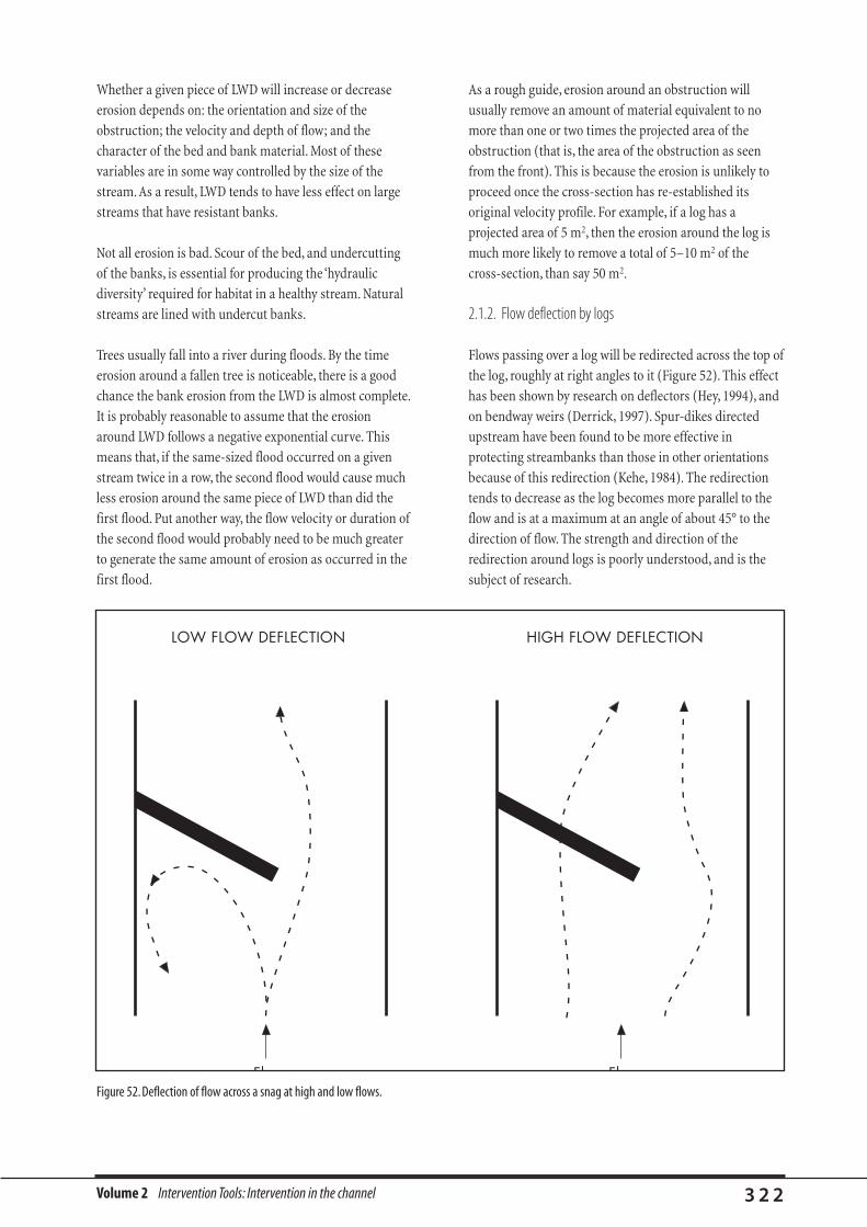
Volume 2 Intervention Tools: Intervention in the channel 3 2 2
Whether a given piece of LWD will increase or decrease
erosion depends on: the orientation and size of the
obstruction; the velocity and depth of flow; and the
character of the bed and bank material. Most of these
variables are in some way controlled by the size of the
stream. As a result, LWD tends to have less effect on large
streams that have resistant banks.
Not all erosion is bad. Scour of the bed, and undercutting
of the banks, is essential for producing the ‘hydraulic
diversity’ required for habitat in a healthy stream. Natural
streams are lined with undercut banks.
Trees usually fall into a river during floods. By the time
erosion around a fallen tree is noticeable, there is a good
chance the bank erosion from the LWD is almost complete.
It is probably reasonable to assume that the erosion
around LWD follows a negative exponential curve. This
means that, if the same-sized flood occurred on a given
stream twice in a row, the second flood would cause much
less erosion around the same piece of LWD than did the
first flood. Put another way, the flow velocity or duration of
the second flood would probably need to be much greater
to generate the same amount of erosion as occurred in the
first flood.
As a rough guide, erosion around an obstruction will
usually remove an amount of material equivalent to no
more than one or two times the projected area of the
obstruction (that is, the area of the obstruction as seen
from the front). This is because the erosion is unlikely to
proceed once the cross-section has re-established its
original velocity profile. For example, if a log has a
projected area of 5 m2, then the erosion around the log is
much more likely to remove a total of 5–10 m2 of the
cross-section, than say 50 m2.
2.1.2. Flow deflection by logs
Flows passing over a log will be redirected across the top of
the log, roughly at right angles to it (Figure 52). This effect
has been shown by research on deflectors (Hey, 1994), and
on bendway weirs (Derrick, 1997). Spur-dikes directed
upstream have been found to be more effective in
protecting streambanks than those in other orientations
because of this redirection (Kehe, 1984). The redirection
tends to decrease as the log becomes more parallel to the
flow and is at a maximum at an angle of about 45° to the
direction of flow. The strength and direction of the
redirection around logs is poorly understood, and is the
subject of research.
Figure 52. Deflection of flow across a snag at high and low flows.
LOW FLOW DEFLECTION HIGH FLOW DEFLECTION
FlFl
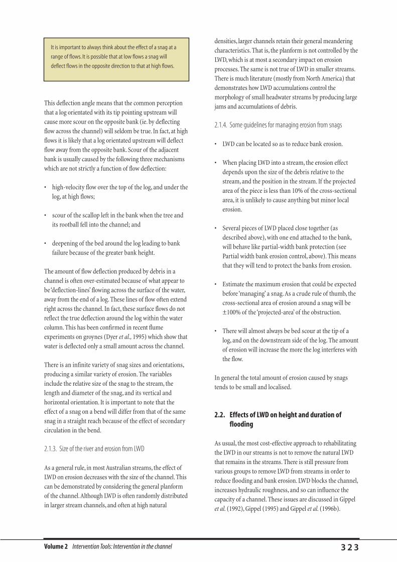
Volume 2 Intervention Tools: Intervention in the channel 3 2 3
This deflection angle means that the common perception
that a log orientated with its tip pointing upstream will
cause more scour on the opposite bank (ie. by deflecting
flow across the channel) will seldom be true. In fact, at high
flows it is likely that a log orientated upstream will deflect
flow away from the opposite bank. Scour of the adjacent
bank is usually caused by the following three mechanisms
which are not strictly a function of flow deflection:
• high-velocity flow over the top of the log, and under the
log, at high flows;
• scour of the scallop left in the bank when the tree and
its rootball fell into the channel; and
• deepening of the bed around the log leading to bank
failure because of the greater bank height.
The amount of flow deflection produced by debris in a
channel is often over-estimated because of what appear to
be ‘deflection-lines’ flowing across the surface of the water,
away from the end of a log. These lines of flow often extend
right across the channel. In fact, these surface flows do not
reflect the true deflection around the log within the water
column. This has been confirmed in recent flume
experiments on groynes (Dyer et al., 1995) which show that
water is deflected only a small amount across the channel.
There is an infinite variety of snag sizes and orientations,
producing a similar variety of erosion. The variables
include the relative size of the snag to the stream, the
length and diameter of the snag, and its vertical and
horizontal orientation. It is important to note that the
effect of a snag on a bend will differ from that of the same
snag in a straight reach because of the effect of secondary
circulation in the bend.
2.1.3. Size of the river and erosion from LWD
As a general rule, in most Australian streams, the effect of
LWD on erosion decreases with the size of the channel. This
can be demonstrated by considering the general planform
of the channel.Although LWD is often randomly distributed
in larger stream channels, and often at high natural
densities, larger channels retain their general meandering
characteristics. That is, the planform is not controlled by the
LWD, which is at most a secondary impact on erosion
processes. The same is not true of LWD in smaller streams.
There is much literature (mostly from North America) that
demonstrates how LWD accumulations control the
morphology of small headwater streams by producing large
jams and accumulations of debris.
2.1.4. Some guidelines for managing erosion from snags
• LWD can be located so as to reduce bank erosion.
• When placing LWD into a stream, the erosion effect
depends upon the size of the debris relative to the
stream, and the position in the stream. If the projected
area of the piece is less than 10% of the cross-sectional
area, it is unlikely to cause anything but minor local
erosion.
• Several pieces of LWD placed close together (as
described above), with one end attached to the bank,
will behave like partial-width bank protection (see
Partial width bank erosion control, above). This means
that they will tend to protect the banks from erosion.
• Estimate the maximum erosion that could be expected
before ‘managing’ a snag. As a crude rule of thumb, the
cross-sectional area of erosion around a snag will be
±100% of the ‘projected-area’ of the obstruction.
• There will almost always be bed scour at the tip of a
log, and on the downstream side of the log. The amount
of erosion will increase the more the log interferes with
the flow.
In general the total amount of erosion caused by snags
tends to be small and localised.
2.2. Effects of LWD on height and duration offlooding
As usual, the most cost-effective approach to rehabilitating
the LWD in our streams is not to remove the natural LWD
that remains in the streams. There is still pressure from
various groups to remove LWD from streams in order to
reduce flooding and bank erosion. LWD blocks the channel,
increases hydraulic roughness, and so can influence the
capacity of a channel. These issues are discussed in Gippel
et al. (1992), Gippel (1995) and Gippel et al. (1996b).
It is important to always think about the effect of a snag at a
range of flows. It is possible that at low flows a snag will
deflect flows in the opposite direction to that at high flows.

Volume 2 Intervention Tools: Intervention in the channel 3 2 4
LWRRDC has also produced snag guidelines. Here we will
provide a little more detail from the above publications.
The hydraulic effects of removing LWD can be considered
as the inverse of putting the timber back into the stream.
Considering how much desnagging has taken place in
Australia, it is surprising how little evaluation there has
been of the effectiveness of the work. The little evaluation
that there is suggests that removing major blockages can
reduce flood levels, but most often because the snags
stabilise the channel. When the snags are removed the bed
deepens and the channel widens. Small streams will be
more affected by desnagging than large ones.
2.2.1. Flooding following the de-snagging of large streams
The following examples illustrate the effect of desnagging
large streams.
One of the major desnagging exercises in recent decades
has been the removal of some 25,000 large river red gum
snags from the Murray River between Hume Weir and
Yarrawonga in order to increase irrigation flow conveyance
(cost about $3 million) (MDBC, 1988). Evaluation of the
work has suggested a 10% increase in conveyance, but this
is questioned by other analyses (Gippel et al., 1992) which
suggest no measurable effect.
Seven LWD accumulations were removed from the Tumut
River (40 m wide, 2.5 m deep) and the effects on flow
conveyance measured (Shields and Gippel, 1995).
Removing the snags reduced upstream water surface level
by about 0.2 m, and increased conveyance by about 20% at
bankfull flow. The afflux extended for about 3 km
upstream. The effect on major floods would be negligible.
Gippel et al. (1996b) also modelled the effect of LWD in the
Lower Thomson River,Victoria and found that 96 items of
woody debris in the channel did not produce a measurable
effect on the height of bankfull flow.
Thus, removing major debris accumulations can increase
channel conveyance, but at high flow the effect would be
trivial in most cases. However, it is also important to note
that stream channels can deepen and widen following de-
snagging, in part because the snags protect the channel
from erosion. This increase in capacity can lead to
substantial increases in channel capacity.
It is important to note that, if flood conveyance is
increased in a reach following de-snagging, then the reach
downstream will probably experience an increase in
flooding. For example, on the Wimmera River, north-
western Victoria, a short reach of stream was bulldozed
clean of all vegetation and snags over a length of about
2,000 m, and the channel enlarged. The works had the
desired effect of reducing the flood duration on six
adjacent properties, but the stream management agency
are now assessing applications from landholders
immediately downstream of the treated reach (whose
properties are now being more flooded) to desnag their
reach of river. The process will continue until all of the
LWD is removed from the stream. Clearly, it is better not to
start the process.
2.2.2. Effect of removing individual logs
Recent research has shown that removing single logs from
a stream will have little effect on flood stage (Gippel et al.,
1996b). This will not be true if the tree is very large in
relation to the channel. A rule of thumb is that a log is not
likely to have a measurable hydraulic effect if it does not
occupy more than 10% of the area of any given cross-
section. Ten percent actually represents a quite high
density of timber.
For example, in a 30 m wide channel, 2 m deep, a log 20 m
long and 1 m in diameter (ie. blocking one third of the
channel area), in a flow of 1.5 m/s, causes a 5% increase in
water surface elevation (100 mm). This is a surprisingly
small effect when you picture the relative size of the log.
Three hydraulically independent items of debris angled at
20–30º produce a combined afflux about the same as a
single log of the same dimensions, orientated
perpendicular to the flow (Gippel et al., 1996b). Another
way of saying this is that the flood effect of a log is
proportional to the projected area that the log presents to
the flow, so three logs at 20º have the same area as one log
going right across the channel (Figure 53).
Several pieces of debris in line will not produce any more
afflux than a single piece, so long as each piece is located
within two times the diameters of the next piece
upstream. Figure 54 shows that up to six pieces can be
Recall (from How changing the channel can affect flooding, in Natural
channel design, this Volume) that de-snagging will have
absolutely no effect if it is carried-out in the backwater of a
larger downstream flow obstruction, such as a bridge.

Volume 2 Intervention Tools: Intervention in the channel 3 2 5
placed in a line. In general, any piece of debris will add
little extra afflux if it is placed within four diameters of the
next piece upstream.
The higher the flow velocity, the greater the impact of LWD
on flood stage. Thus, placing debris away from the centre
line of the channel (on channel edges and point-bars) will
improve channel capacity, but this could also lead to scour
of the channel thalweg.
Gippel et al. (1996b) describes a methodology for
predicting the afflux associated with given pieces of debris
in a stream. This can be used to predict how much flood
benefit you will get by removing LWD. A more
sophisticated approach to predicting the flood impact of
LWD is provided in Shields and Gippel (1995).
2.3. Navigation
A large proportion of the snags in our lowland streams
were removed in order to provide boat access. Returning
snags to streams will affect navigation for some boats. It is
particularly important to consider speed-boats, water
skiers, and canoeists. Hitting a log can be fatal for water-
skiers, as can being stuck under a log for canoeists.
Figure 53.The effect of woody debris on flood levels depends on the logs’ projected area to the flow.The three angled logs have the same effect on flood
levels as the single log.
Figure 54.The rise in water surface level (afflux) caused by cylinders positioned next to each other in a line.The change in water surface level depends on
the spacing of the cylinders (from Gippel et al., 1996b). Reproduced with permission from John Wiley & Sons Ltd.
A B
FlowFlow
20¡
20¡
20¡
2 elements
3 elements
4 elements
5 elements
6 elements
7 elements
Rela
tive
afflu
x (
h/h
)%
0.0
10 2 3 4 5 6 7 8 9 10
0.2
0.4
0.6
0.8
1.0
1.2
1.4
1.6
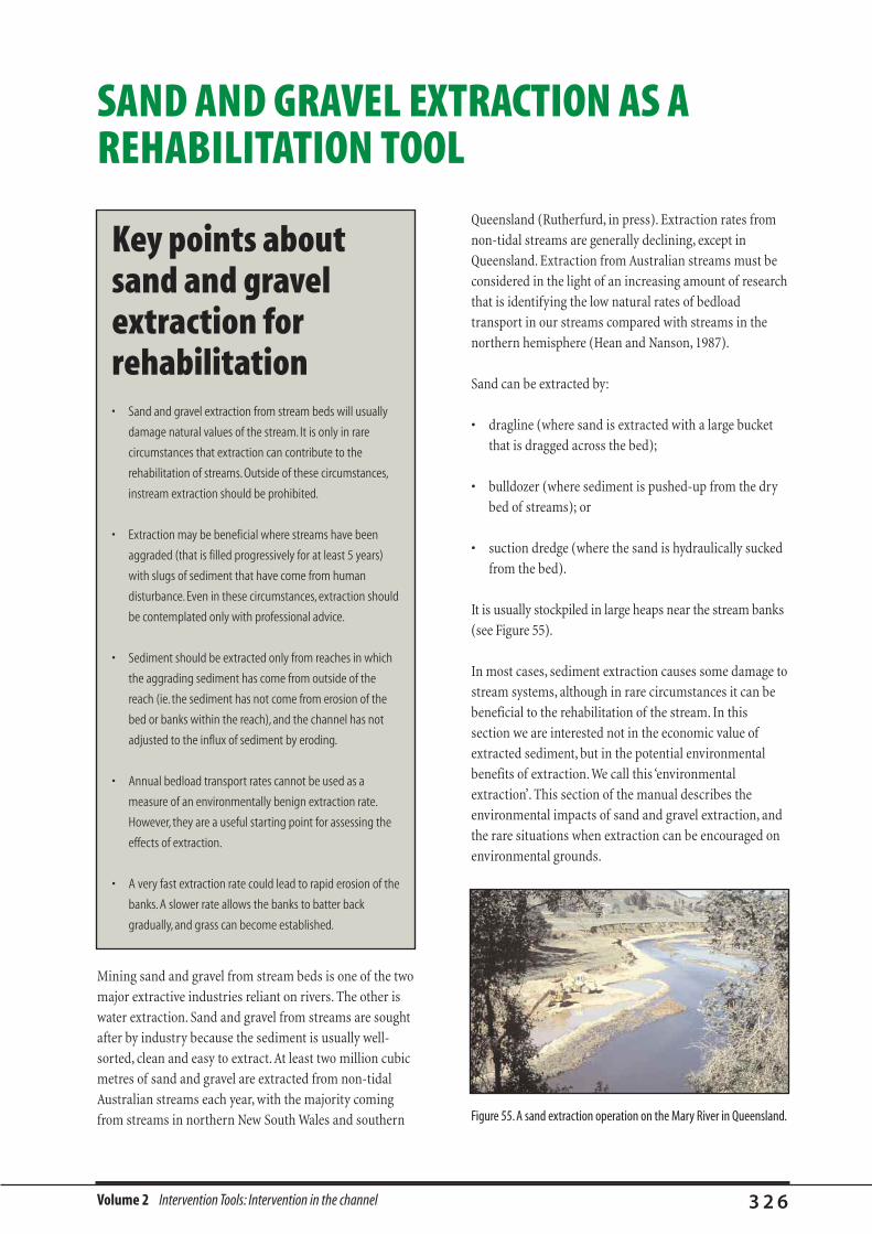
Mining sand and gravel from stream beds is one of the two
major extractive industries reliant on rivers. The other is
water extraction. Sand and gravel from streams are sought
after by industry because the sediment is usually well-
sorted, clean and easy to extract. At least two million cubic
metres of sand and gravel are extracted from non-tidal
Australian streams each year, with the majority coming
from streams in northern New South Wales and southern
Volume 2 Intervention Tools: Intervention in the channel 3 2 6
SAND AND GRAVEL EXTRACTION AS AREHABILITATION TOOL
Key points aboutsand and gravelextraction forrehabilitation• Sand and gravel extraction from stream beds will usually
damage natural values of the stream. It is only in rare
circumstances that extraction can contribute to the
rehabilitation of streams. Outside of these circumstances,
instream extraction should be prohibited.
• Extraction may be beneficial where streams have been
aggraded (that is filled progressively for at least 5 years)
with slugs of sediment that have come from human
disturbance. Even in these circumstances, extraction should
be contemplated only with professional advice.
• Sediment should be extracted only from reaches in which
the aggrading sediment has come from outside of the
reach (ie. the sediment has not come from erosion of the
bed or banks within the reach), and the channel has not
adjusted to the influx of sediment by eroding.
• Annual bedload transport rates cannot be used as a
measure of an environmentally benign extraction rate.
However, they are a useful starting point for assessing the
effects of extraction.
• A very fast extraction rate could lead to rapid erosion of the
banks. A slower rate allows the banks to batter back
gradually, and grass can become established.
Queensland (Rutherfurd, in press). Extraction rates from
non-tidal streams are generally declining, except in
Queensland. Extraction from Australian streams must be
considered in the light of an increasing amount of research
that is identifying the low natural rates of bedload
transport in our streams compared with streams in the
northern hemisphere (Hean and Nanson, 1987).
Sand can be extracted by:
• dragline (where sand is extracted with a large bucket
that is dragged across the bed);
• bulldozer (where sediment is pushed-up from the dry
bed of streams); or
• suction dredge (where the sand is hydraulically sucked
from the bed).
It is usually stockpiled in large heaps near the stream banks
(see Figure 55).
In most cases, sediment extraction causes some damage to
stream systems, although in rare circumstances it can be
beneficial to the rehabilitation of the stream. In this
section we are interested not in the economic value of
extracted sediment, but in the potential environmental
benefits of extraction. We call this ‘environmental
extraction’. This section of the manual describes the
environmental impacts of sand and gravel extraction, and
the rare situations when extraction can be encouraged on
environmental grounds.
Figure 55.A sand extraction operation on the Mary River in Queensland.
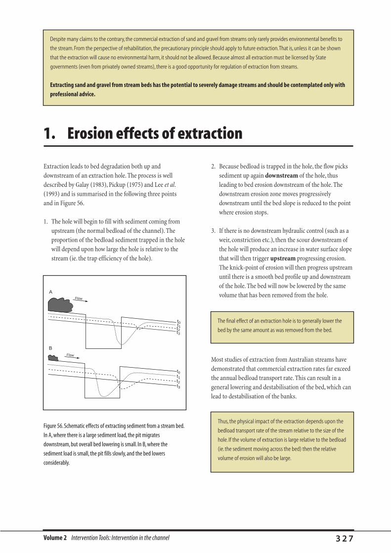
Volume 2 Intervention Tools: Intervention in the channel 3 2 7
Extraction leads to bed degradation both up and
downstream of an extraction hole. The process is well
described by Galay (1983), Pickup (1975) and Lee et al.
(1993) and is summarised in the following three points
and in Figure 56.
1. The hole will begin to fill with sediment coming from
upstream (the normal bedload of the channel). The
proportion of the bedload sediment trapped in the hole
will depend upon how large the hole is relative to the
stream (ie. the trap efficiency of the hole).
Despite many claims to the contrary, the commercial extraction of sand and gravel from streams only rarely provides environmental benefits to
the stream. From the perspective of rehabilitation, the precautionary principle should apply to future extraction.That is, unless it can be shown
that the extraction will cause no environmental harm, it should not be allowed. Because almost all extraction must be licensed by State
governments (even from privately owned streams), there is a good opportunity for regulation of extraction from streams.
Extracting sand and gravel from stream beds has the potential to severely damage streams and should be contemplated only with
professional advice.
2. Because bedload is trapped in the hole, the flow picks
sediment up again downstream of the hole, thus
leading to bed erosion downstream of the hole. The
downstream erosion zone moves progressively
downstream until the bed slope is reduced to the point
where erosion stops.
3. If there is no downstream hydraulic control (such as a
weir, constriction etc.), then the scour downstream of
the hole will produce an increase in water surface slope
that will then trigger upstream progressing erosion.
The knick-point of erosion will then progress upstream
until there is a smooth bed profile up and downstream
of the hole. The bed will now be lowered by the same
volume that has been removed from the hole.
Most studies of extraction from Australian streams have
demonstrated that commercial extraction rates far exceed
the annual bedload transport rate. This can result in a
general lowering and destabilisation of the bed, which can
lead to destabilisation of the banks.
1. Erosion effects of extraction
Figure 56. Schematic effects of extracting sediment from a stream bed.
In A, where there is a large sediment load, the pit migrates
downstream, but overall bed lowering is small. In B, where the
sediment load is small, the pit fills slowly, and the bed lowers
considerably.
Flow
A
t0t1t2t3
t0t1t2t3
Flow
B
The final effect of an extraction hole is to generally lower the
bed by the same amount as was removed from the bed.
Thus, the physical impact of the extraction depends upon the
bedload transport rate of the stream relative to the size of the
hole. If the volume of extraction is large relative to the bedload
(ie. the sediment moving across the bed) then the relative
volume of erosion will also be large.

Volume 2 Intervention Tools: Intervention in the channel 3 2 8
Extraction has numerous secondary physical effects that
have biological consequences. Here are some of them.
• Up and downstream bed degradation. There are many
spectacular examples of bridge and culvert failures
following over-extraction (eg. Galay, 1983; Kondolf,
1994).
• Bed degradation can lead to bank erosion. In one creek,
the same contractor who had the commercial licence to
remove sand from a stream, won the contract to cart
the rock needed to stabilise the banks that were
eroding as a result of over-extraction.
• Coarsening of the bed following bed degradation—the
eroded bed can develop an armour layer of gravels that
may be larger than the armour elsewhere in the
channel. This can affect fish spawning because the
particles become too large for fish to move for egg
laying (Kondolf, 1994).
• Extraction can produce pools in the bed that are large
relative to the average pool depth. These pools can
become stagnant at low flows, with low levels of
dissolved oxygen (MacDonald, 1988) and, because the
pools capture suspended sediment, high nutrient loads.
In lowland Australian streams, deep pools could also
become saline (McGuckin et al., 1991).
• Degradation of the stream bed following extraction can
drop local watertable levels (this may be good or bad
depending on the circumstance, eg. it may drain
important wetlands, or may lower a saline watertable).
• In tidal reaches, bed lowering following extraction can
push the salt-wedge further upstream and alter the
tidal range and velocities (eg. in the Tweed estuary
(Erskine, 1990a) in northern New South
Wales/southern Queensland).
• The extraction process itself may cause many
environmental problems, including damage to the
riparian zone by stockpiles and tracks. The extraction
can also release plumes of suspended sediment to the
stream.
Extraction has direct and indirect biological impacts. These
issues are canvassed in detail in a review of the cumulative
biological effects in Victoria of small-scale eductor dredging
(ie. small suction dredges) (Parliament of Victoria, 1994).
This review concluded that the effects warranted
maintenance of the ban on eductor dredging in the State.
2. Secondary effects of extraction
Many Australian streams are aggrading as a result of
slugs of sediment moving through them. These slugs can
be sand or gravel, and they can originate from many
sources: mining, bank erosion, gully erosion, or (less
commonly) catchment erosion (Figure 57) (sand slugs
are described in more detail in Sediment slugs, in
Common stream problems, this Volume). The slug
migrates down the channel as a wave, and its passing at a
point is seen in a rapid rise followed by a slower fall in
bed level. Sediment slugs can trigger major changes of
channel form as they pass, and they invariably cause
ecological damage.
3. Using extraction to manage sediment slugs
Figure 57. Sand aggrading the Lachlan River (New South Wales)
originating from historical gully and sheet erosion.
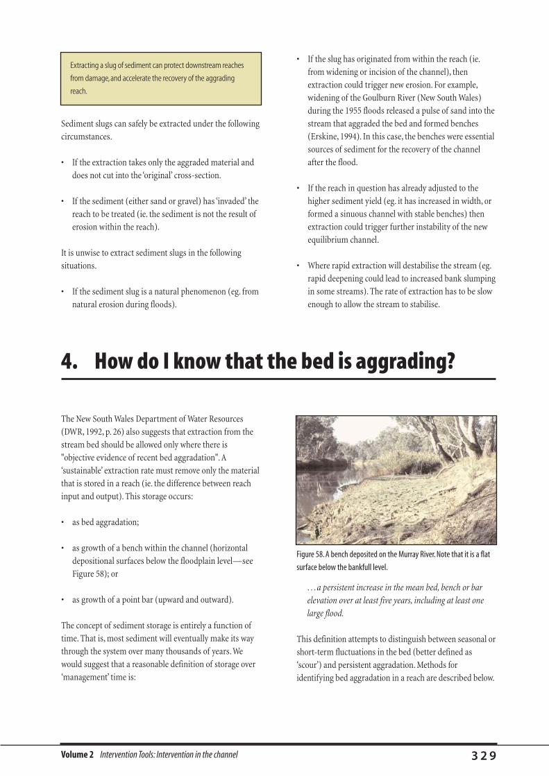
Volume 2 Intervention Tools: Intervention in the channel 3 2 9
Sediment slugs can safely be extracted under the following
circumstances.
• If the extraction takes only the aggraded material and
does not cut into the ‘original’ cross-section.
• If the sediment (either sand or gravel) has ‘invaded’ the
reach to be treated (ie. the sediment is not the result of
erosion within the reach).
It is unwise to extract sediment slugs in the following
situations.
• If the sediment slug is a natural phenomenon (eg. from
natural erosion during floods).
• If the slug has originated from within the reach (ie.
from widening or incision of the channel), then
extraction could trigger new erosion. For example,
widening of the Goulburn River (New South Wales)
during the 1955 floods released a pulse of sand into the
stream that aggraded the bed and formed benches
(Erskine, 1994). In this case, the benches were essential
sources of sediment for the recovery of the channel
after the flood.
• If the reach in question has already adjusted to the
higher sediment yield (eg. it has increased in width, or
formed a sinuous channel with stable benches) then
extraction could trigger further instability of the new
equilibrium channel.
• Where rapid extraction will destabilise the stream (eg.
rapid deepening could lead to increased bank slumping
in some streams). The rate of extraction has to be slow
enough to allow the stream to stabilise.
Extracting a slug of sediment can protect downstream reaches
from damage,and accelerate the recovery of the aggrading
reach.
The New South Wales Department of Water Resources
(DWR, 1992, p. 26) also suggests that extraction from the
stream bed should be allowed only where there is
"objective evidence of recent bed aggradation". A
‘sustainable’ extraction rate must remove only the material
that is stored in a reach (ie. the difference between reach
input and output). This storage occurs:
• as bed aggradation;
• as growth of a bench within the channel (horizontal
depositional surfaces below the floodplain level—see
Figure 58); or
• as growth of a point bar (upward and outward).
The concept of sediment storage is entirely a function of
time. That is, most sediment will eventually make its way
through the system over many thousands of years. We
would suggest that a reasonable definition of storage over
‘management’ time is:
…a persistent increase in the mean bed, bench or bar
elevation over at least five years, including at least one
large flood.
This definition attempts to distinguish between seasonal or
short-term fluctuations in the bed (better defined as
‘scour’) and persistent aggradation. Methods for
identifying bed aggradation in a reach are described below.
4. How do I know that the bed is aggrading?
Figure 58. A bench deposited on the Murray River. Note that it is a flat
surface below the bankfull level.
Volume 2 Intervention Tools: Intervention in the channel 3 3 0
Cross-section surveys
• Repeated cross-section surveys. It is important when
comparing cross-sections to determine that it is
aggradation and not seasonal scour that is being
observed. This depends upon when, and how many
cross-sections are surveyed. For example, in a
particular stream seasonal scour may occur during
winter flows, and deposition during spring flows. If the
cross-sections from winter (scoured bed) are compared
with those from spring, the bed of this stream will
appear to be degrading.
• Cross-sections used for bridge designs are often good
records because they usually show the height and
structure of the bed when the bridge was constructed,
providing reference points for the changes occurring.Bear
in mind that scour may be higher close to the bridge.
• Specific gauge records can provide a long-term record
of bed changes. This is a measure of the stage (that is
water surface height) of a particular water discharge
over time. This stage can be taken from successive
discharge measurements at gauging stations. If the
stage of the same discharge consistently rises, then the
bed could be aggrading. These curves should be
interpreted with caution because there are many
processes that can alter the stage of a river, not just bed
height (eg. width, roughness).
The morphology of the channel itself may give clues. For
example, a tightly meandering channel with a uniform
channel depth (ie. pools filled in) would be unusual in
natural streams and could suggest aggradation.
Anecdotal evidence
There are many sources of anecdotal information that may
be useful in diagnosing aggradation. For example:
• farmers may relate that they have been progressively
shortening their pump take-off pipes over the years as
the bed aggrades; and
• it is very common for landholders to recount that they
used to, for instance, "stand on a horse’s back to collect
swallows eggs under this bridge forty years ago, now
you can’t even crawl under the bridge", or "we used to
swim and fish in a large hole at that bend, that you can
now walk across". It is important to attempt to
corroborate such stories with other evidence because
human memory is not always reliable.
5. Where to extract from?
Sediment can usually be taken from three sites: the active
low-flow channel bed, the point bar (above and below low
water), and from benches. Each site has advantages and
disadvantages.
• Benches should not be extracted, because a proportion
of sediment slugs is often deposited in benches that
can then stabilise. Thus, these benches are an
important part of the recovery of an aggraded stream
and should not be disturbed.
• ‘Skimming’ from a point-bar (ie. removing the point
bar above low water) will lead to downstream erosion,
and might also lead to local erosion of the point-bar
itself upstream of the extraction area. But point-bar
extraction usually will not lead to general upstream
degradation in the reach. At flows around bankfull,
sediment will move across the channel from the
concave bank, and replace the volume of sediment
extracted from the bar. Clear water will then scour
sediment from the next downstream ‘crossing’ (ie.
riffle) and possibly from the next point-bar
downstream.
• Extraction of large volumes from below the low water-
level can be done from point-bars or from the active
channel. Extracting from the point bar will reduce the
continual plumes of sediment moving downstream.
• Extracting at the apex of bends, rather than at
inflection points, could encourage the development of
pools that remain clear of sand. Secondary circulation
at the bends might be sufficient to keep the pool free of
sand once extraction has stopped.
Whichever type of site you extract from, it is usually best
to target the front of the sand wave as it moves
downstream (ie. the downstream end) rather than the tail.
Extracting from the front of the slug will prevent sediment
moving downstream into unaffected reaches.
Volume 2 Intervention Tools: Intervention in the channel 3 3 1
It is useful to have a rough idea of the bed-load transport
rate of a reach in any discussion of extraction. The bed-
load is the coarser fraction of the load that moves by
jumping, rolling, or sliding along the bottom. For example,
if you know that a stream only carries ‘Z’ m3 of sediment a
year, then it is easy to evaluate an extraction proposal for
10 x Z m3/year. Estimating bed-load is a difficult problem.
Fluctuations in bed level are not always a good indication
of bed-load transport rates. There are problems defining
what bed-load is, let alone measuring it.
6.1. Measuring bed-load
There are four ways of estimating bed-load transport rates.
1. Direct measurement. There has been very little
measurement of bed-load transport rates in Australian
rivers. There are numerous ways to measure bed-load,
but the most common is to place a device on the bed of
the stream that will capture the passing bed-load. The
instrument most often used is a Helley-Smith sampler
designed by the United States Geological Survey. The
most thorough bed-load sampling program in
Australia is being carried out with these samplers in
Queensland rivers (see Wong (1994) for details of the
equipment used). Wong estimates that it costs roughly
$30,000 to set up the equipment needed for routine
sampling on one large river. It need not be so expensive
on a small stream, but measurements must be made
frequently and over a long period to be useful.
2. Estimation using equations. There are numerous
equations available for estimating bed-load transport
rates. The equations will give you an answer, but the
problem is to validate the accuracy of the answer. In
general, bed-load estimates from equations are an
imprecise tool and should not be used without expert
interpretation. Different models can provide results that
vary by hundreds of percent and are a poor basis for
decision-making. This is particularly so because the
equations estimate the potential bed-load transport.
This may not be realised if there is not enough supply, as
is often the case in Australia (Hean and Nanson, 1987).
3. Approximation as a function of suspended load. In
the absence of any other measure, a crude way to
estimate bed-load is as a proportion of suspended load.
Many streams in Australia have at least an approximate
record of suspended sediment concentrations because
these are much easier to measure than bed-load. Bed-
load is ‘normally less than 10% of the total solids load,
although in non-alluvial mountain streams it may reach
70%’ (Richards, 1982, p.106).A value of 10% is often
quoted in textbooks. In alluvial rivers, a rule-of-thumb
is that the more similar the bed load and suspended
load in particle size, the higher the bed load as a
proportion of the total load. Lane and Borland (1951)
estimated that bed-load in a sandbed stream, with a
suspended sediment concentration less than 1,000
mg/L, could be between 25% and 100% of the
suspended load. The method is to:
• create a rating curve that relates suspended load to
water discharge;
• estimate annual suspended load from the duration
of flows with particular sediment concentrations;
and
• estimate bed-load as a percentage of suspended load.
You can expect errors of ±200% with this method, but it
may be better than nothing.
4. Deposition in a sediment sink. The best way to
estimate bed-load is to measure the volume of load
entering some type of sink. Examples are:
• sediment volume entering a reservoir in a given time
(difficult to do in a large reservoir). Bed-load will
normally fall out close to the upstream end of the
weir pool. The trap efficiency depends on the size of
the reservoir relative to the discharge, which can be
estimated using the method of Heinemann (1981).
• Another method is to estimate bed-load from how
long it takes to fill an extraction hole below a bed-
control structure of some sort (rock bar or weir).
This works because the extraction hole cannot
trigger upstream progressing degradation. The
methods relies on the bed-load being able to move
easily across the obstruction, and on the hole that it
is entering being large relative to the stream width.
6. How much to extract?
Volume 2 Intervention Tools: Intervention in the channel 3 3 2
The following issues should be considered before
beginning sand and gravel extraction in any stream. Some
of these guidelines are discussed in the New South Wales
policy on extraction from non-tidal watercourses (DWR,
1992).
• If there are assets up or downstream of the extraction
site (eg. bridges, culverts, pipe-crossings), then they
could be threatened if the bed degrades. Bed
degradation may cause bank erosion and thus also
threaten assets such as buildings and roads.
• A good extraction site is one with up and downstream
hardpoints, such as rock bars, that can limit
degradation.
• Sediment should not normally be extracted below low-
flow water level (ie. it should not be ‘skimmed’ from
bars and from seasonally dry beds), except where the
reach is affected by a sand slug (as discussed above).
Even when undertaken above low-flow water level,
sediment skimming can damage the ecology of the
stream by producing a broad, shallow, low-flow channel
that has little habitat potential (Kondolf, 1994).
• If the bed of the stream is armoured, then extraction of
that armour layer could trigger major deepening. This
is because the finer material exposed below the armour
is much more easily eroded than the armour layer
itself. An armour layer often denotes a dominance of
transport capacity over sediment supply. Whether
armour layers should be extracted depends upon how
frequently they are mobilised. For example, the flows
released from Eildon Weir in the Goulburn River in
Victoria are insufficient to transport the sediments
comprising the armour layer in the stream (Erskine
and Terrazzolo, 1996). Extracting the armour layer
could trigger substantial bed degradation because the
sediments beneath the armour layer will then be easily
moved by the flows. If, on the other hand, the armour
layer is moved each year or so in any case, extraction
will have less impact on degradation rates. Note that
even a patchy armour layer can dramatically reduce
bed-load transport.
• Where there is evidence of overall channel enlargement
(ie. substantial bed and bank erosion), then extraction
should not be allowed. Extraction in these
circumstances can jeopardise efforts to rehabilitate
streams. For example, many millions of dollars were
spent ‘training’ the Hunter River in the 1960s and 70s in
order to accelerate the recovery of the channel after
catastrophic widening and erosion in the 1950s. Much
of this recovery was driven by deposition of sediment
in training fences. This process cannot have been
assisted by the commercial extraction of hundreds of
thousands of tonnes of sediment from the channel.
• Extraction increases turbidity in the stream, most
severely during periods of low flow, at the very time
when it is usually easiest to extract. The effect can be
minimised by not extracting from the active channel.
7. Standard rules of any extraction operation
Royalties are often paid to State authorities for extracted
sediment. In Queensland the royalty was little over a dollar
per cubic metre (1995) for extraction from boundary water
courses.A similar royalty applies in Victoria. Considering
that around 28 million cubic metres of sediment has been
extracted from non-tidal Queensland streams between
1950 and 1994 (Queensland Department of Primary
Industries Year Books), the royalties are not trivial.
In a few places, royalties from extraction have been used to
pay for stream rehabilitation works. In the Glenelg River in
Victoria, an extra ‘environmental levy’ of about a dollar per
cubic metre, was placed on the extractors to pay for
rehabilitation, surveys and other costs. On the Nambucca
River in northern New South Wales, extraction royalties
helped to pay for 48 log sills placed in the stream. It has
been suggested that the extraction contributed to the later
failure of some of these structures. Although this assertion
has not been proven, it does highlight the dangers of using
extraction to raise revenue.
Nevertheless, if properly managed, extraction from
appropriate sites can be a useful way of removing damaging
sediment from a stream and raising revenue. This assumes,
of course, that the administrative structure in the State is
flexible enough to return the royalties to the stream.
8. Using extraction to fund stream rehabilitation

Volume 2 Intervention Tools: Intervention in the channel 3 3 3
9. Examples of rehabilitation extraction
Sand slugs in theTambo RiverGold mining in the catchment of the Tambo River,Victoria in
the 1890s produced a pulse of sand that moved into the lower
river within a decade, and then substantially slowed its
progress (Erskine et al., 1990).The front of the sand slug is
progressing slowly (10s–100s of metres per year) toward the
estuary of the river (Figure 59).The estuary is renowned as a
breeding area for the Australian bass (a fish).
At one time the Ports and Harbours Authority attempted to
simultaneously solve two problems by taking sand from the
Tambo sand-slug and placing it on the beaches of the nearby
Lake King (Gippsland Lakes), which were eroding.
Unfortunately, the sand was too fine and washed off the
beaches. If the strategy had worked, it would have been a neat
example of rehabilitation.
The Tambo slug is ideal for ‘environmental extraction’ because:
• the sand has come from outside the reach in question;
• the bed has been aggraded for more than five years (in fact,
for nearly a century);
• the reach of the Tambo that has filled with sand has not
adjusted to the slug of sand (it has simply aggraded
without widening); and
• the further downstream migration of the sand is set to
cause further environmental problems (threatening a
native fish species).
Sand slugs in theGlenelg River,western VictoriaCatchment and gully erosion in the catchment of the Glenelg
River last century released slugs of sand into first the
tributaries, then the trunk stream of the river. An estimated 4–8
million m3 of sediment is stored in the system.The sand is
considered the major environmental threat to the river (Ian
Drummond and Associates et al., 1992).
The sand is moving only slowly (ie. about 0.1% to 0.05% of the
total storage per year) through the system and one option for
management is its commercial extraction.There is a good
demand for quartz sand in the region. A management plan was
developed for the catchment that identifies how much sand
should be removed from particular reaches (Rutherfurd and
Budahazy, 1996).The sand in the catchment is actually made
up of several discrete slugs that were identified by probing
with a 5 m steel probe.The clay bed of the river could be
identified easily below the sand.
The bed-load transport rate in the trunk and tributary streams
was estimated by various methods.These rates were used to
identify the minimum rate of extraction required to protect
downstream reaches.
Extraction was encouraged from the front end of particular slugs
in order to protect remnant reaches of stream that have not yet
been damaged by the creeping sand (ie.extract upstream of
these reaches to intercept the sand). In smaller streams the rate
of extraction was restricted because of the bank erosion that
would be caused by a rapid fall in the level of sand.
Figure 59.The front of the sand slug in the Tambo River (see arrow)
(the water is about 5 m deep downstream of the front of the slug).

Volume 2 Intervention Tools: Intervention in the channel 3 3 4
We conclude this section by reiterating that there are so many
physical and biological problems associated with extraction of
sand or gravel from stream beds that the practice should be
discouraged. Nevertheless, in some circumstances, such as
where a stream bed is rapidly aggrading with a pulse (or slug)
of sediment, extraction might deliver environmental benefits.

INTERVENTION IN THERIPARIAN ZONE
• Vegetation management
• Exotic weed infested streams
• Willow infested streams
• Managing stock access to streams
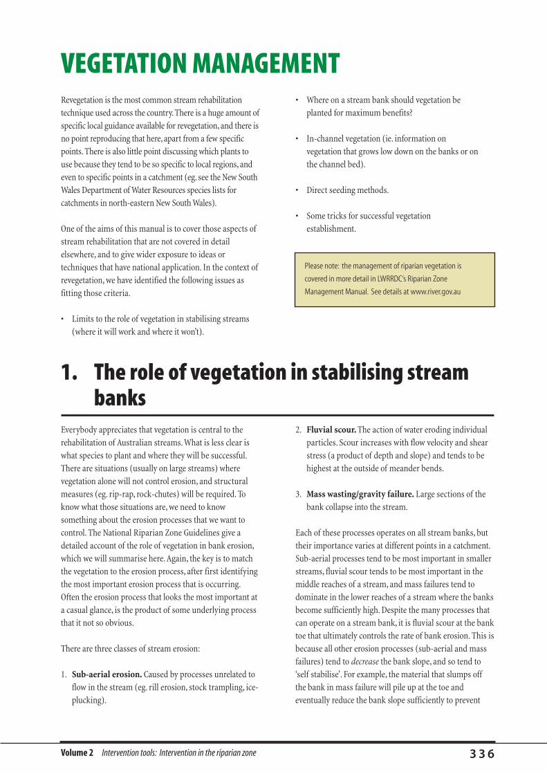
Volume 2 Intervention tools: Intervention in the riparian zone 3 3 6
Revegetation is the most common stream rehabilitation
technique used across the country. There is a huge amount of
specific local guidance available for revegetation, and there is
no point reproducing that here, apart from a few specific
points. There is also little point discussing which plants to
use because they tend to be so specific to local regions, and
even to specific points in a catchment (eg. see the New South
Wales Department of Water Resources species lists for
catchments in north-eastern New South Wales).
One of the aims of this manual is to cover those aspects of
stream rehabilitation that are not covered in detail
elsewhere, and to give wider exposure to ideas or
techniques that have national application. In the context of
revegetation, we have identified the following issues as
fitting those criteria.
• Limits to the role of vegetation in stabilising streams
(where it will work and where it won’t).
• Where on a stream bank should vegetation be
planted for maximum benefits?
• In-channel vegetation (ie. information on
vegetation that grows low down on the banks or on
the channel bed).
• Direct seeding methods.
• Some tricks for successful vegetation
establishment.
VEGETATION MANAGEMENT
Everybody appreciates that vegetation is central to the
rehabilitation of Australian streams. What is less clear is
what species to plant and where they will be successful.
There are situations (usually on large streams) where
vegetation alone will not control erosion, and structural
measures (eg. rip-rap, rock-chutes) will be required. To
know what those situations are, we need to know
something about the erosion processes that we want to
control. The National Riparian Zone Guidelines give a
detailed account of the role of vegetation in bank erosion,
which we will summarise here. Again, the key is to match
the vegetation to the erosion process, after first identifying
the most important erosion process that is occurring.
Often the erosion process that looks the most important at
a casual glance, is the product of some underlying process
that it not so obvious.
There are three classes of stream erosion:
1. Sub-aerial erosion. Caused by processes unrelated to
flow in the stream (eg. rill erosion, stock trampling, ice-
plucking).
2. Fluvial scour. The action of water eroding individual
particles. Scour increases with flow velocity and shear
stress (a product of depth and slope) and tends to be
highest at the outside of meander bends.
3. Mass wasting/gravity failure. Large sections of the
bank collapse into the stream.
Each of these processes operates on all stream banks, but
their importance varies at different points in a catchment.
Sub-aerial processes tend to be most important in smaller
streams, fluvial scour tends to be most important in the
middle reaches of a stream, and mass failures tend to
dominate in the lower reaches of a stream where the banks
become sufficiently high. Despite the many processes that
can operate on a stream bank, it is fluvial scour at the bank
toe that ultimately controls the rate of bank erosion. This is
because all other erosion processes (sub-aerial and mass
failures) tend to decrease the bank slope, and so tend to
‘self stabilise’. For example, the material that slumps off
the bank in mass failure will pile up at the toe and
eventually reduce the bank slope sufficiently to prevent
1. The role of vegetation in stabilising stream banks
Please note: the management of riparian vegetation is
covered in more detail in LWRRDC‘s Riparian Zone
Management Manual. See details at www.river.gov.au

Volume 2 Intervention tools: Intervention in the riparian zone 3 3 7
further slumps. However, if fluvial scour removes the
collapsed material, then the banks remain steep and
unstable. Thus, it is the fluvial scour at the bank toe that
keeps the banks unstable (Thorne, 1982).
1.1. How vegetation stabilises banks
Vegetation reduces erosion in the following ways:
1. Sub-aerial erosion. Vegetation growing on the bank, or
hanging over the bank, protects the bank from erosion
due to rain-splash and most sub-aerial processes.
2. Fluvial scour. Vegetation growing on a bank face
dramatically reduces the flow velocity close to the bank,
and directly reduces scour (Thorne and Furbish, 1995).
The vegetation also directly strengthens bank material,
making it harder to remove from the bank face.
3. Mass failure. The most important role of vegetation in
mass failure is to reinforce the failure plane (ie. where
roots pass through the failure plane).Vegetation has
other effects on mass failure, such as altering bank
hydrology, but these tend to be less important than root
reinforcement. For example, people are often concerned
about the effects of the added weight of a tree on the
bank. This is very seldom a problem. In fact, the weight
of the tree will often reduce mass failure, especially if it
is planted low on the bank face.
1.2. Where to plant vegetation on the bank
If you have identified that a specific erosion process is
dominant then adopt the more specific rules that follow:
1. Sub-aerial erosion. Any vegetation on the bank face,
or hanging over the bank face is suitable.
2. Fluvial scour. Again, any vegetation on the bank face
is best. Particularly good are macrophytes that will
grow close to the toe (see In-channel vegetation:
macrophytes and emergent plants below).Vegetation on
the bank top is unlikely to do much for this process,
except in large floods when it slows the overbank flow.
3. Mass failure. Roots need to cross the failure plane to
be effective. The failure plane is the fracture line where
the slump block breaks away from the bank.You can
estimate the depth of the failure plane by looking at
typical failure blocks along the reach, and by looking
for tension cracks on top of the bank. The failure plane
will be either steeper than the bank face, or will parallel
the face. The best place to plant trees to control mass
failure is close to the bank toe. The next best place is
close to the potential failure plane, on top of the bank.
Shallow-rooted species on the bank face are useful for
controlling shallow slips.
1.3. Limits to the role of vegetation
Vegetation is not the answer to all stream erosion
problems. It has its limitations and in that regard the
following three points need to be kept in mind.
1. Before European settlement, even with a full cover of
native vegetation, streams eroded their banks, and
underwent major changes of channel form and
position. The evidence for such changes is preserved as
ancient channels and other features on our floodplains.
Thus, vegetation alone will not eliminate bank erosion,
if that is your goal. In fact some of the erosion
associated with vegetation, such as undercutting, is
thought to be desirable fish habitat.
2. Clearing of vegetation, and other European
modifications, have greatly increased the ‘power’ of our
streams. That is, over the last 150 years many of our
streams have deepened and enlarged so that they now
carry a higher proportion of water in the channel than
on the floodplain. This fundamental transformation of
our streams cannot be reversed by simply returning
vegetation to the stream. In many cases, the forces now
operating in our transformed channels are too great for
vegetation to modify.
For bank erosion and vegetation the key questions to ask are:
What is the dominant erosion process? Can it be controlled
using the vegetation that I have at my disposal? Often these
questions come down to whether you can establish
vegetation on the bank face, and whether you can get roots
close to the bank toe.
The simple rule for planting vegetation for bank stability is to
get it as close as possible to the low- water level, and to have
as much of it as possible.
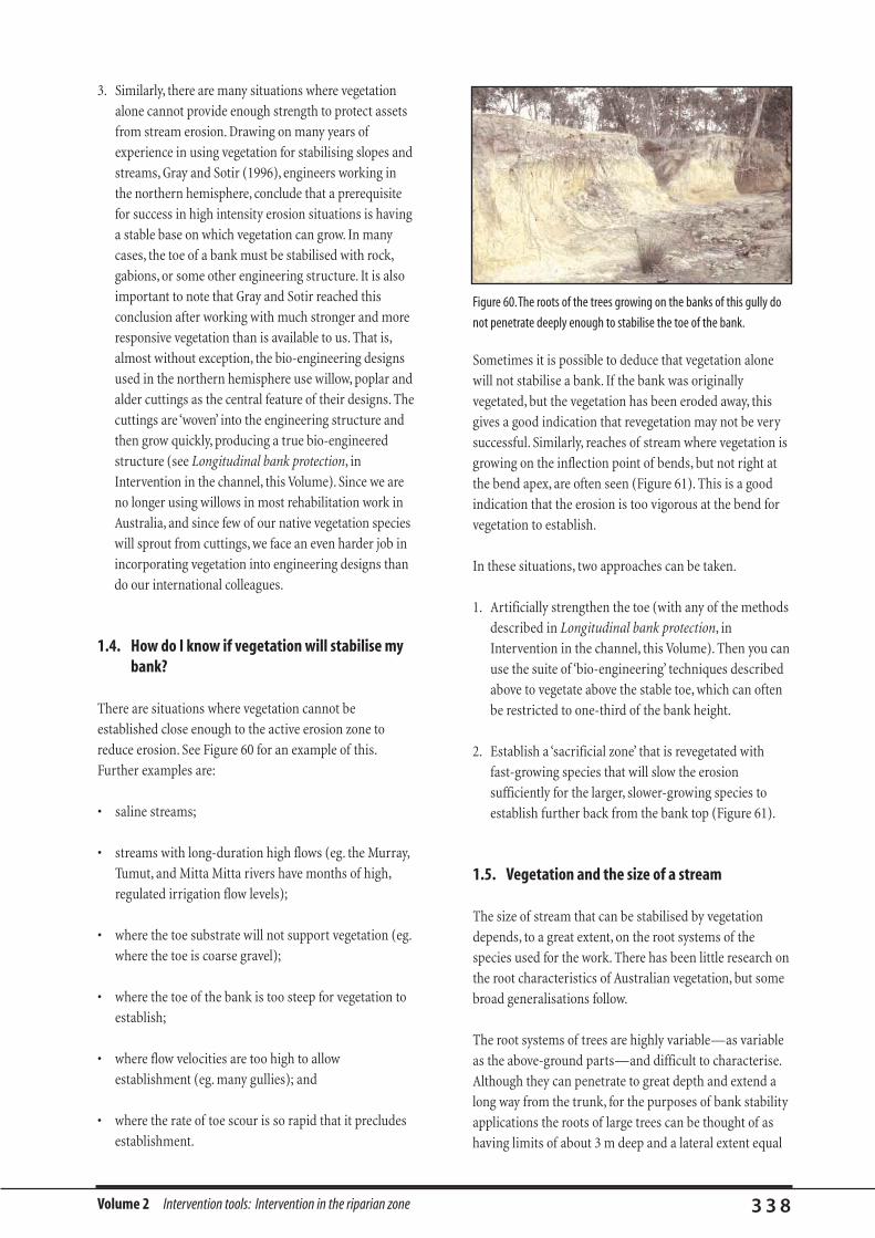
Volume 2 Intervention tools: Intervention in the riparian zone 3 3 8
3. Similarly, there are many situations where vegetation
alone cannot provide enough strength to protect assets
from stream erosion. Drawing on many years of
experience in using vegetation for stabilising slopes and
streams, Gray and Sotir (1996), engineers working in
the northern hemisphere, conclude that a prerequisite
for success in high intensity erosion situations is having
a stable base on which vegetation can grow. In many
cases, the toe of a bank must be stabilised with rock,
gabions, or some other engineering structure. It is also
important to note that Gray and Sotir reached this
conclusion after working with much stronger and more
responsive vegetation than is available to us. That is,
almost without exception, the bio-engineering designs
used in the northern hemisphere use willow, poplar and
alder cuttings as the central feature of their designs. The
cuttings are ‘woven’ into the engineering structure and
then grow quickly, producing a true bio-engineered
structure (see Longitudinal bank protection, in
Intervention in the channel, this Volume). Since we are
no longer using willows in most rehabilitation work in
Australia, and since few of our native vegetation species
will sprout from cuttings, we face an even harder job in
incorporating vegetation into engineering designs than
do our international colleagues.
1.4. How do I know if vegetation will stabilise mybank?
There are situations where vegetation cannot be
established close enough to the active erosion zone to
reduce erosion. See Figure 60 for an example of this.
Further examples are:
• saline streams;
• streams with long-duration high flows (eg. the Murray,
Tumut, and Mitta Mitta rivers have months of high,
regulated irrigation flow levels);
• where the toe substrate will not support vegetation (eg.
where the toe is coarse gravel);
• where the toe of the bank is too steep for vegetation to
establish;
• where flow velocities are too high to allow
establishment (eg. many gullies); and
• where the rate of toe scour is so rapid that it precludes
establishment.
Sometimes it is possible to deduce that vegetation alone
will not stabilise a bank. If the bank was originally
vegetated, but the vegetation has been eroded away, this
gives a good indication that revegetation may not be very
successful. Similarly, reaches of stream where vegetation is
growing on the inflection point of bends, but not right at
the bend apex, are often seen (Figure 61). This is a good
indication that the erosion is too vigorous at the bend for
vegetation to establish.
In these situations, two approaches can be taken.
1. Artificially strengthen the toe (with any of the methods
described in Longitudinal bank protection, in
Intervention in the channel, this Volume). Then you can
use the suite of ‘bio-engineering’ techniques described
above to vegetate above the stable toe, which can often
be restricted to one-third of the bank height.
2. Establish a ‘sacrificial zone’ that is revegetated with
fast-growing species that will slow the erosion
sufficiently for the larger, slower-growing species to
establish further back from the bank top (Figure 61).
1.5. Vegetation and the size of a stream
The size of stream that can be stabilised by vegetation
depends, to a great extent, on the root systems of the
species used for the work. There has been little research on
the root characteristics of Australian vegetation, but some
broad generalisations follow.
The root systems of trees are highly variable—as variable
as the above-ground parts—and difficult to characterise.
Although they can penetrate to great depth and extend a
long way from the trunk, for the purposes of bank stability
applications the roots of large trees can be thought of as
having limits of about 3 m deep and a lateral extent equal
Figure 60.The roots of the trees growing on the banks of this gully do
not penetrate deeply enough to stabilise the toe of the bank.
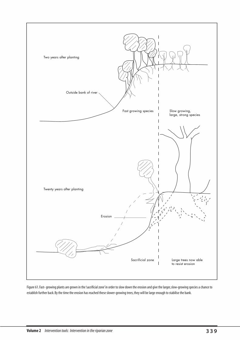
Volume 2 Intervention tools: Intervention in the riparian zone 3 3 9
Figure 61. Fast- growing plants are grown in the ‘sacrificial zone’ in order to slow down the erosion and give the larger, slow-growing species a chance to
establish further back. By the time the erosion has reached these slower-growing trees, they will be large enough to stabilise the bank.
Two years after planting
Twenty years after planting
Sacrificial zone Large trees now able to resist erosion
Fast growing species Slow growing,large, strong species
Erosion
Outside bank of river
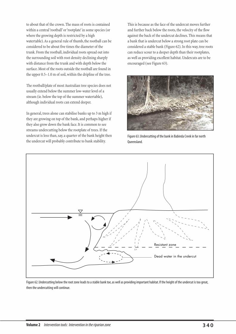
Volume 2 Intervention tools: Intervention in the riparian zone 3 4 0
to about that of the crown. The mass of roots is contained
within a central ‘rootball’ or ‘rootplate’ in some species (or
where the growing depth is restricted by a high
watertable). As a general rule of thumb, the rootball can be
considered to be about five times the diameter of the
trunk. From the rootball, individual roots spread out into
the surrounding soil with root density declining sharply
with distance from the trunk and with depth below the
surface. Most of the roots outside the rootball are found in
the upper 0.5–1.0 m of soil, within the dripline of the tree.
The rootball/plate of most Australian tree species does not
usually extend below the summer low-water level of a
stream (ie. below the top of the summer watertable),
although individual roots can extend deeper.
In general, trees alone can stabilise banks up to 3 m high if
they are growing on top of the bank, and perhaps higher if
they also grow down the bank face. It is common to see
streams undercutting below the rootplate of trees. If the
undercut is less than, say, a quarter of the bank height then
the undercut will probably contribute to bank stability.
This is because as the face of the undercut moves further
and further back below the roots, the velocity of the flow
against the back of the undercut declines. This means that
a bank that is undercut below a strong root plate can be
considered a stable bank (Figure 62). In this way, tree roots
can reduce scour to a deeper depth than their rootplates,
as well as providing excellent habitat. Undercuts are to be
encouraged (see Figure 63).
Figure 63. Undercutting of the bank in Babinda Creek in far north
Queensland.
Dead water in the undercut
Resistant zone
Figure 62. Undercutting below the root zone leads to a stable bank toe, as well as providing important habitat. If the height of the undercut is too great,
then the undercutting will continue.
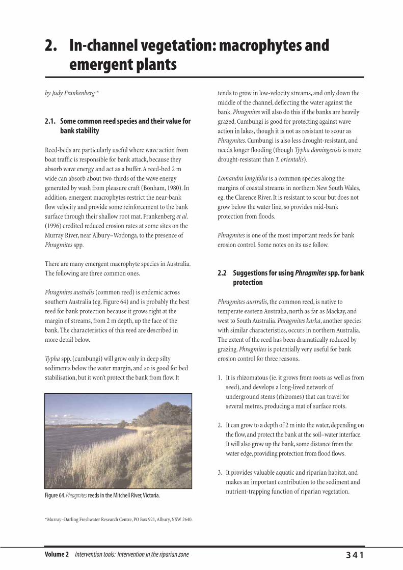
Volume 2 Intervention tools: Intervention in the riparian zone 3 4 1
by Judy Frankenberg *
2.1. Some common reed species and their value forbank stability
Reed-beds are particularly useful where wave action from
boat traffic is responsible for bank attack, because they
absorb wave energy and act as a buffer. A reed-bed 2 m
wide can absorb about two-thirds of the wave energy
generated by wash from pleasure craft (Bonham, 1980). In
addition, emergent macrophytes restrict the near-bank
flow velocity and provide some reinforcement to the bank
surface through their shallow root mat. Frankenberg et al.
(1996) credited reduced erosion rates at some sites on the
Murray River, near Albury–Wodonga, to the presence of
Phragmites spp.
There are many emergent macrophyte species in Australia.
The following are three common ones.
Phragmites australis (common reed) is endemic across
southern Australia (eg. Figure 64) and is probably the best
reed for bank protection because it grows right at the
margin of streams, from 2 m depth, up the face of the
bank. The characteristics of this reed are described in
more detail below.
Typha spp. (cumbungi) will grow only in deep silty
sediments below the water margin, and so is good for bed
stabilisation, but it won’t protect the bank from flow. It
tends to grow in low-velocity streams, and only down the
middle of the channel, deflecting the water against the
bank. Phragmites will also do this if the banks are heavily
grazed. Cumbungi is good for protecting against wave
action in lakes, though it is not as resistant to scour as
Phragmites. Cumbungi is also less drought-resistant, and
needs longer flooding (though Typha domingensis is more
drought-resistant than T. orientalis).
Lomandra longifolia is a common species along the
margins of coastal streams in northern New South Wales,
eg. the Clarence River. It is resistant to scour but does not
grow below the water line, so provides mid-bank
protection from floods.
Phragmites is one of the most important reeds for bank
erosion control. Some notes on its use follow.
2.2 Suggestions for using Phragmites spp. for bankprotection
Phragmites australis, the common reed, is native to
temperate eastern Australia, north as far as Mackay, and
west to South Australia. Phragmites karka, another species
with similar characteristics, occurs in northern Australia.
The extent of the reed has been dramatically reduced by
grazing. Phragmites is potentially very useful for bank
erosion control for three reasons.
1. It is rhizomatous (ie. it grows from roots as well as from
seed), and develops a long-lived network of
underground stems (rhizomes) that can travel for
several metres, producing a mat of surface roots.
2. It can grow to a depth of 2 m into the water, depending on
the flow, and protect the bank at the soil–water interface.
It will also grow up the bank, some distance from the
water edge, providing protection from flood flows.
3. It provides valuable aquatic and riparian habitat, and
makes an important contribution to the sediment and
nutrient-trapping function of riparian vegetation.
2. In-channel vegetation: macrophytes and emergent plants
Figure 64. Phragmites reeds in the Mitchell River,Victoria.
*Murray–Darling Freshwater Research Centre, PO Box 921, Albury, NSW 2640.
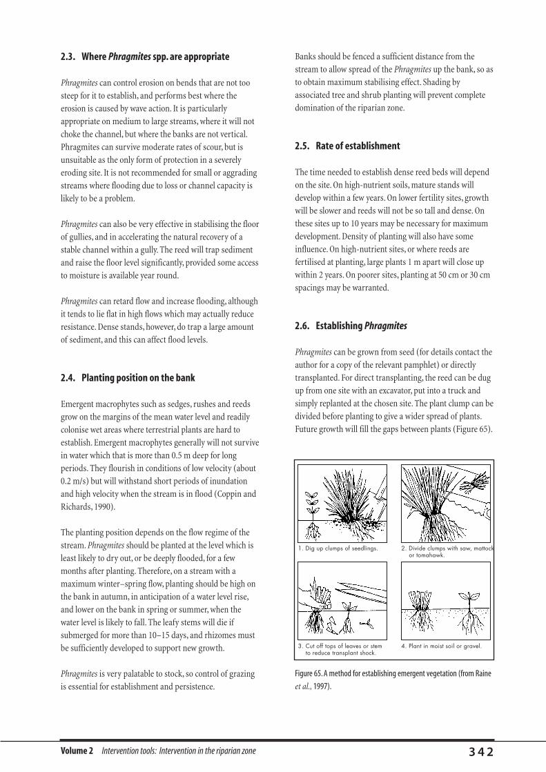
Volume 2 Intervention tools: Intervention in the riparian zone 3 4 2
2.3. Where Phragmites spp. are appropriate
Phragmites can control erosion on bends that are not too
steep for it to establish, and performs best where the
erosion is caused by wave action. It is particularly
appropriate on medium to large streams, where it will not
choke the channel, but where the banks are not vertical.
Phragmites can survive moderate rates of scour, but is
unsuitable as the only form of protection in a severely
eroding site. It is not recommended for small or aggrading
streams where flooding due to loss or channel capacity is
likely to be a problem.
Phragmites can also be very effective in stabilising the floor
of gullies, and in accelerating the natural recovery of a
stable channel within a gully. The reed will trap sediment
and raise the floor level significantly, provided some access
to moisture is available year round.
Phragmites can retard flow and increase flooding, although
it tends to lie flat in high flows which may actually reduce
resistance. Dense stands, however, do trap a large amount
of sediment, and this can affect flood levels.
2.4. Planting position on the bank
Emergent macrophytes such as sedges, rushes and reeds
grow on the margins of the mean water level and readily
colonise wet areas where terrestrial plants are hard to
establish. Emergent macrophytes generally will not survive
in water which that is more than 0.5 m deep for long
periods. They flourish in conditions of low velocity (about
0.2 m/s) but will withstand short periods of inundation
and high velocity when the stream is in flood (Coppin and
Richards, 1990).
The planting position depends on the flow regime of the
stream. Phragmites should be planted at the level which is
least likely to dry out, or be deeply flooded, for a few
months after planting. Therefore, on a stream with a
maximum winter–spring flow, planting should be high on
the bank in autumn, in anticipation of a water level rise,
and lower on the bank in spring or summer, when the
water level is likely to fall. The leafy stems will die if
submerged for more than 10–15 days, and rhizomes must
be sufficiently developed to support new growth.
Phragmites is very palatable to stock, so control of grazing
is essential for establishment and persistence.
Banks should be fenced a sufficient distance from the
stream to allow spread of the Phragmites up the bank, so as
to obtain maximum stabilising effect. Shading by
associated tree and shrub planting will prevent complete
domination of the riparian zone.
2.5. Rate of establishment
The time needed to establish dense reed beds will depend
on the site. On high-nutrient soils, mature stands will
develop within a few years. On lower fertility sites, growth
will be slower and reeds will not be so tall and dense. On
these sites up to 10 years may be necessary for maximum
development. Density of planting will also have some
influence. On high-nutrient sites, or where reeds are
fertilised at planting, large plants 1 m apart will close up
within 2 years. On poorer sites, planting at 50 cm or 30 cm
spacings may be warranted.
2.6. Establishing Phragmites
Phragmites can be grown from seed (for details contact the
author for a copy of the relevant pamphlet) or directly
transplanted. For direct transplanting, the reed can be dug
up from one site with an excavator, put into a truck and
simply replanted at the chosen site. The plant clump can be
divided before planting to give a wider spread of plants.
Future growth will fill the gaps between plants (Figure 65).
Figure 65. A method for establishing emergent vegetation (from Raine
et al., 1997).
1. Dig up clumps of seedlings. 2. Divide clumps with saw, mattock or tomahawk.
3. Cut off tops of leaves or stem to reduce transplant shock.
4. Plant in moist soil or gravel.
Volume 2 Intervention tools: Intervention in the riparian zone 3 4 3
3.1. Revegetating the littoral zone
The zone of the banks that is almost always permanently
moist in cohesive bank streams (just above normal flow
levels) is often steep and difficult to access for
revegetation. The Lake Wellington Rivers Authority
(LWRA) in Gippsland,Victoria has been revegetating this
section of the bank. LWRA staff have been planting swamp
paperbark (Melaleuca ericifolia) seedlings on the La Trobe
River by travelling downstream by boat, pulling alongside
existing vegetation areas and planting the seedlings by
pushing them into the moist part of the bank by hand. The
location of the seedlings near existing vegetation makes
sure they are sheltered from high velocity flows and from
trampling by cattle.
3.2. Tips for tubestock planting near streams
Standard tubestock planting should be carried out when
the soil is moist and there is no danger of frost. The hole
should be about twice the width of the pot and there
should be a slight depression around the plant to retain
water. When planting in coarse gravels, tubestock are likely
to be subject to water stress because the water retention of
gravel is poor. For coarse substrate, backfill the hole with
fine soil (preferably rich in organic matter).
An artificial bench is usually constructed in the
rehabilitation of over-wide gravel bed streams. The
experience of the New South Wales Department of Land
and Water Conservation (DLWC) has been that if these
artificial benches are limited to around 10 cm above the
low water depth, tubestock are less likely to suffer from
water stress (Allan Raine, pers. comm.).
3.3. Long-stemmed tubestock
An important extension to tubestock planting is the
experimental work on deep planting of long-stemmed
tubestock currently being trialed by the New South Wales
DLWC. One of the limitations of any revegetation program
is that the germination of seeds or survival of seedlings is
strongly affected by the soil moisture conditions. Many
tubestock planting trials have failed in the few years just
after planting through lack of follow-up watering. This
problem is common on streams, particularly in sands and
gravels which drain freely. DLWC is currently trialing the
deep planting of tubestock grown in long tubes. The roots
of the longer stemmed plants are closer to permanent
water and thus have a better chance of tolerating low
surface moisture conditions on gravel bars.
The tubestock are planted using a water jet lance (sand), or
percussion jet for gravel streams (see Figure 66). Trials
have so far indicated that long stem tubestock have higher
survival and growth rates, better survive competition from
weeds, and are less likely to be uprooted by scour during
floods (Hicks et al., 1999). The limit for the application of
long- stemmed tube stock is finding nurseries that can
provide the plants. Details of how to jet the long-stemmed
tube-stock into the gravels, are described in Hicks et al.
(1999). Contact the Muswellbrook Office of DLWC for
details of these trials and addresses for nurseries.
3. Some tips for revegetation
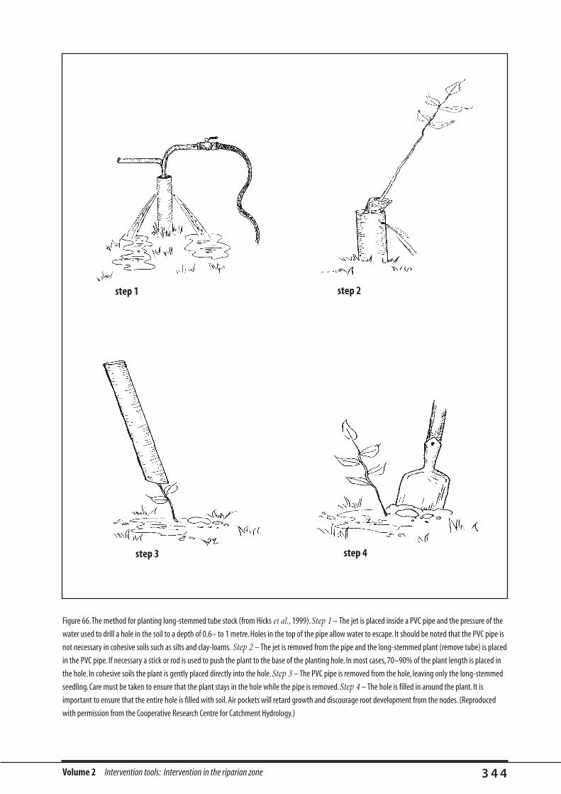
Volume 2 Intervention tools: Intervention in the riparian zone 3 4 4
Figure 66.The method for planting long-stemmed tube stock (from Hicks et al., 1999).Step 1 – The jet is placed inside a PVC pipe and the pressure of the
water used to drill a hole in the soil to a depth of 0.6– to 1 metre. Holes in the top of the pipe allow water to escape. It should be noted that the PVC pipe is
not necessary in cohesive soils such as silts and clay-loams. Step 2 – The jet is removed from the pipe and the long-stemmed plant (remove tube) is placed
in the PVC pipe. If necessary a stick or rod is used to push the plant to the base of the planting hole. In most cases, 70–90% of the plant length is placed in
the hole. In cohesive soils the plant is gently placed directly into the hole.Step 3 – The PVC pipe is removed from the hole, leaving only the long-stemmed
seedling. Care must be taken to ensure that the plant stays in the hole while the pipe is removed.Step 4 – The hole is filled in around the plant. It is
important to ensure that the entire hole is filled with soil. Air pockets will retard growth and discourage root development from the nodes. (Reproduced
with permission from the Cooperative Research Centre for Catchment Hydrology.)
step 1 step 2
step 3 step 4
Volume 2 Intervention tools: Intervention in the riparian zone 3 4 5
By Jim Burston* and Wayne Brown†
The factors for success in direct seeding are:
• site preparation;
• time of sowing;
• seed viability/species selection; and
• maintenance of the site.
The broad principles of direct seeding have been the topic
of a number of books (Dalton, 1993,Venning 1988), a
national conference (Greening Australia Ltd, 1990) and
other extension material.
4.1. What are the advantages of direct seedingcompared to tubestock?
1. Plant density: an average germination, using a seed
mix of 1 kg/ha, will deliver approximately 4,000–6,000
seedlings/ha (Dalton, 1993; M. Campbell, pers.
comm.). Compare this to tubestock, using a 3 m by 3 m
spacing, which produces less fewer than 1,000
seedlings/ha.
2. Cost: site preparation and fencing costs are the same
for either technique. However, direct seeding will
require approximately 1 kg of seed mix (approximate
price of $170/kg), whereas tube stock at $0.50 per
seedling (@ 1,000/ha) will cost $500.
3. Species diversity: most sites in South Australia are
sowing, on average, 20–25 species and at some sites the
range is 35–45. This level of diversity is not feasible
using tubestock plantings.
4. Randomness: most tubestock planting tends to be done
on a rigid adherence to a 3 m by 3 m format. This leads
to a regular, pine-plantation-like appearance quite
unlike the variability of the natural landscape. The
results of direct seeding more closely approximate the
natural landscape.
5. Growth rates: many first-time direct seeders are
disappointed with the early results as compared with
tubestock planting. Although direct-seeded seedlings
might seem to grow more slowly, experience in South
Australia indicates that, by year 2, the height of these
seedlings surpasses that of tubestock. In the ensuing
years the difference in performance widens.
6. Time: for the average site, one hectare (= 3 linear km of
sowing) of direct seeding will take approximately 20
minutes with the mechanical seeder. How long would it
take you to plant 1,000 tubestock trees?
4.2. Site preparation
Undoubtedly the most important factor in a successful
revegetation program based on direct seeding is weed control
(both herbaceous and woody).The vast majority of
revegetation projects fail due to poor weed control.Good
weed control starts with understanding the weed spectrum at
your revegetation site.Depending upon the weed spectrum
(eg.couch, kikuyu, phalaris, cocksfoot, gorse, blackberry)
weed control may need to be initiated up to 24 months before
sowing.This is particularly important if the weed spectrum
includes aggressive summer-growing plants.Good weed
control means a complete kill of all weeds.Weed control
ensures adequate soil moisture for plants to grow through the
summer months.The experience from hundreds of
revegetation sites across South Australia is that, unless weed
control is excellent, direct seeding will fail. In fact, if you don’t
control your weeds, don’t bother with direct seeding.
Control of most herbaceous weeds is generally achieved
through the application of a knockdown herbicide (eg.
glyphosate 360 g/L, @ 1–2 L/ha). For best results, two
applications should be made: the first at 1–2 months
before sowing, and the second 1 week before sowing. Some
broadleaf weeds (eg. strawberry clover, prickly lettuce,
wire-weed) can be controlled with herbicides such as
MCPA®, DiCamba®, and Ally®. Extreme care should be
taken to ensure that no herbicide enters the stream.
Some practitioners have encouraged the use of residual
herbicides to achieve satisfactory weed control. However,
4. Direct-seeding methods
*South Australian Department for Environment, Heritage and Aboriginal Affairs, GPO Box 1047, Adelaide 5001. Ph: (08) 8204 9180, Fax: (08) 8204 9144,
Email: [email protected]
†Mount Lofty Ranges Catchment Program, 5c Cameron Road, Mount Barker, SA 5251.
Volume 2 Intervention tools: Intervention in the riparian zone 3 4 6
unless the soils to which these herbicides are applied have
a high clay content, there is a risk of herbicide leaching
into the zone where the seeds have been laid (and
elsewhere for that matter).
For best growth, it is desirable to remove weed
competition for a distance of 1.5 m from the seedlings.
This will ensure the seedlings have access to sufficient soil
moisture and nutrients. Good weed control will render
fertiliser application unnecessary.
Weed control with herbicides generally takes the form of
blanket, strip or spot spraying. When revegetating
watercourses, it is desirable to allow weeds to grow to a
height of approximately 150 mm before spraying. As the
weeds die, they will form a mulch and protect the soil from
erosion (but not necessarily flood events). Sowing in
spring will also reduce the chance of the site being
damaged by a major flood (in southern Australia) and
severe frosts. On steeper slopes, or where access may be
difficult, strip or spot spraying is appropriate.
Grading and cultivation are two other methods of weed
control. Both techniques have serious pitfalls. They
physically remove the seed bank that is stored in the top
few centimetres of the soil profile, exposing the site to
erosion in heavy rainfall events, and may change the weed
spectrum. Many hard-coated seeds can survive in the soil
for many years (eg. seeds of Acacia spp. may survive up to
120 years). Any potential for natural regeneration from the
seed bank to complement the direct seeding is lost if site
preparation involves grading or cultivation.
4.3. Seed treatment/seed viability/seeding rates
Many individuals tend to be obsessed with seeding rates
and have devised all sorts of formulas to determine the
‘correct’ rate. Our view is that much of this concern is
unwarranted. The most important factor is to ensure that
there is an adequate floristic (ie. wattles, banksias,
bottlebrushes, gum trees, tea-trees etc.) and structural
diversity (ie. trees, shrubs, grasses) within the seed mix. The
approach to revegetation in South Australia has been to
encourage and develop the seed-collecting skills of
landholders. Germination tests are unnecessary if emphasis
is placed on collecting fertile seed, which is an easy task.
Most hard-coated seeds (eg. Acacia spp.) will require some
form of treatment (ie. scarification) before sowing. The
easiest method is to place the seeds in very hot water for a
short time; for further details see Bonney (no date). This
can be done a few days before sowing.
4.4. Sow at the right time
Sowing should be timed to coincide with optimal conditions
of soil moisture and temperature. In southern Australia,
where sites receive rainfall of >450 mm pa, the optimal time
is spring (ie.August–October, depending upon average
annual rainfall). In fact, direct seeding is arguably more
successful in years of slightly below average annual rainfall,
due to less opportunity for weed growth. In regions receiving
<450 mm, May–June is generally the preferred time of
sowing (ie. after the break of the season). In particularly dry
years, or where a late break to the season is encountered, it
may not be possible to undertake direct seeding.
4.5. Methods of direct seeding
The depth to which seeds are sown will have a major
bearing on the success of direct seeding. It is important
that seed has good contact with the soil. Ideal burial depth
can vary according to the amount of light required by the
seed. A general rule of thumb is to sow seed at a depth that
is twice its diameter (Dalton, 1993).
Most direct seeding is done using machines that resemble
up-market ‘1080’ rabbit-bait layers. This simple ‘farmer
friendly’ technology is central to the widespread adoption
of direct seeding in South Australia.
All direct-seeding machinery currently used in South
Australia performs the following tasks:
• removal of soil and trash (ie. generally the top 1–2 cm
of the soil profile);
• preparation of a level seedbed for sowing with standard
(or modified) agricultural seedling implements;
• ensuring that germination takes place in mineral soil; and
• pressing the seed into the soil in order to minimise
consumption by ants (Dalton, 1993).
Where access is limited, machines can be attached to 4WD
motorbikes. Where access can be achieved only on foot,
hand seeding is the answer. The procedures for hand
seeding are outlined in Figure 67.
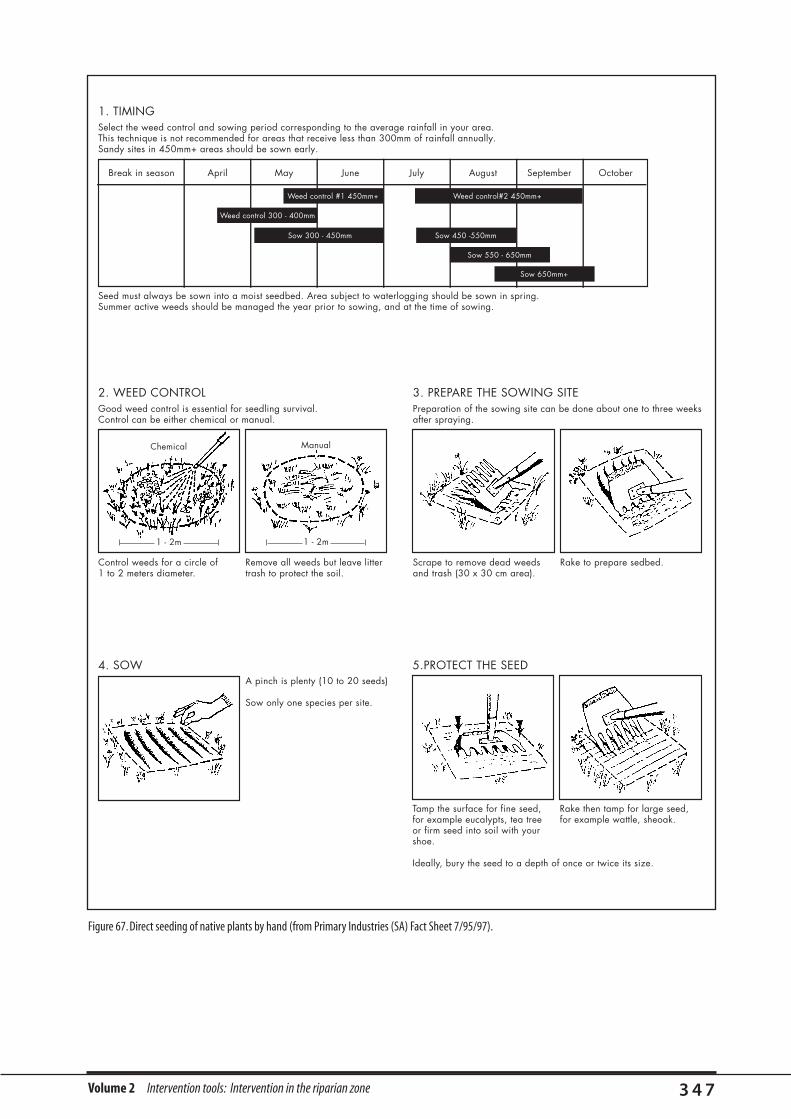
Volume 2 Intervention tools: Intervention in the riparian zone 3 4 7
Figure 67. Direct seeding of native plants by hand (from Primary Industries (SA) Fact Sheet 7/95/97).
2. WEED CONTROL
Control weeds for a circle of 1 to 2 meters diameter.
Good weed control is essential for seedling survival.Control can be either chemical or manual.
ManualChemical
1 - 2m1 - 2m
Remove all weeds but leave littertrash to protect the soil.
4. SOW 5.PROTECT THE SEED
Tamp the surface for fine seed,for example eucalypts, tea treeor firm seed into soil with yourshoe.
Ideally, bury the seed to a depth of once or twice its size.
Rake then tamp for large seed, for example wattle, sheoak.
3. PREPARE THE SOWING SITE
Scrape to remove dead weedsand trash (30 x 30 cm area).
Preparation of the sowing site can be done about one to three weeksafter spraying.
Rake to prepare sedbed.
A pinch is plenty (10 to 20 seeds)
Sow only one species per site.
1. TIMING
Seed must always be sown into a moist seedbed. Area subject to waterlogging should be sown in spring.Summer active weeds should be managed the year prior to sowing, and at the time of sowing.
Break in season April May June July August September October
Select the weed control and sowing period corresponding to the average rainfall in your area.This technique is not recommended for areas that receive less than 300mm of rainfall annually.Sandy sites in 450mm+ areas should be sown early.
Weed control #1 450mm+
Sow 450 -550mm
Sow 550 - 650mm
Sow 650mm+
Weed control 300 - 400mm
Sow 300 - 450mm
Weed control#2 450mm+
Volume 2 Intervention tools: Intervention in the riparian zone 3 4 8
In the agricultural regions of South Australia, there are
only two soil types which present problems for direct
seeding: alkaline, black, cracking clays (these sites were
originally native grasslands); and deep, non-wetting sands
in low rainfall areas (ie. less than 350 mm pa).
In the past two years, the success rate of direct seeding
onto non-wetting sands has been dramatically improved
with the use of wetting agents at the time of sowing, seed
treatment before sowing and advances in seeding
machinery. Successful germination on cracking clay has
been achieved, but most seedlings die as the soil cracks
upon drying.
4.6. Use of local species
For the past decade there has been a concerted effort to
use indigenous species for revegetation. The reasons are
many, including:
• maintaining landscape character;
• conserving biodiversity;
• avoiding genetic pollution of remnant vegetation; and
• longevity of local species.
South Australia is littered with sites that have been planted
with ‘exotic’ native species (ie. Australian species that are
not indigenous to that area). Unsurprisingly, most of these
sites have failed in the longer term (ie. 15–20 years) and
now require a second revegetation effort. Species selection
can vary within a few hundred metres, owing to a change
in aspect, soil type, geology or any number of other
factors. Thus, species lists have to be very site specific.
In South Australia, several landholders (including the
author) have planted river oak (Casuarina
cunninghamiana) along their watercourses. We do not
recommend this species because it appears to have a habit
similar to willows: its roots protrude into the channel,
thereby reducing its capacity. This is of particular concern
on the smaller watercourses (ie. < 4th order).
4.7. Maintenance
Young seedlings are vulnerable to defoliation from pests
such as red-legged earth mite and lucerne flea. In some
circumstances, it may be necessary to add an insecticide
(eg. Le Mat®) to the herbicide solution. It is essential that
extreme caution be exercised when applying insecticides
near watercourses, regardless of the concentration.
It is highly desirable to provide young plants the
opportunity to grow through a second summer in a weed-
free environment. This can be achieved by spraying the
site with a knockdown herbicide, at a reduced rate (ie.
glyphosate 360 g/L @ 0.5 L/ ha), during late winter (ie. late
July–early August). This approach may cause minor tip-
burning to some species, but it is quite safe. At this time,
the young native plants are relatively dormant as
compared with introduced grasses and broadleaf weeds.
Most native plants will be physically shielded from the
herbicide by the growth of herbaceous weeds.
Some individuals may become concerned that direct
seeding can create a situation of ‘too many seedlings’, and
express a desire to ‘thin-out’ the site. Over time, nature will
ensure self-thinning, leaving only the strongest
individuals.
4.8. Conclusion
River engineers build erosion control structures mindful
of the fact that vegetation is a vital tool in attaining a
stable watercourse. However, the revegetation component
is the weak link in the chain. Most revegetation is
undertaken using an outdated technology — tubestock
planting. There has been nearly a decade of successful use
of direct seeding for broad-acre revegetation. The
technique is dependent upon good weed control, sowing at
the right time and using viable seed. Most importantly, the
method is cheap and farmer friendly.
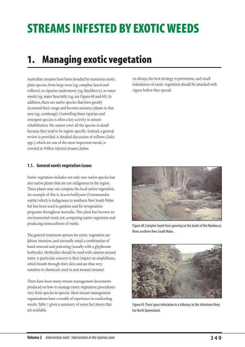
Volume 2 Intervention tools: Intervention in the riparian zone 3 4 9
STREAMS INFESTED BY EXOTIC WEEDS
Australian streams have been invaded by numerous exotic
plant species, from large trees (eg. camphor laurel and
willows), to riparian understorey (eg. blackberry), to water
weeds (eg. water hyacinth) (eg. see Figure 68 and 69). In
addition, there are native species that have greatly
increased their range and become nuisance plants in that
area (eg. cumbungi). Controlling these riparian and
emergent species is often a key activity in stream
rehabilitation. We cannot cover all the species in detail
because they tend to be region-specific. Instead, a general
review is provided. A detailed discussion of willows (Salix
spp.), which are one of the most important weeds, is
covered in Willow infested streams, below.
1.1. General exotic vegetation issues
Exotic vegetation includes not only non-native species but
also native plants that are not indigenous to the region.
These plants may out-compete the local native vegetation.
An example of this is Acacia bailleyana (Cootamundra
wattle) which is indigenous to southern New South Wales
but has been used in gardens and for revegetation
programs throughout Australia. This plant has become an
environmental weed, out-competing native vegetation and
producing monocultures of wattle.
The general treatment options for exotic vegetation are
labour intensive, and normally entail a combination of
hand removal and poisoning (usually with a glyphosate
herbicide). Herbicides should be used with caution around
water. A particular concern is their impact on amphibians,
which breath through their skin and are thus very
sensitive to chemicals used in and around streams!
There have been many stream management documents
produced on how to manage exotic vegetation; procedures
vary from species to species. Most stream management
organisations have a wealth of experience in eradicating
weeds. Table 1 gives a summary of some fact sheets that
are available.
As always, the best strategy is prevention, and small
infestations of exotic vegetation should be attacked with
vigour before they spread.
1. Managing exotic vegetation
Figure 68. Camphor laurel trees growing on the banks of the Nambucca
River, northern New South Wales.
Figure 69.‘Parra’ grass infestation in a tributary to the Johnstone River,
Far North Queensland.

Volume 2 Intervention tools: Intervention in the riparian zone 3 5 0
Table 1. Common riparian weed species across Australia, and where you can get information on how to control them. (for full references see Bibliography of
technical information; Miscellaneous planning tools, this Volume).
Plant(s) Title of publication Contact organisation Description
Gorse, blackberry, briar rose and Woody Weed Control along SA DENR1
any other woody weeds Water Courses
Common bullrush Control of Cumbungi Qld DNR2 Emergent native which grows up to 4 m in still or
(two species—narrow-leafed cumbungi slow-flowing water up to 2 m deep.
(Typha domingensis), and broad-leafed The plant has a strong and extensive root system
cumbungi (Typha orientalis) and is very useful for erosion control and as
habitat for waterbirds and amphibians, but in
isolated situations it can congest streams
(particularly an issue in irrigation systems),
restricting flow and trapping sediment. Typha
should only be removed where it is having an
unacceptable impact on the hydraulic conditions
of the stream.
Water hyacinth (Eichhornia crassipes) Control of Water Hyacinth: Qld DNR Free-floating aquatic plant found in still or slow-
the worst aquatic weed in the world flowing water.The weed is extremely quick to
choke watercourses, and reduce oxygen and light
levels in the stream.
Salvinia (Salvinia molesta) Control of Salvinia Qld DNR Floating aquatic fern (from Brazil) found in still or
slow-flowing water. Grows into dense mats,
choking streams and reducing the oxygen and
light levels in the stream.
Cats claw creeper (Macfadyena unguis-cati) Control of Exotic Vines Qld DNR Found in northern NSW and southern Qld.
Madeira vine (Anredera cordifolia)
Willows, ash and poplars Exotic Trees along Watercourses SA DENR Large exotic trees, can infest streams.
Mount Lofty
Ranges
Catchment
Program
Camphor laurel (Cinnamomum camphora) Camphor Laurel Control B Hungerford , Large exotic trees that that are prolific in coastal
NSW regions of northern NSW and southern Qld.
DLWC:
(unpublished)
Available through
Murwillumbah
district office
of DLWC
2. Management of exotic weeds
1SA DENR = South Australian Department of Environmental and Natural Resources
2Qld DNR = Queensland Department of Natural Resources
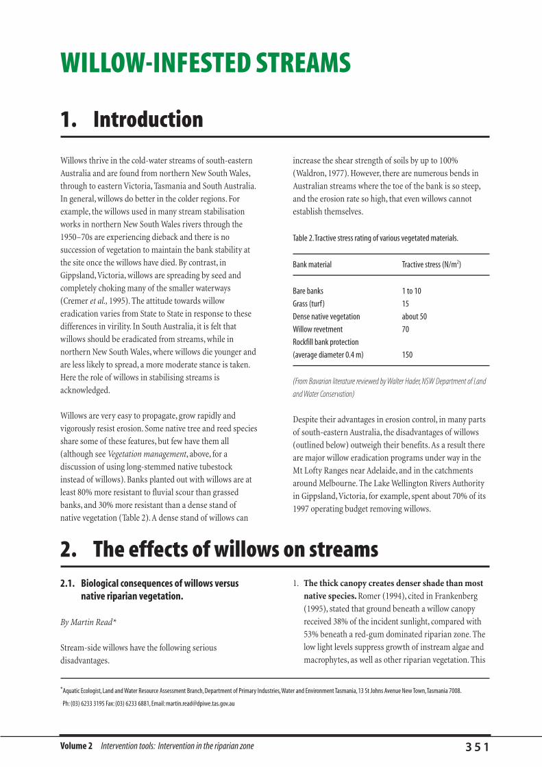
Volume 2 Intervention tools: Intervention in the riparian zone 3 5 1
WILLOW-INFESTED STREAMS
Willows thrive in the cold-water streams of south-eastern
Australia and are found from northern New South Wales,
through to eastern Victoria, Tasmania and South Australia.
In general, willows do better in the colder regions. For
example, the willows used in many stream stabilisation
works in northern New South Wales rivers through the
1950–70s are experiencing dieback and there is no
succession of vegetation to maintain the bank stability at
the site once the willows have died. By contrast, in
Gippsland,Victoria, willows are spreading by seed and
completely choking many of the smaller waterways
(Cremer et al., 1995). The attitude towards willow
eradication varies from State to State in response to these
differences in virility. In South Australia, it is felt that
willows should be eradicated from streams, while in
northern New South Wales, where willows die younger and
are less likely to spread, a more moderate stance is taken.
Here the role of willows in stabilising streams is
acknowledged.
Willows are very easy to propagate, grow rapidly and
vigorously resist erosion. Some native tree and reed species
share some of these features, but few have them all
(although see Vegetation management, above, for a
discussion of using long-stemmed native tubestock
instead of willows). Banks planted out with willows are at
least 80% more resistant to fluvial scour than grassed
banks, and 30% more resistant than a dense stand of
native vegetation (Table 2). A dense stand of willows can
increase the shear strength of soils by up to 100%
(Waldron, 1977). However, there are numerous bends in
Australian streams where the toe of the bank is so steep,
and the erosion rate so high, that even willows cannot
establish themselves.
Table 2.Tractive stress rating of various vegetated materials.
Bank material Tractive stress (N/m2)
Bare banks 1 to 10
Grass (turf) 15
Dense native vegetation about 50
Willow revetment 70
Rockfill bank protection
(average diameter 0.4 m) 150
(From Bavarian literature reviewed by Walter Hader, NSW Department of Land
and Water Conservation)
Despite their advantages in erosion control, in many parts
of south-eastern Australia, the disadvantages of willows
(outlined below) outweigh their benefits. As a result there
are major willow eradication programs under way in the
Mt Lofty Ranges near Adelaide, and in the catchments
around Melbourne. The Lake Wellington Rivers Authority
in Gippsland,Victoria, for example, spent about 70% of its
1997 operating budget removing willows.
1. Introduction
1. The thick canopy creates denser shade than most
native species. Romer (1994), cited in Frankenberg
(1995), stated that ground beneath a willow canopy
received 38% of the incident sunlight, compared with
53% beneath a red-gum dominated riparian zone. The
low light levels suppress growth of instream algae and
macrophytes, as well as other riparian vegetation. This
*Aquatic Ecologist, Land and Water Resource Assessment Branch, Department of Primary Industries,Water and Environment Tasmania, 13 St Johns Avenue New Town,Tasmania 7008.
Ph: (03) 6233 3195 Fax: (03) 6233 6881, Email: [email protected]
2.1. Biological consequences of willows versusnative riparian vegetation.
By Martin Read*
Stream-side willows have the following serious
disadvantages.
2. The effects of willows on streams
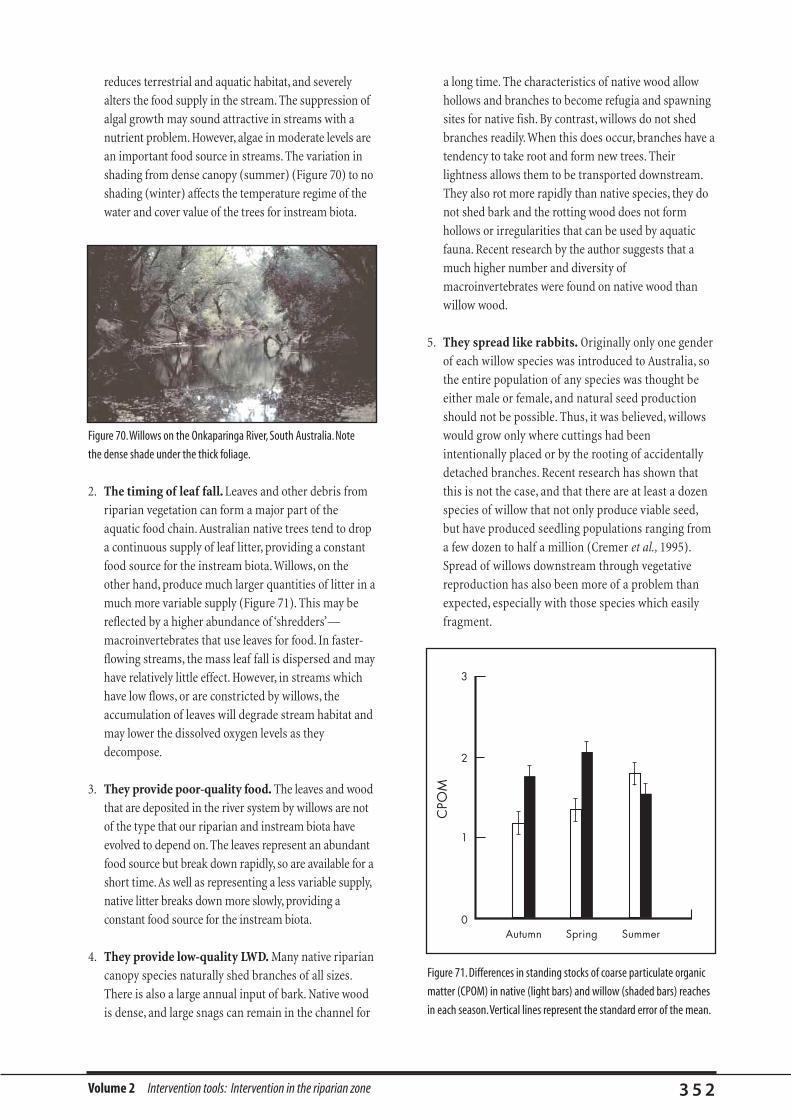
Volume 2 Intervention tools: Intervention in the riparian zone 3 5 2
reduces terrestrial and aquatic habitat, and severely
alters the food supply in the stream. The suppression of
algal growth may sound attractive in streams with a
nutrient problem. However, algae in moderate levels are
an important food source in streams. The variation in
shading from dense canopy (summer) (Figure 70) to no
shading (winter) affects the temperature regime of the
water and cover value of the trees for instream biota.
2. The timing of leaf fall. Leaves and other debris from
riparian vegetation can form a major part of the
aquatic food chain. Australian native trees tend to drop
a continuous supply of leaf litter, providing a constant
food source for the instream biota. Willows, on the
other hand, produce much larger quantities of litter in a
much more variable supply (Figure 71). This may be
reflected by a higher abundance of ‘shredders’—
macroinvertebrates that use leaves for food. In faster-
flowing streams, the mass leaf fall is dispersed and may
have relatively little effect. However, in streams which
have low flows, or are constricted by willows, the
accumulation of leaves will degrade stream habitat and
may lower the dissolved oxygen levels as they
decompose.
3. They provide poor-quality food. The leaves and wood
that are deposited in the river system by willows are not
of the type that our riparian and instream biota have
evolved to depend on. The leaves represent an abundant
food source but break down rapidly, so are available for a
short time.As well as representing a less variable supply,
native litter breaks down more slowly, providing a
constant food source for the instream biota.
4. They provide low-quality LWD. Many native riparian
canopy species naturally shed branches of all sizes.
There is also a large annual input of bark. Native wood
is dense, and large snags can remain in the channel for
a long time. The characteristics of native wood allow
hollows and branches to become refugia and spawning
sites for native fish. By contrast, willows do not shed
branches readily. When this does occur, branches have a
tendency to take root and form new trees. Their
lightness allows them to be transported downstream.
They also rot more rapidly than native species, they do
not shed bark and the rotting wood does not form
hollows or irregularities that can be used by aquatic
fauna. Recent research by the author suggests that a
much higher number and diversity of
macroinvertebrates were found on native wood than
willow wood.
5. They spread like rabbits. Originally only one gender
of each willow species was introduced to Australia, so
the entire population of any species was thought be
either male or female, and natural seed production
should not be possible. Thus, it was believed, willows
would grow only where cuttings had been
intentionally placed or by the rooting of accidentally
detached branches. Recent research has shown that
this is not the case, and that there are at least a dozen
species of willow that not only produce viable seed,
but have produced seedling populations ranging from
a few dozen to half a million (Cremer et al., 1995).
Spread of willows downstream through vegetative
reproduction has also been more of a problem than
expected, especially with those species which easily
fragment.
Figure 70.Willows on the Onkaparinga River, South Australia. Note
the dense shade under the thick foliage.
Figure 71. Differences in standing stocks of coarse particulate organic
matter (CPOM) in native (light bars) and willow (shaded bars) reaches
in each season.Vertical lines represent the standard error of the mean.
CPO
M
Autumn Spring Summer0
1
2
3
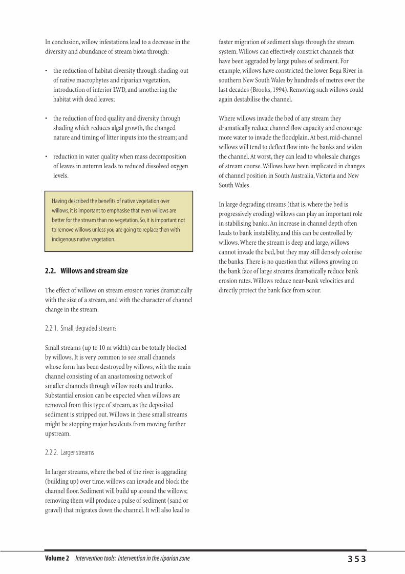
Volume 2 Intervention tools: Intervention in the riparian zone 3 5 3
In conclusion, willow infestations lead to a decrease in the
diversity and abundance of stream biota through:
• the reduction of habitat diversity through shading-out
of native macrophytes and riparian vegetation,
introduction of inferior LWD, and smothering the
habitat with dead leaves;
• the reduction of food quality and diversity through
shading which reduces algal growth, the changed
nature and timing of litter inputs into the stream; and
• reduction in water quality when mass decomposition
of leaves in autumn leads to reduced dissolved oxygen
levels.
2.2. Willows and stream size
The effect of willows on stream erosion varies dramatically
with the size of a stream, and with the character of channel
change in the stream.
2.2.1. Small, degraded streams
Small streams (up to 10 m width) can be totally blocked
by willows. It is very common to see small channels
whose form has been destroyed by willows, with the main
channel consisting of an anastomosing network of
smaller channels through willow roots and trunks.
Substantial erosion can be expected when willows are
removed from this type of stream, as the deposited
sediment is stripped out. Willows in these small streams
might be stopping major headcuts from moving further
upstream.
2.2.2. Larger streams
In larger streams, where the bed of the river is aggrading
(building up) over time, willows can invade and block the
channel floor. Sediment will build up around the willows;
removing them will produce a pulse of sediment (sand or
gravel) that migrates down the channel. It will also lead to
faster migration of sediment slugs through the stream
system. Willows can effectively constrict channels that
have been aggraded by large pulses of sediment. For
example, willows have constricted the lower Bega River in
southern New South Wales by hundreds of metres over the
last decades (Brooks, 1994). Removing such willows could
again destabilise the channel.
Where willows invade the bed of any stream they
dramatically reduce channel flow capacity and encourage
more water to invade the floodplain. At best, mid-channel
willows will tend to deflect flow into the banks and widen
the channel. At worst, they can lead to wholesale changes
of stream course. Willows have been implicated in changes
of channel position in South Australia,Victoria and New
South Wales.
In large degrading streams (that is, where the bed is
progressively eroding) willows can play an important role
in stabilising banks. An increase in channel depth often
leads to bank instability, and this can be controlled by
willows. Where the stream is deep and large, willows
cannot invade the bed, but they may still densely colonise
the banks. There is no question that willows growing on
the bank face of large streams dramatically reduce bank
erosion rates. Willows reduce near-bank velocities and
directly protect the bank face from scour.
Having described the benefits of native vegetation over
willows, it is important to emphasise that even willows are
better for the stream than no vegetation. So, it is important not
to remove willows unless you are going to replace then with
indigenous native vegetation.

Volume 2 Intervention tools: Intervention in the riparian zone 3 5 4
With contributions from David Outhet*, Jim Burston† , Jason
Carter§, and Ross Scott¶.
While willows have great potential in stream stabilisation
works, it is better, wherever possible, to avoid using them.
This policy rests on the golden rule of stream
rehabilitation: "it costs 10 to 100 times more to reverse our
past mistakes than it did to make them". The removal of
willows is a challenging problem due to the vigour of their
growth, and their propensity to grow from limbs or twigs
falling to the ground. The following section illustrates how
some Australian stream managers are tackling the removal
of willows. The removal itself is only part of the plan.
Before any willows are removed, a long-term stream
rehabilitation strategy should be adopted, including a
revegetation technique, stream fencing, and maintenance
review. Successful revegetation after removing willows is
very important. Without it, the removal will most likely
reduce the stability and environmental value of the
stream, rather than improve it.
3.1. When should managers consider leavingwillows?
There are a few situations where willows may substantially
improve the ecological recovery of stream systems, and
improve the long-term stability.
• In a retard field, willows grown between the retards are
very successful at trapping the fine sediment that is
essential for growing native plants. In gravel-bed
streams, without willows or some other vegetation
type, the dominant sediment deposited behind the
retards is gravel or coarse sand. It may be difficult to
trap finer material. Willows tend to be better than
native tree species in trapping this sediment. To an
extent this may be because there has been little work
on using natives in this situation, so it is not yet known
which species are appropriate. When the fine sediment
has accumulated, the willows should be progressively
replaced by natives.
• Willows might be retained on aggressively eroding
outside bends where further erosion would result in the
loss of native riparian vegetation and other assets on
the stream bank. Native vegetation can be planted
behind the willows to progressively replace them.
• Where there are no other trees in the riverine corridor,
existing willows on the banks are better than nothing
for providing shade, windbreaks, biological diversity,
nutrients to the aquatic ecosystem and nesting
sites/cover for birds.
• Willows can protect and conserve ecologically
important stands of remnant native plants from the
erosive power of the river in places where the flow
energy is too high for native plants alone (usually
where the river is degrading due to human impact).
• Willows may be an important part of the natural
heritage of a town or of a reach of rural river (eg. there
is resistance to removing weeping willows along the
upper Murrumbidgee River because the willows are
considered to be part of the cultural landscape).
3. Managing willows
Before any willows are removed, decide (and budget) on how
to revegetate, fence off the stream, and who is going to do the
extensive follow-up maintenance. A controlled number of
willows on a stream bank is better for the stream than no
vegetation at all!
A monoculture of willows on the banks is better than a
grassed and grazed riparian zone.
Willows need to be tightly managed to prevent their
unwanted spread from any location where they have been
retained.Willows are rapacious colonisers.
*Senior River Scientist, NSW Department of Natural Resources, PO Box 3720, Parramatta, NSW 2124. Ph: (02) 9895 7816, Fax: (02) 9895 7867,
Email:[email protected]†SA Department for Environment, Heritage and Aboriginal Affairs, GPO Box 1047,Adelaide, SA 5001. Ph: (08) 8204 9108, Fax: (08) 8304 9144, Email: [email protected]
§ID&A (SA), 10 Galaxy Way,Athelstone, SA 5076. Ph: (08) 8337 1060, Fax: (08) 8337 1244, Email: [email protected]
¶Manager,West Gippsland Catchment Management Authority, Lake Wellington Catchment, Traralgon,Victoria 3844. Ph:(03) 5175 7800, Fax: (03) 5175 7899,
Email:[email protected]

Volume 2 Intervention tools: Intervention in the riparian zone 3 5 5
3.2. Prioritise willow removal efforts
This section is a compilation of contributions from the
above authors.
Willows have so extensively invaded our waterways, that to
maximise the value of removing them we need to prioritise
our actions. Priorities for willow removal are as follows.
1. Very high. Remove or replace all the willows identified
as the species and hybrids that are supplying seed or
large amounts of branches and twigs to the river. This
removes the prime cause of many problems. Most
willow species in New South Wales can produce seed
and branches, but Salix nigra is the worst offender for
seeding, and Salix fragilis is the worst offender for
production of branches and twigs. Note that special
training is needed to identify willow species and
hybrids (general guidance is provided in Cremer et al.
1995). Willow seeds are transported by wind as well as
streamflow, and willows producing seed germinating
on streambanks may be located up to 30 km away
(Cremer et al., 1995).
2. High. Remove willows in river beds and on bars that
are obstructing and diverting flow. This will have
immediate physical benefits.
3. Medium. Replace willows on alluvial banks on
straight reaches of rivers in equilibrium. This will have
no physical benefit, but has a long-term ecosystem
benefit.
4. Low. Replace willows on alluvial banks on all outside
bends and on straight reaches of degrading rivers. This
will be costly and time-consuming, with no physical
benefit and a risk of starting accelerated erosion, but
will have a long-term ecosystem benefit.
3.3. How you manage willows depends on wherethey are
Management of willows depends on the location of the
willows and the behaviour of the river at the site. River
behaviour is determined from a geomorphic analysis of
field, survey and historical information. If you are unable
to recognise the indicators of flow energy level,
equilibrium, aggradation and degradation, consult a river
behaviour specialist.
3.3.1 Removing willows from small streams
Willows are very effective at halting headcuts or knickpoints
in smaller streams (up to, say, 10 m width).Willows can
often be holding several metres of head-cuts in their roots
over a few kilometres of stream. There are many examples
of major erosion following willow removal as these head-
cuts migrate upstream. Removing the willows without
planning for consequent bed erosion would be foolish.
3.3.2 Managing willows in larger streams
The general rule with willows in larger streams appears to
be that they should be removed wherever possible, so long
as removal does not trigger major erosion, and so long as
they will be replaced quickly with native vegetation. It will
take only about 3–4 years for dead willows to rot away in
streams. Native riparian species are ecologically better
than willows, but willows are better than nothing.
3.3.3 Willows on channel beds and bars, and on bedrock banks
Willows in these situations can be completely removed
(roots included) in one operation provided that:
• the trees in the bed are not controlling bed degradation
(if they are preventing degradation, install bed control
structures before willow removal); and
• there are other trees along the stream to provide shade
etc. (if not, establish native plant communities on
adjacent land and wait at least 10 years for them to
mature before removing the willows).
If clearing is to be done on a long length of channel that has
aggraded because of the build-up of sediment around the
willows, the operation should be done in segments of no
more than one kilometre per year. If too much sediment is
released at once, it may choke the river channel downstream
with a sediment slug.Alternatively, the sand and gravel can
be removed from the river at the same time as the willows
and sold to help pay for the cost of the operation.
Rehabilitation of a section of the Fish River at Bathurst, New
South Wales, provides an example of this. Here, the full cost
of the willow removal is covered by the sale of the sand and
gravel that had deposited in the river over many years. Note
that in such schemes supervisors must ensure that the river
bed is not lowered below its pre-aggradation equilibrium
level (see Sand and gravel extraction as a rehabilitation tool,
in Intervention in the channel, this Volume).
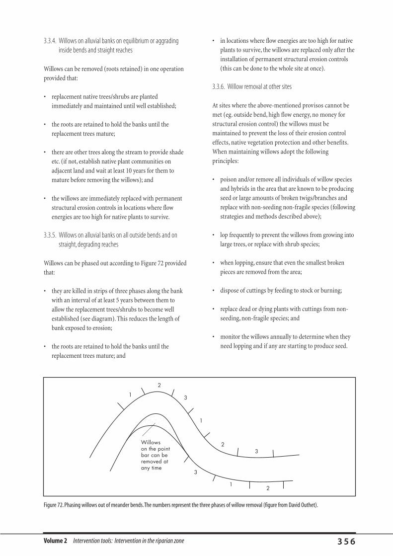
Volume 2 Intervention tools: Intervention in the riparian zone 3 5 6
3.3.4. Willows on alluvial banks on equilibrium or aggradinginside bends and straight reaches
Willows can be removed (roots retained) in one operation
provided that:
• replacement native trees/shrubs are planted
immediately and maintained until well established;
• the roots are retained to hold the banks until the
replacement trees mature;
• there are other trees along the stream to provide shade
etc. (if not, establish native plant communities on
adjacent land and wait at least 10 years for them to
mature before removing the willows); and
• the willows are immediately replaced with permanent
structural erosion controls in locations where flow
energies are too high for native plants to survive.
3.3.5. Willows on alluvial banks on all outside bends and onstraight, degrading reaches
Willows can be phased out according to Figure 72 provided
that:
• they are killed in strips of three phases along the bank
with an interval of at least 5 years between them to
allow the replacement trees/shrubs to become well
established (see diagram). This reduces the length of
bank exposed to erosion;
• the roots are retained to hold the banks until the
replacement trees mature; and
• in locations where flow energies are too high for native
plants to survive, the willows are replaced only after the
installation of permanent structural erosion controls
(this can be done to the whole site at once).
3.3.6. Willow removal at other sites
At sites where the above-mentioned provisos cannot be
met (eg. outside bend, high flow energy, no money for
structural erosion control) the willows must be
maintained to prevent the loss of their erosion control
effects, native vegetation protection and other benefits.
When maintaining willows adopt the following
principles:
• poison and/or remove all individuals of willow species
and hybrids in the area that are known to be producing
seed or large amounts of broken twigs/branches and
replace with non-seeding non-fragile species (following
strategies and methods described above);
• lop frequently to prevent the willows from growing into
large trees, or replace with shrub species;
• when lopping, ensure that even the smallest broken
pieces are removed from the area;
• dispose of cuttings by feeding to stock or burning;
• replace dead or dying plants with cuttings from non-
seeding, non-fragile species; and
• monitor the willows annually to determine when they
need lopping and if any are starting to produce seed.
Figure 72. Phasing willows out of meander bends.The numbers represent the three phases of willow removal (figure from David Outhet).
������������
Willowson the point bar can be removed at any time
1
2
3
1
23
21
3
Volume 2 Intervention tools: Intervention in the riparian zone
3.4. Removing willows
There are four approaches to destroying willows: roots’n’all;
poison and leave; chop and kill; and poison and cut.
3.4.1. Roots’n’all
Willows are removed roots and all, using an excavator. This
is the most extreme method of removal, and is likely to be
the least beneficial to the stream because the substrate is
disturbed as the roots are removed and the protective root
mat is not left in place while native vegetation becomes
established. This method can be used in small, choked
streams where the willows are in the middle of the
channel, causing local flow diversion and channel erosion,
or in bedrock streams where the willow roots are not
stabilising the stream.
3.4.2 Poison and leave
Willows are poisoned by frill cut or stem injection
(Figure 77), the trees are left intact to die and the limbs to
fall and rot of their own accord. This is the cheapest willow
removal method, but the stand of dead timber will be a
safety hazard if the area is accessed by the public. The poor
aesthetic value and rather dramatic vision of a stand of
dead trees is also undesirable in highly visible areas, like
up and downstream of road crossings or in public access
areas. If a number of dead willows fall into the stream at
the same time this may have a dramatic effect on flow
conveyance. So for willow-congested streams that have
nearby land uses sensitive to the effects of flooding, it may
be desirable to remove willow limbs (using either the chop
and poison or kill and cut method) to prevent them
congesting the channel. An example of where the poison-
and-leave technique is being successfully used is the La
Trobe River and streams in north-eastern Victoria. Groups
of willows (say up to 10 trees in a group) are treated by
getting to the sites by boat and stem injecting or frill
cutting the whole group of trees every 12–18 months until
no new shoots are sent out.
3.4.3 Chop and poison
Willow limbs (everything above ground level) are removed
with a chainsaw during the growing season, and the cut
surface is sprayed or painted with poison to kill the roots
and prevent the willow from re-shooting. This type of
removal maintains the roots for erosion control until
replanted vegetation along the stream bank is well enough
established for effective erosion control. This is the most
common method of willow control in Victoria and South
Australia. The main concern with this approach is the
dropping of viable twigs into the stream and onto the
stream bank while lopping the willow. This problem can be
reduced by cutting down the willow during warm, dry
summer periods when the cut material will desiccate and
die, at least on the stream banks.
Willow removal bythe Lake WellingtonRivers Authority,VictoriaThe Lake Wellington Rivers Authority (LWRA) manages the
catchments in the central Gippsland area of south-eastern
Victoria, including the Avon, Macalister,Thomson, and La Trobe
rivers (and tributaries) which discharge into Lake Wellington
(the westernmost of the Gippsland lakes).Many of the streams
within this catchment are either choked with willows, or possess
reaches which have a willow monoculture; other streams have
pockets of willows between native riparian vegetation.
Choked and willow-lined streams
Willows are removed from choked and willow-lined streams
using the cut and kill method.The following procedure was
adopted by LWRA in1996.
1. Willows are cut at ground level by highly skilled chainsaw
operators (the multiple trunks of willows make working
with a chainsaw a hazardous business).
2. The willow stumps are painted with neat ‘Roundup Bi-
Active’ within 20 seconds of cutting.
3. An excavator with a ‘thumb’ attachment is used to lift
willows out of the stream and stockpile them (Figure 73).
4.The stream bank is ‘stick picked’ to remove any twigs or
branches that can germinate.
5. Currently, the stockpiles are burnt but alternative uses for the
timber are being investigated.
6. A reconnaissance visit to the site is planned for 12–18
months after initial removal to poison any new willow growth.
3 5 7

3.4.4. Kill and cut
The willows are poisoned by frill cut or stem injection and
the limbs are cut down once the tree is dead. This
approach has a distinct advantage over the cut and poison
method because it limits the potential for spread of viable
twigs during the lopping process in that only dead willow
is handled, but removal of the dead wood may be
dangerous because of its brittleness. A thick stand of
willows may be a mass of intertwined branches which
makes lopping even green timber dangerous. With some
species of willow the increase in danger while lopping
dead, brittle timber will be an unacceptable risk.
Another limitation of the kill and cut technique is that it
takes at least two treatments and two growing seasons to
kill the willows, hence revegetation is not started (or
growing is not effective) until the third growing season
after the initial poisoning. It is essential during willow
removal that the soil-stabilising function of the willow
roots overlaps as much as possible with the revegetation of
the bank. If willow roots last only 3–4 years before rotting
away, then the roots of the willows killed in the first year
will last for only about one year after revegetation
commences (Figure 76 compares chop and poison and kill
and cut methods).
YEAR 1
YEAR 2
YEAR 3
Growing season
Growing season
Growing season
Dormant season
Dormant season
Dormant season
Chop and poison method
Kill and cut method
Poison all willowsChop down willows and poison stumps
Poison any regrowthPoison any regrowth
Revegetate banks
Cut down dead willows
Revegetate banks
Volume 2 Intervention tools: Intervention in the riparian zone 3 5 8
The long-term plan for these major willow-removal
exercises is to re-establish valuable riparian corridors, by
eventually fencing out stock and revegetating the area with
native vegetation. Figure 74 shows an example of a willow-
infested stream (Traralgon Creek, near the Loy Yang mine
and power station) which has had the willows removed
(cut and kill method), and native species replanted.
In cases where the willow limbs are removed, they can be
felled with a chainsaw and are best stockpiled using an
excavator with a gripping arm or ‘thumb’ (Figure 75).
Figure 73. A stockpile of willows removed from the banks of the
Latrobe River,Victoria.
Figure 74. Hand-planted seedlings on Traralgon Creek (Victoria)
following willow removal.
Figure 75. Gripping arm or ‘thumb’ attached to bucket used for
willow removal on the La Trobe River,Victoria.Figure 76. Chop and poison and kill and cut methods compared.
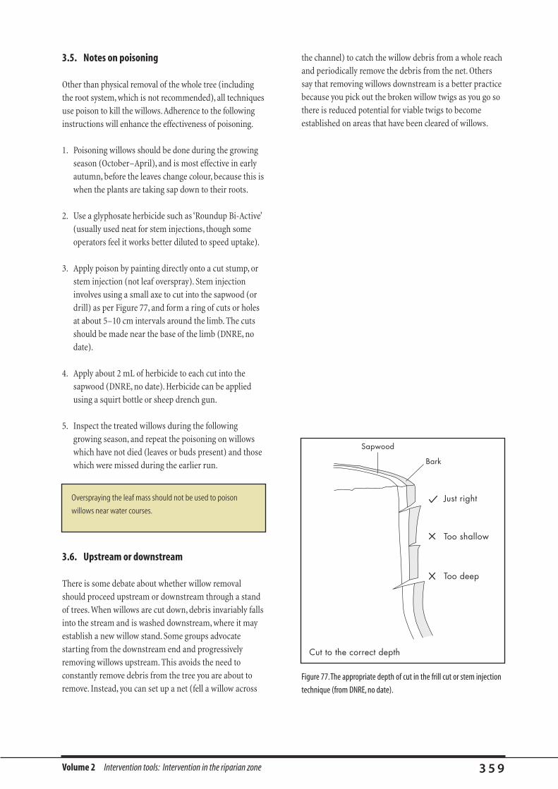
Volume 2 Intervention tools: Intervention in the riparian zone 3 5 9
3.5. Notes on poisoning
Other than physical removal of the whole tree (including
the root system, which is not recommended), all techniques
use poison to kill the willows.Adherence to the following
instructions will enhance the effectiveness of poisoning.
1. Poisoning willows should be done during the growing
season (October–April), and is most effective in early
autumn, before the leaves change colour, because this is
when the plants are taking sap down to their roots.
2. Use a glyphosate herbicide such as ‘Roundup Bi-Active’
(usually used neat for stem injections, though some
operators feel it works better diluted to speed uptake).
3. Apply poison by painting directly onto a cut stump, or
stem injection (not leaf overspray). Stem injection
involves using a small axe to cut into the sapwood (or
drill) as per Figure 77, and form a ring of cuts or holes
at about 5–10 cm intervals around the limb. The cuts
should be made near the base of the limb (DNRE, no
date).
4. Apply about 2 mL of herbicide to each cut into the
sapwood (DNRE, no date). Herbicide can be applied
using a squirt bottle or sheep drench gun.
5. Inspect the treated willows during the following
growing season, and repeat the poisoning on willows
which have not died (leaves or buds present) and those
which were missed during the earlier run.
3.6. Upstream or downstream
There is some debate about whether willow removal
should proceed upstream or downstream through a stand
of trees. When willows are cut down, debris invariably falls
into the stream and is washed downstream, where it may
establish a new willow stand. Some groups advocate
starting from the downstream end and progressively
removing willows upstream. This avoids the need to
constantly remove debris from the tree you are about to
remove. Instead, you can set up a net (fell a willow across
the channel) to catch the willow debris from a whole reach
and periodically remove the debris from the net. Others
say that removing willows downstream is a better practice
because you pick out the broken willow twigs as you go so
there is reduced potential for viable twigs to become
established on areas that have been cleared of willows.
Figure 77.The appropriate depth of cut in the frill cut or stem injection
technique (from DNRE, no date).
Sapwood
Bark
Just right
Too shallow
Too deep
Cut to the correct depth
Overspraying the leaf mass should not be used to poison
willows near water courses.

Volume 2 Intervention tools: Intervention in the riparian zone 3 6 0
Table 2. A comparison of the advantages and disadvantages of conventional and electric fences.
Conventional Electric
Advantages • Relatively little day-to-day maintenance. • Inexpensive to construct and repair.
• Not reliant on external power source. • Quick to construct and repair.
• Still function when overgrown. • Particularly useful for flood gates.
• Familiar to most people. • Curves do not need corner assemblies.
• Long materials life. • Variety of options available for permanent and ‘wash away’
flood gates.
• Animals can escape from fire and flood.
• Gates can be inexpensive and simple.
Disadvantages • Can be costly to purchase materials. • Requires regular checking to ensure proper function.
• Labour-intensive to install. • Electric supply must be available (mains, battery or solar).
• Time-consuming to repair.
In developing this manual, catchment managers from
around the country were canvassed for their views on
information requirements in stream rehabilitation. Many
of the responses highlighted the local problems of erosion
through streamside degradation. For example, Steve
Gallagher (Catchment coordinator, Pitt Water Catchment
Strategy, Clarence, Tasmania) said he needed to know
"how to best fence off streamside vegetation in flood
prone areas. While electric fences are mobile, even these
get washed away during floods". Catherine Travers,
(Border Rivers Catchment Coordinating Committee,
Goondiwindi, Queensland), said she required information
MANAGING STOCK ACCESS TO STREAMS
on "combined management requirements for fencing of
riparian zones".
Stock control through fencing is the most direct and
effective method of riparian zone protection. There are
many different types of fencing available. The two basic
options are conventional and electric fencing, which are
compared in Tables 2 and 3. Alternative designs for flood
gates, and cheap gates for electric fences, are well covered
in manufacturers’ brochures and publications such as
Nicholas and Mack (1996) and Tungkillo and Harrogate
Landcare Groups (no date).
1. Fencing the riparian corridor
Table 3. A comparison of the cost per kilometre of fence for conventional and electric fences (compiled from Nicholas and Mack, 1996; and Tungkillo and
Harrogate Landcare Groups, no date).
CONVENTIONAL ELECTRIC
1) Star picket and 2) Star picket and 3) Wooden post and 4) Permanent, 5-strand3
5-strand barb1 5-strand plain1 ringlock2
Item $ / item No/km $ No/km $ No/km $ $/item No/km $
Strainers 19 5 95 5 95 5 95 21.25 2 42.50
Stays 11 8 88 8 88 8 88 13.80 4 55.2
Droppers 2 100 200 100 200 136 200 2.35 75 176.25
Star pickets 4.20 96 403.2 96 403.2 – – – – –
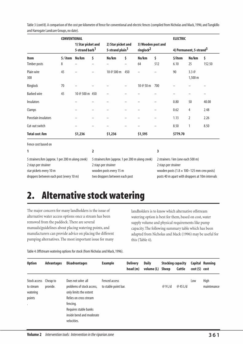
Volume 2 Intervention tools: Intervention in the riparian zone 3 6 1
Table 4. Offstream watering options for stock (from Nicholas and Mack, 1996).
Option Advantages Disadvantages Example Delivery Daily Stocking capacity Capital Running
head (m) volume (L) Sheep Cattle cost ($) cost
Stock access Cheap to Does not solve all Fenced access Low High
to stream provide. problems of stock access, to stable point bar. @ 9 L/d @ 45 L/d maintenance
watering only limits the extent
points Relies on cross stream
. fencing.
Requires stable banks
inside bend and moderate
velocities.
The major concern for many landholders is the issue of
alternative water access options once a stream has been
removed from the paddock. There are several
manuals/guidelines about placing watering points, and
manufacturers can provide advice on placing the different
pumping alternatives. The most important issue for many
landholders is to know which alternative offstream
watering option is best for them, based on cost, water
supply volume and physical requirements like pump
capacity. The following summary table which has been
adapted from Nicholas and Mack (1996) may be useful for
this (Table 4).
2. Alternative stock watering
Table 3 (cont’d). A comparison of the cost per kilometre of fence for conventional and electric fences (compiled from Nicholas and Mack, 1996; and Tungkillo
and Harrogate Landcare Groups, no date).
CONVENTIONAL ELECTRIC
1) Star picket and 2) Star picket and 3) Wooden post and
5-strand barb1 5-strand plain1 ringlock2 4) Permanent, 5-strand3
Item $ / item No/km $ No/km $ No/km $ $/item No/km $
Timber posts 8 – – – – 64 512 6.10 25 152.50
Plain wire 45 – – 10 @ 500 m 450 – – 90 3.3 @
300 1,500 m
Ringlock 70 – – – – 10 @ 50 m 700 – – –
Barbed wire 45 10 @ 500 m 450 – – – – – – –
Insulators – – – – – – 0.80 50 40.00
Clamps – – – – – – 0.62 4 2.48
Porcelain insulators – – – – – – 1.13 2 2.26
Cut-out switch – – – – – – 8.50 1 8.50
Total cost /km $1,236 $1,236 $1,595 $779.70
Fence cost based on
1 2 3
5 strainers/km (approx. 1 per 200 m along creek) 5 strainers/km (approx. 1 per 200 m along creek) 2 strainers / km (one each 500 m)
2 stays per strainer 2 stays per strainer 2 stays per strainer
star pickets every 10 m wooden posts every 15 m wooden posts (1.8 ´ 100–125 mm creo posts)
droppers between each post (every 10 m) two droppers between each post posts 40 m apart with droppers at 10m intervals

Volume 2 Intervention tools: Intervention in the riparian zone 3 6 2
Option Advantages Disadvantages Example Delivery Daily Stocking capacity Capital Running
head (m) volume (L) Sheep Cattle cost ($) cost
Electric Can operate Requires access to 1,100 watt 20 9,000 1,000 200 400 Mains
pump from time, mains power. 240 V L/hr power
pressure or centrifuge. cost.
float switch.
Low Ongoing operational
maintenance. costs.
Quiet.
Low capital cost.
Easy access to
sales and service.
Petrol or Can be installed Usually requires 5HP 20 23,400 2,600 520 500 Fuel, plus
diesel pump virtually manual starting. petrol high
anywhere. Ongoing fuel costs. centrifugal. engine
Ongoing engine maintenance.
maintenance costs.
Solar pump Versatile. High capital costs. 2 panel 20 450 50 10 1,750 Low
Low Requires clear access floating maintenance.
maintenance to sun. solar pump.
Self starting . 2 panel solar 20 24,00 267 53 3,300 Low
No running costs. helical rotor. maintenance.
Best output 4 panel 20 9,000 1,000 200 6,840 Low
during summer tracking solar maintenance.
when water is helical rotor.
required.
Nose pump Cheap to run. Suitable for small stock Nose pump. 5 1,000 111 22 450 Low
Delivers only numbers only. maintenance.
water required
by stock.
Air Allows low-cost May require long runs Air 20 9,000 1,000 200 4,000 Electricity
displacement use of mains of air or electric lines. displacement. L/hr plus low
pump power up to maintenance.
15 km from Relatively high
mains. capital costs.
Copes with sand.
Self priming,
self starting.
Can operate as an
automatic
pressure pump.
Operates efficiently
over a wide range
of volumes.
Table 4 (cont’d). Offstream watering options for stock (from Nicholas and Mack, 1996).

Volume 2 Intervention tools: Intervention in the riparian zone 3 6 3
Option Advantages Disadvantages Example Delivery Daily Stocking capacity Capital Running
head (m) volume (L) Sheep Cattle cost ($) cost
Water ram No running costs. Requires flowing water. Glockemann 20 2,200 244 49 1,350 Low
pump Can operate 110 (1.4 m drop maintenance.
continuously. 1.2 L/s).
Few moving parts.
New designs can
use very low
creek flows and
heads.
Glockemann 20 4,130 459 92 1,750 Low
220 (0.8 m drop, maintenance.
3.5 L/s).
Wind pump No running costs. Requires reliable 8 ft diameter 25 1,200 133 27 3,600 Low
winds or alternative windmill. maintenance.
backup.
Table 4 (cont’d). Offstream watering options for stock (from Nicholas and Mack, 1996).

Volume 2 Glossary 3 6 4
GLOSSARY
Please note: This is not an exhaustive glossary of technical terms used in this manual. There are many cases where a word is
defined the first, and only time that it is used. Thus, we have endeavoured to provide definitions for words that are used several
times in the text. (Some definitions here were modified from the Index of Stream Condition glossary provided by Lindsay
White.)
Where a word is bold it means that it is defined elsewhere in the Glossary. Also note that SRM is an abbreviation for Stream
Rehabilitation Manual and shorthand for A Rehabilitation Manual for Australian Streams,Volume 2, ie. this Volume.
Term Definition
Aesthetic change Has a stream become more or less attractive over time?
Aesthetics Defined in the SRM as how attractive a stream looks to people.
Afflux The increase in water surface elevation above an obstruction in a stream (a measure of
the backwater influence of an obstruction)
Aggradation A progressive build-up of the channel floor with sediment over several years.
Distinguished from the rise and fall of the stream bed during a single flood which is
called scour and deposition.
Algae ‘Plant-like’ organisms that use various chlorophyll compounds to convert sunlight and
instream nutrients into energy stores. This group includes many of the algae that
contribute to the thin layer of slime (periphyton) often found on rocks (predominantly
diatoms), as well as the macroalgae which grow in long strands.
Amplitude The width of a meander belt.
Anabranch A secondary channel of a stream that leaves and then rejoins the trunk stream. The two
channels are separated by stable, vegetated islands that divide flow at discharges nearly
to bankfull.
Anastomosing Multiple branching stream channel (strictly, anastomosing is a subset of anabranching
streams restricted to fine-grained, low-gradient, organic rich systems).
ARI Average recurrence interval (or return period) is the average length of time between
two floods of a given size or larger.
Armour A coarse layer of gravel overlaying finer material on a stream bed.
Armouring Development of a coarse layer of gravel over finer sediments on a stream bed.
Artificial barrier An unnatural obstacle in a stream (eg. a dam wall, weir, culvert) that affects (halts or
delays) fish migration.
Assets Some features that are of value. These can be human assets such as bridges or land, or
they can be natural assets such as organisms. See natural assets.
Volume 2 Glossary 3 6 5
Attraction flow The flow in a fishway that serves to attract fish to the entrance of the fishway.
AUSRIVAS An evaluation package which gives an indication of stream condition by comparing the
observed aquatic macroinvertebrate taxa at a site to the taxa that were predicted to
occur at the site in the absence of environmental stress.
Average The number found by dividing the sum of all the quantities by the number of the
quantities.
Avulsion Sudden abandonment of one channel of a river on a floodplain for a new channel.
BACI design Describes a type of experimental design standing for
Before–After–Calibration–Intervention.
Backwater This is the pool of slower water that develops upstream of a any flow obstruction, eg. a
piece of LWD, or a dam.
Bacteria Single-celled organisms that are associated with the decay of organic matter.
Bag limits The number of fish a recreational fisherman is allowed to take from a stream and keep.
Bank The relatively steep part of a stream channel cross-section, generally considered as being
above the usual water level.
Bankfull The junction between the floodplain and the channel. This point is often difficult to
define in the field, especially where there are benches in the channel.
Bar A local depositional feature within a stream channel. The most common types are mid-
channel bars that form within the channel and point-bars that form on the inside of
bends of meandering streams.
Base level The lowest point to which a stream runs. These can be local base levels (such as a small
lake), or the final base level, the sea.
Basin In Australia, usually refers to a large catchment made up of several catchments that are
large in their own right. For example, the Murray–Darling Basin.
Basket-case reach A stream reach that is in very poor condition. Often the lowest priority for
rehabilitation.
Batter The slope of a bank. Often used to describe changing the bank slope.
Bed stability Bed stability is when the average elevation of the stream bed does not change much
through time. Aggradation or degradation are the two forms of bed instability.
Bedforms Dunes and other shapes moulded in the bed of the river, usually in sand.
Bedload The portion of the sediment load that moves along the floor of the channel.
Benches Flat deposits of sediment that accumulate along streams, above the average water level,
but below the bankfull point.
Volume 2 Glossary 3 6 6
Bend apex The point of a meander bend that has the most curvature. The head of a bend.
Billabong A section of cutoff stream channel (eg. an oxbow lake) usually on a floodplain. The
cutoff channel will progressively fill with sediment over time. Most are only connected to
the river during floods. Adjacent to a lowland reach that is typically filled with water and
only connected laterally to the river when flooding occurs.
Biodiversity A word used to describe biological heterogeneity. It covers the number of species of
plants and animals present, as well as how different they are from one another.
Bio-engineering Incorporating vegetation into engineering structures (eg. willows into bank rip-rap).
Biofilm The mixture of benthic algae, bacteria and fungi which forms a film on submerged
surfaces. This layer is the food source for many macroinvertebrates. Also known as
periphyton.
Bio-indicators Using the health or diversity of organisms in a stream as a measure of the health of the
stream (especially in relation to pollution).
Biological monitoring The monitoring of organisms.
Biomass A measure of the weight of a selected group of organisms (eg. algal biomass,
macroinvertebrate biomass) usually expressed as weight per square metre of streambed.
Biota Plants and animals.
Buffer strips (see buffer-zone)
Buffer-zone Usually refers to a strip of riparian vegetation that separates a stream from a potentially
damaging land use.
Catchment The area of land drained by a river and its tributaries.
Catchment management Actions to manage the human impact on a catchment with the intention of protecting
the natural values of the catchment, whilst protecting its productive potential.
Chain-of-ponds A type of natural stream morphology once common in humid Australia, but now largely
destroyed. Characterised by prominent ponds separated by densely vegetated zones.
Channelisation Engineering actions designed to increase the capacity of a channel to carry flood waters
(typically include desnagging, straightening, and deepening).
Clay Sediment smaller than about 4 microns in diameter.
Clear-water release Release of a flow, usually from a reservoir, that carries less sediment than the water is
capable of transporting. This usually leads to bed and bank erosion.
Clear-water scour The stream channel erosion that is produced by a clear-water release.
Cobbles Gravels larger than about 60 mm in diameter (about the size of a fist).
Volume 2 Glossary 3 6 7
Collectors Animals that collect detrital material for consumption.
Colonisation In biological terms, an expansion in the habitat occupied by organisms by moving into
new areas.
Community An ecological term which collectively describes all the species occurring at a location.
Complexity Structural diversity. A measure of how complicated something is.
Condition State, quality relative to some standard.
Confinement The width of the active floodplain of a stream. Narrow floodplains can be confined by
terraces or rock walls.
Connectivity The physical connection between places. In a stream, refers to connection along a
stream’s length (longitudinal connectivity), and between the stream and its floodplain
(lateral connectivity).
Control (for evaluation) (Evaluation) This is a sampling site or reach which is the same as the rehabilitation site
in every way, except that it is not rehabilitated. The control site is compared with the
rehabilitation site as a way of checking that any changes are a result of the
rehabilitation, rather than some other unconnected event affecting the whole stream.
Control (hydraulic) The point in a stream (such as a constriction or weir) that controls the upstream water
level.
Conveyance The amount of discharge that a stream can carry.
Cover To do with vegetation density, the spread over the ground surface within the streamside
zone when viewed from above. Also to do with instream cover. For biologists, cover can
also mean cover for fish and other animals in a stream.
Crash grazing A short burst of grazing in a protected area.
Created assets In the SRM these are defined as assets that have been created by human disturbance
and should be preserved even though they might not resemble the ‘natural’ condition
(eg. artificially stocked population of a rare fish).
Critical flow Flow with a Froude number of 1.
Culverts Pipes or other structures used to pass water under roads and other crossings.
Cumbungi Otherwise known as bulrush. A common, tall rush in slow moving waters (Typha spp.).
Cutoffs (Meander cutoffs) Where the stream cuts through the neck of a meander bend.
Cyanobacteria A group of photosynthetic bacteria, also known as blue-green algae. Many species are
found in water, and a few produce toxins that can kill ih sufficiently high concentrations.
Decomposers Organisms such as bacteria and fungi which break down organic matter chemically.

Volume 2 Glossary 3 6 8
Degradation Degradation has a broad meaning of reduction in quality, and a specific meaning in
geomorphology of general lowering of a stream bed, usually over a period of years, by
erosional processes.
Degraded assets In the SRM, this has the specific meaning of a natural asset that has been damaged by
human impact so that it no longer has the qualities of the original asset.
Desnagging Removing large woody debris from the bed of streams, to increase conveyance.
Dessication Drying out.
Detritivores Animals that consume detritus.
Detritus Decaying organic matter (predominantly leaves and other vegetable matter).
Direct seeding A method of revegetation where seed is spread directly onto the prepared ground rather
than being germinated in nurseries and grown as tubestock.
Discharge The amount of water flowing in a stream.
Discontinuous gully A gully that is not continuous. Incised sections of gully are separated by zones of
deposition where there is little incision.
Dispersal The movement of animals or plants from their established range into new areas. The
main types of dispersal in streams are drift, aerial dispersal and migration.
Dissolved oxygen Oxygen that is dissolved in water and is therefore available for use by aquatic plants and
animals.
Disturbance A process that pushes a stream or its elements away from an equilibrium state. This can
be a short-lived push (a pulse disturbance) or a more permanent push (a press
disturbance).
Diversity A measure of how varied something is. An ecological community with greater diversity,
will have a large range of species within it.
DLWC The Department of Land and Water Conservation in New South Wales.
Drift A mechanism which allows the downstream migration of organisms. They simply let go
of the substrate and drift with the flow.
Drowned out An obstacle to flow (eg. a weir) is drowned out if the water surface elevation immediately
downstream of the obstacle is approximately equal to the water surface elevation
immediately upstream, and there is no sudden change in the water surface between the
two points.
Dune A bedform formed in sand in the bed of a stream, usually in the order of tens of
centimetres high and long.
Duration The length of time over which something operates. In hydrology, usually refers to the
amount (or percentage) of time that a flow is exceeded.

Volume 2 Glossary 3 6 9
Dynamic equilibrium Oscillations around a gradually changing mean state in a system (eg. a change in the
composition of macroinvertebrate communities as shading reduces water temperature).
Ecology The study of organisms and how they interact with each other and their physical
surroundings.
Ecosystem The sum of everything pertaining to ecology at a location. This includes physical
habitats and organisms.
Effluent The point at which flow leaves one channel to flow in an anabranch.
Electrical conductivity A measure of salinity. The higher the electrical conductivity of a stream the greater the
salinity.
Electrofishing A method of fishing which uses electric currents to stun fish.
Emergent macrophytes Aquatic plants, such as rushes and cumbungi, that are rooted below the water but also
extend above the water.
Environmental flow regime A pattern of flows released from a dam or other regulating structure that are designed to
enhance the environmental condition of a stream given other demands placed on water
from the stream.
EPA Environmental Protection Authority
Ephemeral stream A stream which flows intermittently, ie. it is often dry.
Equilibrium The condition of a stream (whether physical or biological) is stable in relation to the
inputs into the system.
Erosion Modification of the channel boundary by entrainment and removal of sediment.
Estuary The portion of the mouth of a river that is affected by tides (and hence also salinity).
Eutrophication A process which involves the overgrowth of algae and macrophytes in a water body due
to excessive nutrient loads.
Evaluation In the SRM, an assessment of the effectiveness of a strategy. Usually based on
monitoring of some sort, but different from monitoring in that evaluation involves an
assessment of success or failure, not just its description.
Evaluation plan (Evaluation) The detailed plan of how you do your experiment—what you measure,
when, how often etc.
Evolution of habitat Progressive changes in habitat in a natural stream (eg. progressive filling of a cut-off
meander bend).
Execution How the rehabilitation strategy is carried out in practice.
Exotic plants and animals Species of plants or animals that are not naturally found in an area (ie. not indigenous to
the area). Carp, trout and tilapia are examples of exotic fish species, and willows are an
example of an exotic plant. Note that a native Australian species is an exotic when
introduced outside its natural range.

Volume 2 Glossary 3 7 0
Exponential A constantly doubling number sequence (eg. 2,4,8,16….).
Extraction Artificial removal of sand or gravel from a stream.
Failure plane The surface around which mass-failure occurs on a stream bank (often identified by a
tension crack).
Fatal problems Fatal problems in a stream are so severe that they threaten the viability of the
organisms living a stream, eventually leading to extinction. There may be no point
working on other problems until these ones are fixed.
Feasibility An assessment of whether a strategy can really be carried out. See also terminal
unfeasibility.
Feral animals Animals introduced into Australia from another country and declared to be feral by
government (ie. they must be destroyed by law) (eg. foxes, cats, rabbits, carp).
Filamentous algae Algae that grow in long thin strands.
Filter feeders A form of collector, which uses net-like structures to extract passing detrital material
from the stream.
Fish passage The movement of fish around an obstacle.
Flood A flow in a stream that exceeds the normal channel capacity and goes over the banks
onto the floodplain.
Flood frequency How often the stream goes over its banks. Usually expressed as the probability that the
flow will exceed some size in a single year (thus the 1-in-100 year flood would have a 1%
probability of being equalled in any one year. See also ARI and return period.
Flood runner or chute A channel that only flows during floods (may be an anabranch, but it may be smaller).
Floodouts A zone of deposition at the downstream end of a gully or other source of increased
sediment transport.
Floodplain A flat area adjacent to a stream that is covered by floods every year or two. Note the
distinction from a bench (which is flooded much more often) and a terrace (which is
only very rarely flooded).
Flow regime The typical, predictable pattern of flows experienced by a stream over many seasons and
years. The set of flows considered to be responsible for the character of the stream system.
Flow regulation Changes to the timing and volume of flow brought about by dams, diversions or other
interference in a river.
Food web The structure used by ecologists to represent the links between organisms within the
stream. It is based upon the order in which various organisms consume one another.
Frequency How often something occurs.

Volume 2 Glossary 3 7 1
Froude number Ratio of inertial to gravitational forces in a flow. The speed of a small wave on the water
surface relative to the velocity of the water as a whole.
Gabions Baskets of gravel or rocks enclosed by wire used for protecting stream bed and banks.
Gauge A device for continuously measuring the stage of water in a stream.
Gauging structure A structure in a stream that is used to measure the volume of flow. The structure that is
normally found in a stream is a concrete weir or sill.
Geodiversity The number of discrete landform types in a region.
Geographical information system A computer program that manages spatial data in layers. Abbreviated to GIS.
Geomorphology Geomorphology is the study of the Earth’s landforms including their origin and
structure. Fluvial geomorphology is the subset that deals with streams.
GIS See Geographical information system.
Goal The end-point that you are working towards in your rehabilitation. May be defined in
terms of the original condition of a stream.
Grade control structure A structure built in the bed of a stream to limit erosion of the bed. Can be built of rock,
concrete or wood. Operates by reducing velocity, by encouraging vegetation, and by
introducing a hard point in the bed.
Gravel All sediment particles greater than 2 mm in diameter (includes the sub-classes of
granule, pebbles, cobbles and boulders in the Wentworth particle size scale).
Groynes Solid deflection structures in a stream (partial-width structures) that extend to close to
the bank top.
Habitat Loosely defined as a set of physical conditions in which an organism can live.
Head cut Also called a knickpoint. A very steep section of stream bed that migrates upstream if
not held by a bed control. Downstream of a head cut is normally incised and unstable.
Headwaters The most upstream, steepest, portions of a catchment that deliver most water to a
stream system.
Heavy metals Metals with an atomic number greater than 20 (eg. mercury and copper). As pollutants,
they are persistent and can be harmful to a range of aquatic organisms.
Herbaceous weed Any weed that does not develop a woody stem.
Herbivores Animals which consume plant (and algal) material.
Hydraulic geometry A set of power functions that relate changes in the width, flow depth, and velocity of a
channel to changes in discharge.

Volume 2 Glossary 3 7 2
Hydraulic radius The ratio of the cross-sectional area of a channel to the wetted perimeter (ie. the length of
the boundary that is in contact with the water).
Hydraulics The study of the physical effects of the passage of water (as opposed to hydrology which
is concerned with the amount of water moving around).
Hydrology The science that considers the distribution of water over the land (as opposed to
hydraulics that considers the physical effects of the water in its passage).
Impeded recovery Recovery of a stream or its components that is constrained by one or a few press or
pulse disturbances (eg. cattle grazing or point-source pollution).
Incised stream A stream that has eroded its bed and banks such that it has a very low flood frequency.
In other words, the channel cross–sectional area is obviously too large for its catchment
area.
Inflection point The point in a stream bend where one bend ends and the next one begins (often occurs
at a riffle).
Integrity The condition of a system relative to its original condition.
Interstitial spaces The gaps between the particles that make up the stream bed. These spaces are important
habitat for many macroinvertebrates.
Invertebrates Animals without backbones.
Junction The point at which two streams join.
Knickpoint Oversteepened point of erosion in a stream bed. May be a small waterfall. Also called a
headcut.
Large woody debris A dead tree, or portion of a tree, that has fallen into a stream. Usually considered to be
greater than 0.1 m in diameter, and over a metre long. Also called snags or LWD.
Larva A stage in the life cycle of some aquatic invertebrates. Larvae generally do not resemble
the adult form and undergo a pupal stage before becoming an adult.
Larval fish Fish that have just hatched. They are often very different in form to their parents.
Lateral barriers A barrier restricting water and material flow between a stream and its floodplain
(artificial levees would be an example).
Levee A high-point next to a stream bank that is higher than the average height of the
surrounding floodplain. May be formed naturally or artificially.
Life cycle A cycle which links the various forms of an organism from egg to adult.
Limiting problems/variables This is a resource that is required by an organism to survive, but that is most lacking from
/requirements the stream. The limiting requirement limits the ability of a population to recover from
disturbance.

Volume 2 Glossary 3 7 3
Linked problems Problems that are linked so that there is less point fixing one unless you can fix the other.
So, successfully fixing one problem depends on fixing another problem first.
Longitudinal barriers Barriers along a stream’s length that disrupt the movement of water and material (eg.
carbon) along the stream.
Longitudinal continuity A measure of the continuity of the movement of water and material along a stream.
Continuity may be reduced by natural or artificial barriers (eg. willow jams, concrete
dams, diversion channels, pumps).
Lowland reaches Lowlands are broad alluvial or coastal floodplains.
LWD Large woody debris.
Macrocrustaceans Crustaceans such as shrimp and crayfish which are large enough to be seen without a
hand lens.
Macroinvertebrate An invertebrate (animal without a backbone) that is visible to the naked eye.
Macrophyte A water plant. It may be either floating or rooted. Also, see emergent macrophyte.
Manning’s ‘n’ The roughness coefficient in the Manning’s velocity equation. A crude measure of the
resistance to flow in a channel, but is likely to contain all of the uncertainties in a velocity
prediction or measurement.
Mannings equation An empirical equation (ie. based on experiments rather than theory) used to estimate the
velocity, and hence discharge, of a flow.
Mass wasting/failure Gravity failure of a slope (including a stream bank) as a single block.
Median The middle number of a series. If the sequence has an even number of values, the
median is the average of the two middle values.
Megalitre One million litres (divide by 86.4 to convert to cubic metres per second).
Migration (of animals) Recurring long distance travel by an organism. Many fish species migrate up and down
rivers to complete different parts of their life cycle.
Migration (of meander bends) Erosion of the outside (concave) bank of a river such that the river progressively moves
across or down the valley.
Modified catchment A catchment that has been altered by human impact. The most common impacts include
altered land use and flow regime, and the introduction of exotic plants and animals.
Monitoring Gathering information about something in a stream rehabilitation project. May involve
measuring or simply observing change. An essential component of evaluation.
Morphology The shape of something.
Natural Defined here as pre-European condition, including the rates and types of disturbance
that took place.
Volume 2 Glossary 3 7 4
Natural assets Defined in the SRM as features of a stream that are in close to natural (ie. pre-European)
condition. Examples would be an endangered fish species, well preserved riparian
vegetation, or a whole reach that retains many of the original features.
Natural flows The flow that would have existed if present rainfall patterns fell on catchments before
European settlement.
Natural Heritage Trust Money provided for environmental work by the Federal Government following the part-
sale of Telstra. At least tens of millions of dollars are being directed to stream
rehabilitation activities. Also known as NHT.
Nitrogen One of the main nutrients.
Non-point source (or diffuse source). Pollution that is contributed from numerous small sources as opposed
to a single point-source.
Nutrients Chemicals (usually refers to nitrogen and phosphorus) that are essential for plant and
animal growth.
Nymphs A stage in the life cycle of some aquatic insects. Nymphs have a similar form to the adult
insect, but lack wings.
Objectives A clear, measurable statement of what a manager aims to achieve in a project. These are
the specific aims of a rehabilitation project, and are the small steps on the path to
achieving your goals.
Off-channel watering Stock watering point provided away from the stream banks, eg. water may be pumped to
troughs in a paddock.
Organic matter Carbon-based matter of organic origin. This includes vegetable matter as well as the
bodies of dead animals.
Organisms Plants, animals, fungi and bacteria. Things that live.
Overstorey Woody plants greater than 5 m tall, usually with a single stem (eg. eucalypts, banksias,
acacias, and willows).
Parish plans Survey plans made by government of a ‘Parish’ at first settlement, showing the settlement
blocks. An historical source.
Perching (at culverts) A small waterfall formed by a man-made obstruction that forms a barrier to fish
passage.
Perennial flow Flowing all year.
Periphyton A thin layer of algae, bacteria and fungi which grows on stream substrates.
Permanent stream A stream that flows for all of most years.

Volume 2 Glossary 3 7 5
Permeable groynes (More correctly ‘retards’) Groynes constructed of material that allows water to pass
around them (eg. logs, train tracks), as opposed to solid groynes made of rock or
concrete.
pH A measure of the concentration of the acidity or alkalinity of the water (hydrogen ions in
water).
Phosphorus One of the main nutrients.
Phragmites reeds Also known as ‘common reeds’ (Phragmites australis). Occur in slow moving water.
Pilot study A small project designed to check the feasibility of a method or technique before
launching into a major project.
Planform The shape of a stream as seen from the air.
Planktonic algae Algae that float free in the water.
Point bar A sandy deposit on the inside of a meander bend.
Point source A pollution source that can be pinpointed.
Pool The deepest point of a stream bed. Pools usually occur at the outside of stream bends
and may be separated by shallower areas called riffles.
Press disturbance A long-term disturbance.
Problem In the SRM, a ‘problem’ is defined strictly as any process or attribute that threatens a
natural asset or causes it to be damaged, or to no longer be in its natural condition.
Producers Organisms that can use nutrients to generate energy. This includes plants, algae and
bacteria.
Prograde Slowly move into, usually used in the sense of sand gradually moving into a lake or other
water body.
Pulse disturbance A short-lived disturbance.
Q The symbol for discharge.
QDNR Queensland Department of Natural Resources.
Radius of curvature The radius of a circle that fits into a meander bend.
Rating A non-dimensional number for an indicator that is evaluated by converting raw data (eg.
total phosphorus concentrations or observations on site) using a rating table.
Reach A length of stream, typically 5 to 30 km long, which is relatively homogenous with regard
to the hydrology, physical form, water quality and aquatic life.
Volume 2 Glossary 3 7 6
Reach priority categories The nine (9) priority categories that reaches can be assigned to in setting priorities for
stream rehabilitation in the SRM.
Reality check A point in the stream rehabilitation planning procedure when you decide if you should
go back to an earlier step.
Recolonisation The return of a species or community to an area after some form of disturbance.
Recovery Return of a stream system to some state that is considered desirable (usually the natural
state) following disturbance.
Recovery pathway The stages through which a system passes as it gradually recovers.
Regeneration Vegetation that has grown from natural sources of seed or from vegetative growth,
without being artificially planted.
Regime channel A stream channel that is ‘in regime’ neither degrades or aggrades over time.
Region A loose term relating to a tract of country with broadly similar characteristics (eg. the dry
tropics is a region).
Regional conservation value An asset that is rare within a region (as opposed to an asset that is rare within a
catchment but not within a region—which would be classified as having local
conservation value).
Regulated stream Stream flows controlled by releases from a dam, or by some other artificial control.
Rehabilitation The return of as much as possible of the original, pre-European characteristics of a
stream, including the physical structure and stability, water quality, flow regime, and
the suite of organisms in the stream. The organisms present in the stream are a good
measure, in most cases, of the health of the stream, and thus whether it is being
rehabilitated. Ideally, improvements introduced to the stream should be self-sustaining.
Rejuvenation An increase in stream erosion following a fall in the base level. The rejuvenation can
proceed as a ‘wave’ up the tributaries of a stream system.
Remediation Attempts to improve the condition of a stream may produce a stream that is very
different from the natural stream, but nonetheless improved. Remediation is often an
appropriate goal in urban stream rehabilitation.
Replication (Evaluation) This is repeat sampling to identify the inherent variability in the system.
You can have replicates on many scales—replicate rivers to see if the results can be
applied to different streams; replicate study sites within a river to see if all reaches react
in the same way; replicate samples over time, to measure the temporal variability; and
replicate sub-samples within a sample, to measure spatial variability. Thus, when you
sample, you might take 10 samples from the reach instead of one, or 10 samples from
10 streams at the same time.
Volume 2 Glossary 3 7 7
Replication Copying the original state.
Resilience The ability of a community or system to return to equilibrium after a disturbance.
Restoration Replicating the original state of a stream in regard to water quality, structure and
stability, flow regime, and plant and animal communities.
Retards Permeable partial-width structures that only extend to a small percentage of the bank
height.
Return period (of floods) (More correctly ‘average recurrence interval’ or ARI) The average time in years between
two floods of a given size or larger.
Revetment Artificial bank protection, eg. rip-rap.
Riffle The high point in the bed of the stream between two pools (it is often covered in gravel
or coarser material and experiences rapid, turbulent low flows).
Riparian Pertaining to the banks of a river (usually more broadly defined as a strip of land tens of
metres wide along the banks of stream).
Ripples Bedforms that are smaller than dunes (usually centimetres in height).
Root wads The root balls of trees placed in streams. This is usually done by driving the trunk into
the bank.
Roughness A general measure of the hydraulic resistance caused by obstructions to flow (often
measured by the ‘n’ coefficient in the Manning’s equation).
Saline pools Where salt seeps into a deep hole in the stream bed, and it can accumulate in the bottom
of the hole (saline water is denser than freshwater), with salinities often approaching that
of seawater. Saline pools are common in streams in northern and western Victoria.
Salmonids A family of fish from the Northern Hemisphere. This family includes trout and salmon.
There are no native Australian salmonids.
Sample (Evaluation) A measurement of some sort. It could be anything from the average depth
of erosion at a site, as measured by erosion pins, to a measure of water quality, or a
survey of the invertebrate population present at a site.
Sediment slug A wave of sand or gravel that moves down a stream channel (usually introduced into the
stream in a pulse by mining, gullying, major floods or other extreme events).
Scaling A template reach may be found in a different part of the catchment than the target
reach. The dimensions of the template reach that are related to the position of the reach
in the catchment (eg. sediment size, slope, channel size) need to be adjusted to reflect the
dimensions that would be expected in the target reach, given the position and different
condition of the target reach in the catchment (eg. you will probably need to design a
larger channel in a cleared catchment than in a forested one).

Volume 2 Glossary 3 7 8
Scour The short-term erosion of a stream bed (ie. the bed scours and then fills to about the
same level, unless it is degrading or aggrading).
Scour chains Chains inserted vertically into the sand or gravel of a stream bed in order to measure the
amount of scour and fill taking place during a flood.
Scrapers Animals which consume the periphyton which grows on the surface of rocks, plants and
coarser organic matter.
Seasonality (of flows) A difference in flows between seasons of the year.
Secondary circulation A flow velocity across the channel that leads to spiralling currents along the channel. The
circulation is associated with channel bends and is responsible for erosion of meander
bends.
Secondary effects Consequences of a rehabilitation strategy that are not related to the goal or objective of
the strategy. Thus, an increase in flood duration is a secondary effect of adding LWD to a
stream, when the primary effect that was intended was an increase in habitat diversity.
Sediment trap A structure across a stream that creates a backwater in order to trap sediment.
Seeding willows Willows usually reproduce by vegetative growth from cuttings. Some fertile willows can
reproduce by producing seed.
Segment A long portion of stream (consisting of several reaches) that is defined by the general
geological character of the catchment (eg. changes in bedrock, faults, long reaches with
similar slope etc.).
Shear stress The force applied to the bed of a stream by the depth of water (roughly increases with the
depth of water and the slope).
Sheet erosion Erosion of the surface of a paddock or other portion of the catchment as a thin layer of
soil.
Shredders Animals that reduce coarse organic matter to smaller particles while feeding upon it.
SIGNAL index An indicator in the Aquatic Life Sub-index that measures effect of pollution on aquatic
biota. SIGNAL is an acronym for Stream Invertebrate Grade Number-Average Level.
Silt Particles bigger than clay (say 4 microns) and smaller than sand (about 0.06 mm).
Sinuosity The ‘wiggliness’ of a stream (measured as the length of the river measured along the
thalweg divided by the valley length measured down the middle of the meander belt).
Skimming Removing sand or gravel from point-bars above the average water level in the river.
Slug See sediment slug.
Sluglettes Small slugs of sand that are deposited in certain reaches of the Glenelg River. The
sluglette usually occupies a riffle area above a pool. See sediment slug.

Volume 2 Glossary 3 7 9
Snags Large woody debris, but generally referring to the larger logs in a stream.
Spawning Depositing or releasing eggs/sperm (usually in large numbers). A process employed by
animals with external fertilisation such as frogs and fish.
Specific gauge A plot of the change in stream stage (water level) for the same discharge over time.
SRM Stream Rehabilitation Manual, ie shorthand for A Rehabilitation Manual for Australian
Streams,Volume 2 (ie. this manual).
Stability Little change. The term is usually applied to a stream channel that does not change much
over decades.
Stage The elevation of the water surface relative to a datum.
Stakeholder A person or group with an interest in a stream (the interest may or may not relate to
rehabilitation).
Steady-state equilibrium The average condition that a system returns to following numerous disturbances.
Strategy The general approach that a manager plans to use to address a problem. Not a detailed
plan. For example: "We will stabilise the bed" is a strategy; "We will stabilise the bed with
a rock chute with the following design characteristics" is a detailed plan.
Stream Drainage features from small creeks to large rivers. Generally the drainage feature
occurred in some form prior to European settlement.
Stream frontage The riparian zone of a stream, but usually defined in terms of cadastral boundaries (eg.
in Victoria there is a 20 m Crown frontage to many streams).
Stream management Managing all human interaction with a stream (a subset of catchment management).
Stream power The proportion of a stream’s energy that is available to do work (ie. erosion and
sediment transport). Roughly the product of slope and discharge.
Stress Disturbance pressure which is placed upon a biological population, or ecological
community, and results in a shift from an established equilibrium.
Subaerial erosion Erosion of streams that is caused by processes unrelated to the flow of water in the
stream (eg. erosion by cattle).
Sub-sampling (Evaluation) Sometimes, a sample is made up of many sub-samples. For example, if you
wanted to know the rate of erosion at one site, you might use several erosion pins. The
sub-samples would be the individual pins, and the sample would be the average rate of
erosion around all the pins at the site. This means you can estimate how much variation
there is at any one site.
Substrate In biology refers to any surface that organisms use. In geomorphology refers more
specifically to the sediment on the bed of the stream.

Volume 2 Glossary 3 8 0
Succession The ecological process in which several communities replace one another as the physical
conditions change.
Supercritical flow Flow with a Froude number greater than 1.
Survival In the SRM, refers to whether a stream rehabilitation action has survived for a defined
period (eg. the artificial riffles survived the 5 year flood undamaged).
Suspended load Sediment that is carried suspended in the water column.
Suspended sediment concentration The amount of sediment carried suspended in the water column, usually measured in
mg/L.
Sustainable/sustainability Management decisions or rehabilitation works result in sustainable ecological
communities if the community does not degrade and maintains its equilibrium
without further intervention.
Target reach The reach that you want to rehabilitate.
Target species The species of animal or plant that you want to return to the stream.
Taxa Plural of Taxon.
Taxon A taxonomic division, such as Family or Order.
Template reach A reach of stream that is in close to original/natural/pre-European condition. This
reach is then used as a template that can be copied when rehabilitating other reaches of
a stream.
Terminal unfeasibility A strategy or objective proves to be so unfeasible that it has to be abandoned or adjusted
in a major way.
Terrace A flat surface lying above the elevation of the floodplain. Often a former floodplain.
Terraces will be seldom, if ever, flooded.
Terrestrial organisms Animals and plants that live on the land.
Thalweg Deepest point of a channel cross-section.
Threat A process that through time could lead to deterioration of condition.
Threshold The point at which a sudden, large change occurs, resulting from gradual changes that
produced little change, eg. a gradual decline in winter flows from a dam appeared to have
little impact on fish until they suddenly reached a threshold where spawning ceased.
Thresholds of concern The point at which an impact (eg. pollution levels) begins to threaten the organisms
living in a stream.
Total phosphorus The sum of the concentrations of soluble and insoluble phosphorus.

Volume 2 Glossary 3 8 1
Toxicants The vast array of organic and inorganic chemicals that find their way into streams where
they can potentially cause considerable problems. The Australian Water Quality
Guidelines for Marine and Fresh Waters lists 18 inorganic toxicants, which are mainly
heavy metals, and many more organic toxicants, including several pesticides,
detergents, and many chemicals used in industry as solvents, chemical intermediates etc.
Trajectory The path of condition that a stream follows after a disturbance. The stream may
deteriorate or improve over time.
Trap efficiency The proportion of sediment trapped in a particular storage zone (eg. a dam or stream
reach).
Treatment or intervention (Evaluation) This is the thing that you do to the stream (in this case, some stream
rehabilitation activity).
Treatment site or reach In evaluation, the reach or site in which the changes take place, as opposed to the
control reach in which no change is made.
Tributary A smaller stream that joins a larger one.
Tributary streams Tributary streams are defined in the Index of Stream Condition as those streams which
have a catchment area between 5,000 hectares and 30,000 hectares.
Trunk stream The largest stream in a catchment.
Tubestock Plants grown in tubes that are then individually planted as a revegetation technique.
Turbidity The cloudiness of water caused by reduction in the transmission of light. Often caused by
suspended sediment and other material. Turbidity is usually measured in
Nephelometric Turbidity Units.
Uncontrolled experiment (Evaluation) Does not refer to a lack of discipline, rather it refers to a project that has no
control site or reach.
Upland reaches Stream reaches characterised by narrow terraces and floodplains, usually occurring in
the headwaters of a catchment.
Urban areas Urban areas are shown as built up on current street directories (eg. Melways).
Value Worth, importance. There are different types of values including environmental, heritage,
and recreational values. Generally, the more natural the condition of a stream, the
higher its environmental value.
Vision The same meaning as goal in the SRM.
Watercourse The same meaning as stream channel.
Waterwatch Community water quality sampling program.
Weir crest Highest point of a weir across a stream (ie. the lip of the weir).

Volume 2 Glossary 3 8 2
Width of stream The average distance from one bank of the stream to the other at the bankfull point (ie.
the point at which the flow goes onto the floodplain).
Woody plants Vegetation with a distinct trunk and branch structure, ranging from trees to small
shrubs.

Volume 2 Bibliography 3 8 3
Bibliography
Barker, J., G.C. Grigg and M.J. Tyler, (1995) A Field Guide toAustralian Frogs. Surrey Beatty and Sons Pty Ltd.
Barton, J. and F. Cron, 1979. Restoration of Fish Habitats inRelocated Streams. Department of Transportation FederalHighway Administration, Washington DC.
Bell, I. and T. Priestley, 1999. Management of stock accessto the riparian zone. In: I.D. Rutherfurd and R. Bartley(eds.), Second Australian Stream Management Conference,Adelaide. Cooperative Research Centre for CatchmentHydrology, pp. 51–56.
Benson, M.A. and D.M. Thomas, 1966. A definition ofdominant discharge. Bulletin of the InternationalAssociation of Scientific Hydrology, 11: 76–80.
Beschta, R.L., W.S. Platts and J.B. Kauffman, 1992. FieldReview of Fish Habitat Improvement Projects in the GrandeRonde and John Day River Basins of Eastern Oregon. USDE,Benneville Power Administration, DOE/BP-2 1493-1,Portland, Oregon.
Beschta, R.L., W.S Platts, J.B. Kauffman and M.T. Hill, 1994.Artificial stream restoration—money well spent or anexpensive failure? In: Environmental Restoration,Proceedings UCOWR 1994 Annual Meeting, Big SkyMontana. The Universities Council on Water Resources, pp.76–102.
Bilby, R.E., 1981. Role of organic debris dams in regulatingthe export of dissolved and particulate matter from aforested watershed, Ecology, 62: 1234–1243.
Bilby, R.E., 1984. Removal of woody debris may affectstream channel stability. Journal of Forestry, 82: 609–612.
Bird, J.F., 1982. Channel incision at Eaglehawk Creek,Gippsland Victoria. Proceedings of the Royal Society ofVictoria, 94: 11–22.
Bird, J.F., 1985. Review of channel changes along creeks inthe northern part of the Latrobe River basin, GippslandVictoria, Australia. Zeitschrift für Geomorphologie, 55:97–111.
Abbe, T.B. and D.R. Montgomery, 1996. Large woody debrisjams, channel hydraulics and habitat formation in largerivers. Regulated Rivers: Research and Management, 12:210–221.
Abbe, T.B, D.R. Montgomery and C. Petroff, 1997. Design ofstable in-channel wood debris structures for bankprotection and habitat restoration: an example from theCowlitz River, WA. In: S.S.Y. Wang, E.J. Langendoen and F.D.Shields, Jr. (eds.), Proceedings of the Conference onManagement of Landscapes Disturbed by Channel Incision,pp. 809–815.
Alvarado, R., 1978. Minimum Design Standards for LogWeirs. United States Forest Service Report, PacificNorthwest Region, Malheur National Forest.
Anderson, J., 1993. State of the Rivers: Maroochy River andTributary Streams. Maroochy Shire Council andQueensland Department of Primary Industries, Maroochy,Queensland.
Andrus, C., 1991. Improving Streams and Watersheds InOregon: Inventory and Evaluation of Efforts to Improve theCondition of Oregon’s Streams and Watersheds from 1985 to1990. Water Resources Department, Oregon.
Anon, 1990. Fish Migrations in the River Murray and FishPassage Through the Torrumbarry Fishway. ProgressReport, Jan–Oct 1990. Natural Resources ManagementStrategy.
ANZECC, 1992a. Australian Water Quality Guidelines forFresh and Marine Waters. Australia and New ZealandEnvironment and Conservation Council.
ANZECC, 1992b. Soil and Water Contamination Guidelines.Australia and New Zealand Environment andConservation Council.
Apmann, R.P., 1972. Flow processes in open channelbends. Journal of Hydraulics Division, (ASCE—AmericanSociety of Civil Engineers), 98(5): 795–810.
AVRMA, 1994. River Management Works—The Pictureafter the ‘93 Floods. Association of Victorian RiverManagement Authorities.

Volume 2 Bibliography 3 8 4
Bird, P.R., J.J. Lynch and J.M. Obst, 1984. Effect of shelter onplant and animal production. Proceedings of the AustralianSociety of Animal Production, 15: 270–273.
Bisson, P.A., R.E. Bilby, M.A. Bryant, A.A. Dolloff, G.B.Grette, R.A. House, M.L. Murphy, K.V. Koski and J.R. Sedell,1987. Large woody debris in forested streams in the PacificNorthwest: past, present and future. In: E.O. Salo and T.W.Cundy (eds.), Streamside Management: Forestry andFishery Interactions. College of Forest Resources, Universityof Washington, Institute of Forest Resources, ContributionNo. 57, Seattle, Washington, pp. 143–190.
Bonham, A.J., 1980. Bank Protection Using Emergent PlantsAgainst Boatwash in Rivers and Canals, Report IT206.Hydraulic Research, Wallingford.
Bonney, N., no date. What Seed is That? Finsbury Press PtyLtd.
Booth, D.B., D.R. Montgomery and J.P. Bethel, 1996. Largewoody debris in urban stream channels of the PacificNorthwest. In: Roesner, L.A. (ed.), Effects of WatershedDevelopment and Management of Aquatic Ecosystems.Engineering Foundation Conference Proceedings,Snowbird, Utah, 4–9 August.
Bootle, K.R., 1991. Wood in Australia: Types, Properties andUses. McGraw Hill, Sydney.
Borchadt, D., 1993. Effects of flow and refugia on drift lossof benthic macroinvertebrates: implications for habitatrestoration in lowland streams. Freshwater Biology, 29:221–227.
Boulton, A., 1999. The role of subsurface biological filtersin gravel bed river rehabilitation strategies. In: I.D.Rutherfurd and R. Bartley (eds.), Second Australian StreamManagement Conference, Adelaide. Cooperative ResearchCentre for Catchment Hydrology, pp. 81–86.
Bourman, R., 1975. Environmental geomorphology:examples from the area south of Adelaide. Proceedings ofthe Royal Geographical Society of Australasia (SouthAustralian Branch), 76: 1–23.
Bowler, J.M., 1978. Quaternary climate and tectonics in theevolution of the Riverine Plain, southeastern Australia. In:J.L. Davies and M.A.G. Williams (eds.), Landform Evolutionin Australasia. Australian National University Press,Canberra, pp. 70–112.
Bradbury, J., P. Cullen, G. Dixon and M. Pemberton, 1995.Monitoring and management of streambank erosion andnatural revegetation on the Lower Gordon River,Tasmanian Wilderness World Heritage Area, Australia.Environmental Management, 19(2): 259–72.
Bradley, J.N., 1970. Hydraulics of Bridge Waterways. USDepartment of Transport, Washington, 111 pp.
Brekhovskikh,V.F.,V.K. Debolsky, G.N.Vishnevskaya andN.S. Zolotareva, 1991. Erosion of cohesive bottomsediments: the influence of benthos. Journal of HydraulicResearch, 29(2): 149–60.
Breusers, H.N.C. and A.J. Raudkivi, 1991. Scouring.Balkema, Rotterdam.
Brierley, G.J., 1999. River styles: an integrative biophysicaltemplate for river management. In: I.D. Rutherfurd and R.Bartley (eds.), Second Australian Stream ManagementConference, Adelaide. Cooperative Research Centre forCatchment Hydrology, pp. 93–100.
Brierley, G.J. and K. Fryirs, 1997. River Styles in BegaCatchment: Implications for Management. Workshop andField Days. Land and Water Resources Research andDevelopment Corporation and Macquarie University.
Brierley, G.J., K. Fryirs and T. Cohen, 1996. Geomorphologyand River Ecology in Southeastern Australia: An Approachto catchment Characterisation: Part One: a GeomorphicApproach to Catchment Characterisation. Working Paper,9603. Graduate School of the Environment, MacquarieUniversity, Sydney.
Brierley, G.J. and C.P. Mum, in press. European impacts ondownstream sediment transfer and bank erosion inCobargo Catchment. Catena.
Brizga, S.O., 1991. River Channel Changes in Gippsland,Victoria. PhD Thesis, University of Melbourne.
Brizga, S.O., M.F. Carden and N.M. Craigie, 1996a. The roleof non-structural options in the management of laterallyunstable streams in NE Queensland. In: I.D. Rutherfurdand M.R. Walker (eds.), First National Conference onStream Management in Australia, Merrijig. CooperativeResearch Centre for Catchment Hydrology, pp. 289–94.

Volume 2 Bibliography 3 8 5
Brizga, S.O., I.D. Rutherfurd, H. Locher, C. Kenyon, I.Reinfelds, D. Fabel and B.L. Finlayson, 1996b.Sedimentation in the Lower Yarra River. EnvironmentalReport Series, 10. Melbourne Parks and Waterways.
Brooks, A., 1994. Vegetation and Channel Morphodynamicsalong the Lower Bega River. Honours Thesis, MacquarieUniversity.
Brooks, A., 1999. Lessons for river managers from thefluvial Tardis: direct insight into post-European channelchanges from a near-intact alluvial river. In: I.D.Rutherfurd and R. Bartley (eds.), Second Australian StreamManagement Conference, Adelaide. Cooperative ResearchCentre for Catchment Hydrology, pp. 121–128.
Brookes, A., 1987. Restoring the sinuosity of artificiallystraightened stream channels. Environmental Geology andWater Science, 10(1): 33–41.
Brookes, A., 1989. Channelized Rivers. Perspectives forEnvironmental Management. John Wiley and Sons,Chichester, 326 pp.
Brookes, A., 1990. Restoration and enhancement ofengineered river channels: some European experiences.Regulated Rivers: Research and Management, 5: 45–56.
Brookes, A., 1996. River restoration experience in northernEurope. In: A. Brookes and F.D. Shields, Jr. (eds.), RiverChannel Restoration. John Wiley and Sons, Chichester, pp.233–67.
Brookes,A. and F.D. Shields, Jr., 1996. Perspectives on riverchannel restoration. In: A. Brookes and F.D. Shields, Jr. (eds.)Channel Restoration. Guiding Principles for SustainableProjects. John Wiley and Sons, Chichester, pp. 1–19.
Brush, L.M., 1961. Drainage basins, channels and flowcharacteristics of selected streams in central Pennsylvania.United States Geological Survey Professional Paper 282F, pp.145–181.
Bryant, M.D., 1983. The role and management of woodydebris in west coast salmonid nursery streams. NorthAmerican Journal of Fisheries Management, 3: 322–330.
Bunn, S.E., P.M. Davies and D.M. Kellaway, 1997.Contributions of sugar cane and invasive pasture grass tothe aquatic food web of a tropical lowland stream. Marineand Freshwater Resources, 48: 173–9.
Bunn, S.E., P.M. Davies, D.M. Kellaway and I.P. Prosser,1998. Influence of invasive macrophytes on channelmorphology and hydrology in an open tropical lowlandstream, and potential control by riparian shading.Freshwater Biology, 39(1): 171–8.
Burston, J. and W. Brown, 1996. Watercourserevegetation—just a walk in the park! In: I.D. Rutherfurdand M.R. Walker (eds.), First National Conference onStream Management in Australia, Merrijig. CooperativeResearch Centre for Catchment Hydrology, pp. 247–51.
Caitcheon, G., 1990. Sedimentation in Lake Albert–thehistory of sediment sources and catchment sedimentyields. Australian Journal of Soil and Water Conservation,3(4): 42–6.
Chadwick, A. and J. Morfett, 1993. Hydraulics in Civil andEnvironmental Engineering: Second Edition. E & FN Spoon,London.
Chang, H.H., 1988. Fluvial Processes in River Engineering.John Wiley and Sons, New York.
Charbonneau, R. and V.H. Resh, 1992. Strawberry Creek onthe University of California, Berkeley Campus: a casehistory of urban stream restoration. Aquatic Conservation:Marine and Freshwater Ecosystems, 2: 293–307.
Chessman, B.C., 1995. Rapid assessment of rivers usingmacroinvertebrates: a procedure based on habitat-specificsampling, family-level identification and a biotic index.Australian Journal of Ecology, 20(1): 122–129.
Chessman, B.C., J.E. Growns and A.R. Kotlash, 1997.Objective derivation of macroinvertebrate familysensitivity grade numbers for the SIGNAL biotic index:application to the Hunter River system, New South Wales.Marine and Freshwater Research, 48: 159–172.
Chong, S.E., 1970. The width, depth and velocity of theSungei Kimla Perak. Geographica, 6: 72–83.
Chow,V.T., 1959. Open Channel Hydraulics. McGraw Hill,New York.
Clark, C., 1987. Deforestation and floods. EnvironmentalConservation, 14: 67–69.
Clay, C.H., 1995.Design of Fishways and Other FishFacilities. CRC Press, Boca Raton, Florida.

Volume 2 Bibliography 3 8 6
Coehn, J., 1988. Statistical Power Analysis for theBehavioural Sciences, 2nd Edition. Lawence Erlbaum,Hillsdale, New Jersey.
Commonwealth Department of Finance, 1991. Handbookof Cost–Benefit Analysis. Australian GovernmentPublishing Service, Canberra.
Conrick, D. and J. Ribi, 1996. Urban Stream Rehabilitation:Principles and Guidelines. Brisbane City Council, Brisbane.
Copeland, R.R., 1983. Bank Protection Techniques UsingSpur Dikes, miscellaneous paper HL-83-1. US Army Corpsof Engineers,Vicksburg, Mississippi.
Coppin, N.J. and I.G. Richards, 1990. Use of Vegetation inCivil Engineering. Construction Industry Research andInformation Association/Butterworths, London, 292 pp.
Cowan, W.L., 1956. Estimating hydraulic roughnesscoefficients. Agricultural Engineering, 37: 473–5.
Cremer, K.W., C.Van Kraayenoord, N. Parker and S.Streatfield, 1995. Willows spreading by seed. Implicationsfor Australian river management. Australian Journal of Soiland Water Conservation, 8(4): 18–27.
Cunnane, C., 1978. Unbiased plotting positions— review.Journal of Hydrology, 37: 205–222.
D’Aoust, S., 1998. Ballasting of large woody debrisstructures—new insights. Streamline (British Columbia’sWatershed Restoration Technical Bulletin), 3: 17–18.
Dalton, G., 1993. Direct Seeding of Trees and Shrubs: aManual for Australian Conditions. Primary Industries(South Australia), Adelaide.
Danley, H.D., M.J. Eubanks and C.L.J. Jemigan, 1995.Twentymile Creek Habitat Restoration Project. US ArmyCorps of Engineers, Mobile, Alabama.
Darby, S. and C.R. Thorne, 1996. Predictingstage–discharge curves in channels with bank vegetation.Journal of Hydraulic Engineering, 122(10): 583–586.
Davies-Colley, R.J., C.W. Hickey, J.M. Quinn and P.A. Ryan,1992. Effects of clay discharges on streams. 1. Opticalproperties and epilithon. Hydrobiologia, 248: 215–234.
Davis, J. and B. Finlayson, 1999. The role of historicalresearch in stream rehabilitation: a case study fromCentral Victoria. In: I. Rutherfurd and R. Bartley (eds.),Second Australian Stream Management Conference,Adelaide, South Australia. Cooperative Research Centre forCatchment Hydrology, pp. 199–204.
DC&E, 1990. Environmental Guidelines for RiverManagement Works. Office of Water Resources,Department of Conservation and Environment,Victoria,Melbourne.
De Silva, S.S., P.R. Cumaranatunga and C.D. De Silva, 1980.Food, feeding ecology, and morphological featuresassociated with feeding of four co-occuring cyprinids(pisces: Cyprinidae). Netherlands Journal of Zoology, 30:54–73.
DeBano, L.F. and B.H. Heede, 1987. Enhancement ofriparian ecosystems with channel structures. WaterResources Bulletin, 23: 463–470.
Department of Water Resources, no date. Manual of RiverManagement Practices. Department of Water Resources,Muswellbrook, NSW.
Derrick, D.D., 1997. Harland Creek Bendway Weir/WillowPost Bank Stabilisation Demonstration Project. In: S.S.Y.Wang, E.J. Langendoen and F.D. Shields, Jr. (eds.),Proceedings of the Conference on Management ofLandscapes Disturbed by Channel Incision. Mississippi, pp.351–356.
Diehl, T.H., 1997. Potential Drift Accumulation at Bridges.Publication No. FHWA-RD-97-028, US Department ofTransportation Federal Highway Administration, Researchand Development, McLean,Virginia.
DNRE, 1997a. Index of Stream Condition: A ReferenceManual. Department of Natural Resources andEnvironment,Victoria, 109 pp.
DNRE, 1997b. Index of Stream Condition: User’s Manual.Department of Natural Resources and Environment,Victoria, 67 pp.
DNRE, 1997c. Index of Stream Condition: TrialApplications. Department of Natural Resources andEnvironment,Victoria, 127 pp.

Volume 2 Bibliography 3 8 7
DNRE, no date. Exotic Trees Along Watercourses.Department of Environment and Natural Resources, SouthAustralia.
Drummond, I., J.W. Tilleard and B. Dyer, 1995. Retards andGroynes: Design Guidelines (Update of 1991 version).Standing Committee on Rivers and Catchments,Victoria.
Dury, G.H., 1965. Theoretical implications of underfitstreams. United States Geological Survey Professional Paper452C.
DWR, 1992. The NSW Sand and Gravel Extraction Policy forNon Tidal Rivers. NSW Department of Water Resources.
Dyer, B.G., A.W. Western and R.B. Grayson, 1995. HydraulicCharacteristics of Retards. Centre for EnvironmentalApplied Hydrology, University of Melbourne, Melbourne.
Dyson, J.R., 1966. Sand deposits in the MacDonald andColo Rivers. Journal of Soil Conservation Service of N.S.W.,22(4): 158–173.
Elser, A.A., 1968. Fish populations of a trout stream inrelation to major habitat zones and channel alterations.Transactions of the American Fisheries Society, 97(4):389–397.
Enger, P.F., E.T. Smerdon and F.D. Masch, 1968. Erosion ofcohesive sediments. Report of the Task Committee onerosion of cohesive sediments. Journal of the HydraulicDivision (ASCE—American Society of Civil Engineers),94(HY4): 1017–1049.
Erskine, W.D., 1986. River metamorphosis andenvironmental change in the Macdonald valley, New SouthWales, since 1949. Australian Geographical Studies, 24:88–107.
Erskine, W.D., 1990. Environmental impacts of sand andgravel extraction on river systems, In: P. Davie and D. LowChoy, The Brisbane River: A Source Book for the Future.Australian Littoral Society and Queensland Museum,Brisbane, pp. 295–302.
Erskine, W.D., 1990. Hydrogeomorphic effects of rivertraining works: the case of the Allyn River, N.S.W.Australian Geographical Studies, 28: 62–76.
Erskine, W.D., 1992a. Channel response to large-scale rivertraining works: Hunter River, Australia. Regulated Rivers, 7:261–278.
Erskine, W.D., 1992b. An Investigation of Sediment Sourcesin the Genoa River Catchment. East Gippsland RiverManagement Board.
Erskine, W.D., 1993. Erosion and deposition produced by acatastrophic flood on the Genoa River,Victoria. AustralianJournal of Soil and Water Conservation, 6: 35–43.
Erskine, W.D., 1994. Sand slugs generated by catastrophicfloods on the Goulburn River, New South Wales. In: L.J.Olive, R.J. Loughran and J.A. Kesby (eds.), Variability inStream Erosion and Sediment Transport, Canberra.International Association of Hydrological Sciences (IAHS),pp. 143–151.
Erskine, W.D., 1996. Response and recovery of a sand-bedstream to a catastrophic flood. Zeitschrift fürGeomorphologie, 40(3): 359–383.
Erskine, W.D., I.D. Rutherfurd, T. Ladson and J.W. Tilleard,1993. Fluvial Geomorphology of the Goulburn River Basin.Consultants Report, ID&A Consultants. Mid-GoulburnCatchment Coordinating Group Inc.
Erskine, W.D., I.D. Rutherfurd and J.T. Tilleard, 1990.Fluvial Geomorphology of the Tributaries to the GippslandLakes. Consultants report to the Department ofConservation and Environment,Victoria.
Erskine, W.D. and M.J. Saynor, 1995. The Influence ofWaterway Management on Water Quality with ParticularReference to Suspended Solids, Phosphorus and Nitrogen.Broken River Management Board, Department ofConservation and Natural Resources,Victoria, 82 pp.
Erskine, W. and N. Terrazzolo, 1996. PotentialEnvironmental Impacts of Sand and Gravel Extraction onthe Mid-Goulburn River, Victoria. Consulting Report,Appendix A. North Central Waterways Management Board.
Erskine, W.D. and R.F. Warner, 1998. Further assessment offlood- and drought-dominated regimes in south-easternAustralia. Australian Geographer, 29(2): 257–261.
Erskine, W.D. and L.J. White, 1996. Historical rivermetamorphosis of the Cann River, East Gippsland,Victoria. In: I.D. Rutherfurd and M.R. Walker (eds.), FirstNational Conference on Stream Management in Australia,Merrijig. Cooperative Research Centre for CatchmentHydrology, pp. 277–282.

Volume 2 Bibliography 3 8 8
European Inland Fisheries Advisory Commission, 1965.Water quality for European fish: report on finely dividedsolids and inland fisheries. International Journal of Air andWater Pollution, 9: 151–168.
Eyles, R.J., 1977a. Birchams Creek: the transition from achain of ponds to a gully. Australian Geographic Studies, 15:146–157.
Eyles, R.J., 1977b. Changes in drainage networks since1820, Southern Tablelands, N.S.W. Australian Geographer,13: 377–386.
Farraday, R.V. and F.G. Charlton, 1983. Hydraulic Factors inBridge Design. Hydraulics Research Station Limited,Wallingford, England.
Finlayson, B.L. and T.A. McMahon, 1988. Australia v theWorld: a comparative analysis of streamfiowcharacteristics. In: R.F. Warner (ed.), FluvialGeomorphology of Australia. Academic Press Australia,Sydney, pp. 17–40.
Frankcombe, M. and L. Whitfield, 1992. Interim Report onthe Role of Eductor Dredging in the Queensland MiningIndustry. Unpublished interim report. Department ofResource Industries, Queensland.
Frankenberg, J., 1995. Willows: the species, their biologyand control. In: Willows, Weeds and Fish, Proceedings of theRiver Basin Management Society Summer Conference, 20November, Geelong. River Basin management Society,Melbourne.
Frankenberg, J., W.K. Tennant and W. Tilleard, 1996.Mechanisms of streambank erosion. In: I.D. Rutherfurdand M.R. Walker (eds.), First National Conference onStream Management in Australia, Merrijig. CooperativeResearch Centre for Catchment Hydrology, pp. 93–98.
French, R., 1986. Open-Channel Hydraulics. McGraw-HillBook Co, Singapore.
Frissell, C.A., W. Liss, C.E. Warren and M.D. Hurley, 1986. Ahierarchical framework for stream habitat classification:viewing streams in a watershed context. EnvironmentalManagement, 10(2): 199–214.
Frissell, C.A. and R.K. Nawa, 1992. Incidence and causes ofphysical failure of artificial habitat structures in streams ofwestern Oregon and Washington. North American Journalof Fisheries Management, 12: 182-197.
Galay,V.J., 1983. Causes of river bed degradation. WaterResources Research, 19(5): 1057–1090.
Garvin, R.J., M.R. Knight and T.J. Richmond, 1979.Guidelines for Minimising Soil Erosion and Sedimentationfrom Construction Sites in Victoria, TC-13. LandDisturbance Working Party, Soil Conservation Authority,Melbourne.
Gaydon, B.P., G.A. Murphy, L. Hinrichsen and A. Markham,1996. Management plan for the Upper Condamine Riverand tributaries. In: I.D. Rutherfurd and M.R. Walker (eds.),First National Conference on Stream Management inAustralia, Merrijig. Cooperative Research Centre forCatchment Hydrology, pp. 149–155.
Gilbert, G.K., 1917. Hydraulic mining debris in the SierraNevada. United States Geological Survey, Professional Paper,105: 1–154.
Gippel, C.J., 1985. Changes in stream channel morphologyat tributary junctions, Lower Hunter Valley, New SouthWales. Australian Geographical Studies, 23: 291–307.
Gippel, C.J., 1995. Environmental hydraulics of large woodydebris in streams and rivers. Journal of EnvironmentalEngineering, 121: 388–395.
Gippel, C.J., B.L. Finlayson and I.C. O’Neill, 1996a.Distribution and hydraulic significance of large woodydebris in a lowland Australian River. Hydrobiologia, 318:179–194.
Gippel, C.J., B.L. Finlayson and I.C. O’Neill, 1998. ManagingSnags in Rivers. Land and Water Resources Research andDevelopment Corporation, Canberra. Online at<http://www.lwrrdc.gov.au>.
Gippel, C.J., I. O’Neill and B. Finlayson, 1992. The HydraulicBasis of Snag Management. Report to the Land and WaterResources Research and Development Corporation.University of Melbourne.
Gippel, C.J., I.C. O’Neill, B.L. Finlayson and I. Schnatz,1996b. Hydraulic guidelines for the re-introduction andmanagement of large woody debris in lowland rivers.Regulated Rivers: Research and Management, 12: 223–236.

Volume 2 Bibliography 3 8 9
Gordon, N.D., 1996. The Hydraulic Geometry of the AcheronRiver, Victoria, Australia. Centre for Environmental andApplied Hydrology, Department of Civil andEnvironmental Engineering, University of Melbourne,Melbourne.
Gordon, N.D., T.A. McMahon and B.L. Finlayson, 1992.Stream Hydrology, an Introduction for Ecologists. JohnWiley and Sons, Chichester.
Gore, J.A., 1985. Mechanisms of colonization and habitatenhancement for benthic macroinvertebrates in restoredriver channels. In: J. Gore (ed.), The Restoration of Riversand Streams. Butterworth Publishers.
Gore, J.A. and F.L. Bryant, 1988. River and streamrestoration. In: J.J. Cairns (ed.), Rehabilitating DamagedEcosystems, I. CRC Press, Boca Raton, Florida, pp. 23–38.
Gore, J.A. and L.S. Johnson, 1980. Establishment of Bioticand Hydrologic Stability in a Reclaimed Coal Strip-minedRiver Channel. Water Resources Research Institute Report.University of Wyoming, Laramie.
Gore, J.A. and R.D.J. Judy, 1981. Predictive models ofbenthic macroinvertebrates density for use in in-streamflow studies and regulated flow management. CanadianJournal of Fisheries and Aquatic Science, 38: 1363–1370.
Gore, J.A. and F.D. Shields, Jr., 1995. Can large rivers berestored? Bioscience, 45(3): 142–152.
Gorman, O.T. and J.R. Karr, 1978. Habitat structure andstream fish communities. Ecology, 59(3): 507–515.
Grant, T., 1995. The Platypus: a Unique Mammal. Universityof New South Wales Press, Sydney.
Gray, D.H. and R.B. Sotir, 1995. Biotechnical Stabilization ofSteepened Slopes. Transportation Research Board 74thAnnual Meeting.
Gray, D.H. and R.B. Sotir, 1996. Biotechnical and SoilBioengineering Slope Stabilisation: a Practical Guide forErosion Control. Wiley, New York, 378 pp.
Grayson, R.B., B.L. Finlayson, C.J. Gippel and B.T. Hart,1996. The potential of field turbidity measurements for thecomputation of total phosphorus and suspended solidsloads. Journal of Environmental Management, 47:257–267.
Green, R.H., 1979. Sampling Design and Statistical Methodsfor Environmental Biologists. Wiley, Chichester.
Greening Australia Ltd, 1990. Sowing the Seed. DirectSeeding and Natural Regeneration.
Gregory, K., A. Gurnell and C. Hill, 1985. The permanenceof debris dams related to river channel processes.Hydrological Sciences, 30(3): 371–381.
Gregory, K.J., A.M. Gumell, C.T. Hill and S. Tooth, 1994.Stability of pool–riffle sequence in changing riverchannels. Regulated Rivers: Research and Management, 9:35–43.
Gurnell, A.M. and K.J. Gregory, 1981. The influence ofvegetation on stream channel processes. In: T.P. Burt andD.E. Walling (eds.), Catchment Experiments inGeomorphology. Geo Books, Norwich, pp. 515–535.
Hader, W., 1991. Technical Exchange, Water ResourcesBavaria. New South Wales Department of Land and WaterConservation Publication, Sydney.
Hanley, N. and C.L. Spash, 1993. Cost–Benefit Analysis andthe Environment. Edward Elgar Publishing Co.
Hansen, H.O.and B.L.Madsen (eds.), 1996. RiverRestoration—Danish Experience and Examples.NationalEnvironmental Research Institute Denmark, Silkeborg, 99 pp.
Harmon, M.E., J.F. Franklin, F.J. Swanson, P. Sollins, S.V.Gregory, J.D. Lattin, N.H. Anderson, S.P. Cline, N.G. Aumen,J.R. Sedell, G.W. Lienkaemper, K. Cromack, Jr. and K.W.Cummins, 1986. Ecology of coarse woody debris intemperate ecosystems. Advances in Ecological Research, 15:133–302.
Harrelson, C.C., C.L. Rawlins and J.P. Potyondy, 1994.Stream Channel Reference Sites. An Illustrated Guide toField Technique. General Technical Report, RM-245. ForestService, United States Department of Agriculture, FortCollins, Colorado, USA.
Harris, J.H., 1980. Ecology of Selected Estuarine Organisms.Technical Report. University of New South Wales, Sydney.
Harris, J.H., 1984. Impoundment of coastal drainages ofsouth-eastern Australia, and a review of its relevance tofish migration. Australian Zoologist, 21: 235–250.

Volume 2 Bibliography 3 9 0
Harris, J.H. and M. Mallen-Cooper, 1994. Fish passagedevelopments in the rehabilitation of fisheries in mainlandsouth-eastern Australia. In: I. Cowx (ed.), Proceedings ofthe International Symposium and Workshop onRehabilitation of Inland Fisheries, Hull. Fishing NewsBooks, pp. 185–193.
Hart, B.T., P. Bailey, R. Edwards, K. Hortle, K. James and A.McMahon, 1990. Effects of salinity on river, stream andwetland ecosystems in Victoria, Australia. Water Research,24: 1103–1107.
Hart, B.T., P. Bailey, R. Edwards, K. Hortle, K. James and A.McMahon, 1991. A review of the salt sensitivity of theAustralian freshwater biota. Hydrobiologia, 210: 105–144.
Hart, B.T. and I.D. McKelvie, 1986. Chemical limnology inAustralia. In: P. De Dekker and W.D. Williams (eds.),Limnology in Australia. Commonwealth Scientific andIndustrial Research Organisation/Dr W Junk, Melbourne,pp. 3–32.
Hart, D.D., 1978. Diversity in stream insects: regulation byrock size and microspatial complexity. Verh. InternationalVerein. Limnology, 20: 1376–1381.
Harvey, A.M., 1969. Channel capacity and the adjustmentof streams to hydrologic regime. Journal of Hydrology, 8:82–98.
Harvey, A.M., D.H. Hitchcock and D.J. Hughes, 1979. Eventfrequency and morphological adjustment of fluvialsystems. In: D.D. Rhodes and G.P. Williams (eds.),Adjustments of the Fluvial System. Kendall Hunt, Dubuque,Iowa, pp. 139–167.
Harvey, M.D. and C.C. Watson, 1986. Fluvial processes andmorphological thresholds in incised channel restoration.Water Resources Bulletin, 22(3): 359–368.
Hean, D.S. and G.C. Nanson, 1987. Serious problems inusing equations to estimate bedload yields for coastalrivers in N.S.W. Australian Geographer, 18(2): 114–124.
Heede, B.H., 1972. Influences of a forest on the hydraulicgeometry of two mountain streams. Water ResourcesBulletin, 8: 523–530.
Heinemann, H.G., 1981. A new sediment trap efficiencycurve for small reservoirs. Water Resources Bulletin, 17(5):825–830.
Henderson, F.M., 1966. Open Channel Flow. MacmillanPublishing Co. Inc., New York.
Henderson, J.E. and F.D. Shields, Jr., 1984. Environmentalfeatures for streambank protection measures. TechnicalReport E-84-11, US Army Engineer Waterways ExperimentStation,Vicksburg, Mississippi.
Henry, H.M., 1977. Catastrophic channel changes in theMacDonald Valley, New South Wales 1949–1955. Journal andProceedings, Royal Society of New South Wales, 110: 1–16.
Herron, N., 1993. An Investigation of Temporal and SpatialPatterns of Gully Initiation Following European Settlementin Southeastern Australia. Honours Thesis, MacquarieUniversity, School of Earth Sciences.
Hey, R.D., 1988. Mathematical models of channel morphology.In: M.G.Anderson (ed.), Modelling GeomorphologicalSystems. John Wiley & Sons Ltd., pp.99–125.
Hey, R.D., 1992. River mechanics and habitat creation. In:K.T.O. Grady, P.B. Butterworth and J.C.J. Domancewski(eds.), Fisheries in the Year 2000, pp. 271–285.
Hey, R.D., 1994. Environmentally sensitive riverengineering. In: G.E. Petts and P. Calow (eds.), RiverRestoration. Blackwell, Oxford.
Hey, R.D.and G.L.Heritage, 1988. Dimensional anddimensionless regime equations for gravel-bed rivers. In:W.R.White (ed.), International Conference on River Regime,Wallingford, Oxfordshire, UK. John Wiley & Sons.Ltd., pp.1–8.
Hey, R.D. and C.R. Thorne, 1986. Stable channels withmobile gravel beds. Journal of Hydraulic Engineering,(ASCE—American Society of Civil Engineers), 112(8):671–689.
Hicks, B., A. Raine, G. Crabbe and M. Elsley, 1999. The useof long-stem tubestock as an alternative to willows forcontrolling streambank erosion. In: I.D. Rutherfurd and R.Bartley (eds.), Second Australian Stream ManagementConference, Adelaide. Cooperative Research Centre forCatchment Hydrology, Melbourne, pp. 331–334.
Hicks, B.J. and G.H. Reeves, 1994. Restoration of streamhabitat for fish using in-stream structures. In: K. Collier(ed.), Restoration of Aquatic Habitats—Selected Papersfrom the Second Day of the New Zealand LimnologicalSociety 1993 Annual Conference. Department ofConservation, pp. 67–91.

Volume 2 Bibliography 3 9 1
Hilderbrand, R.H., A.D. Lemley, C.A. Dolloff and K.L.Harpster, 1998. Design considerations for large woodydebris placement in stream enhancement projects. NorthAmerican Journal of Fisheries Management, 18: 161–167.
Hodgkins, D. and G. Bennison, 1997. Can the communitycontribute to data collection as part of monitoring riverhealth? Monitoring River Health, LaTrobe University. RiverBasin Management Society.
Hogan, D.L., 1986. Channel morphology of unlogged,logged and debris torrented streams in the QueenCharlotte Islands. Land Management Report No. 49. BritishColumbia Ministry for Lands.
House, R.A., 1996. An evaluation of stream restorationstructures in a coastal Oregon stream, 1981–1993. NorthAmerican Journal of Fisheries Management, 16: 272–281.
House, R.A., and P.L. Boehue, 1985. Evaluation of instreamenhancement structures for salmonid spawning andrearing in a coastal Oregon stream. North AmericanJournal of Fisheries Management, 5: 283–295.
House, R.A.,V. Crispin and R. Monthey, 1989. Evaluation ofstream rehabilitation projects—Salem district(1981–1988). US Bureau of Land Management TechnicalNote TIN OR-6.
Huang, H.Q. and G.C. Nanson, 1997.Vegetation andchannel variation; a case study of four small streams insoutheastern Australia. Geomorphology, 18: 237-249.
Hunt, R.L., 1976. A long-term evaluation of trout habitatdevelopment and its relation to improving management-related research. Transactions of the American FisheriesSociety, 105(3): 361–364.
Hupp, C.R. and A. Simon, 1991. Bank accretion and thedevelopment of vegetated depositional surfaces alongmodified alluvial channels. Geomorphology, 4: 111–124.
Ian Drummond and Associates, 1996. Hydraulic Geometryof Brisbane Streams: Guidelines for Natural Channel Design:Part 1—Guidelines. Final Report. Brisbane City Council.
Ian Drummond and Associates, W.D. Erskine, J.Frankenberg, B. Sharp, Fisher Stewart and Read Sturgessand Associates, 1992. Glenelg Catchment WaterwayManagement Study. Final Report. Shire of Dundas.
Jackson, PD., 1978a. Benthic invertebrate fauna andfeeding relationships of brown trout Salmo truttaLinneaus, and river blackfish Gadopsis martoratusRichardson, in the Aberfeldy River,Victoria. AustralianJournal of Marine and Freshwater Research, 29: 725–742.
Jackson, P.D., 1978b. Spawning and early development ofthe river blackfish Gadopsis marmoratus (Gadopsiformes:Gadopsidae) in the McKenzie River,Victoria. AustralianJournal of Marine and Freshwater Research, 29: 293–298.
Jenkins, G.A., N. Fernando and R.G. Black, 1997. Design ofnatural urban stream systems using regime equations.27th IAHR Congress. Water for a Changing GlobalCommunity, San Francisco. International Association ofHydrological Research (IAHR).
Johnson, A.W. and J.M. Stypula, 1993. Guidelines for BankStabilisation Projects in the Riverine Environments of KingCounty. King County Department of Public Works, SurfaceWater Management Division, Seattle, Washington.
Kanaly, J., 1975. Stream Improvement Evaluation in theRock Creek Fishway, Carbon County (Addendum).Administrative report for project 5075-08-6602. WyomingGame and Fish Department, Fish Division, Cheyenne,Wyoming.
Kapitzke, R., S. Smithers and J. Lowry, 1996. Channelchange, bank stability and management for NorthQueensland coastal streams. In: I.D. Rutherfurd and M.R.Walker (eds.), First National Conference on StreamManagement in Australia, Merrijig. Cooperative ResearchCentre for Catchment Hydrology, Melbourne, pp. 177–182.
Kehe, S.M., 1984. Streambank Protection by Use of SpurDikes. Masters of Science Thesis, Oregon State University,Corvallis, 78 pp.
Keller, E.A., 1978. Pools, riffles, and channelization.Environmental Geology, 2(2): 119–127.
Keller, R.J., 1995. Meander Re-instatement Using SubmergedWeirs. Department of Civil Engineering, MonashUniversity, Melbourne.
Kellerhals, R., 1971. Sampling procedures for coarse fluvialsediments. Journal of the Hydraulics Division Proceedingsof the American Society of Civil Engineers, 8(August):1165–1180.

Volume 2 Bibliography 3 9 2
Kilpatrick, F.A. and H.A. Barnes, 1964. Channel geometry ofpiedmont streams as related to frequency of floods. UnitedStates Geological Survey Professional Paper 422E, pp. 1–10.
Kirk, J.T.O., 1985. Effects of suspendoids (turbidity) onpenetration of solar radiation in aquatic ecosystems.Hydrobiologia, 125: 195–208.
Kirkup, H., G. Brierley, A. Brooks and A. Pitman, 1998.Temporal variability of climate in south-eastern Australia:a reassessment of flood- and drought-dominated regimes.Australian Geographer, 29(2): 241–255.
Knighton, A.D., 1974.Variation in width-discharge relationand some implications for hydraulic geometry. Bulletin ofthe Geological Society of America, 85: 1059–1076.
Knighton, A.D., 1984. Fluvial Forms and Processes. EdwardArnold, London.
Knighton, A.D., 1987. Tin mining and sediment supply tothe Ringarooma River, Tasmania, 1875–1979. AustralianGeographical Studies, 25: 83–97.
Knighton, A.D., 1989. River adjustment to changes insediment load: the effects of tin mining on theRingarooma River, Tasmania, 1875–1984. Earth SurfaceProcesses and Landforms, 14: 333–359.
Knighton, A.D., 1991. Channel bed adjustment along mine-affected rivers of northeast Tasmania. Geomorphology, 4:205–219.
Koehn, J.D., 1986. Approaches to determining flow andhabitat requirements for freshwater native fish in Victoria.In: I.C. Campbell (ed.), Stream Protection. The Managementof Rivers for Instream Uses. Water Studies Centre, ChisolmInstitute of Technology, Melbourne, pp. 95–113.
Koehn, J.D., 1987. Artificial Habitat Increases Abundance ofTwo-spined Blackfish (‘Gadopsis bispinosis’) in the OvensRiver, Victoria. Technical Report Series, 56. Arthur RylabInstitute for Environmental Research, Department ofConservation and Lands,Victoria, Australia.
Koehn, J.D., T. Doeg, D. Harrington and G. Milledge, 1997a.Dartmouth Dam: effects on the downstream aquaticfauna. In: R.J. Banens and R. Lahane (eds.), Proceedings ofthe 1995 Riverine Environments Research Forum of theMurray Darling Basin Commission Natural ResourceManagement Strategy Funded Projects.
Koehn, J.D. and A.K. Morison, 1990. A review of theconservation status of native freshwater fish in Victoria.The Victorian Naturalist, 107(1): 13–25.
Koehn, J.D., S.J. Nicol and A.M. Lucas, I 997b. RiverRestoration Through Integrated Management. Draft, Projectno. R7001. Murray–Darling Basin Commission, Marineand Freshwater Resources Institute, Melbourne.
Koehn, J.D. and W.G. O’Connor, 1990. BiologicalInformation for Management of Native Freshwater Fish inVictoria.Victorian Department of Conservation andEnvironment, Melbourne, 165 pp.
Kondolf, G.M., 1994. Geomorphic and environmentaleffects of instream gravel mining. Landscape and UrbanPlanning, 28: 225–243.
Kondolf, G.M., 1995. Five elements for effective evaluationof stream restoration. Restoration Ecology, 3(2): 133–136.
Kondolf, G.M., 1996. Learning from stream restorationprojects. In: R. Harris, R. Kattelman, H. Kerner and J. Woled(eds.), Fifth Biennial Watershed Management Conference,University of California. Water Resources Centre, Universityof California, pp. 107–110.
Kondolf, G.M. and E.R. Micheli, 1995. Evaluating streamrestoration projects. Environmental Management, 19(1):1–15.
Kondolf, G.M., J.C.Vick and T.M. Ramirez, 1996. Salmonspawning and habitat rehabilitation, on the Merced River,California: an evaluation of project planning andperformance. Transactions of the American FisheriesSociety, 125: 899–912.
Lane, E.W. and W.M. Borland, 1951. Estimating bedload.American Geophysical Union Transactions, 32: 121–123.
Langbein, W.B., 1964. Geometry of river channels. Journalof the Hydraulics Division, American Society of CivilEngineers, 90: 301–312.
Lee, H.Y., D.T. Fu and M.S. Song, 1993. Migration ofrectangular mining pit composed of uniform sediments.Journal of Hydraulic Engineering, 119(1): 64–80.
Leopold, L.B. and T. Maddock, 1953. The hydraulicgeometry of stream channels and some physiographicimplications. United States Geological Survey ProfessionalPaper 252, pp. 1–57.

Volume 2 Bibliography 3 9 3
Leopold, L.B., M.G. Wolman and J.P. Miller, 1964. FluvialProcesses in Geomorphology, W.H. Freeman, San Francisco.
Lere, M.E., 1982. The Long Term Effectiveness of ThreeTypes of Stream Improvement Structures Installed inMontana Streams. Masters Thesis, Montana StateUniversity, Bozeman.
Lloyd, C.J., 1988. Either Drought or Plenty: WaterDevelopment and Management in New South Wales.Department of Water Resources, New South Wales,Parramatta.
Locher, H., 1996. Response of the King and Queen Rivers,Tasmania, to dramatic changes in flow and sediment load.In: I.D. Rutherfurd and M.R. Walker (eds.), First NationalConference on Stream Management in Australia, Merrijig.Cooperative Research Centre for Catchment Hydrology, pp.271–275.
Lovejoy, S.B., 1997. Watershed management for waterquality protection: are GIS and simulation models THEanswer? Journal of Soil and Water Conservation, 52(2): 103.
LWMP Economic Committee, 1996. Report on Workshop onEconomic Methodology in Land and Water ManagmentPlans. Premiers Department, NSW.
MacDonald, A., 1988. Predicting channel recovery fromsand and gravel extraction in the Naugatuck River andadjacent floodplain. National Conference on HydraulicEngineering, pp. 702–707.
Maiyo, S., 1996. Stream and riparian restoration: SouthFork of Little Butte Creek. Streamline. British Columbia’sStream Restoration Technical Bulletin, 1(1): 3–5.
Mallen-Cooper, M. and J.H. Harris, 1990. Fishways inmainland south-eastern Australia. Proceedings of theInternational Symposium on Fishways ‘90, Gifu, Japan.Publications Committee of the International Symposiumon Fishways ‘90, pp. 221–229.
Mallen-Cooper, M., I.T. Stuart, F. Hides-Pearson and J.H.Harris, 1995. Fish Migration in the Murray River andAssessment of the Torrumbarry Fishway. Natural ResourcesManagement Strategy Project N002. Murray–Darling BasinCommission, Canberra.
Marston, R.A., 1982. The geomorphic significance of logsteps in forest streams. Annals of the Association ofAmerican Geographers, 72: 99–108.
McCosker, R.O. and J. Duggin, 1993. Gingham WatercourseManagement Plan. Final Report. Department of EcosystemManagement, University of New England, Armidale.
McDowall, R.M. (ed.), 1996. Freshwater Fishes of South-Eastern Australia, 2nd Edition. Reed, Sydney.
McGuckin, J.T., J.R. Anderson and R.J. Gasior, 1991. SaltAffected Rivers in Victoria. Technical Report, 118. ArthurRylah Institute for Environmental Research.
McMahon, T. and R. Srikanthan, 1981. Log Pearson IIIdistribution—is it applicable to flood frequency analysisof Australian streams? Journal of Hydrology, 52: 139–417.
MDBC, 1988. Desnagging Hume to Yarrawonga.Murray–Darling Basin Commission, May 1988, Workinggroup report to the Catchment floodplain and rivermanagement committee.
Mehta, A., E.J. Hayter, W.R. Parker, R.B. Krone and A.M.Teeter, 1989a. Cohesive sediment transport. I: Processdescription. Journal of Hydraulic Engineering, 115(8).
Mehta, A., W.H.J. McNally, E.J. Hayter, A.M. Teeter, D.Schoellhamer, S.B. Heltzel and W.B. Carey, 1989b. Cohesivesediment transport. II: Application. Journal of HydraulicEngineering, 115(8).
Metzeling, L., T. Doeg and W. O’Connor, 1995. The impactof salinization and sedimentation on aquatic biota. In:R.A. Bradstock, T.D. Auld, D.A. Keith, R.T. Kingsford, D.Lunney and D.P. Sivertsen (eds.), Conserving Biodiversity:Threats and Solutions. Beatty & Sons, Surry, pp. 126–36.
Millar, R.G., 1997. Ballast Requirement for Lateral Log Jams.Technical Memorandum, Ministry of Environment, Landsand Parks, Watershed Restoration Program (Canada).
Milton, L.E., 1971. A Review of Gully Erosion and itsControl. Soil Conservation Authority of Victoria.
Mitchell, P., 1990. The Environmental Condition ofVictorian Streams. Department of Water Resources.
Montgomery, D.R., J.M. Buffington and RD. Smith, 1995.Pool spacing in forest channels. Water Resources Research,31: 1097–1105.

Volume 2 Bibliography 3 9 4
Murphy, M.L. and K.V. Koski, 1989. Input and depletion ofwoody debris in Alaska streams and implications forstreamside management. North American Journal ofFisheries Management, 9: 427–436.
Nagel, F.L., 1995. The Effectiveness of Bank StabilisationWorks on Baerami Creek. Honours Thesis, MacquarieUniversity, Sydney.
Nanson, G.C. and R.W.Young, 1981. Downstream reductionof rural channel size with contrasting urban effects insmall coastal streams of Southeastern Australia. Journal ofHydrology, 52: 239–255.
National Research Council, 1992. Restoration of AquaticEcosystems—Science, Technology and Public Policy.National Academy Press, Washington.
Neill, C.R., 1973. Guide to Bridge Hydraulics. University ofToronto, Toronto.
Neilsen, M.B., 1996. Lowland stream restoration inDenmark. In: A. Brooks and F.D. Shields, Jr. (eds.), RiverChannel Restoration: Guiding Principles for SustainableProjects. Wiley, pp. 269–290.
Nelson, R.W., G.C. Horac and J.E. Olsen, 1978. WesternReservoir and Stream Habitat Improvements Handbook,FWS/OBS-78/56. Western Energy and Land Use Team, FortCollins.
Nestler, J.M., R.T. Milhous and J.B. Layzer, 1989. Instreamhabitat modelling techniques. In: J.A. Gore and G.E. Petts(eds.), Alternatives in Regulated River Management. CRCPress, Boca Raton, Florida, USA.
Newbury, R.W., 1989. Habitats and Hydrology of Streams.Workshop conducted by the Centre for EnvironmentalHydrology, University of Melbourne at Buxton,Victoria,15–17 November, 1989.
Newbury, R.W. and M. Gaboury, 1993. Stream Analysis andFish Habitat Design—a Field Manual. Newbury HydraulicsLtd, British Columbia.
Newcombe, C.P. and D.D. MacDonald, 1991. Effects ofsuspended sediments on aquatic ecosystems. NorthAmerican Journal of Fisheries Management, 11: 72–82.
NHMRC (National Health and Medical Research Council)Environmental Health Committee, 1994. Summary—Australian Drinking Water Guidelines.
Nicholas, S.and P.Mack, 1996. Manage Your banks: A PracticalGuide to Stream-side Management, Fencing and WaterSupplies.The Goulburn Valley Environment Group, 20 pp.
Nunally, N.R., 1967. Definition and identification ofchannel and overbank deposits and their respective rolesin floodplain formation. Professional Geographer, 19: 1–4.
O’Brien, N., 1996. Bushland Boosts Price of Farms. TheWeekend Australian.
O’Brien, T., 1996. Design Guidelines for Fish Passage. Paperpresented to a fishways conference, Brisbane.
O’Brien, T., 1997. Rock fishways in Victoria. SecondNational Fishway Workshop, Rockhampton, Queensland.
O’Connor, N.A. and P.S. Lake, 1994. Long-term andseasonal large-scale disturbances of a small lowlandstream. Australian Journal of Marine and FreshwaterResearch, 45: 243–55.
Odgaard, A.J. and C.E. Mosconi, 1987. Streambankprotection by submerged vanes. Journal of HydraulicEngineering, 113(4): 520–536.
Odgaard, A.J. and A. Spoljaric, 1986. Sediment control bysubmerged vanes. Journal of Hydraulic Engineering,112(12): 1164–1181.
Odgaard, A.J. and Y. Wang, 1991a. Sediment managementwith submerged vanes. I: Theory. Journal of HydraulicEngineering, 117(3): 267–283.
Odgaard, A.J. and Y. Wang, 1991b. Sediment managementwith submerged vanes. II: Applications. Journal ofHydraulic Engineering, 117(3): 284–302.
Office of the Commissioner for the Environment, 1988.State of the Environment Report 1988. Victoria’s InlandWaters. Office of the Commissioner for the Environment,Melbourne.
Ontario Streams, 1998. A Stream Rehabilitation Manual forOntario Streams, Chapter 5, Techniques, available online at<http://www.ontariostreams.on.ca/toc.htm>.
Outhet, D. and J. Faulks, 1994. Tarcutta Ck and UmbangoCk: Options for Erosion and Sediment Management, Volume1: Report. Department of Water Resources, NSW.

Volume 2 Bibliography 3 9 5
Park, C.C., 1977. World wide variations in hydraulicgeometry exponents of stream channels: an analysis andsome observations. Journal of Hydrology, 33: 133–146.
Parliament of Victoria, 1994. Eductor Dredging in Victoria.Environment and Natural Resources Committee.
Partheniades, E., 1971. Erosion and deposition of cohesivematerials. In: H.W. Shen (ed.), River Mechanics. RiverMechanics Fort Collins, Colorado.
Pteryk, S. and G. Bosmajian, 1975. Analysis of flow throughvegetation. Journal of the Hydraulics Division, (ASCE—American Society of Civil Engineers), 101(7): 871–883.
Pickup, G., 1975. Downstream variations in channelcharacteristics, flow conditions and sediment transport in aneroding channel. Zeitschrift für Geomorphologie, 19: 443–59.
Pickup, G., R.J.Higgins and I.Grant, 1983. Modelling sedimenttransport as a moving wave—the transfer and deposition ofmining waste. Journal of Hydrology, 60: 281–301.
Pickup, G. and R.F. Warner, 1976. Effects of hydrologicregime on magnitude and frequency of dominantdischarge. Journal of Hydrology, 29: 51–75.
Piegay, H., 1993. Nature, mass and preferential sites ofcoarse woody debris deposits in the lower Am Valley(Mollon Reach), France. Regulated Rivers: Research andManagement, 8, 359–372.
Pilgrim, D.H. (ed.), 1987. Australian Rainfall and Runoff: aGuide to Flood Estimation, I. The Institution of Engineers,Australia.
Prosser, I.P., 1991. A comparison of past and presentepisodes of gully erosion at Wangrah Creek, SouthernTablelands, New South Wales. Australian GeographicalStudies, 29: 139–54.
Prosser, I.P., J. Chappell and R. Gillespie, 1994. Holocenevalley aggradation and gully erosion in headwatercatchments, south-eastern highlands of Australia. EarthSurface Processes and Landforms, 19: 465–480.
Prosser, I.P. and C.J. Slade, 1994. Gully formation and therole of valley-floor vegetation, southeastern Australia.Geology, 22: 1127–1130.
Prosser, I.P. and S.J.Winchester, 1996. History and processesof gully initiation and development in eastern Australia.Zeitschrift für Geomorphologie, Suppl. Bund, 105: 91–109.
Przedwojski, B., 1995. Bed topography and local scour inrivers with banks protected by groynes. Journal ofHydraulic Research, 33(2): 257–273.
Quinn, J.M., R.J. Davies-Colley, C.W. Hickey, M.L.Vickersand PA. Ryan, 1992. Effects of clay discharges on streams.2. Benthic invertebrates. Hydrobiologia, 248: 235–247.
Raine, A.W. and J.N. Gardiner, 1997. Revegetating Streamsin the Manning Catchment. A Guide to Species and PlantingMethods. New South Wales Government.
Raine, A.W. and J.N. Gardiner, 1995. Rivercare: Guidelinesfor Ecologically Sustainable Management of Rivers andRiparian Vegetation. Occasional Paper, 03/95. Land andWater Resources Research and Development Corporation,Canberra.
Raine,A.W., T. Hudson and J.N. Gardiner, 1997. RevegetatingStreams in the Nambucca Catchment. A Guide to Species andPlanting Methods. New South Wales Government.
Rauhala, MA., 1997. Frog Fauna of the Australian CapitalTerritory: A Review. Technical Report No. 14. AustralianCapital Territory, Department of Urban Services, ACTParks and Conservation Service.
Read Sturgess and Associates, 1992. Rapid appraisal of theeconomic benefits of river management. Water ResourcesManagement Series, No. 79. Department of WaterResources,Victoria.
Reid, P. and P.R. Bird, 1990. Shade and shelter. In: K.W.Crerner (ed.), Trees for Rural Australia. Inkata, Melbourne.
Reinfelds, I., I.D. Rutherfurd and P. Bishop, 1995. Historyand effects of channelisation on the Latrobe River,Victoria. Australian Geographical Studies, 33(1): 60–76.
Richards, K.S., 1982. Rivers, Form and Process in AlluvialChannels. Methuen, New York.
Richardson, E.V. and J.R. Richardson, 1993. Scour analysis athighway structures. In: H.W. Shen, ST. Su and F.Wen (eds.),Hydraulic Engineering ‘93, San Francisco, California.American Society of Civil Engineers, New York, pp. 400–405.

Volume 2 Bibliography 3 9 6
Richmond, A.D., and K.D. Fausch, 1995. Characteristicsand function of large woody debris in subalpine RockyMountain streams in northern Colorado. Canadian Journalof Fisheries and Aquatic Sciences, 52: 1789–1802.
Riley, S.J., 1972. A comparison of morphometric measuresof bankfull. Journal of Hydrology, 17: 23–31.
Rosgen, D.L., 1996. Applied River Morphology. WildlandHydrology, Pagosa Springs, Colorado.
Rowntree, K.M. and R.A. Wadeson, 1996. Translatingchannel morphology into hydraulic habitat: application ofthe hydraulic biotope concept to assessment of dischargerelated habitat changes. In: M. Leclerc, H. Capra, S.Valentin, A. Boudreault and Y. Cote (eds.), 2ndInternational Symposium on Habitat Hydraulics, Quebec,pp. A282–A92.
Rush,V., 1997. An Economic Evaluation of Controlling GullyErosion. Minor thesis, Department of Agriculture, La TrobeUniversity, Bundoora, Melbourne.
Russell, D.J., 1991. Fish movements through a fishway on atidal barrage in sub-tropical Queensland. Proceedings ofthe Royal Society of Queensland, 101(1): 109–118.
Rutherford, K., T. Cox and N. Broekhuizen, 1999. Restoringpasture streams in New Zealand: can computer modelshelp? In: I.D. Rutherfurd and R. Bartley (eds.), SecondAustralian Stream Management Conference, Adelaide.Cooperative Research Centre for Catchment Hydrology,Melbourne, pp. 523–526.
Rutherfurd, I.D., 1996. Sand slugs in SE Australian streams:origins, distribution and management. In: I.D. Rutherfurdand M.R.Walker (eds.), First National Conference on StreamManagement in Australia, Merrijig. Cooperative ResearchCentre for Catchment Hydrology, Melbourne, pp. 29–34.
Rutherfurd, I.D. and M. Budahazy, 1996. A Sand ManagementStrategy for the Glenelg River, Western Victoria. Report toSouthern Rural Water and the Department of NaturalResources and Environment,Victoria, 9/96. CooperativeResearch Centre for Catchment Hydrology, Melbourne.
Rutherfurd, I.D., I. Prosser and J. Davis, 1997. Simpleapproaches to predicting rates and extent of gullydevelopment. In: S. Wang, E. Langendoen and F.D. Shields,Jr. (eds.), Management of Landscapes Disturbed by ChannelIncision, Oxford, Mississippi. United States Department ofAgriculture, pp. 1125–1130.
Rutherfurd, I.D., in press. Some human impacts onAustralian stream channel morphology. In: S.O. Brizga andB. Finlayson (eds.), River Management. The AustralasianExperience. Wiley.
Sainty, G.R. and S.W.L. Jacobs, 1994. Waterplants in Australia(3rd Edition). Sainty and Associates, Sydney, 327 pp.
Sands, R., 1981. Salt resistance in Eucalyptus camaldulensisDehn from three different seed sources. Australian ForestResearch, 11: 93–100.
Schumm, S.A., 1969. River metamorphosis. Journal of theHydraulics Division, Proceedings of the American Society ofCivil Engineers, 95(HYI): 255–273.
Sear, D.A., 1996. The sediment system and channelstability. In: A. Brookes and F.D. Shields, Jr (eds.), RiverChannel Restoration: Guiding Principles for SustainableProjects. John Wiley & Sons, Chichester, pp. 149–177.
Seehorn, M.E., 1982. Trout stream improvementscommonly used on southeastern National Forests. In: R.Wiley (ed.), Proceedings of Rocky Mountain StreamHabitats Management Workshop, Jackson. Wyoming Gameand Fish Department, Wyoming.
Shankman, D. and T.B. Pugh, 1992. Discharge response tochannelization of a coastal plain stream. Wetlands, 12(3):157–162.
Sharpley, A., S.J. Smith, J.A. Zollweg and G.A. Coleman,1996. Gully treatment and water quality in the SouthernPlains. Journal of Soil and Water Conservation, 51(6):498–503.
Shields, F.D. Jr., 1984. Design of habitat structures for openchannels. Journal of Water Resources Planning andManagement, 109(4): 331–344.
Shields, F.D. Jr., 1991. Woody vegetation and riprap stabilityalong the Sacremento River mile 84.5–119. WaterResources Bulletin, 27(3): 527–536.
Shields, F.D. Jr., 1996. Hydraulic and hydrologic stability. In:A. Brookes and F.D. Shields, Jr. (eds.), River ChannelRestoration: Guiding Principles for Sustainable Projects.John Wiley & Sons, pp. 433.
Shields, F.D. Jr.,A.J. Bowie and C.M. Cooper, 1995a. Control ofstreambank erosion due to bed degradation with vegetationand structure. Water Resources Bulletin, 31(3): 475–489.

Volume 2 Bibliography 3 9 7
Shields, F.D. Jr., C.M. Cooper and S.S. Knight, 1995b.Experiment in stream restoration. Journal of HydraulicEngineering, 121(6): 494–502.
Shields, F.D. Jr. and C.J. Gippel, 1995. Prediction of effects ofwoody debris removal on flow resistance. Journal ofHydraulic Engineering, 121(4): 341–354.
Shields, F.D. Jr., S.S. Knight and C.M. Cooper, 1995c. Incisedstream physical habitat restoration with stone weirs.Regulated Rivers: Research and Management, 10: 181–198.
Shields, F.D. Jr., S.S. Knight and C.M. Cooper, 1998. Additionof spurs to stone toe protection for warmwater fish habitatrehabilitation. Journal of the American Water ResourcesAssociation, 34(6): 1427–1436.
Shields, F.D. Jr. and N.R. Nunnally, 1984. Environmentalaspects of clearing and snagging. Journal of EnvironmentalEngineering, 110: 152–165.
Simon, A. and C.R. Hupp, 1987. Geomorphic and VegetativeRecovery Processes Along Modified Tennessee Streams: AnInterdisciplinary Approach to Disturbed Fluvial Systems.Publication 167, International Association of HydrologicalSciences, pp. 251–262.
Simons, D.B. and M.L. Albertson, 1963. Uniform waterconveyance channels in alluvial material. Transactions ofthe American Society of Civil Engineers, 128: 65.
Sinclair Knight Merz, 1997. Wannon River AssessmentProject for Glenelg Regional Catchment and Land ProtectionBoard. Final report.
Skaugset, A., B. Bilby and J. Seddell, 1994a. Influence ofwoody debris piece size and orientation on function insmall streams. Coastal Oregon ProductivityEnhancement/Adaptive COPE Current Projects/RiparianSiviculture (original source is 1994 Adaptive COPE AnnualReport). Oregon State University Corvallis Campus andHatfield Marine Science Centre, Newport. Online at<http://www.cope.hmsc.orst.edu/projects/lwd.htm>.
Skaugset, A., M. Newton and L. Kellogg, 1994b. Activeriparian-area management: effects on multiple forestresources. Coastal Oregon ProductivityEnhancement/Adaptive COPE Current Projects/RiparianSiviculture (original source is 1994 Adaptive COPE AnnualReport). Oregon State University Corvallis Campus andHatfield Marine Science Center, Newport. Online at<http://www.cope.hmsc.orst.edu/projects/aram.htm>.
Skull, S.D.,A.S.Kutt and P.D.Clayton, 1996. Review of Methodsof Environmental Assessment for River Bank Stabilisation,95/15.Australian Centre for Tropical Freshwater Research.
Slaney, P.A., R.J.Finnigan and R.G.Millar, 1997.Acceleratingthe recovery of log-jam habitats: Large woodydebris–boulder complexes. In: P.A.Slaney and D.Zaldokas(eds.), Fish Habitat Rehabilitation Procedures, WatershedRestoration Technical Circular No. 9.Ministry of Environment,Lands and Parks, and Ministry of Forests, pp.9–1 to 9–24.
Slanina, K., 1962. Beitrag zur wiking mineralischersuspensionen auf fische. Wasser und Abwasser, 7.
Soil Conservation Service of NSW, 1989. Land DegradationSurvey of NSW 1987–88. Soil Conservation Service ofNSW, Sydney.
Sonneman, J. and P. Breen, 1997. The use of benthic algaeand aquatic macrophytes for river health monitoring.Monitoring River Health, Latrobe University. River BasinManagement Society.
Starnes, L.B. and W.C. Starnes, 1981. Biology of theBlackside Dace Phoxinus cumberlandensis. AmericanMidland Naturalist, 106: 360–371.
Starr, B., 1999. The use of historical data in communityriver management planning. In: I.D. Rutherfurd and R.Bartley (eds.), Second Australian Stream ManagementConference, Adelaide, South Australia. Cooperative ResearchCentre for Catchment Hydrology, Melbourne, pp. 589–594.
Starr, B.J., 1995. Numeralla—River of Change. Report to theNumeralla and District Landcare Group, by theDepartment of Water Resources, NSW, Bredbo.
State of Victoria, 1995. Nutrient Management Strategy forVictorian Inland Waters. Planning and Policy Strategy,State of Victoria.
Stephenson, D., P. Kolovopoulos and A. Holden, 1991.Momentum transfer in compound channels. In: B.C.Yen(ed.), Channel Flow Resistance: Centennial of Manning’sFormula, USA. Water Resources Publications.
Stewardson, M.J., I.D. Rutherfurd and W. Tennant, 1999.Physical evaluation of rehabilitation works in Broken Riverand Ryans Creek, NE Victoria. In: I.D. Rutherfurd and R.Bartley (eds.), Second Australian Stream ManagementConference, Adelaide, South Australia. Cooperative ResearchCentre for Catchrnent Hydrology, Melbourne, pp. 595–600.

Volume 2 Bibliography 3 9 8
Stewardson, M.J., L.J. White, C.J. Gippel, B.L. Finlayson andJ.W. Tilliard, 1997. A Review of Concepts for HabitatEnhancement and Rehabilitation of Historic Bed-Forms inThe Lower Snowy River Above Orbost. Centre for AppliedEnvironmental Hydrology, Melbourne.
Stock, E. and R.J. Neller, 1990. Geomorphic transitions andthe Brisbane River. In: P. Davie, E.D. Stock and Low Choy(eds.), The Brisbane River: A Source Book for the Future.Australian Littoral Society and Queensland Museum,Brisbane, pp. 43–54.
Strahler, A.N., 1964. Quantitative geomorphology ofdrainage basins and channel networks. In: V.T. Chow (ed.),Handbook of Applied Hydrology, pp. 4.39–4.76.
Sturrock, J.W., 1981. Shelter boost crop yield by 35%, alsoprevents lodging. New Zealand Journal of Agriculture,143(3): 18–19.
Suzuki, K., 1987. Local bed form around a series of spurdikes in alluvial channels. XXII IAHR Conference,Lausanne. International Association of HydrologicalResearch (IAHR).
Swales, S., 1989. The use of instream habitat improvementmethodology in mitigating the adverse effects of riverregulation on fisheries. In: J.A. Gore and I. Petts (eds.),Alternatives in Regulated River Management. CRC PressInc., pp. 185–208.
Swales, S.and K.O’Hara, 1980. Instream habitat improvementdevices and their use in freshwater fisheries management.Journal of Environmental Management, 10: 167–179.
Swanson, F.J., M.D. Bryant, G.W. Lienkaemper and J.R.Sedell, 1984. Organic debris in small streams, Prince ofWales Island, Southeast Alaska. USDA Forest Service GeneralTechnical Report PNW-166. Pacific Northwest Forest andRange Experiment Station, United States Department ofAgriculture, Forest Service, Portland, Oregon, 12 p.
Sydney Water and CSIRO, no date. The Streamwatch WaterBug Detective Guide. Sydney Water and the CommonwealthScientific and Industrial Research Organisation (DoubleHelix).
Thorncraft, G.A. and C.S. Wardle, 1991. Assessment of Rock-ramp Fishways. NSW Environment Protection Authorityand NSW Fisheries, Sydney.
Thorne, C.R., 1982. Processes and mechanisms of riverbank erosion. In: R.D. Hey, J.C. Bathurst and C.R. Thorne(eds.), Gravel Bed Rivers. Wiley, Chichester, pp. 227–271.
Thorne, C.R., 1992. Bend scour and bank erosion on theMeandering Red River, Louisiana. In: P.A. Carling and G.Petts (eds.), Lowland Floodplain Rivers: GeomorphologicalPerspectives. Wiley and Sons Ltd, Chichester, pp. 95–115.
Thorne, S.D. and D.J. Furbish, 1995. Influences of coarsebank roughness on flow within a sharply curved riverbend. Geomorphology, 12: 241–257.
Tiller, D. and L. Metzeling, 1998. Rapid Bioassessment ofVictorian Streams. The Approach and Methods of theEnvironmental Protection Agency.Victorian EnvironmentalProtection Authority, Melbourne.
Tiller, D. and P. Newall, 1995. Preliminary NutrientGuidelines for Victorian Inland Streams, Publication 478.Victorian Environmental Protection Authority, Melbourne.
Trimble, S.W., 1982. Soil conservation in the Coon CreekBasin, Wisconsin. Journal of Soil and Water Conservation,Nov–Dec: 355–356.
Tungkillo and Harrogate Landcare Groups, no date. ElectricFencing for Sheep and Cattle in the Hills. Tungkillo andHarrogate Landcare Groups.
Tyler, M.J., 1994 Australian Frogs: A Natural History.Cornell University Press, New York, USA.
Underwood, A.J., 1996. Spatial and temporal problemswith monitoring. In: G. Petts and P. Calow (eds.), RiverRestoration. Selected Extracts from the Rivers Handbook.Blackwell Science, Oxford, pp. 182–204.
US EPA, 1971. Water Quality Criteria Data Book, Volume 3.Effects of Chemicals on Aquatic Life. United StatesGovernment Printing Office, Washington, DC.
V.A. Poulin and Associates Ltd, 1991. Stream rehabilitationusing LOD placements and off-channel pool development,Land Management Report Number 61, BC Ministry ofForests,Victoria, British Columbia.
Venning, J.,1988. Growing Trees for Farms, Parks andRoadsides: a Revegetation Manual. Lothian, Melbourne.

Volume 2 Bibliography 3 9 9
Victorian Department of Conservation and Environment,1990. Environmental Guidelines for River Management Works.Victorian Department of Conservation and Environment.
Wager, R. and P. Jackson, 1993. The Action Plan forAustralian Freshwater Fishes. Australian NatureConservation Agency, Canberra.
Waldron, L.J., 1977. Shear resistance of root-permeatedhomogeneous and stratified soil. Soil Science Society ofAmerica Journal, 41: 843–849.
Wallbrink, P.J., J.M. Olley,A.S. Murray and L.J. Olive, 1996. Thecontribution of channel banks and gully walls to totalphosphorous loads in the Murrumbidgee. In: I.D. Rutherfurdand M.R.Walker (eds.), First National Conference on StreamManagement in Australia, Merrijig. Cooperative ResearchCentre for Catchment Hydrology, Melbourne, pp. 1–6.
Warner, R.F., 1992. Floodplain evolution in a New SouthWales coastal valley, Australia: spatial process variations.Geomorphology, 4: 447–458.
Watson, G.F., M.J. Littlejohn, J.M. Hero and P. Robertson,1991. Conservation Status Ecology and Management of theSpotted Tree Frog (Litoria spenceri). Report to the WildlifeBranch, Flora and Fauna Division, Department ofConservation and Environment.
Wesche, T.A., 1985. Steam channel modifications andreclamation structures to enhance fish habitat. In: J.A.Gore (ed.), The Restoration of Rivers and Streams: Theoriesand Experience. Butterworth Publishers, Boston, 103–163.
West, S. (ed.), 1988. The Streamwatch Manual. TheComplete Streamwatch Guide to Water Quality Monitoring.Sydney Water Corporation, Sydney.
Western,A.W., B.L. Finlayson, T.A. McMahon and I.C.O’Neill, 1997.A method for characterising longitudinalirregularity in river channels. Geomorphology, 21(1): 39-51.
Wharton, G., 1992. Flood estimation from channel size:guidelines for using the channel geometry method.Applied Geography, 12: 339–359.
White, L.J., I.D. Rutherfurd and R.E. Hardie, 1999. On thecosts of stream management and rehabilitation inAustralia. In: I.D. Rutherfurd and R. Bartley (eds.), SecondAustralian Stream Management Conference, Adelaide, SouthAustralia. Cooperative Research Centre for CatchmentHydrology, Melbourne, pp. 697–703.
White, R.J. and O.M. Byrnildson, 1967. Guidelines forManagement of Trout Stream Habitat in Wisconsin.Technical Bulletin, 31. Wisconsin Department of Naturalresources, Division of Conservation, Madison, Wisconsin.
Wiederholm, T., 1984. Responses of aquatic insects toenvironmental pollution. In: V.H. Resh and D.M. Rosenberg(eds.), The Ecology of Aquatic Insects. Praeger, New York.
Williams, W.D., 1980. Australian Freshwater Life: TheInvertebrates of Australian Inland Waters, 2nd edition.Macmillan, Melbourne.
Wolman, M.G. and L.B. Leopold, 1957. River flood plains:some observations on their formation. United StatesGeological Survey Professional Paper 282C, pp. 145–181.
Wong, W.T., 1994. Practical methods and improvedtechniques for fluvial sediment sampling. In: HydraulicWorking With the Environment, International Conferenceon Hydraulics in Civil Engineering. University ofQueensland, pp. 73–79.
Woodfull, J., I.D. Rutherfurd and P. Bishop, 1996. Downstreamdecreasing channel dimensions in SE Australian rivers. In:I.D. Rutherfurd and M.R.Walker (eds.), First NationalConference on Stream Management in Australia, Merrijig.Cooperative Research Centre for Catchment Hydrology.
Woodyer, K.D., 1968. Bankfull frequency in rivers. Journalof Hydrology, 6: 114–142.
Working Group on Waterway Management, 1991.Guidelines for Stabilising Waterways. Standing Committeeon Rivers and Catchments,Victoria, Melbourne.
Yasi, M., 1997. Flow and Bed Geometry Behind a Groyne.PhD Thesis, Monash University, Melbourne, 342 pp.
Young, W.J., 1991. Flume study of the hydraulic effects oflarge woody debris in lowland rivers. Regulated Rivers:Research and Management, 6: 203–211.
Zapzalka, T., 1997. Restoring large woody debris tostreams. Restoration and Reclamation Review, 2. Anelectronic student journal online at<http://www.hort.agri.umn.edu/h5015/rrr.htm>. Paperonline at <http://www.soils.urnn.edu: 8003/hSO 15/97papers/zapzalka.html>.
Zipparro,V.J. and H. Hasen, 1993. Davis’ Handbook ofApplied Hydraulics (Fourth Edition). McGraw-Hill.

Volume 2 Bibliography 4 0 0