A Review of Intelligent Practices for Irrigation Prediction

Krupakar Hans Akshay Jayakumar Dhivya G

SSN College Of Engineering SSN College Of Engineering SSN College Of Engineering Chennai, India Chennai, India Chennai, India

E-mail: hanskrupakar1994@gmail.com E-mail: akshay.jayakumar1995@gmail.com E-mail: dhivya2204@gmail.com

ABSTRACT:

Population growth and increasing droughts are creating unprecedented strain on the continued availability of

water resources. Since irrigation is a major consumer of fresh water, wastage of resources in this sector could have

strong consequences. To address this issue, irrigation water management and prediction techniques need to be

employed effectively and should be able to account for the variabilities present in the environment. The different

techniques surveyed in this paper can be classified into two categories: computational and statistical.

Computational methods deal with scientific correlations between physical parameters whereas statistical methods

involve specific prediction algorithms that can be used to automate the process of irrigation water prediction.

These algorithms interpret semantic relationships between the various parameters of temperature, pressure,

evapotranspiration etc. and store them as numerical precomputed entities specific to the conditions and the area

used as the data for the training corpus used to train it. We focus on reviewing the computational methods used to

determine Evapotranspiration and its implications. We compare the efficiencies of different data mining and

machine learning methods implemented in this area, such as Logistic Regression, Decision Tress Classifier, SysFor,

Support Vector Machine(SVM), Fuzzy Logic techniques, Artifical Neural Networks(ANNs) and various hybrids of

Genetic Algorithms (GA) applied to irrigation prediction. We also recommend a possible technique for the same

based on its superior results in other such time series analysis tasks.

INTRODUCTION:

Water scarcity is becoming a major issue throughout the world today, which in turn has increased the

threat of a major food crisis. Therefore, there needs to be an efficient method to utilize the available resources

judiciously. As agriculture is one of the largest water consuming sectors, managing irrigation levels can play an

important part in saving water for other purposes. This is also due to the fact that 25% of the water taken for

agriculture is wasted due to poor management1,2. In order to maximize water productivity and improve water

management, application of statistical methods have become significant.

As far as India is concerned, agriculture is the largest contributor to the GDP. As of 2010-11, the

agricultural sector has contributed 14.2 percent of the GDP. Also, India's agricultural exports account for 1.4%

of the world trade in agriculture3. Therefore, there is an increasing need to develop a prediction system effective

management and utilization of soil nutrients and water resources. These systems based on spatial database on

agriculture can improve agricultural management in India4,5.

The earliest methods to address this issue involved computational models. In these methods, the focus

lay on correlation between physical factors alone. Since these models relied on empirical scientific equations,

they are only suitable in perfectly ideal conditions. They do not take into account the uncertainties and

variations from ideal conditions that were used in determination of their implications that are found in real time

data6–8.

Over the last 15 years, there have been several applications of various data mining and prediction

models in this area that have made coming up with an irrigation management and prediction system possible.

These techniques are powerful, explorative and can perform intensive analysis on the given data. Some of the

techniques used include Logistic Regression, Decision Tree Classifiers, SysFor, Support Vector Machines,

Fuzzy Logic Classifiers and Artifical Neural Networks(ANNs).

The models described for irrigation prediction system are generally developed and trained using a

large amount of historical data (training data) of entities or features that would influence the amount of water

that is required in exactitude or at least inside of a coherent range. Once built, the models are used on real time

data not used in training i.e. to make a prediction of the amount of irrigation necessary to sustain the crop’s

healthy growth. The nature of these models would be such that even though the algorithm allows for

generalization to randomized test data, the predictions are most correspondent specifically to the area and

conditions used in the training data, thereby trying to account for the otherwise invisible variations specific to

that land and surroundings1,9–11.

The objective of this paper is to study and review the computational various data mining techniques in

the field of hydrology and to compare the efficiencies of the predictions made in the same. Section 2 of this

paper looks at all the parameters or sources of features used in order to facilitate prediction of irrigation water

requirement of crops. Section 3 of this paper reviews the computational parameter evapotranspiration and its

implications and the different data mining techniques and the data analysis areas used in the field so far. Section

4 compares the accuracy of prediction of the different techniques discussed in Section 3. Section 5 describes a

novel RNN LSTM model that is proposed in this paper that can be used to obtain better results, a richer

contextualization and better semantic correlations found in the parameters used in real-time data12–17. Section 6

concludes the paper.

SOURCES INFLUENCING IRRIGATION DEMAND:

The sources of parameters that affect the process of crop irrigation usually tend to vary according to

the terrain that agriculture is practiced. While some generic ones apply to all kinds of lands, we are going to

restrict the discussion about the sources of feature vectors to terrains at ground level18. This list of features is by

no means exhaustive and there are more and more parameters that can be considered with the advent of the new

age Internet of Things sensors that can track various things that were previously not possible to track19,20. The

sources that make irrigation water demand prediction possible can be broadly categorized into meteorological

factors, crop input and agricultural parameters.

1. Meteorological Factors

Meteorological factors are important in determining the water requirement in crop irrigation because

there are areas of the world, like in India, where the primary source of water is rainfall. Combined with this,

there are also other factors that have the potential to affect the amount of water required for the efficient

management and yield of crops. One of the main factors in this respect is the temperature parameters: maximum

temperature, minimum temperature and average temperature. The effect on the amount of sunshine that a region

requires is undeniably crucial to the plant’s water needs as too much heat would cause lesser water availability

to crops in general21.

The speed of winds also tends to affect the amount of irrigation required, albeit not as much as

temperature does. It is generally a practice to use a metric like Crop Water Stress Index (CWSI) to determine

how much water is required for a sustained and healthy growth of plants. CWSI is the relative transpiration rate

occurring from a plant by means of the temperature of the plant and the measure of humidity of the air in terms

of vapour pressure deficit. It has been found that during the calculation of CWSI, predictions made during

conditions of low wind speed tend to be in excess of the actual values and vice versa22.

Other factors affecting crop irrigation requirement are rainfall, solar radiation intensity and duration,

precipitation etc. The effects of these factors on crop irrigation demand prediction are quite straightforward as

these factors affect the surface water availability and to an extent, the amount of groundwater present

directly23,24.

2. Crop Input Factors

One of the most important criteria that determines the irrigation demand is the soil type that is used to

grow the particular crops. Major types of soil used for various crops tend to have different effects as the water

retention capacity of the soil heavily depends on the composition of the soil. The difference can be seen clearly

when the water requirement of various crops that grow on various types of soil are compared together25. One

other factor considered include the type of crop itself. The behavior of water retention and requirement of every

crop varies as the water content of each and every part of the plant (shoots, flowers, leaves, fruits etc.) varies26.

Another parameter that is important is the soil moisture stress, which is a metric used to determine the extent of

water that is not present in the soil27.

Also, there are several other crop data surface coefficients that change with time that influence the

water requirement of plants. But the use of these parameters is something that is left up to the programmer

because these parameters are found out using relationships of the other feature vectors used in the mining

algorithm. It is generally not advisable to do so as precomputed values might push the model to be prone to the

errors in these parameters that would occur6,28–32.

3. Agricultural Factors

Some other obvious factors include the time series parameters that determine the amount required in a

situation that is affected by the history of occurrence. One such parameter is the actual amount of water that is

used in the time steps that have occurred before the one being trained for. Some other information like amount

of time remaining till the harvest are also considered sometimes so as to enforce pressurized irrigation behavior

that the mining algorithm can learn from the best patterns possible as well33.

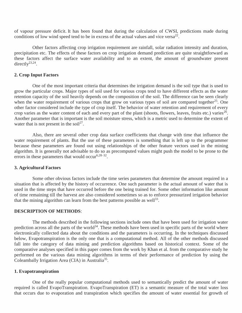
DESCRIPTION OF METHODS:

The methods described in the following sections include ones that have been used for irrigation water

prediction across all the parts of the world34. These methods have been used in specific parts of the world where

electronically collected data about the conditions and the parameters is occurring. In the techniques discussed

below, Evapotranspiration is the only one that is a computational method. All of the other methods discussed

fall into the category of data mining and prediction algorithms based on historical context. Some of the

comparative analyses specified in this paper comes from the work by Khan et al. from the comparative study he

performed on the various data mining algorithms in terms of their performance of prediction by using the

Coleambally Irrigation Area (CIA) in Australia35.

1. Evapotranspiration

One of the really popular computational methods used to semantically predict the amount of water

required is called EvapoTranspiration. EvapoTranspiration (ET) is a semantic measure of the total water loss

that occurs due to evaporation and transpiration which specifies the amount of water essential for growth of

plants. It is expressed as a depth (usually in inches). ET is based on a number of factors that can include: local

temperature, precipitation, cloud cover, solar radiation, and the type of plants you are growing. The rate

expresses the amount of water lost from a cropped surface in units of water depth in a unit area of land taken in

the same units as the depth. The time unit can be an hour, day, decade, month or even an entire growing period

or year. The parameter is usually compared with a Reference EvapoTranspiration (ET0) that is used to study the

demand of water requirement independent of crop type and variations in agricultural practices used. ET0 is used

to compute the ET on a hypothetical grass reference crop with specific characteristics6,36,37.

Since this method involves modeling a scientific equation, there is no learning phase and the

parameters for the day are simply substituted into the equation in order to calculate the score. Since empirical

equations are considered, this method performs poorly on real-time scenarios due to uncertainties that are not

taken into account in these equations.

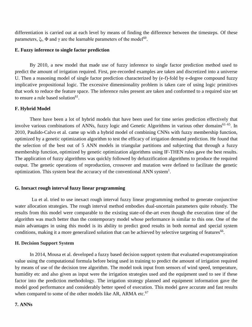
The Evapotranspiration measure is derived from the FAO Penman-Monteith equation is computed as:

where Lv is the volumetric latent heat of vaporization i.e. the energy required per water volume vaporized, E is

the mass water evapotranspiration rate in g / sec m2, ETo is the water volume evapotranspired in mm / sec, Δ is

the rate of change of saturation specific humidity with air temperature in Pa / K, Rn is the net irradiance in W /

m2 which is the external source of energy flux, G is the ground heat flux which is a little difficult to measure, in

W / m2, Cp is the Specific heat capacity of air in J / kg K, ρa is the dry air density in kg / m3, δe is the specific

humidity in Pa ga is the atmospheric conductance in m / s, gs is surface conductance in m / s, γ is the

Psychrometric constant which is close to 66 Pa / K38.

2. Logistic Regression

Logistic regression is a very effective binary classifier that can be used to try to predict the water

requirement as a time series data. Logistic regression can be Simple or Multivariate. Simple logistic regression

is used to predict binary values. In this case, given the amount of water to be used, the model can predict

whether the specification is adequate or not. This is a naive approach and predicted with a rather low accuracy.

Multivariate Logistic Regression takes into account various features to provide decisions39,40. This can

be seen as the simplest feed-forward neural network with one hidden layer and therefore one weight. In this

model, each class specifies the range of water required for irrigation. However, this model does not provide

crop-specific decisions and in no way maps the temporal dependencies35.

Logistic regression is modeled as:

where X is the set of feature vectors of size n, Yi is the predicted class label, W and B are the weights and biases

respectively that would be learned by means of the gradient descent algorithm41.

3. Decision Tree Classifier

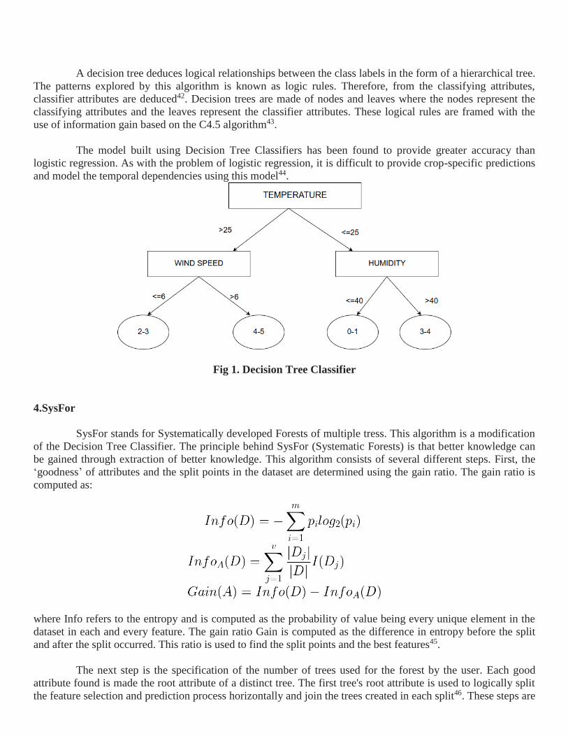
A decision tree deduces logical relationships between the class labels in the form of a hierarchical tree.

The patterns explored by this algorithm is known as logic rules. Therefore, from the classifying attributes,

classifier attributes are deduced42. Decision trees are made of nodes and leaves where the nodes represent the

classifying attributes and the leaves represent the classifier attributes. These logical rules are framed with the

use of information gain based on the C4.5 algorithm43.

The model built using Decision Tree Classifiers has been found to provide greater accuracy than

logistic regression. As with the problem of logistic regression, it is difficult to provide crop-specific predictions

and model the temporal dependencies using this model44.

Fig 1. Decision Tree Classifier

4.SysFor

SysFor stands for Systematically developed Forests of multiple tress. This algorithm is a modification

of the Decision Tree Classifier. The principle behind SysFor (Systematic Forests) is that better knowledge can

be gained through extraction of better knowledge. This algorithm consists of several different steps. First, the

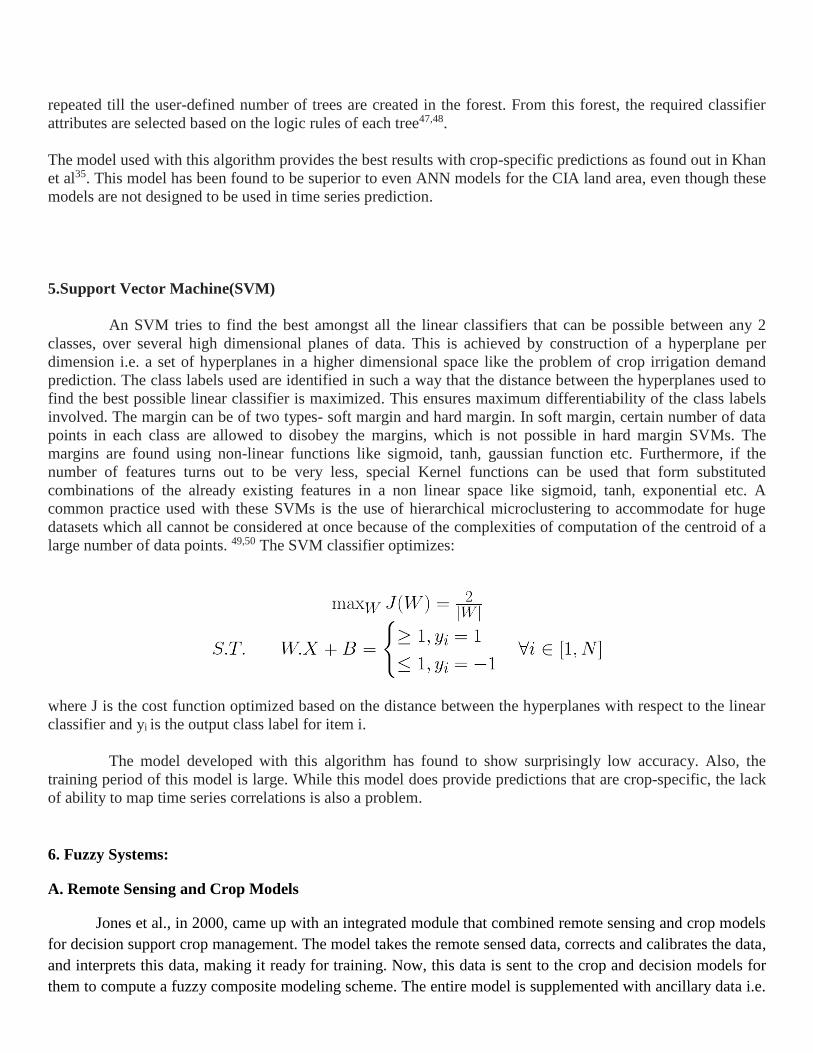
‘goodness’ of attributes and the split points in the dataset are determined using the gain ratio. The gain ratio is

computed as:

where Info refers to the entropy and is computed as the probability of value being every unique element in the

dataset in each and every feature. The gain ratio Gain is computed as the difference in entropy before the split

and after the split occurred. This ratio is used to find the split points and the best features45.

The next step is the specification of the number of trees used for the forest by the user. Each good

attribute found is made the root attribute of a distinct tree. The first tree's root attribute is used to logically split

the feature selection and prediction process horizontally and join the trees created in each split46. These steps are

repeated till the user-defined number of trees are created in the forest. From this forest, the required classifier

attributes are selected based on the logic rules of each tree47,48.

The model used with this algorithm provides the best results with crop-specific predictions as found out in Khan

et al35. This model has been found to be superior to even ANN models for the CIA land area, even though these

models are not designed to be used in time series prediction.

5.Support Vector Machine(SVM)

An SVM tries to find the best amongst all the linear classifiers that can be possible between any 2

classes, over several high dimensional planes of data. This is achieved by construction of a hyperplane per

dimension i.e. a set of hyperplanes in a higher dimensional space like the problem of crop irrigation demand

prediction. The class labels used are identified in such a way that the distance between the hyperplanes used to

find the best possible linear classifier is maximized. This ensures maximum differentiability of the class labels

involved. The margin can be of two types- soft margin and hard margin. In soft margin, certain number of data

points in each class are allowed to disobey the margins, which is not possible in hard margin SVMs. The

margins are found using non-linear functions like sigmoid, tanh, gaussian function etc. Furthermore, if the

number of features turns out to be very less, special Kernel functions can be used that form substituted

combinations of the already existing features in a non linear space like sigmoid, tanh, exponential etc. A

common practice used with these SVMs is the use of hierarchical microclustering to accommodate for huge

datasets which all cannot be considered at once because of the complexities of computation of the centroid of a

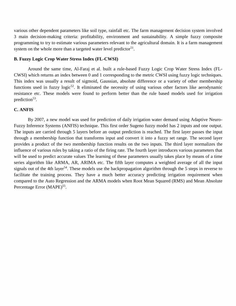
large number of data points. 49,50 The SVM classifier optimizes:

where J is the cost function optimized based on the distance between the hyperplanes with respect to the linear

classifier and yi is the output class label for item i.

The model developed with this algorithm has found to show surprisingly low accuracy. Also, the

training period of this model is large. While this model does provide predictions that are crop-specific, the lack

of ability to map time series correlations is also a problem.

6. Fuzzy Systems:

A. Remote Sensing and Crop Models

Jones et al., in 2000, came up with an integrated module that combined remote sensing and crop models

for decision support crop management. The model takes the remote sensed data, corrects and calibrates the data,

and interprets this data, making it ready for training. Now, this data is sent to the crop and decision models for

them to compute a fuzzy composite modeling scheme. The entire model is supplemented with ancillary data i.e.

various other dependent parameters like soil type, rainfall etc. The farm management decision system involved

3 main decision-making criteria: profitability, environment and sustainability. A simple fuzzy composite

programming to try to estimate various parameters relevant to the agricultural domain. It is a farm management

system on the whole more than a targeted water level predictor51.

B. Fuzzy Logic Crop Water Stress Index (FL-CWSI)

Around the same time, Al-Faraj et al. built a rule-based Fuzzy Logic Crop Water Stress Index (FL-

CWSI) which returns an index between 0 and 1 corresponding to the metric CWSI using fuzzy logic techniques.

This index was usually a result of sigmoid, Gaussian, absolute difference or a variety of other membership

functions used in fuzzy logic52. It eliminated the necessity of using various other factors like aerodynamic

resistance etc. These models were found to perform better than the rule based models used for irrigation

prediction53.

C. ANFIS

By 2007, a new model was used for prediction of daily irrigation water demand using Adaptive Neuro-

Fuzzy Inference Systems (ANFIS) technique. This first order Sugeno fuzzy model has 2 inputs and one output.

The inputs are carried through 5 layers before an output prediction is reached. The first layer passes the input

through a membership function that transforms input and convert it into a fuzzy set range. The second layer

provides a product of the two membership function results on the two inputs. The third layer normalizes the

influence of various rules by taking a ratio of the firing rate. The fourth layer introduces various parameters that

will be used to predict accurate values The learning of these parameters usually takes place by means of a time

series algorithm like ARMA, AR, ARIMA etc. The fifth layer computes a weighted average of all the input

signals out of the 4th layer54. These models use the backpropagation algorithm through the 5 steps in reverse to

facilitate the training process. They have a much better accuracy predicting irrigation requirement when

compared to the Auto Regression and the ARMA models when Root Mean Squared (RMS) and Mean Absolute

Percentage Error (MAPE)55.

Fig 2. ANFIS System with 2 inputs and 1 output

D. ARIMA

In 2009, Wang et al. published a paper surveying the various kernel-based and other AI algorithms that

were used for water flow prediction. Also, the analysis by Landeras et al. in 2009 revealed that the the ARIMA

model and the ANN model, when used for calculation of evapotranspiration, gave a 6-8% reduction in the error

percentage. Also, the work by Wang et al. showed that AR, ARMA, ANFIS models gave much better results

when compared to the ANN models in the domain of water flow prediction56. ARIMA models are generalized

class of models that can predict a stationary time series. Sometimes, stationarity detrending by means of taking

the dth differential and modeling that as a stationary series, non-linear transformations etc. are carried out to

ensure correct predictive results. A stationary series is constant in graph throughout the time series i.e. its

central tendencies tend to remain constant inside of a range. This also acts as a disadvantage to this model as

stationarity is a hard constraint to enforce on the dynamic real time data57–59.

ARIMA(p,d,q) is given by:

where Xt is the predicted output at time step t, µ is the mean over the entire dataset, the summation from

1 to p is the autoregressive model that learns predictions based on a weighted sum of a predefined number of

time step values, the summation from 1 to q is the moving average model that maps the error in prediction of

every time step, ξt is the error parameter that is permitted. The parameter d specifies the number of times the

given input data needs to be differentiated in order to achieve a data distribution that is stationary, where the

differentiation is carried out at each level by means of finding the difference between the timesteps. Of these

parameters, ξt, Φ and γ are the learnable parameters of the model60.

E. Fuzzy inference to single factor prediction

By 2010, a new model that made use of fuzzy inference to single factor prediction method used to

predict the amount of irrigation required. First, pre-recorded examples are taken and discretized into a universe

U. Then a reasoning model of single factor prediction characterized by (e-f)-fold by e-degree compound fuzzy

implicative propositional logic. The excessive dimensionality problem is taken care of using logic primitives

that work to reduce the feature space. The inference rules present are taken and conformed to a required size set

to ensure a rule based solution61.

F. Hybrid Model

There have been a lot of hybrid models that have been used for time series prediction effectively that

involve various combinations of ANNs, fuzzy logic and Genetic Algorithms in various other domains61–65. In

2010, Paulido-Calvo et al. came up with a hybrid model of combining CNNs with fuzzy membership function,

optimized by a genetic optimization algorithm to test the efficacy of irrigation demand prediction. He found that

the selection of the best out of 5 ANN models in triangular partitions and subjecting that through a fuzzy

membership function, optimized by genetic optimization algorithms using IF-THEN rules gave the best results.

The application of fuzzy algorithms was quickly followed by defuzzification algorithms to produce the required

output. The genetic operations of reproduction, crossover and mutation were defined to facilitate the genetic

optimization. This system beat the accuracy of the conventional ANN system1.

G. Inexact rough interval fuzzy linear programming

Lu et al. tried to use inexact rough interval fuzzy linear programming method to generate conjunctive

water allocation strategies. The rough interval method embodies dual-uncertain parameters quite robustly. The

results from this model were comparable to the existing state-of-the-art even though the execution time of the

algorithm was much better than the contemporary model whose performance is similar to this one. One of the

main advantages in using this model is its ability to predict good results in both normal and special system

conditions, making it a more generalized solution that can be achieved by selective targeting of features66.

H. Decision Support System

In 2014, Mousa et al. developed a fuzzy based decision support system that evaluated evapotranspiration

value using the computational formula before being used in training to predict the amount of irrigation required

by means of use of the decision tree algorithm. The model took input from sensors of wind speed, temperature,

humidity etc and also given as input were the irrigation strategies used and the equipment used to see if these

factor into the prediction methodology. The irrigation strategy planned and equipment information gave the

model good performance and considerably better speed of execution. This model gave accurate and fast results

when compared to some of the other models like AR, ARMA etc.67

7. ANNs

Artificial Neural Networks are those architectures in which the input is morphed into a plane where a

linear separation or regression is made possible by means of a non-linearity to warp the input into a plane where

a straight line is enough. Various hyper-parameters used in an ANN would be hidden layer size, number of

hidden layers, batch size, activation function, learning rate, optimization function, initialization strategy and

normalization. The model is trained by means of various training algorithms like BackPropagation, radial basis

function etc. The complexity of what the model can model is usually proportional to the number of layers in the

architecture68–70.

where a is the activation function used, which is usually any number of nonlinearities like sigmoid, tanh etc.

The model is trained as a composition of activation functions that occurs the same number of times as the

number of layers to give the final output. While these models operate in the nonlinear space and have much

more scope for accommodating generic input, these models don’t have the capabilities to map the time series

dependencies found in irrigation demand prediction71.

Around 2001, the performance of artificial neural network architectures was compared with most of the

other models at the time like ARMA, AR, SVMs etc. It was found that ANNs performed consistently worse

than the SMT and the ANFIS models56. But by 2003, ANNs were tweaked efficiently enough to become better

in performance than the other models like ANFIS, ARMA etc.72 Hardaha et al. did extensive work on tweaking

the various parameters of the ANN to give an exploratory understanding on the dependence of each hyper-

parameter to the accuracy of the model. It was found that training based on the radial basis function gave the

best results for prediction of water requirement of wheat crops73.

A. Artificial Neuro-Genetic Networks

A hybrid ANN model that incorporates a genetic algorithm on top of an ANN to improve the accuracy

of the model was proposed in 2009. This model used the Artificial Neuro-Genetic Networks (ANGN) to predict

the irrigation requirement of the crops. Initially, the collection of ANNs of size N are taken to be the entire

population. A first generation would contain an initialized collection of ANNs all with their own hyper-

parameters. The output from the initial population is sent into the ANN chosen is then used to train the

particular input. Now the accuracies of the different models are checked to see which ANGN selection would

result in the best performance. To optimize the entire process, a pareto front is added before the output is

specified. Objective evaluation functions F1 and F2 are first calculated over the entire corpus and are further

used in the ANGN selection process74.

A study by Khan et al. in 2013 compares different AI models and their accuracies when it comes to

irrigation prediction. It was found that of all the models, the model with the 3-fold cross validation multiple

decision trees SysFor model gave the best overall results. But the actual water content required by the crop was

accurately predicted by ANNs really accurately. The difference in error percentage between ANNs and SysFor

was almost 20%. Thus, it was concluded that SysFor, ANN and decision tree techniques are the most suitable

for the task of irrigation prediction35.

COMPARISION OF PERFORMANCES

Model Used Dataset / Study area Time Step Accuracy (%) Reference

Logistic Regression Coleambally, Australia 1 day 56 Khan et al.35

Decision Tree

Classifier

Coleambally, Australia 1 day 74 Khan et al.35

SysFor Coleambally, Australia 1 day 78 Khan et al.35

Support Vector

Machines

Coleambally, Australia 1 day 64 Khan et al.35

Remote Sensing and

Crop Models

MAC, University of Arizona Variable (Rule

Based)

58 to 78 Jones et al.51

FL-CWSI Horticulture Dept., UNL Index – no

time series info

CWSI

Comparison Only

Al-Faraj et al.53

ANFIS Chania in Crete, Greece 1 day MAPE

comparison Only

Atsalakis et al.55

ARIMA Álava, Basque County, Spain 1 week ET Comparison

Only

Landeras et al.59

Fuzzy inference to

Single Factor

Prediction

Shangqiu, Henan, China 1 year Value

Comparison Only

Chen et al.61

Hybrid ANN, Fuzzy,

GA

Cordoba province, Spain 1 day 79.73 (in terms of

20.27 SEP %)

Pulido-Calvo et

al.1

Inexact rough

interval fuzzy

Custom dataset Custom Comparison Only Lu et al.66

Decision Support

System

Baghdad, Iraq (Simulation) 1 month ET Comparison

Only

Mousa et al.67

ANNs Bhakra Canal system,

Rajasthan, India

1 month r2 Comparison

Only

Hardaha et al.73

ANGN Bembézar Irrigation District

(Spain)

1 day 87.37 (in terms of

12.63 SEP %)

Perea et al.74

Table 1 Comparison of Models

Simply using fuzzy system architectures will help capture the randomness in the representation and the

fading of hard boundaries at inflection points, but will not do much about the sequential nature of the data.

ARIMA models take into context the temporal dependencies but only work for univariate regression.

Multivariate regression is essential for irrigation prediction. Even the ANFIS architecture is not designed to

capture time series dependencies. ANNs are very good at prediction based on training, but lack the capability of

inferring semantic meaning from the sequential flow. SVMs and other kernel based methods are designed to be

trained on normal data and will not be able to capture the essential sequential information. ANGN also fails to

map temporal dependencies when reading features and predicting outputs.

PROPOSED MODEL

The above mentioned fallacies have left us in an unfortunate situation of choosing amongst a pool of

ordinary choices and simply settling for whatever accuracy we can obtain. Hence, we propose a novel

methodology of using a sequence learning based recurrent neural network (RNN) model that uses the LSTM

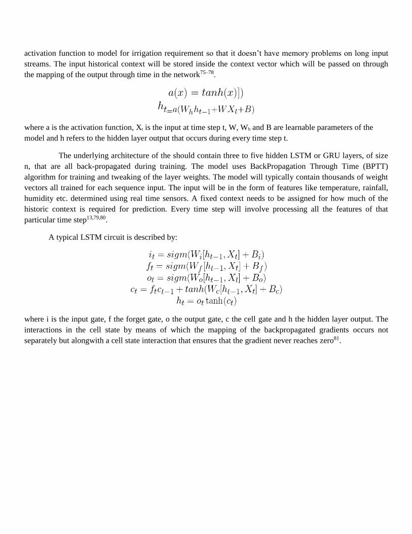
activation function to model for irrigation requirement so that it doesn’t have memory problems on long input

streams. The input historical context will be stored inside the context vector which will be passed on through

the mapping of the output through time in the network75–78.

where a is the activation function, Xt is the input at time step t, W, Wh and B are learnable parameters of the

model and h refers to the hidden layer output that occurs during every time step t.

The underlying architecture of the should contain three to five hidden LSTM or GRU layers, of size

n, that are all back-propagated during training. The model uses BackPropagation Through Time (BPTT)

algorithm for training and tweaking of the layer weights. The model will typically contain thousands of weight

vectors all trained for each sequence input. The input will be in the form of features like temperature, rainfall,

humidity etc. determined using real time sensors. A fixed context needs to be assigned for how much of the

historic context is required for prediction. Every time step will involve processing all the features of that

particular time step13,79,80.

A typical LSTM circuit is described by:

where i is the input gate, f the forget gate, o the output gate, c the cell gate and h the hidden layer output. The

interactions in the cell state by means of which the mapping of the backpropagated gradients occurs not

separately but alongwith a cell state interaction that ensures that the gradient never reaches zero81.

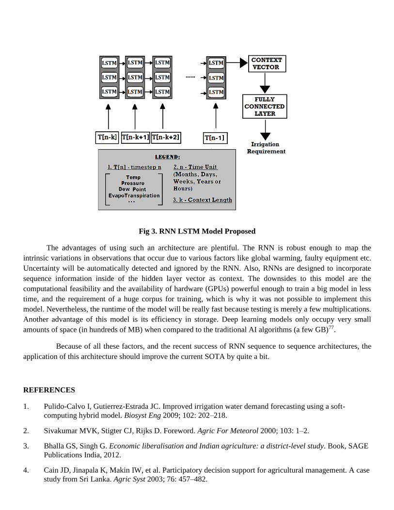
Fig 3. RNN LSTM Model Proposed

The advantages of using such an architecture are plentiful. The RNN is robust enough to map the

intrinsic variations in observations that occur due to various factors like global warming, faulty equipment etc.

Uncertainty will be automatically detected and ignored by the RNN. Also, RNNs are designed to incorporate

sequence information inside of the hidden layer vector as context. The downsides to this model are the

computational feasibility and the availability of hardware (GPUs) powerful enough to train a big model in less

time, and the requirement of a huge corpus for training, which is why it was not possible to implement this

model. Nevertheless, the runtime of the model will be really fast because testing is merely a few multiplications.

Another advantage of this model is its efficiency in storage. Deep learning models only occupy very small

amounts of space (in hundreds of MB) when compared to the traditional AI algorithms (a few GB)77.

Because of all these factors, and the recent success of RNN sequence to sequence architectures, the

application of this architecture should improve the current SOTA by quite a bit.

REFERENCES

1. Pulido-Calvo I, Gutierrez-Estrada JC. Improved irrigation water demand forecasting using a soft-

computing hybrid model. Biosyst Eng 2009; 102: 202–218.

2. Sivakumar MVK, Stigter CJ, Rijks D. Foreword. Agric For Meteorol 2000; 103: 1–2.

3. Bhalla GS, Singh G. Economic liberalisation and Indian agriculture: a district-level study. Book, SAGE

Publications India, 2012.

4. Cain JD, Jinapala K, Makin IW, et al. Participatory decision support for agricultural management. A case

study from Sri Lanka. Agric Syst 2003; 76: 457–482.

5. Singh V, Singh UC. Assessment of groundwater quality of parts of Gwalior (India) for agricultural

purposes. Indian J Sci Technol 2008; 1: 1–5.

6. Allen RG, Pereira LS, Raes D, et al. Crop evapotranspiration-Guidelines for computing crop water

requirements-FAO Irrigation and drainage paper 56. FAO, Rome 1998; 300: D05109.

7. Smith M. CROPWAT: A computer program for irrigation planning and management. Book, Food &

Agriculture Org., 1992.

8. Wu IP. Energy gradient line approach for direct hydraulic calculation in drip irrigation design. Irrig Sci

1992; 13: 21–29.

9. Alvisi S, Franchini M, Marinelli A. A short-term, pattern-based model for water-demand forecasting. J

Hydroinformatics 2007; 9: 39–50.

10. Zhou SL, McMahon TA, Walton A, et al. Forecasting operational demand for an urban water supply

zone. J Hydrol 2002; 259: 189–202.

11. Patel H, Patel D. A Comparative Study on Various Data Mining Algorithms with Special Reference to

Crop Yield Prediction. Indian J Sci Technol; 9.

12. Gers FA, Eck D, Schmidhuber J. Applying LSTM to time series predictable through time-window

approaches. In: International Conference on Artificial Neural Networks. Inproceedings, 2001, pp. 669–

676.

13. Gers FA, Schmidhuber J, Cummins F. Learning to forget: Continual prediction with LSTM. Neural

Comput 2000; 12: 2451–2471.

14. Graves A, Jaitly N, Mohamed A. Hybrid speech recognition with deep bidirectional LSTM. In:

Automatic Speech Recognition and Understanding (ASRU), 2013 IEEE Workshop on. Inproceedings,

2013, pp. 273–278.

15. Graves A, Schmidhuber J. Framewise phoneme classification with bidirectional LSTM and other neural

network architectures. Neural Networks 2005; 18: 602–610.

16. Sundermeyer M, Oparin I, Gauvain J-L, et al. Comparison of feedforward and recurrent neural network

language models. In: 2013 IEEE International Conference on Acoustics, Speech and Signal Processing.

Inproceedings, 2013, pp. 8430–8434.

17. Sak H, Senior A, Beaufays F. Long short-term memory based recurrent neural network architectures for

large vocabulary speech recognition. arXiv Prepr arXiv14021128.

18. Hanks RJ, Hill RW, others. Modeling crop responses to irrigation in relation to soils, climate and

salinity. Book, International Irrigation Information Center., 1980.

19. Murthy ASR, Sudheer Y, Mounika K, et al. Cloud Technology on Agriculture using Sensors. Indian J

Sci Technol; 9.

20. Kumar MK, Ravi KS. Automation of Irrigation System based on Wi-Fi Technology and IOT. Indian J

Sci Technol; 9.

21. Schlenker W, Roberts MJ. Nonlinear temperature effects indicate severe damages to US crop yields

under climate change. Proc Natl Acad Sci 2009; 106: 15594–15598.

22. O’Toole JC, Hatfield JL. Effect of wind on the crop water stress index derived by infrared thermometry.

Agron J 1983; 75: 811–817.

23. Fritschen LJ. Net and solar radiation relations over irrigated field crops. Agric Meteorol 1967; 4: 55–62.

24. Fischer RA. Number of kernels in wheat crops and the influence of solar radiation and temperature. J

Agric Sci 1985; 105: 447–461.

25. Tolk JA, Howell TA, Evett SR. Effect of mulch, irrigation, and soil type on water use and yield of maize.

Soil Tillage Res 1999; 50: 137–147.

26. Rao AVMS, Chandran MAS. Crop water requirements. Agrometeorol Data Collect Anal Manag 1977;

51.

27. Slatyer RO. The influence of progressive increases in total soil moisture stress on transpiration, growth,

and internal water relationships of plants. Aust J Biol Sci 1957; 10: 320–336.

28. Loew A, Ludwig R, Mauser W. Derivation of surface soil moisture from ENVISAT ASAR wide swath

and image mode data in agricultural areas. IEEE Trans Geosci Remote Sens 2006; 44: 889–899.

29. Renard KG, Foster GR, Weesies GA, et al. Predicting soil erosion by water: a guide to conservation

planning with the Revised Universal Soil Loss Equation (RUSLE). Book, US Government Printing Office

Washington, DC, 1997.

30. Moran MS, Clarke TR, Inoue Y, et al. Estimating crop water deficit using the relation between surface-

air temperature and spectral vegetation index. Remote Sens Environ 1994; 49: 246–263.

31. Allen RG. Using the FAO-56 dual crop coefficient method over an irrigated region as part of an

evapotranspiration intercomparison study. J Hydrol 2000; 229: 27–41.

32. Jensen ME, Wright JL, Pratt BJ. Estimating soil moisture depletion from climate, crop and soil data.

Trans ASAE 1971; 14: 954–959.

33. Phocaides A. Technical handbook on pressurized irrigation techniques.

34. Igbadun HE. Irrigation Scheduling Impact Assessment MODel (ISIAMOD): A decision tool for

irrigation scheduling. Indian J Sci Technol 2012; 5: 3090–3099.

35. Khan M.A., Islam M.Z. HM. Evaluating the Performance of Several Data Mining Methods for Predicting

Irrigation Water Requirement. In: Zhao Y. LJKPJ, Christen P (eds) Data Mining and Analytics 2012

(AusDM 2012). Inproceedings, Sydney, Australia: ACS, pp. 199–208.

36. Brouwer C, Heibloem M. Irrigation water management: irrigation water needs. Train Man; 3.

37. Jensen ME, Burman RD, Allen RG. Evapotranspiration and irrigation water requirements. Inproceedings,

1990.

38. Zotarelli L, Dukes MD, Romero CC, et al. Step by step calculation of the Penman-Monteith

Evapotranspiration (FAO-56 Method). Inst Food Agric Sci Univ Florida.

39. Christensen R. Linear models for multivariate, time series, and spatial data. Book, Springer Science &

Business Media, 1991.

40. Christensen R. Log-linear models and logistic regression. Book, Springer Science & Business Media,

2006.

41. Bottou L. Large-scale machine learning with stochastic gradient descent. In: Proceedings of

COMPSTAT’2010. Incollection, Springer, 2010, pp. 177–186.

42. Islam MZ. EXPLORE: A Novel Decision Tree Classification Algorithm. In: MacKinnon LM (ed) Data

Security and Security Data: 27th British National Conference on Databases, BNCOD 27, Dundee, UK,

June 29 - July 1, 2010. Revised Selected Papers. Inbook, Berlin, Heidelberg: Springer Berlin Heidelberg,

pp. 55–71.

43. John GH, Kohavi R, Pfleger K, et al. Irrelevant features and the subset selection problem. In: Machine

learning: proceedings of the eleventh international conference. Inproceedings, 1994, pp. 121–129.

44. Quinlan JR. C4.5: Programs for Machine Learning. Book, San Francisco, CA, USA: Morgan Kaufmann

Publishers Inc., 1993.

45. Quinlan JR. Induction of decision trees. Mach Learn 1986; 1: 81–106.

46. Islam MZ, Giggins H. Knowledge Discovery through SysFor - a Systematically Developed Forest of

Multiple Decision Trees. In: Vamplew P. SAOK-LCP, Kennedy PJ (eds) Australasian Data Mining

Conference (AusDM 11). Inproceedings, Ballarat, Australia: ACS, pp. 195–204.

47. Islam MZ. EXPLORE: a novel decision tree classification algorithm. In: British National Conference on

Databases. Inproceedings, 2010, pp. 55–71.

48. Mitchell TM. Machine learning. 1997. Burr Ridge, McGraw Hill 1997; 45: 37.

49. Burges CJC. A tutorial on support vector machines for pattern recognition. Data Min Knowl Discov

1998; 2: 121–167.

50. Vapnik VN. The Nature of Statistical Learning Theory. Book, New York, NY, USA: Springer-Verlag

New York, Inc., 1995.

51. Jones D, Barnes EM. Fuzzy composite programming to combine remote sensing and crop models for

decision support in precision crop management. Agric Syst 2000; 65: 137–158.

52. Zadeh LA. Fuzzy sets. Inf Control 1965; 8: 338–353.

53. Al-Faraj A, Meyer GE, Horst GL. A crop water stress index for tall fescue (Festuca arundinacea Schreb.)

irrigation decision-making—a traditional method. Comput Electron Agric 2001; 31: 107–124.

54. Jang J-S. ANFIS: adaptive-network-based fuzzy inference system. IEEE Trans Syst Man Cybern 1993;

23: 665–685.

55. Atsalakis G, Minoudaki C, others. Daily irrigation water demand prediction using Adaptive Neuro-Fuzzy

Inferences Systems (ANFIS). Inproceedings.

56. Wang W-C, Chau K-W, Cheng C-T, et al. A comparison of performance of several artificial intelligence

methods for forecasting monthly discharge time series. J Hydrol 2009; 374: 294–306.

57. Box GEP, Pierce DA. Distribution of residual autocorrelations in autoregressive-integrated moving

average time series models. J Am Stat Assoc 1970; 65: 1509–1526.

58. Valipour M, Banihabib ME, Behbahani SMR. Comparison of the ARMA, ARIMA, and the

autoregressive artificial neural network models in forecasting the monthly inflow of Dez dam reservoir. J

Hydrol 2013; 476: 433–441.

59. Landeras G, Ortiz-Barredo A, López JJ. Forecasting weekly evapotranspiration with ARIMA and

artificial neural network models. J Irrig Drain Eng 2009; 135: 323–334.

60. Wei WW-S. Time series analysis. Book, Addison-Wesley publ Reading, 1994.

61. Chen Q, Jing L, Gao Y. Study on Applying Fuzzy Inference to Single Factor Prediction Method for

Precipitation Irrigation Requirement Forecast. In: 2010 2nd International Workshop on Intelligent

Systems and Applications. Inproceedings, 2010.

62. Hassan MR, Nath B, Kirley M. A fusion model of HMM, ANN and GA for stock market forecasting.

Expert Syst Appl 2007; 33: 171–180.

63. Mukerji A, Chatterjee C, Raghuwanshi NS. Flood forecasting using ANN, neuro-fuzzy, and neuro-GA

models. J Hydrol Eng 2009; 14: 647–652.

64. Ruan D, Wang PP. Intelligent hybrid systems: fuzzy logic, neural networks, and genetic algorithms.

Book, Springer, 1997.

65. Kavousi-Fard A. A new fuzzy-based feature selection and hybrid TLA--ANN modelling for short-term

load forecasting. J Exp Theor Artif Intell 2013; 25: 543–557.

66. Lu H, Huang G, He L. An inexact rough-interval fuzzy linear programming method for generating

conjunctive water-allocation strategies to agricultural irrigation systems. Appl Math Model 2011; 35:

4330–4340.

67. Mousa AK, Croock MS, Abdullah MN. Fuzzy based Decision Support Model for Irrigation System

Management. Int J Comput Appl; 104.

68. Yegnanarayana B. Artificial neural networks. Book, PHI Learning Pvt. Ltd., 2009.

69. Raman H, Sunilkumar N. Multivariate modelling of water resources time series using artificial neural

networks. Hydrol Sci J 1995; 40: 145–163.

70. Zhang GP. Time series forecasting using a hybrid ARIMA and neural network model. Neurocomputing

2003; 50: 159–175.

71. Zhang GP, Patuwo BE, Hu MY. A simulation study of artificial neural networks for nonlinear time-series

forecasting. Comput Oper Res 2001; 28: 381–396.

72. Pulido-Calvo I, Roldán J, López-Luque R, et al. Demand forecasting for irrigation water distribution

systems. J Irrig Drain Eng 2003; 129: 422–431.

73. Hardaha MK, Chouhan SS, Ambast SK. APPLICATION OF ARTIFICIAL NEURAL NETWORK IN

PREDICTION OF RESPONSE OF FARMERS’WATER MANAGEMENT DECISIONS ON WHEAT

YIELD. J Indian Water Resour Soc; 32.

74. Perea RG, Poyato EC, Montesinos P, et al. Irrigation Demand Forecasting Using Artificial Neuro-

Genetic Networks. Water Resour Manag 2015; 29: 5551–5567.

75. Medsker LR, Jain LC. Recurrent neural networks. Des Appl.

76. Funahashi K, Nakamura Y. Approximation of dynamical systems by continuous time recurrent neural

networks. Neural networks 1993; 6: 801–806.

77. Connor JT, Martin RD, Atlas LE. Recurrent neural networks and robust time series prediction. IEEE

Trans neural networks 1994; 5: 240–254.

78. Dorffner G. Neural networks for time series processing. In: Neural Network World. Inproceedings, 1996.

79. Werbos PJ. Backpropagation through time: what it does and how to do it. Proc IEEE 1990; 78: 1550–

1560.

80. Mikolov T, Karafiat M, Burget L, et al. Recurrent Neural Network based Language Model. Interspeech

2010; 1045–1048.

81. Hochreiter S, Schmidhuber J. LSTM can solve hard long time lag problems. Adv Neural Inf Process Syst

1997; 473–479.