A Review of Methods for Moving Boundary ProblemsA classic method for describing this moving boundary problem is to shift from the ﬁxed frame of reference associated with the box

Coa

stal

and

Hyd

raul

ics

Labo

rato

ryER

DC

/CH

LTR

-09-

10

Navigation Systems Research Program

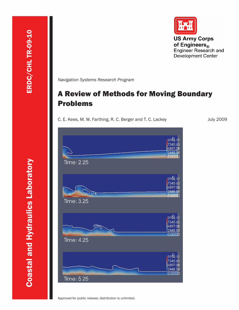
A Review of Methods for Moving BoundaryProblems

C. E. Kees, M. W. Farthing, R. C. Berger and T. C. Lackey July 2009

Approved for public release; distribution is unlimited.

Navigation Systems Research Program ERDC/CHL TR-09-10

July 2009

A Review of Methods for Moving Boundary

Problems

C. E. Kees, M. W. Farthing, R. C. Berger and T. C. Lackey

Coastal and Hydraulics Laboratory

U.S. Army Engineer Research and Development Center

3909 Halls Ferry Road.

Vicksburg, MS 39180-6199

Final Report

Approved for public release; distribution is unlimited.

Prepared for U.S. Army Corps of Engineers

Washington, DC 20314-1000

Under Work Unit KHBCGD

ERDC/CHL TR-09-10 ii

Abstract: State-of-the-art numerical methods for solving moving bound-

ary problems arising from multiphase flow and fluid-structure interaction

modeling are reviewed. The emphasis of the review is on robust methods

that do not require the mesh to conform to the moving boundary. The im-

petus for this review is the Coastal and Hydraulics Laboratory’s mission

in navigation. Accurately predicting the effect of a vessel on a waterway

and the vessel motion are required to support the navigation mission as

is accurately predicting wave interaction with coastal and hydraulic struc-

tures. A key part of making accurate predictions in these cases is solving

moving boundary problems. This report identifies promising directions

for research and development of in-house, state-of-the-art computational

models.

Disclaimer: The contents of this report are not to be used for advertising, publication, or promotional purposes. Citationof trade names does not constitute an official endorsement or approval of the use of such commercial products. All productnames and trademarks cited are the property of their respective owners. The findings of this report are not to be construed asan official Department of the Army position unless so designated by other authorized documents.

DESTROY THIS REPORT WHEN NO LONGER NEEDED. DO NOT RETURN IT TO THE ORIGINATOR.

ERDC/CHL TR-09-10 iii

Table of Contents

List of Figures........................................................................................................ iv

Preface.................................................................................................................. v

1 Introduction .................................................................................................... 1

2 Background .................................................................................................... 3

2.1 Navier-Stokes equations for incompressible, Newtonian fluids............................ 3

2.2 Moving boundary models ............................................................................. 5

3 Current Trends ............................................................................................... 14

3.1 Recent work on free boundary modeling ....................................................... 14

3.2 Recent work on multiphase flow modeling .................................................... 15

3.3 Modeling with unstructured tetrahedral meshes ............................................ 16

4 Conclusions ................................................................................................... 17

References.......................................................................................................... 18

ERDC/CHL TR-09-10 iv

List of Figures

Figure 1. Domain with three mobile phases. .................................................................. 1

Figure 2. Parametric, implicit, and characteristic representations of a surface in R3............. 6

Figure 3. Signed distance level sets for moving boundary at z = 1/2. ................................. 8

Figure 4. Level sets with corners. ............................................................................... 13

ERDC/CHL TR-09-10 v

Preface

This report is a product of the High Fidelity Vessel Effects Work Unit

of the Navigation Systems Research Program being conducted at the

U.S. Army Engineer Research and Development Center, Coastal and Hy-

draulics Laboratory.

The report was prepared by Drs. Christopher E. Kees and Matthew W. Far-

thing under the supervision of Mr. Earl V. Edris, Jr., Chief, Hydrologic

Systems Branch; by Dr. Tahirih C. Lackey under the supervision of Dr. Ty

V. Wamsley, Chief, Coastal Processes Branch; and by Dr. R. C. Berger

under the supervision of Dr. Robert T. McAdory, Chief Estuarine En-

gineering Branch. General supervision was provided by Mr. Thomas

W. Richardson, Director, CHL; Dr. William D. Martin, Deputy Director,

CHL; and Mr. Bruce A. Ebersole, Chief Flood and Storm Protection Divi-

sion.

Technical advice needed to complete this work was provided by Drs. Stacy

E. Howington and Robert S. Bernard, Coastal and Hydraulics Labora-

tory. Typesetting assistance was provided by Ms. Sophia K. Vollor, Coastal

and Hydraulics Laboratory.

Mr. James E. Clausner, Navigation Systems Program Manager, was the

project manager for this effort. Mr. W. Jeff Lillycrop was the Technical

Director.

COL Gary E. Johnston was Commander and Executive Director of the

Engineer Research and Development Center. Dr. James E. Houston was

Director.

This report was typeset by the authors with the LATEX document prepa-

ration system. The report uses the erdc document class and mathgifg

fonts package developed by Dr. Boris Veytsman under the supervision of

Mr. Ryan E. North, Geotechnical and Structures Laboratory. The pack-

ages are available from http://ctan.tug.org.

ERDC/CHL TR-09-10 1

1 Introduction

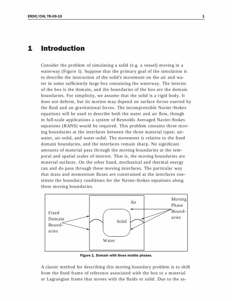
Consider the problem of simulating a solid (e.g. a vessel) moving in a

waterway (Figure 1). Suppose that the primary goal of the simulation is

to describe the interaction of the solid’s movement on the air and wa-

ter in some sufficiently large box containing the waterway. The interior

of the box is the domain, and the boundaries of the box are the domain

boundaries. For simplicity, we assume that the solid is a rigid body. It

does not deform, but its motion may depend on surface forces exerted by

the fluid and on gravitational forces. The incompressible Navier-Stokes

equations will be used to describe both the water and air flow, though

in full-scale applications a system of Reynolds Averaged Navier-Stokes

equations (RANS) would be required. This problem contains three mov-

ing boundaries at the interfaces between the three material types: air-

water, air-solid, and water-solid. The movement is relative to the fixed

domain boundaries, and the interfaces remain sharp. No significant

amounts of material pass through the moving boundaries at the tem-

poral and spatial scales of interest. That is, the moving boundaries are

material surfaces. On the other hand, mechanical and thermal energy

can and do pass through these moving interfaces. The particular way

that mass and momentum fluxes are constrained at the interfaces con-

stitute the boundary conditions for the Navier-Stokes equations along

these moving boundaries.

'

&

$

%Solid

Air

Water

Fixed

Domain

Bound-

aries

:

XXXXXXXXz

Moving

Phase

Bound-

aries

)

Figure 1. Domain with three mobile phases.

A classic method for describing this moving boundary problem is to shift

from the fixed frame of reference associated with the box to a material

or Lagrangian frame that moves with the fluids or solid. Due to the as-

ERDC/CHL TR-09-10 2

sumption that interfaces are material boundaries, the moving bound-

aries in the fixed frame become fixed boundaries in the moving frame

and vice versa. This approach may complicate the application of bound-

ary conditions at the domain boundary, and in the present case it is fur-

ther complicated by the fact that the moving boundaries are moving rel-

ative to one another. The transformation from fixed to moving frame

becomes a part of the solution to the problem–it is based on integra-

tion of the flow velocity. Instead of a purely Lagrangian perspective,

so-called Arbitrary Lagrangian-Eulerian (ALE) space-time formulations

that blend the Lagrangian perspective near the moving boundaries with

the fixed “Eulerian” frame away from moving boundaries are often pre-

ferred (e.g. (Donea, 1982; Hughes and Hulbert, 1998)). The ALE formu-

lation requires additional decisions about the blending of Eulerian and

Lagrangian frames that do not follow from the physics alone. These deci-

sions form part of the solution method.

In many cases, the resulting flow dynamics may cause the material do-

mains to undergo changes in topology. For instance, breaking waves or

flow over the top of the vessel may change the connectedness of the wa-

ter and air domains. The time-dependent space transformation in the

ALE formulations becomes degenerate during such topological changes.

Furthermore, even when no topological changes occur, the numerical

ALE formulation must be carefully designed to prevent numerical insta-

bilities from polluting the results.

This review focuses instead on the fixed or Eulerian perspective because

of the difficulties associated with ALE formulations of the moving bound-

ary problem. We also exclude various other particle-based numerical

methods that can be used to approximate multiphase flow models (e.g.

the Lattice-Boltzmann method (Frisch et al., 1986) and the particle finite

element method (Idelsohn et al., 2006)). For Eulerian approaches, the

primary difficulty becomes accurately locating the moving boundary and

applying boundary conditions there. In the next section we provide some

mathematical background on free boundary problems. Then we review

and discuss the current trends in numerical methods. We conclude with

a list of recommendations for further numerical modeling work.

ERDC/CHL TR-09-10 3

2 Background

We begin by reviewing the basic mathematical framework of moving

boundary problems for two-phase flow. First, we describe the Eulerian

flow model and then popular techniques for modeling the moving bound-

ary.

2.1 Navier-Stokes equations for incompressible, Newtonian fluids

We partition the spatial domain, Ω, into two subdomains Ωw (water) and

Ωa (air). In each subdomain we write the incompressible Navier-Stokes

equations as:

∇ · vα = 0 (1)

∂(ραvα)

∂t+ ∇ · (ραvα ⊗ vα − σα) − ραg = 0 (2)

where α = w, a and σα is the stress tensor, given by

σi,j = −pδi,j + µ

(

∂vi

∂xj

+∂vj

∂xi

)

(3)

We let Γ(t) = ∂Ωw

⋂

∂Ωa. Note that both the subdomains and Γ(t) are

actually time dependent. As a simple example, the boundary conditions

on Γ(t) could be

va − vw = 0 (4)

pa − pw = 0 (5)

The first condition reflects continuity of the normal and tangential com-

ponents of the velocity and the second continuity of the pressure. Or,

equivalently, these jump conditions in the unknowns follow from an as-

sumption of continuity of the mass and momentum flux. While it typi-

cally makes sense to assume that the interface has no mass and therefore

that the mass flux is continuous at points on Γ, the well-known phenom-

ena of surface tension implies that the interface can absorb or impart

momentum. Hence, a more general set of jump conditions is

(va − vw) · n = 0 (6)

(σa − σw) · n = f (7)

ERDC/CHL TR-09-10 4

where f is the the force due to the interface and n is the outward unit

normal vector on Ωw. Surface tension results in a force on the fluid di-

rected entirely in the normal direction and typically given by

f = γw,aκn (8)

where κ is the mean curvature of Γ(t) defined as

κ = −∇ · n (9)

and γw,a is the surface tension coefficient for the air/water interface. For

related formulations see (Harlow and Welch, 1965; Popinet and Zaleski,

1999; Tornberg and Enquist, 2000).

Weak formulation

In order to formulate numerical methods and incorporate the jump con-

ditions, we will use a weak formulation of the Navier-Stokes equation.

For now we consider a domain Ω and assume that Γ cuts through Ω and

divides it into two domains Ωw and Ωa. Multiplying the continuity equa-

tion by a smooth test function w with compact support in Ω, integrating

by parts, and applying the jump condition on the normal component of

the velocity yields

−

∫

Ωw

vw · ∇wdV +

∫

Γ

vww · nwdS −

∫

Ωa

va · ∇wdV +

∫

Γ

vww · nadS = 0 (10)

−

∫

Ω

v · ∇wdV −

∫

Γ

(va − vw)w · ndS = 0 (11)

−

∫

Ω

v · ∇wdV = 0 (12)

where we have defined a global fluid velocity

v =

vw x ∈ Ωw

va x ∈ Ωa

(13)

Treating the momentum equation in the same manner yields

∫

Ω

[

∂(ρv)

∂t− ρg

]

wdV −

∫

Ω

(ρv⊗ v − σ) · ∇w =

∫

Γ

fwdS (14)

ERDC/CHL TR-09-10 5

where

p =

pw x ∈ Ωw

pa x ∈ Ωa

(15)

ρ =

ρw x ∈ Ωw

ρa x ∈ Ωa

(16)

σ =

σw x ∈ Ωw

σa x ∈ Ωa

(17)

Note that in general we only know that v · n is continuous at points on Γ

while v, p, ρ, and µ may be discontinuous. Since the viscosity is always

positive and f acts normal to the interface, however, v may be continu-

ous.

2.2 Moving boundary models

We require a representation for the moving boundary, Γ(t), and an equa-

tion for its evolution. As noted in (Sethian, 2001), there are three classic

mathematical perspectives on representing the boundary. First, Γ(t) can

be given in parametric form,

[

x(ξ, η, t), y(ξ, η, t), z(ξ, η, t)]

= x(ξ, η, t) (18)

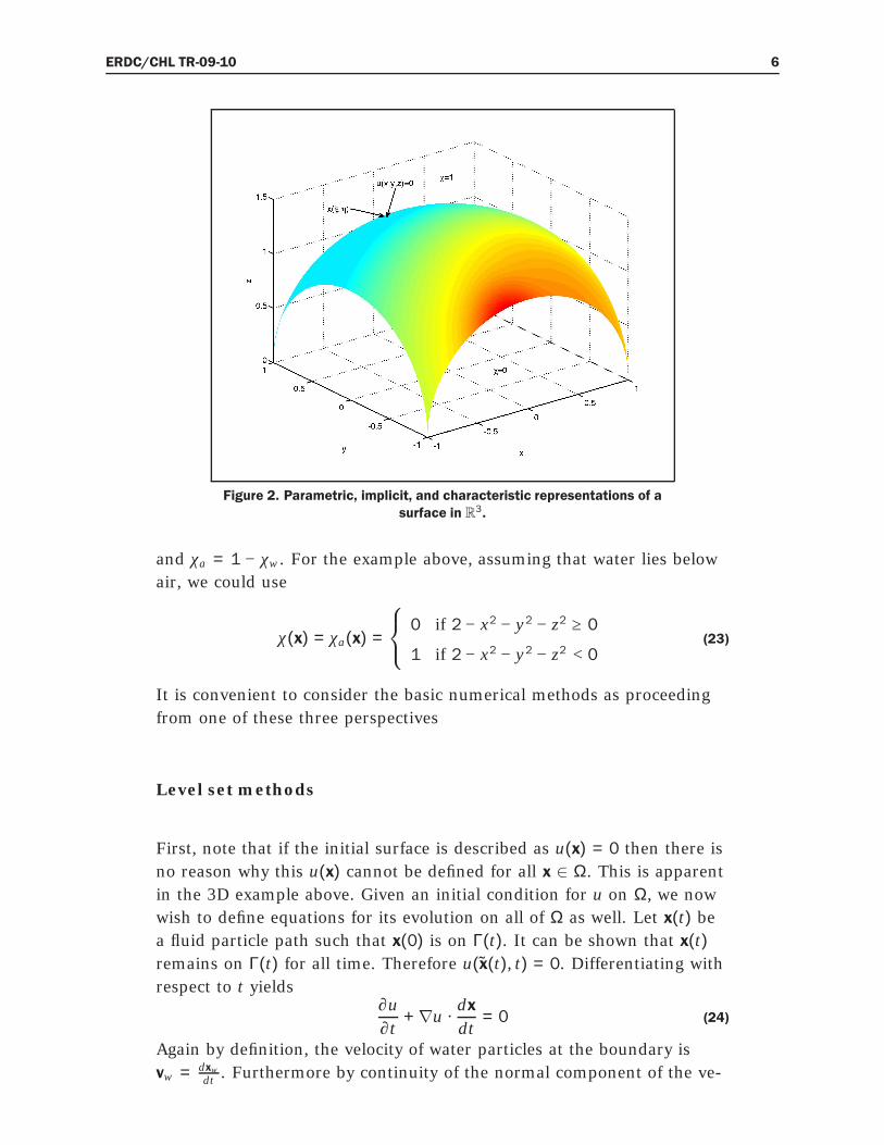
where (ξ, η) ∈ R2 are surface coordinates. For example, the surface de-

picted in figure 2 can be parameterized as

x(x) = (ξ, η,√

2 − ξ2 − η2) (19)

where (ξ, η) ∈ [−1,1]×[−1,1]. Second, Γ(t) can be given in implicit form,

u(x, y, z, t) = u(x, t) = 0 (20)

In the example above we could use

u(x, y, z) = 2 − x2 − y2 − z2 (21)

We will call u a level set (LS) function for the surface since the surface

is given by the zero LS of the function u. Third, instead of representing

Γ(t), the subdomains Ωw and Ωa can be represented in set-theoretic form

via their characteristic functions χw(t) and χa(t) defined by

χw(x) =

1 for x ∈ Ωw

0 for x ∈ Ωa

(22)

ERDC/CHL TR-09-10 6

Figure 2. Parametric, implicit, and characteristic representations of a

surface in R3.

and χa = 1 − χw. For the example above, assuming that water lies below

air, we could use

χ(x) = χa(x) =

0 if 2 − x2 − y2 − z2 ≥ 0

1 if 2 − x2 − y2 − z2 < 0(23)

It is convenient to consider the basic numerical methods as proceeding

from one of these three perspectives

Level set methods

First, note that if the initial surface is described as u(x) = 0 then there is

no reason why this u(x) cannot be defined for all x ∈ Ω. This is apparent

in the 3D example above. Given an initial condition for u on Ω, we now

wish to define equations for its evolution on all of Ω as well. Let x(t) be

a fluid particle path such that x(0) is on Γ(t). It can be shown that x(t)

remains on Γ(t) for all time. Therefore u(x(t), t) = 0. Differentiating with

respect to t yields∂u

∂t+ ∇u ·

dx

dt= 0 (24)

Again by definition, the velocity of water particles at the boundary is

vw = dxwdt

. Furthermore by continuity of the normal component of the ve-

ERDC/CHL TR-09-10 7

locities, we know that on Γ, ∇u · vw = ∇u · va so we can use either velocity

and henceforth drop the subscript. Hence u is related to v through

∂u

∂t+ ∇u · v = 0 (25)

We denote this the non-conservative interface (NCI) equation. Note that

it is known as the kinematic boundary condition for the free surface Γ.

We know from calculus that n = ∇u/‖∇u‖ where ‖ · ‖ is the Euclidean

norm. The normal speed is then

sn = vw ·∇u

‖∇u‖=

−∂u∂t

‖∇u‖(26)

We can thus rewrite the NCI equation in terms of the normal speed as a

Hamilton-Jacobi interface (HJI) equation

∂u

∂t+ ‖∇u‖sn = 0 (27)

For the special case of ∇ · v = 0 we can also rewrite the NCI equation as

a conservative interface (CI) equation

∂u

∂t+ ∇ · (uv) = 0 (28)

Note that v need only agree with the physical velocity along Γ, and in

fact many implicit representions of Γ are possible that agree only on Γ.

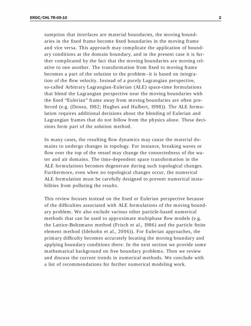
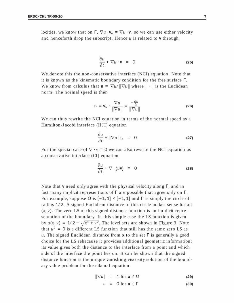
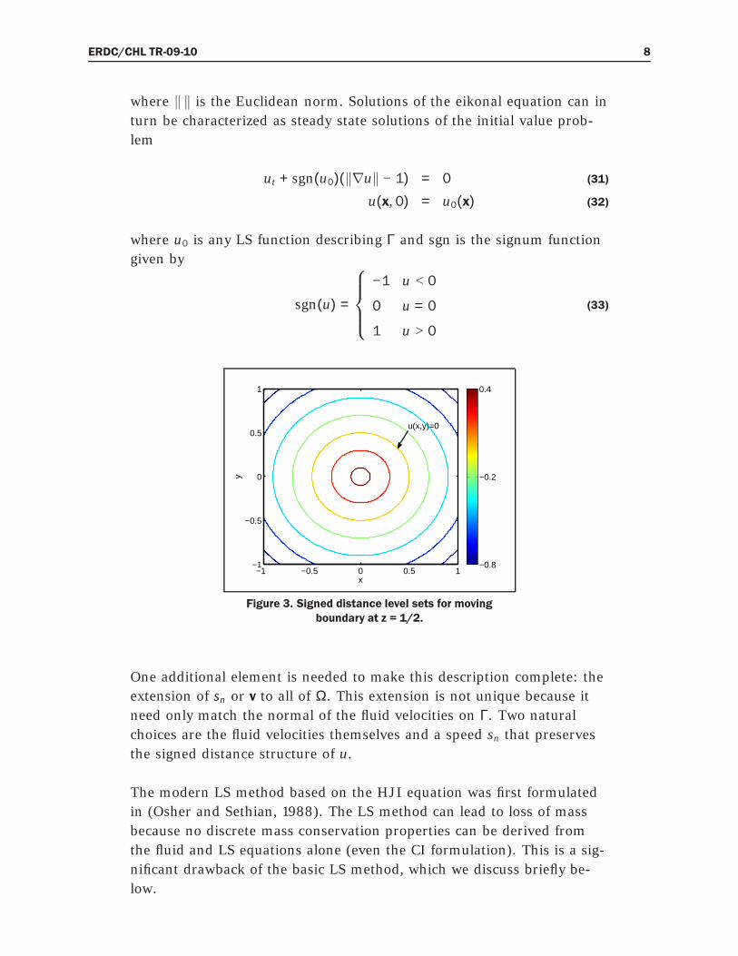
For example, suppose Ω is [−1,1] × [−1,1] and Γ is simply the circle of

radius 1/2. A signed Euclidean distance to this circle makes sense for all

(x, y). The zero LS of this signed distance function is an implicit repre-

sentation of the boundary. In this simple case the LS function is given

by u(x, y) = 1/2 −√

x2 + y2. The level sets are shown in Figure 3. Note

that u2 = 0 is a different LS function that still has the same zero LS as

u. The signed Euclidean distance from x to the set Γ is generally a good

choice for the LS rebecause it provides additional geometric information:

its value gives both the distance to the interface from a point and which

side of the interface the point lies on. It can be shown that the signed

distance function is the unique vanishing viscosity solution of the bound-

ary value problem for the eikonal equation:

‖∇u‖ = 1 for x ∈ Ω (29)

u = 0 for x ∈ Γ (30)

ERDC/CHL TR-09-10 8

where ‖ ‖ is the Euclidean norm. Solutions of the eikonal equation can in

turn be characterized as steady state solutions of the initial value prob-

lem

ut + sgn(u0)(‖∇u‖ − 1) = 0 (31)

u(x,0) = u0(x) (32)

where u0 is any LS function describing Γ and sgn is the signum function

given by

sgn(u) =

−1 u < 0

0 u = 0

1 u > 0

(33)

x

y

−1 −0.5 0 0.5 1−1

−0.5

0

0.5

1

−0.8

−0.2

0.4

u(x,y)=0

Figure 3. Signed distance level sets for moving

boundary at z = 1/2.

One additional element is needed to make this description complete: the

extension of sn or v to all of Ω. This extension is not unique because it

need only match the normal of the fluid velocities on Γ. Two natural

choices are the fluid velocities themselves and a speed sn that preserves

the signed distance structure of u.

The modern LS method based on the HJI equation was first formulated

in (Osher and Sethian, 1988). The LS method can lead to loss of mass

because no discrete mass conservation properties can be derived from

the fluid and LS equations alone (even the CI formulation). This is a sig-

nificant drawback of the basic LS method, which we discuss briefly be-

low.

ERDC/CHL TR-09-10 9

To complete the method for modeling two-phase flow we combine the LS

representation with the two-phase Navier-Stokes formulation. As an ex-

ample we choose to preserve a signed distance representation of the LS

using the eikonal equation and use the NCI equation for the LS dynam-

ics. The complete system of equations in weak form is

∫

Ω

(‖∇u‖ − 1) wdV = 0 (34)

−

∫

Ω

v · ∇wdV =

∫

ΓN,ρ

qρdS (35)

∫

Ω

[

∂(ρv)

∂t−ρg

]

wdV −

∫

Ω

(ρv⊗ v −σ) · ∇w =

∫

Γ

fdS +

∫

ΓN,v

qvdS (36)

∫

Ω

(

∂u

∂t+ ∇u · v

)

w = 0 (37)

where

ρ = ρaH(u) + ρw

[

1 − H(u)]

(38)

µ = µaH(u) + µw

[

1 − H(u)]

(39)

H(u) =

0 u < 0

12

u = 0

1 u > 0

(40)

and the boundary and initial conditions are

u = u for x ∈ Γ (41)

p = pd for x ∈ ΓD,p (42)

v = vd for x ∈ ΓD,v (43)

v · n = qρ(x, t) for x ∈ ΓN,ρ (44)

(ρv⊗ v − σ) · n = qv for x ∈ ΓN,v (45)

p = p0 for x ∈ Ω, t = 0 (46)

v = v0 for x ∈ Ω, t = 0 (47)

u = u0 for x ∈ Ω, t = 0 (48)

Note that equation 34 “redistances” or “re-initializes” u so that the flow

equations are always able to depend on a LS description that provides

the signed distance to the interface. This system is typically solved using

operator splitting. For example, the solution at time ∆t can be approx-

imated by first solving equation 34 (redistance), then solving equations

35 and 36 (Navier-Stokes) using u(0), then finally equation 37 (LS) at

ERDC/CHL TR-09-10 10

t = ∆t using v(∆t). A common variant of this approach is to use smooth

(regularized) approximations of the Heaviside function, H, and the Dirac

delta function to evaluate the discontinuous coefficients and surface force

integral:

ρ ≈ ρaHǫ(u) + ρw

[

1 − Hǫ(u)

]

(49)

µ ≈ µaHǫ(u) + µw

[

1 − Hǫ(u)

]

(50)∫

Γ

fdS ≈

∫

Ω

δǫ(u)f‖∇u‖dV (51)

Hǫ(u) =

0 u < −ǫ

12

(

1 + uǫ

+sin( πu

ǫ)

π

)

u = 0

1 u > ǫ

(52)

δǫ(u) =

0 u < −ǫ

12

(

1ǫ

+cos( πu

ǫ)

ǫ

)

u = 0

0 u > ǫ

(53)

where ǫ is a mesh-dependent parameter (e.g. ǫ = 1.5∆x is recommended

in (Osher and Fedkiw, 2003)). It was pointed out in (Tornberg and En-

quist, 2003) that these simple regularizations of the Heaviside and Dirac

functions are inaccurate and that significantly better alternatives exist.

Furthermore, direct evaluation of the surface force term is also feasi-

ble as are related immersed boundary methods described in (Li and Ito,

2006). It is also common in surface tension calculations to introduce a

filtering step to remove high frequency oscillations from the surface nor-

mal ‖∇u‖ or κ (Tornberg and Enquist, 2000).

We note that the primary advantage of the LS formulation is that accu-

rate and efficient finite element and finite volume methods exist for solv-

ing equations 34–37. Such methods automatically compute the viscosity

solutions for the LS functions, which are the correct solutions for cases

in which the connectivity of the fluid regions change (i.e. during break-

ing or merging of the fluid regions).

Before continuing we consider the conservation properties of the basic

LS method. The mass of water in the domain is given by

∫

Ωw

ρwdV =

∫

Ω

ρwH(u)dV (54)


The integral form of mass conservation can likewise be extended to the

entire domain or any subdomain as

∂

∂t

∫

Ω

ρwH(u)dV +

∫

∂Ω

ρwH(u)vw · nwdS (55)

Of course, for incompressible fluids this implies volume conservation as

well so that we could cancel out ρw. Neither a global nor a local state-

ment of mass or volume conservation can be obtained from any of the

LS equations derived above.

Front tracking (parametric) methods

Next we consider the parametric representation of the surface, x(ξ, η, t).

It is easy to show from the implicit representation of Γ(t) that dxdt

· n = sn,

hence the front tracking (FT) formulation can be written as

dx

dt= vFT (56)

where vFT is any velocity such that vFT · n = sn. Given a discrete repre-

sentation of the x(ξ, η, t) the FT equation is set of (uncoupled) ordinary

differential equations. Early examples of FT for two-phase flow include

(Glimm et al., 1987; Tryggvason and Unverdi, 1990; Unverdi and Tryg-

gvason, 1992). The primary drawback of FT is that for many realistic ve-

locities, the trajectories defined by vFT intersect, leading to degeneracy in

the parametric representation. These problems can be dealt with using

additional, rather complex, “untangling” algorithms based on additional

physical and geometric information (Glimm et al., 1988). We consider

these methods Eulerian methods because the underlying mesh for resolv-

ing physics is fixed, even though the Lagrangian particle tracking is a key

part of the method. Given an implementation of a complete algorithm,

the two-phase model is similar in overall design to the LS model above,

with the exception that the LS advection step is replaced by the FT step

and the coefficients are evaluated using the parametric form of the sur-

face.

Volume of fluid methods

This approach could be described as “pseudo-mixture theory” because

the set characteristic functions χw and χa are derived from the volume


fraction of each discrete cell or element, as if it were filled with a mix-

ture of the two fluids. Instead of solving the free boundary problem ex-

plicitly, the entire fluid domain is described by a single set of equations

for the two-fluid mixture with a particular choice of “constitutive laws”

for the mixture properties. Let θe(x, t) be the ratio of water volume to

total fluid volume in a computational element e. If initially all elements

contain either water or air then θe = χw. We then define the density and

viscosity of the two-fluid mixture as

ρ = θρw + (1 − θ)ρa (57)

µ = θµw + (1 − θ)µa (58)

In a sense these are “constitutive laws” of the mixture, though they are

introduced as a numerical convenience as are the smoothed Heaviside

functions in the LS methods. The flow equations for the mixture are sim-

ply the Navier-Stokes equations for the fluid mixture, which necessarily

has variable density and viscosity (though it is still incompressible). An

additional transport equation for θw represents conservation of volume

for either phase:

θt + ∇ · (θv) = 0 (59)

where v is the velocity of the fluid mixture. Since mass conservation is

explicitly enforced one need only discretize carefully in order to conserve

mass in the fully discrete model. On the other hand, Eulerian methods

for the volume of fluid (VOF) equation tend to smear the jumps in θ,

which results in a loss of information about the precise location of Γ. In-

terface reconstruction and sharpening techniques must be used to coun-

teract this problem and to obtain precise information on the interface

geometry. Early work on VOF methods includes (Noh and Woodward,

1976; Hirt and Nichols, 1981)

Relationships among interface representations

We now relate the FT and VOF interface representations to the LS rep-

resentation. The simplest relationship is among solutions. Given a para-

metric representation xmp(ξ, η, t) then the signed distance LS function is

given by u(x, t) = min(ξ,η) ‖x − xmp(ξ, η, t)‖. Given a signed distance LS

function u(x, t) (u < 0 being the water phase) the characteristic function

is θ = 1−H(u(x, t)) where H is the Heaviside function defined in equation

40


The methods for obtaining solutions are also related. We can rewrite the

HJI equation as

ut + ∇u · (snn) = 0 (60)

This equation is the directional derivative along the curve determined by

the characteristic equations

dxs

dt= snn (61)

xs(0) = x(s,0) (62)

which are equations for a FT representation. Thus, if the FT equations

can be solved then the HJI equation can be as well via

u(xs(t), t) = u(xs(0),0) and whatever method is used to extend u to all of

space. It is well known that the method of characteristics does not yield

the solution of the HJI equations for large time because the character-

istics trajectories, xs(t), will cross in many settings as mentioned above.

On the other hand, the theory of viscosity solutions yields a method for

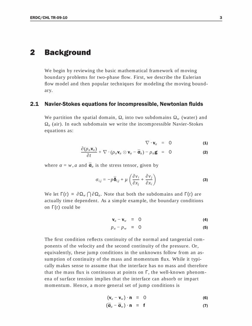
extending solutions of the HJI equation past the point when character-

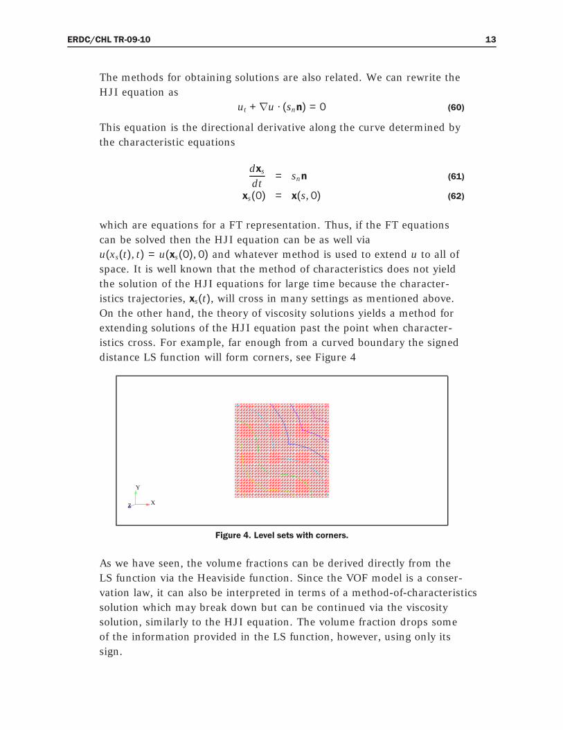
istics cross. For example, far enough from a curved boundary the signed

distance LS function will form corners, see Figure 4

Y

XZ

Figure 4. Level sets with corners.

As we have seen, the volume fractions can be derived directly from the

LS function via the Heaviside function. Since the VOF model is a conser-

vation law, it can also be interpreted in terms of a method-of-characteristics

solution which may break down but can be continued via the viscosity

solution, similarly to the HJI equation. The volume fraction drops some

of the information provided in the LS function, however, using only its

sign.


3 Current Trends

Each basic method or viewpoint has strengths and weaknesses:

• FT methods give very accurate representations of smooth interfaces.

They require complex untangling algorithms to deal with topological

changes and are not strictly mass or volume conserving.

• LS methods that deal with topological changes are easy to implement.

They are not strictly mass or volume conserving and tend to be less

accurate than FT methods.

• VOF methods are strictly mass conserving. They can deal with topo-

logical changes, but they tend to be the least accurate of the three

methods.

The following advice from (Sethian, 2001)

Good numerics is ultimately about getting things to work; the

slavish and blind devotion to one approach above all others is

usually a sign of unfamiliarity with the range of troubles and chal-

lenges presented by real applications.

Much of the recent work on Eulerian methods reflects attempts at com-

bining aspects of all three methods in order to obtain the best properties

of all the methods.

3.1 Recent work on free boundary modeling

One approach to improve the mass conservation properties of LS meth-

ods is the conservative LS/VOF (CLSVOF) method (Sussman and Puck-

ett, 2000). In this approach both the VOF and LS representations are

computed and the VOF function is used to obtain the correct mass. The

CLSVOF method is currently being modified and extended to problems

with surface tension (Sussman, 2003; Sussman et al., 2007). A related

approach simply uses a LS function that mimics a smoothed Heaviside


function rather than a signed distance function in order to mimic the

shape of the set characteristic function (Olsson and Kreiss, 2005).

A different approach to maintaining mass conservation and improving

the resolution of LS methods is the particle-LS method presented in (En-

right et al., 2002). This approach seeds both sides of the interface with

“fluid” particles that are then used to correct the interface. This method

improves the mass conservation properties of the method. Lagrangian

tracking ideas are also being explored to improve the accuracy of low or-

der methods for the LS advection (Enright et al., 2005).

Much of the research on VOF methods has focused on obtaining higher

accuracy and better representations of the interface geometry. The orig-

inal piecewise linear interface reconstruction technique (PLIC) (Youngs,

1982) has been improved upon using parabolic (PROST) (Renardy and

Renardy, 2002) and least squares (Puckett et al., 1997) techniques. A

nice set of comparisons presented in (Gerlach et al., 2006) indicated that

the CLSVOF was generally superior than most state-of-the-art recon-

struction techniques based purely on VOF. Other notable comparisons

of reconstruction algorithms include (Rider and Kothe, 1995; Pilliod and

Pucket, 1997; Rider and Kothe, 1998; Scardovelli and Zaleski, 2003)

The FT research has also continued to mature so that three-dimensional

simulations of problems with complex topological changes are now pos-

sible. A recent set of comparisons and a freely available library of FT

tools are described in (Du et al., 2006).

Other recent directions in LS research includes the use of various meth-

ods for enriching the finite element space locally (Coppola-Owen and Co-

dina, 2005; Chessa and Belytschko, 2003). The particle finite element

methods of (Idelsohn et al., 2006) is a promising new Lagrangian tech-

nique that may challenge Eulerian methods even with respect to robust-

ness.

3.2 Recent work on multiphase flow modeling

Recently, (Kadioglu et al., 2005) used LS methods for modeling under-

water explosions requiring both compressible and incompressible flow

over a wide range of Mach number. Of particular interest to inland nav-

igation is (Price and Chen, 2006), which considers a standard LS for-

mulation of two-phase flow for free surface waves. Reynolds-averaged

Navier-Stokes equations are used to model the fluid flow while a smoothed


Heaviside function is used for material properties (surface tension is ne-

glected). The signed distance property is preserved by time marching the

eikonal equation to equilibrium. Problems considered include oscillating

flow in a tank (sloshing), a dam break problem, and a ship hull moving

in calm water. Another interesting application is the physics-based sim-

ulations described in (Irving et al., 2006), which combines some aspects

of shallow-water modeling with three-phase Navier-Stokes/solid body

modeling.

3.3 Modeling with unstructured tetrahedral meshes

Most of the the methods above are compatible with unstructured meshes,

but much of the work has been carried out on Cartesian meshes. The LS

method was extended to triangular and tetrahedral meshes in (Barth and

Sethian, 1998). That method was extended to air/water flow in porous

media in (Holm and Langtangen, 1999). Recently (Nagrath et al., 2005)

use stabilized finite element for two-phase flow using LSs with a smoothed

Heaviside function for material properties. A discontinuous Galerkin

method appropriate for unstructured meshes is given in (Marchandise

et al., 2006). VOF methods have also been extended to triangular and

tetrahedral meshes (Aliabadi et al., 2003; Tezduyar et al., 1998).


4 Conclusions

We have reviewed a range of methods for accurately and efficiently solv-

ing two- and three-phase boundary problems. There is as yet no consen-

sus on a best method. Instead, there is still much activity in the area of

computational physics and engineering directed at deriving improved al-

gorithms by combining mass/volume conservation, particle tracking, and

LS methods. Given that state of affairs we conclude that

1. A mass conservative hybrid method organized around a core LS im-

plementation is the most practical choice for initial development, hav-

ing a good mix of robustness, accuracy, and efficiency. Additionally,

the tools will have a wide range of applicability outside of two- and

three-phase flow.

2. Including Lagrangian (particle path) information has consistently

been a route toward higher accuracy results so that some form of par-

ticle tracking will likely also be involved in an effective algorithm. We

should begin experimenting with both hybrid particle-LS methods

and the more complex open source FT implementations.

3. Completion of a two-phase test set (e.g. (Rider and Kothe, 1995; Du

et al., 2006)) should be the highest priority for the next phase of the

project. A test set will allow quantitative studies of accuracy and ef-

ficiency on problems of concern to inland navigation as well as guide

laboratory and field data collection for model validation.


References

Aliabadi, S., J. Abedi, and B. Zellars (2003). Parallel finite element simulation of moor-ing forces on floating objects. International Journal for Numerical Methods inFluids 41, 809–822.

Barth, T. J. and J. A. Sethian (1998). Numerical schemes for the hamilton-jacobi and levelset equations on triangulated domains. Journal of Computational Physics 145,1–40.

Chessa, J. and T. Belytschko (2003). A extended finite element method for two-phasefluids. Journal of Applied Mechanics 70, 10–17.

Coppola-Owen, A. H. and R. Codina (2005). Improving eulerian two-phase flow finiteelement approximation with discontinuous gradient pressure shape functions.International Journal for Numerical Methods in Fluids 49, 1287–1304.

Donea, J. (1982). An arbitrary lagrangian-eulerian finite element method for transientfluid-structure interactions. Computational Mechanics 33, 689–723.

Du, J., B. Fix, J. Glimm, X. Jia, Y. Li, and L. Wu (2006). A simple package for front track-ing. Journal of Computational Physics 213, 613–628.

Enright, D., R. Fedkiw, J. Ferziger, and I. Mitchell (2002). A hybrid particle level setmethod for improved interface capturing. Journal of Computational Physics 183,83–116.

Enright, D., F. Losasso, and R. Fedkiw (2005). A fast and accurate semi-lagrangian parti-cle level set method. Computers and Structures 83, 479–490.

Frisch, U., B. Hasslacher, and Y. Pomeau (1986). Lattice gas automata for the Navier–Stokes equation. Physical Review Letters 56(14), 1505–1508.

Gerlach, D., G. Tomar, G. Biswas, and F. Durst (2006). Comparison of volumne-of-fluidmethods for surface tension-dominant two-phase flows. International Journal ofHeat and Mass Transfer 49, 740–754.

Glimm, J., J. Grove, B. Lindquist, O. A. McBryant, and G. Trygvason (1988). The bifurca-tion of tracked scalar waves. SIAM Journal on Scientific and Statistical Comput-ing 9, 61–79.

Glimm, J., O. McBryan, R. Menikoff, and D. H. Sharp (1987). Front tracking applied torayleigh-taylor instability. SIAM Journal on Scientific and Statistical Comput-ing 7, 230–251.

Harlow, F. H. and J. E. Welch (1965). Numerical calculation of time-dependent viscousincompressible flow of fluid with free surface. Physics of Fluids 8(12), 2182–2189.

Hirt, C. W. and B. D. Nichols (1981). Volume of fluid (vof) method for the dynamics offree boundaries. Journal of Computational Physics 39, 201–225.


Holm, E. J. and H. P. Langtangen (1999). A method for simulating sharp fluid interfacesin groundwater flow. Advances in Water Resources 23, 83–95.

Hughes, T. J. R. and G. M. Hulbert (1998). Space-time finite element methods for elas-todynamics: formulations and error estimates. Computer Methods in AppliedMechanics and Engineering 66, 339–363.

Idelsohn, S. R., E. Onate, F. D. Pin, and N. Calvo (2006). Fluid-structure interaction usingthe particle finite element method. Computer Methods in Applied Mechanics andEngineering 195(17-18), 2100–2123.

Irving, G., E. Guendelman, F. Lossaso, and R. Fedkiw (2006). Efficient simulation oflarge bodies of water by coupling two and three dimensional techniques. ACMTransactions on Graphics 25, 805–811.

Kadioglu, S. Y., M. Sussman, S. Osher, J. P. Wright, and M. Kang (2005). A second or-der primitive preconditioner for solving all speed multi-phase flows. Journal ofComputational Physics 209, 477–503.

Li, Z. and K. Ito (2006). The Immersed Interface Method: Numerical Solutions of PDEsInvolving Interfaces and Irregular Domains. Frontiers in Applied Mathematics.Philadelphia: SIAM.

Marchandise, E., J.-F. Remacle, and N. Chevaugeon (2006). A quadrature-free discon-tinuous galerkin method for the level set equation. Journal of ComputationalPhysics 212, 338–357.

Nagrath, S., K. E. Jansen, and R. T. J. Lahey (2005). Computation of incompressiblebubble dynamics with a stabilized finite element level set method. ComputerMethods in Applied Mechanics and Engineering 194, 4565–4587.

Noh, W. F. and P. R. Woodward (1976). Slic (simple line interface calculations). InA. I. van der Vooren and P. J. Zandbergen (Eds.), Lecture Notes in Physics, Vol-ume 59, pp. 330–340. Springer-Verlag.

Olsson, E. and G. Kreiss (2005). A conservative level set method for two phase flow. Jour-nal of Computational Physics 210(1), 225–246.

Osher, S. and R. Fedkiw (2003). Level Set Methods and Dynamic Implicit Surfaces,Volume 153 of Applied Mathematical Sciences. New York: Springer-Verlag.

Osher, S. and J. A. Sethian (1988). Fronts propagating with curvature-dependent speed:algorithms based on hamilton-jacobi formulations. Journal of ComputationalPhysics 79, 12–49.

Pilliod, J. E. J. and E. G. Pucket (1997). Second-order accurate volume-of-fluid algorithmsfor tracking material interfaces. Technical Report LBNL-40744, Lawrence Berke-ley National Laboratory.

Popinet, S. and S. Zaleski (1999). A front-tracking algorithm for accurate representationof surface tension. International Journal for Numerical Methods in Fluids 30,775–793.

Price, W. G. and Y. G. Chen (2006). A simulation of free surface waves for incompressibletwo-phase flows using a curvilinear level set formulation. International Journalfor Numerical Methods in Fluids 51(3), 305–330.


Puckett, E. G., A. S. Almgren, J. B. Bell, D. L. Marcus, and W. J. Rider (1997). A high-order projection method for tracking fluid interfaces in variable density incom-pressible flows. Journal of Computational Physics 130, 269–282.

Renardy, Y. and M. Renardy (2002). Prost: a parabolic reconstruction of surface tension.Journal of Computational Physics 183, 400–421.

Rider, W. J. and D. B. Kothe (1995). Stretching and tearing interface tracking methods.12th AIAA Computational Fluid Dynamics Conference: June 19-22, 1995, SanDiego, CA 2, 806–816.

Rider, W. J. and D. B. Kothe (1998). Reconstructing volume tracking. Journal of Compu-tational Physics 141, 112–152.

Scardovelli, R. and S. Zaleski (2003). Interface reconstruction with least-square fit andsplit eulerian-lagrangian advection. International Journal for Numerical Meth-ods in Fluids 41, 251–274.

Sethian, J. A. (2001). Evolution, implementation, and application of level set and fastmarching methods for advancing fronts. Journal of Computational Physics 169,503–555.

Sussman, M. (2003). A second order coupled level set and volume-of-fluid method forcomputing growth and collapse of vapor bubbles. Journal of ComputationalPhysics 187, 110–136.

Sussman, M. and E. G. Puckett (2000). A coupled level set and volume of fluid methodfor computing 3d and axisymmetric incompressible two-phase flows. Journal ofComputational Phyics 162, 301–337.

Sussman, M., K. M. Smith, M. Y. Hussaini, M. Ohta, and R. Zhi-Wei (2007). A sharpinterface method for incompressible two-phase flows. Journal of ComputationalPhysics 221(2), 469–505.

Tezduyar, T., S. Aliabadi, and M. Behr (1998). Enhanced-discretization interface-capturing technique (edict) for computation of unsteady flows with interfaces.Computer Methods in Applied Mechanics and Engineering 155, 235–248.

Tornberg, A. and B. Enquist (2000). A finite element based level-set method for multi-phase flow applications. Computing and Visualization Science 3, 93–101.

Tornberg, A. and B. Enquist (2003). Regularization techniques for numerical approxima-tion of pdes with singularities. Journal of Scientific Computing 19(1-3), 527–552.

Tryggvason, G. and S. O. Unverdi (1990). Computations of three-dimensional rayleigh-taylor instability. Physics of Fluids 2, 656–659.

Unverdi, S. O. and G. Tryggvason (1992). A front-tracking method for viscous, incom-pressible, multi-fluid flows. Journal of Computational Physics 100, 25–37.

Youngs, D. L. (1982). Time-dependent multi-material flow with large fluid distortion. InK. Morton and M. Baines (Eds.), Numerical Methods for Fluids Dynamics, pp.273–285. New York: Academic Press.

REPORT DOCUMENTATION PAGE Form Approved

OMB No. 0704-0188 Public reporting burden for this collection of information is estimated to average 1 hour per response, including the time for reviewing instructions, searching existing data sources, gathering and maintaining the data needed, and completing and reviewing this collection of information. Send comments regarding this burden estimate or any other aspect of this collection of information, including suggestions for reducing this burden to Department of Defense, Washington Headquarters Services, Directorate for Information Operations and Reports (0704-0188), 1215 Jefferson Davis Highway, Suite 1204, Arlington, VA 22202-4302. Respondents should be aware that notwithstanding any other provision of law, no person shall be subject to any penalty for failing to comply with a collection of information if it does not display a currently valid OMB control number. PLEASE DO NOT RETURN YOUR FORM TO THE ABOVE ADDRESS.

1. REPORT DATE (DD-MM-YYYY) July 2009

2. REPORT TYPE Final

3. DATES COVERED (From - To)

5a. CONTRACT NUMBER

5b. GRANT NUMBER

4. TITLE AND SUBTITLE

A Review of Methods for Moving Boundary Problems

5c. PROGRAM ELEMENT NUMBER

5d. PROJECT NUMBER

5e. TASK NUMBER

6. AUTHOR(S)

C.E. Kees, M.W. Farthing, R.C. Berger and T.C. Lackey

5f. WORK UNIT NUMBER KHBCGD

7. PERFORMING ORGANIZATION NAME(S) AND ADDRESS(ES) 8. PERFORMING ORGANIZATION REPORT NUMBER

U.S. Army Engineer Research and Development Center Coastal and Hydraulics Laboratory 3909 Halls Ferry Road Vicksburg, MS 39180-6199

ERDC/CHL TR-09-10

9. SPONSORING / MONITORING AGENCY NAME(S) AND ADDRESS(ES) 10. SPONSOR/MONITOR’S ACRONYM(S)

11. SPONSOR/MONITOR’S REPORT NUMBER(S)

12. DISTRIBUTION / AVAILABILITY STATEMENT Approved for public release; distribution is unlimited

13. SUPPLEMENTARY NOTES

14. ABSTRACT

State-of-the-art numerical methods for solving moving boundary problems arising from multiphase flow and fluid-structure interaction modeling are reviewed. The emphasis of the review is on robust methods that do not require the mesh to conform to the moving boundary. The impetus for this review is the Coastal and Hydraulics Laboratory’s mission in navigation. Accurately predicting the effect of a vessel on a waterway and the vessel motion are required to support the navigation mission as is accurately predicting wave interaction with coastal and hydraulic structures. A key part of making accurate predictions in these cases is solving moving boundary problems. This report identifies promising directions for research and development of in-house, state-of-the-art computational models.

15. SUBJECT TERMS

Review free surface Level set

Volume of fluid Moving mesh Finite elements

Conservation Two-phase Computational fluid dynamics

16. SECURITY CLASSIFICATION OF: 17. LIMITATION OF ABSTRACT

18. NUMBER OF PAGES

19a. NAME OF RESPONSIBLE PERSON

a. REPORT

UNCLASSIFIED

b. ABSTRACT

UNCLASSIFIED

c. THIS PAGE

UNCLASSIFIED UNCLASSIFIED

29 19b. TELEPHONE NUMBER (include area code)

Standard Form 298 (Rev. 8-98) Prescribed by ANSI Std. 239.18

Documents

A Review of Methods for Moving Boundary ProblemsA classic method for describing this moving boundary problem is to shift from the ﬁxed frame of reference associated with the box