A Roth and MvR, Modeling Synapses. Chapter in Computational Modeling Methods for

6 Modeling Synapses

Arnd Roth and Mark C. W. van Rossum

Modeling synaptic transmission between neurons is a challenging task. Since many

physiological processes contribute to synaptic transmission (figure 6.1), computa-

tional models require numerous simplifications and abstractions. Furthermore, since

synapses change their properties on many time scales, synaptic transmission is also a

highly dynamic process. In addition, synaptic transmission is stochastic and believed

to be an important source of noise in the nervous system. Finally, because the num-

ber of synapses in any decent-sized network is large (chapter 13), e‰cient simulation

routines are important.

The human brain is estimated to contain some 1014 synapses. Even if all synapses

were identical, modeling them would present a substantial computational challenge.

Moreover, synaptic connections in the central nervous system are highly diverse.

This diversity is not simply due to random variability, but most likely reflects a

highly specified and precise design. For example, the same presynaptic axon can give

rise to synapses with di¤erent properties, depending on the type of the postsynaptic

target neuron (Thomson et al., 1993; Thomson, 1997; Reyes et al., 1998; Markram et

al., 1998). At the same time, synapses on a given postsynaptic dendrite can have dif-

ferent properties, depending on their dendritic location and the identity of the pre-

synaptic neuron (Walker et al., 2002).

Moreover, synaptic e‰cacies are not static but have activity-dependent dynamics

in the form of short-term (Zucker and Regehr, 2002) and long-term plasticity

(Abbott and Nelson, 2000), which are the consequence of complex molecular net-

works. Simulation of synaptic transmission therefore requires careful simplifications.

This chapter describes models at di¤erent levels of realism and computational e‰-

ciency for simulating synapses and their plasticity. We also review experimental

data that provide the parameter values for the synapse models, focusing on the dom-

inant transmitter and receptor types mediating fast synaptic transmission in the

mammalian central nervous system.

(AutoPDF V7 30/3/09 15:08) MIT (NewMaths 7x9") TMath J-2103 De Schutter PMU:I(KN[W])27/3/2009 pp. 139–160 2103_06_Ch06 (p. 139)

6.1 Simple Models of Synaptic Kinetics

The basic mechanism of synaptic transmission is well established: a presynaptic spike

depolarizes the synaptic terminal, leading to an influx of calcium through presynaptic

calcium channels, causing vesicles of neurotransmitter to be released into the synap-

tic cleft. The neurotransmitter binds temporarily to postsynaptic channels, opening

them and allowing ionic current to flow across the membrane. Modeling this com-

plete process is rather challenging (see sections 6.3–6.5); however, many simple phe-

nomenological models of synapses can represent the time and voltage dependence of

synaptic currents fairly well (figure 6.2).

Figure 6.1Overview of glutamergic synaptic transmission. Schematic illustrating the signaling cascade underlyingsynaptic transmission. In response to a presynaptic action potential, calcium enters the presynaptic termi-nal via voltage-gated calcium channels (VG Ca2þ C.) and triggers the release of glutamate-containingvesicles. Glutamate di¤uses into the synaptic cleft and activates postsynaptic AMPA and NMDA recep-tors (R), ionotropic receptors that act via opening of an ion channel permeable to sodium, potassium,and calcium, giving rise to a fast excitatory postsynaptic current (EPSC). Glutamate can also activatepre- and postsynaptic metabotropic glutamate receptors (mGluRs), which act via G-proteins. (Drawingby Henrik Alle, reproduced with permission.)


140 Arnd Roth and Mark C. W. van Rossum

Figure 6.2Sequence of events in simple models of synaptic kinetics. Panels a–c show the time of the presynaptic spike(top), the time course of the excitatory postsynaptic current (EPSC, middle), and the time course of theresulting postsynaptic membrane depolarization or excitatory postsynaptic potential (EPSP, bottom) forthree simple models of the synaptic conductance. (a) Instantaneous rise and single-exponential decay(equation 6.1, t ¼ 1.7 ms). (b) Alpha function (equation 6.3, t ¼ 1.7 ms). (c) Di¤erence of two exponen-tials (equation 6.4, trise ¼ 0.2 ms, tdecay ¼ 1.7 ms). The EPSC, which is negative by convention (equation6.10), charges the membrane capacitance, leading to a transient postsynaptic depolarization whose risetime depends mainly on the kinetics of the EPSC and whose decay time constant is dominated by the post-synaptic membrane time constant. The peak synaptic conductance, postsynaptic input resistance, andmembrane time constant (20 ms) were the same for all three models. EPSPs are shown for a single-compartment postsynaptic neuron. If the synapse is located on a dendrite distant from the soma, as is com-mon, filtering by the dendritic cable will reduce the amplitude and prolong the time course of the somaticEPSP (chapter 10, section 3).


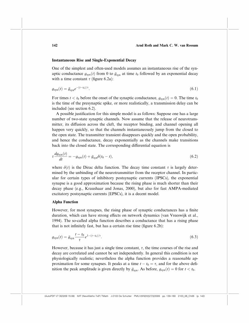
Instantaneous Rise and Single-Exponential Decay

One of the simplest and often-used models assumes an instantaneous rise of the syn-

aptic conductance gsynðtÞ from 0 to gsyn at time t0 followed by an exponential decay

with a time constant t (figure 6.2a):

gsynðtÞ ¼ gsyne�ðt�t0Þ=t: ð6:1Þ

For times t < t0 before the onset of the synaptic conductance, gsynðtÞ ¼ 0. The time t0is the time of the presynaptic spike, or more realistically, a transmission delay can be

included (see section 6.2).

A possible justification for this simple model is as follows: Suppose one has a large

number of two-state synaptic channels. Now assume that the release of neurotrans-

mitter, its di¤usion across the cleft, the receptor binding, and channel opening all

happen very quickly, so that the channels instantaneously jump from the closed to

the open state. The transmitter transient disappears quickly and the open probability,

and hence the conductance, decay exponentially as the channels make transitions

back into the closed state. The corresponding di¤erential equation is

tdgsynðtÞ

dt¼ �gsynðtÞ þ gsyndðt0 � tÞ; ð6:2Þ

where dðtÞ is the Dirac delta function. The decay time constant t is largely deter-

mined by the unbinding of the neurotransmitter from the receptor channel. In partic-

ular for certain types of inhibitory postsynaptic currents (IPSCs), the exponential

synapse is a good approximation because the rising phase is much shorter than their

decay phase (e.g., Kraushaar and Jonas, 2000), but also for fast AMPA-mediated

excitatory postsynaptic currents (EPSCs), it is a decent model.

Alpha Function

However, for most synapses, the rising phase of synaptic conductances has a finite

duration, which can have strong e¤ects on network dynamics (van Vreeswijk et al.,

1994). The so-called alpha function describes a conductance that has a rising phase

that is not infinitely fast, but has a certain rise time (figure 6.2b):

gsynðtÞ ¼ gsynt� t0

te1�ðt�t0Þ=t: ð6:3Þ

However, because it has just a single time constant, t, the time courses of the rise and

decay are correlated and cannot be set independently. In general this condition is not

physiologically realistic; nevertheless the alpha function provides a reasonable ap-

proximation for some synapses. It peaks at a time t� t0 ¼ t, and for the above defi-

nition the peak amplitude is given directly by gsyn. As before, gsynðtÞ ¼ 0 for t < t0.



Di¤erence of Two Exponentials

A more general function describing synaptic conductance profiles consists of a sum

of two exponentials, one for the rising and one for the decay phase. It allows these

time constants to be set independently ðtrise 0 tdecayÞ, so that for tb t0 (figure 6.2c):

gsynðtÞ ¼ gsyn f ðe�ðt�t0Þ=tdecay � e�ðt�t0Þ=triseÞ: ð6:4Þ

The normalization factor f is included to ensure that the amplitude equals gsyn. The

conductance peaks at a time:

tpeak ¼ t0 þtdecaytrise

tdecay � triseln

tdecay

trise

� �; ð6:5Þ

and the normalization factor for the amplitude follows as

f ¼ 1

�e�ðtpeak�t0Þ=trise þ e�ðtpeak�t0Þ=tdecay: ð6:6Þ

In the case of most synapses, rapid binding is followed by slow unbinding of the

transmitter. This particular profile of the synaptic conductance can be interpreted as

the solution of two coupled linear di¤erential equations (Wilson and Bower, 1989;

Destexhe et al. 1994):

gsynðtÞ ¼ gsyn fgðtÞ ð6:7Þ

dg

dt¼ � g

tdecayþ h ð6:8Þ

dh

dt¼ � h

triseþ h0dðt0 � tÞ; ð6:9Þ

with h0 a scaling factor. The alpha function is retrieved in the limit when both time

constants are equal.

The time course of most synaptic conductances can be well described by this sum

of two exponentials. It is of course possible to further increase the number of expo-

nentials describing the synaptic conductance to obtain even better fits, but then no

closed-form expression for the time of peak and the normalization factor for the am-

plitude exists. Furthermore, extracting a large number of exponentials from noisy

data is cumbersome (see later discussion).

Conductance-Based and Current-Based Synapses

Most ligand-gated ion channels mediating synaptic transmission, such as AMPA-

type glutamate receptors and g-aminobutryic acid type A (GABAA) receptors (see

Modeling Synapses 143


section 6.3), display an approximately linear current-voltage relationship when they

open. They can therefore be modeled as an ohmic conductance gsyn which when mul-

tiplied with the driving force, the di¤erence between the membrane potential V and

the reversal potential Esyn of the synaptic conductance, gives the synaptic current

Isyn ¼ gsynðtÞ½VðtÞ � Esyn�: ð6:10Þ

However, in some cases, in particular in analytical models, it may be a useful ap-

proximation to consider synapses as sources of current and not a conductance, i.e.,

without the dependence on the membrane potential V as described by equation

(6.10). This can be achieved, for example, by using a fixed value V ¼ Vrest in equa-

tion (6.10). For small excitatory synapses on a large compartment, this is a good ap-

proximation. In that case, the depolarization of the membrane will be small and

hence the di¤erence between V and Esyn will hardly change during the excitatory

postsynaptic potential (EPSP). However, if the synapse is located on a thin dendrite,

the local membrane potential V changes considerably when the synapse is activated

(Nevian et al., 2007). In that case a conductance-based synapse model seems more

appropriate. Nevertheless, voltage-dependent ion channels in the dendritic mem-

brane, together with a voltage-dependent component in the synaptic conductance g,

mediated by NMDA receptors (see next), can at least partially compensate for the

change in membrane potential and can cause synapses to e¤ectively operate as cur-

rent sources (Cook and Johnston, 1999).

For inhibitory synapses, the distinction between conductance-based and current-

based models is particularly important because the inhibitory reversal potential can

be close or even above the resting potential. As a result, the resulting synaptic current

becomes highly dependent on the postsynaptic voltage. This shunting leads to short-

ening of the membrane time constant, which does not occur for current-based mod-

els. This can have substantial consequences for network simulations (Koch, 1999;

Vogels and Abbott, 2005; Kumar et al., 2008; chapter 13, section 7).

Simple Descriptions of NMDA Receptor-Mediated Synaptic Conductances

Excitatory synaptic currents commonly have both AMPA and NMDA components.

The NMDA current is mediated by NMDA channels, which like AMPA channels,

are activated by glutamate but have a di¤erent sensitivity. The NMDA receptor-

mediated conductance depends on the postsynaptic voltage, i.e., equation (6.10) is

not valid. The voltage dependence is due to the blocking of the pore of the NMDA

receptor from the outside by a positively charged magnesium ion. The channel is

nearly completely blocked at resting potential, but the magnesium block is relieved

if the cell is depolarized. The fraction of channels uðVÞ that are not blocked by mag-

nesium can be fitted to



uðVÞ ¼ 1

1þ e�aV ½Mg2þ�o=b; ð6:11Þ

with a ¼ 0:062 mV�1 and b ¼ 3:57 mM (Jahr and Stevens, 1990). Here ½Mg2þ�o is

the extracellular magnesium concentration, usually 1 mM. If we make the approxi-

mation that the magnesium block changes instantaneously with voltage and is inde-

pendent of the gating of the channel, the net NMDA receptor-mediated synaptic

current is given by

INMDA ¼ gNMDAðtÞuðVÞ½VðtÞ � ENMDA�; ð6:12Þ

where gNMDAðtÞ could for instance be modeled by a di¤erence of exponentials, equa-

tion (6.4). Thus NMDA receptor activation requires both presynaptic activity (to

provide glutamate) and postsynaptic activity (to release the magnesium block). This

property has wide implications for the functional role of NMDA receptors for synap-

tic integration (Schiller et al., 2000; Losonczy and Magee, 2006; Nevian et al., 2007),

neuronal excitability (Rhodes and Llinas, 2001), network dynamics (Compte, 2006;

Durstewitz and Seamans, 2006; Durstewitz and Gabriel, 2007) and synaptic plastic-

ity (Bliss and Collingridge, 1993).

Finally, NMDA receptors have a significant permeability for calcium ions and

constitute one of the pathways for calcium entry, which is relevant for synaptic plas-

ticity (Nevian and Sakmann, 2006). To calculate the calcium current through the

NMDA receptor, the Goldman-Hodgkin-Katz equation should be used (see equa-

tion 4.2 and Badoual et al., 2006).

Synaptic Time Constants for AMPA, NMDA, and GABAA

The time constants of synaptic conductances vary widely among synapse types.

However, some general trends and typical values can be identified. First, synaptic ki-

netics tends to accelerate during development (T. Takahashi, 2005). Second, synaptic

kinetics becomes substantially faster with increasing temperature. In the following

discussion, we therefore focus on data from experiments performed at near-

physiological temperature (34–38 �C). This is important because the temperature de-

pendence is di¤erent for the various processes involved in synaptic transmission

(transmitter di¤usion, receptor kinetics, single channel conductance, etc.). In analogy

with voltage-gated channels, the temperature dependence can be approximated with

a Q10 factor, which describes the speedup with every 10 degrees of temperature in-

crease (equation 5.43). In particular, the temperature dependence of synaptic kinetics

is generally steep, with a Q10 of typically around 2–3 (Huntsman and Huguenard,

2000; Postlethwaite et al., 2007). Further complication arises because the Q10 of the

di¤erent transitions in the state diagram can vary (e.g., Cais et al., 2008), so that a

uniform scaling of all time constants is not appropriate.



AMPA receptor-mediated EPSCs at glutamatergic synapses are among the fastest

synaptic currents, but because di¤erent types of neurons express di¤erent subtypes of

AMPA receptors (see section 6.3), a range of time constants is observed. The fastest

AMPA receptor-mediated EPSCs are found in the auditory system where tdecay ¼0:18 ms in the chick nucleus magnocellularis (Trussell, 1999). Excitatory synapses

onto interneurons in the cortex and hippocampus also tend to have a fast AMPA

component (trise ¼ 0:25 ms and tdecay ¼ 0:77 ms in dentate gyrus basket cells; Geiger

et al., 1997). Synapses onto pyramidal neurons tend to have slower AMPA compo-

nents (trise ¼ 0:2 ms and tdecay ¼ 1:7 ms in neocortical layer 5 pyramidal neurons;

Hausser and Roth, 1997b).

The NMDA receptor-mediated component of the EPSC is typically more than an

order of magnitude slower than the AMPA receptor-mediated component. The slow

unbinding rate of glutamate from the NMDA receptor makes NMDA more sensitive

to glutamate and causes glutamate to stick longer to the receptor, increasing the open

time. The decay time constants at near-physiological temperature range from 19 ms

in dentate gyrus basket cells (Geiger et al., 1997) to 26 ms in neocortical layer 2/3

pyramidal neurons (Feldmeyer et al., 2002), and up to 89 ms in CA1 pyramidal cells

(Diamond, 2001). Likewise NMDA rise times, which are about 2 ms (Feldmeyer et

al., 2002), are slower than AMPA rise times. The reversal potential of both AMPA

and NMDA receptor-mediated currents is, conveniently, around 0 mV under physi-

ological conditions.

Synapses often contain both AMPA and NMDA receptor-mediated conductances

in a specific ratio (Feldmeyer et al., 2002; Losonczy and Magee, 2006). However,

there are also NMDA receptor-only synapses, so-called silent synapses (Liao et al.,

1995; Isaac et al., 1995; Groc et al., 2006). These have little or no synaptic current

at the resting potential because the NMDA receptors are blocked by magnesium.

A few types of synapses are AMPA receptor-only synapses during development

(Cathala et al., 2000; Clark and Cull-Candy, 2002).

GABAA receptor-mediated IPSCs tend to decay more slowly than the AMPA con-

ductances. GABAergic synapses from dentate gyrus basket cells onto other basket

cells are faster: trise ¼ 0:3 ms and tdecay ¼ 2:5 ms (Bartos et al., 2001) than synapses

from basket cells to granule cells: trise ¼ 0:26 ms and tdecay ¼ 6:5 ms (Kraushaar and

Jonas, 2000). Reversal potentials of GABAA receptor-mediated conductances change

with development (Ben-Ari, 2002) and activity (Fiumelli and Woodin, 2007).

Experimentally, accurate measurement of synaptic currents and time constants is

di‰cult because the voltage in dendrites is di‰cult to control (known as the space-

clamp problem; chapter 10, section 3), leading to an overestimate of the rise and de-

cay time constants of the synaptic conductance at distal dendritic locations. Care

should therefore be taken to minimize this by optimizing recording conditions,

recording from small (i.e., electrically compact) cells, or employing analysis tech-



niques that provide an unbiased estimate of the decay time constant of the synaptic

conductance (Hausser and Roth, 1997b; Williams and Mitchell, 2008).

6.2 Implementation Issues

Given the large number of synapses in most network simulations, e‰cient simulation

of synapses is key. For home-brewed simulations, an easy trick is the following:

Whereas updating all the synaptic conductances at every time step according to, for

instance equation (6.1), is computationally costly, if the postsynaptic neuron contains

just a single compartment (e.g., an integrate-and-fire neuron, chapter 7), all synaptic

conductances with identical parameters can be lumped together into a total synaptic

conductance (Lytton, 1996). This total synaptic conductance gS increases when any

of the synapses onto the neuron are activated, i.e., gS ¼ gS þ gi, where i sums over

the activated synapses. Only the decay of this summed conductance has to be calcu-

lated at each time step dt. For instance, in the case of a single exponential decay,

gSðtþ dtÞ ¼ gSðtÞ expð�dt=tÞ, meaning that the computational cost of updating the

synaptic conductance is on the order of the number of neurons; i.e., it is comparable

to the cost of updating the neuron’s membrane potentials only.

Implementation in Simulator Packages

Models of synaptic transmission have also been implemented in neural simulation

packages (see the software appendix). Work is under way to improve the accuracy

and e‰ciency of these implementations and, depending on the application, di¤erent

simulation strategies may be the most accurate and most e‰cient (Brette et al.,

2007). One strategy is to compute the synaptic conductance time courses as the solu-

tions of the corresponding linear di¤erential equations, which can be integrated nu-

merically using discrete time steps, or in some cases can be solved analytically

(Destexhe et al., 1998a; Rotter and Diesmann, 1999; Carnevale and Press, 2006). In-

stead of analytical solutions, precomputed lookup tables for the synaptic and neuro-

nal dynamics can be also used (Ros et al., 2006).

Another approach is to use event-driven methods, which are particularly e‰cient

in cases that allow an analytical solution for the response of the postsynaptic neuron

(Brette, 2006; Carnevale and Hires, 2006; Rudolph and Destexhe, 2006; chapter 7).

These algorithms extrapolate the time at which neuron will spike, removing the need

for simulating the intermediate time steps. However, if input rates are high, these

extrapolations have to be revised frequently, nullifying their benefit. Finally, hybrid

strategies that combine time-driven and event-driven methods are available (Morri-

son et al., 2007). Most synapse models discussed here have also been implemented

in hardware, both using analog very large-scale integration (VLSI) (Rasche and



Douglas, 1999; Mira and Alvarez, 2003; Zou et al., 2006; Bartolozzi and Indiveri,

2007) and field-programmable gate arrays (FPGAs) (Guerrero-Rivera et al., 2006).

Axonal, Synaptic, and Dendritic Delays

The postsynaptic response to a presynaptic spike is not instantaneous. Instead, axo-

nal, synaptic, and dendritic delays all contribute to the onset latency of the synaptic

current with respect to the time of the presynaptic spike. Since these delays can add

up to several milliseconds and thus can be comparable in duration to the synaptic

time constant, they can have consequences for synchronization and oscillations (Bru-

nel and Wang, 2003; Maex and De Schutter, 2003; chapter 13, section 3) and the sta-

bility of spike timing-dependent plasticity (STDP) in recurrent networks (Morrison et

al., 2007). In practice, long delays benefit parallel simulation algorithms (chapter 13,

section 6).

6.3 Biophysics of Synaptic Transmission and Synaptic Receptors

After describing these simplified models of synapses, we now focus on the underlying

mechanisms of synaptic transmission, which will allow discussion of the more realis-

tic models presented in section 6.4. The precise shape of synaptic events is deter-

mined by the biophysical mechanisms that underlie synaptic transmission. Numerous

in-depth reviews of synaptic physiology and kinetic models of synaptic receptor mol-

ecules exist (Jonas and Spruston, 1994; Jonas, 2000; Attwell and Gibb, 2005; Lisman

et al., 2007).

Transmitter Release

The signaling cascade underlying synaptic transmission (figure 6.1) begins with the

arrival of the presynaptic action potential in the presynaptic terminal, where it acti-

vates various types of voltage-gated ion channels (Meir et al., 1999), in particular,

voltage-gated calcium channels. The calcium current through these channels reaches

its maximum during the repolarization phase of the action potential as the driving

force for calcium ions increases while the calcium channels begin to deactivate (Borst

and Sakmann, 1998). This calcium influx leads to a local increase in the intracellular

calcium concentration (see chapter 4, section 3 and section 6.5), which in turn trig-

gers the release of neurotransmitter molecules from vesicles, owing either to their

full fusion with the presynaptic membrane or the formation of a fusion pore (He et

al., 2006).

Transmitter Di¤usion

Following its release, the neurotransmitter di¤uses in the synaptic cleft. The spatio-

temporal profile of transmitter concentration in the synaptic cleft depends on a num-



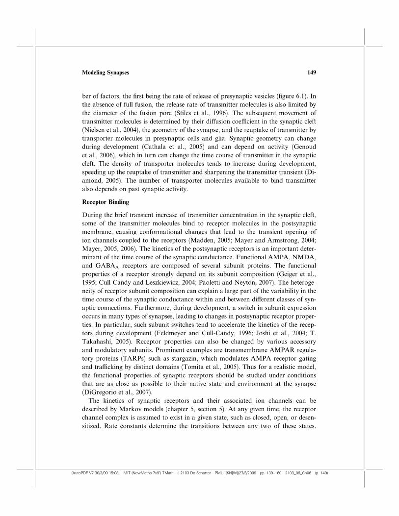
ber of factors, the first being the rate of release of presynaptic vesicles (figure 6.1). In

the absence of full fusion, the release rate of transmitter molecules is also limited by

the diameter of the fusion pore (Stiles et al., 1996). The subsequent movement of

transmitter molecules is determined by their di¤usion coe‰cient in the synaptic cleft

(Nielsen et al., 2004), the geometry of the synapse, and the reuptake of transmitter by

transporter molecules in presynaptic cells and glia. Synaptic geometry can change

during development (Cathala et al., 2005) and can depend on activity (Genoud

et al., 2006), which in turn can change the time course of transmitter in the synaptic

cleft. The density of transporter molecules tends to increase during development,

speeding up the reuptake of transmitter and sharpening the transmitter transient (Di-

amond, 2005). The number of transporter molecules available to bind transmitter

also depends on past synaptic activity.

Receptor Binding

During the brief transient increase of transmitter concentration in the synaptic cleft,

some of the transmitter molecules bind to receptor molecules in the postsynaptic

membrane, causing conformational changes that lead to the transient opening of

ion channels coupled to the receptors (Madden, 2005; Mayer and Armstrong, 2004;

Mayer, 2005, 2006). The kinetics of the postsynaptic receptors is an important deter-

minant of the time course of the synaptic conductance. Functional AMPA, NMDA,

and GABAA receptors are composed of several subunit proteins. The functional

properties of a receptor strongly depend on its subunit composition (Geiger et al.,

1995; Cull-Candy and Leszkiewicz, 2004; Paoletti and Neyton, 2007). The heteroge-

neity of receptor subunit composition can explain a large part of the variability in the

time course of the synaptic conductance within and between di¤erent classes of syn-

aptic connections. Furthermore, during development, a switch in subunit expression

occurs in many types of synapses, leading to changes in postsynaptic receptor proper-

ties. In particular, such subunit switches tend to accelerate the kinetics of the recep-

tors during development (Feldmeyer and Cull-Candy, 1996; Joshi et al., 2004; T.

Takahashi, 2005). Receptor properties can also be changed by various accessory

and modulatory subunits. Prominent examples are transmembrane AMPAR regula-

tory proteins (TARPs) such as stargazin, which modulates AMPA receptor gating

and tra‰cking by distinct domains (Tomita et al., 2005). Thus for a realistic model,

the functional properties of synaptic receptors should be studied under conditions

that are as close as possible to their native state and environment at the synapse

(DiGregorio et al., 2007).

The kinetics of synaptic receptors and their associated ion channels can be

described by Markov models (chapter 5, section 5). At any given time, the receptor

channel complex is assumed to exist in a given state, such as closed, open, or desen-

sitized. Rate constants determine the transitions between any two of these states.



State transitions involving the binding of a transmitter molecule to the receptor are

described by rate constants that are proportional to the transmitter concentration.

The rate constants are free parameters in these models, which need to be extracted

from experimental data. Except for the simplest Markov models with only two or

three states, which might not describe the synaptic receptors very well, the number

of rate constants and thus the number of free parameters is significantly larger than

the number of free parameters in simple functions describing synaptic conductance

kinetics (section 6.1). It is usually necessary to expose receptors to a number of pro-

tocols involving both short and long pulses of transmitter concentration (e.g.,

Hausser and Roth, 1997a) to adequately constrain a Markov model of their kinetics.

A number of Markov models for AMPA receptors from di¤erent types of neurons

have been obtained in this way (Nielsen et al., 2004). Figure 6.3a shows a kinetic

model of synaptic AMPA receptors in cerebellar granule cells (DiGregorio et al.,

2007) and table 6.1 provides the rate constants for the models. Kinetic models of

NMDA receptors with a slow component of the magnesium unblock (Kampa et al.,

2004; Vargas-Caballero and Robinson, 2003, 2004; figure 6.3c) can be useful for sim-

ulations of NMDA receptor-dependent synaptic plasticity (section 6.7).

In order to use Markov models of synaptic receptors, a model of the time course

of the transmitter concentration in the synaptic cleft is needed to drive the Markov

model. Models of transmitter di¤usion in detailed synaptic geometries (section 6.5)

may provide fairly accurate predictions of the time course of transmitter concen-

tration, but are computationally very expensive. However, because the transmitter

Figure 6.3Kinetic schemes for common synaptic channels. Closed states are denoted with a C, open states with an O,and desensitized states with a D. Primes are used to distinguish otherwise identical states. The transmitteris denoted by T. A circled state denotes the state at rest, in the absence of a transmitter. (a) AMPA recep-tor kinetic model after DiGregorio et al. (2007). Two transmitter molecules T need to bind for the channelto open. (b) GABAA receptor kinetic model after Pugh and Raman (2005). Note that there are two openstates in this case. The desensitized states are split into slow (sD) and fast (fD) ones. (c) NMDA receptorkinetic model after Kampa et al. (2004). The model includes the kinetics of magnesium (Mg) binding. Forsimplicity, the binding with both glutamate molecules has been captured in a single transition. Again thereare both slow and fast desensitized states.



Table 6.1Rate constants for the models in figure 6.3

Transition Forward Backward

AMPA

C-CT 13.66 mM�1ms�1 8.16 ms�1

CT-CT2 6.02 mM�1ms�1 4.72 ms�1

CT-C 0T 0.11 ms�1 0.1 ms�1

C 0T-C 0T2 13.7 mM�1ms�1 1.05 ms�1

C 0T2-C00T2 0.48 ms�1 0.98 ms�1

CT2-OT2 17.2 ms�1 3.73 ms�1

C 00T2-D0T2 10.34 ms�1 4 ms�1

CT2-C0T2 2 ms�1 0.19 ms�1

OT2-C00T2 0.0031 ms�1 0.0028 ms�1

OT2-DT2 0.11 ms�1 0.09 ms�1

DT2-D0T2 0.0030 ms�1 0.0013 ms�1

GABAA

C-CT 0.04 mM�1ms�1 2 ms�1

CT-OT 0.03 ms�1 0.06 ms�1

CT-DT 0.000333 ms�1 0.0007 ms�1

CT-CT2 0.02 mM�1ms�1 4 ms�1

CT2-OT 10 ms�1 0.4 ms�1

CT2-sDT2 1.2 ms�1 0.006 ms�1

CT2-fDT2 15 ms�1 0.15 ms�1

DT-sDT2 0.015 mM�1ms�1 0.007 ms�1

NMDAa

C-CT2 10 mM�1s�1 5.6 s�1

CMg-CMgT2 10 mM�1s�1 17.1 s�1

CT2-OT2 10 s�1 273 s�1

CMgT2-OMgT2 10 s�1 548 s�1

CT2-fDT2 2.2 s�1 1.6 s�1

CMgT2-fDMgT2 2.1 s�1 0.87 s�1

fDT2-sDT2 0.43 s�1 0.50 s�1

fDMgT2-sDMgT2 0.26 s�1 0.42 s�1

O-OMg (at þ40 mV) 0.05 mM�1s�1 12,800 s�1

x-xMg (at þ40 mV) 50.10�6 mM�1s�1 12.8 s�1

aSee also http://senselab.med.yale.edu/modeldb, model ¼ 50207.



transient is much faster than the receptor dynamics, a brief square pulse or a

single-exponential decay su‰ces (Destexhe et al., 1998a).

Second-Messenger Synapses

In the preceding discussion, the transmitter binds to the ion channels directly,

so-called ionotropic receptors. However, this is not always the case. In second-

messenger or metabotropic receptors (Coutinho and Knopfel, 2002), the neurotrans-

mitter binds to a receptor that activates an intermediate G-protein, which in turns

binds to a G-protein-gated ion channel and opens it. As a result of the intermediate

cascade, the synaptic responses of second-messenger synapses are usually slower, but

they can also be very sensitive and highly nonlinear. For the same reason, unified

models of second-messenger synapses are rare and can display a rich behavior. The

best-known examples of these synapses are the metabotropic glutamate receptors

and the inhibitory receptor GABAB. In the case of GABAB, the inhibitory current

becomes disproportionally stronger with multiple events (Destexhe et al., 1998a).

The nonlinearity of the mGluR receptor in retinal bipolar cells has, for instance,

been proposed to filter out photoreceptor noise (van Rossum and Smith, 1998). Fi-

nally, mGluR receptors have also been found presynaptically (T. Takahashi et al.,

1996; R. J. Miller, 1998).

6.4 Modeling Dynamic Synapses

Many of the biophysical mechanisms involved in synaptic transmission are use depen-

dent (Zucker and Regehr, 2002). For example, residual elevations of the presynap-

tic calcium concentration that are due to a previous action potential can increase

the probability of subsequent transmitter release. An increase in the synaptic re-

sponse to successive stimuli is called synaptic facilitation. On the other hand, deple-

tion of the pool of readily releasable vesicles can cause a decrease of the synaptic

response to successive stimuli, called short-term synaptic depression (to distinguish

it from long-term synaptic depression, LTD, the counterpart of long-term potentia-

tion, LTP). Depression and facilitation of synaptic currents can also have postsynap-

tic components. Cumulative desensitization of postsynaptic receptors can contribute

to synaptic depression, while increased occupancy of transporters can lead to a pro-

longed presence of transmitter molecules in the synaptic cleft and a facilitation of

synaptic responses.

Short-term synaptic plasticity is a major determinant of network dynamics. It can

provide gain control, underlie adaptation and detection of transients, and constitute

a form of short-term memory (Abbott and Regehr, 2004; chapter 13, section 3). The

characteristics of short-term synaptic plasticity depend on (and can be used to define)

the type of synaptic connection in a neural circuit (Silberberg et al., 2005). A number



of functional consequences of short synaptic dynamics have been suggested: tempo-

ral filtering (Puccini et al., 2007), gain adaptation (Abbott et al., 1997), decorrelation

of inputs (Goldman et al., 2002), working memory (Mongillo et al., 2008), and adap-

tive visual processing (van Rossum et al., 2008).

The amplitude and time constants of synaptic depression and facilitation, which

can be determined experimentally using trains of synaptic stimuli, are free parame-

ters of simple phenomenological models of short-term synaptic plasticity (Abbott et

al., 1997; Markram et al., 1998; Tsodyks et al., 2000). These models are a good ap-

proximation of the short-term dynamics of many types of synapses and can be imple-

mented e‰ciently.

We present here the model of Tsodyks and Markram as described in Tsodyks et al.

(1998, 2000). In this model, the ‘‘resources’’ of the synapse that provide the synaptic

current or conductance can exist in one of three states: the recovered or resting state,

with occupancy x; the active or conducting state, y; and an inactive state, z. At any

given time

xþ yþ z ¼ 1: ð6:13Þ

A fourth state variable, u, describes the ‘‘use’’ of synaptic resources in response to a

presynaptic action potential arriving at time t ¼ t0. Its dynamics is given by

du

dt¼ � u

tfacilþUð1� uÞdðt� t0Þ; ð6:14Þ

so u is increased by Uð1� uÞ with each action potential and decays back to zero with

a time constant tfacil. This u drives the dynamics of the other three state variables

according to

dx

dt¼ z

trec� uxdðt� t0Þ ð6:15Þ

dy

dt¼ � y

tdecayþ uxdðt� t0Þ ð6:16Þ

dz

dt¼ y

tdecay� z

trec; ð6:17Þ

where trec is the time constant of recovery from depression and tdecay (corresponding

to t in equation 6.1) is the time constant of decay of the synaptic current or conduc-

tance, which is proportional to y.

Typical observed time constants for recovery are between 100 and 1,000 ms in

vitro. The time constants and magnitude of synaptic depression in vivo have not

been clearly established, however. With background activity, synapses might already



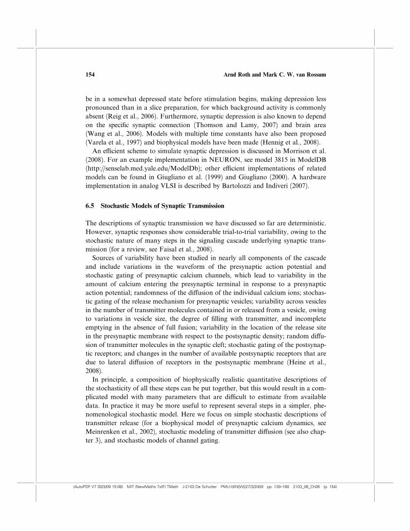
be in a somewhat depressed state before stimulation begins, making depression less

pronounced than in a slice preparation, for which background activity is commonly

absent (Reig et al., 2006). Furthermore, synaptic depression is also known to depend

on the specific synaptic connection (Thomson and Lamy, 2007) and brain area

(Wang et al., 2006). Models with multiple time constants have also been proposed

(Varela et al., 1997) and biophysical models have been made (Hennig et al., 2008).

An e‰cient scheme to simulate synaptic depression is discussed in Morrison et al.

(2008). For an example implementation in NEURON, see model 3815 in ModelDB

(http://senselab.med.yale.edu/ModelDb); other e‰cient implementations of related

models can be found in Giugliano et al. (1999) and Giugliano (2000). A hardware

implementation in analog VLSI is described by Bartolozzi and Indiveri (2007).

6.5 Stochastic Models of Synaptic Transmission

The descriptions of synaptic transmission we have discussed so far are deterministic.

However, synaptic responses show considerable trial-to-trial variability, owing to the

stochastic nature of many steps in the signaling cascade underlying synaptic trans-

mission (for a review, see Faisal et al., 2008).

Sources of variability have been studied in nearly all components of the cascade

and include variations in the waveform of the presynaptic action potential and

stochastic gating of presynaptic calcium channels, which lead to variability in the

amount of calcium entering the presynaptic terminal in response to a presynaptic

action potential; randomness of the di¤usion of the individual calcium ions; stochas-

tic gating of the release mechanism for presynaptic vesicles; variability across vesicles

in the number of transmitter molecules contained in or released from a vesicle, owing

to variations in vesicle size, the degree of filling with transmitter, and incomplete

emptying in the absence of full fusion; variability in the location of the release site

in the presynaptic membrane with respect to the postsynaptic density; random di¤u-

sion of transmitter molecules in the synaptic cleft; stochastic gating of the postsynap-

tic receptors; and changes in the number of available postsynaptic receptors that are

due to lateral di¤usion of receptors in the postsynaptic membrane (Heine et al.,

2008).

In principle, a composition of biophysically realistic quantitative descriptions of

the stochasticity of all these steps can be put together, but this would result in a com-

plicated model with many parameters that are di‰cult to estimate from available

data. In practice it may be more useful to represent several steps in a simpler, phe-

nomenological stochastic model. Here we focus on simple stochastic descriptions of

transmitter release (for a biophysical model of presynaptic calcium dynamics, see

Meinrenken et al., 2002), stochastic modeling of transmitter di¤usion (see also chap-

ter 3), and stochastic models of channel gating.



Stochastic Models of Vesicle Release

The description of synaptic potentials and synaptic currents as a sum of probabilisti-

cally generated ‘‘quantal components’’ has its origin in the work of del Castillo and

Katz (1954) at the neuromuscular junction. More recently, it has been used to inter-

pret the fluctuations of EPSP amplitudes measured in paired recordings from synap-

tically connected neurons in the central nervous system (Thomson et al., 1993;

Markram et al., 1997; Bremaud et al., 2007). In its simplest version, the synapse is

described as an arrangement of n independent release sites, each of which releases a

quantum of transmitter with a probability p in response to a presynaptic action po-

tential. Each released quantum of transmitter generates a contribution of size q to the

postsynaptic response r (which can be a synaptic conductance, current, or postsynap-

tic potential amplitude). Therefore r follows a binomial distribution and the mean re-

sponse hri is

hri ¼ npq: ð6:18Þ

Individual responses can be simulated using binomially distributed random numbers.

If n is low, this can be done by generating n random deviates uniformly distributed

between zero and one. The number of deviates smaller than p gives the synaptic am-

plitude after multiplication by q. By using di¤erent values of pi and qi, this scheme

can be generalized to the case that di¤erent release sites (indexed by i) have di¤erent

release probabilities pi and quantal sizes qi.

Typical values for p are between 0.1 and 0.5 but can vary widely, whereas n typi-

cally ranges between 3 and 20 (Markram et al. 1997; Bremaud et al., 2007). The

number of anatomical contacts is probably close to n, but because combining anat-

omy and physiology in a single experiment is di‰cult, a precise quantification is cur-

rently lacking.

For a model that combines stochastic release and short-term plasticity, see Maass

and Zador (1999). It is generally believed that the stochastic release of vesicles is a

large source of variability in the nervous system. Whether this variability is merely

the consequence of the underlying biophysics or has some functional role is a topic

of active debate.

Stochastic Models of Transmitter Di¤usion

A simulator for the stochastic simulation of transmitter di¤usion and receptor bind-

ing is MCell (see the software appendix). MCell simulates di¤usion of single mole-

cules and the reactions that take place as transmitter molecules bind to receptors

and transporters, which can be used to quantify the di¤erent sources of variability

(Franks et al., 2003; Raghavachari and Lisman, 2004).



Stochastic Models of Receptors

A stochastic description of the stochastic opening of the postsynaptic receptors is

straightforward once a Markov model has been formulated. Instead of using the av-

erage transition rates in the state diagram, at each time step the transitions from one

state to another are drawn from a binomial distribution, with a probability p equal

to the transition rate per time step, and n equal to the number of channels in the state

at which the transitions are made. The fewer receptors there are in the postsynaptic

membrane, the more pronounced the fluctuations around the average behavior will

be. The typical number of postsynaptic receptors is believed to be in the range of 10

to 100. Compared with the other sources of variability, the noise from stochastic

opening of the receptor channels is usually minor (van Rossum et al., 2003). Never-

theless, the fluctuations across trials can be used to determine the unitary conduc-

tance of the receptors using so called nonstationary noise analysis (Hille, 2001).

Computationally, these simulations are expensive because the number of transitions

is assumed to be small in the simulation, whereas the transition rates can be high,

necessitating a very small time step.

6.6 Modeling Synaptic Learning Rules

One of the central hypotheses in neuroscience is that learning and memory are

reflected in the weight of synapses. Many experiments and models have studied

therefore how synapses change in response to neural activity, so-called activity-

dependent synaptic plasticity. Some models have as their aim the construction of

learning rules so that the network performs a certain task, such as learning input-

output associations (for instance, using backpropagation), independent component

analysis, or achieving sparse codes. Because the links between these models and the

physiology are often tentative, we will not describe them here. Another class of mod-

els, discussed here, uses a phenomenological approach and implements biologically

observed learning rules to examine their functional consequences.

The biological pathways underlying synaptic plasticity are only just starting to be

understood, but it clear that they contain many ingredients and regulation mecha-

nisms. Although e¤orts are being made to model at this level (chapter 3), for network

studies one often prefers a simpler model. This separation of levels of complexity is

often desirable conceptually, but also from a computational perspective. In plasticity

studies one is often interested in a network’s properties as they evolve over longer

periods of time or when many stimuli are presented. This means that simulation

studies of learning are computationally particularly expensive and require e‰cient

algorithms.



The fundamental experimental finding is that brief exposure to high pre- and post-

synaptic activity causes long-lasting increases in synaptic strength, which can persist

up to months in vivo (Bliss and Lomo, 1973). This finding is consistent with Hebb’s

hypothesis (Hebb, 1949) and is called Hebbian learning. This phenomenon is known

as LTP. Similarly low, but nonzero, levels of activity can cause long-lasting weaken-

ing of synapses, LTD. Consistent with most experiments, increases and decreases in

synaptic e‰cacy in most models are implemented through changes in the postsynap-

tic conductance gsyn, although in some studies evidence for changes in the release

probability was found and has been included in models (Tsodyks and Markram,

1997; Maass and Zador, 1999).

Rate-Based Plasticity

In an e¤ort to condense the experimental data on plasticity, early plasticity models

used often a rate-based formulation, which, for instance, takes the form (Sejnowski,

1977):

Dwij ¼ eðri � aÞðrj � bÞ; ð6:19Þ

where ri is the presynaptic firing rate, rj is the postsynaptic firing rate, wij is the syn-

aptic weight connecting the neurons, and a and b are constants. Finally, the propor-

tionality constant e is often taken to be a small number, ensuring that the synaptic

weights change only slowly. The rates are assumed to be averaged over times longer

than any single neuron dynamics (such as spikes) but shorter than the stimulus

dynamics. Such a learning rule, for instance, can be used to train networks receiving

sensory input in an unsupervised manner.

It is not di‰cult to see that this learning rule diverges, however, because once a

synapse becomes stronger, it will evoke a higher postsynaptic activity, which leads

to a further increase in its strength, etc. A variety of solutions have been proposed

to deal with this problem. These include imposing maximum and minimum weights,

normalizing the sum of all the weights coming into a neuron, while the Bienenstock-

Cooper-Munro (BCM) rule adjusts the thresholds of LTP and LTD as a function of

average postsynaptic activity (Bienenstock et al. 1982; Dayan and Abbott, 2002).

The precise solution strongly a¤ects the resulting behavior of the learning rule while

at the same time experimental data on this issue are largely lacking. Despite this un-

certainty, or maybe owing to the freedom it allowed, many rate-based plasticity

models have been used successfully to describe memory models (Bienenstock et al.,

1982; K. D. Miller, 1996; Miikkulainen and Sirosh, 2005).

Spike Timing-Dependent Plasticity

Changes in synaptic weight depend not only on mean firing rates but also on the pre-

cise temporal order of pre- and postsynaptic spikes, a phenomenon known as STDP



(Abbott and Gerstner, 2004). Given a spike at time ti in the presynaptic neuron and

at time tj in the postsynaptic neuron, a simple description of STDP is

Dwij ¼ e signðti � tjÞ expð�jti � tjj=tSTDPÞ; ð6:20Þ

where tSTDP is the time window for spike pair interaction, some 20 ms. Note that the

weight change is discontinuous when ti ¼ tj.

However, the apparent simplicity of the STDP rule is a bit misleading because for

an actual implementation, additional specifications are needed. First, without any

further constraints, weights will diverge as more and more spike pairs are encoun-

tered. As for rate-based plasticity rules, bounds can be imposed. These can be hard

bounds that simply cap the maximal weight, or softer bounds that, for instance, re-

duce the amount of potentiation as the weight increases. In addition, homeostatic

mechanisms can be included that modify the learning rules based on the total post-

synaptic activity. Second, one needs to define which spike pairs contribute to weight

changes. For instance, what happens if a presynaptic spike is followed by two post-

synaptic spikes; do both contribute to a weight modification? Such rules can be clas-

sified and analyzed formally to some extent (Burkitt et al., 2004).

Although in equation (6.20) the STDP rule is independent of the pre- and post-

synaptic rate, experiments show that higher pairing frequencies usually cause LTP

and lower frequencies cause LTD. As long as there is no experimental evidence that

STDP and rate-based learning are separate plasticity mechanisms, it is convenient to

unify them in a single framework. Unified models of STDP and rate-based learning

that even include BCM-like plasticity have been created by allowing higher-order

interactions between spikes (Pfister and Gerstner, 2006).

This raises the question of whether the temporal character of STDP matters at all

or is simply a side e¤ect of a biological implementation of rate-based learning. Al-

though this issue has not been settled yet, there is evidence that some perceptual

learning shares properties with STDP (Dan and Poo, 2006) and that some plasticity

phenomena can only be explained by using STDP (Young et al., 2007).

Analysis of STDP in networks is in general di‰cult because of the mutual interac-

tion between the spike patterns in the network, which will modify the synapses, and

the plasticity, which will modify the activity patterns. Even creating a stable asyn-

chronous state in a network with STDP is challenging but possible (Morrison et al.,

2007).

Biophysical Models of Long-Term Potentiation

The molecular biology of LTP is quite complicated and involves numerous path-

ways. LTP is critically dependent on calcium influx in the postsynaptic membrane

that activates CaMKII (Lisman et al., 2002). The calcium influx is strongly depen-



dent on spike sequence and has been used as a basis for STDP (Shouval et al., 2002;

Badoual et al., 2006). Experiments have further distinguished between di¤erent

phases of plasticity, so-called early LTP (lasting a few hours) and late LTP (perhaps

lasting indefinitely). In particular, the stability of LTP has received attention from

modelers (Graupner and Brunel, 2007; Lisman and Raghavachari, 2006).

Again, synapses of di¤erent neurons obey di¤erent learning rules and even on a

given neuron, synapses at di¤erent dendritic locations can have distinct plasticity

rules (Sjostrom et al., 2008). Thus far this level of complexity has largely been

ignored in functional models.

6.9 Conclusions

We have presented synaptic models at various levels of physiological detail and real-

ism. We started with some quite simple formulations that nevertheless provide decent

models for the synaptic current. Increases in computer speed and increased under-

standing of neural transmission have made more and more complex models possible.

The researcher will need to consider a tradeo¤ between complex models and simpler

models that may ignore subtleties. However, a simple heuristic model is not necessar-

ily inferior, because it might actually do a better job in describing the physiology

than a complicated model with incorrect parameters.

Unless biophysical mechanisms of synaptic transmission themselves are the subject

of study, mechanistic detail is usually not needed. Experimental data that constrain

all parameters of these phenomenological models, such as voltage-clamp recordings

of synaptic current waveforms, are more likely to be available than full experimental

characterizations of the functional properties of the molecules and the biophysical

mechanisms involved. Furthermore, complex models not only require more com-

puter time but also more time to set up, verify, tune, and analyze. An informed

choice of model will depend on the question that is being asked. No matter what

model is used, parameter values should be considered carefully. For instance, the

strong temperature dependence of gating kinetics implies that data recorded at

room temperature should not simply be plugged into an in vivo model.

Recent years have also seen increased understanding of issues such as long-term

and short-term synaptic plasticity, receptor di¤usion, and subunit composition, to

name but a few. Unfortunately for the modeler, the known diversity among synapses

and their properties has also increased. The number of variations in synaptic subunit

composition, modulation (not discussed here), and long- and short-term dynamics is

ever increasing, and there is no reason to expect a slowdown in this trend. The rules

that underlie this diversity are so far largely unknown, so intuition and exploration

are required from the modeler.




Documents

A Roth and MvR, Modeling Synapses. Chapter in Computational Modeling Methods for