Embed Size (px)
Citation preview
A Search for Solar Axions
with the MICROMEGAS Detector
in CAST
Vom Fachbereich Physik der
TECHNISCHEN UNIVERSITAT DARMSTADT
zur Erlangung des Gradeseines Doktors der Naturwissenchaften
(Dr. rer. nat.)
genehmigte Dissertation vonTheopisti Dafniaus Thessaloniki
Darmstadt 2005D17
Referent: Prof. Dr. D. H. H. HoffmannKorreferent: Prof. Dr. P. Braun-Munzinger
Tag der Einreichung: 11.04.2005Tag der Prufung: 29.06.2005
Zusammenfassung
Die experimentelle Suche nach Axionen wird unter anderem durch das sogenannte CP-Problem der starken Wechselwirkung motiviert: die Theorie sagt eine Verletzung der CP-Symmetrie fur die starke Wechselwirkung vorher, die bislang jedoch in keinem Experimentnachgewiesen werden konnte. Peccei und Quinn fuhrten eine neue Symmetrie ein, um dasProblem zu losen: eine Symmetrie, die mit einem neuen, fast masselosen Boson, namlichdem Axion, verknupft ist. Das Axion ist sehr faszinierend, wenn man die Anzahl undVielfalt der Anwendungen, die seine Existenz impliziert, betrachtet: neben der Tatsache,dass es eine elegante Losung des CP-Problems liefert, ist es einer der zwei uberlebendenKandidaten fur die ”Dunkle Materie”.
Kosmologie und Astrophysik geben bereits erste Einschrankungen der Eigenschaftender Axionen bezuglich ihrer Masse und ihrer Kopplung an Fermionen, Nukleonen und Pho-tonen. Beachtet man alle diese Beschrankungen, so bleibt nur noch ein kleines Fenster imMassenbereich von µeV bis zu einigen eV offen, in dem Axionen zu erwarten sind. MehrereExperimente nutzen den Primakoff- Effekt, um nach Axionen zu suchen. In diesem Prozesskann ein Axion in einem elektrischen oder magnetischen Feld aus einem Photon entstehenund umgekehrt besteht die Moglichkeit, dass ein Axion sich unter ahnlichen Bedingungenin ein Photon umwandelt.
Mehrere Methoden wurden entwickelt und in die Tat umgesetzt, um Axionen nach-zuweisen. Das CAST-Experiment ist eines der Helioskope. Es benutzt einen fast 10 mlangen Prototypmagneten, des im Aufbau befindlichen Large Hadron Collider (LHC) amEuropaischen Kernforschungszentrum CERN in Genf. Dieser Magnet erreicht ein mag-netisches Feld von 9 T. Er ist auf einem einem beweglichen Aufbau ahnlich einem as-tronomischen Teleskop montiert. Die Bewegung dieses Aufbaus erlaubt es, den Magnetenfur etwa 100 Minuten wahrend des Sonnenaufgangs auf die Sonne auszurichten. Fur diegleiche Zeit kann die Sonne auch bei Sonnenuntergang beobachtet werden. Jede gegenu-ber dem Untergrund erhohte Zahlrate, die nur wahrend der Sonnenbeobachtung auftritt,wird als ein Signal der zu Photonen umgewandelten Axionen interpretiert.
Der Energiebereich der nachzuweisenden Photonen liegt zwischen 1 keV und etwa10 keV und erfordert daher den Einsatz von Rontgendetektoren. Auf der dem Sonnenun-tergang zugewandten Seite des Teleskops wird als Detektor eine Zeitprojektionskam-mer (Time Projektion Chamber, TPC) vewendet. Fur die Beobachtungszeit wahrenddes Sonnenaufgangs steht der in dieser Arbeit beschriebene Mikromegas-Detektor undein Rontgenteleskop zur Verfugung. Das Rontgenteleskop, der Prototyp eines Rontgen-Spiegelteleskops der deutschen Rontgensatelliten-Mission ABRIXAS, das an einer derbeiden Magnetoffnungen installiert ist, fokussiert die von den Axionen produzierten Pho-tonen auf ein Charged Coupled Device (CCD).
An der anderen Magnetoffnung, die bei Sonnenaufgang Axionen beobachtet, befindetsich ein Micromegas-Detektor. Dabei handelt es sich um einen Gasdetektor der Mikro-streifen -Art mit sehr asymmetrischer Doppelstruktur. Zusammen mit der hohen Gran-ularitat (384 Streifen) hat der Detektor eine sehr gute Orts- und Energieauflosung. Einweiterer interessanter Punkt fur diese Anwendung ist die hohe erreichte Unterdruckung
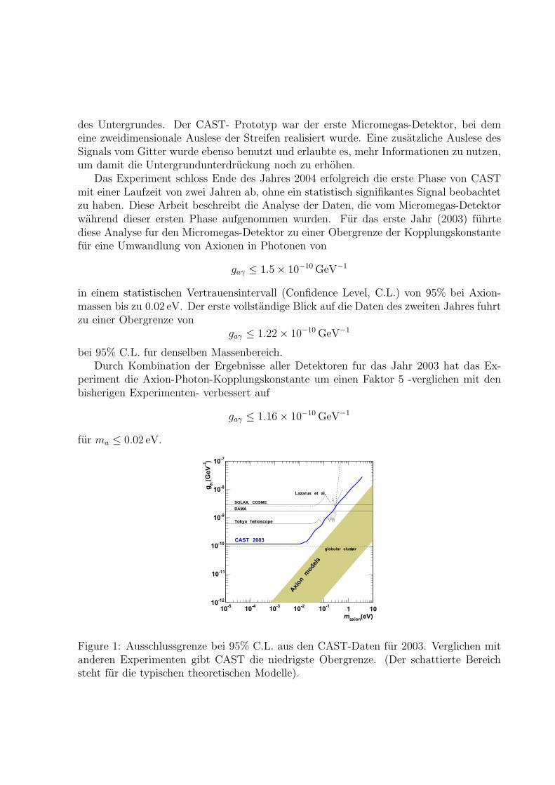
des Untergrundes. Der CAST- Prototyp war der erste Micromegas-Detektor, bei demeine zweidimensionale Auslese der Streifen realisiert wurde. Eine zusatzliche Auslese desSignals vom Gitter wurde ebenso benutzt und erlaubte es, mehr Informationen zu nutzen,um damit die Untergrundunterdruckung noch zu erhohen.
Das Experiment schloss Ende des Jahres 2004 erfolgreich die erste Phase von CASTmit einer Laufzeit von zwei Jahren ab, ohne ein statistisch signifikantes Signal beobachtetzu haben. Diese Arbeit beschreibt die Analyse der Daten, die vom Micromegas-Detektorwahrend dieser ersten Phase aufgenommen wurden. Fur das erste Jahr (2003) fuhrtediese Analyse fur den Micromegas-Detektor zu einer Obergrenze der Kopplungskonstantefur eine Umwandlung von Axionen in Photonen von
gaγ ≤ 1.5 × 10⁻¹⁰ GeV−1
in einem statistischen Vertrauensintervall (Confidence Level, C.L.) von 95% bei Axion-massen bis zu 0.02 eV. Der erste vollstandige Blick auf die Daten des zweiten Jahres fuhrtzu einer Obergrenze von
gaγ ≤ 1.22 × 10⁻¹⁰ GeV−1
bei 95% C.L. fur denselben Massenbereich.Durch Kombination der Ergebnisse aller Detektoren fur das Jahr 2003 hat das Ex-
periment die Axion-Photon-Kopplungskonstante um einen Faktor 5 -verglichen mit denbisherigen Experimenten- verbessert auf
gaγ ≤ 1.16 × 10⁻¹⁰ GeV−1
fur ma ≤ 0.02 eV.
(eV)axion
m
-510
-410
-310
-210
-110 1 10
)- 1
(Ge
Vγ
ag
-1210
-1110
-1010
-910
-810
-710
Axi
on m
odel
s
DAMA
SOLAX, COSME
Tokyo helioscope
Lazarus et al.
globular clusters
CAST 2003
Figure 1: Ausschlussgrenze bei 95% C.L. aus den CAST-Daten fur 2003. Verglichen mitanderen Experimenten gibt CAST die niedrigste Obergrenze. (Der schattierte Bereichsteht fur die typischen theoretischen Modelle).
Abstract
The CAST Experiment completed its first phase in the end of 2004, after having runsuccessfully for two years. The results of the data analysis of the Micromegas detectorat CAST for 2003 and a first result of 2004 are presented here. This experiment has asensitivity of almost a factor 100 better compared with previous searches.
The coupling constant of axions of mass up to 0.02 eV to photons has been restrictedwith a 95% Confidence Level to
gaγ ≤ 1.50 × 10⁻¹⁰ GeV−1
for the 2003 Micromegas detector [and gaγ ≤ 1.16 × 10⁻¹⁰ GeV−1 after combining theresult of all the detectors of the experiment]. The preliminary limit acquired for the 2004data is more strict, at
gaγ ≤ 1.21 × 10⁻¹⁰ GeV−1
concerning the Micromegas detector.

Contents
1 Introduction 1
2 Axions 32.1 The strong-CP Problem and its solution . . . . . . . . . . . . . . . . . . . 32.2 Introducing the axion . . . . . . . . . . . . . . . . . . . . . . . . . . . . . . 52.3 Axion Properties . . . . . . . . . . . . . . . . . . . . . . . . . . . . . . . . 6
2.3.1 Coupling to Gluons . . . . . . . . . . . . . . . . . . . . . . . . . . . 62.4 Axion Models . . . . . . . . . . . . . . . . . . . . . . . . . . . . . . . . . . 10
2.4.1 The visible axions . . . . . . . . . . . . . . . . . . . . . . . . . . . . 102.4.2 The invisible axions . . . . . . . . . . . . . . . . . . . . . . . . . . . 10
2.5 Limits on axion properties from Cosmology and Astrophysics . . . . . . . . 122.6 Axion Detection . . . . . . . . . . . . . . . . . . . . . . . . . . . . . . . . . 16
3 The CERN Axion Solar Telescope Experiment 193.1 The Sun as a source of Axions . . . . . . . . . . . . . . . . . . . . . . . . . 19
3.1.1 Solar axion detection in a magnetic field . . . . . . . . . . . . . . . 223.2 The Experiment . . . . . . . . . . . . . . . . . . . . . . . . . . . . . . . . . 243.3 The detectors . . . . . . . . . . . . . . . . . . . . . . . . . . . . . . . . . . 30
3.3.1 The X-ray focusing device . . . . . . . . . . . . . . . . . . . . . . . 303.3.2 The Time Projection Chamber . . . . . . . . . . . . . . . . . . . . 323.3.3 MICROMEGAS . . . . . . . . . . . . . . . . . . . . . . . . . . . . . 34
3.4 Collateral . . . . . . . . . . . . . . . . . . . . . . . . . . . . . . . . . . . . 35
4 The MICROMEGAS detector 374.1 Phenomenology of particle detection in a gas . . . . . . . . . . . . . . . . . 37
4.1.1 Photons . . . . . . . . . . . . . . . . . . . . . . . . . . . . . . . . . 374.1.2 Electrons . . . . . . . . . . . . . . . . . . . . . . . . . . . . . . . . 384.1.3 Excitation and Ionization in Gases . . . . . . . . . . . . . . . . . . 424.1.4 Transport of ions and electrons in gases . . . . . . . . . . . . . . . . 434.1.5 Multiplication . . . . . . . . . . . . . . . . . . . . . . . . . . . . . . 46
4.2 Gaseous Detectors; A brief walk through history . . . . . . . . . . . . . . . 474.3 MICROMEGAS . . . . . . . . . . . . . . . . . . . . . . . . . . . . . . . . . 51
4.3.1 Description of the CAST Prototype . . . . . . . . . . . . . . . . . . 55
vii

viii
4.3.2 The Set Up . . . . . . . . . . . . . . . . . . . . . . . . . . . . . . . 574.3.3 Readout electronics and the Data Acquisition (DAQ) . . . . . . . . 58
5 The Search for Axions with MICROMEGAS 655.1 The 2003 Data taking . . . . . . . . . . . . . . . . . . . . . . . . . . . . . 655.2 The Analysis of the 2003 data . . . . . . . . . . . . . . . . . . . . . . . . . 67
5.2.1 Strips . . . . . . . . . . . . . . . . . . . . . . . . . . . . . . . . . . 695.2.2 The signal from the mesh . . . . . . . . . . . . . . . . . . . . . . . 715.2.3 Calibration . . . . . . . . . . . . . . . . . . . . . . . . . . . . . . . 725.2.4 Building the X-ray profile . . . . . . . . . . . . . . . . . . . . . . . 735.2.5 Spectra . . . . . . . . . . . . . . . . . . . . . . . . . . . . . . . . . 83
5.3 The Results of the 2003 analysis . . . . . . . . . . . . . . . . . . . . . . . . 88
6 The 2004 Data 936.1 The 2004 Data Taking . . . . . . . . . . . . . . . . . . . . . . . . . . . . . 936.2 The Analysis of the 2004 data . . . . . . . . . . . . . . . . . . . . . . . . . 95
6.2.1 Conditions and Efficiency . . . . . . . . . . . . . . . . . . . . . . . 956.2.2 Spectra . . . . . . . . . . . . . . . . . . . . . . . . . . . . . . . . . 100
6.3 Study of the Systematics . . . . . . . . . . . . . . . . . . . . . . . . . . . . 1006.3.1 Results . . . . . . . . . . . . . . . . . . . . . . . . . . . . . . . . . . 112
7 Conclusions and Outlook 115
Chapter 1
Introduction
The discussion on axions has its roots in the strong-CP problem: theory predicts a CPviolation from the strong interactions, which Nature has never exhibited in any experi-ment. Peccei and Quinn introduced a new symmetry to solve the problem, a symmetrywhich hid a new, almost massless boson, the axion. The axion is rather fascinating if oneis to judge by the number and variety of applications its existence has suggested:
• rather aged as one of the two survivor candidates of the “Dark Matter” that shouldbe around us, accounting for the 25% of the density of the Universe, or even
• a baby having just been born in the core of a star, like the Sun.
Cosmology and astrophysics have already given the first constraints on the propertiesof the axions (regarding their mass and couplings to fermions, nucleons and photons).Gathering all these bounds, only a small window in the mass range of µeV to some tensof meV “survives” to allow for axions to sit in. Several experiments have been looking foraxions taking advantage of the Primakoff effect. According to this process, an axion canbe born from a photon in the presence of an electric or magnetic field, and vice versa, theaxion has a chance to convert to a photon under similar conditions.
Several techniques have been invented and put into act for the detection of axions.Tunable microwave cavities permeated with magnetic field are waiting for relic axionslingering in our galactic halo to be converted into photons; laser beams are sent throughmagnetic fields or on walls, in the hope of producing axions; conversion of axions incrystals has been exploited through a Primakoff-Bragg effect; magnets are pointing atthe Sun, offering the axion tempting reasons to leave the signature of its existence via aphoton.
The CAST experiment is one of these helioscopes. It uses a nearly 10 m long LargeHadron Collider (LHC) decommissioned magnet that can reach a magnetic field of 9 T,which sits on a movable platform. The movement of the platform allows the magnet tobe aligned with the Sun for approximately 100 min during sunset and just as much duringsunrise. Any excess over the background which appears only during tracking times, willbe a signal of axions-converted-to-photons.
1
2 CHAPTER 1. INTRODUCTION
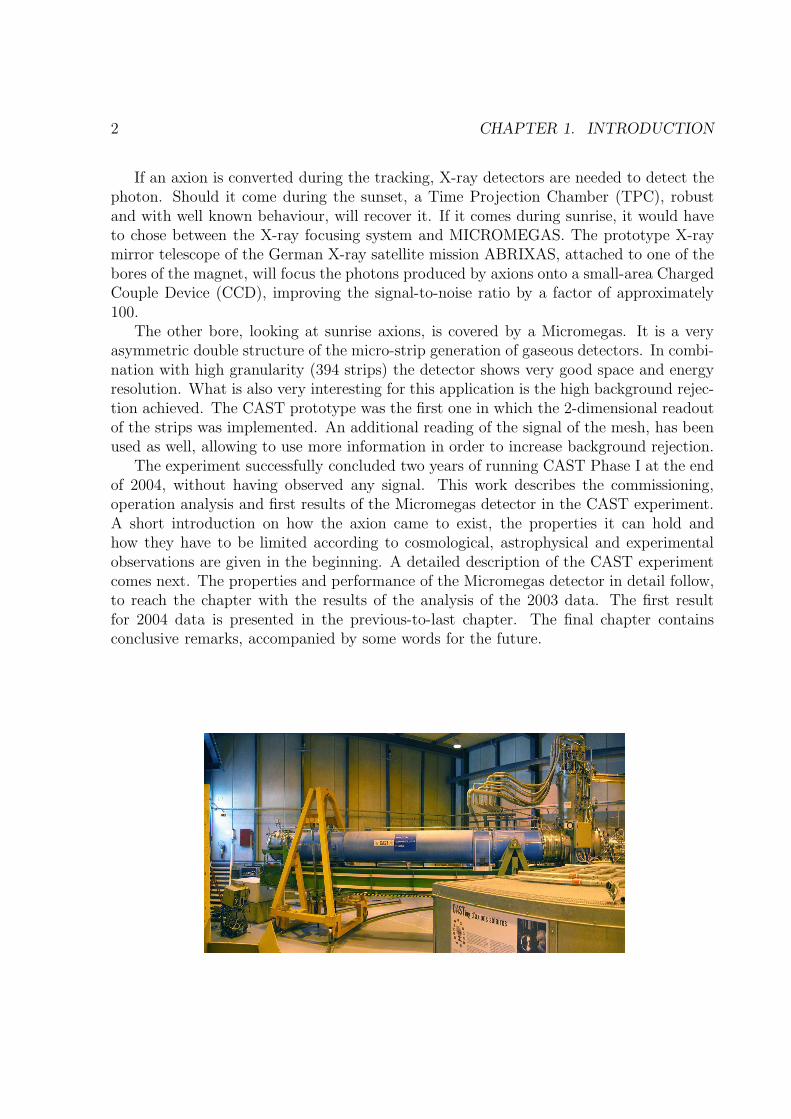
If an axion is converted during the tracking, X-ray detectors are needed to detect thephoton. Should it come during the sunset, a Time Projection Chamber (TPC), robustand with well known behaviour, will recover it. If it comes during sunrise, it would haveto chose between the X-ray focusing system and MICROMEGAS. The prototype X-raymirror telescope of the German X-ray satellite mission ABRIXAS, attached to one of thebores of the magnet, will focus the photons produced by axions onto a small-area ChargedCouple Device (CCD), improving the signal-to-noise ratio by a factor of approximately100.
The other bore, looking at sunrise axions, is covered by a Micromegas. It is a veryasymmetric double structure of the micro-strip generation of gaseous detectors. In combi-nation with high granularity (394 strips) the detector shows very good space and energyresolution. What is also very interesting for this application is the high background rejec-tion achieved. The CAST prototype was the first one in which the 2-dimensional readoutof the strips was implemented. An additional reading of the signal of the mesh, has beenused as well, allowing to use more information in order to increase background rejection.
The experiment successfully concluded two years of running CAST Phase I at the endof 2004, without having observed any signal. This work describes the commissioning,operation analysis and first results of the Micromegas detector in the CAST experiment.A short introduction on how the axion came to exist, the properties it can hold andhow they have to be limited according to cosmological, astrophysical and experimentalobservations are given in the beginning. A detailed description of the CAST experimentcomes next. The properties and performance of the Micromegas detector in detail follow,to reach the chapter with the results of the analysis of the 2003 data. The first resultfor 2004 data is presented in the previous-to-last chapter. The final chapter containsconclusive remarks, accompanied by some words for the future.
Chapter 2
Axions
A brief introduction on how the axion came to be sought after by many ex-periments, is given in this chapter: what the axion is, its properties and thelimits set on them by astrophysics, cosmology and experiments so far.
2.1 The strong-CP Problem and its solution
A problem
A spontaneously broken symmetry is a symmetry that is valid for the Lagrangian butnot for the vacuum (ground) state of the system. As a general theorem, whenever acontinuous global symmetry is spontaneously broken, the spectrum will have a massless,spin-zero boson (Nambu-Goldstone boson). If the symmetry is not exact though, theassociated particle has a small mass, and is called a “pseudo-Goldstone boson”.
When examining the Quantum Chromodynamics (QCD) Lagrangian, given (for fflavour of quarks) by
LQCD = −∑
f
q(γµ 1
iDµ +mf
)qf − 1
4Gµν
a Gaµν , (2.1)
there is a global symmetry in the limit for mf → 0, denoted as G = U(f)R × U(f)L.Regarding the u and d quarks – the masses are relatively small and in the limit they areset to zero – the theory shows a symmetry U(2)L × U(2)R. The vectorial part of thissymmetry U(2)L+R (and its subgroup U(1)V = U(1)L+R) is an exact symmetry. On the
3
4 CHAPTER 2. AXIONS
other hand, the axial part (U(2)A = U(2)L−R) is not preserved by the QCD vacuum, and–following the above mentioned theorem– four Goldstone bosons are expected. Threeof them (corresponding to the SU(2)A breaking) have been noticed; the pion tripletπ− , π0 , π+. However the expected fourth boson, related to the U(1)A breaking, does notexist. This is the U(1)A problem1,2.
It turns out [3, 4], that the answer to the problem lies between the fact that U(1)A
has a chiral (otherwise called axial or triangle or Adler-Bell-Jackiw) anomaly and thatthe ground state (vacuum) of QCD is non-trivial. In fact, the QCD vacuum has infinitelydegenerate vacua, topologically different. The transition from one vacuum class to anotheris classically forbidden, yet due to quantum tunneling, this transition has a non-zeroamplitude. Instantons describe a solution, localized in space and time, in which a vacuumof class n− 1 evolves into another vacuum, of class n. This integer, n, is the topologicalwinding number, labeling each of the vacua. The superposition of the various vacua iscalled the Θ-vacuum, and can be written as a function of the parameter Θ :
|Θ >=∑
n
e−inΘ |n > . (2.2)
At the same time, considering the effect of the chiral anomaly of the U(1)A symmetry,an extra term is added to the Lagrangian, changing it to
LeffQCD = LQCD + Θ
g2
32πGµν
a Gaµν , (2.3)
(where Θ is the above mentioned Θ parameter) or, including the electroweak interactionsto
LeffSM = LSM + Θ
g2
32πGµν
a Gaµν . (2.4)
where LSM is the Standard Model Lagrangian. Here Θ is substituted by an effective Θparameter
Θ = Θ + Arg(detM) , (2.5)
which takes into account both QCD and electroweak information: quarks acquire theireffective masses through the breakdown of the electroweak symmetry, and M is the quarkmass matrix.
Because of the non-trivial properties of the Θ-vacuum, and the axial anomaly of U(1)A
it was shown [3, 4] that U(1)A is not really a quantum symmetry of QCD, and thereforeno Nambu-Goldstone boson is expected associated with this symmetry; η does not needto be lighter than it is.
1Put in a different way, the only other possible particle, the η meson, although it has the right quantumnumbers (JP = 0−) is remarkably heavy (mη = 958 MeV while mπ = 135 MeV ). So another expressionof the U(1)A problem would be “why is η so heavy?”.
2For a complete discussion on the subject, one should refer to [1, 2].
2.2. INTRODUCING THE AXION 5
Another problem
As much as it helped resolve the U(1)A problem, the implementation of Θ induces anotherone: its presence implies violation of the CP invariance in QCD, which has never beenobserved.
Electric dipole moments are the most interesting parameters connected to CP vio-lation. The electric dipole moment of the neutron has a strong experimental bound at|dn| ≤ 12 × 10−26 e cm. However, a simple dimensional analysis of this quantity yieldsa value for dn ∼ 10−16 Θ e cm. This automatically constrains Θ to Θ <∼ 10−9 . Thesmallness of Θ implies an extreme fine-tunning of Θ to the value of Arg detM , for thesecontributions to cancel to the order of Θ. The question of the smallness of Θ, is knownas “the Strong-CP problem”.
A solution to the strong-CP problem
An elegant answer to this problem was supplied by Peccei and Quinn [5, 6]: the extensionof the Standard Model with an additional, spontaneously broken, global chiral U(1) sym-metry (the U(1)PQ), such that changes to Θ are equivalent to changes in the definitionsof the various fields of Leff
SM. In that case, any change in Θ has no physical consequenceand is equivalent to a Θ = 0, leaving no strong-CP violation. From the breaking of thesymmetry a pseudo Nambu-Goldstone boson emerges, the axion3 [7, 8].
2.2 Introducing the axion
If fa is the scale of the spontaneous breakdown of U(1)PQ, the axion field a(x) willtransform under the new symmetry as
a(x)PQ→ a(x) + αfa . (2.6)
Because of the chiral anomaly of this symmetry, the axion will couple to gluons, resultingin the appearance of an extra term (linearly depending on a(x)) in the Lagrangian
Laxion =a(x)
faξg2
32π2Gµν
a Gaµν −1
2∂µa∂
µa + L(∂µa, ψ) (2.7)
for ξ a model depending parameter, 12∂µa∂
µa the kinetic energy of the axion field andL(∂µa, ψ) stands for the possible interaction of the axion field with a fermion ψ. The firstterm of this equation gives the axion field an effective potential, allowing it to relax notin all values of vacuum, but only in those that minimize this potential
⟨∂Veff
∂a
⟩= 0 =⇒< a >= −fa
ξΘ . (2.8)
3The axion was named after a laundry detergent,“since they clean up a problem with an axial current”[9].
6 CHAPTER 2. AXIONS
The strong-CP problem is solved: the physical axion field
aphys = a − < a > (2.9)
absorbs the Θ dependent term and no violation occurs.All is left to do is experimentally verify that the axion exists.
2.3 Axion Properties
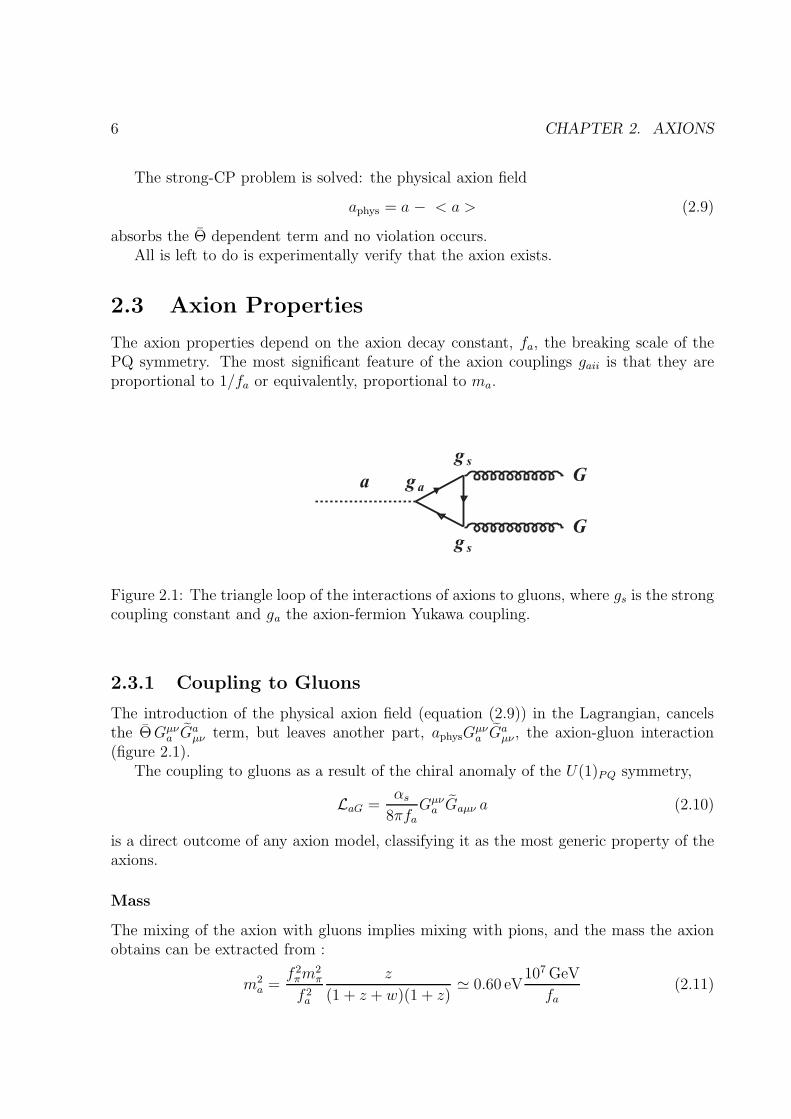
The axion properties depend on the axion decay constant, fa, the breaking scale of thePQ symmetry. The most significant feature of the axion couplings gaii is that they areproportional to 1/fa or equivalently, proportional to ma.
a ag
sg
sg
G
G
Figure 2.1: The triangle loop of the interactions of axions to gluons, where gs is the strongcoupling constant and ga the axion-fermion Yukawa coupling.
2.3.1 Coupling to Gluons
The introduction of the physical axion field (equation (2.9)) in the Lagrangian, cancelsthe ΘGµν
a Gaµν term, but leaves another part, aphysG
µνa Ga
µν , the axion-gluon interaction(figure 2.1).
The coupling to gluons as a result of the chiral anomaly of the U(1)PQ symmetry,
LaG =αs
8πfaGµν
a Gaµν a (2.10)
is a direct outcome of any axion model, classifying it as the most generic property of theaxions.
Mass
The mixing of the axion with gluons implies mixing with pions, and the mass the axionobtains can be extracted from :
m2a =
f 2πm
2π
f 2a
z
(1 + z + w)(1 + z)≃ 0.60 eV
107 GeV
fa(2.11)
2.3. AXION PROPERTIES 7
where fπ ≃ 93 MeV and mπ = 135 MeV are the decay constant and mass of the pion,respectively, and
z ≡ mu/md ≃ 0.55 ± 0.1 (2.12)
w ≡ mu/ms = 0.029 ± 0.003
the quark mass ratios [10]. z is a quantity largely discussed. The value itself and itsuncertainty vary significantly among calculations, for example from [11] one acquiresz ≃ 0.553 ± 0.043 while the Particle Data Group [12] gives a value of 0.3 <∼ z <∼ 0.7.
Coupling to photons
The coupling of the axions to photons arises as a result of two contributions:
• Inevitably, the electromagnetic anomaly (the mixing with the neutral pions) gener-ates coupling of the axions to photons as well as nucleons.
• In analogy to the coupling to gluons, if the fermions carrying PQ charges carryelectric charges as well, they will couple (through a Yukawa coupling) the axion totwo photons, via a triangle loop.
The two parts are shown schematically in figure 2.2.The interaction will be according to
Laγ = −gaγ
4F µν
a Faµν = gaγ~E ~B a (2.13)
where
gaγ =α
2πfa
(E
N− 2(4 + z + w)
3(1 + z + w)
). (2.14)
for F µνa the electromagnetic field strength tensor, Faµν its dual, α the fine structure
constant and gaγ the coupling constant. z and w are as defined above, equation (2.11).Introduced in equation (2.14), it becomes
gaγ =α
2πfa
(E
N− 1.93 ± 0.08
). (2.15)
The coupling constant includes a factor E/N , the ratio of the two anomaly coefficients,E the electromagnetic anomaly and N the color anomaly. If Qj are the electric chargesof the PQ fermions and Xj their PQ charge, E,N are defined as follows:
E ≡ 2∑
j
XjQ2jDj N ≡
∑
j
Xj , (2.16)
were Dj = 1 for color singlets (charged leptons) and Dj = 3 for color triplets (quarks).Different models present different couplings to photons, because the values of these num-bers are different for each one.

8 CHAPTER 2. AXIONS
a γ
γ
a π
γ
γ
ii.
i.
0
Figure 2.2: The two contributions to the axion-photon coupling: one from the couplingto fermions that carry PQ charge (i), and the second from the axion-pion mixing (ii).
Coupling to fermions
The coupling of axions with fermions is the main one distinguishing several models. Elec-trons and quarks would show Yukawa couplings to axions, if they (electrons and quarks)carry PQ charge. Because free quarks do not exist, the effective coupling of axions tonucleons can be studied. The tree-level interaction between axions and fermions, in ageneral form can be represented by
Laf =gaf
2mfΨfγ
µγ5Ψf∂µa . (2.17)
f denotes the type of fermion (electron, nucleon) and
gaf =Cf mf
fa(2.18)
the equivalent Yukawa coupling if mf is the fermion mass. Cf stands for the effective PQcharge, a model-dependent quantity.
2.3. AXION PROPERTIES 9
Tree-level coupling to electrons
Depending on the model, electrons may carry PQ charge, and therefore will interact asequation (2.17) describes. Following equation (2.18) in this case,
gtreeae =
Ceme
fa= Ce0.85 × 10−10ma . (2.19)
Here Ce = X ′e/N , for X ′
e the “effective” PQ charge of the electron.
Radiatively induced coupling to electrons
There are models for which the shifted charge X ′e = 0. For reasons of completeness,
one should mention that even in that case, there exists an axion-to-electron couplingeffectively, connected to a loop correction due to the interaction of axions with photons,with the form [13]:
gloopae =
3α2
4π2
me
fa
[E
Nln
(fa
me
)− 2(4 + z + w)
3(1 + z + w)ln(
ΛQCD
me
)]. (2.20)
where ΛQCD is the QCD scale.One can see that this loop correction is much weaker than the tree-level.
Coupling to nucleons
The coupling of axions to nucleons consists of two compounds, one derived from the tree-level coupling of axions to up and down quarks, and another emerging from the axion-pionmixing. Similarly to electrons, the coupling can be described by equation (2.18), giving
gaN =CNmN
fa
(2.21)
for the effective PQ charge of the nucleon CN . Because of the two different parts ofthe interaction, CN is a combination of the quarks’ masses, and reads for protons andneutrons respectively:
Cp = (Cu − η)∆u+ (Cd − ηz)∆d+ (Cs − ηw)∆s
Cn = (Cu − η)∆d+ (Cd − ηz)∆u+ (Cd − ηw)∆s , (2.22)
with the forementioned (equation (2.11)) definitions of z, w and for η ≡ 1/(1 + z + w).∆u is the fraction of the nucleon’s spin carried by the u quark, and the rest respectively.Substituting [14]
∆u = +0.80 ± 0.04 ± 0.04 (2.23)
∆d = −0.46 ± 0.04 ± 0.04
∆s = −0.12 ± 0.04 ± 0.04
(statistical and systematic errors shown) in equation (2.22) and subsequently to equation(2.21), the axion-to-nucleon coupling constant is calculated.

10 CHAPTER 2. AXIONS
2.4 Axion Models
Equation (2.11) exhibits the clear dependence of the axion’s mass on the decay constantfa. Different values of fa classify axions in different categories: the larger the scale, themore weakly coupled and lighter the axion.
2.4.1 The visible axions
A very simple assumption (in fact the one made originally by Peccei and Quinn [5, 6]),would be that the decay constant is of the same order as the electroweak scale, so fa ≃250 GeV. This would be translated to an axion with a mass of about 100 keV. However,several experiments have excluded the existence of such ‘visible’ axions rather soon:axions of that mass would be expected in the process
K+ → π+a .
A strong bound was set by the non observation of this process in KEK [15], for thebranching ratio
BR(K+ → π+ Nothing) ≤ 3.8 × 10⁻⁸ ,
where “Nothing” is interpreted as a long lived axion which escapes detection, the strongestevidence against the visible axions.
2.4.2 The invisible axions
At the other end, if the scale fa is much larger than fweak, the coupling of the axionbecomes weaker so much that it can have eluded all preliminary searches; it would be‘invisible’. These models introduce a complex scalar field φ with a very large vacuumexpectation value < φ >= fPQ/
√2 ≫ fweak. This field does not participate in the elec-
troweak interactions. Two groups of models for the invisible axions have been considered:the KSVZ and DFSZ. Both groups are successful in their goal, to solve the strong-CPproblem, however they conclude in different couplings of the axion.
The KSVZ axion
The Kim-Shifman-Vainshtein-Zakharov model [16] for axions suggests the existence ofnew, heavy quarks that carry Peccei-Quinn charge, while the usual leptons and quarks donot. The last statement puts Ce = 0 forbidding the KSVZ axion to couple to electronsin the tree level, and for this reason is known as the “hadronic” axion. Still, there is avery weak coupling to electrons for this type of axions as well, the radiatively inducedone, discussed above.
Although normal quarks in this model do not feel the PQ symmetry (meaning Cu =Cd = Cs = 0), axions do couple with nucleons, according to equation (2.21). The couplingconstants to nucleons are determined for the following values of the PQ-charge parameters(equations (2.22)):

2.4. AXION MODELS 11
Cp = −0.34 (2.24)
Cn = 0.01 ,
leaving room for the Yukawa couplings of axions to protons and neutrons respectively
gap =Cpmp
fa
= −5.32 × 10⁻⁸ma (2.25)
gan =Cnmn
fa= 1.57 × 10⁻⁹ma .
Turning to the coupling to photons, equation (2.15) shows the dependence on the ratioE/N . Different models, within the KSVZ frame, give different values for this ratio. Therecan be models with E/N ≃ 2 [17], that suppress the photon coupling. In that case, thedominant contribution is from the coupling of axions to nucleons.
The DFSZ axion
In contrast to the previous model, in the Dine-Fischler-Srednicki-Zhitnitskii model [18]normal quarks and leptons do feel the PQ symmetry (carry PQ charge). The ordinaryHiggs field is substituted by two new ones, having vacuum expectation values f1, f2 re-spectively. In any Grand Unified Theory (GUT) for a given family of quarks and fermions,the ratio E/N equals to 8/3, making
gDFSZaγ = 0.75
α
2πfa. (2.26)
for the coupling to photons.Since this ratio is given, the free parameters in this type of axions are two: the scale
fDFSZa , and the ratio x = f1/f2. In fact, the PQ-charge of the quarks and leptons are
functions4 of x (or rather β, defined as cos2 β = x2(x2 + 1)) and hence the couplingconstants to fermions are as well. The effective PQ charges for the fermions for thismodel, for Nf number of families, are as follows:
Ce = Cs = Cd =cos2 β
Nf
(2.27)
Cu + Cd =1
Nf
Cu − Cd = −cos2 β
Nf,
4Following the notation in [14]
12 CHAPTER 2. AXIONS
leading to
Ce = Cs = Cd =cos2 β
Nf(2.28)
Cu =sin2 β
Nf
.
Accepting that Nf = 3, equations (2.22) conclude to
Cp = −0.08 − 0.46 cos2 β (2.29)
Cn = −0.14 + 0.38 cos2 β .
2.5 Limits on axion properties from Cosmology and
Astrophysics
Cosmological constraints
In order to derive information on the axion coupling and mass, one can deduct what theevolution of the axion expectation value would be through the Universe’s life5. In theearly Universe, this value is zero (Θ = 0 conventionally), but as soon as the Universecools down to a temperature of the same range as the Peccei-Quinn scale, the expectationvalue of the axion field takes some chance value Θi (initial “misalignment”). Cooling downto a temperature where the axion mass becomes comparable to the Universe expansionrate, the axion field starts to settle down and oscillate around its final dynamical value(Θ = 0). The energy density accumulated in this oscillations of the axion field, shouldnot exceed the energy density which closes the Universe. Expressing the abundance ofaxions Ωah
2 as a function of the misalignment angle
Ωah2 ≃ 1.9 × 3±1
(1µ eV
ma
)1.175
Θ2i f(Θi) (2.30)
where h2 is the Hubble constant (in units of 100 kms−1Mpc−1), and any anharmonic cor-rections on the axion potential are incorporated in f(Θi). The Wilkinson MicrowaveAnisotropy Probe (WMAP) data gives a matter density of Ωmh
2 = 0.135+0.008−0.008 [23]. As-
suming an abundance for the axions of the same order, and they would dominate theCold Dark Matter of the Universe, if ma was of the order of µeV. The breakdown of acontinuous U(1) symmetry generally allows a one-dimensional topological solution with alinear mass density, determined by the parameter u2 of the symmetry breaking. In thatcase, strings form in the cosmic evolution.
5A further discussion on the cosmological and astrophysical constraints can be found in the reportsand reviews of Kim [19], Turner [20] and Raffelt [21], as well as in the PDG [12].
2.5. LIMITS ON AXION PROPERTIES FROM COSMOLOGY AND ASTROPHYSICS13
The axion models have spontaneously broken U(1)PQ symmetries, therefore in the casethat inflation did not occur at all or if it did, it occurred after the spontaneous breakingof this symmetry, cosmic axion strings would appear. The axion production through thismechanism depends on the average energy of an axion produced by string dissipation attime t. There is a controversy over the matter between Battye and Shellard [24] andSikivie et al. [25, 26]: according to Battye and Shellard, following the notion that theenergy of the axionic strings turns into axions, the mass density that thus produced axionswould contribute would be
Ωstringh2 ≃ maeV
10−3
−1.175
, (2.31)
restricting the axion mass toma >∼ 10−4 eV .
On the other hand, Sikivie et al.’s reasoning, that the string radiation goes more intokinetic axion energy, these axions wouldn’t increase the density of relic axions significantlymore than the “misalignment mechanism” given by equation (2.30). If they are correct,the axion mass should be
ma >∼ 10−6 eV .
Finally, it has been noted that axions with a mass above 0.1 eV, called “multi-eV”axions [40], have lifetimes which are long enough to support that not all relic axions havedecayed until now, yet short enough for quite some of them to be decaying at present.The produced photons must be monoenergetic and will provide line radiation that couldbe detected.
This discussion covers the case where axions were never in thermal equilibrium, mean-ing that the scale fa is quite large (fa ≥ 108 GeV) and axions are weakly interacting. Inthe case that they interacted strongly and the scale were small enough (fa ≤ 108 GeV),axions would have been in good thermal contact with the universal plasma and thereshould exist a background sea of invisible axions. Astrophysical arguments disfavour thispossibility.
Constraints introduced by Astrophysics
The existence of the axion, assumed to be produced in the stellar plasma, would meana novel energy-loss mechanism for stars. A possible axion emission would modify stellarevolution in a way that it would directly affect an observable, like the lifetime of the star;if axions carry away energy from the star, the star will increase its burning fuel in thecenter, in order to compensate the loss, speeding up its evolution and therefore shorteningits lifetime.
Globular cluster stars have nearly the same age, but differ mainly in their mass. Redgiants and Horizontal Branch (HB) stars provide restrictive bounds on the couplings ofaxions to electrons (DFSZ axions) and photons. Arguments as the one mentioned for thestars’ lifetimes bind the axion-to-photon coupling with
gaγ <∼ 1 × 10⁻¹⁰ GeV−1 , (2.32)
14 CHAPTER 2. AXIONS
and their mass
ma <∼ 0.3(E
N− 1.93 ± 0.08
). (2.33)
A bremsstrahlung process
e− + (A,Z) → e− + (A,Z) + a
would delay the helium flash in the red-giants’ core, allowing the core to accumulate moremass until helium ignition. Observations restrict (for the DFSZ axions)
gDFSZae <∼ 2.5 × 10⁻¹³ GeV−1 . (2.34)
The most restrictive limits come from observations of the newly born SN 1987A, whenreferring to axions produced via nucleon-nucleon-axion bremsstrahlung
N +N → N +N + a
in its core. In that case, the energy-loss of the supernova would result in (i) shorteningthe length of the observed neutrino burst, (ii) a possible increase in the number of countsin the neutrino detectors or (iii) axions would radiatively decay.
Taking into account the observations of Kamiokande II and the Irvine-Michigan-Brookhaven (IBM) detectors, the coupling of axions to nucleons in the range [14]
3 × 10⁻¹⁰ GeV−1 <∼ gaN <∼ 3 × 10⁻⁷ GeV−1 , (2.35)
is excluded, deriving an exclusion range for the mass:
0.01 eV <∼ mKSVZa <∼ 10 eV (2.36)
Heavy hadronic axions could induce nuclear excitations that could deexcite via de-tectable γ-rays. This would mean an increase in the number of observed events in thewater- Cerenkov detectors, hence another mass range [27]
20 eV <∼ mKSVZa
<∼ 20 keV (2.37)
is excluded.
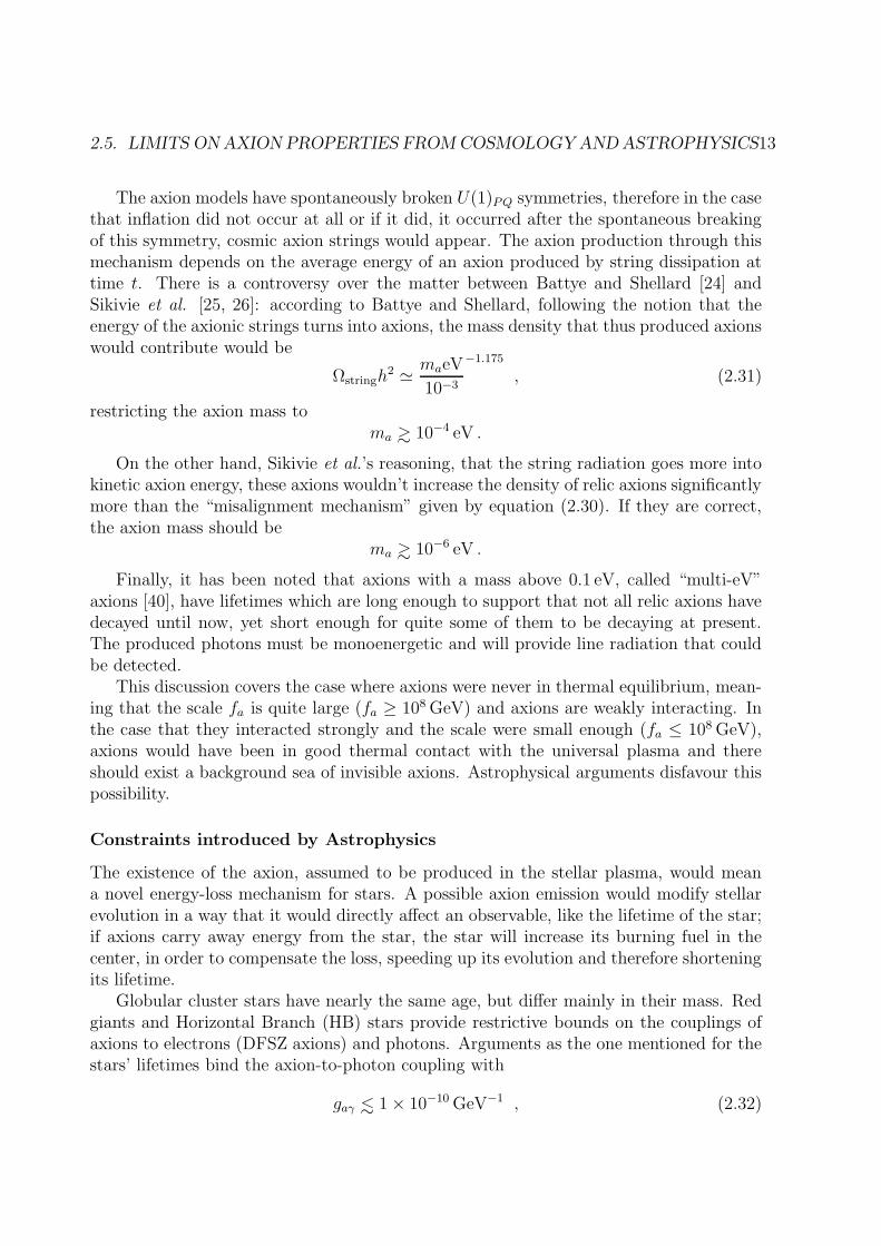
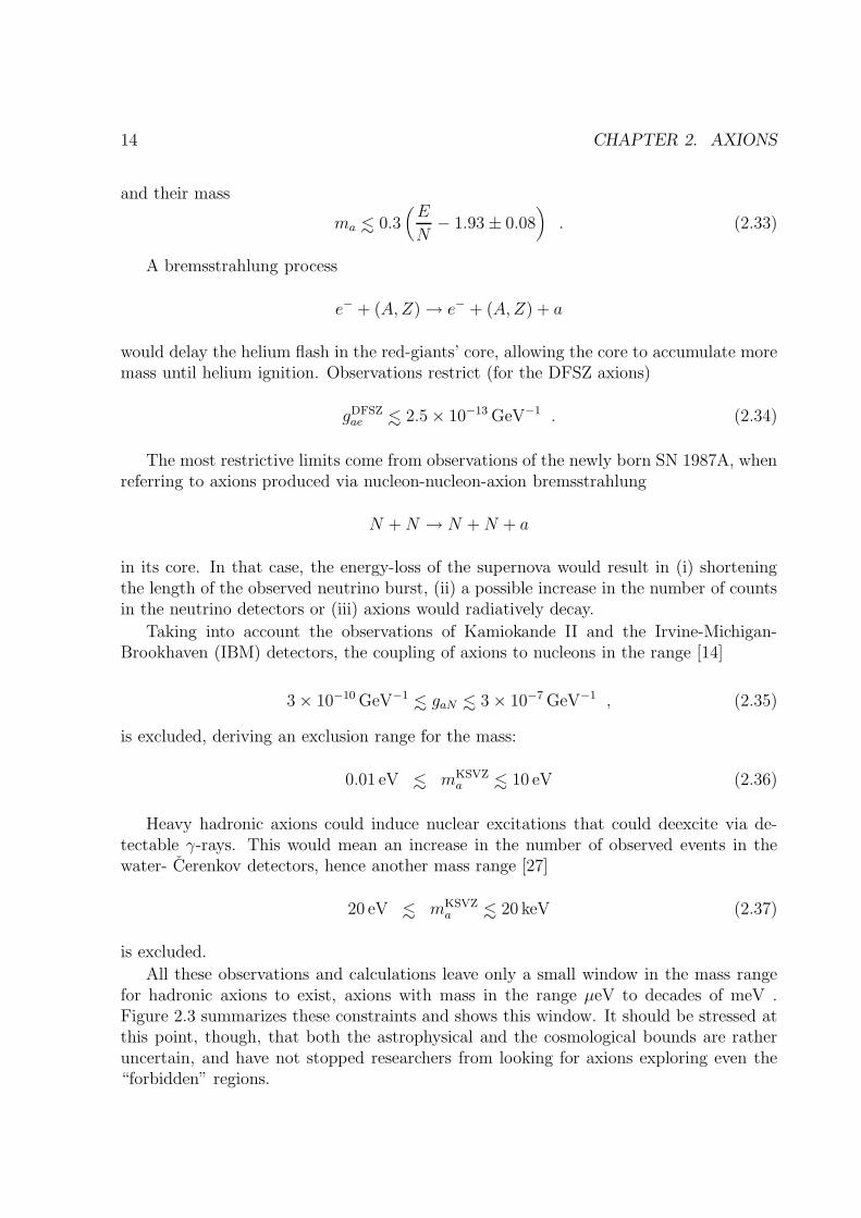
All these observations and calculations leave only a small window in the mass rangefor hadronic axions to exist, axions with mass in the range µeV to decades of meV .Figure 2.3 summarizes these constraints and shows this window. It should be stressed atthis point, though, that both the astrophysical and the cosmological bounds are ratheruncertain, and have not stopped researchers from looking for axions exploring even the“forbidden” regions.
2.5. LIMITS ON AXION PROPERTIES FROM COSMOLOGY AND ASTROPHYSICS15
1010101010 3691215fa
[GeV]
neV µeV meV eV keV ma
Dark
Matter
Inflation
Scenario
String
Scenario
Telescope
SN 1987A:
Too much
energy loss
Too many
events in
detectors
CARRACK
(Kyoto search)
Too much
dark matter
US Axion Search
(Livermore)
Figure 2.3: A summary on the astrophysical and cosmological regions of exclusion forthe axion mass (or, equivalently for the Peccei-Quinn scale fa). The bars with open endsrepresent a rough estimate, for example the one for the globular cluster stars, given herefor the DFSZ model. The SN 1987A limit is for the KSVZ one, but covers approximatelythe DFSZ model as well. The regions with the dots (labeled ‘inflation scenario’ and ‘darkmatter’) are the regions where the axion could be the dark matter and the black ones thesensitivity of the search experiments for galactic dark-matter axions.(Taken from [14])

16 CHAPTER 2. AXIONS
2.6 Axion Detection
Sikivie in 1983 [28], was the first to show that the invisible axions were not really such,proposing several experiments, all based in the axion-to-photon conversion, the Primakoffeffect. Since then, several experimental techniques have been invented for axion searches,and many experiments have come up with results constraining gaγ:
• Microwave cavity experiments: Looking for galactic halo axions, electromag-netic cavities with strong static magnetic field can be helpful (details can be foundin a recent review [29] and the references therein). Fine-tuning the frequency ofthe cavity so that it matches their mass ma, the axions will convert resonantly tophotons, according to the coupling constant (equation (2.14)). Early experiments(Rochester-Brookhaven-Fermilab [30, 31], the University of Florida Experiment [32])were able to scan quite a range of frequencies, and precluded a range in the massaxis of
4.5µeV < ma < 16.3µeV .
Second generation experiments, use –or are going to use– essentially the same tech-niques, but with better sensitivity; the ADMX experiment [33, 34] is continuouslytaking data and have already excluded the mass range
1.9µeV < ma < 3.3µeV .
The experiment will enhance its sensitivity, hopefully toward a definitive axionsearch, implementing a technology based on Superconducting Quantum InterferenceDevices (dc SQUID) [35]. A large-scale detector for axion search has been built inJapan; CARRACK2 (Cosmic Axion Research using Rydberg Atoms in a resonantcavity in Kyoto), is being commissioned, using a Rydberg atom single-quantumdetector [36, 37]. This large-scale detector will cover the region of
2µeV <∼ ma <∼ 30µeV .
Already CARRACK I [38] (the prototype) has searched for axions at the 10µeVregion, and the results are being evaluate.
• Optical and RadioTelescope searches: Searches have also been performed forthe thermally produced axions, the “multi-eV” axions mentioned before. Obser-vations of three well studied clusters (Abell 1413, 2218 and 2256) at Kitt PeakNational Observatory [39, 40] have seen no axion decay line, excluding the range
3 eV < ma < 8 eV .
The radio telescope search, was performed under the assumption that axions dom-inate potential walls. Had axions been present in dwarf galaxies, they would decay
2.6. AXION DETECTION 17
into photons that would be detected as narrow lines in radio telescope power spec-tra ([41]). The observations made in Haystack Observatory raise a bound on theaxion-to-photon coupling at
gaγ < 1.2 × 10⁻⁹ GeV
of axions with a mass298µeV <∼ ma <∼ 363µeV .
• “Shining through a wall” experiments: Given the coupling of axions to pho-tons, one can expect axions to be created when a light beam (usually laser) travelsinside a transverse magnetic field. If the exit of the laser beam is blocked (witha “wall”), only the axion beam will pass through the wall, and entering a secondtransverse magnetic field would be re-converted to detectable photons [42]. An ex-periment done using this technique ([43] and [44]), bound the coupling of axionswith mass
ma < 10−3 eV
to photons togaγ < 6.7 × 10⁻⁷ GeV−1 .
• Polarization experiments: The same experiment put limits on the axion massand coupling to photons using the notation that axions would induce small changesin the polarization state of the photon beam that produces them, responsible fortwo observable effects [45]:
Dichroism As the laser beam propagates in the magnetic field, the component ofthe electric field parallel to the magnetic field (
−→E ‖) will be reduced because of
the production of axions, resulting in dichroism, a rotation of the polarizationvector.
Vacuum Birefringence In the second step, as the axion beam passed throughthe second magnetic field, the initially linearly polarized beam will becomeelliptically polarized (axions will mix again with
−→E ‖).
They restricted [46] the axion-to-photon coupling for
ma < 5 × 10⁻⁴ eV
togaγ < 3.6 × 10⁻⁷ GeV−1 .
A more recent experiment, PVLAS [47] started taking data in late 2002. Althoughtheir primary goal is to measure the magnetically induced birefringence and opticalactivity of the vacuum element, they do have the ability to produce and detectaxions (or axion-like particles) within their apparatus.

18 CHAPTER 2. AXIONS
• Solar axion searches: It has already been discussed that axions could provide anextra cooling mechanism for the stars, in the cores of which they must be producedefficiently. The closest and best known star that can be used for observation is theSun. Using again the Primakoff process, two types of “helioscopes” have been built:
* Axions can interact coherently in the electric field in the neighbourhood of theatomic nuclei in crystals, when the Bragg condition is fulfilled [48]. Germaniumcrystal detectors have been implemented for these searches, and two groupshave looked for axions with this technique, SOLAX [49] and COSME [50].The results they reached are rather similar
gaγ < 2.7 × 10⁻⁹ GeV−1 [SOLAX]
andgaγ < 2.8 × 10⁻⁹ GeV−1 [COSME]
for axion masses up to ma <∼ 1 keV. The DAMA experiment is using NaI(Tl)[51] crystals and achieved a limit of
gaγ < 1.7 × 10⁻⁹ GeV−1 [DAMA] .
* The second type of “helioscopes” make use of the conversion of axions to pho-tons in a magnetic field; they provide the axions coming from the Sun with amagnetic field, transverse to their course, which will help them convert into a’to-be-detected’ photon. The first experiment of this type ([52]) explored tworegions in the mass range :
gaγ < 3.6 × 10⁻⁹ GeV−1 for ma < 0.03 eV
andgaγ < 7.7 × 10⁻⁹ GeV−1 for 0.03 eV < ma < 0.11 eV .
A more recent experiment was performed in Tokyo ([53]), having better sensi-tivity has given the following limits:
gaγ < 6 × 10⁻¹⁰ GeV−1 for ma < 0.03 eV
andgaγ < 6.8 − 10.9 × 10⁻¹⁰ GeV−1 for ma < 0.3 eV .
The Cern Solar Axion Telescope (CAST), that will be described in detail in thefollowing, belongs to this type of searches.
Chapter 3
The CERN Axion Solar TelescopeExperiment
In this chapter the principle and the components of the CAST experiment [54]are described: the concept of the experiment is to have a magnetic field alignedwith the center of the Sun for the longest time interval possible; the incomingaxion will interact with the magnetic field -when the coherence condition isfulfilled- and will be converted to a photon, giving it its energy and momen-tum. Therefore the main components needed to perform the experiment are:the Sun, a magnet (pointing to the direction of the Sun) and photon detec-tors. The sensitivity of the experiment increases with the implementation ofan X-ray focusing device.
3.1 The Sun as a source of Axions
Like in the case of any other star, the interior of the Sun can offer the electric fields (ofnuclei and electrons “targets”) in the plasma to photons that will consequently convertto axions. In the case of small momentum transfer this process is better viewed asinteractions with coherent field fluctuations in the plasma [55], while for a large momentumtransfer it can be viewed as the Primakoff process [56, 57] (figure 3.1):
γ + Ze→ Ze+ a .
Recoil effects of these targets can be neglected considering the rather small (few keV)
19
20 CHAPTER 3. THE CERN AXION SOLAR TELESCOPE EXPERIMENT
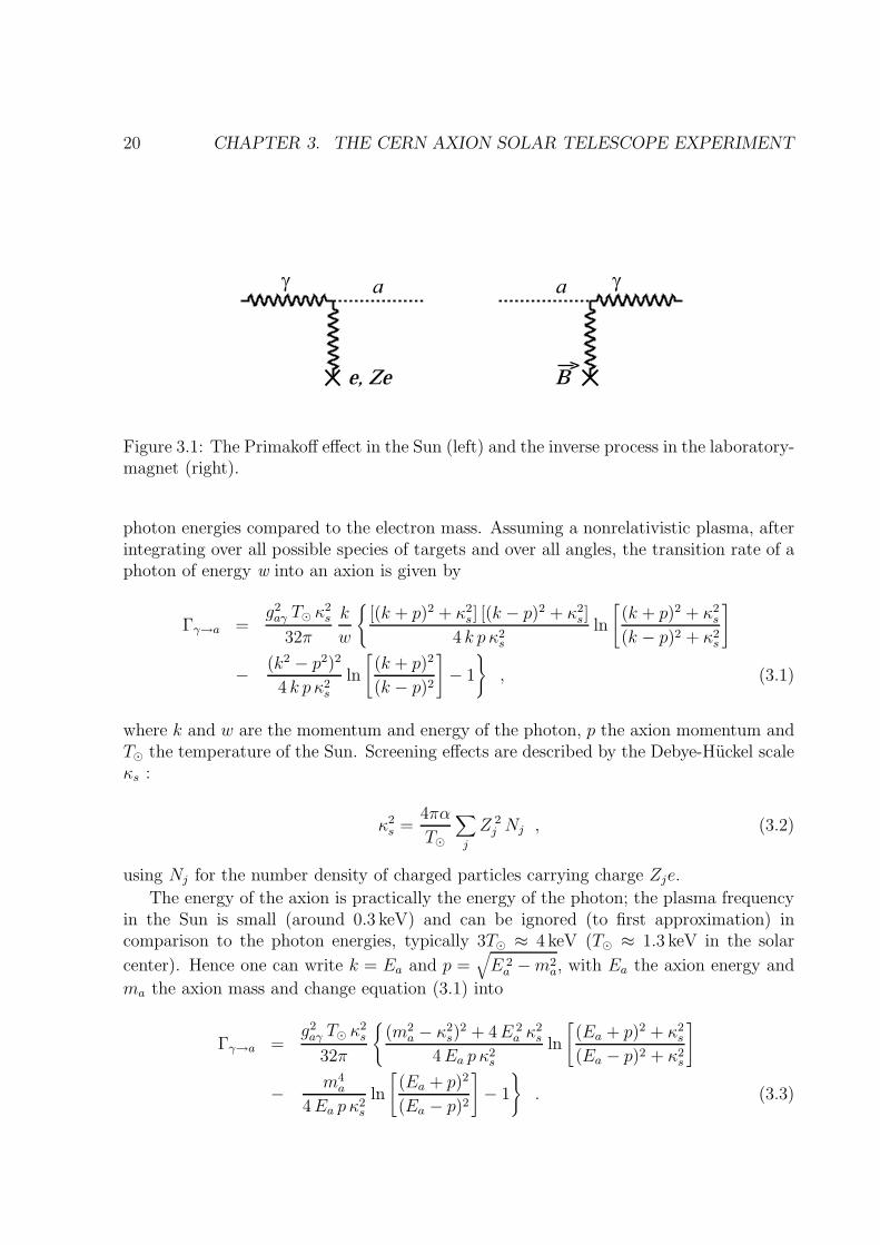
γ a a γ
e, Ze B
Figure 3.1: The Primakoff effect in the Sun (left) and the inverse process in the laboratory-magnet (right).
photon energies compared to the electron mass. Assuming a nonrelativistic plasma, afterintegrating over all possible species of targets and over all angles, the transition rate of aphoton of energy w into an axion is given by
Γγ→a =g2
aγ T⊙ κ2s
32π
k
w
[(k + p)2 + κ2
s] [(k − p)2 + κ2s]
4 k p κ2s
ln
[(k + p)2 + κ2
s
(k − p)2 + κ2s
]
− (k2 − p2)2
4 k p κ2s
ln
[(k + p)2
(k − p)2
]− 1
, (3.1)
where k and w are the momentum and energy of the photon, p the axion momentum andT⊙ the temperature of the Sun. Screening effects are described by the Debye-Huckel scaleκs :
κ2s =
4πα
T⊙
∑
j
Z 2j Nj , (3.2)
using Nj for the number density of charged particles carrying charge Zje.
The energy of the axion is practically the energy of the photon; the plasma frequencyin the Sun is small (around 0.3 keV) and can be ignored (to first approximation) incomparison to the photon energies, typically 3T⊙ ≈ 4 keV (T⊙ ≈ 1.3 keV in the solar
center). Hence one can write k = Ea and p =√E 2
a −m2a, with Ea the axion energy and
ma the axion mass and change equation (3.1) into
Γγ→a =g2
aγ T⊙ κ2s
32π
(m2
a − κ2s)
2 + 4E 2a κ
2s
4Ea p κ2s
ln
[(Ea + p)2 + κ2
s
(Ea − p)2 + κ2s
]
− m4a
4Ea p κ2s
ln
[(Ea + p)2
(Ea − p)2
]− 1
. (3.3)
3.1. THE SUN AS A SOURCE OF AXIONS 21
To obtain the differential flux of axions at Earth, the transition rate is folded over theblackbody photon distribution of the Sun. Integrating over a standard solar model [58]:
dΦa(Ea)
dEa=
1
4 π r2E
∫ R⊙
0d 3r Γγ→a
1
π2
E 2a
eEa/T⊙ − 1(3.4)
where rE is the distance between the Sun and the Earth (rE = 1.50 × 1013 cm) and R⊙
the radius of the Sun.In reference [56], a well approximated analytic formula for the differential axion spec-
trum is given :
dΦa(Ea)
dEa
= 4.02 × 10¹⁰(
gaγ
10−10GeV−1
)2 (Ea/keV)3
eEa/1.08 keV − 1
[cm−2s−1keV−1
]. (3.5)
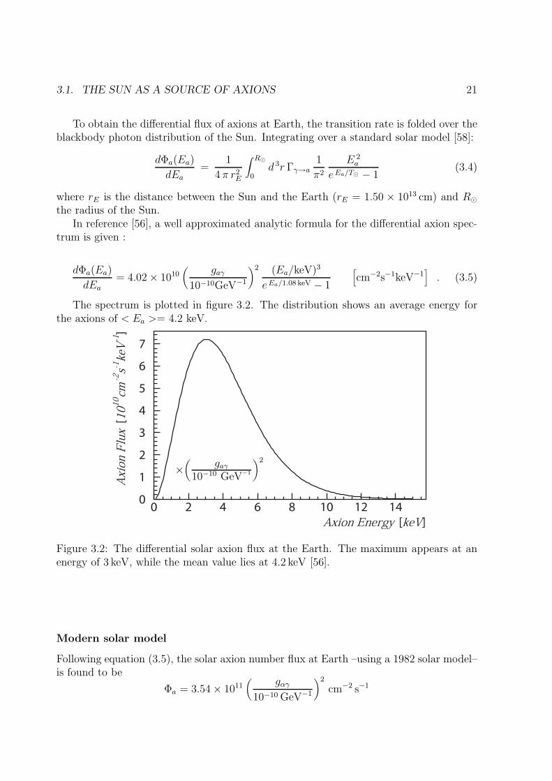
The spectrum is plotted in figure 3.2. The distribution shows an average energy forthe axions of < Ea >= 4.2 keV.
Axion Energy [keV]
Axi
on
Flu
x[1
01
0cm
-2s-1
keV
-1]
0
1
2
3
4
5
6
7
0 2 4 6 8 10 12 14
Figure 3.2: The differential solar axion flux at the Earth. The maximum appears at anenergy of 3 keV, while the mean value lies at 4.2 keV [56].
×(
gaγ
10−10 GeV−1
)2
Modern solar model
Following equation (3.5), the solar axion number flux at Earth –using a 1982 solar model–is found to be
Φa = 3.54 × 10¹¹(
gαγ
10−10 GeV−1
)2
cm−2 s−1
22 CHAPTER 3. THE CERN AXION SOLAR TELESCOPE EXPERIMENT
A more recent calculation [59, 60], using a modern solar model gives
Φa = 3.75 × 10¹¹(
gαγ
10−10 GeV−1
)2
cm−2 s−1
and a fit function for the differential flux :
dΦa(Ea)
dEa= 6.02 × 10¹⁰
(gaγ
10−10GeV−1
)2 (Ea/keV)2.481
eEa/1.205 keV − 1
[cm−2s−1keV−1
]. (3.6)
A comparison between the two equations shows that the axion flux expected dependsonly slightly on the exact solar model.
3.1.1 Solar axion detection in a magnetic field
The Primakoff effect consists practically of an interaction between the axion coming fromthe Sun and a virtual photon provided by the magnetic field. Anyone of those virtualphotons could be the one taking part in this conversion, at any length of the field for whichthe interference will be constructive (the coherence condition). The conversion processremains coherent when the axion and photon fields remain in phase over the length of themagnetic field [61]. Taking this into account, the axion-to-photon conversion probabilityin vacuum is calculated as
Pa→γ =(Bgaγ
2
)2
2L2 1 − cos2(qL)
(qL)2, (3.7)
where B and L are the magnetic field and length. q indicates the momentum transferbetween the axion and the X-ray photon:
q =m2
a
2Ea. (3.8)
The coherence condition then is satisfied for
qL < π . (3.9)
For a 10 m long magnet and the expected energy spectrum (with a mean energy of∼ 5 keV), this condition brings the limit on the mass up to which such an experiment issensitive in vacuum to ma < 0.03 eV.
However, using an X-ray absorbing buffer gas, the transition rate Pa→γ changes ac-cording to equation (3.10), where the absorption in the gas is taken into account.
Pa→γ =(Bgaγ
2
)2 1
q2 + Γ2/4
[1 + e−Γ L − 2e−Γ L/2 cos(qL)
], (3.10)

3.1. THE SUN AS A SOURCE OF AXIONS 23
with Γ the inverse photon absorption length for the X-rays in the medium. In this case,the momentum transfer q becomes
q =
∣∣∣∣∣m2
γ −m2a
2Ea
∣∣∣∣∣ , (3.11)
for mγ the photon effective mass (given by the plasma frequency) in the buffer gas
mγ ≃√
4πne
me= 28.9
√Z
Aρ , (3.12)
where ne is the number density of electrons, me the electron mass, and the dependence onthe atomic number Z and mass A as well as the gas pressure P are evident. In the case of
hydrogen or helium (at 300 K), one can calculate mγ =√P [atm]/15. Now the coherence
is restored for a narrow mass window, for which the “mass” of the photon matches thatof the axion such that
qL < π =⇒√
m2γ −
2πEa
L< ma <
√
m2γ +
2πEa
L, (3.13)
which brings the sensitivity of the mentioned experiment with a helium buffer gas at1 atm1 up to an axion mass of 0.3 eV. Figure 3.3 shows an example of two measurements,one in vacuum and one in 6.08 mbar .
Of most interest is the number of photons Nγ expected after the conversion
Nγ =∫dΦa(Ea)
dEa
S t Pa→γ dEa , (3.14)
where S is the effective area of the detector, and t the measurement time in days. Equation(3.14) exhibits the importance of the measurement’s time, and does not include the factorof the detector’s efficiency.
The agenda of the CAST experiment included the exploitation of every possibility tocover the wider range of potential axion masses, and foresaw two phases:
Phase I covers the conversion of axions-to-photons in vacuum. For the parameters ofCAST (see below details on B an L), equation (3.9) gives as an upper limit ofsensitivity a mass of 0.02 eV.
Phase II supposes filling the magnet pipes with a gas. Thus the sensitivity restrictionto 0.02 eV, that the coherence condition imposed for vacuum, is lifted. During thisphase the sensitivity of the experiment will be extended up to 0.82 eV (see lastchapter).
The predicted sensitivity of the CAST Experiment for both Phase I and Phase II is shownin figure 7.1.
1Most of the times the temperature of operation is 1.8 K. The 1 atm of the 300 K is translated to6.08 mbar in 1.8 K .

24 CHAPTER 3. THE CERN AXION SOLAR TELESCOPE EXPERIMENT
6.08 mbar
vacuumt=33 days
ma [eV]
Nγ ×
(10
-10 G
eV -
1 /gaγ
)4
10-5
10-4
10-3
10-2
10-1
1
10
10 2
10 3
10-4
10-3
10-2
10-1
1
Figure 3.3: A comparison between measuring in vacuum and in the presence of a gas. Inthe case of the vacuum (black line), when reaching a certain mass the transition rate isno longer maximum, but decreases rapidly. The presence of the gas, helps restore thistransition rate to its maximum for a very narrow mass window, producing the narrowpeak in the plot (red line).[The number of photons has been calculated supposing datafor 33 days for each of the two measurements, and a coupling constant of 1×10⁻¹⁰ GeV−1.]
3.2 The Experiment
The magnet
The first prototype superconducting magnets built for the Large Hadron Collider (LHC)were considered ideal to play the host for the axion to photon conversion (figure 3.4).They are twin-aperture (43 mm in diameter) and can provide a magnetic field of a 9 Tintensity over the 9.26 m long straight beam pipes [62] (figure 3.5).
To reach the field of 9 T (corresponding to 13300A), the magnet has to be operated insuperfluid helium in a temperature of 1.8 K. A whole cryogenic plant needed to supportand maintain the operation of the magnet (figure 3.6) was set up by recovering andadapting parts from the dismounted e+e− LEP collider and DELPHI, as well as a newlypurchased Roots pumping group, responsible for the final stage of cooldown and operation.The cryogenic and electrical feed is done through the Magnet Feed Box (MFB), connectedto one end of the magnet, while a Magnet Return Box (MRB) closes the opposite end.Figure 3.7 shows the modified flow scheme of the MFB with its interface of 7 flexibletransfer lines that connect to the liquid helium supply, gaseous helium pumping group
3.2. THE EXPERIMENT 25
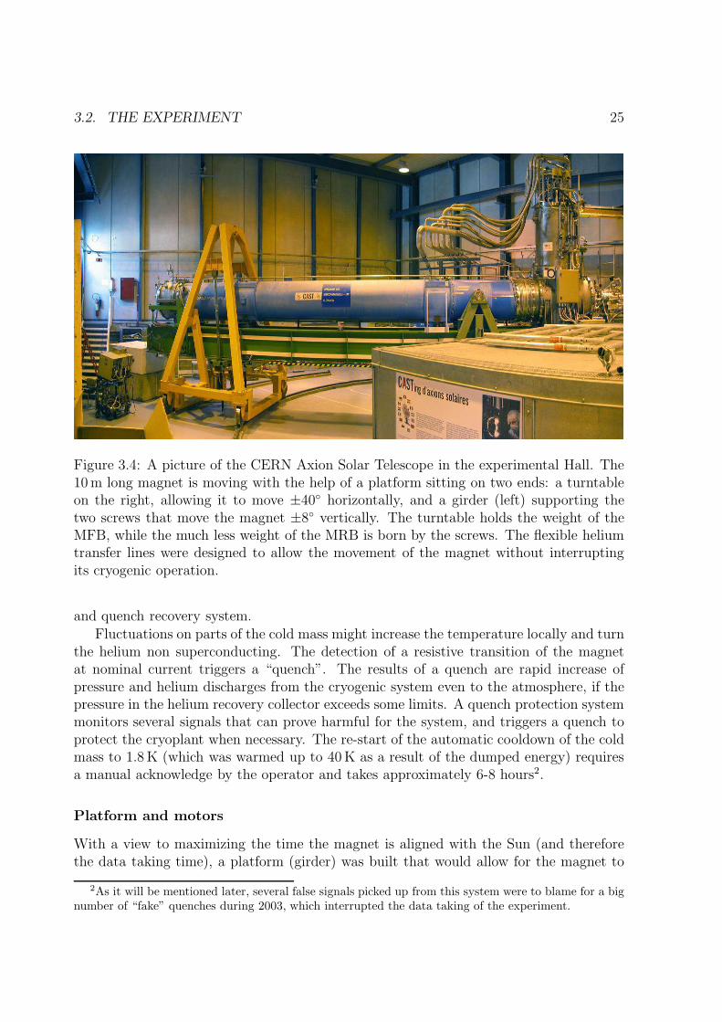
Figure 3.4: A picture of the CERN Axion Solar Telescope in the experimental Hall. The10 m long magnet is moving with the help of a platform sitting on two ends: a turntableon the right, allowing it to move ±40 horizontally, and a girder (left) supporting thetwo screws that move the magnet ±8 vertically. The turntable holds the weight of theMFB, while the much less weight of the MRB is born by the screws. The flexible heliumtransfer lines were designed to allow the movement of the magnet without interruptingits cryogenic operation.
and quench recovery system.Fluctuations on parts of the cold mass might increase the temperature locally and turn
the helium non superconducting. The detection of a resistive transition of the magnetat nominal current triggers a “quench”. The results of a quench are rapid increase ofpressure and helium discharges from the cryogenic system even to the atmosphere, if thepressure in the helium recovery collector exceeds some limits. A quench protection systemmonitors several signals that can prove harmful for the system, and triggers a quench toprotect the cryoplant when necessary. The re-start of the automatic cooldown of the coldmass to 1.8 K (which was warmed up to 40 K as a result of the dumped energy) requiresa manual acknowledge by the operator and takes approximately 6-8 hours2.
Platform and motors
With a view to maximizing the time the magnet is aligned with the Sun (and thereforethe data taking time), a platform (girder) was built that would allow for the magnet to
2As it will be mentioned later, several false signals picked up from this system were to blame for a bignumber of “fake” quenches during 2003, which interrupted the data taking of the experiment.
26 CHAPTER 3. THE CERN AXION SOLAR TELESCOPE EXPERIMENT
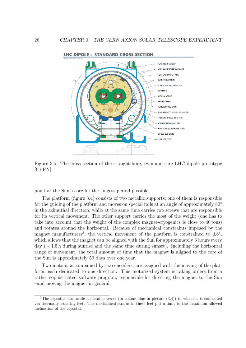
Figure 3.5: The cross section of the straight-bore, twin-aperture LHC dipole prototype[CERN].
point at the Sun’s core for the longest period possible.
The platform (figure 3.4) consists of two metallic supports; one of them is responsiblefor the guiding of the platform and moves on special rails at an angle of approximately 80
in the azimuthal direction, while at the same time carries two screws that are responsiblefor its vertical movement. The other support carries the most of the weight (one has totake into account that the weight of the complex magnet-cryogenics is close to 40 tons)and rotates around the horizontal. Because of mechanical constraints imposed by themagnet manufacturers3, the vertical movement of the platform is constrained to ±8,which allows that the magnet can be aligned with the Sun for approximately 3 hours everyday (∼ 1.5 h during sunrise and the same time during sunset). Including the horizontalrange of movement, the total amount of time that the magnet is aligned to the core ofthe Sun is approximately 50 days over one year.
Two motors, accompanied by two encoders, are assigned with the moving of the plat-form, each dedicated to one direction. This motorized system is taking orders from arather sophisticated software program, responsible for directing the magnet to the Sun–and moving the magnet in general.
3The cryostat sits inside a metallic vessel (in colour blue in picture (3.4)) to which it is connectedvia thermally isolating feet. The mechanical strains in these feet put a limit to the maximum allowedinclination of the cryostat.
3.2. THE EXPERIMENT 27
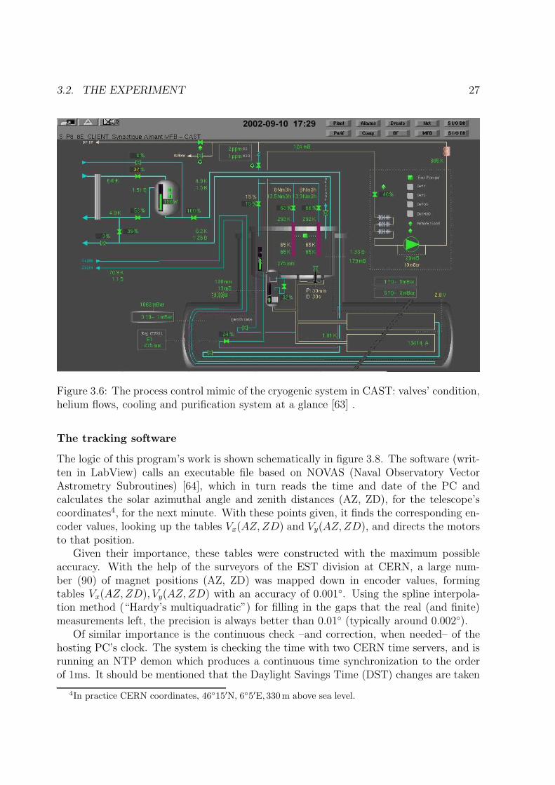
Figure 3.6: The process control mimic of the cryogenic system in CAST: valves’ condition,helium flows, cooling and purification system at a glance [63] .
The tracking software
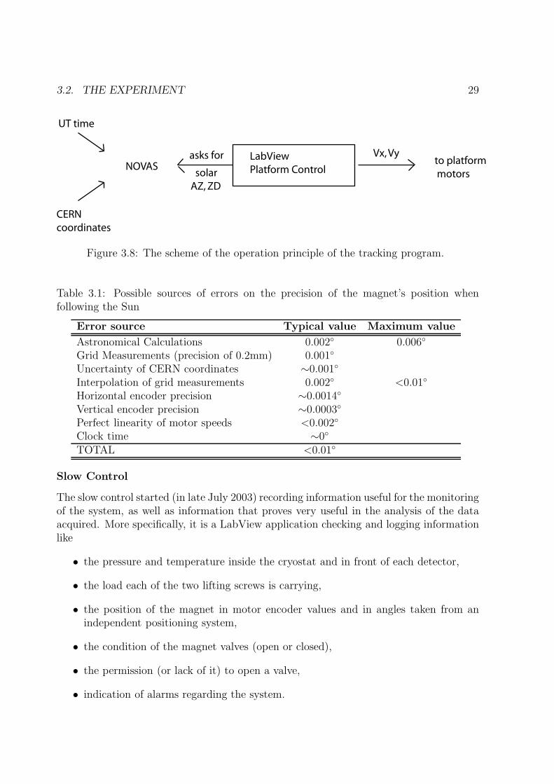
The logic of this program’s work is shown schematically in figure 3.8. The software (writ-ten in LabView) calls an executable file based on NOVAS (Naval Observatory VectorAstrometry Subroutines) [64], which in turn reads the time and date of the PC andcalculates the solar azimuthal angle and zenith distances (AZ, ZD), for the telescope’scoordinates4, for the next minute. With these points given, it finds the corresponding en-coder values, looking up the tables Vx(AZ,ZD) and Vy(AZ,ZD), and directs the motorsto that position.
Given their importance, these tables were constructed with the maximum possibleaccuracy. With the help of the surveyors of the EST division at CERN, a large num-ber (90) of magnet positions (AZ, ZD) was mapped down in encoder values, formingtables Vx(AZ,ZD), Vy(AZ,ZD) with an accuracy of 0.001. Using the spline interpola-tion method (“Hardy’s multiquadratic”) for filling in the gaps that the real (and finite)measurements left, the precision is always better than 0.01 (typically around 0.002).
Of similar importance is the continuous check –and correction, when needed– of thehosting PC’s clock. The system is checking the time with two CERN time servers, and isrunning an NTP demon which produces a continuous time synchronization to the orderof 1ms. It should be mentioned that the Daylight Savings Time (DST) changes are taken
4In practice CERN coordinates, 4615′N, 65′E, 330 m above sea level.

28 CHAPTER 3. THE CERN AXION SOLAR TELESCOPE EXPERIMENT
Figure 3.7: The flow scheme of the Magnet Feed Box (MFB) for the CAST experiment(taken from [63]).
into account in the executable .
Trying to sum up all possible error sources and their estimated values, Table 3.1 isformed.
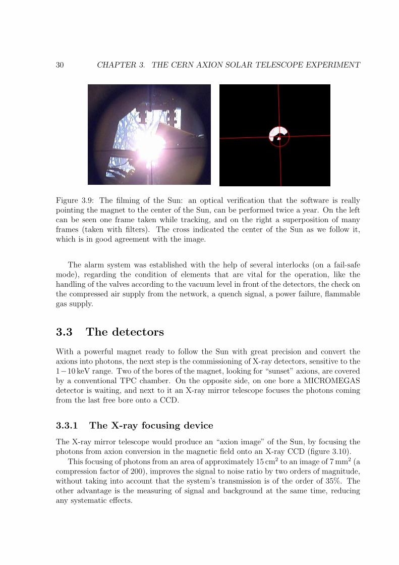
The table shows that the estimated precision is very good indeed for CAST. And yet,an image would be more eloquent. Despite the difficulties imposed by the location of thetelescope, optical verification of this precision is possible; an optical telescope is alignedwith the magnet axis and is coupled to a CCD camera. Twice a year, in mid-Marchand mid-September, when the Sun passes by a window specially made for this purposeand assuming that the weather permits it, the tracking software5 points the magnet tothe Sun, and the camera films during the movement. A close examination of the framesafterwards leads to a conclusion on the precision of the tracking (figure 3.9).
Apart from moving the magnet, the tracking software logs useful information like thetemperature in the experimental hall, the ambient pressure, the value of the intensity ofthe field inside the magnet. During the second year of operation, the recording of moreinformation was needed, therefore an independent slow control acquisition was used.
5In fact it is a second version of the tracking software, in which the refraction of light in the atmosphereis corrected for.
3.2. THE EXPERIMENT 29
asks for
solar
AZ, ZD
LabView
Platform Control
Vx, Vyto platform
motorsNOVAS
UT time
CERN
coordinates
Figure 3.8: The scheme of the operation principle of the tracking program.
Table 3.1: Possible sources of errors on the precision of the magnet’s position whenfollowing the Sun
Error source Typical value Maximum value
Astronomical Calculations 0.002 0.006
Grid Measurements (precision of 0.2mm) 0.001
Uncertainty of CERN coordinates ∼0.001
Interpolation of grid measurements 0.002 <0.01
Horizontal encoder precision ∼0.0014
Vertical encoder precision ∼0.0003
Perfect linearity of motor speeds <0.002
Clock time ∼0
TOTAL <0.01
Slow Control
The slow control started (in late July 2003) recording information useful for the monitoringof the system, as well as information that proves very useful in the analysis of the dataacquired. More specifically, it is a LabView application checking and logging informationlike
• the pressure and temperature inside the cryostat and in front of each detector,
• the load each of the two lifting screws is carrying,
• the position of the magnet in motor encoder values and in angles taken from anindependent positioning system,
• the condition of the magnet valves (open or closed),
• the permission (or lack of it) to open a valve,
• indication of alarms regarding the system.
30 CHAPTER 3. THE CERN AXION SOLAR TELESCOPE EXPERIMENT
Figure 3.9: The filming of the Sun: an optical verification that the software is reallypointing the magnet to the center of the Sun, can be performed twice a year. On the leftcan be seen one frame taken while tracking, and on the right a superposition of manyframes (taken with filters). The cross indicated the center of the Sun as we follow it,which is in good agreement with the image.
The alarm system was established with the help of several interlocks (on a fail-safemode), regarding the condition of elements that are vital for the operation, like thehandling of the valves according to the vacuum level in front of the detectors, the check onthe compressed air supply from the network, a quench signal, a power failure, flammablegas supply.
3.3 The detectors
With a powerful magnet ready to follow the Sun with great precision and convert theaxions into photons, the next step is the commissioning of X-ray detectors, sensitive to the1−10 keV range. Two of the bores of the magnet, looking for “sunset” axions, are coveredby a conventional TPC chamber. On the opposite side, on one bore a MICROMEGASdetector is waiting, and next to it an X-ray mirror telescope focuses the photons comingfrom the last free bore onto a CCD.
3.3.1 The X-ray focusing device
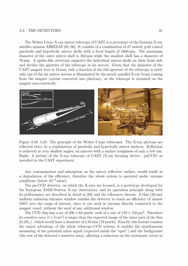
The X-ray mirror telescope would produce an “axion image” of the Sun, by focusing thephotons from axion conversion in the magnetic field onto an X-ray CCD (figure 3.10).
This focusing of photons from an area of approximately 15 cm2 to an image of 7 mm2 (acompression factor of 200), improves the signal to noise ratio by two orders of magnitude,without taking into account that the system’s transmission is of the order of 35%. Theother advantage is the measuring of signal and background at the same time, reducingany systematic effects.
3.3. THE DETECTORS 31
The Wolter I type X-ray mirror telescope of CAST is a prototype of the German X-raysatellite mission ABRIXAS [65, 66]. It consists of a combination of 27 nested, gold coatedparabolic and hyperbolic mirror shells with a focal length of 1600 mm. The maximumdiameter of the outer mirror shell is 163 mm while the smallest shell has a diameter of76 mm. A spider-like structure supports the individual mirror shells on their front sideand divides the aperture of the telescope in six sectors. Given that the diameter of theCAST magnet bore is 43 mm, only a fraction of the full aperture of the telescope is used;only one of the six mirror sectors is illuminated by the nearly parallel X-ray beam comingfrom the magnet (axions converted into photons), as the telescope is mounted on themagnet non-centrically.
Figure 3.10: Left: The principle of the Wolter I type telescopes. The X-ray photons arereflected twice by a combination of parabolic and hyperbolic mirror surfaces. Reflectionis achieved at very shallow angles, on mirrors with a surface roughness of only a few nm.Right: A picture of the X-ray telescope of CAST (X-ray focusing device - pnCCD) asinstalled in the CAST experiment.
Any contamination and adsorption on the mirror reflective surface, would result ina degradation of the efficiency, therefore the whole system is operated under vacuumconditions (below 10−5 mbar).
The pn-CCD detector, on which the X-rays are focused, is a prototype developed forthe European XMM-Newton X-ray observatory, and its operation principle along withits performance are described in detail in [68] and the references therein. A thin (20 nm)uniform radiation entrance window enables the detector to reach an efficiency of almost100% over the range of interest, since it can work in vacuum directly connected to themagnet vessel, without the need of any additional window.
The CCD chip has a set of 200× 64 pixels, each of a size of 150× 150µm2. Thereforeits sensitive area (1×3 cm2) is larger than the expected image of the inner part of the Sun(0.2R⊙) , which would have a diameter of 2.83 mm (19 pixels). Exactly this feature consiststhe major advantage of the whole telescope-CCD system; it enables the simultaneousmeasuring of the potential axion signal (expected inside the “spot”) and the background(the rest of the detector’s sensitive area), allowing a reduction on the systematic errors in
32 CHAPTER 3. THE CERN AXION SOLAR TELESCOPE EXPERIMENT
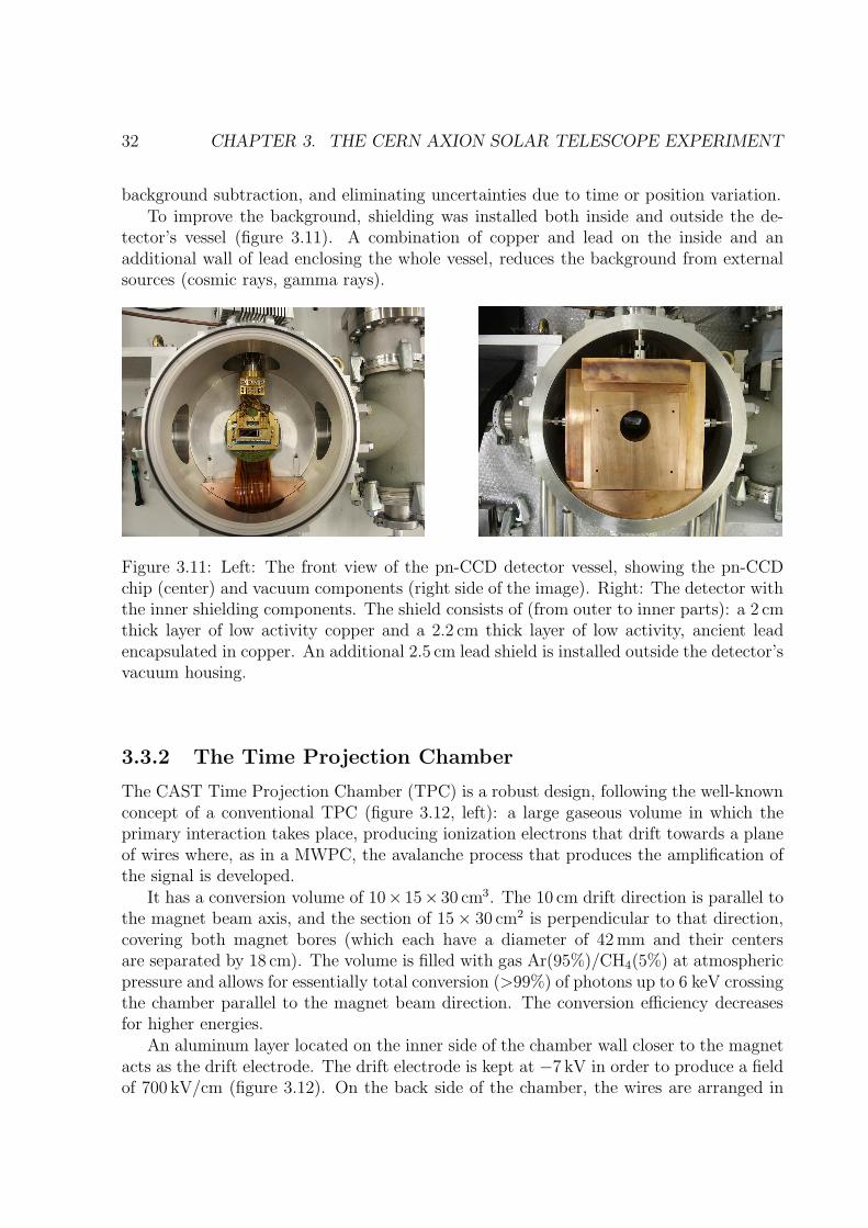
background subtraction, and eliminating uncertainties due to time or position variation.To improve the background, shielding was installed both inside and outside the de-
tector’s vessel (figure 3.11). A combination of copper and lead on the inside and anadditional wall of lead enclosing the whole vessel, reduces the background from externalsources (cosmic rays, gamma rays).
Figure 3.11: Left: The front view of the pn-CCD detector vessel, showing the pn-CCDchip (center) and vacuum components (right side of the image). Right: The detector withthe inner shielding components. The shield consists of (from outer to inner parts): a 2 cmthick layer of low activity copper and a 2.2 cm thick layer of low activity, ancient leadencapsulated in copper. An additional 2.5 cm lead shield is installed outside the detector’svacuum housing.
3.3.2 The Time Projection Chamber
The CAST Time Projection Chamber (TPC) is a robust design, following the well-knownconcept of a conventional TPC (figure 3.12, left): a large gaseous volume in which theprimary interaction takes place, producing ionization electrons that drift towards a planeof wires where, as in a MWPC, the avalanche process that produces the amplification ofthe signal is developed.
It has a conversion volume of 10× 15× 30 cm3. The 10 cm drift direction is parallel tothe magnet beam axis, and the section of 15 × 30 cm2 is perpendicular to that direction,covering both magnet bores (which each have a diameter of 42 mm and their centersare separated by 18 cm). The volume is filled with gas Ar(95%)/CH4(5%) at atmosphericpressure and allows for essentially total conversion (>99%) of photons up to 6 keV crossingthe chamber parallel to the magnet beam direction. The conversion efficiency decreasesfor higher energies.
An aluminum layer located on the inner side of the chamber wall closer to the magnetacts as the drift electrode. The drift electrode is kept at −7 kV in order to produce a fieldof 700 kV/cm (figure 3.12). On the back side of the chamber, the wires are arranged in

3.3. THE DETECTORS 33
Field shaping rings
Windows for X-Rays
Cathode planes of wires
Anode plane of wires
Figure 3.12: Left: A picture of the detector volume. Right: An exploded view of thedetector showing all its parts.
3 planes, one anode plane at +1.8 kV between two grounded cathode planes. The anodeplane contains 48 wires of 20µm diameter (gold plated tungsten), parallel to the wider sideof the chamber. Each cathode plane contains 96 wires of 100µm diameter, perpendicularto the anode wires. The distance between wires of the same plane is 3 mm. The distancebetween the anode and the cathode plane closest to the drift region is 3 mm, while thedistance between the anodes and the outer cathode plane is 6 mm. The avalanche processoccurs around the anode plane, due to the intense electric field, drawing the electronswhile the ions are gathered by the cathode planes, providing with the two-dimensionalposition information of the event.
Because of its low natural radioactivity, plexiglass was used to build the whole chamber(apart from the wires, the PCB board holding the wires and the screws that hold thechamber together). The thickness of the plexiglass is about 2 cm, except in three places(two on the back side and one on a lateral side) where the only separation between theinner gas and the atmosphere is a thin mylar foil to allow the calibration of the chamberwith low energy X-ray sources.
The detector is adjusted to the two magnet bores with the help of two very thin,alluminized (it serves as part of the drift electrode), mylar windows (3 or 5µm) stretchedon a metallic strongback on the side facing the magnet, in order to stand the pressuredifference between the detector volume and the magnet vacuum.
To reduce the background of the TPC, a shielding out of copper, lead, cadmium andpolyethylene was designed. Figure 3.13 shows a picture of the detector connected to themagnet, with part of the shielding mounted.

34 CHAPTER 3. THE CERN AXION SOLAR TELESCOPE EXPERIMENT
Figure 3.13: A picture of the TPC detector on the magnet; part of the shielding is built,allowing to see the copper box in which the detector is enclosed, the polyethylene wall,and in between the lead bricks.
3.3.3 MICROMEGAS
The fourth bore left, is covered by a MICROMEGAS detector (figure 3.14), which is goingto be described in detail in the next chapters.
Figure 3.14: A picture of the side of the CAST magnet were the MICROMEGAS detectoris attached.
3.4. COLLATERAL 35
3.4 Collateral
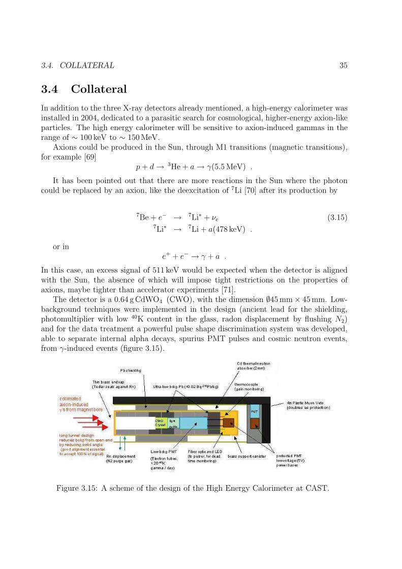
In addition to the three X-ray detectors already mentioned, a high-energy calorimeter wasinstalled in 2004, dedicated to a parasitic search for cosmological, higher-energy axion-likeparticles. The high energy calorimeter will be sensitive to axion-induced gammas in therange of ∼ 100 keV to ∼ 150 MeV.
Axions could be produced in the Sun, through M1 transitions (magnetic transitions),for example [69]
p+ d→ 3He + a→ γ(5.5 MeV) .
It has been pointed out that there are more reactions in the Sun where the photoncould be replaced by an axion, like the deexcitation of 7Li [70] after its production by
7Be + e− → 7Li∗ + νe (3.15)7Li∗ → 7Li + a(478 keV) .
or ine+ + e− → γ + a .
In this case, an excess signal of 511 keV would be expected when the detector is alignedwith the Sun, the absence of which will impose tight restrictions on the properties ofaxions, maybe tighter than accelerator experiments [71].
The detector is a 0.64 g CdWO4 (CWO), with the dimension ∅45 mm × 45 mm. Low-background techniques were implemented in the design (ancient lead for the shielding,photomultiplier with low 40K content in the glass, radon displacement by flushing N2)and for the data treatment a powerful pulse shape discrimination system was developed,able to separate internal alpha decays, spurius PMT pulses and cosmic neutron events,from γ-induced events (figure 3.15).
Figure 3.15: A scheme of the design of the High Energy Calorimeter at CAST.

36 CHAPTER 3. THE CERN AXION SOLAR TELESCOPE EXPERIMENT