A Semi-Analytic Model of Type Ia Supernovae

Kevin JumperAdvised by Dr. Robert Fisher

March 22, 2011

Review of Important Terms

• White Dwarf• Chandrasekhar Limit• Type Ia Supernovae• Flame Bubble– Self-Similarity

• Deflagration• Breakout• GCD Model

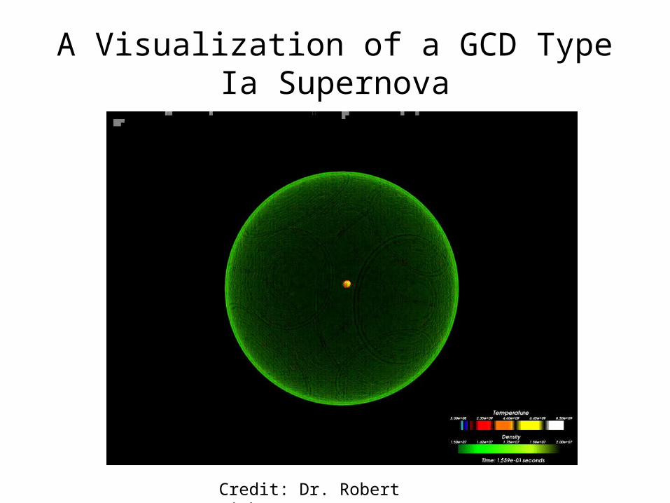
A Visualization of a GCD Type Ia Supernova

Credit: Dr. Robert Fisher

Project Objectives

• Determine the fractional mass burned during deflagration.

• Analyze the evolution of the flame bubble.

• Compare the results against other models and simulations.

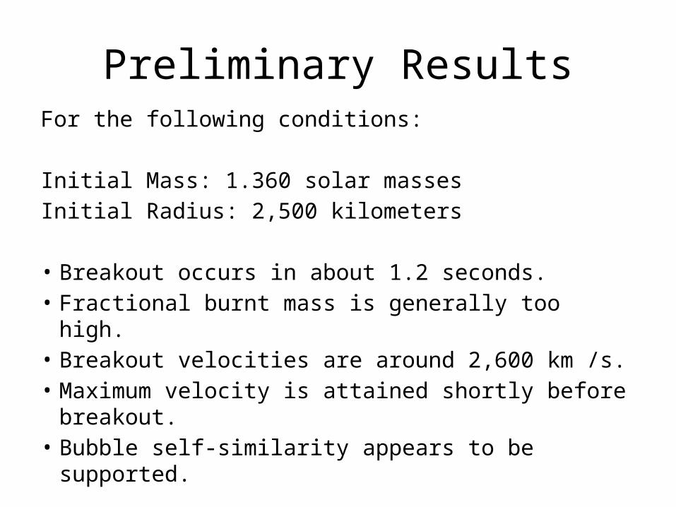
Preliminary ResultsFor the following conditions:

Initial Mass: 1.360 solar massesInitial Radius: 2,500 kilometers

• Breakout occurs in about 1.2 seconds.• Fractional burnt mass is generally too high.• Breakout velocities are around 2,600 km /s.• Maximum velocity is attained shortly before

breakout.• Bubble self-similarity appears to be supported.

Preliminary Results: Bubble-Self Similarity

• We saw the near-independence of breakout velocity from bubble conditions.

• This seemed to justify our spherical assumption for the model.

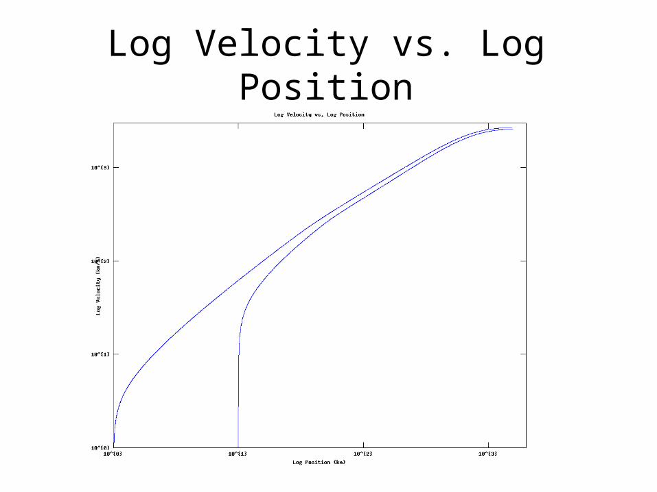
Log Velocity vs. Log Position

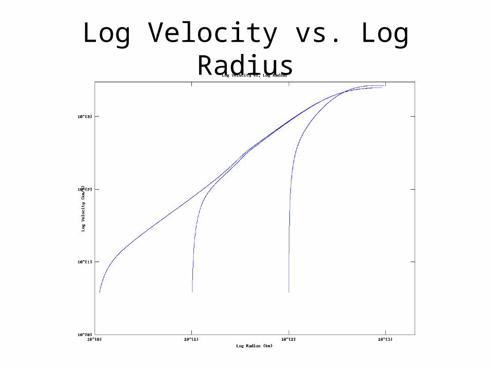
Log Velocity vs. Log Radius

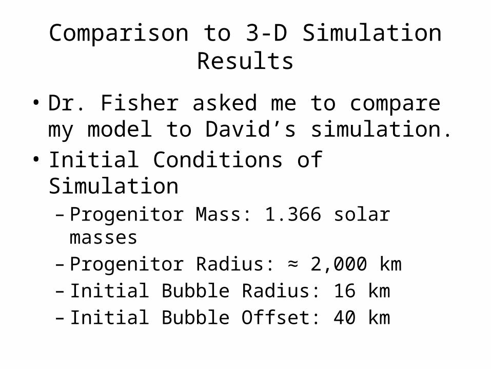
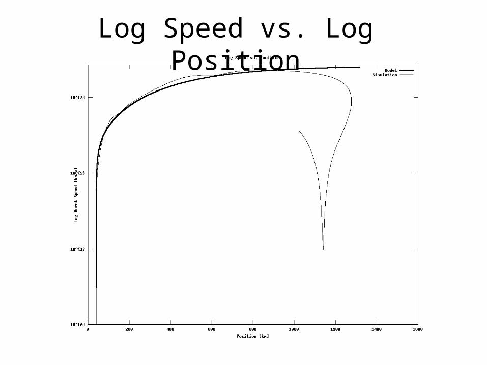
Comparison to 3-D Simulation Results

• Dr. Fisher asked me to compare my model to David’s simulation.

• Initial Conditions of Simulation– Progenitor Mass: 1.366 solar masses– Progenitor Radius: ≈ 2,000 km– Initial Bubble Radius: 16 km– Initial Bubble Offset: 40 km

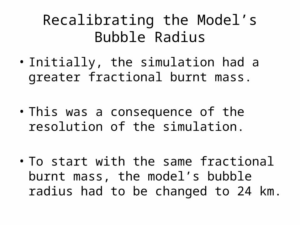
Recalibrating the Model’s Bubble Radius

• Initially, the simulation had a greater fractional burnt mass.

• This was a consequence of the resolution of the simulation.

• To start with the same fractional burnt mass, the model’s bubble radius had to be changed to 24 km.

Log Speed vs. Log Position

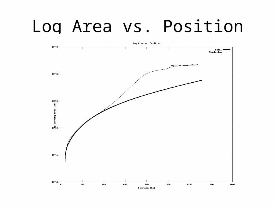
Log Area vs. Position

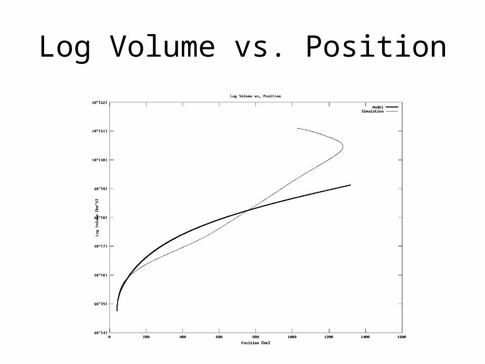
Log Volume vs. Position

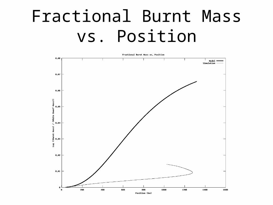
Fractional Burnt Mass vs. Position

Observations

• There is relatively good agreement with the simulation’s velocities.

• The area and volume diverge from the simulation over time.

• The model area and volume obey power laws.• There is a significant discrepancy between the

fractional burned mass of the model and simulation.

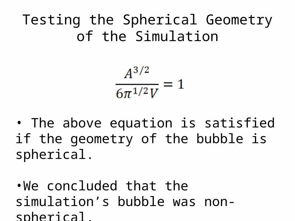
Testing the Spherical Geometry of the Simulation

• The above equation is satisfied if the geometry of the bubble is spherical.

•We concluded that the simulation’s bubble was non-spherical.

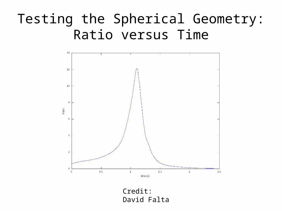
Testing the Spherical Geometry:Ratio versus Time

Credit: David Falta

Comparing to the Tabular Results

• The model’s code also has a routine to read in data about the progenitor instead of calculating it.

• However, the same general behavior as the semi-analytic model was observed.

• There was also a greater discrepancy in the fractional mass burnt.

Varying the Coefficient of Drag

• Dr. Fisher hypothesized that the coefficient of drag might be too high in the model.

• I was instructed to repeatedly halve the coefficient of drag and see if we could obtain the simulation’s fractional burnt mass.

• This is also affected by the Reynolds number, which describes turbulence.

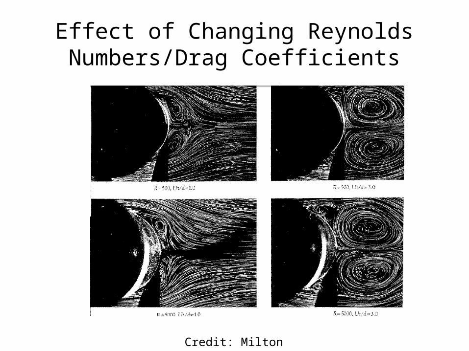
Effect of Changing Reynolds Numbers/Drag Coefficients

Credit: Milton van Dyke

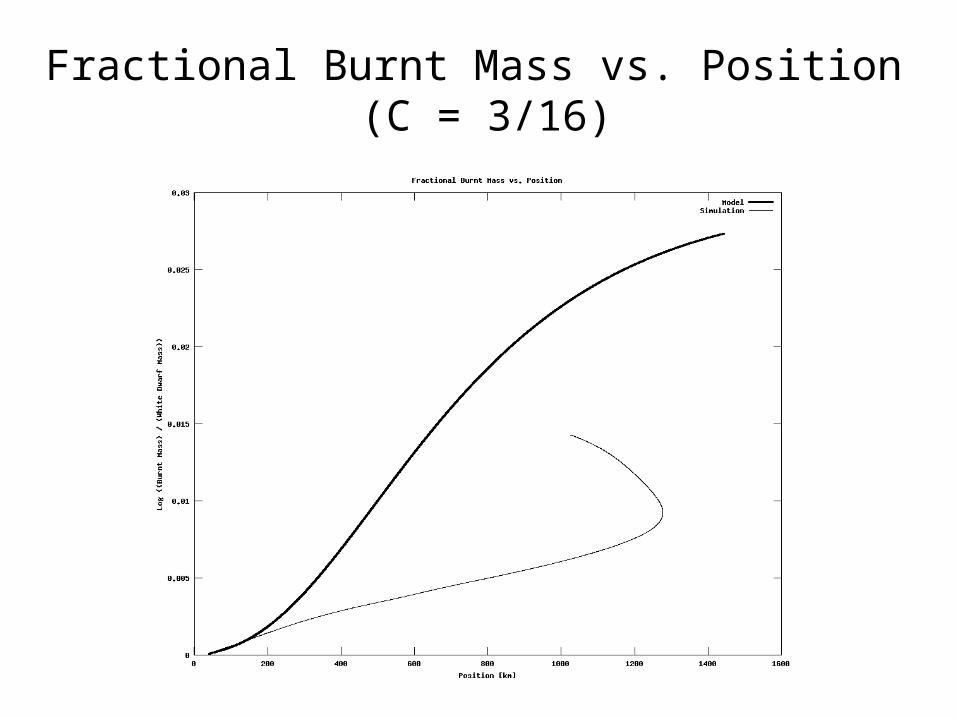
Fractional Burnt Mass vs. Position (C = 3/16)

Questions?

A Semi-Analytic Model of Type Ia Supernovae