A Signal-Processing Framework for Inverse RenderingRavi Ramamoorthi Pat Hanrahan

Stanford University ∗

Abstract

Realism in computer-generated images requires accurate inputmodels for lighting, textures and BRDFs. One of the best ways ofobtaining high-quality data is through measurements of scene at-tributes from real photographs by inverse rendering. However, in-verse rendering methods have been largely limited to settings withhighly controlled lighting. One of the reasons for this is the lackof a coherent mathematical framework for inverse rendering undergeneral illumination conditions. Our main contribution is the in-troduction of a signal-processing framework which describes thereflected light field as a convolution of the lighting and BRDF, andexpresses it mathematically as a product of spherical harmonic co-efficients of the BRDF and the lighting. Inverse rendering can thenbe viewed as deconvolution. We apply this theory to a variety ofproblems in inverse rendering, explaining a number of previous em-pirical results. We will show why certain problems are ill-posedor numerically ill-conditioned, and why other problems are moreamenable to solution. The theory developed here also leads to newpractical representations and algorithms. For instance, we presenta method to factor the lighting and BRDF from a small number ofviews, i.e. to estimate both simultaneously when neither is known.

CR Categories: I.3.7 [Computer Graphics]: Realism; I.4.8[Computer Vision]: Scene Analysis—Photometry

Keywords: Signal Processing, Spherical Harmonics, InverseRendering, Radiance, Light Field, Irradiance, Illumination, BRDF

1 Introduction

To create a realistic computer-generated image, we need bothan accurate, physically-based rendering algorithm and a detailedmodel of the scene including light sources and objects specifiedby their geometry and material properties—texture and reflectance(BRDF). There has been substantial progress in the developmentof rendering algorithms, and nowadays, realism is often limited bythe quality of input models. As a result, image-based rendering isbecoming widespread. In its simplest form, image-based render-ing uses view interpolation to construct new images from acquiredimages without constructing a conventional scene model.

The quality of view interpolation may be significantly improvedif it is coupled with inverse rendering. Inverse rendering mea-sures rendering attributes—lighting, textures, and BRDF—fromphotographs. Whether traditional or image-based rendering algo-rithms are used, rendered images use measurements from real ob-jects, and therefore appear very similar to real scenes. Measur-ing scene attributes also introduces structure into the raw imagery,making it easier to manipulate the scene. For example, an artist canchange independently the material properties or the lighting.

Inverse rendering methods such as those of Debevec et al. [6],Marschner et al. [21], and Sato et al. [32], have produced high

∗(ravir,hanrahan)@graphics.stanford.edu

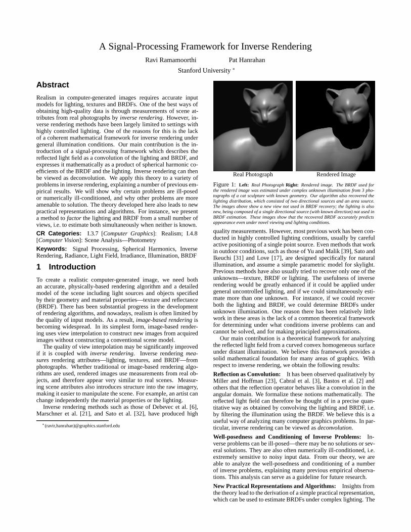
Real Photograph Rendered Image

Figure 1: Left: Real Photograph Right: Rendered image. The BRDF used forthe rendered image was estimated under complex unknown illumination from 3 pho-tographs of a cat sculpture with known geometry. Our algorithm also recovered thelighting distribution, which consisted of two directional sources and an area source.The images above show a new view not used in BRDF recovery; the lighting is alsonew, being composed of a single directional source (with known direction) not used inBRDF estimation. These images show that the recovered BRDF accurately predictsappearance even under novel viewing and lighting conditions.

quality measurements. However, most previous work has been con-ducted in highly controlled lighting conditions, usually by carefulactive positioning of a single point source. Even methods that workin outdoor conditions, such as those of Yu and Malik [39], Sato andIkeuchi [31] and Love [17], are designed specifically for naturalillumination, and assume a simple parametric model for skylight.Previous methods have also usually tried to recover only one of theunknowns—texture, BRDF or lighting. The usefulness of inverserendering would be greatly enhanced if it could be applied undergeneral uncontrolled lighting, and if we could simultaneously esti-mate more than one unknown. For instance, if we could recoverboth the lighting and BRDF, we could determine BRDFs underunknown illumination. One reason there has been relatively littlework in these areas is the lack of a common theoretical frameworkfor determining under what conditions inverse problems can andcannot be solved, and for making principled approximations.

Our main contribution is a theoretical framework for analyzingthe reflected light field from a curved convex homogeneous surfaceunder distant illumination. We believe this framework provides asolid mathematical foundation for many areas of graphics. Withrespect to inverse rendering, we obtain the following results:

Reflection as Convolution: It has been observed qualitatively byMiller and Hoffman [23], Cabral et al. [3], Bastos et al. [2] andothers that the reflection operator behaves like a convolution in theangular domain. We formalize these notions mathematically. Thereflected light field can therefore be thought of in a precise quan-titative way as obtained by convolving the lighting and BRDF, i.e.by filtering the illumination using the BRDF. We believe this is auseful way of analyzing many computer graphics problems. In par-ticular, inverse rendering can be viewed as deconvolution.

Well-posedness and Conditioning of Inverse Problems: In-verse problems can be ill-posed—there may be no solutions or sev-eral solutions. They are also often numerically ill-conditioned, i.e.extremely sensitive to noisy input data. From our theory, we areable to analyze the well-posedness and conditioning of a numberof inverse problems, explaining many previous empirical observa-tions. This analysis can serve as a guideline for future research.

New Practical Representations and Algorithms: Insights fromthe theory lead to the derivation of a simple practical representation,which can be used to estimate BRDFs under complex lighting. The

theory also leads to novel frequency space and hybrid angular andfrequency space methods for inverse problems, including two newalgorithms for estimating the lighting, and an algorithm for simul-taneously determining the lighting and BRDF. Therefore, we canrecover BRDFs under general, unknown lighting conditions.

2 Previous Work

To describe previous work, we will introduce a taxonomy based onhow many of the three quantities—lighting, BRDF and texture—are unknown. To motivate the taxonomy, we first write a simplifiedversion of the reflection equation, omitting visibility.

B(x, ωo) =

ZΩi

T (x)ρ(ωi, ωo)L(x, ωi)(ωi · n) dωi (1)

Here, B is the reflected light field, expressed as a function of thesurface position x and outgoing direction ωo. The normal vector isn. For simplicity, we assume that a single texture T modulates theBRDF. In practice, we would use separate textures for the diffuseand specular components of the BRDF.

The integrand is a product of terms—the texture T (x), theBRDF ρ(ωi, ωo), and the lighting L(x, ωi). Inverse rendering, as-suming known geometry, involves inverting the integral to recoverone or more of ρ, L, or T . If two or more quantities are unknown,inverse rendering involves factoring the reflected light field.

One Unknown

1. Unknown Texture: Previous methods have recovered thediffuse texture of a surface using a single point light source bydividing by the irradiance in order to estimate the albedo at eachpoint. Details are given by Marschner [34] and Levoy et al. [16].

2. Unknown BRDF: The BRDF [24] is a fundamental intrinsicsurface property. Active measurement methods, known as goniore-flectometry, involving a single point source and a single observa-tion at a time, have been developed. Improvements are suggestedby Ward [37] and Karner et al. [12]. More recently, image-basedBRDF measurement methods have been proposed by Lu et al. [18]and Marschner et al. [21]. If the entire BRDF is measured, it may berepresented by tabulating its values. An alternative representationis by low-parameter models such as those of Ward [37] or Torranceand Sparrow [36]. The parametric BRDF will generally not be asaccurate as a full measured BRDF. However, parametric models areoften preferred in practice since they are compact, and are simplerto estimate. Love [17] estimates parametric BRDFs under natu-ral illumination, assuming a low-parameter model for skylight andsunlight. Dror et al. [7] classify the surface reflectance as one ofa small number of predetermined BRDFs, making use of assumedstatistical characteristics of natural lighting. However, the inverseBRDF problem has not been solved for general illumination.

3. Unknown Lighting: A common solution is to use a mirroredball, as done by Miller and Hoffman [23]. Marschner and Green-berg [20] find the lighting from a Lambertian surface. D’Zmura [8]proposes, but does not demonstrate, estimating spherical harmoniccoefficients. For Lambertian objects, we [29] have shown how torecover the first 9 spherical harmonics. Previous work has not esti-mated the lighting from curved surfaces with general BRDFs.

Two Unknowns

4. Factorization—Unknown Lighting and BRDF: BRDFestimation methods have been proposed by Ikeuchi and Sato [10]and Tominaga and Tanaka [35] for the special case when the light-ing consists of a single source of unknown direction. However,these methods cannot simultaneously recover a complex lightingdistribution and the object BRDF. One of the main practical con-tributions of this paper is a solution to this problem for curved sur-faces, allowing us to estimate BRDFs under general unknown illu-mination, while also determining the lighting. The closest previouswork is that of Sato et al. [30] who use shadows to estimate theillumination distribution and the surface reflectance properties. We

extend this work by not requiring shadow information, and present-ing improved methods for estimating the illumination.

5. Factorization—Unknown Texture and BRDF: This cor-responds to recovering textured, or spatially-varying BRDFs. Satoet al. [32] rotate an object on a turntable, using a single pointsource, to recover BRDF parameters and texture. Yu et al. [38] re-cover a texture only for the diffuse BRDF component, but accountfor interreflections. Using a large number of images obtained bymoving a point source around a sphere surrounding the subject,Debevec et al. [6] acquire the reflectance field of a human face,and recover parameters of a microfacet BRDF model for each sur-face location. Sato and Ikeuchi [31] and Yu and Malik [39] recoverBRDFs and diffuse textures under natural illumination, assuminga simple parametric model for skylight, and using a sequence ofimages acquired under different illumination conditions. Most ofthese methods recover only diffuse textures; constant values, orrelatively low-resolution textures, are used for the specular param-eters. A notable exception is the work of Dana et al. [5] who gen-eralize BRDFs to a 6D bi-directional texture function (BTF).

6. Factorization—Unknown Lighting and Texture: Wehave shown [29] that a distant illumination field can cause only lowfrequency variation in the radiosity of a convex Lambertian sur-face. This implies that, for a diffuse object, high-frequency texturecan be recovered independently of lighting. These observations arein agreement with the perception literature, such as Land’s retinextheory [15], wherein high-frequency variation is usually attributedto texture, and low-frequency variation associated with illumina-tion. However, note that there is a fundamental ambiguity betweenlow-frequency texture and lighting effects. Therefore, lighting andtexture cannot be factored without using active methods or makingfurther assumptions regarding their expected characteristics.

General Case: Three Unknowns

7. Factorization—Unknown Lighting, Texture, BRDF:Ultimately, we wish to recover textured BRDFs under unknownlighting. We cannot solve this problem without further assump-tions, because we must first resolve the lighting-texture ambiguity.

Our approach differs from previous work in that it is derivedfrom a mathematical theory of inverse rendering. As such, it hassimilarities to inverse methods used in areas of radiative transferand transport theory such as hydrologic optics [26] and neutronscattering. See McCormick [22] for a review.

In previous theoretical work, D’Zmura [8] has analyzed reflec-tion as a linear operator in terms of spherical harmonics, and dis-cussed some resulting perceptual ambiguities between reflectanceand illumination. In computer graphics, Cabral et al. [3] firstdemonstrated the use of spherical harmonics to represent BRDFs.We extend these methods by explicitly deriving the frequency-space reflection equation (i.e. convolution formula), and by provid-ing quantitative results for various special cases. We have earlier re-ported on theoretical results for planar or flatland light fields [27],and for determining the lighting from a Lambertian surface [29].For the Lambertian case, similar results have been derived inde-pendently by Basri and Jacobs [1] in simultaneous work on facerecognition. This paper extends these previous results to the gen-eral 3D case with arbitrary isotropic BRDFs, and applies the theoryto developing new practical inverse-rendering algorithms.

3 Assumptions

The input to our algorithms consists of object geometry and pho-tographs from a number of different locations, with known extrinsicand intrinsic camera parameters. We assume static scenes, i.e. thatthe object remains stationary and the lighting remains the same be-tween views. Our method is a passive-vision approach; we do notactively disturb the environment. Our assumptions are:

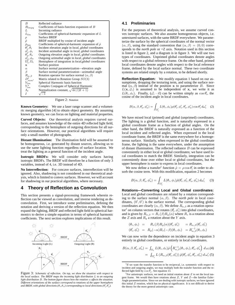
B Reflected radianceBlmpq Coefficients of basis-function expansion of BL Incoming radianceLlm Coefficients of spherical-harmonic expansion of Lρ Surface BRDFρ BRDF multiplied by cosine of incident angleρlpq Coefficients of spherical-harmonic expansion of ρθ′i, θi Incident elevation angle in local, global coordinatesφ′

i, φi Incident azimuthal angle in local, global coordinatesθ′o, θo Outgoing elevation angle in local, global coordinatesφ′

o, φo Outgoing azimuthal angle in local, global coordinatesΩ′

i,Ωi Hemisphere of integration in local,global coordinatesx Surface positionα Surface normal parameterization—elevation angleβ Surface normal parameterization—azimuthal angleRα,β Rotation operator for surface normal (α, β)Dl

mm′ Matrix related to Rotation Group SO(3)Ylm Spherical Harmonic basis functionY ∗

lm Complex Conjugate of Spherical HarmonicΛl Normalization constant,

p4π/(2l + 1)

I√−1

Figure 2: Notation

Known Geometry: We use a laser range scanner and a volumet-ric merging algorithm [4] to obtain object geometry. By assumingknown geometry, we can focus on lighting and material properties.

Curved Objects: Our theoretical analysis requires curved sur-faces, and assumes knowledge of the entire 4D reflected light field,corresponding to the hemisphere of outgoing directions for all sur-face orientations. However, our practical algorithms will requireonly a small number of photographs.

Distant Illumination: The illumination field will be assumed tobe homogeneous, i.e. generated by distant sources, allowing us touse the same lighting function regardless of surface location. Wetreat the lighting as a general function of the incident angle.

Isotropic BRDFs: We will consider only surfaces havingisotropic BRDFs. The BRDF will therefore be a function of only 3variables, instead of 4, i.e. 3D instead of 4D.

No Interreflection: For concave surfaces, interreflection will beignored. Also, shadowing is not considered in our theoretical anal-ysis, which is limited to convex surfaces. However, we will accountfor shadowing in our practical algorithms, where necessary.

4 Theory of Reflection as Convolution

This section presents a signal-processing framework wherein re-flection can be viewed as convolution, and inverse rendering as de-convolution. First, we introduce some preliminaries, defining thenotation and deriving a version of the reflection equation. We thenexpand the lighting, BRDF and reflected light field in spherical har-monics to derive a simple equation in terms of spherical harmoniccoefficients. The next section explores implications of this result.

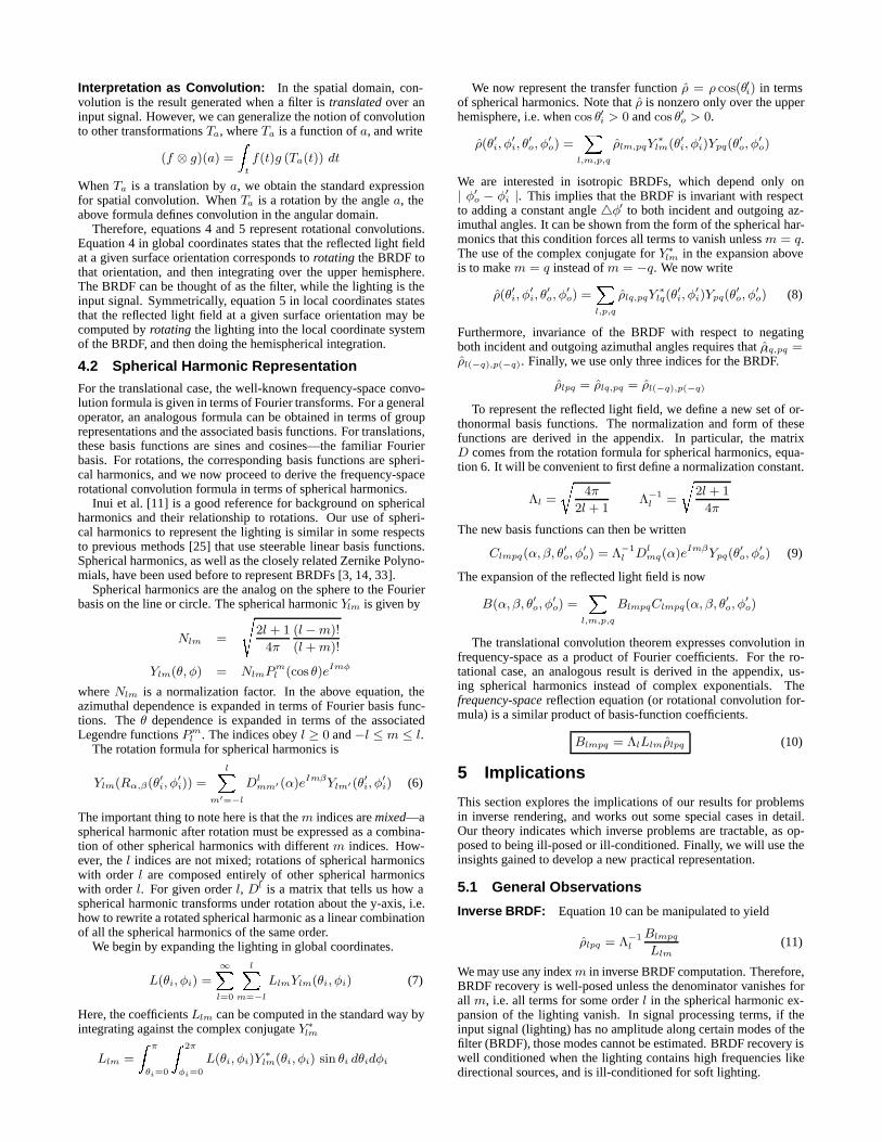
Incoming Light (L) Outgoing Light (B)

α α

BRDF

iθ

iθ

BRDF

’o’θ

oθ

’ o’θiθ

Figure 3: Schematic of reflection. On top, we show the situation with respect tothe local surface. The BRDF maps the incoming light distribution L to an outgoinglight distributionB. The bottom figure shows how the rotation α affects the situation.Different orientations of the surface correspond to rotations of the upper hemisphereand BRDF, with global directions (θi,θo) corresponding to local directions (θ′i ,θ′o).

4.1 Preliminaries

For the purposes of theoretical analysis, we assume curved con-vex isotropic surfaces. We also assume homogeneous objects, i.e.untextured surfaces, with the same BRDF everywhere. We parame-terize the surface by the spherical coordinates of the normal vector(α, β), using the standard convention that (α, β) = (0, 0) corre-sponds to the north pole or +Z axis. Notation used in this sectionis listed in figure 2, and a diagram is in figure 3. We will use twotypes of coordinates. Unprimed global coordinates denote angleswith respect to a global reference frame. On the other hand, primedlocal coordinates denote angles with respect to the local referenceframe, defined by the local surface normal. These two coordinatesystems are related simply by a rotation, to be defined shortly.

Reflection Equation: We modify equation 1 based on our as-sumptions, dropping the texturing term, and using the surface nor-mal (α, β) instead of the position x to parameterize B. SinceL(x, ωi) is assumed to be independent of x, we write it asL(θi, φi). Finally, ( ωi · n) can be written simply as cos θ′i, thecosine of the incident angle in local coordinates.

B(α, β, θ′o, φ′o) =

ZΩ′

i

L(θi, φi)ρ(θ′i, φ′i, θ

′o, φ′

o) cos θ′i dω′i (2)

We have mixed local (primed) and global (unprimed) coordinates.The lighting is a global function, and is naturally expressed in aglobal coordinate frame as a function of global angles. On theother hand, the BRDF is naturally expressed as a function of thelocal incident and reflected angles. When expressed in the localcoordinate frame, the BRDF is the same everywhere for a homoge-neous surface. Similarly, when expressed in the global coordinateframe, the lighting is the same everywhere, under the assumptionof distant illumination. The reflected radiance B can be expressedconveniently in either local or global coordinates; we have used lo-cal coordinates to match the BRDF. Similarly, integration can beconveniently done over either local or global coordinates, but theupper hemisphere is easier to express in local coordinates.

We now define a transfer1 function ρ = ρ cos θ′i in order to ab-sorb the cosine term. With this modification, equation 2 becomes

B(α, β, θ′o, φ′o) =

ZΩ′

i

L(θi, φi)ρ(θ′i, φ

′i, θ

′o, φ

′o) dω

′i (3)

Rotations—Converting Local and Global coordinates:Local and global coordinates are related by a rotation correspond-ing to the surface normal (α, β). The north pole in local coor-dinates, (0′, 0′) is the surface normal. The corresponding globalcoordinates are clearly (α, β). We define Rα,β as a rotation opera-tor2 on column vectors that rotates (θ′i, φ

′i) into global coordinates,

and is given by Rα,β = Rz(β)Ry(α) where Rz is a rotation aboutthe Z axis and Ry a rotation about the Y axis.

(θi, φi) = Rz(β)Ry(α)(θ′i, φ′i) = Rα,β(θ′i, φ

′i)

(θ′i, φ′i) = Ry(−α)Rz(−β)(θi, φi) = R−1

α,β(θi, φi)

We can now write the dependence on incident angle in equation 3entirely in global coordinates, or entirely in local coordinates.

B(α, β, θ′o, φ′o) =

RΩi

L(θi, φi)ρR−1

α,β(θi, φi), θ′o, φ

′o

dωi (4)

=RΩ′

iL (Rα,β(θ′i, φ

′i)) ρ(θ

′i, φ

′i, θ

′o, φ

′o) dω

′i (5)

1If we want the transfer function to be reciprocal, i.e. symmetric with respect toincident and outgoing angles, we may multiply both the transfer function and the re-flected light field by cos θ′o. See equation 13.

2For anisotropic surfaces, we need an initial rotation about Z to set the local tan-gent frame. We would then have rotations about Z, Y and Z—the familiar Euler-Angle parameterization. Since we are dealing with isotropic surfaces, we have ignoredthis initial Z rotation, which has no physical significance. It is not difficult to derivethe theory for the more general anisotropic case.

Interpretation as Convolution: In the spatial domain, con-volution is the result generated when a filter is translated over aninput signal. However, we can generalize the notion of convolutionto other transformations Ta, where Ta is a function of a, and write

(f ⊗ g)(a) =

Zt

f(t)g (Ta(t)) dt

When Ta is a translation by a, we obtain the standard expressionfor spatial convolution. When Ta is a rotation by the angle a, theabove formula defines convolution in the angular domain.

Therefore, equations 4 and 5 represent rotational convolutions.Equation 4 in global coordinates states that the reflected light fieldat a given surface orientation corresponds to rotating the BRDF tothat orientation, and then integrating over the upper hemisphere.The BRDF can be thought of as the filter, while the lighting is theinput signal. Symmetrically, equation 5 in local coordinates statesthat the reflected light field at a given surface orientation may becomputed by rotating the lighting into the local coordinate systemof the BRDF, and then doing the hemispherical integration.

4.2 Spherical Harmonic Representation

For the translational case, the well-known frequency-space convo-lution formula is given in terms of Fourier transforms. For a generaloperator, an analogous formula can be obtained in terms of grouprepresentations and the associated basis functions. For translations,these basis functions are sines and cosines—the familiar Fourierbasis. For rotations, the corresponding basis functions are spheri-cal harmonics, and we now proceed to derive the frequency-spacerotational convolution formula in terms of spherical harmonics.

Inui et al. [11] is a good reference for background on sphericalharmonics and their relationship to rotations. Our use of spheri-cal harmonics to represent the lighting is similar in some respectsto previous methods [25] that use steerable linear basis functions.Spherical harmonics, as well as the closely related Zernike Polyno-mials, have been used before to represent BRDFs [3, 14, 33].

Spherical harmonics are the analog on the sphere to the Fourierbasis on the line or circle. The spherical harmonic Ylm is given by

Nlm =

s2l + 1

4π

(l−m)!

(l + m)!

Ylm(θ, φ) = NlmPml (cos θ)eImφ

where Nlm is a normalization factor. In the above equation, theazimuthal dependence is expanded in terms of Fourier basis func-tions. The θ dependence is expanded in terms of the associatedLegendre functions Pm

l . The indices obey l ≥ 0 and −l ≤ m ≤ l.The rotation formula for spherical harmonics is

Ylm(Rα,β(θ′i, φ′i)) =

lXm′=−l

Dlmm′ (α)eImβYlm′(θ′i, φ

′i) (6)

The important thing to note here is that the m indices are mixed—aspherical harmonic after rotation must be expressed as a combina-tion of other spherical harmonics with different m indices. How-ever, the l indices are not mixed; rotations of spherical harmonicswith order l are composed entirely of other spherical harmonicswith order l. For given order l, Dl is a matrix that tells us how aspherical harmonic transforms under rotation about the y-axis, i.e.how to rewrite a rotated spherical harmonic as a linear combinationof all the spherical harmonics of the same order.

We begin by expanding the lighting in global coordinates.

L(θi, φi) =∞X

l=0

lXm=−l

LlmYlm(θi, φi) (7)

Here, the coefficients Llm can be computed in the standard way byintegrating against the complex conjugate Y∗

lm

Llm =

Z π

θi=0

Z 2π

φi=0

L(θi, φi)Y∗

lm(θi, φi) sin θi dθidφi

We now represent the transfer function ρ = ρ cos(θ′i) in termsof spherical harmonics. Note that ρ is nonzero only over the upperhemisphere, i.e. when cos θ′i > 0 and cos θ′o > 0.

ρ(θ′i, φ′i, θ

′o, φ

′o) =

Xl,m,p,q

ρlm,pqY∗

lm(θ′i, φ′i)Ypq(θ

′o, φ

′o)

We are interested in isotropic BRDFs, which depend only on| φ′

o − φ′i |. This implies that the BRDF is invariant with respect

to adding a constant angle φ′ to both incident and outgoing az-imuthal angles. It can be shown from the form of the spherical har-monics that this condition forces all terms to vanish unless m = q.The use of the complex conjugate for Y∗

lm in the expansion aboveis to make m = q instead of m = −q. We now write

ρ(θ′i, φ′i, θ

′o, φ

′o) =

Xl,p,q

ρlq,pqY∗

lq(θ′i, φ

′i)Ypq(θ

′o, φ

′o) (8)

Furthermore, invariance of the BRDF with respect to negatingboth incident and outgoing azimuthal angles requires that ρlq,pq =ρl(−q),p(−q). Finally, we use only three indices for the BRDF.

ρlpq = ρlq,pq = ρl(−q),p(−q)

To represent the reflected light field, we define a new set of or-thonormal basis functions. The normalization and form of thesefunctions are derived in the appendix. In particular, the matrixD comes from the rotation formula for spherical harmonics, equa-tion 6. It will be convenient to first define a normalization constant.

Λl =

r4π

2l + 1Λ−1

l =

r2l + 1

4π

The new basis functions can then be written

Clmpq(α, β, θ′o, φ

′o) = Λ−1

l Dlmq(α)eImβYpq(θ

′o, φ

′o) (9)

The expansion of the reflected light field is now

B(α, β, θ′o, φ′o) =

Xl,m,p,q

BlmpqClmpq(α, β, θ′o, φ

′o)

The translational convolution theorem expresses convolution infrequency-space as a product of Fourier coefficients. For the ro-tational case, an analogous result is derived in the appendix, us-ing spherical harmonics instead of complex exponentials. Thefrequency-space reflection equation (or rotational convolution for-mula) is a similar product of basis-function coefficients.

Blmpq = ΛlLlmρlpq (10)

5 Implications

This section explores the implications of our results for problemsin inverse rendering, and works out some special cases in detail.Our theory indicates which inverse problems are tractable, as op-posed to being ill-posed or ill-conditioned. Finally, we will use theinsights gained to develop a new practical representation.

5.1 General Observations

Inverse BRDF: Equation 10 can be manipulated to yield

ρlpq = Λ−1l

Blmpq

Llm(11)

We may use any index m in inverse BRDF computation. Therefore,BRDF recovery is well-posed unless the denominator vanishes forall m, i.e. all terms for some order l in the spherical harmonic ex-pansion of the lighting vanish. In signal processing terms, if theinput signal (lighting) has no amplitude along certain modes of thefilter (BRDF), those modes cannot be estimated. BRDF recovery iswell conditioned when the lighting contains high frequencies likedirectional sources, and is ill-conditioned for soft lighting.

Inverse Lighting: Equation 10 can also be manipulated to yield

Llm = Λ−1l

Blmpq

ρlpq(12)

Similarly as for BRDF recovery, any p, q can be used for inverselighting. The problem is well-posed unless the denominator ρlpq

vanishes for all p, q for some l. In signal processing terms, whenthe BRDF filter truncates certain frequencies in the input lightingsignal (for instance, if it were a low-pass filter), we cannot deter-mine those frequencies from the output signal. Inverse lighting iswell-conditioned when the BRDF has high-frequency componentslike sharp specularities, and is ill-conditioned for diffuse surfaces.Light Field Factorization—Lighting and BRDF: We nowconsider the problem of factorizing the light field, i.e simultane-ously recovering the lighting and BRDF when both are unknown.The reflected light field is defined on a four-dimensional domainwhile the lighting is a function of two dimensions and the isotropicBRDF is defined on a three-dimensional domain. This seems to in-dicate that we have more knowns (in terms of coefficients of the re-flected light field) than unknowns (lighting and BRDF coefficients).

For fixed order l, we can use known lighting coefficients Llm

to find unknown BRDF coefficients ρlpq and vice-versa. In fact,we need only one known nonzero lighting or BRDF coefficient tobootstrap this process. It would appear from equation 10, however,that there is an unrecoverable scale factor for each order l, corre-sponding to the known coefficient we require. But, we can also usereciprocity of the BRDF. To make the transfer function symmetric,we multiply it, as well as the reflected light field B, by cos θ′o.

ρ = ρ cos θ′o = ρ cos θ′i cos θ′o

B = B cos θ′o

Blmpq = ΛlLlmρlpq (13)The new transfer function ρ is symmetric with respect to incidentand outgoing directions, and corresponding indices: ρlpq = ρplq.

There is a global scale factor we cannot recover, since B is notaffected if we multiply the lighting and divide the BRDF by thesame amount. Therefore, we scale the lighting so the DC termL00 = Λ−1

0 =p

1/ (4π). Now, using equations 11, 12, and 13,

L00 = Λ−10

ρ0p0 = B00p0

Llm = Λ−1l

Blmpq

ρlpq=

Blm00

ρl00=

Blm00

ρ0l0

= Λ−1l

Blm00

B00l0

ρlpq = Λ−1l

Blmpq

Llm

=BlmpqB00l0

Blm00

In the last line, we can use any value of m. This gives an explicitformula for the lighting and BRDF in terms of coefficients of theoutput light field. Therefore, up to global scale, the reflected lightfield can be factored into the lighting and the BRDF, providedthe appropriate coefficients of the reflected light field do not vanish.

5.2 Special Cases

Mirror BRDF: The mirror BRDF corresponds to a gazingsphere. Just as the inverse lighting problem is easily solved in angu-lar space in this case, we will show that it is well-posed and easilysolved in frequency space. The BRDF involves a delta function,

ρ(θ′i, φ′i, θ

′o, φ

′o) = δ(cos θ′i − cos θ′o)δ(φ

′i − φ′

o ± π)

Note that the BRDF is nonzero only when θ′i ≤ π/2 and θ′o ≤ π/2.The coefficients for the BRDF, reflected light field, and lighting are

ρlpq = (−1)qδlp

Blmpq = Λl(−1)qδlpLlm

∀q : Llm = Λ−1l (−1)qBlmlq (14)

0 0.5 1 1.5 2 2.5 3−0.4

−0.2

0

0.2

0.4

0.6

0.8

1Clamped Cosl=0 l=1 l=2 l=4

π/2 π 0 2 4 6 8 10 12 14 16 18 20−0.5

0

0.5

1

1.5

2

2.5

3

3.5

l −>

BR

DF

coe

ffici

ent −

>

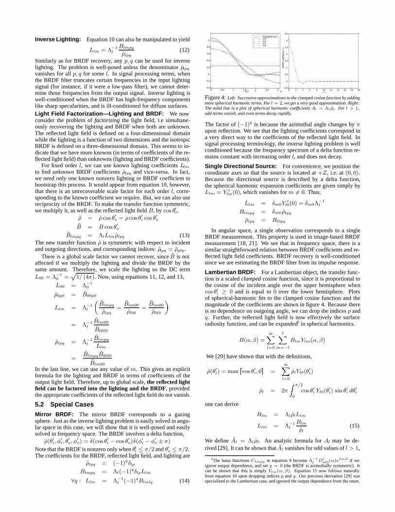
Figure 4: Left: Successive approximations to the clamped cosine function by addingmore spherical harmonic terms. For l = 2, we get a very good approximation. Right:The solid line is a plot of spherical harmonic coefficients Al = Λlρl. For l > 1,odd terms vanish, and even terms decay rapidly.

The factor of (−1)q is because the azimuthal angle changes by πupon reflection. We see that the lighting coefficients correspond ina very direct way to the coefficients of the reflected light field. Insignal processing terminology, the inverse lighting problem is wellconditioned because the frequency spectrum of a delta function re-mains constant with increasing order l, and does not decay.

Single Directional Source: For convenience, we position thecoordinate axes so that the source is located at +Z, i.e. at (0, 0).Because the directional source is described by a delta function,the spherical harmonic expansion coefficients are given simply byLlm = Y ∗

lm(0), which vanishes for m = 0. Thus,

Llm = δm0Y∗l0(0) = δm0Λ

−1l

Blmpq = δm0ρlpq

ρlpq = Bl0pq

In angular space, a single observation corresponds to a singleBRDF measurement. This property is used in image-based BRDFmeasurement [18, 21]. We see that in frequency space, there is asimilar straightforward relation between BRDF coefficients and re-flected light field coefficients. BRDF recovery is well-conditionedsince we are estimating the BRDF filter from its impulse response.

Lambertian BRDF: For a Lambertian object, the transfer func-tion is a scaled clamped cosine function, since it is proportional tothe cosine of the incident angle over the upper hemisphere whencos θ′i ≥ 0 and is equal to 0 over the lower hemisphere. Plotsof spherical-harmonic fits to the clamped cosine function and themagnitude of the coefficients are shown in figure 4. Because thereis no dependence on outgoing angle, we can drop the indices p andq. Further, the reflected light field is now effectively the surfaceradiosity function, and can be expanded3 in spherical harmonics.

B(α, β) =∞X

l=0

lXm=−l

BlmYlm(α, β)

We [29] have shown that with the definitions,

ρ(θ′i) = maxcos θ′i, 0

=

∞Xl=0

ρlYl0(θ′i)

ρl = 2π

Z π/2

0

cos θ′i Yl0(θ′i) sin θ′i dθ

′i

one can derive

Blm = ΛlρlLlm

Llm = Λ−1l

Blm

ρl(15)

We define Al = Λlρl. An analytic formula for Al may be de-rived [29]. It can be shown that Al vanishes for odd values of l > 1,

3The basis functions Clmpq in equation 9 become Λ−1l Dl

m0(α)eImβ if we

ignore output dependence, and set q = 0 (the BRDF is azimuthally symmetric). Itcan be shown that this is simply Ylm(α, β). Equation 15 now follows naturallyfrom equation 10 upon dropping indices p and q. Our previous derivation [29] wasspecialized to the Lambertian case, and ignored the output dependence from the onset.

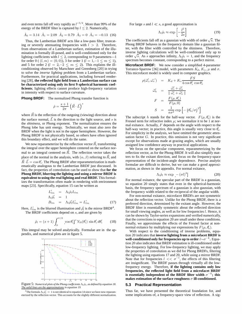
and even terms fall off very rapidly as l−5/2. More than 99% of theenergy of the BRDF filter is captured by l ≤ 2. Numerically,

A0 = 3.14 A1 = 2.09 A2 = 0.79 A3 = 0 A4 = −0.13 (16)

Thus, the Lambertian BRDF acts like a low-pass filter, truncat-ing or severely attenuating frequencies with l > 2. Therefore,from observations of a Lambertian surface, estimation of the illu-mination is formally ill-posed, and is well-conditioned only for thelighting coefficients with l ≤ 2, corresponding to 9 parameters—1for order 0 ( (l, m) = (0, 0)), 3 for order 1 (l = 1,−1 ≤ m ≤ 1),and 5 for order 2 (l = 2,−2 ≤ m ≤ 2). This explains the ill-conditioning observed by Marschner and Greenberg [20] in tryingto solve the inverse lighting problem from a Lambertian surface.Furthermore, for practical applications, including forward render-ing [28], the reflected light field from a Lambertian surface canbe characterized using only its first 9 spherical harmonic coef-ficients; lighting effects cannot produce high-frequency variationin intensity with respect to surface curvature.

Phong BRDF: The normalized Phong transfer function is

ρ =s + 1

2π

R · L

s

where R is the reflection of the outgoing (viewing) direction aboutthe surface normal, L is the direction to the light source, and s isthe shininess, or Phong exponent. The normalization ensures thePhong lobe has unit energy. Technically, we must also zero theBRDF when the light is not in the upper hemisphere. However, thePhong BRDF is not physically based, so others have often ignoredthis boundary effect, and we will do the same.

We now reparameterize by the reflection vector R, transformingthe integral over the upper hemisphere centered on the surface nor-mal to an integral centered on R. The reflection vector takes theplace of the normal in the analysis, with (α, β) referring to R, andR · L = cos θ′i. The Phong BRDF after reparameterization is math-ematically analogous to the Lambertian BRDF just discussed. Infact, the properties of convolution can be used to show that for thePhong BRDF, blurring the lighting and using a mirror BRDF isequivalent to using the real lighting and real BRDF. This formal-izes the transformation often made in rendering with environmentmaps [23]. Specifically, equation 15 can be written as

L′lm = ΛlρlLlm

Λlρ′l = 1

Blm = Λlρ′lL

′lm = L′

lm (17)

Here, L′lm is the blurred illumination and ρ′l is the mirror BRDF4.

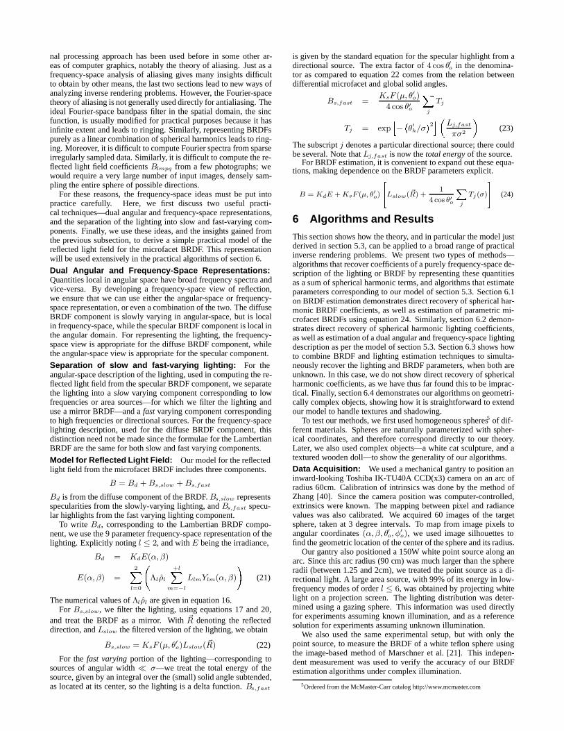
The BRDF coefficients depend on s, and are given by

ρl = (s + 1)

Z π/2

0

cos θ′i

sYl0(θ

′i) sin θ′i dθ

′i (18)

This integral may be solved analytically. Formulae are in the ap-pendix, and numerical plots are in figure 5.

0 2 4 6 8 10 12 14 16 18 20−0.2

0

0.2

0.4

0.6

0.8

1

1.2

l −>

BR

DF

coe

ffici

ent −

>

s=8 s=32 s=128 s=512

Figure 5: Numerical plots of the Phong coefficientsΛlρl , as defined by equation 18.The solid lines are the approximations in equation 19.

4The formulaΛlρ′l = 1 is not identical to equation 14 since we have now reparam-

eterized by the reflection vector. This accounts for the slightly different normalization.

For large s and l s, a good approximation is

Λlρl ≈ exp

− l2

2s

(19)

The coefficients fall off as a gaussian with width of order√s. The

Phong BRDF behaves in the frequency domain like a gaussian fil-ter, with the filter width controlled by the shininess. Therefore,inverse lighting calculations will be well-conditioned only up toorder

√s. As s approaches infinity, Λlρl = 1, and the frequency

spectrum becomes constant, corresponding to a perfect mirror.

Microfacet BRDF: We now consider a simplified 4-parameterTorrance-Sparrow [36] model, with parameters Kd, Ks, µ and σ.This microfacet model is widely used in computer graphics.

ρ(ω′i, ωo

′) = Kd + KsFS

4 cos θ′i cos θ′o

ω′h =

ω′i + ω′

o

‖ ω′i + ω′

o ‖

F =F (µ, θ′o)

F (µ, 0)

S =1

πσ2exp

h−θ′h/σ

2iThe subscript h stands for the half-way vector. F (µ, θ′o) is theFresnel term for refractive index µ; we normalize it to be 1 at nor-mal exitance. Actually, F depends on the angle with respect to thehalf-way vector; in practice, this angle is usually very close to θ′o.For simplicity in the analysis, we have omitted the geometric atten-uation factor G. In practice, this omission is not very significantexcept for observations made at grazing angles, which are usuallyassigned low confidence anyway in practical applications.

We focus on the specular component, reparameterizing by thereflection vector, as for the Phong BRDF. It will also simplify mat-ters to fix the exitant direction, and focus on the frequency-spacerepresentation of the incident-angle dependence. Precise analyticformulae are difficult to derive, but we can make a good approxi-mation, as shown in the appendix. For normal exitance,

Λlρl ≈ exp− (σl)2

(20)

For normal exitance, the specular part of the BRDF is a gaussian,so equation 20 simply states that even in the spherical-harmonicbasis, the frequency spectrum of a gaussian is also gaussian, withthe frequency width related to the reciprocal of the angular width.

For non-normal exitance, microfacet BRDFs are not symmetricabout the reflection vector. Unlike for the Phong BRDF, there is apreferred direction, determined by the exitant angle. However, theBRDF filter is essentially symmetric about the reflected directionfor small viewing angles, as well as for low frequencies l. Hence, itcan be shown by Taylor-series expansions and verified numerically,that the corrections to equation 20 are small under these conditions.Finally, we approximate the effects of the Fresnel factor at non-normal exitance by multiplying our expressions by F (µ, θ′o).

With respect to the conditioning of inverse problems, equa-tion 20 indicates that inverse lighting from a microfacet BRDF iswell-conditioned only for frequencies up to order l∼σ−1. Equa-tion 20 also indicates that BRDF estimation is ill-conditioned underlow-frequency lighting. For low-frequency lighting, we may applythe properties of convolution as we did for Phong BRDFs, filteringthe lighting using equations 17 and 20, while using a mirror BRDF.Note that for frequencies l << σ−1, the effects of this filteringare insignificant. The BRDF passes through virtually all the low-frequency energy. Therefore, if the lighting contains only lowfrequencies, the reflected light field from a microfacet BRDFis essentially independent of the BRDF filter width σ−1; thismakes estimation of the surface roughness σ ill-conditioned.

5.3 Practical Representation

Thus far, we have presented the theoretical foundation for, andsome implications of, a frequency-space view of reflection. A sig-

nal processing approach has been used before in some other ar-eas of computer graphics, notably the theory of aliasing. Just as afrequency-space analysis of aliasing gives many insights difficultto obtain by other means, the last two sections lead to new ways ofanalyzing inverse rendering problems. However, the Fourier-spacetheory of aliasing is not generally used directly for antialiasing. Theideal Fourier-space bandpass filter in the spatial domain, the sincfunction, is usually modified for practical purposes because it hasinfinite extent and leads to ringing. Similarly, representing BRDFspurely as a linear combination of spherical harmonics leads to ring-ing. Moreover, it is difficult to compute Fourier spectra from sparseirregularly sampled data. Similarly, it is difficult to compute the re-flected light field coefficients Blmpq from a few photographs; wewould require a very large number of input images, densely sam-pling the entire sphere of possible directions.

For these reasons, the frequency-space ideas must be put intopractice carefully. Here, we first discuss two useful practi-cal techniques—dual angular and frequency-space representations,and the separation of the lighting into slow and fast-varying com-ponents. Finally, we use these ideas, and the insights gained fromthe previous subsection, to derive a simple practical model of thereflected light field for the microfacet BRDF. This representationwill be used extensively in the practical algorithms of section 6.

Dual Angular and Frequency-Space Representations:Quantities local in angular space have broad frequency spectra andvice-versa. By developing a frequency-space view of reflection,we ensure that we can use either the angular-space or frequency-space representation, or even a combination of the two. The diffuseBRDF component is slowly varying in angular-space, but is localin frequency-space, while the specular BRDF component is local inthe angular domain. For representing the lighting, the frequency-space view is appropriate for the diffuse BRDF component, whilethe angular-space view is appropriate for the specular component.

Separation of slow and fast-varying lighting: For theangular-space description of the lighting, used in computing the re-flected light field from the specular BRDF component, we separatethe lighting into a slow varying component corresponding to lowfrequencies or area sources—for which we filter the lighting anduse a mirror BRDF—and a fast varying component correspondingto high frequencies or directional sources. For the frequency-spacelighting description, used for the diffuse BRDF component, thisdistinction need not be made since the formulae for the LambertianBRDF are the same for both slow and fast varying components.

Model for Reflected Light Field: Our model for the reflectedlight field from the microfacet BRDF includes three components.

B = Bd + Bs,slow + Bs,fast

Bd is from the diffuse component of the BRDF. Bs,slow representsspecularities from the slowly-varying lighting, and Bs,fast specu-lar highlights from the fast varying lighting component.

To write Bd, corresponding to the Lambertian BRDF compo-nent, we use the 9 parameter frequency-space representation of thelighting. Explicitly noting l ≤ 2, and with E being the irradiance,

Bd = KdE(α, β)

E(α, β) =2X

l=0

Λlρl

+lXm=−l

LlmYlm(α, β)

!(21)

The numerical values of Λlρl are given in equation 16.For Bs,slow, we filter the lighting, using equations 17 and 20,

and treat the BRDF as a mirror. With R denoting the reflecteddirection, and Lslow the filtered version of the lighting, we obtain

Bs,slow = KsF (µ, θ′o)Lslow(R) (22)

For the fast varying portion of the lighting—corresponding tosources of angular width σ—we treat the total energy of thesource, given by an integral over the (small) solid angle subtended,as located at its center, so the lighting is a delta function. Bs,fast

is given by the standard equation for the specular highlight from adirectional source. The extra factor of 4 cos θ′o in the denomina-tor as compared to equation 22 comes from the relation betweendifferential microfacet and global solid angles.

Bs,fast =KsF (µ, θ′o)

4 cos θ′o

Xj

Tj

Tj = exph−θ′h/σ

2iLj,fast

πσ2

(23)

The subscript j denotes a particular directional source; there couldbe several. Note that Lj,fast is now the total energy of the source.

For BRDF estimation, it is convenient to expand out these equa-tions, making dependence on the BRDF parameters explicit.

B = KdE + KsF (µ, θ′o)

24Lslow(R) +

1

4 cos θ′o

Xj

Tj(σ)

35 (24)

6 Algorithms and Results

This section shows how the theory, and in particular the model justderived in section 5.3, can be applied to a broad range of practicalinverse rendering problems. We present two types of methods—algorithms that recover coefficients of a purely frequency-space de-scription of the lighting or BRDF by representing these quantitiesas a sum of spherical harmonic terms, and algorithms that estimateparameters corresponding to our model of section 5.3. Section 6.1on BRDF estimation demonstrates direct recovery of spherical har-monic BRDF coefficients, as well as estimation of parametric mi-crofacet BRDFs using equation 24. Similarly, section 6.2 demon-strates direct recovery of spherical harmonic lighting coefficients,as well as estimation of a dual angular and frequency-space lightingdescription as per the model of section 5.3. Section 6.3 shows howto combine BRDF and lighting estimation techniques to simulta-neously recover the lighting and BRDF parameters, when both areunknown. In this case, we do not show direct recovery of sphericalharmonic coefficients, as we have thus far found this to be imprac-tical. Finally, section 6.4 demonstrates our algorithms on geometri-cally complex objects, showing how it is straightforward to extendour model to handle textures and shadowing.

To test our methods, we first used homogeneous spheres5 of dif-ferent materials. Spheres are naturally parameterized with spher-ical coordinates, and therefore correspond directly to our theory.Later, we also used complex objects—a white cat sculpture, and atextured wooden doll—to show the generality of our algorithms.

Data Acquisition: We used a mechanical gantry to position aninward-looking Toshiba IK-TU40A CCD(x3) camera on an arc ofradius 60cm. Calibration of intrinsics was done by the method ofZhang [40]. Since the camera position was computer-controlled,extrinsics were known. The mapping between pixel and radiancevalues was also calibrated. We acquired 60 images of the targetsphere, taken at 3 degree intervals. To map from image pixels toangular coordinates (α, β, θ′o, φ

′o), we used image silhouettes to

find the geometric location of the center of the sphere and its radius.Our gantry also positioned a 150W white point source along an

arc. Since this arc radius (90 cm) was much larger than the sphereradii (between 1.25 and 2cm), we treated the point source as a di-rectional light. A large area source, with 99% of its energy in low-frequency modes of order l ≤ 6, was obtained by projecting whitelight on a projection screen. The lighting distribution was deter-mined using a gazing sphere. This information was used directlyfor experiments assuming known illumination, and as a referencesolution for experiments assuming unknown illumination.

We also used the same experimental setup, but with only thepoint source, to measure the BRDF of a white teflon sphere usingthe image-based method of Marschner et al. [21]. This indepen-dent measurement was used to verify the accuracy of our BRDFestimation algorithms under complex illumination.

5Ordered from the McMaster-Carr catalog http://www.mcmaster.com

6.1 Inverse BRDF with Known Lighting

Estimation of Spherical Harmonic BRDF coefficients:Spherical harmonics and Zernike polynomials have been fit [14] tomeasured BRDF data, but previous work has not tried to estimatecoefficients directly. Since the BRDF is linear in the coefficientsρlpq, we simply solve a linear system to determine ρlpq.

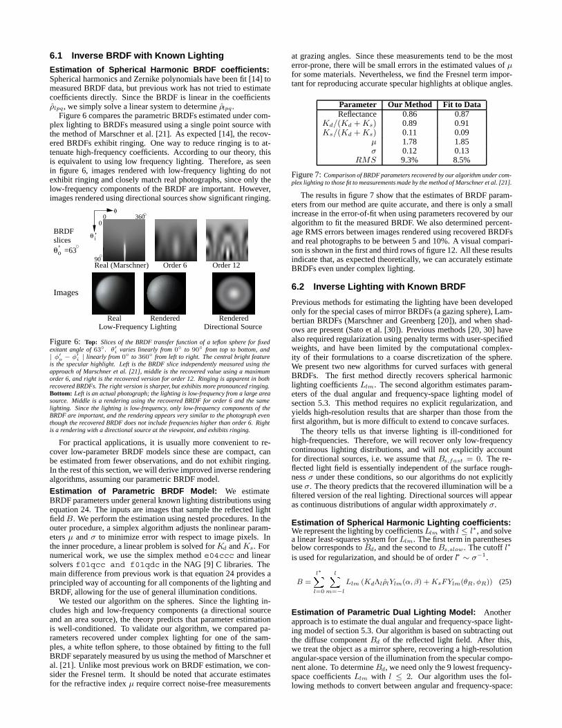
Figure 6 compares the parametric BRDFs estimated under com-plex lighting to BRDFs measured using a single point source withthe method of Marschner et al. [21]. As expected [14], the recov-ered BRDFs exhibit ringing. One way to reduce ringing is to at-tenuate high-frequency coefficients. According to our theory, thisis equivalent to using low frequency lighting. Therefore, as seenin figure 6, images rendered with low-frequency lighting do notexhibit ringing and closely match real photographs, since only thelow-frequency components of the BRDF are important. However,images rendered using directional sources show significant ringing.

Real (Marschner) Order 12Order 6

Images

i

φ

BRDFslices

Real

=63’oθ

RenderedLow-Frequency Lighting

RenderedDirectional Source

θ ’

00

360

90

Figure 6: Top: Slices of the BRDF transfer function of a teflon sphere for fixedexitant angle of 63. θ′i varies linearly from 0 to 90 from top to bottom, and| φ′

o − φ′i | linearly from 0 to 360 from left to right. The central bright feature

is the specular highlight. Left is the BRDF slice independently measured using theapproach of Marschner et al. [21], middle is the recovered value using a maximumorder 6, and right is the recovered version for order 12. Ringing is apparent in bothrecovered BRDFs. The right version is sharper, but exhibits more pronounced ringing.Bottom: Left is an actual photograph; the lighting is low-frequency from a large areasource. Middle is a rendering using the recovered BRDF for order 6 and the samelighting. Since the lighting is low-frequency, only low-frequency components of theBRDF are important, and the rendering appears very similar to the photograph eventhough the recovered BRDF does not include frequencies higher than order 6. Rightis a rendering with a directional source at the viewpoint, and exhibits ringing.

For practical applications, it is usually more convenient to re-cover low-parameter BRDF models since these are compact, canbe estimated from fewer observations, and do not exhibit ringing.In the rest of this section, we will derive improved inverse renderingalgorithms, assuming our parametric BRDF model.

Estimation of Parametric BRDF Model: We estimateBRDF parameters under general known lighting distributions usingequation 24. The inputs are images that sample the reflected lightfield B. We perform the estimation using nested procedures. In theouter procedure, a simplex algorithm adjusts the nonlinear param-eters µ and σ to minimize error with respect to image pixels. Inthe inner procedure, a linear problem is solved for Kd and Ks. Fornumerical work, we use the simplex method e04ccc and linearsolvers f01qcc and f01qdc in the NAG [9] C libraries. Themain difference from previous work is that equation 24 provides aprincipled way of accounting for all components of the lighting andBRDF, allowing for the use of general illumination conditions.

We tested our algorithm on the spheres. Since the lighting in-cludes high and low-frequency components (a directional sourceand an area source), the theory predicts that parameter estimationis well-conditioned. To validate our algorithm, we compared pa-rameters recovered under complex lighting for one of the sam-ples, a white teflon sphere, to those obtained by fitting to the fullBRDF separately measured by us using the method of Marschner etal. [21]. Unlike most previous work on BRDF estimation, we con-sider the Fresnel term. It should be noted that accurate estimatesfor the refractive index µ require correct noise-free measurements

at grazing angles. Since these measurements tend to be the mosterror-prone, there will be small errors in the estimated values of µfor some materials. Nevertheless, we find the Fresnel term impor-tant for reproducing accurate specular highlights at oblique angles.

Parameter Our Method Fit to DataReflectance 0.86 0.87

Kd/(Kd + Ks) 0.89 0.91Ks/(Kd + Ks) 0.11 0.09

µ 1.78 1.85σ 0.12 0.13

RMS 9.3% 8.5%

Figure 7: Comparison of BRDF parameters recovered by our algorithm under com-plex lighting to those fit to measurements made by the method of Marschner et al. [21].

The results in figure 7 show that the estimates of BRDF param-eters from our method are quite accurate, and there is only a smallincrease in the error-of-fit when using parameters recovered by ouralgorithm to fit the measured BRDF. We also determined percent-age RMS errors between images rendered using recovered BRDFsand real photographs to be between 5 and 10%. A visual compari-son is shown in the first and third rows of figure 12. All these resultsindicate that, as expected theoretically, we can accurately estimateBRDFs even under complex lighting.

6.2 Inverse Lighting with Known BRDF

Previous methods for estimating the lighting have been developedonly for the special cases of mirror BRDFs (a gazing sphere), Lam-bertian BRDFs (Marschner and Greenberg [20]), and when shad-ows are present (Sato et al. [30]). Previous methods [20, 30] havealso required regularization using penalty terms with user-specifiedweights, and have been limited by the computational complex-ity of their formulations to a coarse discretization of the sphere.We present two new algorithms for curved surfaces with generalBRDFs. The first method directly recovers spherical harmoniclighting coefficients Llm. The second algorithm estimates param-eters of the dual angular and frequency-space lighting model ofsection 5.3. This method requires no explicit regularization, andyields high-resolution results that are sharper than those from thefirst algorithm, but is more difficult to extend to concave surfaces.

The theory tells us that inverse lighting is ill-conditioned forhigh-frequencies. Therefore, we will recover only low-frequencycontinuous lighting distributions, and will not explicitly accountfor directional sources, i.e. we assume that Bs,fast = 0. The re-flected light field is essentially independent of the surface rough-ness σ under these conditions, so our algorithms do not explicitlyuse σ. The theory predicts that the recovered illumination will be afiltered version of the real lighting. Directional sources will appearas continuous distributions of angular width approximately σ.

Estimation of Spherical Harmonic Lighting coefficients:We represent the lighting by coefficients Llm with l ≤ l∗, and solvea linear least-squares system for Llm. The first term in parenthesesbelow corresponds to Bd, and the second to Bs,slow. The cutoff l∗

is used for regularization, and should be of order l∗ ∼ σ−1.

B =l∗X

l=0

lXm=−l

Llm (KdΛlρlYlm(α, β) + KsFYlm(θR, φR)) (25)

Estimation of Parametric Dual Lighting Model: Anotherapproach is to estimate the dual angular and frequency-space light-ing model of section 5.3. Our algorithm is based on subtracting outthe diffuse component Bd of the reflected light field. After this,we treat the object as a mirror sphere, recovering a high-resolutionangular-space version of the illumination from the specular compo-nent alone. To determine Bd, we need only the 9 lowest frequency-space coefficients Llm with l ≤ 2. Our algorithm uses the fol-lowing methods to convert between angular and frequency-space:

Phase 2

Phase 1Input

+

=

θ

φ

L

B

B

s,slowB

L

d1Bd

2

1lm lmL2

Figure 8: Estimation of dual lighting representation. In phase 1, we use frequency-space parametersL1

lm to compute diffuse componentB1d . This is subtracted from the

input image, leaving the specular component, from which the angular-space lightingis found. In phase 2, we compute coefficients L2

lm, which can be used to determineB2

d. The consistency condition is that B1d = B2

d or L1lm = L2

lm. In this and allsubsequent figures, the lighting is visualized by unwrapping the sphere so θ ranges inequal increments from 0 to π from top to bottom, and φ ranges in equal incrementsfrom 0 to 2π from left to right (so the image wraps around in the horizontal direction).

1. 9 parameters to High-Resolution Lighting: The inputs tophase 1 are the coefficients L1

lm. These suffice to find B1d by

equation 21. Since we assumed that Bs,fast = 0,

Bs,slow = KsF (µ, θ′o)Lslow(R) = B −B1d(L1

lm)

Lslow(R) =B −B1

d(L1lm)

KsF (µ, θ′o)

We assume the BRDF parameters are known, and B is theinput to the algorithm, so the right-hand side can be evaluated.

2. High-Resolution Lighting to 9 parameters: Using the an-gular space values L found from the first phase, we can easilyfind the 9 frequency-space parameters of the lighting L2

lm.

Now, assume we run phase 1 (with inputs L1lm) and phase 2

(with outputs L2lm) sequentially. The consistency condition is that

L1lm = L2

lm—converting from frequency to angular to frequencyspace must not change the result. Equivalently, the computed dif-fuse components must match, i.e. B1

d(L1lm) = B2

d(L2lm). This is

illustrated in figure 8. Since everything is linear in terms of thelighting coefficients, the consistency condition reduces to a systemof 9 simultaneous equations. After solving for Llm, we run phase1 to determine the high-resolution lighting in angular space.

Figure 9 compares the methods to each other, and to a refer-ence solution from a gazing sphere. Both algorithms give reason-ably accurate results. As predicted by the theory, high-frequencycomponents are filtered by the roughness σ. In the first method,involving direct recovery of Llm, there will still be some resid-ual energy for l > l∗. Since we regularize by not consideringhigher frequencies—we could increase l∗, but this makes the resultnoisier—the recovered lighting is somewhat blurred compared toour dual angular and frequency-space algorithm (second method).

*Real (Gazing Sphere) Algorithm 1 l = 12 *l = 20 Algorithm 2

φ

θ

Figure 9: Comparison of inverse lighting methods. From left to right, real lighting(from a gazing sphere), recovered illumination by direct estimation of spherical har-monic coefficients with l∗ = 12 and l∗ = 20, and estimation of dual angular andfrequency-space lighting model. To make the artifacts more apparent, we have set 0to gray. The results from the dual algorithm are sharper, but still somewhat blurredbecause of filtering by σ. A small amount of ringing occurs for direct coefficient re-covery, and can be seen for l∗ = 12. Using l∗ = 20 makes the solution very noisy.

6.3 Factorization—Unknown Lighting and BRDF

We can combine the inverse-BRDF and inverse-lighting methodsto factor the reflected light field, simultaneously recovering thelighting and BRDF when both are unknown. Therefore, we areable to recover BRDFs of curved surfaces under unknown complex

illumination, something which has not previously been demon-strated. There is an unrecoverable global scale factor, so we setKd + Ks = 1; we cannot find absolute reflectance. Also, thetheory predicts that for low-frequency lighting, estimation of thesurface roughness σ is ill-conditioned—blurring the lighting whilesharpening the BRDF does not significantly change the reflectedlight field. However, for high-frequency lighting, this ambiguitycan be removed. We will use a single manually specified direc-tional source in the recovered lighting distribution to estimate σ.

Algorithm: The algorithm consists of nested procedures. Inthe outer loop, we effectively solve an inverse-BRDF problem—anonlinear simplex algorithm adjusts the BRDF parameters tominimize error with respect to image pixels. Since Kd + Ks = 1,and σ will not be solved for till after the lighting and other BRDFparameters have been recovered, there are only 2 free parameters,Ks and µ. In the inner procedure, a linear problem is solved toestimate the lighting for a given set of BRDF parameters, using themethods of the previous subsection. Pseudocode is given below.

global Binput // Input imagesglobal Kd,Ks,µ,σ // BRDF parametersglobal L // Lightingprocedure Factor

Minimize(Ks,µ,ObjFun) // Simplex Methodσ = FindRoughness(L) // Figure 10, Equation 26

function ObjFun(Ks,µ)Kd = 1 −Ks // Kd + Ks = 1L = Lighting(Kd,Ks,µ) // Inverse LightingBpred = Predict(L,Kd,Ks,µ) // Predicted Light Fieldreturn RMS(Binput,Bpred) // RMS Error

Finding σ using a directional source: If a directionalsource is present—and manually specified by us in the recoveredlighting—we can estimate σ by equating specular components pre-dicted by equations 22 and 23 for the center, i.e. brightest point, ofthe light source at normal exitance. An illustration is in figure 10.

Lcen ≈ Ltotal

4πσ2(26)

= 0.14

θ

φ

tot

L cen = 1.0

σ = 0.11

L

Figure 10: We manually specify (red box) the region corresponding to the direc-tional source in a visualization of the lighting. The algorithm then determines Lcen,the intensity at the center (brightest point), Ltot, the total energy integrated over theregion specified by the red box, and computes σ using equation 26. The method doesnot depend on the size of the red box—provided it encloses the entire (filtered) source—nor the precise shape into which the source is filtered in the recovered lighting.

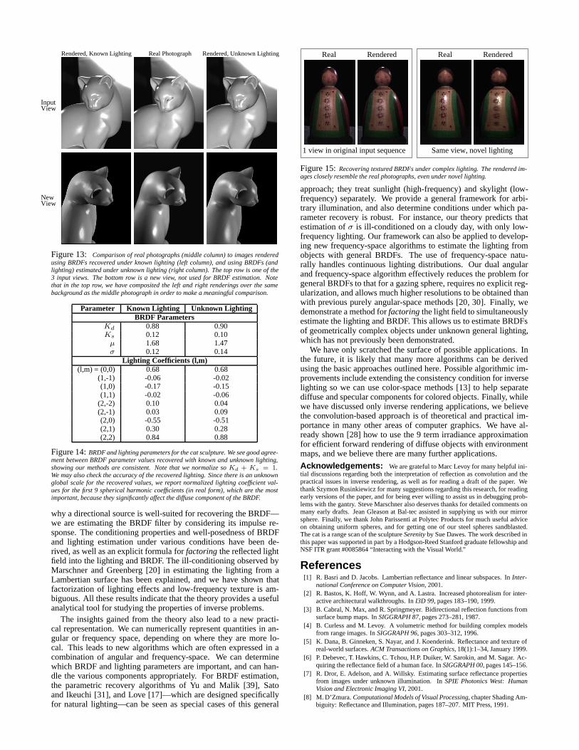
Results: We used the method of this subsection—with the dualangular and frequency-space algorithm for inverse lighting—to fac-tor the light field for the spheres, simultaneously estimating theBRDF and lighting. The same setup and lighting were used forall the spheres so we could compare the recovered illumination.

We see from figure 11 that the BRDF estimates under unknownlighting are accurate. Absolute errors are small, compared to pa-rameters recovered under known lighting. The only significantanomalies are the slightly low values for the refractive index µ—caused because we cannot know the high-frequency lighting com-ponents, which are necessary for more accurately estimating theFresnel term. We are also able to estimate a filtered version of thelighting. As shown in figure 12, the recovered lighting distribu-tions from all the samples are largely consistent. As predicted bythe theory, the directional source is spread out to different extentsdepending on how rough the surface is, i.e. the value of σ. Finally,figure 12 shows that rendered images using the estimated lightingand BRDF are almost indistinguishable from real photographs.

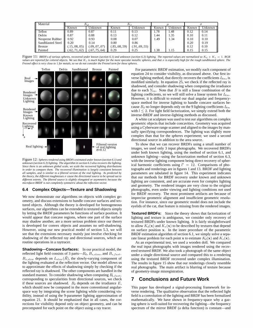
Material Kd Ks µ σKnown Unknown Known Unknown Known Unknown Known Unknown

Teflon 0.89 0.87 0.11 0.13 1.78 1.48 0.12 0.14Delrin 0.87 0.88 0.13 0.12 1.44 1.35 0.10 0.11Neoprene Rubber 0.92 0.93 0.08 0.07 1.49 1.34 0.10 0.10Sandblasted Steel 0.20 0.14 0.80 0.86 0.20 0.19Bronze (.15,.08,.05) (.09,.07,.07) (.85,.68,.59) (.91,.69,.55) 0.12 0.10Painted (.62,.71,.62) (.67,.75,.64) 0.29 0.25 1.38 1.15 0.15 0.15

Figure 11: BRDFs of various spheres, recovered under known (section 6.1) and unknown (section 6.3) lighting. The reported values are normalized soKd + Ks = 1. RGBvalues are reported for colored objects. We see thatKs is much higher for the more specular metallic spheres, and that σ is especially high for the rough sandblasted sphere. TheFresnel effect is very close to 1 for metals, so we do not consider the Fresnel term for these spheres.

LightingKnown

LightingUnknown

Lighting

Images

Images

Images

BronzeSandblasted PaintedDelrin

φ

Teflon

σ=0.12of real lightingFiltered version

θ

Real

Rendered

Rendered

Recovered

Real lighting

Figure 12: Spheres rendered using BRDFs estimated under known (section 6.1) andunknown (section 6.3) lighting. The algorithm in section 6.3 also recovers the lighting.Since there is an unknown global scale, we scale the recovered lighting distributionsin order to compare them. The recovered illumination is largely consistent betweenall samples, and is similar to a filtered version of the real lighting. As predicted bythe theory, the different roughnesses σ cause the directional source to be spread out todifferent extents. The filtered source is slightly elongated or asymmetric because themicrofacet BRDF is not completely symmetric about the reflection vector.

6.4 Complex Objects—Texture and Shadowing

We now demonstrate our algorithms on objects with complex ge-ometry, and discuss extensions to handle concave surfaces and tex-tured objects. Although the theory is developed for homogeneoussurfaces, our algorithms can be extended to textured objects simplyby letting the BRDF parameters be functions of surface position. Itwould appear that concave regions, where one part of the surfacemay shadow another, are a more serious problem since our theoryis developed for convex objects and assumes no self-shadowing.However, using our new practical model of section 5.3, we willsee that the extensions necessary mainly just involve checking forshadowing of the reflected ray and directional sources, which areroutine operations in a raytracer.

Shadowing—Concave Surfaces: In our practical model, thereflected light field consists of 3 parts—Bd, Bs,slow, and Bs,fast.Bs,slow depends on Lslow(R), the slowly-varying component ofthe lighting evaluated at the reflection vector. Our model allows usto approximate the effects of shadowing simply by checking if thereflected ray is shadowed. The other components are handled in thestandard manner. To consider shadowing when computing Bs,fast,corresponding to specularities from directional sources, we checkif these sources are shadowed. Bd depends on the irradiance E,which should now be computed in the more conventional angular-space way by integrating the scene lighting while considering vis-ibility, instead of using the 9-parameter lighting approximation ofequation 21. It should be emphasized that in all cases, the cor-rections for visibility depend only on object geometry, and can beprecomputed for each point on the object using a ray tracer.

For parametric BRDF estimation, we modify each component ofequation 24 to consider visibility, as discussed above. Our first in-verse lighting method, that directly recovers the coefficients Llm, ismodified similarly. In equation 25, we check if the reflected ray isshadowed, and consider shadowing when computing the irradiancedue to each Ylm. Note that B is still a linear combination of thelighting coefficients, so we will still solve a linear system for Llm.However, it is difficult to extend our dual angular and frequency-space method for inverse lighting to handle concave surfaces be-cause Bd no longer depends only on the 9 lighting coefficients Llm

with l ≤ 2. For light field factorization, we simply extend both theinverse-BRDF and inverse-lighting methods as discussed.

A white cat sculpture was used to test our algorithms on complexgeometric objects that include concavities. Geometry was acquiredusing a Cyberware range scanner and aligned to the images by man-ually specifying correspondences. The lighting was slightly morecomplex than that for the spheres experiment; we used a seconddirectional source in addition to the area source.

To show that we can recover BRDFs using a small number ofimages, we used only 3 input photographs. We recovered BRDFsunder both known lighting, using the method of section 6.1, andunknown lighting—using the factorization method of section 6.3,with the inverse lighting component being direct recovery of spher-ical harmonic coefficients using l∗ = 12. Comparisons of pho-tographs and renderings are in figures 1 and 13. BRDF and lightingparameters are tabulated in figure 14. This experiment indicatesthat our methods for BRDF recovery under known and unknownlighting are consistent, and are accurate even for complex lightingand geometry. The rendered images are very close to the originalphotographs, even under viewing and lighting conditions not usedfor BRDF recovery. The most prominent artifacts are because ofimprecise geometric alignment and insufficient geometric resolu-tion. For instance, since our geometric model does not include theeyelids of the cat, that feature is missing from the rendered images.

Textured BRDFs: Since the theory shows that factorization oflighting and texture is ambiguous, we consider only recovery oftextured BRDFs under known lighting. It is fairly straightforwardto allow Kd(x) and Ks(x) to be described by textures that dependon surface position x. In the inner procedure of the parametricBRDF estimation algorithm of section 6.1, we simply solve a sepa-rate linear problem for each point x to estimate Kd(x) and Ks(x).

As an experimental test, we used a wooden doll. We comparedthe real input photographs with images rendered using the recov-ered textured BRDF. We also took a photograph of the same objectunder a single directional source and compared this to a renderingusing the textured BRDF recovered under complex illumination.The results in figure 15 show that our renderings closely resemblereal photographs. The main artifact is blurring of texture becauseof geometry-image misregistration.

7 Conclusions and Future Work

This paper has developed a signal-processing framework for in-verse rendering. The qualitative observation that the reflected lightfield is a convolution of the lighting and BRDF has been formalizedmathematically. We have shown in frequency-space why a gaz-ing sphere is well-suited for recovering the lighting—the frequencyspectrum of the mirror BRDF (a delta function) is constant—and

InputView

NewView

Rendered, Known Lighting Real Photograph Rendered, Unknown Lighting

Figure 13: Comparison of real photographs (middle column) to images renderedusing BRDFs recovered under known lighting (left column), and using BRDFs (andlighting) estimated under unknown lighting (right column). The top row is one of the3 input views. The bottom row is a new view, not used for BRDF estimation. Notethat in the top row, we have composited the left and right renderings over the samebackground as the middle photograph in order to make a meaningful comparison.

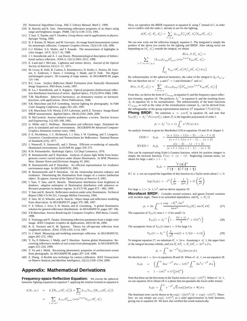
Parameter Known Lighting Unknown LightingBRDF Parameters

Kd 0.88 0.90Ks 0.12 0.10

µ 1.68 1.47σ 0.12 0.14

Lighting Coefficients (l,m)(l,m) = (0,0) 0.68 0.68

(1,-1) -0.06 -0.02(1,0) -0.17 -0.15(1,1) -0.02 -0.06

(2,-2) 0.10 0.04(2,-1) 0.03 0.09(2,0) -0.55 -0.51(2,1) 0.30 0.28(2,2) 0.84 0.88

Figure 14: BRDF and lighting parameters for the cat sculpture. We see good agree-ment between BRDF parameter values recovered with known and unknown lighting,showing our methods are consistent. Note that we normalize so Kd + Ks = 1.We may also check the accuracy of the recovered lighting. Since there is an unknownglobal scale for the recovered values, we report normalized lighting coefficient val-ues for the first 9 spherical harmonic coefficients (in real form), which are the mostimportant, because they significantly affect the diffuse component of the BRDF.

why a directional source is well-suited for recovering the BRDF—we are estimating the BRDF filter by considering its impulse re-sponse. The conditioning properties and well-posedness of BRDFand lighting estimation under various conditions have been de-rived, as well as an explicit formula for factoring the reflected lightfield into the lighting and BRDF. The ill-conditioning observed byMarschner and Greenberg [20] in estimating the lighting from aLambertian surface has been explained, and we have shown thatfactorization of lighting effects and low-frequency texture is am-biguous. All these results indicate that the theory provides a usefulanalytical tool for studying the properties of inverse problems.

The insights gained from the theory also lead to a new practi-cal representation. We can numerically represent quantities in an-gular or frequency space, depending on where they are more lo-cal. This leads to new algorithms which are often expressed in acombination of angular and frequency-space. We can determinewhich BRDF and lighting parameters are important, and can han-dle the various components appropriately. For BRDF estimation,the parametric recovery algorithms of Yu and Malik [39], Satoand Ikeuchi [31], and Love [17]—which are designed specificallyfor natural lighting—can be seen as special cases of this general

Rendered Real Rendered

1 view in original input sequence Same view, novel lighting

Real

Figure 15: Recovering textured BRDFs under complex lighting. The rendered im-ages closely resemble the real photographs, even under novel lighting.

approach; they treat sunlight (high-frequency) and skylight (low-frequency) separately. We provide a general framework for arbi-trary illumination, and also determine conditions under which pa-rameter recovery is robust. For instance, our theory predicts thatestimation of σ is ill-conditioned on a cloudy day, with only low-frequency lighting. Our framework can also be applied to develop-ing new frequency-space algorithms to estimate the lighting fromobjects with general BRDFs. The use of frequency-space natu-rally handles continuous lighting distributions. Our dual angularand frequency-space algorithm effectively reduces the problem forgeneral BRDFs to that for a gazing sphere, requires no explicit reg-ularization, and allows much higher resolutions to be obtained thanwith previous purely angular-space methods [20, 30]. Finally, wedemonstrate a method for factoring the light field to simultaneouslyestimate the lighting and BRDF. This allows us to estimate BRDFsof geometrically complex objects under unknown general lighting,which has not previously been demonstrated.

We have only scratched the surface of possible applications. Inthe future, it is likely that many more algorithms can be derivedusing the basic approaches outlined here. Possible algorithmic im-provements include extending the consistency condition for inverselighting so we can use color-space methods [13] to help separatediffuse and specular components for colored objects. Finally, whilewe have discussed only inverse rendering applications, we believethe convolution-based approach is of theoretical and practical im-portance in many other areas of computer graphics. We have al-ready shown [28] how to use the 9 term irradiance approximationfor efficient forward rendering of diffuse objects with environmentmaps, and we believe there are many further applications.

Acknowledgements: We are grateful to Marc Levoy for many helpful ini-tial discussions regarding both the interpretation of reflection as convolution and thepractical issues in inverse rendering, as well as for reading a draft of the paper. Wethank Szymon Rusinkiewicz for many suggestions regarding this research, for readingearly versions of the paper, and for being ever willing to assist us in debugging prob-lems with the gantry. Steve Marschner also deserves thanks for detailed comments onmany early drafts. Jean Gleason at Bal-tec assisted in supplying us with our mirrorsphere. Finally, we thank John Parissenti at Polytec Products for much useful adviceon obtaining uniform spheres, and for getting one of our steel spheres sandblasted.The cat is a range scan of the sculpture Serenity by Sue Dawes. The work described inthis paper was supported in part by a Hodgson-Reed Stanford graduate fellowship andNSF ITR grant #0085864 “Interacting with the Visual World.”

References[1] R. Basri and D. Jacobs. Lambertian reflectance and linear subspaces. In Inter-

national Conference on Computer Vision, 2001.[2] R. Bastos, K. Hoff, W. Wynn, and A. Lastra. Increased photorealism for inter-

active architectural walkthroughs. In I3D 99, pages 183–190, 1999.[3] B. Cabral, N. Max, and R. Springmeyer. Bidirectional reflection functions from

surface bump maps. In SIGGRAPH 87, pages 273–281, 1987.[4] B. Curless and M. Levoy. A volumetric method for building complex models

from range images. In SIGGRAPH 96, pages 303–312, 1996.[5] K. Dana, B. Ginneken, S. Nayar, and J. Koenderink. Reflectance and texture of

real-world surfaces. ACM Transactions on Graphics, 18(1):1–34, January 1999.[6] P. Debevec, T. Hawkins, C. Tchou, H.P. Duiker, W. Sarokin, and M. Sagar. Ac-

quiring the reflectance field of a human face. In SIGGRAPH 00, pages 145–156.[7] R. Dror, E. Adelson, and A. Willsky. Estimating surface reflectance properties

from images under unknown illumination. In SPIE Photonics West: HumanVision and Electronic Imaging VI, 2001.

[8] M. D’Zmura. Computational Models of Visual Processing, chapter Shading Am-biguity: Reflectance and Illumination, pages 187–207. MIT Press, 1991.

[9] Numerical Algorithms Group. NAG C Library Manual, Mark 5. 1999.[10] K. Ikeuchi and K. Sato. Determining reflectance properties of an object using

range and brightness images. PAMI, 13(11):1139–1153, 1991.[11] T. Inui, Y. Tanabe, and Y. Onodera. Group theory and its applications in physics.

Springer Verlag, 1990.[12] K. F. Karner, H. Mayer, and M. Gervautz. An image based measurement system

for anisotropic reflection. Computer Graphics Forum, 15(3):119–128, 1996.[13] G.J. Klinker, S.A. Shafer, and T. Kanade. The measurement of highlights in

color images. IJCV, 2(1):7–32, 1988.[14] J. J. Koenderink and A. J. van Doorn. Phenomenological description of bidirec-

tional surface reflection. JOSA A, 15(11):2903–2912, 1998.[15] E. Land and J. McCann. Lightness and retinex theory. Journal of the Optical

Society of America, 61(1):1–11, 1971.[16] M. Levoy, K. Pulli, B. Curless, S. Rusinkiewicz, D. Koller, L. Pereira, M. Ginz-

ton, S. Anderson, J. Davis, J. Ginsberg, J. Shade, and D. Fulk. The digitalmichelangelo project: 3D scanning of large statues. In SIGGRAPH 00, pages131–144.

[17] R.C. Love. Surface Reflection Model Estimation from Naturally IlluminatedImage Sequences. PhD thesis, Leeds, 1997.

[18] R. Lu, J. Koenderink, and A. Kappers. Optical properties (bidirectional reflec-tion distribution functions) of velvet. Applied Optics, 37(25):5974–5984, 1998.

[19] T.M. MacRobert. Spherical harmonics; an elementary treatise on harmonicfunctions, with applications. Dover Publications, 1948.

[20] S.R. Marschner and D.P. Greenberg. Inverse lighting for photography. In FifthColor Imaging Conference, pages 262–265, 1997.

[21] S.R. Marschner, S.H. Westin, E.P.F. Lafortune, and K.E. Torrance. Image-BasedBRDF measurement. Applied Optics, 39(16):2592–2600, 2000.

[22] N. McCormick. Inverse radiative transfer problems: a review. Nuclear Scienceand Engineering, 112:185–198, 1992.

[23] G. Miller and C. Hoffman. Illumination and reflection maps: Simulated ob-jects in simulated and real environments. SIGGRAPH 84 Advanced ComputerGraphics Animation seminar notes, 1984.

[24] F. E. Nicodemus, J. C. Richmond, J. J. Hsia, I. W. Ginsberg, and T. Limperis.Geometric Considerations and Nomenclature for Reflectance. National Bureauof Standards (US), 1977.

[25] J. Nimeroff, E. Simoncelli, and J. Dorsey. Efficient re-rendering of naturallyilluminated environments. In EGWR 94, pages 359–373.

[26] R.W. Preisendorfer. Hydrologic Optics. US Dept Commerce, 1976.[27] R. Ramamoorthi and P. Hanrahan. Analysis of planar light fields from homo-

geneous convex curved surfaces under distant illumination. In SPIE PhotonicsWest: Human Vision and Electronic Imaging VI, 2001.

[28] R. Ramamoorthi and P. Hanrahan. An efficient representation for irradianceenvironment maps. In SIGGRAPH 01, 2001.

[29] R. Ramamoorthi and P. Hanrahan. On the relationship between radiance andirradiance: Determining the illumination from images of a convex lambertianobject. To appear, Journal of the Optical Society of America A, 2001.

[30] I. Sato, Y. Sato, and K. Ikeuchi. Illumination distribution from brightness inshadows: adaptive estimation of illumination distribution with unknown re-flectance properties in shadow regions. In ICCV 99, pages 875 – 882, 1999.

[31] Y. Sato and K. Ikeuchi. Reflectance analysis under solar illumination. TechnicalReport CMU-CS-94-221, Carnegie Mellon University, 1994.

[32] Y. Sato, M. D. Wheeler, and K. Ikeuchi. Object shape and reflectance modelingfrom observation. In SIGGRAPH 97, pages 379–388, 1997.

[33] F. X. Sillion, J. Arvo, S. H. Westin, and D. Greenberg. A global illuminationsolution for general reflectance distributions. In SIGGRAPH 91, pages 187–196.

[34] S.R.Marschner. Inverse Rendering for Computer Graphics. PhD thesis, Cornell,1998.

[35] S. Tominaga and N. Tanaka. Estimating reflection parameters from a single colorimage. IEEE Computer Graphics & Applications, 20(5):58–66, 2000.

[36] K. E. Torrance and E. M. Sparrow. Theory for off-specular reflection fromroughened surfaces. JOSA, 57(9):1105–1114, 1967.

[37] G. J. Ward. Measuring and modeling anisotropic reflection. In SIGGRAPH 92,pages 265–272, 1992.

[38] Y. Yu, P. Debevec, J. Malik, and T. Hawkins. Inverse global illumination: Re-covering reflectance models of real scenes from photographs. In SIGGRAPH 99,pages 215–224, 1999.

[39] Y. Yu and J. Malik. Recovering photometric properties of architectural scenesfrom photographs. In SIGGRAPH 98, pages 207–218, 1998.

[40] Z. Zhang. A flexible new technique for camera calibration. IEEE Transactionson Pattern Analysis and Machine Intelligence, 22(11):1330–1334, 2000.

Appendix: Mathematical Derivations

Frequency-space Reflection Equation: We rewrite the sphericalharmonic lighting expansion in equation 7, applying the rotation formula in equation 6.

L(θi, φi) = LRα,β(θ

′i, φ

′i)=Xl,m

LlmYlm

Rα,β(θ

′i, φ

′i)

=X

l,m,m′LlmD

lmm′ (α)e

ImβYlm′(θ′i, φ

′i)

Next, we reproduce the BRDF expansion in equation 8, using l′ instead of l, in ordernot to conflict with the index l, already in use for the lighting.

ρ(θ′i, φ′i, θ

′o, φ

′o) =

Xl′,p,q

ρl′pqY∗

l′q(θ′i, φ

′i)Ypq(θ

′o, φ

′o)

We can now write out the reflection integral, equation 5. The integrand is simply theproduct of the above two results for the lighting and BRDF. After taking terms notdepending on (θ′i, φ

′i) outside the integral, we obtain

B(α, β, θ′o, φ′o) =X

l,l′,m,m′,p,q

[Llmρl′pqDlmm′ (α)e

ImβYpq(θ′o, φ

′o) ·

ZΩ′

i

Ylm′(θ′i, φ

′i)Y

∗l′q(θ

′i, φ

′i) dω

′i]

By orthonormality of the spherical harmonics, the value of the integral is δll′δm′q .We can therefore setm′ = q and l′ = l and eliminate l′ andm′.

B(α, β, θ′o, φ′o) =

Xl,m,p,q

(Llmρlpq)Dl

mq(α)eImβYpq(θ

′o, φ

′o)

From this, we derive the form ofClmpq in equation 9, and the frequency-space reflec-tion formula, equation 10. The prefactor Λ−1

l in equation 9, and the resulting factorΛl in equation 10, is for normalization. The orthonormality of the basis functionsClmpq , as well as the value of the normalization constant Λl , can be derived fromthe orthogonality of the group representation matricesDl (equation 7.73 of [11]).

Phong BRDF: We substitute u = cos θ′i in equation 18, and note thatYl0(θ

′i) = Λ−1

l Pl(cos θ′i), where Pl is the legendre polynomial of order l.

ρl = Λ−1l (s+ 1)

Z 1

0usPl(u) d u

An analytic formula is given by MacRobert [19] in equations 19 and 20 of chapter 5.

ODD l Λlρl =(s+ 1)(s− 1)(s− 3) . . . (s− l+ 2)

(s + l+ 1)(s + l− 1) . . . (s+ 2)

EVEN l Λlρl =s(s− 2) . . . (s− l + 2)

(s+ l + 1)(s+ l − 1) . . . (s + 3)

This can be expressed using Euler’s Gamma function, which for positive integers issimply the factorial function, Γ(n) = (n − 1)!. Neglecting constant terms, weobtain for large s and s > l− 1,

Λlρl =

Γ

s2

2Γ

s2 − l

2

Γ

s2 + l

2

If l s, we can expand the logarithm of this function in a Taylor series about l = 0.

log(Λlρl) = −l2

1

2s−

1

2s2

+O

l4

s2

!

For large s, 1/s 1/s2, and we derive equation 19.

Microfacet BRDF: Consider normal exitance, and ignore Fresnel variationwith incident angle. There is no azimuthal dependence, and θ′h = θ′i/2.

ρl = 2π

Z π/2

0

exph−θ′i

2/4σ2i

4πσ2Yl0(θ

′i) sin θ

′i d θ

′i (27)

The expansion of Yl0(t) near t = 0 for small l is

Yl0(t) = Λ−1l

1−

l(l + 1)

4t2 + O(t4)

(28)

The asymptotic form of Yl0(t) near t = 0 for large l is

Yl0(t) ∼ Λ−1l

1√tcos[(l+ 1/2)t− π/4]

(29)

To integrate equation 27, we substitute θ′i = 2σu. Assuming σ 1, the upper limitof the integral becomes infinite, and sin θ′i d θ

′i = θ

′i d θ

′i = 4σ2u du.

ρl =

Z ∞

02e−u2

Yl0(2σu)u du

We therefore set t = 2σu in equations 28 and 29. Whenσl 1, we use equation 28.

Λlρl =

Z ∞

02ue−u2

d u− (σl)2Z ∞

02u3e−u2

d u

= 1− (σl)2+O

[σl]

4

Note that these are the first terms in the Taylor series of exp[−(σl)2]. Whenσl 1,we use equation 29 to obtain (Φ is a phase that encapsulates the lower-order terms):

Λlρl ∼Z ∞

0e−u2√

u cos[(2σl)u + Φ] d u

The dominant term can be shown to be exp[−(2σl)2/4] = exp[−(σl)2]. There-fore, we can simply use exp[−(σl)2] as a valid approximation in both domains,giving rise to equation 20. We have also verified this result numerically.