Embed Size (px)
Citation preview

Support Vector Machines
Mario Martin
CS-UPC
December 8, 2019
08/12/2019Mario Martin (CS-UPC) Support Vector Machines - DM

08/12/2019Mario Martin (CS-UPC) Support Vector Machines - DM
Outline
Large-margin linear classifierLinear separableNonlinear separable
Creating nonlinear classifiers: kernel trickDiscussion on SVMConclusion

SVM: Large-margin linear classifier
08/12/201908/12/2019Mario Martin (CS-UPC) 08/12/2019Mario Martin (CS-UPC) Support Vector Machines - DM

Binary classification can be viewed as the task of separating classes in feature space:
wTx + b = 0
wTx + b < 0wTx + b > 0
f(x) = sign(wTx + b)
Perceptron Revisited: Linear Separators
08/12/201908/12/2019Mario Martin (CS-UPC) 08/12/2019Mario Martin (CS-UPC) Support Vector Machines - DM

There are infinite linear separators. Are all them equally good?
08/12/201908/12/2019Mario Martin (CS-UPC) 08/12/2019Mario Martin (CS-UPC) Support Vector Machines - DM
Perceptron Revisited: Linear Separators

What is a good Decision Boundary?
Consider a two-class, linearly separable classification problem
Many decision boundaries! The Perceptron algorithm can be
used to find such a boundaryDifferent algorithms have been
proposed Are all decision boundaries
equally good? Class 1
Class 2
08/12/201908/12/2019Mario Martin (CS-UPC) 08/12/2019Mario Martin (CS-UPC) Support Vector Machines - DM
Examples of Bad Decision Boundaries
Class 1
Class 2
Class 1
Class 2
08/12/201908/12/2019Mario Martin (CS-UPC) 08/12/2019Mario Martin (CS-UPC) Support Vector Machines - DM
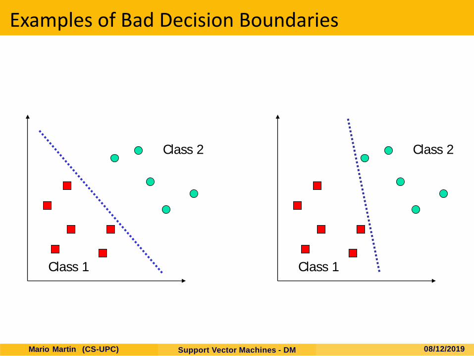
Examples of Bad Decision Boundaries
Class 1
Class 2
Class 1
Class 2
08/12/201908/12/2019Mario Martin (CS-UPC) 08/12/2019Mario Martin (CS-UPC) Support Vector Machines - DM
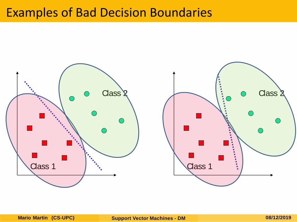
Better Decision Boundary
Class 1
Class 2
08/12/201908/12/2019Mario Martin (CS-UPC) 08/12/2019Mario Martin (CS-UPC) Support Vector Machines - DM

Better Decision Boundary
08/12/201908/12/2019Mario Martin (CS-UPC) 08/12/2019Mario Martin (CS-UPC) Support Vector Machines - DM
Class 1
Class 2

Decision Boundaries
08/12/201908/12/2019Mario Martin (CS-UPC) 08/12/2019Mario Martin (CS-UPC) Support Vector Machines - DM
Class 1
Class 2
Class 1
Class 2
Class 1
Class 2

• Distance from example xi to the separator is • Examples closest to the hyperplane are support vectors. • Margin ρ of the separator is the distance between support
vectors.
Classification Margin
wxw br i
T +=
r
ρ
08/12/201908/12/2019Mario Martin (CS-UPC) 08/12/2019Mario Martin (CS-UPC) Support Vector Machines - DM

Large-margin Decision Boundary
• The decision boundary should be as far away from the data of both classes as possible
• We should maximize the margin, m• Distance between the origin and the line wtx=k is k/||w||
Class 1
Class 2
m
08/12/201908/12/2019Mario Martin (CS-UPC) 08/12/2019Mario Martin (CS-UPC) Support Vector Machines - DM
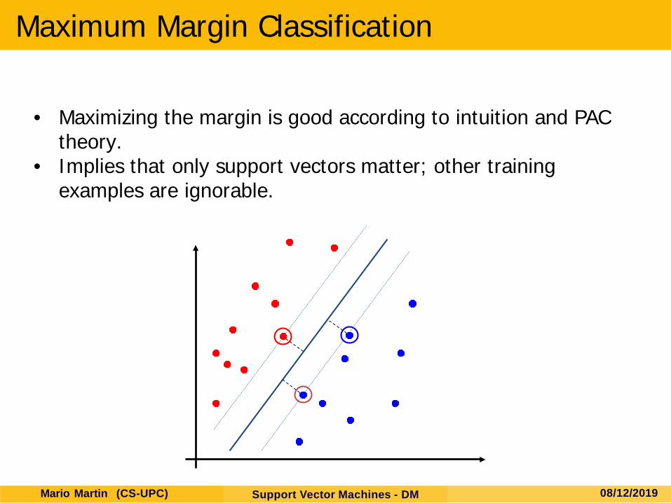
Maximum Margin Classification
• Maximizing the margin is good according to intuition and PAC theory.
• Implies that only support vectors matter; other training examples are ignorable.
08/12/201908/12/2019Mario Martin (CS-UPC) 08/12/2019Mario Martin (CS-UPC) Support Vector Machines - DM

Finding the Decision Boundary
08/12/201908/12/2019Mario Martin (CS-UPC) 08/12/2019Mario Martin (CS-UPC) Support Vector Machines - DM
Let {x1, ..., xn} be our data set and let yi ∈ {1,-1} be the class label of xi
The decision boundary should classify all points correctly
The decision boundary can be found by solving the following constrained optimization problem
This is a constrained optimization problem. Solving it requires some new tools Feel free to ignore the following several slides; what is important
is the constrained optimization problem above

Suppose we want to: minimize f(x) subject to g(x) = 0A necessary condition for x0 to be a solution:
α: the Lagrange multiplierFor multiple constraints gi(x) = 0, i=1, …, m, we need a
Lagrange multiplier αi for each of the constraints
[Recap of Constrained Optimization]
08/12/201908/12/2019Mario Martin (CS-UPC) 08/12/2019Mario Martin (CS-UPC) Support Vector Machines - DM
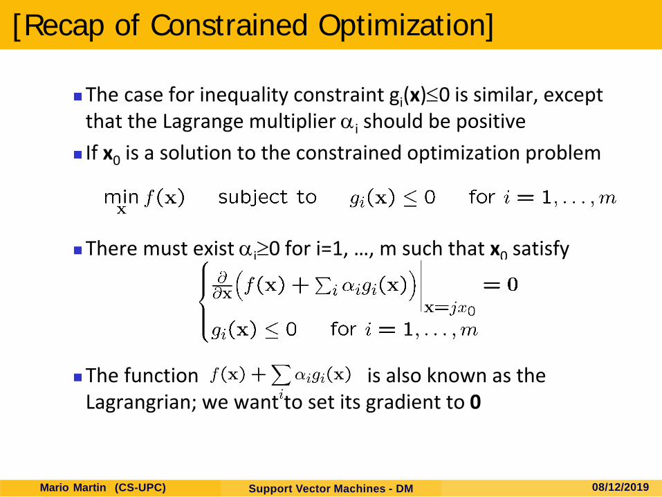
The case for inequality constraint gi(x)≤0 is similar, except that the Lagrange multiplier αi should be positive
If x0 is a solution to the constrained optimization problem
There must exist αi≥0 for i=1, …, m such that x0 satisfy
The function is also known as the Lagrangrian; we want to set its gradient to 0
[Recap of Constrained Optimization]
08/12/201908/12/2019Mario Martin (CS-UPC) 08/12/2019Mario Martin (CS-UPC) Support Vector Machines - DM

The Lagrangian is
Note that ||w||2 = wTw Setting the gradient of w.r.t. w and b to zero, we have
[Back to the Original Problem]
08/12/201908/12/201908/12/2019Mario Martin (CS-UPC) Support Vector Machines - DM

If we substitute to , we have
Note that
This is a function of αi only
[The Dual problem]
08/12/201908/12/201908/12/201908/12/201908/12/201908/12/2019Mario Martin (CS-UPC) Support Vector Machines - DM
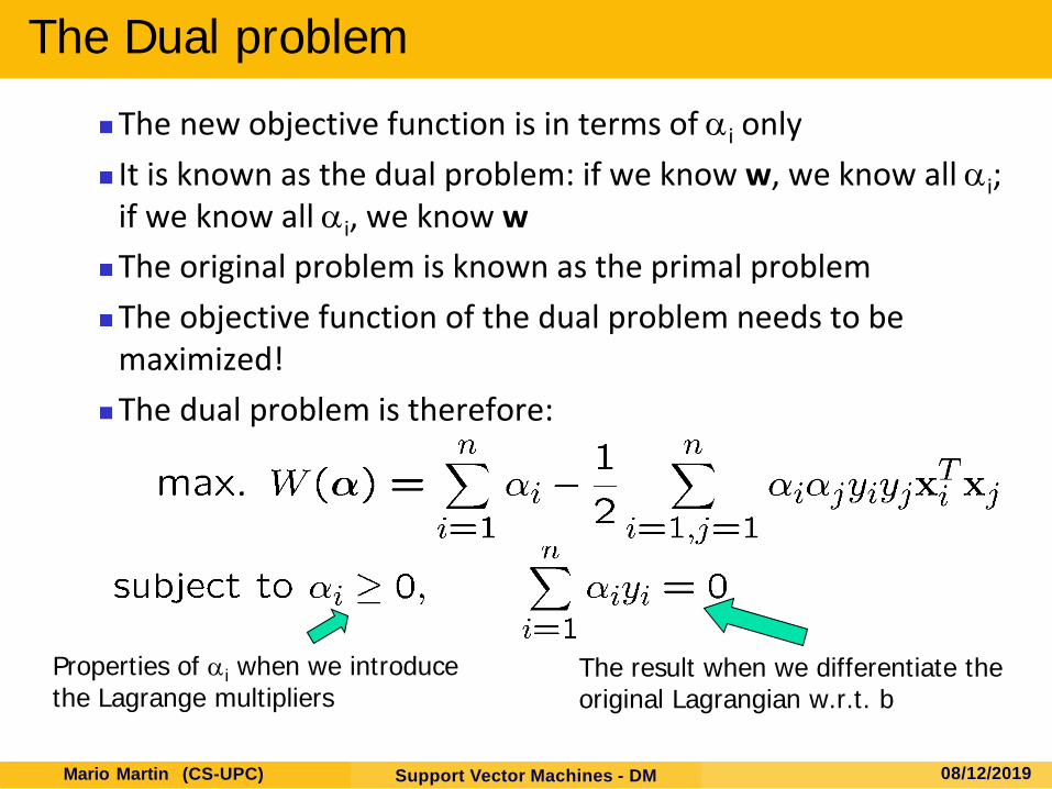
The new objective function is in terms of αi only It is known as the dual problem: if we know w, we know all αi;
if we know all αi, we know wThe original problem is known as the primal problemThe objective function of the dual problem needs to be
maximized!The dual problem is therefore:
Properties of αi when we introduce the Lagrange multipliers
The result when we differentiate the original Lagrangian w.r.t. b
The Dual problem
08/12/201908/12/201908/12/201908/12/201908/12/201908/12/2019Mario Martin (CS-UPC) Support Vector Machines - DM

This is a quadratic programming (QP) problem A global maximum of αi can always be found
w can be recovered by
The Dual problem
08/12/201908/12/201908/12/2019Mario Martin (CS-UPC) Support Vector Machines - DM

α6=1.4
Class 1
Class 2
α1=0.8
α2=0
α3=0
α4=0
α5=0α7=0
α8=0.6
α9=0
α10=0
A Geometrical interpretation
08/12/201908/12/201908/12/2019Mario Martin (CS-UPC) Support Vector Machines - DM

Many of the αi are zerow is a linear combination of a small number of data points This “sparse” representation can be viewed as data compression
as in the construction of knn classifier xi with non-zero αi are called support vectors (SV)
The decision boundary is determined only by the SV Let tj (j=1, ..., s) be the indices of the s support vectors. We can
writeFor testing with a new data z
Compute and classify z as class 1 if the sum is positive, and class 2 otherwise
Note: w need not be formed explicitly
Characteristics of the Solution
08/12/201908/12/201908/12/2019Mario Martin (CS-UPC) Support Vector Machines - DM

Many approaches have been proposed Loqo, cplex, etc. (see http://www.numerical.rl.ac.uk/qp/qp.html)
Most are “interior-point” methods Start with an initial solution that can violate the constraints Improve this solution by optimizing the objective function and/or
reducing the amount of constraint violationFor SVM, sequential minimal optimization (SMO) seems to be
the most popular A QP with two variables is trivial to solve Each iteration of SMO picks a pair of (αi,αj) and solve the QP with
these two variables; repeat until convergence In practice, we can just regard the QP solver as a “black-box”
without bothering how it works
The Quadratic Programming Problem
08/12/201908/12/201908/12/2019Mario Martin (CS-UPC) Support Vector Machines - DM

Non-linear separable datasets:Soft-Margin SVM
08/12/201908/12/2019Mario Martin (CS-UPC) 08/12/2019Mario Martin (CS-UPC) Support Vector Machines - DM

• Sometimes, data sets are not linearly separable.
Non-Separable Sets
08/12/201908/12/2019Mario Martin (CS-UPC) 08/12/2019Mario Martin (CS-UPC) Support Vector Machines - DM

• Sometimes, we do not want to separate perfectly.
This is too close!
Maybe this point is notso important.
Non-Separable Sets
08/12/201908/12/2019Mario Martin (CS-UPC) 08/12/2019Mario Martin (CS-UPC) Support Vector Machines - DM

• Sometimes, we do not want to separate perfectly.
Non-Separable Sets
The hyperplane is nicer!
If we ignorethis point
08/12/201908/12/2019Mario Martin (CS-UPC) 08/12/2019Mario Martin (CS-UPC) Support Vector Machines - DM

ξiξi
Slack variables ξi can be added to allow misclassification of difficult or noisy examples, resulting margin called soft.
Soft Margin Classification
08/12/201908/12/2019Mario Martin (CS-UPC) 08/12/2019Mario Martin (CS-UPC) Support Vector Machines - DM

We allow “error” ξi in classification; it is based on the output of the discriminant function wTx+b
ξi different from 0 for misclassified samples
Class 1
Class 2
Soft Margin Classification
08/12/201908/12/2019Mario Martin (CS-UPC) 08/12/2019Mario Martin (CS-UPC) Support Vector Machines - DM
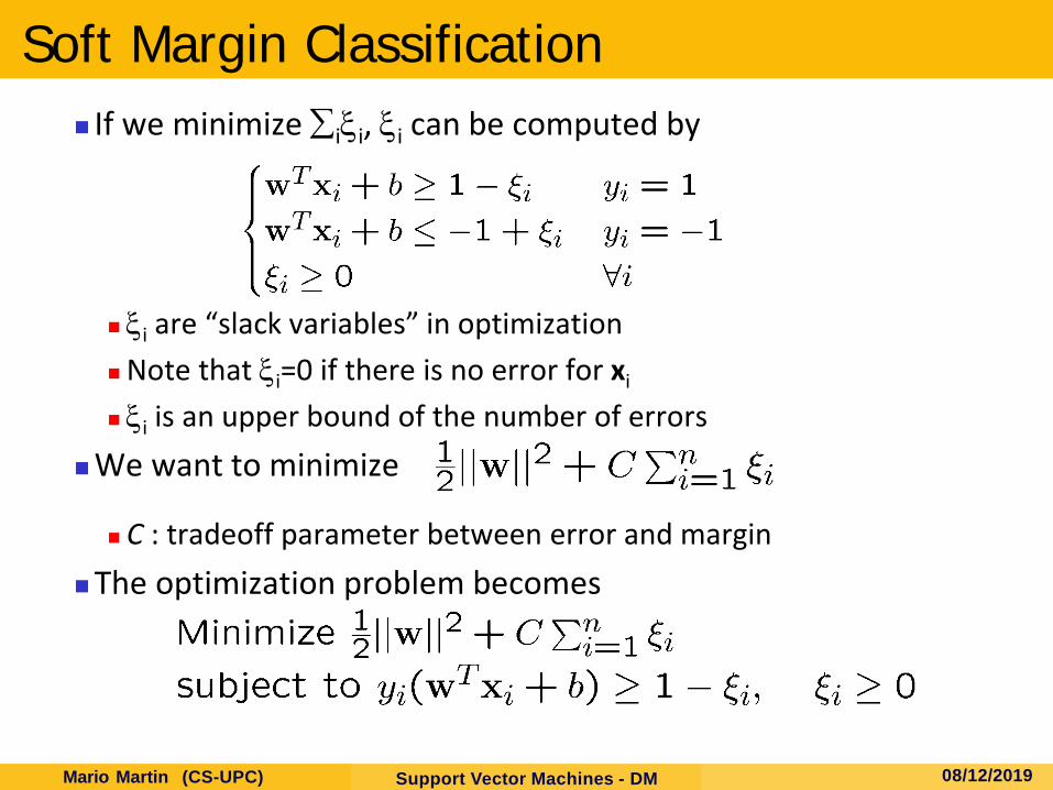
If we minimize ∑iξi, ξi can be computed by
ξi are “slack variables” in optimizationNote that ξi=0 if there is no error for xi
ξi is an upper bound of the number of errorsWe want to minimize
C : tradeoff parameter between error and marginThe optimization problem becomes
Soft Margin Classification
08/12/201908/12/2019Mario Martin (CS-UPC) 08/12/2019Mario Martin (CS-UPC) Support Vector Machines - DM
08/12/201908/12/2019Mario Martin (CS-UPC) 08/12/2019Mario Martin (CS-UPC) Support Vector Machines - DM
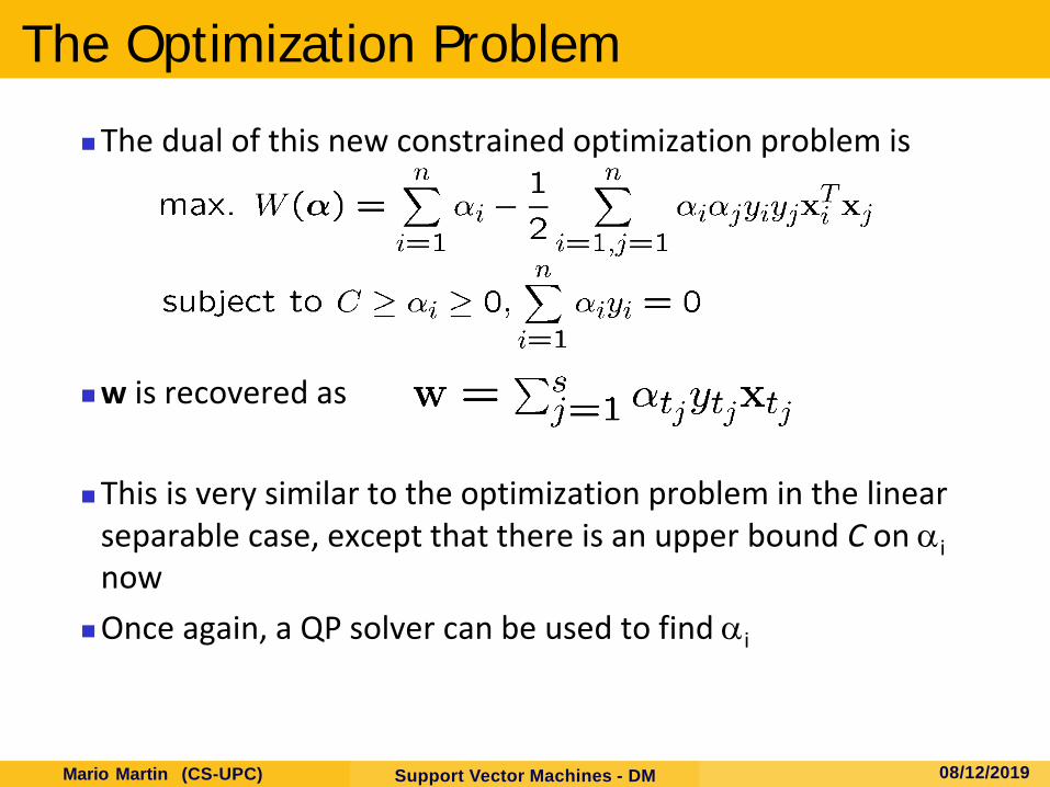
The dual of this new constrained optimization problem is
w is recovered as
This is very similar to the optimization problem in the linear separable case, except that there is an upper bound C on αi now
Once again, a QP solver can be used to find αi
The Optimization Problem

α6=1.0
Class 1
Class 2
α1=0.9
α2=0
α3=0.2
α4=0
α5=0.3α7=0
α8=0.6
α9=0
α10=0
A Geometrical interpretation
08/12/201908/12/201908/12/2019Mario Martin (CS-UPC) Support Vector Machines - DM
C = 1.0
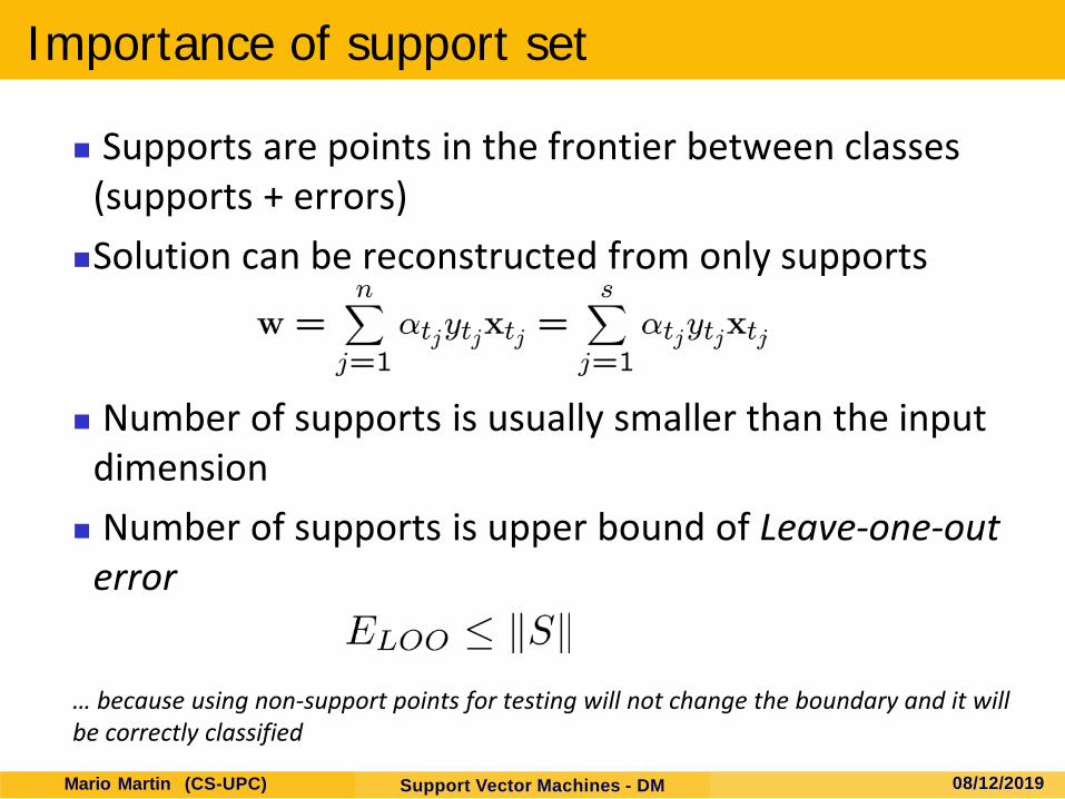
Supports are points in the frontier between classes (supports + errors) Solution can be reconstructed from only supports
Number of supports is usually smaller than the input dimension Number of supports is upper bound of Leave-one-out
error
… because using non-support points for testing will not change the boundary and it will be correctly classified
Importance of support set
08/12/201908/12/201908/12/2019Mario Martin (CS-UPC) Support Vector Machines - DM

Non-linear separable datasets:Kernel methods
08/12/201908/12/2019Mario Martin (CS-UPC) 08/12/2019Mario Martin (CS-UPC) Support Vector Machines - DM

08/12/201908/12/2019Mario Martin (CS-UPC) 08/12/2019Mario Martin (CS-UPC) Support Vector Machines - DM
Extension to Non-linear Decision BoundarySo far, we have only considered large-margin classifier with a
linear decision boundaryHow to generalize it to become nonlinear?Key idea: transform xi to a higher dimensional space to “make
life easier” Input space: the space the point xi are located Feature space: the space of φ(xi) after transformation
Why transform? Linear operation in the feature space is equivalent to non-linear
operation in input space Classification can become easier with a proper transformation. In
the XOR problem, for example, adding a new feature of x1x2make the problem linearly separable

General idea: the original feature space can be mapped to some higher-dimensional feature space where the training set is separable:
08/12/201908/12/2019Mario Martin (CS-UPC) 08/12/2019Mario Martin (CS-UPC) Support Vector Machines - DM
Moving data to higher dimensional space
φ( )
φ( )
φ( )φ( )φ( )
φ( )
φ( )φ( )
φ(.) φ( )
φ( )
φ( )φ( )φ( )
φ( )
φ( )
φ( )φ( ) φ( )
Feature spaceInput spaceNote: feature space is of higher dimension than the input space in practice

08/12/201908/12/2019Mario Martin (CS-UPC) 08/12/2019Mario Martin (CS-UPC) Support Vector Machines - DM
Φ: x→φ(x)
Computation in the feature space can be costly because it is high dimensional (feature space can be even infinite-dimensional!)
The kernel trick comes to rescue
Moving data to higher dimensional space

08/12/201908/12/2019Mario Martin (CS-UPC) 08/12/2019Mario Martin (CS-UPC) Support Vector Machines - DM
The Kernel TrickRecall the SVM optimization problem
The data points only appear as inner productAs long as we can calculate the inner product in the feature
space, we do not need the mapping explicitlyDefine the kernel function K by

08/12/201908/12/2019Mario Martin (CS-UPC) 08/12/2019Mario Martin (CS-UPC) Support Vector Machines - DM
The Kernel TrickRecall the SVM optimization problem
Classification
+⋅⋅= ∑
=
bKysignh i
l
iii )()( ,
1xxx α

08/12/201908/12/2019Mario Martin (CS-UPC) 08/12/2019Mario Martin (CS-UPC) Support Vector Machines - DM
Example: Polynomial kernelSuppose φ(.) is given as follows
The inner product in the feature space is
So, if we define the kernel function as follows, there is no need to carry out φ(.) explicitly
This use of kernel function to avoid carrying out φ(.) explicitly is known as the kernel trick

08/12/201908/12/2019Mario Martin (CS-UPC) 08/12/2019Mario Martin (CS-UPC) Support Vector Machines - DM
Popular kernels
Polynomial kernel with degree d
Radial basis function kernel with width σ
The feature space is infinite-dimensionalThe projection function is unknown ?

All kernels has the following form
Any matrix that can be decomposed as NTN is called as symmetric, positive definite matrix (sdp)
Any function K(x,z) that creates a symmetric, positive definite matrix is a valid kernel (= an inner product in some space)
…even when we don’t know projection function φ(.)
This is the case of the RBF function
08/12/201908/12/2019Mario Martin (CS-UPC) 08/12/2019Mario Martin (CS-UPC) Support Vector Machines - DM
Kernel conditions

08/12/201908/12/2019Mario Martin (CS-UPC) 08/12/2019Mario Martin (CS-UPC) Support Vector Machines - DM
Choosing the Kernel Function
Probably the most tricky part of using SVM. The kernel function is important because it creates the
kernel matrix, which summarizes all the data Many principles have been proposed (diffusion kernel,
Fisher kernel, string kernel, …) Since the training of the SVM only needs the value of
K(xi, xj) there is no constrains about how the examples are representedIn practice, a low degree polynomial kernel or RBF kernel
with a reasonable width is a good initial try

08/12/201908/12/2019Mario Martin (CS-UPC) 08/12/2019Mario Martin (CS-UPC) Support Vector Machines - DM
Summary: Steps for Classification
Prepare the data matrix [numeric+normalization] Select the kernel function to use Select the parameter of the kernel function and the
value of C You can use the values suggested by the SVM software, or
you can set apart a validation set to determine the values of the parameter
Execute the training algorithm and obtain the αi
Unseen data can be classified using the αi and the support vectors
08/12/201908/12/2019Mario Martin (CS-UPC) 08/12/2019Mario Martin (CS-UPC) Support Vector Machines - DM
Strengths and Weaknesses of SVM
Strengths Training is relatively easy
No local optimal, unlike in neural networks It scales relatively well to high dimensional data Tradeoff between classifier complexity and error can be
controlled explicitlyNon-traditional data like strings and trees can be used as input to
SVM, instead of feature vectorsWeaknesses
Need to choose a “good” kernel function.

08/12/201908/12/2019Mario Martin (CS-UPC) 08/12/2019Mario Martin (CS-UPC) Support Vector Machines - DM
Other Types of Kernel Methods
A lesson learnt in SVM: a linear algorithm in the feature space is equivalent to a non-linear algorithm in the input spaceStandard linear algorithms can be generalized to its
non-linear version by going to the feature spaceKernel principal component analysis, kernel independent
component analysis, kernel canonical correlation analysis, kernel k-means, 1-class SVM are some examples

08/12/201908/12/2019Mario Martin (CS-UPC) 08/12/2019Mario Martin (CS-UPC) Support Vector Machines - DM
Conclusion
SVM state of the art classification algorithmsTwo key concepts of SVM: maximize the margin and
the kernel trickMany SVM implementations are available on the web
for you to try on your data set!
Let’s play!www.csie.ntu.edu.tw/~cjlin/libsvm