A Simple Test of Friedman’s Permanent Income Hypothesisjjseater/simpletest.pdf · A Simple Test of Friedman’s Permanent Income Hypothesis ... many powerful implications, ... brief

A Simple Test of Friedman’s Permanent IncomeHypothesis

By JOSEPH P. DEJUANw and JOHN J. SEATERzwUniversity of Waterloo, Ontario zNorth Carolina State University

Final version received 8 November 2004.

Friedman’s Permanent Income Hypothesis (PIH) predicts that the income elasticity of

consumption should be higher for households for which a large fraction of the variation of

their income is permanent than for households facing more transitory variations in income.

We test this prediction using modern household data from the US Consumer Expenditure

Survey. The results offer some support for the PIH.

‘Just because something’s old doesn’t mean you throw it away.’(Geordie to Scotty in ‘Relics’, Star Trek: The Next Generation)

INTRODUCTION AND MOTIVATION

The simplest form of the Permanent Income Hypothesis (PIH) asserts thathouseholds base their consumption decisions on their permanent rather thancurrent income, where permanent income is the expected annuity obtainablefrom the discounted value of lifetime resources (Friedman 1957).1 The PIH hasmany powerful implications, one of which is that the elasticity of consumptionwith respect to current income should vary systematically with the degree ofpermanence in the changes to households’ income. In particular, the elasticityshould be higher the greater is the fraction of the variation in householdincome that is due to permanent changes. Friedman tested this implicationwith household data from various budget studies conducted in the 1940s and1950s and found support for the PIH. However, aside from his own work, theelasticity test was not used; nowadays, with the ascension of Euler equationtests, Friedman’s elasticity test has been forgotten.2

The present paper revives and improves Friedman’s income elasticity test.Because of the limitations of the data available to him, Friedman could notperform formal tests of significance. He himself stressed this weakness of hiswork, remarking on the ‘almost complete absence of statistical tests ofsignificance’, which forced him to resort

again and again to intuitive judgements about the likelihood that a particulardifference could or could not be regarded as attributable to sampling fluctuation. Itwould be highly desirable to have such judgements supplemented by formal tests ofstatistical significance whenever possible.

(Friedman 1957, p. 214)

Our data are from the US Consumer Expenditure Survey (CEX) and aremuch superior to what was available to Friedman, spanning several years,containing comprehensive information on household socioeconomic anddemographic variables and providing detailed and independent measures of

Economica (2006) 73, 27–46

r The London School of Economics and Political Science 2006

household consumption expenditure and income.3 These data allow us toperform formal statistical tests of significance. In addition, developments in thestatistical and econometric literature allow us to sharpen Friedman’s elasticitytest by using both parametric and non-parametric methods, by constructingbounds on estimated parameters and by controlling for outlying observations.

The remainder of this paper is organized as follows. Section I provides abrief review of the PIH and its testable implication. Section II describes thedata. Section III presents the test results, and Section IV concludes.

I. THE INCOME ELASTICITY IMPLICATION OF THE PERMANENT INCOME

HYPOTHESIS

We first derive a strong restriction implied by the PIH for the elasticity ofcurrent consumption with respect to current income and then explain how touse the restriction to test the PIH.

The elasticity restriction

We derive the testable implications of Friedman’s PIH from the followingsimple but standard model:

ð1Þ CPit ¼ YP

it ;

ð2Þ Cit ¼ CPit þ CT

it ;

ð3Þ Yit ¼ YPit þ YT

it ;

where C and Y represent current consumption and income, while thesuperscripts P and T denote their permanent and transitory components,respectively. The subscript i indexes households and t the time period.Equation (1) asserts that permanent consumption is proportional to permanentincome. Equations (2) and (3) define current income and consumption as thesum of their corresponding permanent and transitory components. Friedmanadded the following identifying assumptions to give these equationssubstantive content:

ð4ÞXi

YTit ¼

Xi

CTit ¼ 0;

ð5Þ rðCPit ;C

Tit Þ ¼ rðYP

it ;YTit Þ ¼ rðCT

it ;YTit Þ ¼ 0;

where r( � ) denotes the correlation coefficient between the variables inparentheses. Equation (4) states that both transitory income and transitoryconsumption sum to zero across households.4 Equation (5) states that thetransitory components of income and consumption are not correlated with oneanother or with their corresponding permanent components.5

The current income elasticity of consumption ZCY is the marginalpropensity to consume divided by the average propensity:

ð6Þ ZCY ¼@C=@Y

C=Y:

28 ECONOMICA [FEBRUARY


The PIH has implications for both numerator and denominator and thusfor ZCY itself. The marginal propensity to consume equals the slope coefficientb1 in a cross-section regression of current consumption Cit on current incomeYit:

ð7Þ Cit ¼ b0 þ b1Yit þ vit;

where nit is a random disturbance term. The PIH implies that the estimatedvalue of b1 is

ð8Þb1 ¼

covðCit;YitÞvarYit

¼ covðCPit þ CT

it ;YPit þ YT

it ÞvarYit

¼ covðCPit ;Y

Pit Þ

varYit¼ varYP

it

varYPit þ varYT

it

� PY ;

where PY denotes the fraction of the cross-section variation in current incomethat can be attributed to the cross-section variation of the permanentcomponent of income. The third equality of (8) uses the definitions of currentconsumption and income shown in (2) and (3) respectively, and the fourthequality uses the assumptions in (5). The average propensity to consume C/Y inthe denominator of (6) can be estimated by dividing consumption by income.According to the PIH, the probability limit of that estimate equals 1:

ð9Þ p limn!1

C

Y

� �¼ p lim

n!1

1n

Pni¼1

Cit

1n

Pni¼1

Yit

2664

3775 ¼

p limn!1

1n

Pni¼1

Cit

� �

p limn!1

1n

Pni¼1

Yit

� � ¼p limn!1

1n

Pni¼1

YPit

� �

p limn!1

1n

Pni¼1

YPit

� � ¼ 1;

where overbars indicate sample means. It follows that the elasticity of currentconsumption with respect to current income ZCY, evaluated at the point of thesample means of C and Y, can be written as

ð10Þ p lim ZCY ¼ p lim@C=@Y

C=Y¼ p lim

PY

1¼ PY :

The intuition here is straightforward. On average, a fraction PY of a changein current income is permanent, so the optimal estimate for the permanentcomponent of a given change in current income is PY times the change incurrent income. Equation (1) then implies that consumption changes by thesame amount.

The equality of ZCY and PY is the restriction we seek, and it provides thebasis for a very strong test of the PIH. The income elasticity and the varianceratio are conceptually distinct. One is a relation between consumption andincome; the other describes an aspect of the income-generating process. Thedefinitions of the two quantities imply no necessary connection between them;the equality of one to the other is entirely a result of the PIH. Friedman usedthis implication of the PIH to explain why the estimate of ZCY for farmers isdistinctly lower than that for non-farmers. Farmers experience more incomevariation than non-farmers, and much of the income variations are due totransitory factors (e.g. income variation over the crop cycle), implying that PY

is relatively low for farmers.

2006] FRIEDMAN’S PERMANENT INCOME HYPOTHESIS 29


Using the elasticity restriction to test the PIH

Our goal here is to use the elasticity restriction to test the PIH. To do that, weneed independent estimates of ZCY and PY that we can check for equality. Theincome elasticity is a relation between consumption and income, so we easilycan obtain an estimate of ZCY by regressing the log of current consumption onthe log of current income. We noted earlier that PY, measures the fraction ofthe variance of income contributed by the permanent component and hencehas nothing to do with consumption behaviour. We therefore can estimate PY

from income data alone, as long as we are willing to put an appropriaterestriction on the income process.

We use two alternative restrictions suggested by Friedman (1957, pp. 184–5): the mean assumption and the variability assumption. The mean assumptionstates that, for a given group of households, the permanent component of eachhousehold’s income changes between the two periods in the same proportion asthe average income of the group; i.e.,6

ð11Þ

YPi2 � YP

il

YPi2

¼ Y2 � Y1

Y2

) YPi1

YPi2

¼ Y1

Y2

) YPil ¼ yYP

i2;

where y ¼ Y1=Y2, Yi1P is the permanent component of income for household i

in period 1, and Y1 is the average income of the group in period 1. Thisassumption also implies that the relative position of a household’s permanentincome remains unchanged in the two periods. The elasticity of incomes inadjacent periods ðZY1Y2

Þ evaluated at the point of the sample means can bewritten as

ð12Þ ZY1Y2¼ covðYi1;Yi2Þ=varðYi2Þ

Y1=Y2

¼ covðYPi1 þ YT

i1 ;YPi2 þ YT

i2 Þ=varðYi2ÞY

P

1 =YP

2

;

where we have used (3) and (4) to obtain the second equality. If the transitorycomponents of income are serially uncorrelated (i.e., cov(Yi1

T,Yi2T) ¼ 0), then we

can use (5) and (11) to rewrite (12) as

ð13Þ ZY1Y2¼ covðyYP

i2 þ YTi1 ;Y

Pi2 þ YT

i2 Þ=varðYi2ÞyY

P

2 =YP

2

¼ y varðYPi2Þ=varðYi2Þy

¼ PY :

Thus, according to the mean assumption, ZY1Y2is an unbiased estimate of PY.

7

The variability assumption, on the other hand, states that the fraction of thecross-sectional variation in current income contributed by the permanentcomponents is the same in different periods; i.e.,

ð14Þ PY1¼ varðYP

i1ÞvarðYi1Þ

¼ PY2¼ varðYP

i2ÞvarðYi2Þ

¼ PY :

Essentially, it requires that the cross-sectional variances of current income,permanent income and transitory income change equiproportionally. This



restriction is reasonable for changes in income arising from aggregatefluctuations. It seems natural to expect economic growth to leave the cross-sectional coefficients of variation for all three types of income unchanged andso also to cause proportional changes in their cross-sectional variances.Similarly, business cycles cause expansions or contractions in the wholeeconomy and so resemble growth changes except that they are temporary.There is, however, no reason to believe that transitory income cannot becomemore or less variable relative to permanent income independently of economicgrowth or the business cycle. As a result, the variability assumption is strongerthan the mean assumption, as Friedman and Kuznets (1945) themselvesremarked when first proposing it.

Given (14), and that PY1¼ covðYi1;Yi2Þ=varðYi1Þ, the variability assump-

tion implies that the correlation coefficient of incomes in adjacent periodsðrY1Y2

Þ is an unbiased estimate of PY.8 That is,

ð15Þ rY1Y2¼

ffiffiffiffiffiffiffiffiffiffiffiffiffiffiffiPY1

PY2

p¼ PY :

In summary, the distinctive testable implications of the PIH are: ZCY ¼ZY1Y2

(mean assumption) and ZCY ¼ rY1Y2(variability assumption).

II. DATA

The data used in this study are drawn from the 1980–1996 US ConsumerExpenditure Survey (CEX). The CEX provides detailed and extensive data onconsumption expenditure, income, socioeconomic and demographic character-istics for a large cross-section of American households. About 4500 householdsare interviewed every quarter, and households can stay in the survey for up tofive consecutive quarters. After their fifth quarterly interview households aredropped from the survey and replaced by new households; approximately 20%of the sample is new every quarter (US Bureau of Labor Statistics 1990).Information collected in the first interview are not available in the public-usetape, but is used as a reference to compare responses in the followinginterviews. In effect, a maximum of four quarterly interviews are available foreach household in the survey.

There are about 500 types of expenditure data collected in the CEX everyquarter, and the amount reported covers the three months prior to theinterview period. Income data, on the other hand, are collected only in thesecond and fifth (last) interviews, and the amount reported is based on incomesreceived 12 months prior to the interview period. We constructed measures ofdisposable income and consumption from these data. We measured consump-tion as expenditure on nondurable goods and services, using the definitionsfrom the US National Income and Product Accounts. Disposable income, theincome measure used in this study, is before-tax income minus income taxes(federal, state and local), property taxes, deductions for retirement (socialsecurity, government, self-employed, private pensions and railroad retirement)and occupational expenses. Data on consumption and income are converted toreal 1982 dollars using the 1982 base-year CPI deflator.

The sample was selected in standard ways to improve the measurement ofconsumption and income. We restricted our sample to households that had



four quarterly interviews, were classified as complete income respondents, wereidentified as having valid data on characteristic variables, reported changes inage between the second and fifth interview of less than or equal to a year andreported annual income and consumption of at least $1200. Also, care wastaken to assure consistency in our data sample despite changes in some variabledefinitions/categories in the CEX across years.

Estimation of ZY1Y2and rY1Y2

requires two income data points for eachhousehold. The CEX data meet this requirement, and the two observationsused are taken from the second and fifth interviews. To estimate ZCY, we usedincome reported in the fifth interview and constructed consumptionexpenditure by summing household expenditures 12 months (four quarterlyinterviews) prior to the fifth interview. The household observations werepooled across years to obtain a large enough sample size for each group, with aminimum of 15 observations required for each household group. To ensurethat estimates of ZY1Y2

and rY1Y2for each group within a given classification

reflected income variations of the group, we also restricted the sample tohouseholds that remained in the same group throughout the survey period.

Data limitations and their implications

Two limitations of our data require discussion: measurement error, andexclusion of imputed services of durable goods.

Measurement error is inevitable in survey data, but it turns out theelasticity test is immune to it. Our regression uses consumption as a dependentvariable. As such, measurement error in consumption is just one morecomponent of the estimation residual and does not bias the estimatedcoefficient of the independent variable. In contrast, measurement error inincome could be serious. Income is an independent variable in the estimation ofZCY, ZY1Y2

and rY1Y2, so measurement error will lead to biased and inconsistent

estimates. As it turns out, however, the three quantities are affected identically,which in turn leaves the elasticity test unaffected. The test checks for equalityof ZCY on the one hand and of ZY1Y2

or rY1Y2on the other; identical changes in

the quantities will not alter the equality relation. See the Appendix for theformal proof.

The omission of service flows from durables is more of a problem. The CEXdoes not report service flows, and its data on household stocks of durables areincomplete, making construction of service flows impossible. It seems possiblethat durables are a luxury good to some extent. Food and clothing are nece-ssities, whereas many household durables are not. Service flows from durablestherefore may be more sensitive than nondurables and services to changes inpermanent income. In that case, omitting service flows from durables may biasdownward the estimated current income elasticity of consumption. Estimationof ZY1Y2

or rY1Y2will be unaffected, because those quantities depend only on

the income-generating process and not on any aspect of consumptionbehaviour. As a result in this asymmetry, the elasticity test may show atendency to reject the PIH falsely through underestimation of ZCY. We stillwould expect to see a positive relation between ZCY and either ZY1Y2

or rY1Y2, if

the PIH is true. There is nothing algebraical that would lead one to expect apositive relationship, so finding one does constitute a weak test of the PIH.



III. EMPIRICAL STRATEGY AND RESULTS

We now turn to our central empirical question: is the income elasticity ofconsumption (ZCY) higher for households for which a large fraction of thevariation of their income is permanent than for households experiencing moretransitory variations in income (PY ¼ varYP/(varYPþ varYT))? As discussed,depending on the assumption one makes about the income process, PY can beestimated by either ZY1Y2

or rY1Y2. We performed our basic tests using the

following four CEX classifications of households: Occupation, Industry,Education and State.9

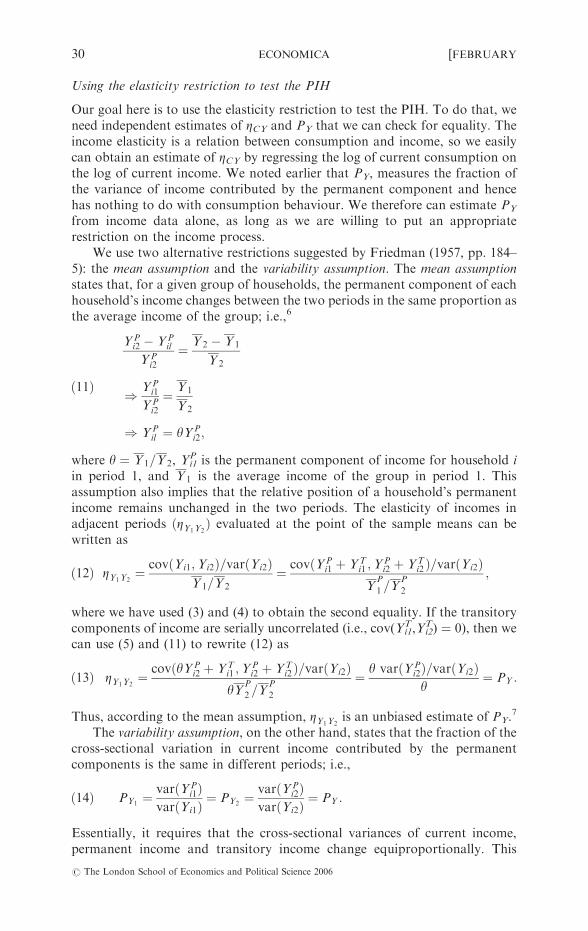
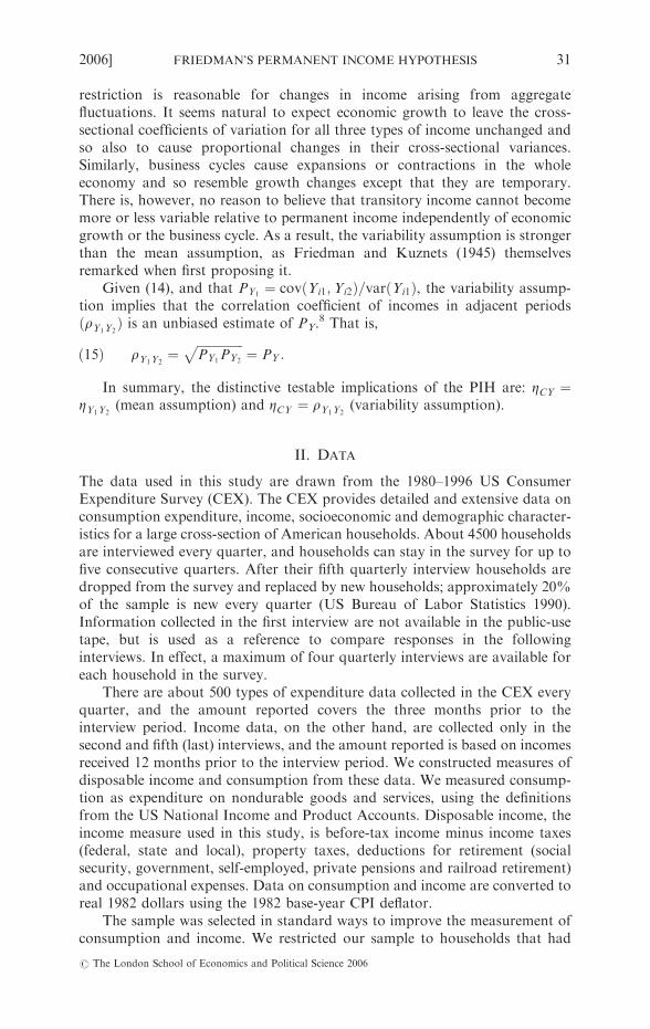
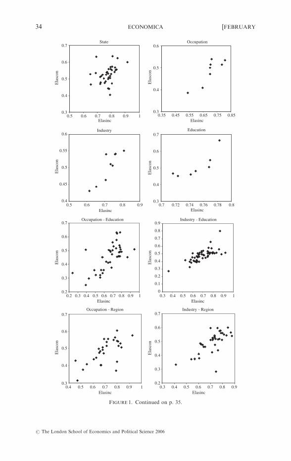
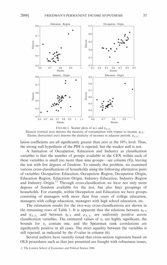
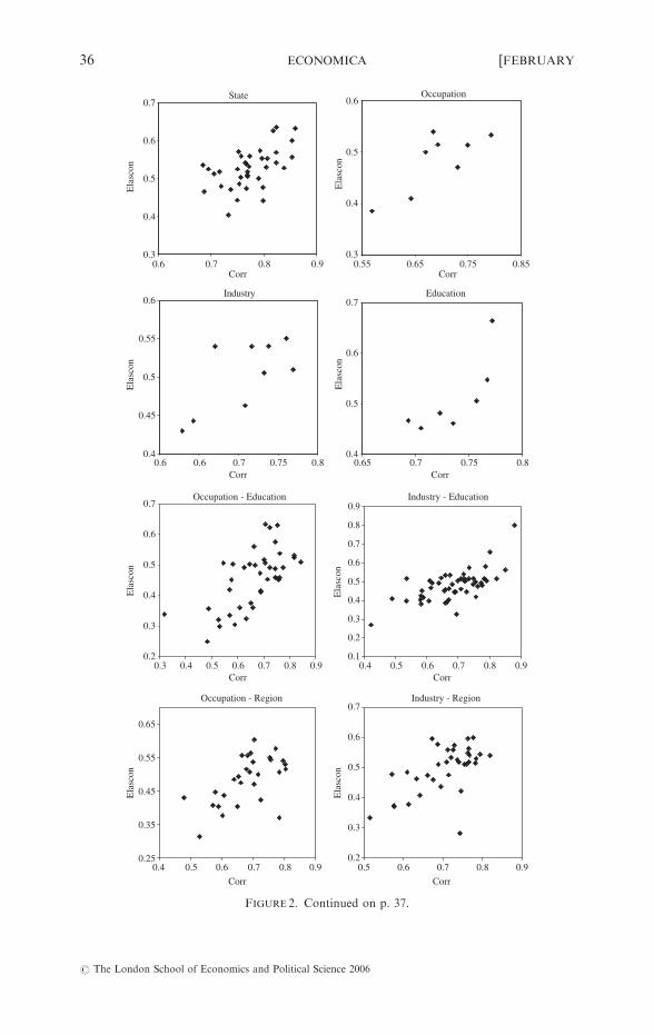
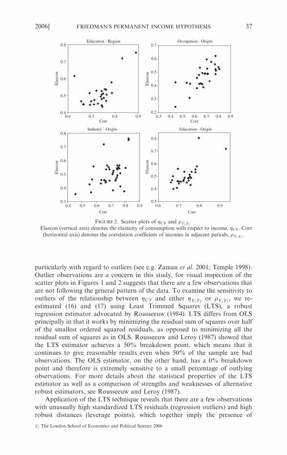
Figures 1 and 2 present scatter plots for each classification variable,showing ZCY plotted against either ZY1Y2

(Figure 1) or rY1Y2(Figure 2).10

Although there are some outliers, the plots clearly indicate a positive relationbetween the variables. To examine the relationship rigorously, we performedtwo types of test: regressions and rank correlations. For the first type of test weestimated the following cross-section regressions:

ð16Þ ZCY ;g ¼ a0 þ a1 ZY1Y2;gþ eg;

ð17Þ ZCY ;g ¼ a0 þ a1 rY1Y2;gþ eg;

where g indexes groups within a classification variable (e.g. managers or clerkswithin occupation), and eg is the group-specific random disturbance term. Thestatistical equivalent of the PIH implication that ZCY equals either ZY1Y2

orrY1Y2

is the joint hypothesis that a0 ¼ 0 and a1 ¼ 1. As mentioned, limitationsof the data may introduce unavoidable biases that would lead to the rejectionof one or both parts of this joint hypothesis. The PIH still implies a positiverelation between ZCY and either ZY1Y2

or rY1Y2, so we also tested the simple

hypothesis that a1 is significantly greater than zero and, if so, whether it isinsignificantly different from one. Furthermore, ZCY, ZY1Y2

and rY1Y2are

estimated parameters and so are subject to estimation error. That alone impliesthat the point estimate of a1 will be biased downward and hence will provideonly an approximate lower-bound estimate for the true value. For this reason,whenever the estimate of a1 was significantly less than one we also performedthe reverse regression of ZY1Y2

on ZCY and/or rY1Y2on ZCY to obtain an

approximate upper bound for a1 (Maddala 1992). Finally, we computed theSpearman rank correlation between ZCY on the one hand and ZY1Y2

and rY1Y2

on the other. This non-parametric statistic is limited to testing for a positiverelation between the variables, but it is attractive because it is robust to boththe functional form of the relation and the distributional properties of the data.

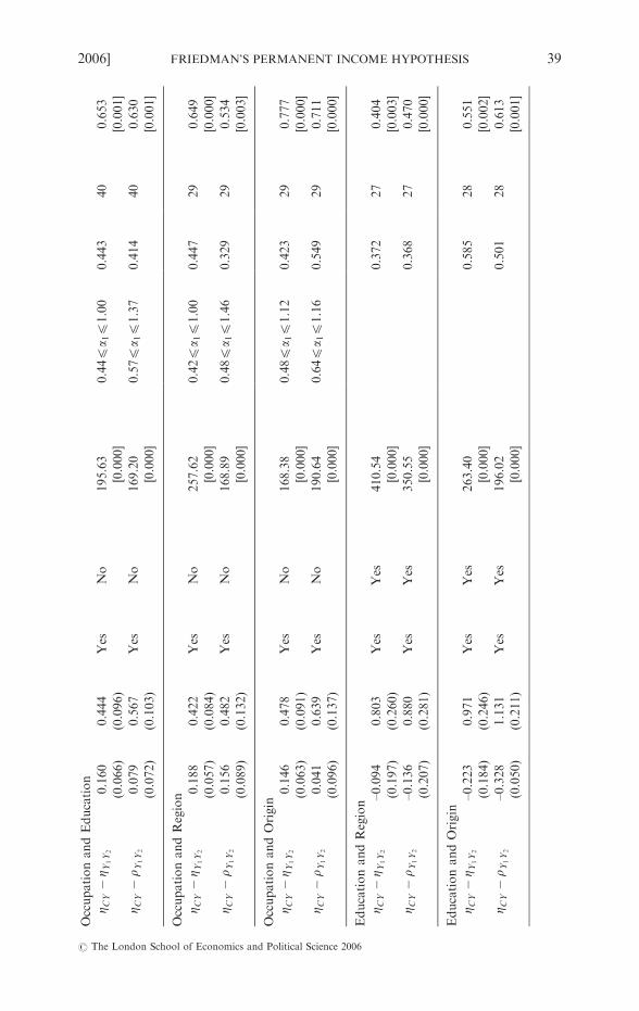
Table 1 reports the cross-section regression estimates of (16) and (17) usingthe ordinary least squares (OLS) procedure. Heteroscedasticity-consistentstandard errors are shown in parentheses. For each classification variable, tworow entries are shown, the first referring to the mean assumption ðZCY � ZY1Y2

Þand the second to the variability assumption ðZCY � rY1Y2

Þ.The results for the Occupation, Industry, Education and State classification

variables are qualitatively similar.11 The joint hypothesis of (a0 ¼ 0, a1 ¼ 1) isrejected; however, the estimated values of a1 are positive and highly significant,ranging from 0.324 (State) to 2.493 (Education), and the estimated bounds for a1include the hypothesis that a1 ¼ 1, except for Education. The Spearman corre-



State

0.3

0.4

0.5

0.6

0.7

0.5 0.6 0.7 0.8 0.9 1Elasinc

Ela

scon

Occupation

0.3

0.4

0.5

0.6

0.35 0.45 0.55 0.65 0.75 0.85Elasinc

Ela

scon

Industry

0.4

0.45

0.5

0.55

0.6

0.5 0.6 0.7 0.8 0.9Elasinc

Ela

scon

Education

0.3

0.4

0.5

0.6

0.7

0.7 0.72 0.74 0.76 0.78 0.8Elasinc

Ela

scon

Occupation - Education

0.2

0.3

0.4

0.5

0.6

0.7

0.2 0.3 0.5 0.6 0.7 0.8 0.9 1Elasinc

Ela

scon

Industry - Education

0

0.1

0.2

0.3

0.4

0.5

0.6

0.7

0.8

0.9

0.3 0.4 0.5 0.6 0.7 0.8 0.9 1Elasinc

Ela

scon

Occupation - Region

0.3

0.4

0.5

0.6

0.7

0.4 0.5 0.6 0.7 0.8 0.9 1Elasinc

Ela

scon

Industry - Region

0.2

0.3

0.4

0.5

0.6

0.7

0.3 0.4 0.5 0.6 0.7 0.8 0.9Elasinc

Ela

scon

0.4

FIGURE 1. Continued on p. 35.



lation coefficients are all significantly greater than zero at the 10% level. Thus,the strong null hypothesis of the PIH is rejected, but the weaker null is not.

A limitation of Occupation, Education and Industry as classificationvariables is that the number of groups available in the CEX within each ofthese variables is small (no more than nine groupsFsee column (9)), leavingthe test with few degrees of freedom. To remedy this problem, we examinedvarious cross-classifications of households using the following alternative pairsof variables: Occupation–Education, Occupation–Region, Occupation–Origin,Education–Region, Education–Origin, Industry–Education, Industry–Regionand Industry–Origin.12 Through cross-classification we have not only moredegrees of freedom available for the test, but also finer groupings ofhouseholds. For example, within Occupation and Education we have groupsconsisting of managers with more than four years of college education,managers with college education, managers with high school education, etc.

The estimation results for the two-way cross-classifications are shown inthe remaining rows of Table 1. It is apparent that the relations between ZCYand ZY1Y2

and between ZCY and rY1Y2are uniformly positive across

classification variables. The estimated values of a1 are highly significant, thebounds for a1 contain one, and the Spearman rank correlations aresignificantly positive in all cases. The strict equality between the variables isstill rejected, as indicated by the F-value in column (6).

Several authors have recently noted that cross-section regression based onOLS procedures such as that just presented are fraught with robustness issues,

Education - Region

0.4

0.5

0.6

0.7

0.8

0.6 0.7 0.8 0.9 1Elasinc

Ela

scon

Occupation - Origin

0.2

0.3

0.4

0.5

0.6

0.7

0.3 0.4 0.5 0.6 0.7 0.8 0.9Elasinc

Ela

scon

Industry - Origin

0.3

0.4

0.5

0.6

0.7

0.8

0.4 0.5 0.6 0.7 0.8 0.9 1 1.1Elasinc

Ela

scon

Education - Origin

0.3

0.4

0.5

0.6

0.7

0.8

0.9

0.6 0.7 0.8 0.9 1Elasinc

Ela

scon

FIGURE 1. Scatter plots of Zcy and ZY1Y2

Elascon (vertical axis) denotes the elasticity of consumption with respect to income, ZCY.Elasinc (horizontal axis) denotes the elasticity of incomes in adjacent periods, ZY1Y2

.



State

0.3

0.4

0.5

0.6

0.7

0.6 0.7 0.8 0.9Corr

Ela

scon

Occupation

0.3

0.4

0.5

0.6

0.55 0.65 0.75 0.85

Ela

scon

Industry

0.4

0.45

0.5

0.55

0.6

0.6 0.6 0.7 0.75 0.8Corr

Ela

scon

Education

0.4

0.5

0.6

0.7

0.65 0.7 0.75 0.8Corr

Ela

scon

Corr

Occupation - Education

0.2

0.3

0.4

0.5

0.6

0.7

0.3 0.4 0.5 0.6 0.7 0.8 0.9

Ela

scon

Industry - Education

0.1

0.2

0.3

0.4

0.5

0.6

0.7

0.8

0.9

0.4 0.5 0.6 0.7 0.8 0.9

Ela

scon

Occupation - Region

0.25

0.35

0.45

0.55

0.65

0.4 0.5 0.6 0.7 0.8 0.9

Ela

scon

Industry - Region

0.2

0.3

0.4

0.5

0.6

0.7

0.5 0.6 0.7 0.8 0.9

Ela

scon

Corr Corr

Corr Corr

FIGURE 2. Continued on p. 37.



particularly with regard to outliers (see e.g. Zaman et al. 2001; Temple 1998).Outlier observations are a concern in this study, for visual inspection of thescatter plots in Figures 1 and 2 suggests that there are a few observations thatare not following the general pattern of the data. To examine the sensitivity tooutliers of the relationship between ZCY and either ZY1Y2

or rY1Y2, we re-

estimated (16) and (17) using Least Trimmed Squares (LTS), a robustregression estimator advocated by Rousseeuw (1984). LTS differs from OLSprincipally in that it works by minimizing the residual sum of squares over halfof the smallest ordered squared residuals, as opposed to minimizing all theresidual sum of squares as in OLS. Rousseeuw and Leroy (1987) showed thatthe LTS estimator achieves a 50% breakdown point, which means that itcontinues to give reasonable results even when 50% of the sample are badobservations. The OLS estimator, on the other hand, has a 0% breakdownpoint and therefore is extremely sensitive to a small percentage of outlyingobservations. For more details about the statistical properties of the LTSestimator as well as a comparison of strengths and weaknesses of alternativerobust estimators, see Rousseeuw and Leroy (1987).

Application of the LTS technique reveals that there are a few observationswith unusually high standardized LTS residuals (regression outliers) and highrobust distances (leverage points), which together imply the presence of

Education - Region

0.4

0.5

0.6

0.7

0.8

0.6 0.7 0.8 0.9

Ela

scon

Occupation - Origin

0.2

0.3

0.4

0.5

0.6

0.7

0.3 0.4 0.5 0.6 0.7 0.8 0.9Corr

Ela

scon

Industry - Origin

0.3

0.4

0.5

0.6

0.7

0.8

0.4 0.5 0.6 0.7 0.8 0.9

Corr

Ela

scon

Education - Origin

0.3

0.4

0.5

0.6

0.7

0.8

0.6 0.7 0.8 0.9

Ela

scon

Corr

Corr

FIGURE 2. Scatter plots of ZCY and rY1Y2

Elascon (vertical axis) denotes the elasticity of consumption with respect to income, ZCY. Corr(horizontal axis) denotes the correlation coefficient of incomes in adjacent periods, rY1Y2

.



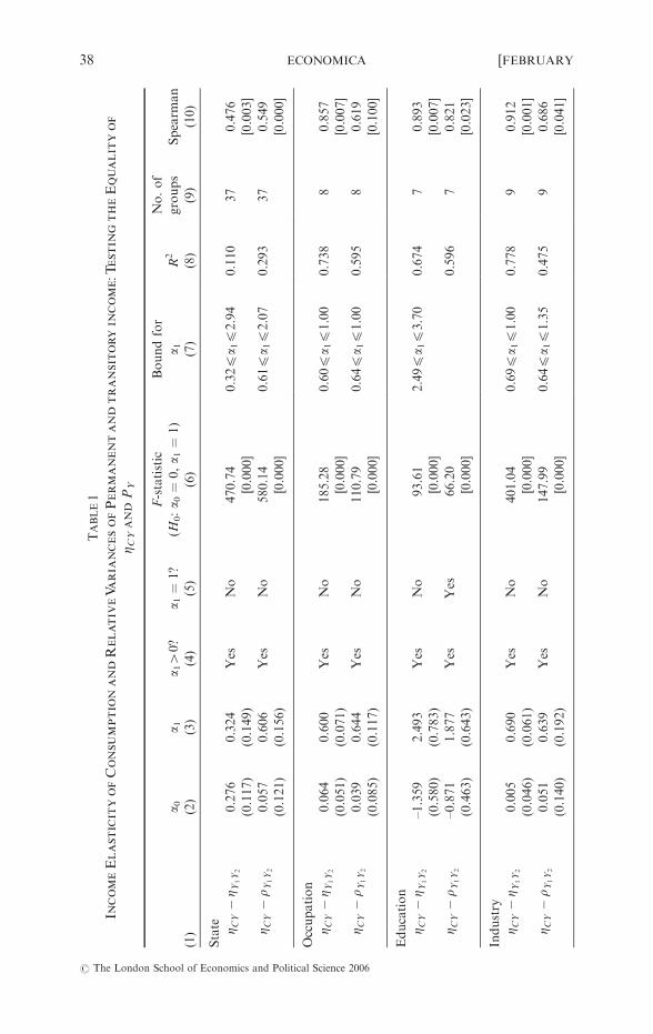
TABLE1

IncomeElasticityofConsumptionandRelativeVariancesofPermanentandtransitoryincome:TestingtheEqualityof

Z CYandPY

a 0a 1

a 140?

a 1¼

1?

F-statistic

(H0:a 0¼

0,a 1¼

1)

Boundfor

a 1R2

No.of

groups

Spearm

an

(1)

(2)

(3)

(4)

(5)

(6)

(7)

(8)

(9)

(10)

State Z CY�Z Y

1Y

20.276

0.324

Yes

No

470.74

0.324

a 142.94

0.110

37

0.476

(0.117)

(0.149)

[0.000]

[0.003]

Z CY�r Y

1Y

20.057

0.606

Yes

No

580.14

0.614

a 142.07

0.293

37

0.549

(0.121)

(0.156)

[0.000]

[0.000]

Occupation

Z CY�Z Y

1Y

20.064

0.600

Yes

No

185.28

0.604

a 141.00

0.738

80.857

(0.051)

(0.071)

[0.000]

[0.007]

Z CY�r Y

1Y

20.039

0.644

Yes

No

110.79

0.644

a 141.00

0.595

80.619

(0.085)

(0.117)

[0.000]

[0.100]

Education

Z CY�Z Y

1Y

2–1.359

2.493

Yes

No

93.61

2.494

a 143.70

0.674

70.893

(0.580)

(0.783)

[0.000]

[0.007]

Z CY�r Y

1Y

2–0.871

1.877

Yes

Yes

66.20

0.596

70.821

(0.463)

(0.643)

[0.000]

[0.023]

Industry

Z CY�Z Y

1Y

20.005

0.690

Yes

No

401.04

0.694

a 141.00

0.778

90.912

(0.046)

(0.061)

[0.000]

[0.001]

Z CY�r Y

1Y

20.051

0.639

Yes

No

147.99

0.644

a 141.35

0.475

90.686

(0.140)

(0.192)

[0.000]

[0.041]



OccupationandEducation

Z CY�Z Y

1Y

20.160

0.444

Yes

No

195.63

0.444

a 141.00

0.443

40

0.653

(0.066)

(0.096)

[0.000]

[0.001]

Z CY�r Y

1Y

20.079

0.567

Yes

No

169.20

0.574

a 141.37

0.414

40

0.630

(0.072)

(0.103)

[0.000]

[0.001]

OccupationandRegion

Z CY�Z Y

1Y

20.188

0.422

Yes

No

257.62

0.424

a 141.00

0.447

29

0.649

(0.057)

(0.084)

[0.000]

[0.000]

Z CY�r Y

1Y

20.156

0.482

Yes

No

168.89

0.484

a 141.46

0.329

29

0.534

(0.089)

(0.132)

[0.000]

[0.003]

OccupationandOrigin

Z CY�Z Y

1Y

20.146

0.478

Yes

No

168.38

0.484

a 141.12

0.423

29

0.777

(0.063)

(0.091)

[0.000]

[0.000]

Z CY�r Y

1Y

20.041

0.639

Yes

No

190.64

0.644

a 141.16

0.549

29

0.711

(0.096)

(0.137)

[0.000]

[0.000]

EducationandRegion

Z CY�Z Y

1Y

2–0.094

0.803

Yes

Yes

410.54

0.372

27

0.404

(0.197)

(0.260)

[0.000]

[0.003]

Z CY�r Y

1Y

2–0.136

0.880

Yes

Yes

350.55

0.368

27

0.470

(0.207)

(0.281)

[0.000]

[0.000]

EducationandOrigin

Z CY�Z Y

1Y

2–0.223

0.971

Yes

Yes

263.40

0.585

28

0.551

(0.184)

(0.246)

[0.000]

[0.002]

Z CY�r Y

1Y

2–0.328

1.131

Yes

Yes

196.02

0.501

28

0.613

(0.050)

(0.211)

[0.000]

[0.001]



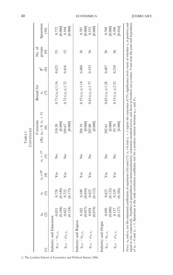
TABLE1

CONTIN

UED

a 0a 1

a 140?

a 1¼

1?

F-statistic

(H0:a 0¼

0,a 1¼

1)

Boundfor

a 1R2

No.of

groups

Spearm

an

(1)

(2)

(3)

(4)

(5)

(6)

(7)

(8)

(9)

(10)

Industry

andEducation

Z CY�Z Y

1Y2

–0.031

0.728

Yes

No

310.50

0.734

a 141.16

0.623

53

0.772

(0.104)

(0.149)

[0.000]

[0.000]

Z CY�r Y

1Y

2–0.022

0.722

Yes

No

189.67

0.724

a 141.72

0.418

53

0.594

(0.124)

(0.173)

[0.000]

[0.000]

Industry

andRegion

Z CY�Z Y

1Y2

0.102

0.549

Yes

No

288.19

0.554

a 141.14

0.480

36

0.707

(0.037)

(0.054)

[0.000]

[0.000]

Z CY�r Y

1Y

20.054

0.625

Yes

No

203.00

0.634

a 141.77

0.353

36

0.552

(0.079)

(0.112)

[0.000]

[0.000]

Industry

andOrigin

Z CY�Z Y

1Y2

0.050

0.623

Yes

No

202.61

0.624

a 141.28

0.487

36

0.708

(0.090)

(0.132)

[0.000]

[0.000]

Z CY�r Y

1Y

20.137

0.529

Yes

No

95.70

0.534

a 142.52

0.210

36

0.398

(0.127)

(0.188)

[0.000]

[0.016]

Notes:

a 0anda 1

are

theestimatedcoefficientsofequations(16)and(17).a 140anda 1¼

1reporttheoutcomes

of5%

significance

levelt-testsofwhether

a 1ispositiveand

equalto

one,respectively.Numbersin

parentheses

are

heteroscedasticity–consistentstandard

errors,andthose

inbracketsare

p-values.F-statteststhejointnullhypothesis

ofa 0¼

0anda 1¼

1.Spearm

anistherankcorrelationcoefficienttest

forapositiverelationbetweenZ C

YandPY.



influential outliers or so-called bad leverage points. Specifically, threeclassification groups have three influential outliers, three groups have twooutliers, six groups have one outlier and the remaining 12 groups have noinfluential outlier. Following the recommendation of Rousseeuw, we ran OLSwithout these influential outliers to obtain the robustly fitted regression line.The results are nearly the same as the OLS results in Table 1. The robustregression fits are slightly better, and the estimates of a1 are marginally larger,giving rise to narrower bounds for a1. Accounting for outliers thus increasesboth the magnitude and the precision of the point estimate of a1. The estimatesof a1 are positive and highly significant. None the less, a1 remains significantlydifferent from one (except for a few cases), and the joint hypothesis (a0 ¼ 0,a1 ¼ 1) continues to be rejected. All in all, outliers do not seriously alter ourearlier results.13

The overall conclusions from our tests are that both the parametric(regression-based) and non-parametric (Spearman rank correlation) testssupport the implication of the PIH that ZCY is positively correlated withZY1Y2

or rY1Y2. The strongest implications of the PIHFthat a1 individually

equals one and that a0 and a1 satisfy the joint hypothesis (a0 ¼ 0, a1 ¼ 1)Farerejected.

IV. CONCLUDING REMARKS

In this paper, we use modern US household data from the 1980–96 ConsumerExpenditure Survey to test a key implication of Permanent Income Hypothesis(PIH) as originally advanced by Friedman (1957), namely that the incomeelasticity of consumption should be higher for households for which a largefraction of the variation of their income is permanent than for householdsfacing more transitory variations in income. Our data are far superior to whatwas available to Friedman, allowing us to check statistical significance andconduct tests he could not perform.

Reassessing Friedman’s test is interesting and useful both substantively andhistorically. On the substantive side, the test is simple but intuitive, and clearlydifferent from either the Euler equation tests or the older consumptionfunction tests; they therefore increase the dimensionality of the battery of testsof the PIH, which in turn increases the robustness of the overall set of testsavailable. On the historical side, the test revives the use of clever insights intothe nature of the PIH by its founder.

In terms of the substantive results, our test results support the PIH andthus complement the other tests of the PIH based on micro data such asRunkle (1991), Attanasio and Weber (1995) and DeJuan and Seater (1999),which also offer support to the PIH. However, the strongest implicationsof the PIH are rejected, a result that deserves further exploration. We regardour reassessment of Friedman’s original PIH test as promising, not onlybecause of its implications regarding possible validity of the PIH, but moreimportantly because it suggests useful avenues for further research, and simplybecause it is interesting to see how old ideas fare when confronting new data.Friedman’s old ideas are not obviously outmoded, and that is indeed aninteresting result.



APPENDIX

Effects of measurement error

As noted in Section II, measurement error affects the estimates of ZCY, ZY1Y2and rY1Y2

equally, so that the test for equality of ZCY to either ZY1Y2or rY1Y2

is not biased for oragainst the PIH. To show this, we first need to examine the effects of measurement erroron the income elasticity of consumption, ZCY, which is estimated by the slope coefficientof the regression of the log of current consumption on the log of current income.

Designate the true levels of current consumption and current income for householdi by Cn

i and Yni and the measured levels by Ci and Yi, so that

ðA1Þ Ci ¼ Cni Ui;

ðA2Þ Yi ¼ Yni Vi;

where Ui and Vi represent measurement errors. The characteristics of the measurementerrors are assumed to be

ðA3Þ logUi ¼ ui � Nð0; s2uÞ;

ðA4Þ logVi ¼ vi � Nð0; s2vÞ;

ðA5Þ EðuiviÞ ¼ 0;

ðA6Þ EðuiuiþjÞ ¼ 0 for j 6¼ 0;

ðA7Þ EðviviþjÞ ¼ 0 for j 6¼ 0:

These assumptions state that each error is a log-normal random variable with zeromean and constant variance. The assumptions also rule out autocorrelation in theerrors.

In the presence of measurement error, the regression of log Cn on log Yn becomes

ðA8Þ ðci � uiÞ ¼ ZCY ðyi � viÞ þ ei;

where (ci � ui) ¼ (logCi � logUi) and (yi � vi) is defined analogously. Rearranging termsgives

ðA9Þ ci ¼ ZCYyi þ wi;

where ZCY is the slope coefficient or the income elasticity of consumption, andwi ¼ ei þ ui � ZCYvi is the compound error term. Let ZCY denote the OLS estimate ofZCY. Using least squares algebra, we have

ðA10Þ ZCY ¼P

ciyiPy2i¼Pðcni þ uiÞðyni þ viÞPðyni þ viÞ2

;

ðA11Þ p lim ZCY ¼covðcn; ynÞ

varðynÞ þ varðvÞ ¼scnyn

s2yn þ s2v:

Since ZCY ¼ scnyn=s2yn , we can rewrite p lim ZCY as

ðA12Þ p lim ZCY ¼ZCY

1þ s2v=s2yn:

Thus, ZCY will underestimate ZCY as a result of measurement error in Y.Now, let us examine the effects of measurement error on the elasticity of incomes in

adjacent periods ZY1Y2, which is estimated by the slope coefficient of the regression of the

log of previous period income on the log of current period income. (Note that we are



referring to Y2 as the current-period income and Y1 as the previous-period income.) Tosimplify notation, designate Y1 by Z and Y2 by Y so we can rewrite ZY1Y2

as ZZY. Asbefore, let variables with and without asterisks denote the true and observed values, sothat

ðA13Þ Zi ¼ Zni Qi;

ðA14Þ Yi ¼ Yni Vi;

where Vi and Qi represent measurement error. The characteristics of the measurementerrors are assumed to be

ðA15Þ logQi ¼ qi � Nð0; s2qÞ;

ðA16Þ logVi ¼ vi � Nð0; s2vÞ;

ðA17Þ EðviqiÞ ¼ 0;

ðA18Þ Eðqi qiþjÞ ¼ 0 for j 6¼ 0;

ðA19Þ Eðvi viþjÞ ¼ 0 for j 6¼ 0:

In the presence of measurement error, the regression of logZn on logYn becomes

ðA20Þ ðzi � qiÞ ¼ ZZY ðyi � viÞ þ ei;

where (zi � qi) ¼ (logZi � logQi) and (yi � vi) is defined analogously. Rearranging termsgives

ðA21Þ zi ¼ ZZY yi þ ni;

where ZZY is the slope coefficient or the elasticity of incomes in adjacent periods, andni ¼ ei þ q � ZZYvi is the compound error term. Let ZZY denote the OLS estimate ofZZY. Using least squares algebra, we have

ðA22Þ ZZY ¼P

ziyiPy2i¼Pðzni þ qiÞðyni þ viÞPðyni þ viÞ2

;

ðA23Þ p lim ZZY ¼covðzn; ynÞ

varðynÞ þ varðvÞ ¼sznyn

s2yn þ s2v:

Since ZZY ¼ sznyn=s2yn , we can rewrite p lim ZZY as

ðA24Þ p lim ZZY ¼ZZY

1þ s2v=s2yn:

Thus, ZZY will underestimate ZZY as a result of measurement error in Y.Overall, we can see that the degree of underestimation in (A12) and (A24) depends

on the same factor s2v=s2yn . In this regard, measurement error in Y will not bias the test of

equality of ZCY and ZZY for/against the mean assumption of the PIH.For the variability assumption, the results are the same as long as we suppose that

the variance of the measurement error increases in proportion with the variance ofincome, which certainly is reasonable for changes in income arising from macro-economic sources and is perhaps acceptable for other sources of change in income aswell. In that case, the regression coefficient obtained from the variability assumption isthe coefficient obtained under the mean assumption but multiplied by the ratio ofstandard errors of the two income terms. If the measurement-error standard errorsincrease in the same proportion as the income standard errors, then the ratio in questionis unaffected by the presence of measurement error.



ACKNOWLEDGMENTS

We would like to thank Alastair Hall, Alan Manning and an anonymous referee fortheir helpful comments and suggestions on an earlier version of this paper.

NOTES

1. Equivalently, permanent income is the hypothetical constant value of income having thesame present value as the expected actual income stream.

2. Its absence is notable, for example, in Deaton’s (1992) superb review of the empiricalliterature on consumption.

3. In many early tests of the PIH, including Friedman’s (1957), the data on consumption arederived by subtracting saving from income. If saving is measured with error, this procedurecreates a common error term in income and consumption, leading to a biased test of thePIH.

4. Aggregate shocks can cause the sum of transitory components to be non-zero in any giventime period. As we discuss later, we avoided this problem by using a pooled cross-section ofhouseholds over 1980–96, a 17-year period that included three recessions and sixconsecutive years of high real growth. We expected aggregate shocks to have largelyaveraged out over such a long period.

5. Of the three correlations in (5), the third seems most controversial. It says that transitoryconsumption and transitory income are not correlated across households. Empiricalattempts to test this assumption based on household data have obtained mixed results.Bodkin (1959) found large marginal propensity to consume (MPC) from the NationalService Life Insurance dividend payments paid to Second World War veterans in 1950, butFriedman (1960) noted that the dividend payments may be correlated with omittedvariables that are in turn correlated with permanent income (i.e. omitted variable bias), sothat Bodkin’s estimated MPC of dividend payments is upwardly biased. Bird and Bodkin(1965) subsequently re-estimated the consumption function with measures of permanentincome included. They found a relatively small MPC and concluded that the results wereconsistent with the PIH. In a similar study, Kreinin (1961) examined the consumptionbehaviour of Israeli recipients of Second World War lump-sum personal restitutionpayments from Germany and found the MPC out of restitution payments insignificantlydifferent from zero. Recent papers using the Euler equation framework have examined arelated issue about the response of household consumption to a particular type of incomethat is both predictable and transitory, e.g. income tax refunds and income tax cuts. Theresults in Browning and Collado (2001) and Hsieh (2003), among others, found thatconsumption expenditures do not overreact to this type of income change; whereas Parker(1999) and Souleles (1999) found some overreactions.

6. Suppose we group households by their occupationFmanagers, craftsmen, farmers, etc.Among craftsmen, for example, the mean assumption maintains that, on average, thepermanent component of each craftsman’s income should change in the same proportion asthe average income of all craftsmen.

7. If the transitory components of income are serially correlated, then ZY1Y2would be a biased

estimate of PY. However, ZY1Ydwill be an unbiased estimate of PY for d sufficiently large

that the transitory component in period d is uncorrelated with that in period 1. Carroll andSamwick (1997, 1998) addressed the issue of serial correlation in the transitory componentby using the d-year income difference panel data in their estimation of the variances of thepermanent and transitory components of income. In contrast to Carroll and Samwick’sdata, our data-set has only two income observations per household, making it impossiblefor us to check if our results are sensitive to the choice of d. If the transitory components areserially correlated, then we would expect the estimate of ZY1Y2

to overestimate the true PY,and strict equality of ZCY and ZY1Y2

might be rejected by the data. None the less, asdiscussed later, ZCY and ZY1Y2

are still expected to be positively correlated if the PIH is true.8. The estimate of rY1Y2

will be subject to the same bias noted in footnote 7 if the transitorycomponents of income are serially correlated.

9. For Occupation, the categories available in the CEX are Managerial and professionalspecialty; Technical, sales and administrative support; Service; Farming, forestry andfishing; Precision production, craft and repair; Operators, fabricators and labourers; Armedforces; and Self-employed. For Industry, the categories are Agriculture, forestry, fisheriesand mining; Construction; Manufacturing; Transportation, communications and otherpublic utilities; Wholesale and retail trade; Finance, insurance and real estate; Professionaland related services; Other services; and Public administration. For Education, thecategories are Elementary; Less than high school; High school graduate; Less than college



graduate; College graduate; More than 4 years of college; Never attended school. For State,data are available only for the 37 most populous US states.

10. Results are qualitatively similar to those reported here if income is conditioned on age andtime (i.e., variables that vary deterministically over the life cycle) and then the analysis isconducted on the residuals after controlling for such variables.

11. The issue of self-selection arises when using classification variables such as Occupation andIndustry. However, it should be noted that our test here concerns the information value ofcurrent income fluctuations. Irrespective of the reason why the household chose to be amanager or a farmer, its consumption according to the PIH should respond less to currentincome fluctuations if those represent transitory rather than permanent income variation.The test therefore seems free of selection bias, at least on this account. Of course, it is notpossible to guarantee total absence of selection bias for any classification variables, so weexamine several alternative variables and judge the weight of the evidence. Note that someclassification variables we use, such as education and state (the part of the country whereone lives), are less likely to be subject to selection bias.

12. The Origin variable is categorized in the CEX as European, Spanish and Afro-American.For Region, they are Northeast, Midwest, South and West. Ideally, we would have cross-classified the households using more than two variables, but doing so would have decreaseddramatically the number of observations in each household group, leading to impreciseestimates of ZCY, ZY1Y2

and rY1Y2.

13. The robust estimation results are available from the authors upon request.

REFERENCES

ATTANASIO, O. and WEBER, G. (1995). Is consumption growth consistent with intertemporal

optimization? Evidence from the consumer expenditure survey. Journal of Political Economy,

103, 1121–57.

BIRD, R. and BODKIN, R. (1965). The national service life insurance dividend of 1950 and

consumption: a further test of the ‘strict’ permanent income hypothesis. Journal of Political

Economy, 73, 499–515.

BODKIN, R. (1959). Windfall income and consumption. American Economic Review, 49, 602–14.

BROWNING, M. and COLLADO, M. (2001). The response of expenditures to anticipated income

changes: panel data estimates. American Economic Review, 91, 681–92.

CARROLL, C. and SAMWICK, A. (1997). The nature of precautionary wealth. Journal of Monetary

Economics, 40, 41–71.

FFF and FFF (1998). How important is precautionary saving? Review of Economics and

Statistics, 80, 410–19.

DEATON, A. (1992). Understanding Consumption. Oxford: Oxford University Press.

DEJUAN, J. and SEATER, J. (1999). The Permanent Income Hypothesis: evidence from the

consumer expenditure survey. Journal of Monetary Economics, 43, 351–76.

FRIEDMAN, M. (1957). A Theory of the Consumption Function. Princeton: Princeton University

Press.

FFF (1960). Comments. In I. Friend and R. Jones (eds.), Proceedings of the Conference in

Consumption and Savings, vol. 2. Philadelphia: University of Pennsylvania Press.

FFF and KUZNETS, S. (1945). Income from Independent Professional Practice. New York:

National Bureau of Economic Research.

HSIEH, C. (2003). Do consumers react to anticipated income shocks? Evidence from the Alaska

Permanent Fund. American Economic Review, 93, 397–405.

KREININ, M. (1961). Windfall income and consumption: additional evidence. American Economic

Review, 51, 388–90.

MADDALA, G. (1992). Introduction to Econometrics, 2nd edn. Englewood Cliffs, NJ: Prentice-Hall.

PARKER, J. (1999). The reaction of household consumption to predictable changes in social security

taxes. American Economic Review, 89, 959–73.

ROUSSEEUW, P. (1984). Least median of squares regression. Journal of the American Statistical

Association, 79, 871–80.

FFF and LEROY, A. (1987). Robust Regression and Outlier Detection. New York: John Wiley.

RUNKLE, D. (1991). Liquidity constraints and the permanent income hypothesis. Journal of

Monetary Economics, 27, 73–98.



SOULELES, N. (1999). The response of household consumption to income tax refunds. American

Economic Review, 89, 947–58.

TEMPLE, J. (1998). Robustness tests of the augmented Solow model. Journal of Applied

Econometrics, 13, 361–75.

US BUREAU OF LABOR STATISTICS (1980). Consumer Expenditure Survey: Interview Survey 1980–

1996. Public Use Tapes.

ZAMAN, A., ROUSSEEUW, P. and ORHAN, M. (2001). Econometric applications of high-breakdown

robust regression techniques. Economics Letters, 71, 1–8.



Documents

A Simple Test of Friedman’s Permanent Income Hypothesisjjseater/simpletest.pdf · A Simple Test of Friedman’s Permanent Income Hypothesis ... many powerful implications, ... brief