BUFFER-STOCK SAVING AND THE LIFE CYCLE/PERMANENT INCOME HYPOTHESIS*

Published in the Quarterly Journal of Economics

1997(1), Volume CXII, Pages 1-56

Christopher D. Carroll Johns Hopkins University

ccarroll@jhu.edu

First Draft: July, 1990 This Draft: August 13, 1996

Abstract This paper argues that the typical household’s saving is better described by a “buffer-stock” version than by the traditional version of the Life Cycle/Permanent Income Hypothesis (LC/PIH) model. Buffer-stock behavior emerges if consumers with important income uncertainty are sufficiently impatient. In the traditional model, consumption growth is determined solely by tastes; in contrast, buffer-stock consumers set average consumption growth equal to average labor income growth, regardless of tastes. The model can explain three empirical puzzles: the “consumption/income parallel” of Carroll and Summers [1991]; the “consumption/income divergence” first documented in the 1930's; and the temporal stability of the household age/wealth profile despite the unpredictability of idiosyncratic wealth changes.

Keywords: consumption, saving, precautionary saving, buffer-stock saving, uncertainty JEL Codes: D91 E21 *Thanks to Olivier Blanchard, Sean Craig, Angus Deaton, Karen Dynan, Eric Engen, John Gruber, Miles Kimball, James Poterba, Ranil Salgado, Lawrence Summers, Jonathan Skinner, David Weil, David Wilcox, Stephen Zeldes, and the members of the MIT Money and Public Finance lunches for constructive comments. Remaining errors are my own.

- 1 -

I. Introduction

Of the consumers who participated in the Federal Reserve Board's 1983 Survey of

Consumer Finances, 43 percent said that being prepared for emergencies was the most

important reason for saving. Only 15 percent said that preparing for retirement was the most

important saving motive.1 These are not the answers that standard interpretations of the Life

Cycle/Permanent Income Hypothesis (LC/PIH) model of saving would lead one to expect.

This paper will argue, however, that such responses, and a wide range of other evidence,

are consistent with a version of the LC/PIH model in which consumers face important income

uncertainty, but are also both “prudent,” in Miles Kimball’s [1990b] sense that they have a

precautionary saving motive, and “impatient” in the sense that if future income were known with

certainty they would choose to consume more than their current income.2 Under these

conditions, consumers may engage in what I call “buffer-stock” saving behavior.3 Buffer-stock

savers have a target wealth-to-permanent-income ratio such that, if wealth is below the target, the

precautionary saving motive will dominate impatience and the consumer will save, while if

wealth is above the target, impatience will dominate prudence and the consumer will dissave.4

I first describe the main properties of the buffer-stock model in an infinite-horizon

context where labor income growth is constant. The model’s most surprising feature is its

implication that, even with a fixed aggregate interest rate, if consumers are sufficiently

“impatient,” average consumption growth will equal average labor income growth, either for

individual households or for aggregate consumption.5 This is true even though the consumers in

1 Summarized in Avery and Kennickell [1989]. The other possible categories were "To buy something or for the family" (29%), and "Investment" (7%). Later SCF surveys produced similar results. 2 This desire to borrow can be due either to a high time preference rate or to high expected income growth. 3 Prudence, in Kimball’s sense of having a utility function with a positive third derivative, is not by itself sufficient to generate buffer-stock saving. The utility function must also exhibit Decreasing Absolute Prudence, as does the Constant Relative Risk Aversion (CRRA) utility function used in this paper. See Kimball [1990a, 1990b] for arguments that Decreasing Absolute Prudence is a natural condition to require of utility functions. 4 The proof that a target wealth-to-income ratio exists, and is stable, is contained, along with many other derivations and proofs, in a companion paper to this one, Carroll [1996]. For a copy of that paper, contact the author. 5 Standard general equilibrium models imply the economy will converge to a steady-state in which the growth rate of consumption equals the growth rate of income. However, the mechanism by which this is achieved is through the dependence of the interest rate on the capital stock; in the model considered here, this channel is short-circuited by assuming a fixed aggregate

- 2 -

the model behave according to the standard Euler equation which has been widely thought to

imply that consumption growth depends only on tastes, and not on the growth rate of income.

The problem in previous work has been in the common assumption that the second-order

variance term in the log-linearized version of the Euler equation can safely be ignored. In fact,

this variance term is an endogenous equilibrating variable: it will, on average, take on whatever

value is required to cause average consumption growth to equal average income growth.

I also present simulation evidence documenting other major differences between

implications of the buffer-stock model and what I will refer to as the “standard” model (either the

perfect-certainty model with Constant Relative Risk Aversion utility, or the Certainty Equivalent

(CEQ) model in which utility is quadratic). In comparison with the standard model, the buffer-

stock model predicts a much higher marginal propensity to consume out of transitory income, a

much higher effective discount rate for future labor income, and a positive rather than negative

sign for the correlation between saving and expected labor income growth.

Whether these results for the infinite-horizon model carry over to the finite-horizon

context cannot be determined analytically. The next section of the paper therefore solves a

finite-horizon version of the model under the same baseline parameter values used in the infinite-

horizon model, but with age/income profiles roughly calibrated to U.S. household-level data. I

show that this configuration of the model generates buffer-stock saving behavior over most of

the working lifetime until roughly age 45 or 50, and behavior that resembles the “standard”

LC/PIH model only for roughly the period between age 50 and retirement.

I then argue that the finite-horizon version of the model can explain three major stylized

facts which, combined, cannot be explained by the principal alternative models: the “standard”

LC/PIH model, a Keynesian alternative to the standard LC/PIH framework, or the Campbell and

Mankiw [1989] combination of these two models. First of the three stylized facts is the

“consumption/income parallel” documented by Carroll and Summers [1991] and Carroll [1994]:

when consumption is aggregated by groups or by whole economies it closely parallels growth in

income over periods of more than a few years. The consumption/income parallel, inconsistent

interest rate.

- 3 -

with the standard LC/PIH framework, is explained in the buffer-stock model as the result of

consumers’ impatience and their prudent unwillingness to borrow. The second fact is the

“consumption/income divergence” that emerges from microeconomic consumer surveys: For

individual households, consumption is often far from current income, implying that the aggregate

consumption/income parallel does not arise from high frequency tracking of consumption to

income at the household level. The consumption/income divergence, inconsistent with the

Keynesian model, is explained with essentially the same logic Friedman used long ago:

consumption does not respond one-for-one to transitory shocks to income because assets are

used to buffer consumption against such shocks.

The final set of stylized facts is about the patterns of wealth accumulation over the

lifetime. I show that the standard LC/PIH model implies that the productivity growth slowdown

after 1973 should have resulted in massive increases in household wealth-income ratios (because

slower expected growth implies lower current consumption). I then demonstrate that the modest

observed changes in the actual age/median-wealth profile match the predictions of the buffer-

stock model. Finally, I argue that the extraordinarily high volatility [Avery and Kennickell,

1989] of household liquid wealth is difficult to explain with either the LC/PIH or the Keynesian

models, but is a natural implication of a model in which the principal purpose of holding wealth

is so that it can be used to absorb random shocks to income.

Although the implications of the buffer-stock version of the LC/PIH model differ in

important respects from standard modern versions of the LC/PIH model, careful reading of

Friedman [1957] suggests that the buffer-stock version of the model represents a close

approximation to his original ideas. Direct quotations from Friedman will illustrate the

similarities between his views and the implications of the buffer-stock model, and some of the

empirical discussion will parallel arguments that Friedman used long ago to justify his

conception of the Permanent Income Hypothesis.

The emphasis on Friedman is not meant to suggest that there has been no progress since

his book. The buffer-stock model presented here owes much to the insights of Kimball

[1990a,b], Zeldes [1989a], and Deaton [1991], who have all emphasized the importance of

precautionary motives for saving. Indeed, the model presented here is structurally similar to the

- 4 -

model of Zeldes [1989a], with the important difference that I assume impatient consumers.

Alternatively, the model is similar to Deaton’s [1991] except that I do not directly impose

liquidity constraints and my model has independent transitory and permanent shocks.

The rest of the paper is organized as follows. Section II sets forth the basic intertemporal

optimization model, briefly describes the method of solution, discusses parametric assumptions,

and, for reference purposes, presents what I will call the “standard” LC/PIH model. Section III

describes the solution to the infinite-horizon version of the model. Section IV presents the finite-

life solution to the model under age/income profiles calibrated from US data and argues that the

resulting behavior fits the stylized facts about household consumption, saving, and wealth better

than the alternative models. Section V contains a brief discussion the recent literature on models

related to the buffer-stock model, and Section VI concludes.

II. The Basic Model

II. A. Solving The Model

I assume that the consumer solves the intertemporal optimization problem:

T (1) max Et ∑ � i-t u(Ci) i=t

such that Wt+1 = R[Wt + Yt - Ct]

Yt = Pt Vt

Pt = Gt Pt-1 Nt,

where Y is current labor income; P is “permanent labor income” defined as the labor income

that would be received if the white noise multiplicative transitory shock to income, V, were

equal to its mean value of one; N is a lognormally distributed white noise mean one

multiplicative shock to permanent income; G = (1+g) is the growth factor for permanent labor

income; W is the stock of physical net wealth; R = (1+r) is the (constant) gross interest rate; and � = 1/(1+� ) is the discount factor where � is the discount rate.

Optimal consumption in any period will depend on total current resources (or “gross

- 5 -

wealth”), the sum of current assets and current income, which, following Deaton [1991], I will

call X:

(2) Xt = Wt + Yt.

The evolution of gross wealth is given by:

(3) Xt+1 = R[Xt - Ct] + Yt+1.

Carroll [1996] demonstrates that this problem can be rewritten by dividing through all variables

by the level of permanent labor income. Defining lower case variables as the upper case variable divided by the current level of permanent income (i.e. ct = Ct/Pt), the general Euler equation for

consumption then becomes:

(4) 1 = R� Et-1 [{ ct[R [xt-1 - ct-1] / G Nt + Vt] GNt / ct-1 } -� ]

In the last period of life, it is optimal to consume everything, cT[xT] = xT. Thereafter,

recursion on equation (4) implicitly defines a rule for the consumption ratio as a function of the

gross wealth ratio in each period back to the beginning of life. Unfortunately, under general

forms of income uncertainty the consumption rules do not have analytical formulas, so they must

be approximated by numerical methods. The details of the method of numerical solution are

contained in Appendix I.

II. B. Parameter Values

I will solve the model and present most of my results for a single baseline set of

parameter values, but will also present a summary of results for alternative choices of all

parameter values so that readers who differ with any particular parametric choice can determine

how sensitive my results are to changes in that parameter. The baseline values for characterizing

the distribution of income shocks will be the same as in Carroll [1992]; using data from the

Panel Study of Income Dynamics, that paper found that household income uncertainly was well

- 6 -

captured by a process that took the form:

V ~

0

Z

with probability p

with probability (1-p) ,

ln Z ~ TN( �� 2

ln Z/2, � 2ln Z),

ln N ~ TN( �� 2ln N/2, � 2

ln N),

where TN signifies a truncated normal distribution (in practice, I truncate at three standard deviations above and below the mean), and � ln Z is chosen to make Et Vt+1 = 1. The choice of

mean for ln N was similarly motivated by the wish to make Et Nt+1 = 1 regardless of the choice

of � 2ln N; this simplifies the analysis of the effect of changes in � 2

ln N on wealth. The probability

of zero income was estimated at about p=0.5 percent per year, and the standard deviation of both

transitory and permanent income shocks were estimated to be around 0.1 percent per year, after

crudely accounting for the effects of measurement error.

The expected growth rate of labor income appropriate for calibrating this model is the

growth rate in household labor income for working households. Carroll and Summers [1991]

provide evidence that, over long periods, household income growth can be characterized as the

sum of aggregate productivity growth and a household-specific component that reflects such

factors as increasing job tenure, seniority, and experience. If we assume very conservatively that

each of these factors contributes 1 percent annually to household income growth, the appropriate

baseline assumption for the growth rate of household labor income is 2 percent per year; this will

be the baseline assumption for the infinite-horizon version of the model. For the finite-horizon

version of the model used later, the pattern of income growth over the lifetime will be calibrated

explicitly using household data.

Carroll [1992] made the strong assumption that the time preference rate was 10 percent

per year; this is a substantial departure from common assumptions in the economic literature.

Much macroeconomic research assumes a discount rate of one percent per quarter, or about 4

- 7 -

percent per year.6 In order to emphasize that the results obtained in this paper are not the result

of extreme assumptions about the time preference rate, the baseline value of the discount rate

assumed in this paper will be 4 percent per year.7

The baseline interest rate will be zero, also following Carroll [1992]. The asset in this

model is perfectly riskless and perfectly liquid; the closest proxy is probably the three-month T-

bill, whose after-tax rate of return over the postwar period has been roughly zero. Results for

interest rates of two percent and four percent are qualitatively similar, and will be presented

later.8

Estimates of the coefficient of relative risk aversion vary widely. Empirical estimates

above 6 have often been obtained (see, e.g., Mankiw and Zeldes [1991]),9 but many economists

believe that values above about 5 imply greater risk aversion than is plausible. At the other extreme, log utility, which is the limit of the CRRA utility function as � approaches one, is a

common assumption because under some circumstances it is analytically tractable. The baseline value of � for this paper will be � = 2, toward the low end of the usual range in order to avoid

exaggerating the magnitude of precautionary saving effects.

II. C. Comparison to Previous Work

This model is similar in many respects to models considered by Deaton [1991] and

Zeldes [1989a]. The finite-horizon version differs from Zeldes’s model primarily in the

parametric assumptions about income uncertainty and tastes. Zeldes did not calibrate his model

explicitly using panel data on household income from the PSID, and, more important, assumed

that consumers were substantially more patient than I assume here; Zeldes also did not examine

6 Examples include Kydland nad Prescott [1982], Hansen [1985], and Benhabib, Rogerson, and Wright [1992]. 7 I do not appeal here to empirical evidence on the discount rate because I will argue below that one of the implications of the theoretical results in this paper is that the empirical methods that have been used to estimate discount rates, as in, e.g., Lawrance [1991], are fundamentally flawed. 8 Readers accustomed to general equilibrium representative agent models may object to having such a large gap between the interest rate and the rate of time preference. My view is that this model is the right description of the behavior of the typical consumer, but probably not the right model for understanding where most of the aggregate capital stock comes from. See the conclusion for a more extended discussion of this point. 9 However, see below for a critique of the method of estimating � in this and other similar papers.

- 8 -

an infinite-horizon version of his model. The infinite-horizon version of my model differs from

Deaton’s [1991] in simultaneously incorporating both transitory and permanent shocks to

income; because of the presence of zero-income events; and because Deaton imposes explicit

liquidity constraints. However, as Zeldes [1989a], and, earlier, Schechtman [1976] have pointed

out, the combination of the assumption that income can go to zero in each period with the

assumption that consumption must remain strictly positive is sufficient to guarantee that

consumers will never borrow.10

Despite the formal modelling differences, I view the infinite-horizon version of this

model and Deaton’s as close substitutes because very similar household behavior emerges from

the two models. One insight this similarity provides is that Deaton’s qualitative results are

attributable mainly to his assumption that consumers are impatient rather than to the assumption

of liquidity constraints. An analytical convenience of this formulation over Deaton’s is that,

here, consumption always obeys the standard Euler equation linking the marginal utility of

consumption in one period to marginal utility in adjacent periods. In Deaton’s model, the usual

Euler equation is violated whenever the liquidity constraints are binding.

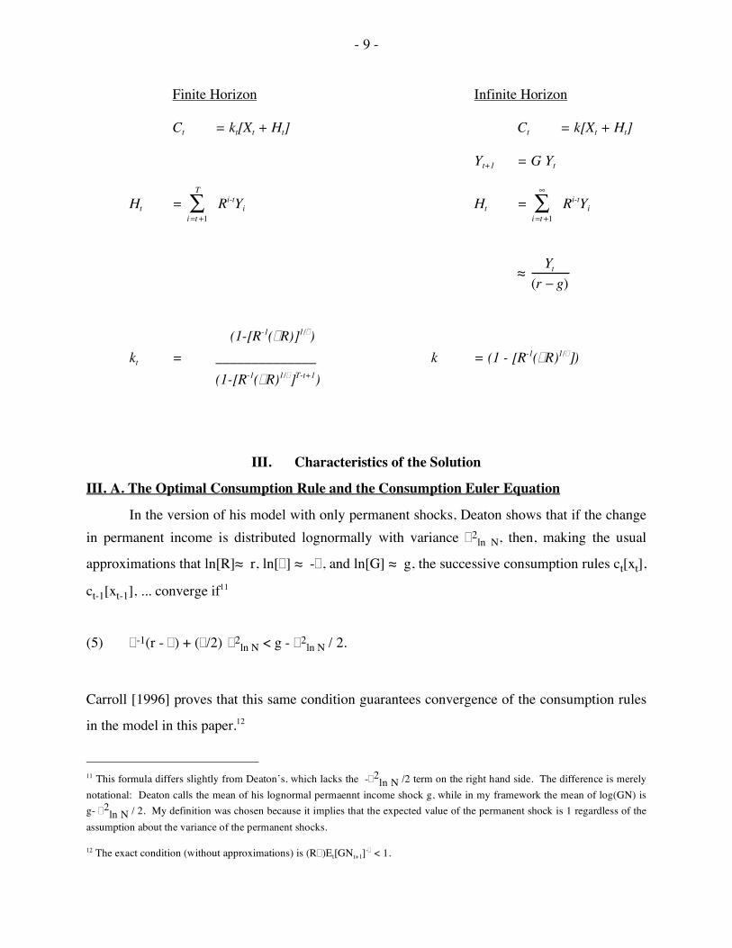
For purposes of comparison, a brief description is in order of the model I will refer to as

the “standard” model. The specific model I will consider is the perfect certainty version of the

CRRA model described above, i.e. the model that would apply if the transitory and permanent shocks were known in advance to always be equal to their expected values, Vt = Nt = 1 for all t,

although results in most cases would be very similar for the version of the model with quadratic

utility and uncertainty. Defining human wealth H as the present discounted value of the expected

stream of future income, and denoting the marginal propensity to consume by k, the solution to

this model in the finite and the infinite horizons is given by:

10 They refuse to borrow essentially for precautionary reasons, fearing the consequences of borrowing and then earning zero income indefinitely, so that eventually consumption is driven to zero. The no-borrowing result is less special than it may appear, however; the qualitative characteristics of the model are unchanged if the lower bound on income is positive. In that case, consumers will sometimes borrow, but will never borrow more than the present discounted value of the minimum possible future income stream. In effect, this amounts only to a shift in the horizontal axis for the problem. For a more detailed discussion, see Carroll [1992].

- 9 -

Finite Horizon Infinite Horizon Ct = kt[Xt + Ht] Ct = k[Xt + Ht] Yt+1 = G Yt

Ht = i=t +1

T

 Ri-tYi Ht = i=t +1

•

 Ri-tYi

≈ Yt

(r - g)

(1-[R-1( � R)]1/� ) kt = ______________ k = (1 - [R-1( � R)1/� ]) (1-[R-1( � R)1/� ]T-t+1)

III. Characteristics of the Solution

III. A. The Optimal Consumption Rule and the Consumption Euler Equation

In the version of his model with only permanent shocks, Deaton shows that if the change in permanent income is distributed lognormally with variance � 2

ln N, then, making the usual

approximations that ln[R]≈ r, ln[ � ] ≈ - � , and ln[G] ≈ g, the successive consumption rules ct[xt],

ct-1[xt-1], ... converge if11

(5) � -1(r - � ) + ( � /2) � 2

ln N < g - � 2ln N / 2.

Carroll [1996] proves that this same condition guarantees convergence of the consumption rules

in the model in this paper.12

11 This formula differs slightly from Deaton’s, which lacks the -� 2

ln N /2 term on the right hand side. The difference is merely notational: Deaton calls the mean of his lognormal permaennt income shock g, while in my framework the mean of log(GN) is g- � 2

ln N / 2. My definition was chosen because it implies that the expected value of the permanent shock is 1 regardless of the assumption about the variance of the permanent shocks. 12 The exact condition (without approximations) is (R � )Et[GNt+1]-� < 1.

- 10 -

The intuition for this equation is easiest to grasp if we assume � 2ln N = 0 momentarily. In

the standard model, the growth rate of consumption is � -1(r - � ).13 Now consider a consumer

with zero assets. Because the PDV of income must equal the PDV of consumption, if

consumption growth will be slower than income growth over the remainder of the lifetime (i.e. if

(5) holds), the level of consumption today must be higher than the level of income today. Thus,

the condition boils down to whether the consumer is sufficiently impatient that he would wish to

dissave (or borrow) today to finance current consumption, if future income were perfectly certain. The more general case, with the � 2

ln N/2 terms reflects, on the left hand side of equation

(5), the additional consumption growth induced by the permanent income shocks, and, on the

right hand side of the equation, the reduction in the mean growth of the log of income necessary to maintain EtNt+1 = 1 (without this adjustment EtNt+1 would increase with � 2

ln N). Equation (5)

is the condition referred to informally in the introduction as the “impatience” assumption,

although note that this equation can be satisfied by consumers who do not discount future utility at all ( � = 0) but who face positive income growth.

Many of the important results from the buffer-stock model can be understood by

considering the log-linearized consumption Euler equation, which takes the form

(6) Et � ln Ct+1 ≈ � -1(r - � ) + ( � / 2) vart ( � ln Ct+1) + et+1

if shocks to consumption are lognormally distributed.14 The bulk of previous work on

consumption (see, e.g., Hansen and Singleton [1983], Hall [1988], Zeldes [1989b], Lawrance

[1991]) has essentially ignored the expected variance term in the consumption Euler equation,

assuming it to be either a constant or zero.

13 Again, this is an approximation. The exact result is that (ct+1/ct)=(R � )-1/� . Henceforth, in the text and in figures, I will approximate log (R � ) with (r-� ) and log G with g without further comment, although in all the calculations the correct (not approximate) formulae are used. 14 See, e.g., Deaton [1992]. If shocks to consumption are not lognormally distributed, a similar equation can be derived using a Taylor expansion of the Euler equation, see Dynan [1993]. The formula in equation (6) was used because it is more intuitive than the expression from the Taylor expansion.

- 11 -

Figure Ia summarizes many of the important features of the buffer-stock model. The curve labelled “� (x) = Et � ln Ct+1” corresponds to the expectation of consumption growth

(calculated numerically using the converged consumption rule) as a function of the consumer’s gross wealth-to-income ratio. The horizontal line drawn at � � 1(r - � ) indicates the growth rate of

consumption that would prevail in a standard model with CRRA utility and baseline parameter

values but with no labor income uncertainty.15 The other horizontal line is the expected growth rate of permanent income, g’ = Et � ln Pt+1 = g - � 2

ln N /2, which under these parameter values is

greater than � � 1(r - � ) - �� 2ln N/2, thus guaranteeing that these consumers are “impatient” in the

required sense of equation (5). The vertical line labelled “x*” represents the target value of the gross wealth ratio, i.e. x* is the xt such that Et xt+1 = xt.

The first point the figure illustrates is the inadequacy of the common assumption that the variance of consumption growth is constant or zero: The gap between the Et � ln Ct+1 curve and

the � � 1(r - � ) line is strongly declining in the level of the gross wealth ratio.16 This happens for

the intuitive reason that consumers with less wealth have less ability to buffer their consumption

against shocks to income. More formally, the declining variance is a result of the fact that the

optimal consumption rule is strictly concave; in other words, the marginal propensity to consume

is a strictly decreasing function of the level of wealth. (Carroll and Kimball [1996] prove the

strict concavity of the consumption function for a wide class of problems which includes this

one). The link between concavity and the variance term stems from the fact that at low levels of

wealth, the marginal propensity to consume is high, so for a poor consumer a given amount of

variation in income will induce a larger amount of variation in consumption than the same

income variation would induce for a consumer with more wealth and thus a lower MPC. Carroll [1996] formally proves a variety of propositions about this figure. First, as xt � 0,

15 In fact, the CRRA model with certain income does not have a well-defined solution for the baseline income growth and interest rate parameter values, because with an interest rate less than the income growth rate, the present discounted value of future income is unbounded. However, for a finite-horizon version of the certainty model where the horizon is arbitrarily long, it remains true that the growth rate of consumption will be given by � � 1(r - � ). 16 Strictly speaking, the gap between � (x) and � � 1(r-� ) is not exactly proportional to the variance of expected consumption growth, because equation (6) is an approximation. Qualitative statements about the gap and the variance are interchangable, however, so as a heuristic tool I will speak of the gap interchangably with the variance.

- 12 -

the expected rate of consumption growth goes to infinity (although for graphing purposes the expected consumption growth locus is truncated at 10 percent). This is essentially because as xt

� 0, Ct � 0 and therefore log Ct� -∞. Second, as xt � ∞, the expected growth rate of consumption

approaches � � 1(r - � ), the growth rate that prevails in the perfect certainty model. This is because

as wealth approaches infinity, the proportion of future consumption the consumer expects to

finance out of his (uncertain) labor income becomes infinitesimal, so for all practical purposes

labor income uncertainty becomes irrelevant.17 Third, there exists a target wealth-to-income ratio x* such that if xt = x*, Etxt+1 = x*, and that target is “stable” in the sense that if xt > x*,

Etxt+1 < xt and vice versa. (This result justifies the directional arrows on the expected

consumption growth locus.)

The fourth proposition is a correction of a proposition in Carroll [1992]. That paper

argued that at the target gross wealth ratio x*, expected consumption growth was

“approximately” equal to expected permanent income growth,

Et [ � ln Ct+1 | xt = x*] ≈ Et � ln Pt+1.

Carroll [1996] shows that a more appropriate approximation is

(7) Et [ � ln Ct+1 | xt = x*] ≈ Et � ln Pt+1 + � ’’[x*] Et

(xt+1

- x*)2

2

where � [x] = log c[x].18 Carroll [1996] uses the proof in Carroll and Kimball [1996] of the strict

concavity of the consumption function to show that the � ’’[x*] term is strictly negative. Thus,

expected consumption growth for consumers holding x* is strictly less than the expected growth

rate of permanent labor income. This is visible in the figure from the gap between the

17 This proof requires an additional restriction on parameter values, g < r, which is not satisfied by my baseline parameter values but is satisfied by some of the alternative parameter values considered later. 18 The intuition here is Jensen’s inequality: because the expected growth curve is convex, the average growth of consumption for consumers distributed around the target wealth will be greater than the expected growth rate at the target.

- 13 -

intersection of the x* line with the Et [ � ln Ct+1] locus and the intersection of the x* line with the

Et [ � ln Pt+1] line.

Figure Ib provides an example of how to perform experiments with the figure. The solid

lines represent a blowup of the middle portion of figure Ia, while the dashing lines show how the

figure changes if g, the expected growth rate of labor income, declines from the baseline value of

g=.02 to a new value of g=.005 annually. (The dashing horizontal line indicates the new, lower expected income growth rate, g2’ = g2 - � 2

ln N /2 = .005 - .005 = 0). Even though the expected

income growth rate does not appear directly in the Euler equation for consumption growth (6),

the locus depicting the expected growth rate of consumption does shift, from its original position � 1(x) to � 2(x), the downward-sloping dashing curve. The expected consumption growth curve

shifts because the expected variance term in (6) at a given x changes; the new optimal

consumption rule will differ from the old one, so at a given x the same amount of variation in

income can produce a different amount of variation in consumption. The new target wealth ratio

x*2 is greater than the original one; thus, as one would suspect, when consumers expect slower

income growth, they hold more wealth. This is the manifestation of the “human wealth effect” in

this model. The new � 2(x) locus in Figure Ib was constructed by solving the whole model under the

new growth rate assumption and again numerically calculating the expectation of consumption

growth as a function of x. It would be convenient if there were a shortcut to this laborious

process, but unfortunately there appears to be no other way to obtain accurate quantitative

answers to questions about how target wealth changes when parameter values change. On the

other hand, there is a simple procedure which appears always to give correct qualitative answers to such questions. Define � [x*] = [Et � ln Ct+1 | x = x*] - Et � ln Pt+1; that is, � corresponds to the

last term in equation (7), the gap between expected consumption growth and expected income

growth for a consumer with wealth equal to target wealth. Now, to determine how a given

parameter affects target wealth, shift only the curves which directly reflect the parameter in question, and find the value of x* which leaves � [x] the same as under the original parameter

values. Figure Ic illustrates how this procedure would apply to the experiment that is performed

“correctly” in figure Ib, a decline in the expected growth rate of income. Because the only locus

- 14 -

that directly reflects the growth rate is the growth curve itself, that is the only curve in the figure that needs to be shifted. The new x*, x*’

2, is drawn at the point that leaves the gap � between Et

[ � ln Ct+1 | x = x*] and Et � ln Pt+1 unchanged. As with the “correct” procedure in Figure Ib, the

qualitative answer this exercise yields is that a decline in the growth rate of income produces an

increase in the target wealth ratio.

III. B. The Steady-State Distribution of Assets

The description of the implications of the model thus far has focused on features and

implications of the optimal consumption rule. This is in keeping with most previous research,

including Zeldes [1989a] and Kimball [1990a], who, for instance, examine the effect of

uncertainty on the marginal propensity to consume at given levels of wealth or consumption, but

do not examine what levels of wealth and consumption will prevail. As a result, the main

implications they are able to draw about the differences between their models and standard

models are qualitative - for their models, the marginal propensity to consume out of transitory

income will be higher, consumers will hold more wealth, the expected growth rate of

consumption will be greater, than for the standard model. However, to compare the model to

quantitative empirical results, it is necessary to be able to answer the question how much greater

will the MPC be, on average? How much higher is wealth, typically? How much faster is

consumption growth, on average? And how do the answers to these questions depend on

assumptions about the degree of income uncertainty, the value of taste parameters, and the

expected growth rate of income?

To answer such questions it is necessary to compute the distribution of wealth implied by

the model. Presumably one reason Zeldes did not attempt this is that in a finite-horizon version

of the model, the consumption rules and the distribution of wealth change in every period of life,

so the answers to those questions would have been different for every period of life. It would be

difficult, therefore, to summarize the results.

Things are potentially much simpler in the infinite-horizon context. Clarida [1987]

showed that in a similar model with liquidity constraints, no permanent shocks, and no growth,

the distribution of assets will be ergodic, converging toward a fixed “steady-state” distribution. If the permanent shocks in this model are removed (i.e. Ni,t=1 for all t), this model satisfies the

- 15 -

critical condition for ergodicity posed in Clarida [1987] (see Carroll [1996] for a proof).

Unfortunately, I have been unable to construct a general proof of ergodicity for the model with

permanent shocks. Nonetheless, for any particular converged consumption rule, if an ergodic

distribution exists, it can be found by numerical methods. (See Appendix II for a description of

the numerical procedure).

Figure II shows the evolution of the distribution of the net wealth ratio over time in a

simulated economy containing 20,000 households who all behave in every period according to

the converged consumption rule derived under the baseline parameter values. Consumers in the simulation begin life with zero assets and permanent labor income in the first period of Pi,1 = 1

for every household i. In each subsequent period of life, each household receives independent

shocks drawn from the income distributions described above.19 What is depicted in Figure II is

the temporal evolution of the across-household distribution of the net wealth ratio, where net

wealth is defined as the remaining wealth in a period after the household has drawn all shocks

and has consumed the desired amount. (This concept corresponds better to the data typically

reported in wealth surveys than does the gross wealth ratio x used heretofore in this paper.)

Convergence of the distribution toward the steady state distribution is rapid. From a

starting value of zero, after only three periods of life the mean net wealth ratio is 0.27, compared

to an estimated steady-state value of 0.34. The speed of convergence to the steady-state is

interesting because if convergence is rapid, it is more likely that any steady-state results derived

will also apply, at least roughly, to collections of consumers out of steady-state.

III. C. The Relationship Between Consumption Growth and Income Growth

Table I presents some summary statistics about the “steady-state” behavior of collections

of buffer-stock consumers who all have identical preferences. Each row presents results when

all parameters are at their baseline values except the parameter designated in the first column,

which takes the indicated value. The most striking result is shown in Columns 2, 3, and 4: the

expected growth rate of households’ consumption always matches the expected growth rate of

their permanent labor income, and the growth rate of their aggregate consumption always

19 I assume that there are no aggregate shocks.

- 16 -

matches the growth rate of their aggregate labor income. This section explains how these results

arise.

Consider a collection of ex ante identical buffer-stock consumers indexed by i who as of period t have achieved among them the steady-state distribution for ci,t, the ratio of consumption

to permanent income. Designating E.,t as the expectation taken across all households as of time

t, the average expected growth rate of consumption for these consumers is given by:

(8) E.,t � ln Ci,t+1 = E.,t [ ln Ci,t+1 - ln Ci,t]

= E.,t [ ln ci,t+1GNi,t+1Pi,t- ln ci,tPi,t]

= E.,t [ ln GNi,t+1 + ln ci,t+1 - ln ci,t]

= E.,t [ ln GNi,t+1] + E.,t [ln ci,t+1] - E.,t [ln ci,t] = E.,t [ ln GNi,t+1] = g - � 2

ln N/2,

where the last equality follows because in steady-state the average value of the consumption ratio does not change from one period to the next, E.,t [ln ci,t+1] = E.,t [ln ci,t].

In the same notation, equation (6) can be rewritten as:

(6’) E.,t � ln Ci,t+1 ≈ � -1(r - � ) + ( � /2) E.,t var ( � ln Ci,t+1).

We now have two expressions, equations (8) and (6’), for the expected growth rate of

consumption, taking expectations across consumers at a point in time. The two equations share a

single endogenous variable, the expected variance of consumption growth. Obviously this

means we can solve for the endogenous value of the expected variance:

(9) E.,t [ var i,t( � ln Ci,t+1) ] ≈ (2/ � ) [g - � 2

ln N/2 - � � 1(r - � )].

Of course, as Figure I vividly illustrates, the variance of consumption growth is also a

negative function of the level of wealth. Using that fact in conjunction with equation (9) yields

intuitive predictions. For example, at higher interest rates the right hand side of equation (9) will

- 17 -

be smaller, corresponding to a smaller average consumption variance and thus a higher average

level of wealth; in other words, the interest elasticity of average wealth is positive.20 Similar logic can be used to show that wealth is higher for consumers who discount the future less ( �

falls) or for consumers with lower expected permanent income growth (the human wealth effect). The coefficient of relative risk aversion has offsetting effects: A higher � represents a stronger

precautionary saving motive (reflected in the 2/ � term), and on its own would increase average

wealth. But a higher � also corresponds to a lower intertemporal elasticity of substitution

(reflected in the � � 1 (r - � ) term), which should result in lower wealth if consumers are impatient.

The overall effect of � on wealth is therefore ambiguous.

Because the average growth rate is not the same as the growth rate of the average, the above proof that E.,t � ln Ci,t+1 = E.,t � ln Pi,t+1 does not prove that � ln E.,t Ci,t+1 = � ln E.,t Pi,t+1.

Yet Table I showed that in the simulations both propositions held true. It is surprisingly difficult

to prove that the average growth rate of aggregate consumption is equal to the average growth

rate of aggregate income in the buffer-stock model. Because the proof is difficult but not

enlightening it is not presented here; interested readers can find it in Carroll [1996].

A word is in order about the subtle but important difference between the kind of analysis

contained in the previous section and embodied in Figure I, and the kind of analysis just

presented that can be done using equations (6’) and (9). Figure I and its discussion reflected only

statements about the optimal behavior of an individual consumer; nowhere were implications

about aggregates or averages across consumers derived or discussed. On the other hand, the

logic used to obtain equation (9) relied critically on an assumption that there was a population of

consumers across whom the distribution of consumption (and other variables) had reached its

ergodic steady-state.

20 The reasoning relating parameter values to mean wealth in this sentence and the rest of the paragraph cannot be formally justified, for several reasons. For example, the demonstration in Figure I that vart (� ln Ct+1) is a negative function of xt does not absolutely guarantee that when the equilibrium variance falls mean wealth must rise. That would only follow with absolute necessity if the new steady-state distribution of x were identical to the original distribution except for a location parameter, and if the relationship between vart (� ln Ct+1) and xt were linear, neither of which is true. Furthermore, even equation (9) itself relies on approximations. Equation (9), and the methods for reasoning about average wealth from it, should be viewed as a heuristic tool rather than a rigorous analytical framework. That said, I have found no parameter values for which this kind of reasoning from equation (9) gives the wrong answer.

- 18 -

III. D. Implications for Empirical Research

The most important implication of equation (9) is that typical methods of Euler equation

estimation, on either household or aggregate data, yield meaningless results if the consumers

involved are buffer-stock savers, because typical methods assume that the variance term in the

Euler equation is either zero or a constant. This subsection illuminates the potential pitfalls for

Euler equation estimation using examples, first from the literature on Euler equation estimation

with household data and then from the literature on aggregate Euler equation estimation.

Lawrance [1991] estimates consumption Euler equations across households of different

educational levels, assuming a constant value of the variance term across households.

Simplifying considerably, she finds that consumption growth is faster for households with

greater education, and concludes that education must be correlated with the pure rate of time preference, � . However, a large literature in labor economics has established that households

with greater education have faster labor income growth. The dependence of consumption growth on income growth in the bufer-stock model strongly suggests that Lawrance’s estimates of �

might simply be proxying for the effects on consumption growth of predictable differences in

income growth.

Because the issues here are both subtle and important, it is vital to be perfectly clear

about the nature of the problem. A simple example will illustrate how results like Lawrence’s

could arise in a buffer-stock framework despite identical time preference rates across

households. Suppose that the population consists of two kinds of consumers, H and L, identical

in every respect (including taste parameters) except that the mean growth rate of permanent labor income is higher for consumers in group H than for consumers in group L, gH > gL. Suppose

further that the two groups of consumers have respectively converged to their steady-state wealth

distributions. Now imagine estimating an equation of the form: � ln Ci,t+1 = � 0 + � 1 Ei,t ri,t+1 + � 1 Di + � i,t+1

across this whole population of consumers, with the dummy variable D equal to one for consumers of type H and 0 for consumers of type L. The estimated coefficient on Dii will be (gH

- 19 -

- gL), as can be seen by plugging equation (9) with different growth rates into equation (6’). The

Lawrence interpretation of this finding would be that consumers in group H have a lower

discount rate than consumers in group L, even though by assumption the data were generated by

consumers with identical time preference rates. The problem is in the omission from the

estimating equation of the endogenous variance term, which buffer-stock theory indicates ought

to be correlated with Dii.. In econometric terms, this is an omitted variable problem, where the

omitted variable is correlated with the included variable D.

Even papers which explicitly acknowledge the presence and potential non-constancy of

the variance term face substantial problems. One of the earliest and best of these papers is

Dynan [1993]. She uses data from the Bureau of Labor Statistics’ Consumer Expenditure

Surveys to calculate consumption growth rates and variances of consumption growth rates for

different groups of households and estimates an equation of the form

� ln Ci,t+1 = � 0 + � 1 Ei,t ri,t+1 + � 2 E.,t var( � ln Ci,t+1) + � i,t+1

by instrumental variables, using as instruments the head of household’s education, occupation,

age, and a variety of other characteristics. She finds a coefficient close to zero on both the Ei,t ri,t+1 term and the E.,t var( � ln Ci,t+1) term.21 Dynan considers herself to be estimating equation

(6) and thus expects the coefficient on r.,t+1 to equal � -1 and the coefficient on E.,t var( � ln Ci,t+1)

to be ( � /2). A coefficient estimate of zero for � 1 would therefore imply a coefficient of relative

risk aversion of � = ∞, while a coefficient of zero on the variance term implies � = 0. However,

Dynan focuses on the coefficient estimate for E.,t var( � ln Ci,t+1), and concludes that her data

provide no evidence for the existence of a precautionary saving motive (a precautionary motive requires a strictly positive � ).

If Dynan’s consumers were engaged in buffer-stock saving, however, coefficient

21 An important subtlety: for simplicity, I will assume that Dynan’s instruments are effectively isolating separate groups of consumers with different group characteristics. In this case the E.,t notation represents the instrumented value of the variable whose expectation is being taken.

- 20 -

estimates of zero on both these terms would be unsurprising. The simplest example of how such

a result could arise is as follows. Consider a sample which contains households that fall into

several groups identifiable to the econometrician via instruments like Dynan’s (education groups,

say). Suppose that the households in the groups are identical in every respect except for the

interest rates they face and their rates of time preference. In the buffer-stock framework, on

average the impatient groups of consumers will end up holding less wealth. Their smaller

buffer-stocks reduce their ability to shield consumption against income shocks, resulting in a larger value for

r

2 E.,t var( � ln Ci,t+1). Under these circumstances, group membership would be

highly statistically significant (as Dynan’s instruments are) in a first-stage regression of the

variance term and the interest rate term on group dummies, yet all consumers would end up with

the same growth rate of consumption (their shared growth rate of income g) despite having predictably different values of both E.,t var ( � ln Ci,t+1) and E.,t ri,t+1. The regression’s intercept

term � 0 would be estimated to equal g and the coefficients on the interest rate and variance terms

would both be estimated at zero, as Dynan found. Similar logic holds if the coefficient of relative risk aversion varies across groups; the coefficient estimates for � 1 and � 2 would again be

zero. Taken as a whole, therefore, Dynan’s findings are actually supportive of a buffer-stock

model of precautionary saving, but only because, in contrast to the standard model, the buffer-

stock model is capable of explaining how both of her coefficient estimates could be estimated at

zero even if consumers in fact have a strong precautionary saving motive.

In principle, it is possible to estimate consumption Euler equations consistently across

groups of buffer-stock consumers, but the conditions required are quite stringent. In particular, it

is essential to have important and predictable differences across groups of consumers in both

interest rates and income growth rates, and no differences at all in tastes across groups. Without

variation in income growth rates, equation (9) indicates that the variance term and the interest

rate term should be perfectly collinear, preventing accurate coefficient estimation on either term.

Without variation in interest rates across groups, it is obviously not possible to estimate a

coefficient on the interest rate term.

The implications of this discussion for the estimation of consumption Euler equations

across households are thus rather grim, at least for groups of consumers who satisfy the

impatience condition (5). One might hope that the traditional Euler equation estimation methods

- 21 -

would at least be applicable to patient consumers who do not satisfy (5). Unfortunately,

however, even for finite-horizon patient consumers the variance term in the Euler equation will

be a declining function of wealth, because the proof of the concavity of the consumption function

in Carroll and Kimball [1996] holds regardless of taste parameters. Because the amount of

wealth accumulation accomplished by a given age, and therefore the variance term in the Euler

equation, depends on the time preference rate, the time preference rate cannot itself be estimated

consistently using Euler equation methods across such groups of consumers. Similar logic

applies to the coefficient of relative risk aversion. Of course, as the level of the gross wealth

ratio gets very large, the variance of consumption growth approaches zero and these problems

disappear. In fact, the only consumers for whom it is absolutely clear that taste parameters can

be consistently estimated via traditional consumption Euler equation methods are consumers

who possess effectively infinite wealth.

The message of the buffer-stock model for the estimation of household taste parameters

is not entirely nihilistic, however. Equation (9) itself can be estimated, most easily by regressing

group variances of consumption growth on group income growth rates and group-specific interest rates: this yields a direct estimate of (2/ � ) and therefore of � itself, assuming a � that is

constant across groups. One advantage of estimating (9) over direct estimation of the

consumption Euler equation is that consistent estimation of (9) need not require identical time

preference rates across groups. Indeed, if good instruments can be found for the growth rate of

income and for the interest rate, it should even be possible to use nonlinear methods to estimate

group time preference rates from equation (9).

A second, cruder test of the foundations of the buffer-stock model, and indeed of the

more fundamental property of the concavity of the consumption function, is suggested by Figure

I: simply examine whether the variance of consumption growth is higher for consumers with

lower wealth-to-permanent-income ratios. Perhaps the best empirical test along these lines

would be to look for consumers who experienced a major recent drop in their wealth (possibly

owing to a spell of unemployment), and to calculate the effects on the variance term and on

subsequent consumption growth.

Equation (9) and Figure I do not exhaust the empirical implications of the model for

household data. See Section V. for a brief discussion of a variety of recent empirical work which

- 22 -

matches the model to data in new ways that have little to do with Euler equation estimation.

Implications of the buffer-stock model for estimation of aggregate Euler equations are

similar to those for estimation across groups of households. If the population is normalized at 1, the aggregate and average levels of consumption will be the same; designate both as E.,t+1 Ci,t =

C.,t. In that case the relationship between aggregate labor income growth g and aggregate

consumption growth in the “steady-state” can be written simply as:

(10) � ln C.,t+1 = g.

The mechanism by which the growth rate of aggregate consumption converges to the

growth rate of aggregate labor income is essentially the same as that which caused expected

household consumption growth within groups of buffer-stock consumers to converge to expected

household income growth: Through the mediation of the endogenous variance term.

Households living in a more impatient country will have a lower value of household wealth, on

average, and therefore higher consumption variance, which will boost their consumption growth

enough to make consumption growth match income growth.

The model’s prediction that aggregate consumption growth should approximately equal

aggregate permanent labor income growth, at least in steady-state, may have the potential to help

explain many empirical failures of the standard Euler equation framework estimated using

aggregate data. The most obvious application is to the consumption/income parallel that Carroll

and Summers [1991] documented for cross-country aggregate data over periods of three to five

years and longer. Of course, standard growth models also predict that, in steady-state, income

growth and consumption growth will be “balanced.” The distinction between this model and the

standard model is that the transition to the steady-state is much faster here: Under baseline

parameter values, the transition half-life in the buffer-stock model is generally about two years;

in contrast, under standard parameter values the transition half-life in a Solow or Cass-

Koopmans growth model is on the order of fifteen or twenty years, and some authors (Mankiw,

Romer, and Weil [1992] in particular) favor parameter values that generate a half-life that is even

longer. The slow rate of convergence in the standard model was a primary reason Carroll and

- 23 -

Summers [1991] rejected the idea that the consumption/income parallel evident over periods of 3

to 5 years was a reflection of balanced growth steady-states.

Another piece of evidence Carroll and Summers [1991] mustered against the Cass-

Koopmans growth model as a description of aggregate consumption was that there is no apparent

relationship across countries between the average growth rate of aggregate consumption and

average country-specific interest rates. This result is easily explained in a buffer-stock

framework as resulting from the endogeneity of the variance term, which is not observed in

aggregate data and is hence inevitably omitted from aggregate Euler equation estimation.22 As

equation (9) indicates, the omitted variance term is in theory negatively correlated with the

interest rate. In fact, equation (10) summarizes all the implications of the buffer-stock model for

the steady-state relationship between consumption growth and interest rates, tastes, income

uncertainty, and other variables: the coefficients on all such variables should be zero when the

consumption variance term is omitted from the estimating equation.

The model may also help to shed some light on the findings of Campbell and Mankiw

[1989], who estimated an equation of the form: � ln Ct+1 = � 0 + � 1 Et rt+1 + � Et � ln Yt+1 + � t+1

where Et � ln Yt+1 was calculated using lagged variables that, according to traditional Euler

equation analysis, should be uncorrelated with current consumption growth. They found a highly significant estimate of � in the vicinity of .5. Their interpretation was that half of

consumption is done by consumers who set consumption equal to income, while the rest is done

by consumers who obey the standard Euler equation (although they did not find robust evidence

of a positive coefficient on the interest rate as would be expected for the consumers who

putatively obey the standard Euler equation).

Suppose that in the postwar period aggregate labor income grew according to

22 It is important to recognize here that the right variable is the variance of consumption growth at the microeconomic level. The omitted variance term therefore cannot be recovered from any kind of ARCH or GARCH estimation using aggregate data; it must be calculated using household level data, if at all.

- 24 -

� ln Yt = gt + et

where g represents the underlying rate of labor income growth and e represents transitory shocks to income growth. Furthermore, suppose gt = g1 for t before 1973 and gt = g2 < g1 for t after

1973, reflecting the productivity growth slowdown in the post-1973 period. Now suppose that

some subset of Campbell and Mankiw’s instruments also experienced a regime shift in the post-

1973 period, and therefore instruments dated t will do a good job indicating whether the

economy is in the slow-growth or fast-growth regime; finally, suppose another subset of instruments is highly correlated with et+1. The second-stage equation that Campbell and Mankiw

estimate is then in effect:

� ln Ct+1 = � 0 + � 1 Et rt+1 + � (gt+1 + e t+1) + � t+1

where gt+1 reflects the correlation of their instruments rates with underlying “permanent” growth

rate regime, and e t+1 reflects the correlation of their instruments with the predictable component

of transitory income growth. The buffer-stock model implies that, across steady-states, the coefficient on gt+1 should be one. It is less clear what the model would imply about the

coefficient on e, although the MPC out of transitory income should be an upper bound on the

coefficient on e. Although it is not clear what the coefficient on g would be during the transition

period between the pre-1973 and post-1973 growth regimes, the relatively rapid convergence of

the buffer-stock model under baseline parameter values suggests that this transition period would not last long, so the estimated coefficient on gt+1 should be close to one if separate coefficients

on g and e were estimated. However, when the two terms are combined into a single term for

predictable income growth, as Campbell and Mankiw do, any coefficient estimate between one

and the coefficient on e could be consistent with a buffer-stock model, depending on, among

other factors, the degree of correlation of the various instruments with the transitory and

permanent components of growth.

Whether in practice a buffer-stock model predicts something like the 0.5 coefficient that

- 25 -

Campbell and Mankiw typically found would depend in detail on the exact specification of the

model; setting up and solving such a model is well beyond the scope of this paper (although it is

an inviting project for future work). The argument here is only that a buffer-stock model at least

has the potential to explain Campbell and Mankiw’s results without assuming the existence of

consumers who blindly set consumption equal to income in every period.

One important caveat in using the model to explain aggregate data is that, even if the

typical household is a buffer-stock consumer, it is clear that at least some consumers do not

behave according to a buffer-stock model (see the discussion of very wealthy households in

section IVC). To the extent that aggregate consumption reflects the behavior of these non-

buffer-stock consumers, the buffer-stock model may not be able to match aggregate data even if

it is the right model for most consumers.

III. E. Other Implications

The results in Table I summarize other interesting characteristics of the steady-state

solution of the buffer-stock model under a variety of parameter values.

First, the Marginal Propensity to Consume. The standard model under baseline

parameter values implies an MPC out of transitory income of 2 percent. No commonly used set

of parameter values in the standard model implies an MPC of greater than about 8 percent (the

formula for the MPC in the standard models is given in Section II.C.). Table I shows that, over

the entire range of parameter values considered in the table, the MPC is much greater than for the

standard model: The average MPC for buffer-stock consumers is always at least 15 percent, and

ranges up to 50 percent.

Another interesting question is what the model implies about the relationship between

expected income growth and the personal saving rate. If the steady-state average net wealth ratio

is w* at income growth rate g, then (if the interest rate is zero) the personal saving rate necessary

to make wealth grow at rate g (thus keeping the wealth/income ratio constant) is s ≈ g w*. If the

target wealth ratio w* were a constant, the model would obviously imply that s ≈ g w* is higher

when g is higher. However, w* is a negative function of g; the standard term for the effect of g

on consumption and saving decisions is the “human wealth effect.” In practice, for all parameter

values considered here the human wealth effect is vastly smaller than in the standard model, so

- 26 -

across steady-states the elasticity of the saving rate with respect to the growth rate of income is

positive.

In addition to its implications for the relationship between saving and growth, the drastic

diminution of the human wealth effect compared to the standard model is also an interesting

finding in itself. Several recent empirical tests can be interpreted as providing evidence that

current consumption is affected much less by expected future income than the standard LC/PIH

model implies. Campbell and Deaton [1989] calculate the implied effect on human wealth of an

innovation in current income, and find that consumption greatly ‘underresponds’ to innovations

in human wealth. Carroll [1994] projects mean future income for a panel of households and

finds no evidence that predictable future income growth affects current consumption at all.

Viard [1993] shows that a standard LC/PIH model implies that the post-1973 slowdown in

productivity growth in the U.S. should have sharply boosted saving rates; instead, saving rates

have fallen.

Is the MPC out of human wealth in a buffer-stock model consistent with these results?

Unfortunately, such a question is difficult to answer because, in contrast to the standard LC/PIH

model, in precautionary saving models the MPC out of future income depends on the current

level of physical wealth, the distribution of the future income, and the consumption rules

expected to prevail over the entire remainder of the consumer’s horizon. There is thus no

general way to answer the question of how responsive consumption is to human wealth, because

the answer will depend on the exact experiment. It is possible, however, to answer a specific

question, such as how consumption would respond to an increase in the expected growth rate of

income from 2 percent to 3 percent per year. Consider Figure III, which presents the converged

consumption rules for infinite-horizon versions of the buffer-stock model and the certainty

version of the LC/PIH model in the case where the real interest rate is four percent, expected

income growth is either two percent or three percent, and other parameters are at their baseline

values.23 The straight lines indicate the optimal consumption functions in the perfect certainty

case; the curved functions represent the converged buffer-stock consumption rules. The dashed

23 The deviation of the interest rate from the baseline value of zero is motivated by the fact that the present discounted value of future income in the certainty case is infinite, making nonsense of the model.

- 27 -

functions correspond to the g=.02 cases and the solid functions to the g=.03 cases. When the

growth rate of income increases from two to three percent, human wealth defined as the present

discounted value of expected future labor income doubles,24 boosting consumption substantially

at all levels of gross wealth in the standard model. In the buffer-stock model, however,

consumption rises far less: Prudent buffer-stock consumers refuse to spend much out of

expected higher future income, because that income just might not materialize.

The same point is made numerically by Table II. Under the chosen parameter values the

MPC out of human wealth in the standard model is 3.8 percent; in the buffer-stock model the

MPC rises with current assets but remains very small over the entire range. Although not

precisely zero, it is easily small enough to be consistent with empirical estimates like those in

Carroll [1994] that indicate that the MPC out of human wealth is close to zero.

Another way to measure the degree of responsiveness of current consumption to changes

in expected future income is to calculate an implicit interest rate at which expected future income

can be said to be “discounted” when the consumer decides how much of that future income to

spend today. Appendix III describes how such a measure can be calculated; the results are

presented in the column entitled “Implied Discount Rate for Future Income” in Table II. The

results are striking: at a gross wealth ratio of 0.2, the implied rate at which future income is

discounted is 13,981 percent! This result arises because a consumer with gross wealth of only

0.2 is already consuming almost every penny, and when expected future income goes up, this

consumer is unable to spend more than a tiny bit extra today.

Even at more moderate values of the gross wealth ratio, the implied discount rate is

remarkably large. In particular, the target gross wealth ratio in this model is around 1.6; the

future income discount rate at a gross wealth ratio of 1.6 is about 22 percent.

IV. Buffer-Stock Saving and the Life Cycle: Resolving Three Empirical Puzzles

This section of the paper makes a systematic argument that a version of the LC/PIH

model which implies that consumers engage in buffer-stock saving behavior over most of their

working lifetimes fits the essential facts about the behavior of the typical household’s

24 This can be seen from the formula for human wealth in the infinite-horizon case in Section II.C.: H = Y/(r-g). At r=.04, g=.02, H = 50 Y; at g=.03, H = 100 Y.

- 28 -

consumption, income, and wealth better than either the “standard” LC/PIH model, a Keynesian

alternative, or the hybrid of the Keynesian and standard LC/PIH models proposed by Campbell

and Mankiw [1989].25

The buffer-stock version of finite-horizon LC/PIH model will reflect the same baseline

parameter values under which buffer-stock saving behavior emerges in the infinite-horizon

context, but with a lifetime income process calibrated to actual US household age/income

profiles. The perfect-certainty finite-horizon model briefly described in Section II.C. is what I

will call the “standard” LC/PIH model, although similar results would be obtained with a model

with quadratic or Constant Absolute Risk Aversion utility. The Keynesian model will be taken to be a model of the form C = � 0 + � 1Y + u, where consumption has a positive intercept � 0 and

there is a constant marginal propensity to consume � 1 that is close to one (perhaps .9). The

Keynesian model has not been taken seriously since the work of Friedman and Modigliani in the

1950s; it is examined here principally as an aid to understanding the nature of the evidence. The

final model is the Campbell-Mankiw model which blends the standard LC/PIH and the

Keynesian models by assuming that half of income goes to standard LC/PIH consumers and half goes to Keynesian consumers with � 0 = 0 and � 1 = 1.

Table III summarizes some of the principal points made below. I will argue that only a

buffer-stock version of the LC/PIH model is consistent with the overall pattern of facts.

IV.A.The Consumption/Income Parallel in Low Frequency Data

Perhaps the most striking point of Carroll and Summers [1991] is made by Figure IV:

Across occupations, differences in age/income profiles are closely paralleled by differences in

age consumption profiles.26,27 The figure shows that consumption growth and income growth are

25 I do not consider a model with uncertain income and liquidity constraints, as in Deaton [1991], because I view that model and the model presented here as close substitutes. Most of the evidence that I find to be consistent with the buffer-stock model presented here would also be consistent with Deaton’s model. 26 Carroll and Summers [1991] and Carroll [1994] provide evidence that the profiles for different occupational groups remain relatively stable over time. 27 Unlike the figure in Carroll and Summers [1991], income and consumption in this figure were adjusted for aggregate productivity growth by adding 1.5 percent to the growth of both the income and the consumption profiles in each year. Without this adjustment for aggregate productivity growth, Carroll and Summers found that for all occupations income reached a peak in middle age and then began declining, rapidly in some cases.

- 29 -

very closely linked over periods of a few years or longer, a phenomenon we dubbed the

“consumption/income parallel.” This phenomenon is interesting because there is no explanation

for it in the unconstrained standard LC/PIH framework; in that model the pattern of consumption

growth is determined by tastes and is independent of the timing of income. Of course, the Keynesian model C = � 0 + � 1Y + u can easily explain the

consumption/income parallel if � 0 is small and � 1 is near one. Little of the evidence Carroll and

Summers marshalled for the low-frequency consumption/income parallel would rule out such an

explanation; however, evidence presented in the next section (along with a mountain of other

evidence originally presented in the 1940s and 1950s by Modigliani, Friedman and others) is

much less favorable to the Keynesian model. The Campbell-Mankiw model with � = .5 has trouble explaining the consumption/income

parallel because the parallel is simply too close. The ocular regression of consumption on

income in Figure IV suggests a coefficient near 1, not near 0.5; the regressions of Carroll [1994]

also suggest coefficients much nearer 1 than 0.5.

Can a plausibly parameterized buffer-stock version of the LC/PIH model explain the low

frequency consumption/income parallel? To answer this question I simulate a finite-horizon

version of the model using income profiles calibrated to roughly match those in Figure IV. From

Figure IV it is appears that in some occupations, such as Unskilled Labor, labor income tends to

stop growing relatively early in life, while for others, such as Managers, income tends to

continue growing until late middle age; for other occupations, such as Operatives, income grows

quickly until middle age, then slowly until retirement. For the simulations, I will consider three

age/income profiles roughly calibrated using the data for Unskilled Laborers, Operatives, and

Managers shown in Figure IV. Specifically, the Unskilled Labor profile income grows at 3

percent annually from ages 25 to 40, and is flat from age 40 to retirement at 65. For Operatives,

labor income grows at 2.5 percent per year from age 25 to age 50, and then at 1 percent per year

until retirement. Finally, for Managers income grows at 3 percent a year from ages 25 to 55, and

declines at 1 percent a year from 55 to 65. Post-retirement income for all three categories is

The productivity adjustment does not alter the principal conclusion Carroll and Summers [1991] drew from their figure (and from a variety of other evidence):

- 30 -

assumed to equal 70 percent of income in the last year of the working life, because empirical

estimates suggest that the sum of pension, social security, and other noncapital income after

retirement typically falls to roughly 70 percent of its preretirement level.

Solving the finite horizon version of the model by backwards recursion on (4) produces

optimal consumption rules for each period of life. Estimates of average consumption and

income were generated as for Figure II and Table I by randomly drawing income shocks

according to the assumed income distributions, for 1000 consumers who start life with zero

assets.28 (The behavior of asset holding over the life cycle is discussed below).

The results are shown in Figure V. A rough summary of the results of Figure V would be

that consumers engage in buffer-stock saving behavior, and so consumption growth closely

parallels income growth, until roughly age 45 or 50. Around that age consumers switch over to

doing a bit of retirement saving, which allows the income profile to rise a somewhat above the

consumption profile in the years immediately before retirement.

It worth noting here that Friedman himself would not necessarily have interpreted Figure

IV as evidence against his conception of the PIH. Indeed, he almost seems to anticipate it:

For any considerable group of consumers the ... transitory components tend to average out, so that if they alone accounted for the discrepancies between permanent and measured income, the mean measured income of the group would equal the mean permanent component, and the mean transitory component would be zero. ... ... It is tempting to interpret the permanent components as corresponding to average lifetime values and the transitory components as the difference between such lifetime values and the measured values in a specific time period. It would, however, be a serious mistake to accept such an interpretation... (pp. 22-23) The permanent income component is not to be regarded as expected lifetime earnings; it can itself be regarded as varying with age. It is to be interpreted as the mean income at any age regarded as permanent by the consumer unit in question, which in turn depends on its horizon and

28 The slight upward fillip to consumption in the last two or three years of life occurs as consumers spend down their precautionary assets when they realize that the amount of uncertainty remaining is small. This feature is an artifact of the unattractive assumption of a certain date of death, and therefore is not one of the implications of the model on which I wish to concentrate. If the model were modified to incorporate length-of-life uncertainty by adding a probability of death in each year, it could likely replicate the results in Hubbard, Skinner, Zeldes [1995] who find that consumption slopes downward throughout the entire retirement period.

- 31 -

foresightedness. 29 (p. 93) - Milton Friedman, A Theory of the Consumption Function

Friedman explains that the principal reason interpreting “permanent income” as “average

lifetime income” is a mistake is because such an interpretation prejudges the issue of the length

of the “horizon” over which consumers calculate permanent income. Friedman later clarifies

what he means by the “horizon” when he says that the typical household discounts future income

at a rate of 33 1/3 percent. Although discounting future income at a 33 1/3 percent rate is very

difficult to justify in the standard model, as Table II shows, in a buffer-stock model an apparent

“discount” rate of 33 1/3 percent is not at all difficult to obtain.

IV.B. The Consumption/Income Divergence in High Frequency Data

It might seem that the low-frequency parallel between consumption and income suggests that a simple Keynesian model with � 0 near zero and � 1 near one is a better model than the

comparatively complicated buffer-stock or standard LC/PIH models. The Keynesian model,

however, was abandoned in the 1950s for a number of good reasons, perhaps the most important

of which was the discrepancy between estimates of the model using long-term aggregate data, which found � 0 near zero and � 1 near one, and estimates using cross-section household surveys

of consumption and income, which found � 0 to be substantially positive and � 1 to be much less

than one.

Friedman’s [1957] famous resolution of this puzzle was one of the persuasive pieces of

evidence for the Permanent Income Hypothesis. He showed that if C = P + u and Y = P + v,

where P represents permanent income and Y represents observed income and u and v are stochastic, then a regression of C on Y would produce an estimated � 1 coefficient on observed

income of far less than one even if the MPC out of permanent income is one. The logic is

identical to the now-familiar errors-in-variables econometric problem in which the coefficient on

a variable measured with error is biased toward zero. To complete the case, Friedman argued

29 Another indication that Friedman regards mean income as good indicator of permanent income is his statement that upon retirement “permanent income” typically falls by about 25% because pension income is less than working income.

- 32 -

that the reason � 1 was estimated to be much nearer one when long-term aggregate income data

were used was because such long-term data are dominated by changes in permanent income.

Friedman [1957] noted that another implication of the model was that groups within the

population for whom the variance of transitory shocks to income is relatively greater should have

a lower estimated marginal propensity to consume out of total income; as confirmation, he

presented evidence that farmers and entrepreneurs had a lower MPC than other households.

A closely related implication of the model is that groups of consuemrs with a greater

variance of transitory shocks should on average exhibit a greater divergence between consumption and income. The simple Keynesian model with � 0 close to zero and � 1 near one

has no such implication. To see this, nest the two models by defining consumption as C = P + �

v + u, where � is the MPC out of transitory income v. If � = 0, this corresponds to the permanent

income model, and if � = 1 it corresponds to the Keynesian model with � 0 = 0 and � 1 = 1. Now

we have:

var(C/Y) = var( (P + � v+ u ) / (P + v) )

= var( (1 + � v/P + u/P ) / (1 + v/P) )

≈ var( (1 + � v/P + u/P ) (1 - v/P) )

= var( (1 + � v/P + u/P - v/P - � (v/P)2 - (v/P) (u/P) )

≈ var( ( � -1) (v/P) + (u/P) ),

where the first approximation holds when v/P is not too far from zero, and the second

approximation holds if (v/P)2 and (v/P)(u/P) are both close to zero, which will be true for

plausible estimates of the magnitude of transitory shocks to income and consumption.30

Assuming that the covariance between (v/P) and (u/P) is zero, this becomes

var(C/Y) ≈ var( ( � -1) (v/P) ) + var(u/P) )

30 The standard deviation of logarithmic transitory shocks to income, which can be identified here with e/p, is estimated in Carroll [1992] to be 10 percent annually; for a one standard-deviation shock, the error in the first approximation is given by comparing 1/1.1 ≈ .91 to .9. For the second approximation, if the standard deviation of consumption shocks is roughly the same size, both (e/p)2 and (e/p)(u/p) should be small enough to safely ignore.

- 33 -

(11) = ( � - 1)2 var(v/P) + var(u/P).

Thus the Keynesian model ( � = 1) implies that the variance of the consumption/income

ratio is unrelated to the variance of transitory shocks to income, while the PIH model ( � = 0)

implies that the variance of the consumption/income ratio moves one-for-one with the variance

of transitory shocks to income.31

Table IV presents estimates of the variance of the consumption/income ratio by

occupation group calculated from the 1960-1961 Consumer Expenditure Survey, along with

estimates of the variance of transitory shocks to labor income taken from Carroll and Samwick

[1995a].32,33 It is clear that there is a strong positive association between the two variances across

occupation groups. A simple linear regression using the data in this table yields

var(C/Y) = .651 var(v/P) - .0072

(.128) (.0059)

which implies a value for � , the MPC out of transitory income, of about 0.2. This estimate is

statistically significantly different from both zero and one at the five percent level of

significance.

These results constitute stronger evidence against the Keynesian model than against the

standard LC/PIH model, because the usual errors-in-variables logic shows that any measurement

error in the estimate of the variance of transitory income by occupation group would bias the

regression coefficient on the transitory variance toward zero, the value implied by the Keynesian

31 Although the simple Permanent Income model discussed here is not explicitly a finite-horizion model, similar results would apply for the standard finite-horizon model described in section II.C. 32 The data in both datasets are for consumers between the ages of 25 and 50 -- that is, consumers in the age range where I argue that the infinite-horizon version of the buffer-stock model is a good approximation to the behavior of finite-horizon consumers. 33 Carroll and Samwick [1995a] used essentially the same technique to decompose shocks to income into transitory and permanent components that Carroll [1992] and Hall and Mishkin [1982] used. This technique is unable to distinguish transitory shocks to income from white noise measurement error in income. However, the point of the table is not related to the level of the transitory variance, but rather to the differences in estimated transitory income across groups. If the variance of measurement error is the same across occupation groups, the coefficient on the regression (and the implied estimate of the MPC out of transitory income) is unbiased.

- 34 -

model. The coefficient is very significantly different from zero despite this bias toward zero, so

the rejection of the Keynesian model is even stronger than implied by the simple t-statistic.

The same bias, however, weakens the case the regression makes against the standard

LC/PIH model; it is conceivable that errors-in-variables bias is the only reason the MPC out of

transitory income was estimated to be 0.2 rather than zero. Of course, this regression is not the

only evidence that the MPC out of transitory income is too large to be consistent with the

standard LC/PIH model. Early tests of the permanent income hypothesis found that the marginal

propensity to consume out of unexpected, nonrecurring windfall payments was somewhere

between .15 and .5. (see, e.g., Bodkin [1959], Kreinin [1961], and the discussion by Mayer

[1972]).34 Similar results have been found by many subsequent authors proceeding through Hall

and Mishkin [1982] to very recent work by Nicholas Souleles [1995].35

Table I showed that the average MPC out of transitory income is 15 percent or greater in

the buffer-stock model for all combinations of parameter values considered in the table. Similar

MPCs arise over most of the working lifetime in the finite-horizon version of the buffer-stock

model; results are not reported to conserve space. Of course, other parameter values could

generate either larger or smaller MPC’s; the essential point is that the buffer-stock model has no

difficulty generating an MPC large enough to match even the larger empirical estimates, while,

for plausible parameter values, the standard LC/PIH model is simply incapable of implying large

values for the MPC out of transitory income.

It is again worth noting that Friedman would not have found these results inconsistent

with his understanding of the Permanent Income Hypothesis. Friedman [1963] states that the

Permanent Income Hypothesis implies a marginal propensity to consume out of purely transitory

income of about 0.3.

IV.C. The Behavior of Wealth Over the Lifetime

34 Two natural experiments were examined in these papers: in the U.S., the response of consumption to the “National Service Life Insurance Dividend of 1950,” a special payment to World War II veterans, and in Israel, reparations payments to victims of German persecution during World War II. The authors argue that both were unanticipated and transitory shocks to income. 35 Although they interpret their results as suggesting that 20 percent of consumption is done by consumers who set consumption equal to income, an alternative interpretation is that all consumers have a marginal propensity to consume out of transitory income of 20 percent.

- 35 -

Diamond and Hausman [1984] called attention to the fact that the median household

typically holds surprisingly small, but still positive, amounts of financial wealth over the entire

working lifetime. Table V illustrates this point using data from the 1963, 1983, and 1989

Surveys of Consumer Finances. In all three surveys, at all ages before retirement, the ratio of

median financial assets to median annual income is between 2 percent and 35 percent. In all

three surveys the ratio rises modestly from ages 25 to 55, and then rises sharply in the last decade

before the typical retirement age of 65.

The fact that the median ratio of wealth to income stays within a rather narrow range until

just before retirement is not necessarily inconsistent with the standard LC/PIH model. Indeed,

any particular pattern of wealth accumulation over the lifetime can be justified by some set of

assumptions about tastes and the pattern of income over the lifetime. The stability of the

Diamond-Hausman phenomenon between the early 1960s and the late 1980s, however, is

troubling for the standard LC/PIH model, because at some point between these two surveys there

was a sharp slowdown in productivity growth and expected future productivity growth [Viard,

1993].

To explore the implications of the standard and buffer-stock versions of the LC/PIH

model for the age profile of the wealth ratio, I solved both models for the age-income profile

labelled “Operatives” in Figure V, which was calibrated using the 1960s data. Under baseline

parameter values, the standard LC/PIH model implies large negative wealth holding over most of

the life cycle; however, there are obviously other parametric assumptions under which the model

implies positive wealth. I experimented with the assumed interest rate and found that an

assumed interest rate of eight percent per year produced the age/wealth profile that most closely

resembled the pattern in Table V. The result is the age-wealth profile labelled “Faster

Productivity Growth” in Figure VI. I then solved the model again assuming that the post-1973

productivity growth slowdown resulted in a one percent slower growth rate of labor income over

the working lifetime.36 The resulting age/wealth profile is labelled “Slower Productivity

Growth.” The difference between the two curves is a rough measure of how the productivity

36See Carroll and Summers [1991] for some evidence that this is a good approximation of reality.

- 36 -

slowdown should have affected the age/wealth profile for U.S. consumers if the standard LC/PIH

model were correct. The figure shows that lower growth should have induced an enormous

increase in household wealth at all ages greater than 30. On average, the “Slower” curve is

higher than the “Faster” curve by an amount equal to roughly two years’ worth of income.

Comparison to Table V indicates that the model’s predicted enormous increase in household

wealth/income ratios is more than an order of magnitude greater than the actual increase in

wealth/income ratios.

The results for the same experiment with the buffer-stock model are shown in Figure VII.

The profile of the wealth ratio over the lifetime in this figure bears a strong resemblance to the

profiles shown in Table V. Very early in life, the wealth ratio is low. For the middle two

decades it grows slightly, and then in the last decade before retirement the wealth ratio grows

sharply. The ratio is uniformly a bit higher in the economy with slow productivity growth, but

the difference between the two wealth profiles is not remotely so dramatic as in the standard

model. The implication of a slightly higher wealth ratio in the slow-growth equilibrium is

consistent with the pattern in Table V: for every age category, the wealth ratios are a bit higher

for the 1983 and 1989 surveys than for the 1963 survey.

Of course, the correspondence between the figure and the tables is not perfect. Under the

chosen parameter values, the buffer-stock model implies a considerably larger buffer-stock than

is evident in Table V. The model’s predictions could be brought more in line with the results in

Table V by assuming consumers are more impatient, or less risk averse, that they face less

uncertainty, or that they face a faster growth rate of income.

One objection to this line of argument might be that comparison to Table V is not

appropriate, because the standard LC/PIH model’s implications are about total net worth, not

about financial assets. However, similar calculations comparing the ratio of net worth to income

in the 1963, 1983, and 1989 survey produce similar conclusions: wealth-to-income ratios

increased only slightly from the 1960s to the 1980s, rather than by the enormous amounts the

standard model would imply.37

37 It would not be appropriate to include, say, expected future pension benefits in the measure of wealth. As shown in Table 2, in this model there is no single interest rate at which it is appropriate to discount uncertain expected future income.

- 37 -

One feature of the model that appears to be strongly at variance with available evidence

is its implication that wealth falls sharply after retirement, reaching zero in the year of death.

This implication is a result of the assumptions that the date of death is known with certainty, that

there is no bequest motive, and that forms of uncertainty other than labor income uncertainty

(such as uncertain medical expenses) do not intervene to boost the saving rate as consumers

age.38 Because it does not address these issues, the buffer-stock model is probably less useful in

understanding the behavior of the elderly than it is for describing the working population,

particularly the working population well before retirement age.

Less formal evidence about the reasons for holding wealth may also be illuminating. As

noted in the introduction, many more people cite “emergencies” than “retirement” as the most

important reason for saving. Another informal source of evidence about how people think about

uncertainty and savings is provided by personal financial planning guides. These guides

commonly have passages that suggest that consumers should maintain a buffer stock of assets

against uncertainty. The following is a typical passage:

It is generally held that your liquid assets should roughly equal four to six months' employment income. If you are in an unstable employment situation ... the amount should probably be greater. The Touche Ross Personal Financial Management and Investment Workbook, 1989, p. 10.

As both this quotation and intuition suggest, one of the implications of a buffer-stock

model is that consumers with higher income uncertainty should hold more wealth. Several

recent papers have found empirical evidence that precautionary saving is statistically significant

and economically important. Using wealth and income uncertainty data from the PSID, Carroll

and Samwick [1995a,b] find that wealth is substantially higher for consumers who face greater

income uncertainty. Carroll [1994] provides some evidence that consumers with more variable

incomes save more. Kazarosian [1990] finds, in a regression of wealth on demographic

38 The certain date of death accounts for the upward fillip in consumption in the last two or three years of life. As the certain end of life approaches, uncertainty about future income approaches zero, so remaining precautionary assets are spent.

- 38 -

characteristics and income variability, that the degree of income variability is overwhelmingly

significant.

One further category of evidence on household wealth accumulation patterns supports the

buffer-stock interpretation of the LC/PIH model. This is observation by Avery and Kennickell

[1989] that wealth holdings are extremely volatile, even over short periods. They first attempt to

explain the changes in consumers' wealth between 1983 and 1986 with a statistical life cycle

model, but the model performs poorly, explaining at most about 8 percent of the observed

changes in wealth. The reason for the failure is that in the standard life cycle model wealth

changes glacially, gradually accumulating or decumulating depending on life cycle stage, while

in the SCF data wealth appears to fluctuate vigorously, just as would be expected in a model

where the primary purpose of holding wealth is as a buffer against random shocks to income.

Even if the buffer-stock model provides a good description of the patterns of financial

asset accumulation of the typical household, it is nevertheless clear that it is not a complete

model of household wealth accumulation. For the typical household, housing equity constitutes

a larger fraction of total net worth than do financial assets, and the buffer-stock model, with its

single perfectly liquid, perfectly riskless asset, is a poor vehicle for understanding housing

investments. One interpretation of the strong correspondence between the buffer-stock model’s

implications and observed patterns of financial asset holding and consumption behavior is that

consumers separate the housing decision from other consumption-saving decisions. Once they

have bought a house and committed themselves to a fixed monthly mortgage payment, they may

subject the remaining “disposable” income stream to buffer-stock saving rules.

Finally, even as a model of financial asset holding, the buffer-stock model cannot be

considered a complete description of the behavior of all households. This is illustrated by two

related facts. First, if all consumers behaved according to a buffer-stock model under the

baseline parameter values assumed here, the aggregate capital-income ratio would be far smaller

than we observe it to be. Second, the distribution of financial asset holdings is far more

concentrated than the model implies. For example, in 1983 the richest 1 percent of households in

the US held 64 percent of total financial assets held directly by the household sector. These

people are clearly not buffer-stock savers, but it seems unlikely that they are life cycle savers

- 39 -

either. To be complete, any description of the determinants of aggregate wealth must capture the

behavior of these consumers.

V. Literature Survey

In the last few years a substantial literature has appeared examining the implications of

models similar to the one in this paper. This section provides a brief discussion of some of the

recent literature.

Two papers by Hubbard, Skinner, and Zeldes [1994, 1995] (henceforth, HSZ) examine

the theoretical properties of a generalized version of the model in this paper. The principal

generalizations are that they incorporate health risk and mortality risk, and they carefully model

the US social insurance system. They calibrate medical expense risk and mortality risk using

empirical data, but find that neither health risk nor mortality risk has much effect on behavior,

given the presence of labor income risk. Their empirical estimates of labor income risk are

similar to those in this paper, and when my model is calibrated using the HSZ parametric

assumptions, the two models generate similar predictions about lifetime age/wealth and

age/consumption profiles.

The most important difference in parametric assumptions is that HSZ assume that

consumers face substantially slower income growth. This is largely because their age/income

profiles are estimated in a way that removes any aggregate productivity growth from their

estimated household income process. Carroll and Summers [1991] provide a variety of

evidence, however, that in the medium- and long-run, household income shares in aggregate

productivity growth.

One advantage of the HSZ parameterization is that it causes the model to generate

substantially larger estimates of aggregate wealth than it generates under my parameterization

(henceforth, the buffer-stock parameterization). However, the implied distribution of wealth

across households under HSZ parameter values differs greatly from the actual empirical

distribution. In particular, the model under the HSZ parameterization substantially overpredicts

the wealth of the median household over most of the lifetime, but greatly underpredicts the

wealth of the richest households. While the buffer-stock parameterization also greatly

underpredicts the wealth of the richest households, it appears to match median age-wealth

- 40 -

profiles better than the HSZ parameterization. A related point is that the HSZ parameterization

generates considerably less tracking of consumption to income over the lifetime than does the

buffer-stock parameterization.

A very recent paper by Gourinchas and Parker [1995] uses synthetic cohort data from the

U.S. Consumer Expenditure Surveys in a way that lets the available consumption and income

data determine the period over which consumers engage in buffer-stock saving behavior. They

find that consumers typically make the transition between buffer-stock saving and life-cycle

saving somewhere around age 45, at the low end of the range originally proposed in this paper.

They also use a model essentially identical to the one in this paper to estimate time preference

rate and risk aversion parameters by occupation and education group. They find substantial, and

intuitive, differentials in time preference rates across groups.

Other evidence which supports the buffer-stock parameterization is provided in Carroll

and Samwick [1995a]. We calculate the predictions of the model for the relationship between

income uncertainty and wealth holding under the buffer-stock parameter values and the HSZ

parameter values, and find that under the HSZ parameter values the model implies that wealth is

roughly an order of magnitude more responsive to uncertainty in permanent income than under

the buffer-stock parameter values. We then estimate the empirical relationship between saving

and uncertainty, and find coefficients similar to those implied by the buffer-stock

parameterization, and highly statistically different from those implied by the HSZ

parameterization. Another recent paper by Carroll and Samwick [1995b] uses the buffer-stock

model in combination with empirical methods to estimate that between a third and one half of the

wealth of the typical working household that is attributable to buffer-stock saving behavior.

Several other recent papers develop further implications of the infinite-horizon version of

the model. Heaton and Lucas [1994] examine implications of the model for portfolio choice.

Ludvigson [1996] develops a buffer-stock model with liquidity constraints which vary with the

consumer’s level of income, and uses the extended model to analyze the relationship between

household balance sheet positions and aggregate consumption growth in the U.S. Bird and

Hagstrom [1996] use data from the Survey of Income and Program Participation (SIPP) to test

the model's implication that more generous social insurance benefits reduce the target wealth

- 41 -

stock. Gross [1995] adapts the model to study the investment decisions of liquidty constrained

firms.

VI. Conclusion

The standard version of LC/PIH model remains the most commonly used framework for

both micro and macro analysis of consumption behavior despite a large and growing body of

evidence that it does a poor job explaining those data. This paper argues that a version of the

LC/PIH model in which buffer-stock saving emerges is closer both to the behavior of the typical

household and to Friedman's original conception of the Permanent Income Hypothesis model.

The buffer-stock version of the model can explain why consumption tracks income closely when

aggregated by groups or in whole economies, but is often sharply different from income at the

level of individual households. Without imposing liquidity constraints, the model is consistent

with recurring estimates of a much higher MPC out of transitory income than is implied by the

standard LC/PIH model. And it provides an explanation for why median household

wealth/income ratios are persistently small and have remained roughly stable despite a sharp

slowdown in expected income growth. Insights from analysis of the buffer-stock version of the

model may also help to explain many of the failures and anomalies of Euler equation models

estimated using both household and aggregate data.

The buffer-stock model does not, of course, explain all behavior of all consumers. The

Surveys of Consumer Finances show that a small number of wealthy consumers holds enormous

financial assets. A buffer-stock model is clearly not a plausible description of the behavior of

these people. Many other consmers explicitly engage in some form of life cycle saving behavior,

particularly in the form of participation in pension plans. The model may also not be useful for

understanding housing investments. Probably the appropriate place for the buffer-stock model is

as an explanation of truly discretionary “high frequency” saving decisions of the median

consumer. It seems plausible that many consumers ensure that retirement is taken care of by

joining a pension plan, buy a house, and then subject the post-pension-plan, post-mortgage-

payment income and consumption streams to buffer-stock saving rules. The buffer-stock

version of the LC/PIH model provides a new way of looking at both microeconomic and

- 42 -

macroeconomic data on saving and consumption, and has many testable implications that differ

from those of the standard LC/PIH model that has dominated empirical and theoretical work

until recently. It promises to provide a fruitful framework for future work.

- 43 -

Appendix I

Details of the Methods of Solution

The dynamic stochastic optimization problem solved in this paper is characterized by a

fundamental equation (equation (4) in the text) of the form :

1 = R� Et [ { ct+1[R [xt - ct] / G Nt+1 + Vt+1] G Nt+1 / ct } -� ]

or, returning to marginal utility notation and multiplying both sides by u'(ct),

(I.1) u'( ct ) = R� Et u' ( ct+1(R [ xt - ct] / G Nt+1 + Vt+1) G Nt+1 ).

As in Deaton [1991], the method of solution for the finite-horizon version of the model is

to recursively solve backwards from the last period of life, in which the optimal plan is to

consume all assets, cT(xT) = xT. Given a value of xT-1, and a method for computing the

expectation (see the next paragraph) on the right hand side of (I.1), numerical algorithms can

locate the cT-1 which satisfies (I.1). In period T-1, equation (I.1) was solved numerically for

the optimal value of consumption for a grid of m values for x, values xi. The numerical

approximation to the optimal consumption rule cT-1(xT-1) was then constructed by cubic

interpolation (after experimenting with both linear and quadratic interpolation) between the

values of the function at the m grid points. Given cT-1(xT-1), a grid of x values for period T-2

was chosen, the numerical solution at each xi was computed from equation (I.1), and cT-2[x]

was given by cubic interpolation, and so on.

As described in the text, I assumed that, with some probability p, income would be zero

in period t+1, Vt+1 = 0. If income is not zero, then Vt+1 and Nt+1 are distributed lognormally

with expected values (1+p) and 1, respectively. In solving the model, the lognormal

distributions were truncated at three standard deviations from the mean, yielding minimum

- 44 -

and maximum values V, N, V, and N. Full numerical integration is extremely slow, so the

lognormal distributions were approximated by a ten-point discrete probability distribution.

The distance (V - V) was divided into 10 equal regions of size (V - V)/10 with boundaries

denoted Bj. Associated with each of these regions was the average value of V within the

region, computed by calculating the numerical integral Vj = BjBj+1

V dF(V). The probability of

drawing a shock of value Vj is given by F(Bj+1) - F(Bj). An analogous procedure was used to

approximate the distribution of permanent shocks. This method is similar to the methods

used by Deaton [1991], Hubbard, Skinner, and Zeldes [1995], and others working in this

literature.

In solving the infinite horizon problem a convergence criterion is needed to determine

when successive c(x) functions are sufficiently close that the consumption rules may be said

to have converged. The criterion used was:

1m� | ct(xi) - ct+1(xi) | < .0005,

where i indexes the elements of the grid of m x's. I found that for most purposes, a grid of

twelve to fifteen values for the x’s produced results indistinguishable from much finer grids,

so most simulations reported in the paper were calculated using a twelve point grid.

Similarly, I found that the results do not change perceptibly even if the convergence criterion

is tightened substantially relative to the .0005 criterion used for most reported results.

- 45 -

Appendix II

The Numerical Method for Calculating the Ergodic Distribution of Net Worth

Standard methods for proving ergodicity do not appear to be applicable to the

distribution of net worth in this problem, primarily because the state space is, in principle,

unbounded from above. This problem can be solved by mapping the infinite range of x into a

finite interval z using the mapping z = x/(1+x). It is then possible, using the numerical

consumption rule and the assumptions on the distributions of shocks, to construct a

discretized approximation to the transition matrix for z. The question of whether there is an

ergodic distribution for z can then be answered numerically: if one of the eigenvalues of the

transition matrix is 1, then an ergodic distribution for z exists, and will be given by the

eigenvector associated with the eigenvalue of one.39 With the ergodic distribution for z in

hand, it is a simple matter to “unmap” it to obtain the corresponding steady-state distribution

for x.

39 I am grateful to Angus Deaton for suggesting this method of finding the steady-state numerically.

- 46 -

Appendix III

The Implied Discount Rate for Future Income

This appendix describes how the implied discount rate for future income presented in

Table 2 is calculated. In the infinite-horizon, perfect certainty version of the CRRA LC/PIH model, if income P is expected to grow according to Pt+1 = G Pt forever, and G < R, consumption

in period t is given by:

ct = [1 - R-1 (R� )1/� ](Wt + Ht)

where (if G < R) human wealth Ht = Pt / (1 - G/R) and where all other variables are as defined in

the description of the basic model. Consider changing the expected growth of income from G1 =

1 + g1 to G2 = 1 + g2. The change in consumption that results from this change in expected

income growth is given by:

(III.1) � c = [1 - R-1 (R� )1/� ] [Pt / (1 - G2/R) - Pt / (1 - G1/R)].

For a given value of � c, for a particular set of taste parameter values, and for particular

values of g1 and g2, one can search for the value of R, and therefore r = R - 1, which solves this

equation. If such a value exists, it will correspond to the interest rate at which at which a

consumer with certain future income would have to discount future income and consumption in order to justify the chosen � c. Table 2 takes the values of � c calculated from the buffer-stock

model at various levels of the gross wealth ratio and presents the value of r that solves equation

(III.1).

THE JOHNS HOPKINS UNIVERSITY

- 47 -

References Avery, Robert B. and Arthur B. Kennickell, "Measurement of Household Saving Obtained

from First-Differencing Wealth Estimates," paper presented at the Twenty-First General Conference of the International Association for Research in Income and Wealth, Lahnstein, FRG, August 20-26, 1989.

Benhabib, Jess, Richard Rogerson, and Randall Wright, “Homework in Macroeconomics:

Household Production and Aggregate Fluctuations,” Journal of Political Economy IC (1991), 1166-1187.

Bird, Edward J. and Paul A. Hagstrom, “The Wealth Effects of Means-Tested Transfers,”

unpublished manuscript, Department of Economics, University of Rochester (1996). Bodkin, R.H., "Windfall Income and Consumption," American Economic Review, Vol.

XLIX (1959), pp. 602-14. Campbell, John, and Angus Deaton, "Why Is Consumption So Smooth?", Review of

Economic Studies, LVI (1989), 357-374. ________, and N. G. Mankiw, “Consumption, Income, and Interest Rates: Reinterpreting

the Time Series Evidence,” in Olivier Blanchard and Stanley Fischer, eds., NBER Macroeconomics Annual 1989. Chicago: Chicago University Press for the NBER, 1989.

Carroll, Christopher D., “Buffer Stock Saving: Some Theory,” Johns Hopkins University

Department of Economics, unpublished paper, 1996. _____ _____, “The Buffer-Stock Theory of Saving: Some Macroeconomic Evidence,” in

Brookings Papers on Economic Activity, 1992:2 (1992), 61-156. ______ ____, “How Does Future Income Affect Current Consumption?” Quarterly

Journal of Economics, CIX (1994), 111-148. ___________, and Miles S. Kimball, “On the Concavity of the Consumption Function,”

Econometrica, LXIV (1996), 981-992. ___ ______, and Andrew Samwick, “The Nature of Precautionary Saving,” Johns

Hopkins University Department of Economics Working Paper No. 350 (1990a).

- 48 -

______ ___, and Andrew Samwick, "How Important Is Precautionary Saving?" Johns

Hopkins University Department of Economics Working Paper No. 351 (1990b). ___________, and Lawrence H. Summers, "Consumption Growth Parallels Income

Growth: Some New Evidence," in B. Douglas Bernheim and John B. Shoven, eds., National Saving and Economic Performance. (Chicago: Chicago University Press for NBER, 1991], 305-43.

Clarida, Richard H., “Consumption, Liquidity Constraints, and Asset Accumulation in the

Presence of Random Income Fluctuations.” International Economic Review, XXVIII (1987), 339-351.

Deaton, Angus, "Saving and Liquidity Constraints," Econometrica, LIX (1991), 1221-

1248. Diamond, Peter A. and Jerry A. Hausman, "Individual Retirement and Savings Decisions,"

Journal of Public Economics, XXIII (1984), 81-114. Dynan, Karen E., “How Prudent are Consumers?,”Journal of Political Economy, CI

(1993), 1104-1113. Friedman, Milton, A Theory of the Consumption Function. Princeton University Press,

1957. _______________, “Windfalls, the ‘Horizon’, and Related Concepts in the Permanent

Income Hypothesis,” in Carl Christ et al., (eds.), Measurement in Economics, Stanford. Stanford University Press, 1-28 (1963).

Gourinchas, Pierre-Olivier, and Jonathan Parker, “Consumption Over the Lifecycle,”

Department of Economics, Massachussetts Institute of Technology, unpublished paper (1995).

Gross, David B., “The Investment and Financing Decisions of Liquidity Constrained

Firms,” unpublished manuscript, University of Chicago Graduate School of Business (1995).

Hall, Robert E., “Intertemporal Substitution in Consumption,” Journal of Political

Economy XCVI (1988), 339-357.

- 49 -

Hall, Robert E., and Frederick Mishkin, “The Sensitivity of Consumption to Transitory Income: Estimates from Panel Data on Households,” Econometrica, L (1982), 461-81.

Hansen Lars P., and Kenneth J. Singleton, “Stochastic Consumption, Risk Aversion, and

the Temporal Behavior of Asset Returns,” Journal of Political Economy, XCI (1983), 249-265.

Hansen, Gary, “Indivisible Labor and the Business Cycle,” Journal of Monetary

Economics, 16 (1985), 309-217. Heaton, John and Deborah Lucas, “Buffer Stock Savings and Portfolio Choice: Theory and

Evidence,” unpublished manuscript, Department of Economics, Northwestern University (1994).

Hubbard, R. Glenn, Jonathan Skinner, and Stephen P. Zeldes, “The Importance of

Precautionary Motives for Explaining Individual and Aggregate Saving,” in Allan H. Meltzer and Charles I. Plosser, eds., The Carnegie-Rochester Conference Series on Public Policy, XL (1994), Amsterdam: North Holland.

_______________, “Precautionary Saving and Social Insurance,” Journal of Political

Economy, CIII (1995), 360-399. Kazarosian, Mark, "Precautionary Savings - A Panel Study." Unpublished paper, Boston

College, November 1990. Kimball, Miles S., "Precautionary Saving and the Marginal Propensity to Consume,"

NBER Working Paper 4303 (1990a). ___________, "Precautionary Saving in the Small and in the Large," Econometrica , LVIII

(1990b), 53-73. Kreinin, Mordecai, “Windfall Income and Consumption -- Additional Evidence,” American

Economic Review, Vol. LI (1961), 3888-90. Kydland, Finn and Edward Prescott, “Time to Build and Aggregate Fluctuations,”

Econometrica L (1982), 1345-70. Lawrance, Emily C., “Poverty and the Rate of Time Preference: Evidence from Panel

Data,” Journal of Political Economy, 99:1 (1991), 54-77.

- 50 -

Ludvigson, Sydney, “Consumption and Credit: A Model of Time-Varying Liquidity Constraints,” Federal Reserve Bank of New York, unpublished manuscript (1996).

Mayer, Thomas, Permanent Income, Wealth, and Consumption. Berkeley: University of

California Press (1972). Mankiw, N. Gregory, and Stephen P. Zeldes, “The Consumption of Stockholders and Non-

Stockholders,” Journal of Financial Economics, XXIX (1991), 97-112. Mankiw, N. Gregory, David Romer and David N. Weil, “A Contribution to the Empirics of

Economic Growth,” Quarterly Journal of Economics, CVII (1992), 407-437. Schechtman, Jack, "An Income Fluctuation Problem," Journal of Economic Theory, XII

(1976), 218-41. Souleles, Nicholas, “The Response of Household Consumption to Income Tax Refunds”,

Department of Economics, Massachussetts Institute of Technology, unpublished manuscript (1995).

Touche Ross,The Touche Ross Personal Financial Management and Investment Workbook,

1989. Viard, Alan D., “The Productivity Slowdown and the Savings Shortfall: A Challenge to

the Permanent Income Hypothesis,” Economic Inquiry, XXXI (1993), 549-563. Zeldes, Stephen P., "Optimal Consumption with Stochastic Income: Deviations from

Certainty Equivalence," Quarterly Journal of Economics, CIV (1989a), 275-98. ______, "Consumption and Liquidity Constraints: An Empirical Investigation," Journal of

Political Economy, XVIIC (1989b), pp. 305-346.