Embed Size (px)
Citation preview
JJEE Volume 5, Number 4, 2019 Pages 244-266
Jordan Journal of Electrical Engineering ISSN (Print): 2409-9600, ISSN (Online): 2409-9619
* Corresponding author
A Simulation Model for Analyzing Symmetrical
Performance and Starting Methods in Three Phase Induction Motors
Omar M. Al-Barbarawi*
Electrical Engineering Department, Al Balqa' Applied University, Al Balqa', Jordan E-mail: [email protected]
Received: February 13, 2019 Revised: March 15, 2019 Accepted: April 6, 2019
Abstract—A mathematical model for a three-phase induction motor was developed using d-q axis theory. Investigations were carried out using MATLAB/SIMULINK for steady-state, as well as transient conditions when the motor is supplied from balanced and unbalanced voltage sources. Furthermore, soft and smooth starting of 3-phase induction motor was studied and analyzed through the proper choice of the firing angle ( ) of thyristors over the starting period to control the applied voltage. The simulation results were analyzed for three induction motors with different power ratings: 3 hp, 50 hp and 500 hp. The results showed that the soft starting method has the lowest current magnitude, thus eliminating shaft-torque pulsations during the starting process and ensuring smooth build-up of torque and speed. It was also shown that increasing the firing angle caused torque and current magnitudes to increase faster, but at the same time it caused the motor to reach the steady-state faster. Keywords— Induction motor; Mathematical modeling; Starting methods; Balanced voltages; Torque-speed characteristic; Reference frame; Firing angle.
1. INTRODUCTION
The induction motors (IM) are widely used in industrial applications. Among its
properties are self-static stability with a load variation and the ability to self-start [1-5].
Induction motors have been developed as constant-speed motors. However, with the
progress of power electronics, induction motors have become able to operate as
variable-speed motors [2]. An IM is considered a nonlinear dynamic system. Studying
and analyzing dynamic behavior, steady-state operation and starting methods are very
important in order to take changes in IM proceeding regime into account [3, 4]. It is
important to calculate the mechanical transient cases during the starting process, since
they cause high instantaneous currents to flow in the motor windings. As a result of
these currents, mutual magnetic fluxes arise, producing electromagnetic torque, where
the producing torque is proportional to the square of the starting current. Torque and
currents can be adjusted by reducing the voltage during the starting process of the
motor [15, 16]. The dynamic-mechanical characteristics of the motor depend on
winding parameters, the hp of the motor and the value of rotor resistance, whereas the
static (load) characteristics depend on load variations [5]. As a result, any change in
these parameters leads to a change in the dynamic-mechanical characteristics [1, 3, 5].
Improvements in power semiconductor devices and fast digital signal processing
hardware have contributed to accelerate the progress of studying and investigating the
dynamic behavior of induction motors [4-6]. In this paper, a mathematical model is
developed to study and analyze the behavior of induction motors; and the model is
© 2019 Jordan Journal of Electrical Engineering. All rights reserved - Volume 5, Number 4 245
simulated by using MATLAB/Simulink. The simulated mathematical model is based
on the d-q axis theory in stationary reference frame and a synchronously rotating
reference frame to analyze the dynamic-static performance of 3-phase IM during a
normal operation and the starting process. The d-q axis theory is the most appropriate
approach to calculate steady-state performance, starting process, electromagnetic
torque-speed characteristics and stator currents of an IM [8-10]. Simulation has been
carried out to investigate the behavior of three induction motors with power ratings of
3 hp, 5 hp, and 500 hp.
2. INDUCTION MOTOR MODELING
In order to study and analyze the transient cases and determine the behavior
cases of the IM, we use the dynamic differential Eqs. (5) and (6) and the equivalent
circuit shown in Fig. 1, which describe the motor performance in any of the transient
cases. In this work non-linear differential equations are used to simulate the proposed
model using MATLAB/Simulink. The model has been developed and built
systematically by means of basic function blocks [1-5]. It uses d-q variables in
asynchronously rotating reference frame. It is used to study the dynamic performance
of the IM when it is supplied from a balanced voltage source in the starting process or
in any transient case. When currents flow in the stator and rotor windings,
electromagnetic transient cases arise. The balanced set of three-phase voltages can be
represented as:
( )
( ) (1)
( )
In order to convert the 3-phase voltage into a 2-phase synchronously rotating
frame, it is first converted into a 2-phase stationary frame (α, β) using:
(
)
(
√
√
)(
) (2)
Then, it is converted from a stationary frame into a synchronously rotating frame
(d-q) using:
(
) (
) (
) (3)
where ( ) is the transformation angle.
The conversion from a 2-phase frame into a 3-phase frame (dq–abc) is oppositely
carried out by using Eqs. (4) and (5) as shown below:
(
) (
) (
) (4)
(
)
(
√
√
)
(
) (5)
246 © 2019 Jordan Journal of Electrical Engineering. All rights reserved - Volume 5, Number 4
The dynamic equations are:
Ṽs = Rs𝓲s+
(6)
and
Ṽr = Rr𝓲r
( ) (7)
Flux linkage and current can be expressed as:
Ψ = (
) 𝓲 =(
) (8)
Flux linkage expressions can be written in terms of currents as follows:
Ψ s = Ls𝓲s + Lm𝓲r (9)
where
and (10)
By substituting Eq. (10) in Eq. (9) and multiplying it by ) ), flux linkage and
mutual flux expressions in terms of currents can be written as follows:
( )
( ) (11)
( ) ]
( ) (12)
( )
( ) (13)
In the stationary reference frame, stator and rotor currents ( , ) can be
expressed in terms of flux linkages as follows:
( ) ⁄ ( ) ⁄ (14)
( ) ⁄ ( ) ⁄ (15)
By converting Eqs. (6) and (7) into synchronously rotating d-q axes, and
substituting the relationship [ ( ) ( ) ] in these equations, the stator and rotor
voltages as well as the flux linkages equations for dynamic simulation are obtained as
follows:
(16)
(17)
*
( )+
*
( )+ (18)
© 2019 Jordan Journal of Electrical Engineering. All rights reserved - Volume 5, Number 4 247
*
( )+
*
( )+ (19)
Mutual fluxes are given as follows:
⁄ ⁄ ⁄ ⁄ (20)
where:
and
After finding flux linkages and currents, the electromagnetic torque can be
calculated:
( ) (21)
when the torque is found, the motor speed can be calculated using:
(22)
where is the machine’s base frequency; is the synchronous speed at which
the rotating frame rotates; is the real angular speed of the rotor. The d-q axes are
fixed on the rotor moving at a speed of ( ) relative to a synchronously rotating
frame. Ṽs and Ṽr are the voltage space vectors of the stator and rotor, respectively.
and represent the current space vectors of the stator and rotor,
respectively. are the flux linkage space vectors of the stator and rotor,
respectively. While are the flux linkages of the stator and rotor, s and r are
the stator and rotor currents. Rs and Rr are the resistances of the stator and rotor,
respectively. are the stator leakage reactance, the rotor leakage reactance,
and magnetizing reactance, respectively. Ls and Lr are the stator and rotor
inductances. and are the stator and rotor leakage inductances. Lm is the
magnetization inductance .Tem is the electromagnetic torque; and TL is the load torque.
P is the number of poles. α and β are the stator and rotor currents in the α, β frame. ωe
is the angular speed of the reference frame. J is the moment of inertia. Vα and Vβ are
the stator and rotor voltages in the α, β frame.
3. SIMULINK MODEL OF 3-PHASE INDUCTION MOTOR
A mathematical model is built to study the dynamic behavior of an induction
motor in the d-q axes. The model consists of a number of sub-blocks: a) 3-phase voltage
source; b) abc-dq axes sub-block which realizes the transformation of variables defined
by Eqs. (2) and (3); c) dq-abc voltage conversion sub-block as defined by Eqs. (4) and
(5); d) calculations sub-block of motor constants and coefficients, variable voltage
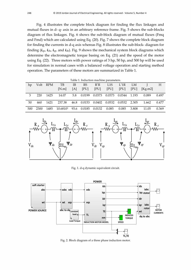
parameters, electromagnetic torque and load torque defined by Eq. (13). Fig. 1 shows
the dynamic equivalent circuit, while Fig. 2 illustrates a block diagram of a 3-phase
induction motor.
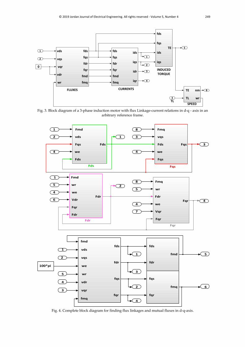
Fig. 3 shows the induction motor d-q model, which represents the induction
motor using d-q axes in an arbitrary reference frame. This model consists of two main
parts: the electrical model and the dynamical model as depicted in Eqs. (11-20).
248 © 2019 Jordan Journal of Electrical Engineering. All rights reserved - Volume 5, Number 4
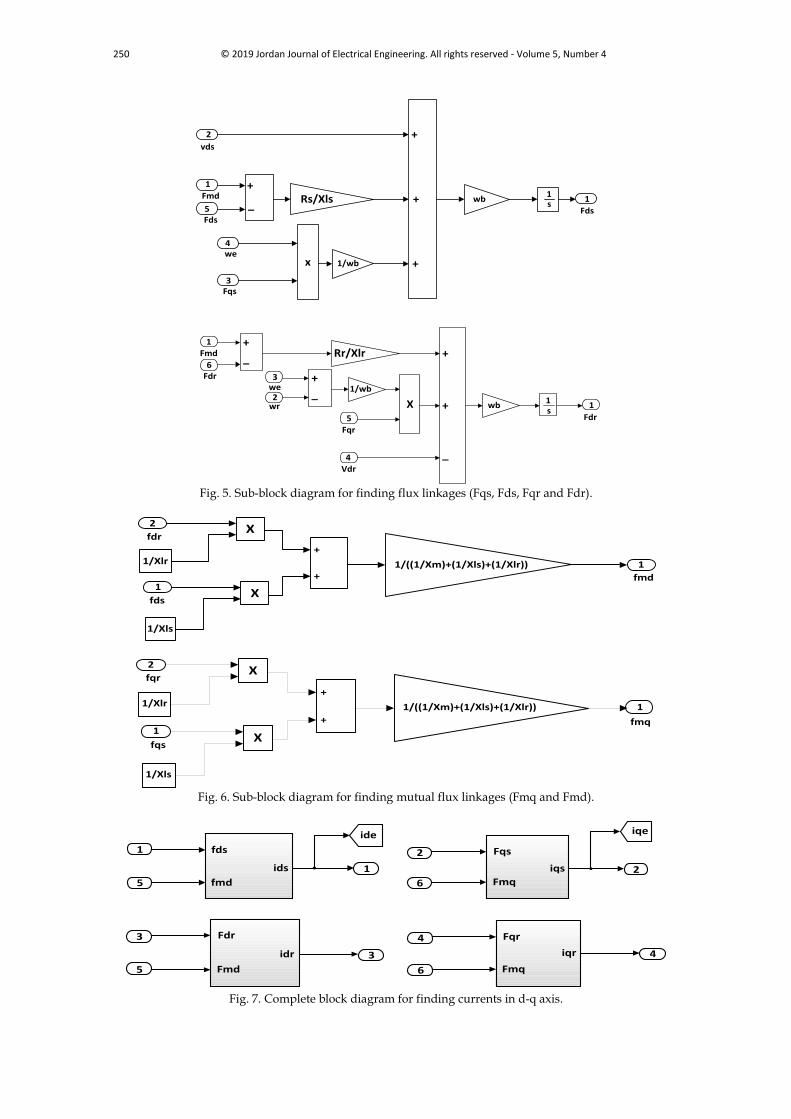
Fig. 4 illustrates the complete block diagram for finding the flux linkages and
mutual fluxes in d- q- axis in an arbitrary reference frame. Fig. 5 shows the sub-blocks
diagram of flux linkages. Fig. 6 shows the sub-block diagram of mutual fluxes (Fmq
and Fmd) which are calculated using Eq. (20). Fig. 7 shows the complete block diagram
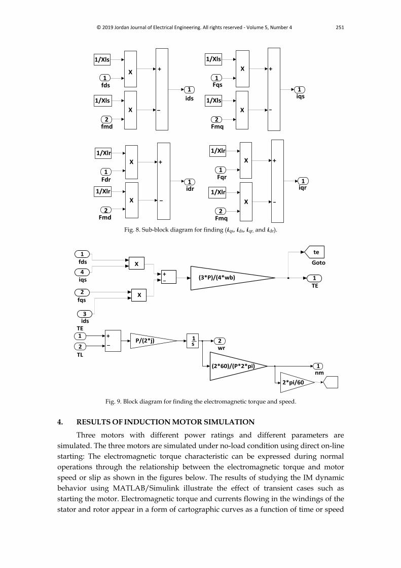
for finding the currents in d-q axis whereas Fig. 8 illustrates the sub-block- diagram for
finding (𝒊qs, 𝒊ds, 𝒊qr, and 𝒊dr). Fig. 9 shows the mechanical system block diagrams which
determine the electromagnetic torque basing on Eq. (21) and the speed of the motor
using Eq. (22). Three motors with power ratings of 3 hp, 50 hp, and 500 hp will be used
for simulation in normal cases with a balanced voltage operation and starting method
operation. The parameters of these motors are summarized in Table 1.
Table 1. Induction machine parameters.
hp Volt RPM TB [N.m]
IB [A]
RS [PU]
R’R [PU]
L1S [PU]
L’1R [PU]
LM [PU]
J [Kg.m2]
H
3 220 1425 14.07 5.8 0.0199 0.0373 0.0373 0.0344 1.193 0.089 0.497
50 460 1421 237.38 46.8 0.0153 0.0402 0.0532 0.0532 2.305 1.662 0.477
500 2300 1485 10.68102 93.6 0.0185 0.0132 0.085 0.085 3.808 11.05 0.369
VdrΨdrΨdsVds
+ +_
Ids Idr
Lm
R a R rL1s L1r
ΨqrΨqsVqs
+ +_
Iqs Iqr
Lm
R a R rL1s L1r
Vqr
_ _
Fig. 1. d-q dynamic equivalent circuit.
INDUCED TORQUE
SPEED
TL,TE
vds
vqs
TL
ids
iqs
idr
iqr
TE
nm
INDUCTION MOTOR MODEL
ids
iqs
idr
iqr
wt
iabc stator
iabc rotor
dq to abc
vabc
wt
vds
vqs
abc to dq ROTOR CURRENTS
abc
wt
soft starter
POWER SOURCE
Tl
constant load
Load Torque
POWER
Fig. 2. Block diagram of a three phase induction motor.
© 2019 Jordan Journal of Electrical Engineering. All rights reserved - Volume 5, Number 4 249
6
5
4
3
2
1
TE
TL
nm
wr
SPEED
fds
fqs
ids
iqs
TE
INDUCED TORQUE
fds
fqs
fdr
fqr
fmd
fmq
ids
iqs
idr
iqr
CURRENTS
vds
vqs
vqr
vdr
wr
fds
fqs
fdr
fqr
fmd
fmq
FLUXES
1
2
0
3TL
Fig. 3. Block diagram of a 3-phase induction motor with flux Linkage-current relations in d-q - axis in an
arbitrary reference frame.
1
1 Fmq
vqs
Fds
we
Fqs
Fqs
Fqs
Fmq
wr
Fdr
we
Vqr
Fqr
Fqr
Fqr
Fmd
vds
Fqs
we
Fds
Fds
Fds
Fmd
wr
we
Vdr
Fqr
Fdr
Fdr
Fdr
8
2 3
4
5
6
7
4
1
8
4
45
3
2
4
fds
fdr
fmd
fqs
fqr
fmq
4
3
1
2
2
1
3
4
5
6
5
100*pi
fmd
vds
vqs
we
wr
vdr
vqr
fmq
fds
fdr
fqs
fqr
Fig. 4. Complete block diagram for finding flux linkages and mutual fluxes in d-q-axis.
250 © 2019 Jordan Journal of Electrical Engineering. All rights reserved - Volume 5, Number 4
1
Fds
1sRs/Xls
1/wb
wb5Fds
4we
3Fqs
2
vds
1
Fmd+
_
x +
+
+
1
Fdr
1s
wb
1/wb
Rr/Xlr
4Vdr
6Fdr 3
we
5
Fqr
2wr
1Fmd
+
_
X
+
+
+_
_
Fig. 5. Sub-block diagram for finding flux linkages (Fqs, Fds, Fqr and Fdr).
1
fmd
1/((1/Xm)+(1/Xls)+(1/Xlr))
1/Xls
1/Xlr
2
fdr
1
fds
+
+
X
X
1
fmq
1/((1/Xm)+(1/Xls)+(1/Xlr))
1/Xls
1/Xlr
2
fqr
1
fqs
X
X
+
+
Fig. 6. Sub-block diagram for finding mutual flux linkages (Fmq and Fmd).
4
Fqr
Fmq
iqr
4
6
3
Fdr
Fmd
idr
3
5
2
Fqs
Fmq
iqs
2
6
iqe
1
1
fds
fmd
ids
5
ide
Fig. 7. Complete block diagram for finding currents in d-q axis.
© 2019 Jordan Journal of Electrical Engineering. All rights reserved - Volume 5, Number 4 251
1iqr
1/Xlr
1/Xlr
2Fmq
1Fqr
+X
X
1iqs
1/Xls
1/Xls
2Fmq
1Fqs
X
X
+
1idr1/Xlr
1/Xlr
2Fmd
1Fdr
X
X
+
1
ids1/Xls
1/Xls
2fmd
1fds
X
X +
Fig. 8. Sub-block diagram for finding (𝒊qs, 𝒊ds, 𝒊qr, and 𝒊dr).
2wr
1s
P/(2*j)
(2*60)/(P*2*pi)
2
TL
1TE
+
1TE
(3*P)/(4*wb)
3ids
2
fqs
4iqs
1fds
te
GotoX
X
+
1nm
2*pi/60
Fig. 9. Block diagram for finding the electromagnetic torque and speed.
4. RESULTS OF INDUCTION MOTOR SIMULATION
Three motors with different power ratings and different parameters are
simulated. The three motors are simulated under no-load condition using direct on-line
starting: The electromagnetic torque characteristic can be expressed during normal
operations through the relationship between the electromagnetic torque and motor
speed or slip as shown in the figures below. The results of studying the IM dynamic
behavior using MATLAB/Simulink illustrate the effect of transient cases such as
starting the motor. Electromagnetic torque and currents flowing in the windings of the
stator and rotor appear in a form of cartographic curves as a function of time or speed
252 © 2019 Jordan Journal of Electrical Engineering. All rights reserved - Volume 5, Number 4
with a large strike (in-rush) current that arises with a few cycles. More oscillations and
high peak values appear as a result of the high instantaneous input current drawn by a
motor during the initial starting process, where the induction motor behaves as a
transformer with a short-circuited rotor until it begins to rotate. Currents flowing in the
motor's windings during transient cases such as the starting process contain two
components; a DC component and AC component. These are formed as a result of
I’-sub transient, I'-transient and Ι-steady state currents which correspond to the
reactance values. The DC component will fade to zero at the end of an electromagnetic
transient case depending on the winding time constant. Analyzing the effect of the
motor parameters in transient cases gives a perception of the quality and characteristic
of transient cases and situations for defining the peak value of the torque, strike current
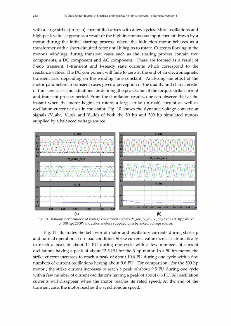
and transient process period. From the simulation results, one can observe that at the
instant when the motor begins to rotate, a large strike (in-rush) current as well as
oscillation current arises in the stator. Fig. 10 shows the dynamic voltage conversion
signals (V_abc, V_αβ, and V_dq) of both the 50 hp and 500 hp simulated motors
supplied by a balanced voltage source.
(a) (b)
V_abc V_abc
V_alpha_beta V_alpha_beta
V_dq V_dq
1.52 1.54 1.56 1.58 1.60 1.62 1.64 1.66 1.68
-1.5
-1
0
0.5
1
1.5
-0.5
-1
-0.5
0
0.5
1
1.5
-1.5
-0.5
0
0.5
1
1.5
1.52 1.54 1.56 1.58 1.60 1.62-0.5
0
0.5
1
1.5
-2
2
-1
0
1
-1.5
-1
-0.5
0
0.5
11.5
1.70
Fig. 10. Dynamic performance of voltage conversion signals (V_abc, V_αβ, V_dq) for: a) 50 hp/ 460V;
b) 500 hp/2300V induction motors supplied by a balanced voltage source.
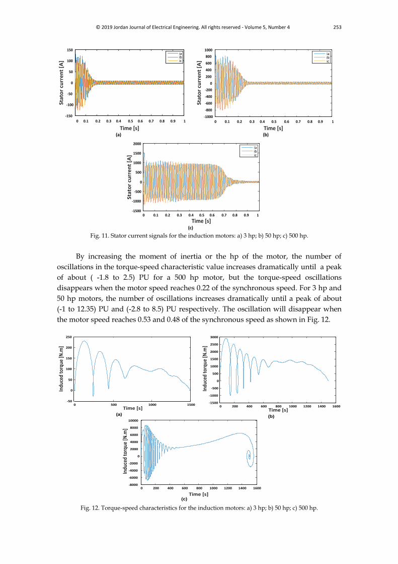
Fig. 11 illustrates the behavior of motor and oscillatory currents during start-up
and normal operation at no-load condition. Strike currents value increases dramatically
to reach a peak of about 14 PU during one cycle with a few numbers of current
oscillations having a peak of about 13.5 PU for the 3 hp motor. In a 50 hp motor, the
strike current increases to reach a peak of about 10.6 PU during one cycle with a few
numbers of current oscillations having about 9.6 PU. For comparison , for the 500 hp
motor , the strike current increases to reach a peak of about 9.5 PU during one cycle
with a few number of current oscillations having a peak of about 6.6 PU. All oscillation
currents will disappear when the motor reaches its rated speed. At the end of the
transient case, the motor reaches the synchronous speed.
© 2019 Jordan Journal of Electrical Engineering. All rights reserved - Volume 5, Number 4 253
0 0.1 0.2 0.3 0.4 0.5 0.6 0.7 0.8 0.9 1
-150
-100
-50
0
50
100
150
Time [s]
Sta
tor
curr
en
t [A
]
iaibic
0 0.1 0.2 0.3 0.4 0.5 0.6 0.7 0.8 0.9 1-1000
-800
-600
-400
-200
0
200
400
600
800
1000
Time [s]
Sta
tor
curr
en
t [A
]
iaibic
0 0.1 0.2 0.3 0.4 0.5 0.6 0.7 0.8 0.9 1-1500
-1000
-500
0
500
1000
1500
2000
Time [s]
Sta
tor
curr
en
t [A
]
iaibic
(a) (b)
(c) Fig. 11. Stator current signals for the induction motors: a) 3 hp; b) 50 hp; c) 500 hp.
By increasing the moment of inertia or the hp of the motor, the number of
oscillations in the torque-speed characteristic value increases dramatically until a peak
of about ( -1.8 to 2.5) PU for a 500 hp motor, but the torque-speed oscillations
disappears when the motor speed reaches 0.22 of the synchronous speed. For 3 hp and
50 hp motors, the number of oscillations increases dramatically until a peak of about
(-1 to 12.35) PU and (-2.8 to 8.5) PU respectively. The oscillation will disappear when
the motor speed reaches 0.53 and 0.48 of the synchronous speed as shown in Fig. 12.
0 500 1000 1500-50
0
50
100
150
200
250
Time [s]
Indu
ced
torq
ue [N
.m]
0 200 400 600 800 1000 1200 1400 1600-1500
-1000
-500
0
500
1000
1500
2000
2500
3000
Time [s]
Indu
ced
torq
ue [N
.m]
0 200 400 600 800 1000 1200 1400 1600-8000
-6000
-4000
-2000
0
2000
4000
6000
8000
10000
Time [s]
Indu
ced
torq
ue [N
.m]
(a)(b)
(c) Fig. 12. Torque-speed characteristics for the induction motors: a) 3 hp; b) 50 hp; c) 500 hp.
254 © 2019 Jordan Journal of Electrical Engineering. All rights reserved - Volume 5, Number 4
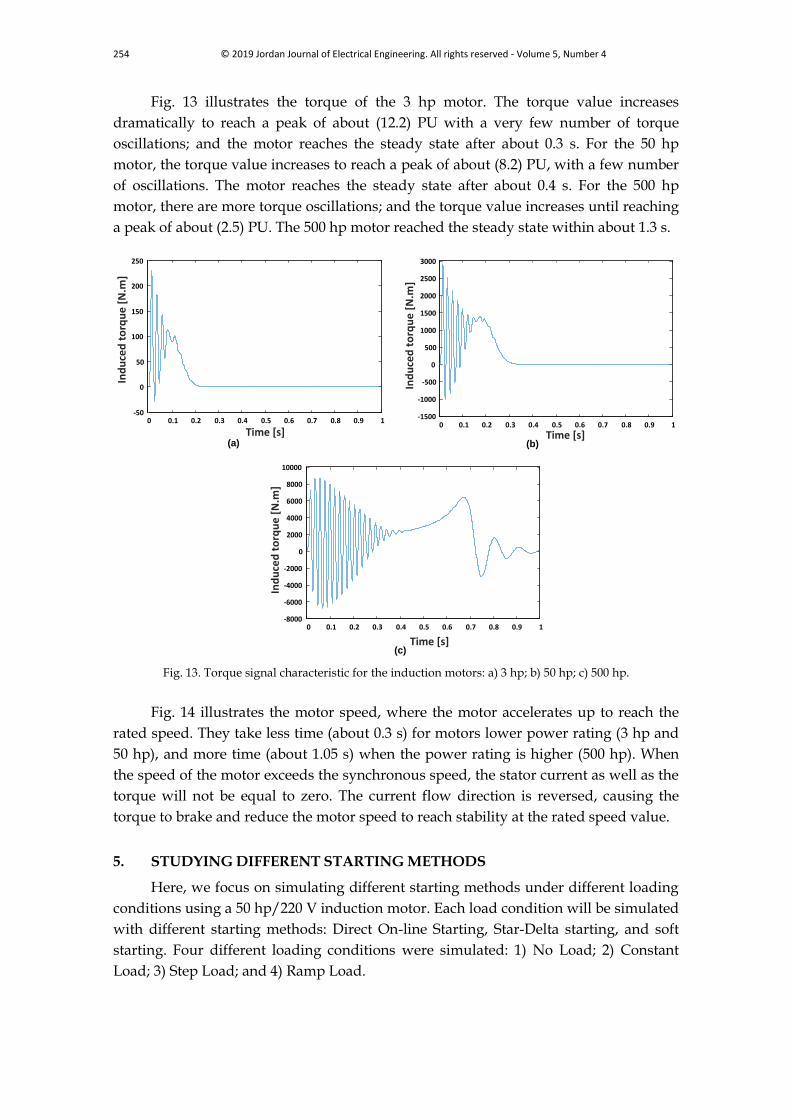
Fig. 13 illustrates the torque of the 3 hp motor. The torque value increases
dramatically to reach a peak of about (12.2) PU with a very few number of torque
oscillations; and the motor reaches the steady state after about 0.3 s. For the 50 hp
motor, the torque value increases to reach a peak of about (8.2) PU, with a few number
of oscillations. The motor reaches the steady state after about 0.4 s. For the 500 hp
motor, there are more torque oscillations; and the torque value increases until reaching
a peak of about (2.5) PU. The 500 hp motor reached the steady state within about 1.3 s.
0 0.1 0.2 0.3 0.4 0.5 0.6 0.7 0.8 0.9 1-50
0
50
100
150
200
250
Time [s]
Ind
uce
d t
orq
ue
[N
.m]
0 0.1 0.2 0.3 0.4 0.5 0.6 0.7 0.8 0.9 1-1500
-1000
-500
0
500
1000
1500
2000
2500
3000
Time [s]
Ind
uce
d t
orq
ue
[N
.m]
0 0.1 0.2 0.3 0.4 0.5 0.6 0.7 0.8 0.9 1-8000
-6000
-4000
-2000
0
2000
4000
6000
8000
10000
Time [s]
Ind
uce
d t
orq
ue
[N
.m]
(a) (b)
(c)
Fig. 13. Torque signal characteristic for the induction motors: a) 3 hp; b) 50 hp; c) 500 hp.
Fig. 14 illustrates the motor speed, where the motor accelerates up to reach the
rated speed. They take less time (about 0.3 s) for motors lower power rating (3 hp and
50 hp), and more time (about 1.05 s) when the power rating is higher (500 hp). When
the speed of the motor exceeds the synchronous speed, the stator current as well as the
torque will not be equal to zero. The current flow direction is reversed, causing the
torque to brake and reduce the motor speed to reach stability at the rated speed value.
5. STUDYING DIFFERENT STARTING METHODS
Here, we focus on simulating different starting methods under different loading
conditions using a 50 hp/220 V induction motor. Each load condition will be simulated
with different starting methods: Direct On-line Starting, Star-Delta starting, and soft
starting. Four different loading conditions were simulated: 1) No Load; 2) Constant
Load; 3) Step Load; and 4) Ramp Load.
© 2019 Jordan Journal of Electrical Engineering. All rights reserved - Volume 5, Number 4 255
0 0.1 0.2 0.3 0.4 0.5 0.6 0.7 0.8 0.9 10
500
1000
1500
Time [s]
Spee
d [R
PM]
0 0.1 0.2 0.3 0.4 0.5 0.6 0.7 0.8 0.9 10
200
400
600
800
1000
1200
1400
1600
Time [s]
Spee
d [R
PM]
0 0.1 0.2 0.3 0.4 0.5 0.6 0.7 0.8 0.9 10
200
400
600
800
1000
1200
1400
1600
Time [s]
Spee
d [R
PM]
(a) (b)
(c)
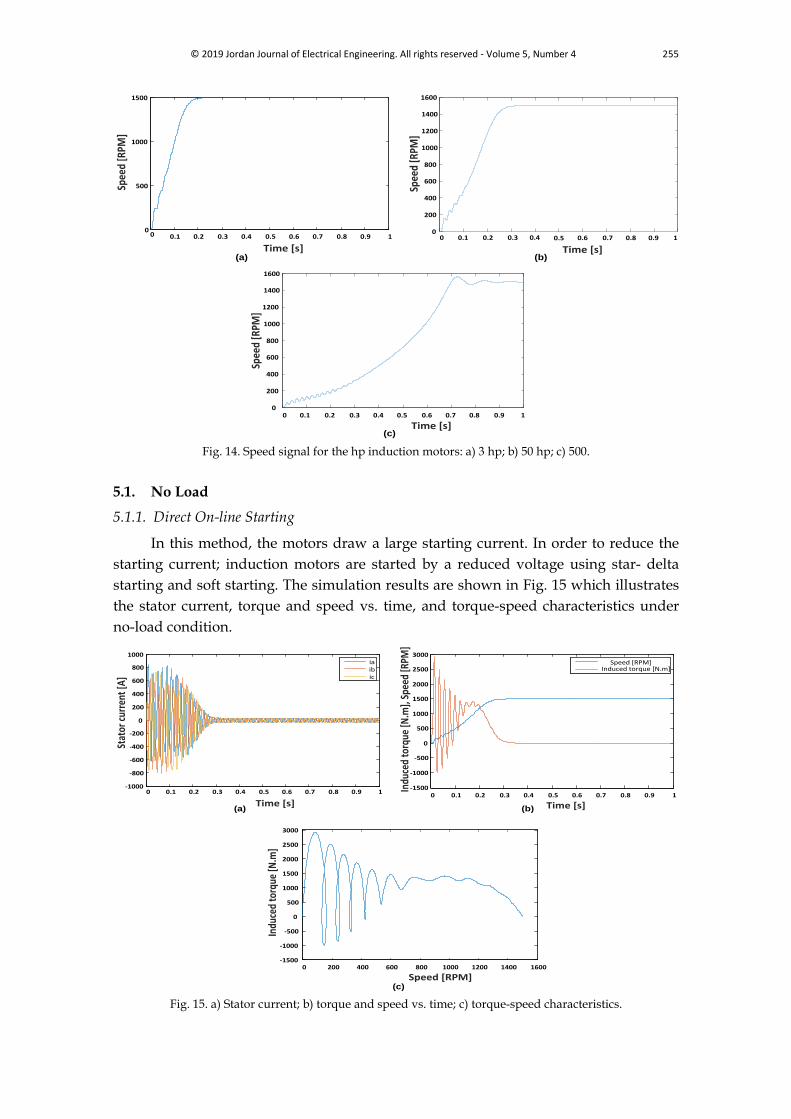
Fig. 14. Speed signal for the hp induction motors: a) 3 hp; b) 50 hp; c) 500.
5.1. No Load
5.1.1. Direct On-line Starting
In this method, the motors draw a large starting current. In order to reduce the
starting current; induction motors are started by a reduced voltage using star- delta
starting and soft starting. The simulation results are shown in Fig. 15 which illustrates
the stator current, torque and speed vs. time, and torque-speed characteristics under
no-load condition.
0 0.1 0.2 0.3 0.4 0.5 0.6 0.7 0.8 0.9 1-1000
-800
-600
-400
-200
0
200
400
600
800
1000
Time [s]
Stat
or c
urre
nt [A
]
iaibic
0 200 400 600 800 1000 1200 1400 1600-1500
-1000
-500
0
500
1000
1500
2000
2500
3000
Speed [RPM]
Indu
ced
torq
ue [N
.m]
(a)
(c)
0 0.1 0.2 0.3 0.4 0.5 0.6 0.7 0.8 0.9 1-1500
-1000
-500
0
500
1000
1500
2000
2500
3000
Time [s]
Indu
ced
torq
ue [N
.m],
Spee
d [R
PM]
Induced torque [N.m]Speed [RPM]
(b)
Fig. 15. a) Stator current; b) torque and speed vs. time; c) torque-speed characteristics.
256 © 2019 Jordan Journal of Electrical Engineering. All rights reserved - Volume 5, Number 4
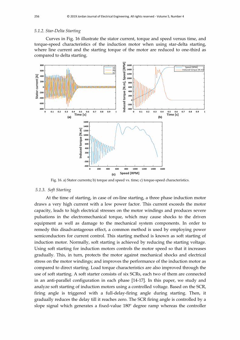
5.1.2. Star-Delta Starting
Curves in Fig. 16 illustrate the stator current, torque and speed versus time, and torque-speed characteristics of the induction motor when using star-delta starting, where line current and the starting torque of the motor are reduced to one-third as compared to delta starting.
0 0.1 0.2 0.3 0.4 0.5 0.6 0.7 0.8 0.9 1-800
-600
-400
-200
0
200
400
600
800
Time [s]
Stat
or
curr
ent
[A]
iaibic
0 0.1 0.2 0.3 0.4 0.5 0.6 0.7 0.8 0.9 1-400
-200
0
200
400
600
800
1000
1200
1400
1600
Time [s]
Ind
uce
d t
orq
ue
[N.m
], S
pee
d [
RP
M]
Induced torque [N.m]Speed [RPM]
0 200 400 600 800 1000 1200 1400 1600
-400
-200
0
200
400
600
800
1000
1200
1400
1600
Speed [RPM]
Ind
uce
d t
orq
ue
[N.m
]
(a) (b)
(c)
Fig. 16. a) Stator currents; b) torque and speed vs. time; c) torque-speed characteristics.
5.1.3. Soft Starting
At the time of starting, in case of on-line starting, a three phase induction motor
draws a very high current with a low power factor. This current exceeds the motor
capacity, leads to high electrical stresses on the motor windings and produces severe
pulsations in the electromechanical torque, which may cause shocks to the driven
equipment as well as damage to the mechanical system components. In order to
remedy this disadvantageous effect, a common method is used by employing power
semiconductors for current control. This starting method is known as soft starting of
induction motor. Normally, soft starting is achieved by reducing the starting voltage.
Using soft starting for induction motors controls the motor speed so that it increases
gradually. This, in turn, protects the motor against mechanical shocks and electrical
stress on the motor windings; and improves the performance of the induction motor as
compared to direct starting. Load torque characteristics are also improved through the
use of soft starting. A soft starter consists of six SCRs, each two of them are connected
in an anti-parallel configuration in each phase [14-17]. In this paper, we study and
analyze soft starting of induction motors using a controlled voltage. Based on the SCR,
firing angle is triggered with a full-delay-firing angle during starting. Then, it
gradually reduces the delay till it reaches zero. The SCR firing angle is controlled by a
slope signal which generates a fixed-value 180º degree ramp whereas the controller
© 2019 Jordan Journal of Electrical Engineering. All rights reserved - Volume 5, Number 4 257
generates another signal which is then compared with the ramp signal. This leads to
reduce the voltage during starting which is then gradually built-up until reaching a full
supply voltage. The reference signal value gradually increases, leading to eliminating
the starting torque pulsations, so that the motor starts slowly and reaches its full rated
speed gradually.
5.1.4. Simulation Results
Figs. 17-19 illustrate the simulation results on terms of three phase induction
motor waveforms of voltage, current, torque, and speed when using soft starting at
no-load with generating -180°, -360º, and -540º ramps respectively.
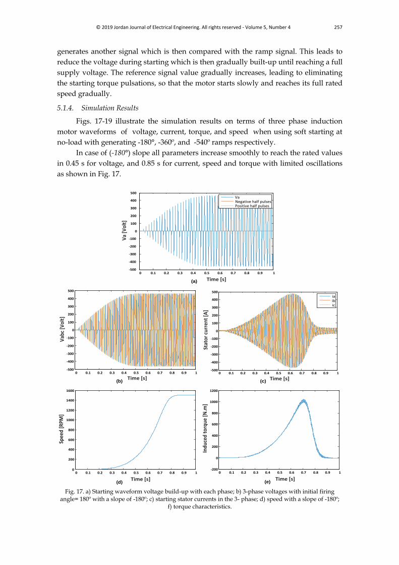
In case of (-180°) slope all parameters increase smoothly to reach the rated values
in 0.45 s for voltage, and 0.85 s for current, speed and torque with limited oscillations
as shown in Fig. 17.
0 0.1 0.2 0.3 0.4 0.5 0.6 0.7 0.8 0.9 1-500
-400
-300
-200
-100
0
100
200
300
400
500
Time [s]
Va
[Vol
t]
VaNegative half pulsesPositive half pulses
0 0.1 0.2 0.3 0.4 0.5 0.6 0.7 0.8 0.9 1-500
-400
-300
-200
-100
0
100
200
300
400
500
Time [s]
Vab
c [V
olt]
0 0.1 0.2 0.3 0.4 0.5 0.6 0.7 0.8 0.9 1-500
-400
-300
-200
-100
0
100
200
300
400
500
Time [s]
Stat
or c
urre
nt [
A]
iaibic
0 0.1 0.2 0.3 0.4 0.5 0.6 0.7 0.8 0.9 10
200
400
600
800
1000
1200
1400
1600
Time [s]
Spee
d [R
PM]
0 0.1 0.2 0.3 0.4 0.5 0.6 0.7 0.8 0.9 1-200
0
200
400
600
800
1000
1200
Time [s]
Indu
ced
torq
ue [
N.m
]
(a)
(b) (c)
(d) (e)
Fig. 17. a) Starting waveform voltage build-up with each phase; b) 3-phase voltages with initial firing angle= 180º with a slope of -180º; c) starting stator currents in the 3- phase; d) speed with a slope of -180º;
f) torque characteristics.
258 © 2019 Jordan Journal of Electrical Engineering. All rights reserved - Volume 5, Number 4
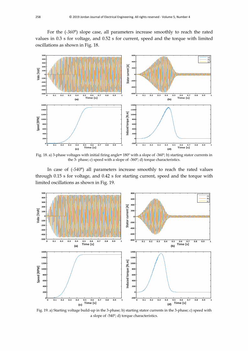
For the (-360°) slope case, all parameters increase smoothly to reach the rated
values in 0.3 s for voltage, and 0.52 s for current, speed and the torque with limited
oscillations as shown in Fig. 18.
0 0.1 0.2 0.3 0.4 0.5 0.6 0.7 0.8 0.9 1-500
-400
-300
-200
-100
0
100
200
300
400
500
Time [s]
Vabc
[Vol
t]
0 0.1 0.2 0.3 0.4 0.5 0.6 0.7 0.8 0.9 1-600
-400
-200
0
200
400
600
Time [s]
Stat
or cu
rren
t [A]
iaibic
0 0.1 0.2 0.3 0.4 0.5 0.6 0.7 0.8 0.9 10
200
400
600
800
1000
1200
1400
1600
Time [s]
Spee
d [R
PM]
0 0.1 0.2 0.3 0.4 0.5 0.6 0.7 0.8 0.9 1-200
0
200
400
600
800
1000
1200
1400
Time [s]
Indu
ced
torq
ue [N
.m]
(d)(c)
(b)(a)
Fig. 18. a) 3-phase voltages with initial firing angle= 180º with a slope of -360º; b) starting stator currents in
the 3- phase; c) speed with a slope of -360º; d) torque characteristics.
In case of (-540°) all parameters increase smoothly to reach the rated values
through 0.15 s for voltage, and 0.42 s for starting current, speed and the torque with
limited oscillations as shown in Fig. 19.
0 0.1 0.2 0.3 0.4 0.5 0.6 0.7 0.8 0.9 1-500
-400
-300
-200
-100
0
100
200
300
400
500
Time [s]
Vab
c [V
olt]
0 0.1 0.2 0.3 0.4 0.5 0.6 0.7 0.8 0.9 1-800
-600
-400
-200
0
200
400
600
800
Time [s]
Stat
or c
urre
nt [A
]
iaibic
(b)(a)
0 0.1 0.2 0.3 0.4 0.5 0.6 0.7 0.8 0.9 10
200
400
600
800
1000
1200
1400
1600
Time [s]
Spee
d [R
PM]
0 0.1 0.2 0.3 0.4 0.5 0.6 0.7 0.8 0.9 1-200
0
200
400
600
800
1000
1200
1400
Time [s]
Indu
ced
torq
ue [N
.m]
(d)(c) Fig. 19. a) Starting voltage build-up in the 3-phase; b) starting stator currents in the 3-phase; c) speed with
a slope of -540º; d) torque characteristics.
© 2019 Jordan Journal of Electrical Engineering. All rights reserved - Volume 5, Number 4 259
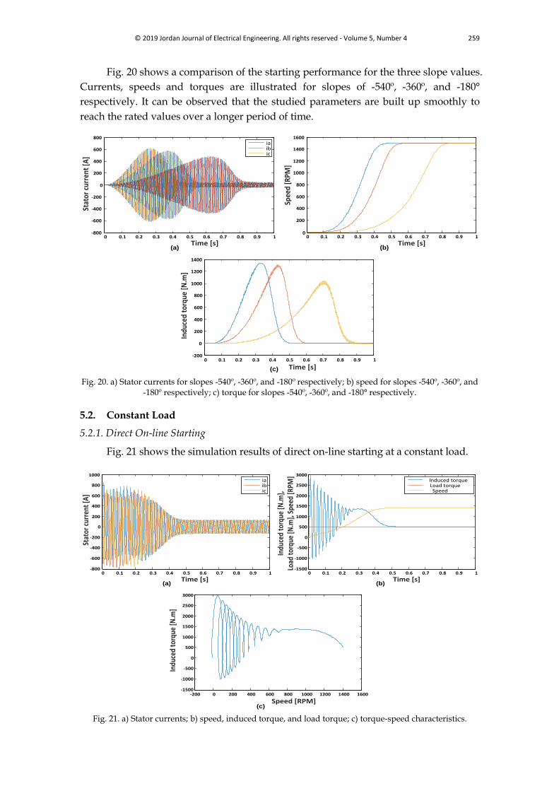
Fig. 20 shows a comparison of the starting performance for the three slope values.
Currents, speeds and torques are illustrated for slopes of -540º, -360º, and -180°
respectively. It can be observed that the studied parameters are built up smoothly to
reach the rated values over a longer period of time.
0 0.1 0.2 0.3 0.4 0.5 0.6 0.7 0.8 0.9 1-800
-600
-400
-200
0
200
400
600
800
Time [s]
Stat
or c
urre
nt [A
]
iaibic
0 0.1 0.2 0.3 0.4 0.5 0.6 0.7 0.8 0.9 10
200
400
600
800
1000
1200
1400
1600
Time [s]
Spee
d [R
PM]
0 0.1 0.2 0.3 0.4 0.5 0.6 0.7 0.8 0.9 1-200
0
200
400
600
800
1000
1200
1400
Time [s]
Indu
ced
torq
ue [N
.m]
(a) (b)
(c)
Fig. 20. a) Stator currents for slopes -540º, -360º, and -180º respectively; b) speed for slopes -540º, -360º, and -180º respectively; c) torque for slopes -540º, -360º, and -180° respectively.
5.2. Constant Load
5.2.1. Direct On-line Starting
Fig. 21 shows the simulation results of direct on-line starting at a constant load.
0 0.1 0.2 0.3 0.4 0.5 0.6 0.7 0.8 0.9 1-800
-600
-400
-200
0
200
400
600
800
1000
Time [s]
Stat
or c
urre
nt [A
]
iaibic
0 0.1 0.2 0.3 0.4 0.5 0.6 0.7 0.8 0.9 1-1500
-1000
-500
0
500
1000
1500
2000
2500
3000
Time [s]
Indu
ced
torq
ue [N
.m],
Load
torq
ue [N
.m],
Spee
d [R
PM]
Induced torque Load torqueSpeed
-200 0 200 400 600 800 1000 1200 1400 1600-1500
-1000
-500
0
500
1000
1500
2000
2500
3000
Speed [RPM]
Indu
ced
torq
ue [N
.m]
(a) (b)
(c)
Fig. 21. a) Stator currents; b) speed, induced torque, and load torque; c) torque-speed characteristics.
260 © 2019 Jordan Journal of Electrical Engineering. All rights reserved - Volume 5, Number 4
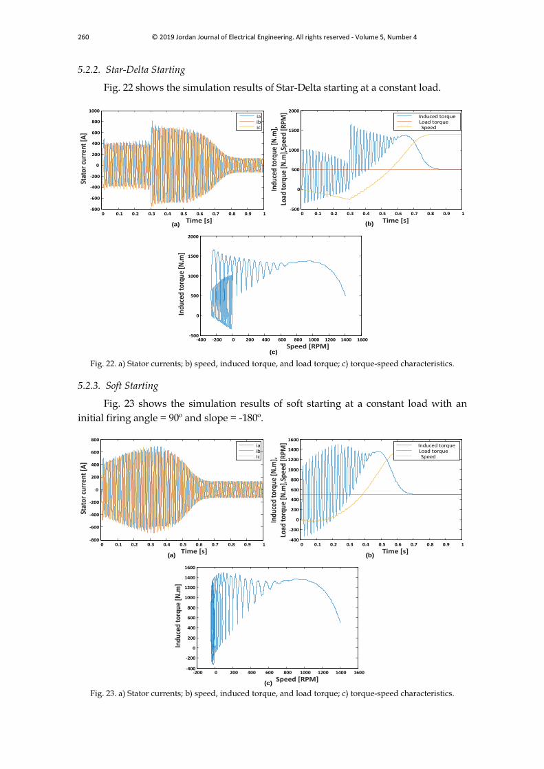
5.2.2. Star-Delta Starting
Fig. 22 shows the simulation results of Star-Delta starting at a constant load.
0 0.1 0.2 0.3 0.4 0.5 0.6 0.7 0.8 0.9 1-800
-600
-400
-200
0
200
400
600
800
1000
Time [s]
Stat
or c
urre
nt [A
]
iaibic
0 0.1 0.2 0.3 0.4 0.5 0.6 0.7 0.8 0.9 1-500
0
500
1000
1500
2000
Time [s]
Indu
ced
torq
ue [N
.m],
Load
tor
que
[N.m
],Sp
eed
[RPM
]
Induced torqueLoad torqueSpeed
-400 -200 0 200 400 600 800 1000 1200 1400 1600-500
0
500
1000
1500
2000
Speed [RPM]
Indu
ced
torq
ue [N
.m]
(a) (b)
(c) Fig. 22. a) Stator currents; b) speed, induced torque, and load torque; c) torque-speed characteristics.
5.2.3. Soft Starting
Fig. 23 shows the simulation results of soft starting at a constant load with an
initial firing angle = 90º and slope = -180º.
0 0.1 0.2 0.3 0.4 0.5 0.6 0.7 0.8 0.9 1-800
-600
-400
-200
0
200
400
600
800
Time [s]
Stat
or c
urre
nt [A
]
iaibic
0 0.1 0.2 0.3 0.4 0.5 0.6 0.7 0.8 0.9 1-400
-200
0
200
400
600
800
1000
1200
1400
1600
Time [s]
Indu
ced
torq
ue [N
.m],
Load
tor
que
[N.m
],Sp
eed
[RPM
]
Induced torque Load torqueSpeed
-200 0 200 400 600 800 1000 1200 1400 1600-400
-200
0
200
400
600
800
1000
1200
1400
1600
Speed [RPM]
Indu
ced
torq
ue [N
.m]
(a) (b)
(c) Fig. 23. a) Stator currents; b) speed, induced torque, and load torque; c) torque-speed characteristics.
© 2019 Jordan Journal of Electrical Engineering. All rights reserved - Volume 5, Number 4 261
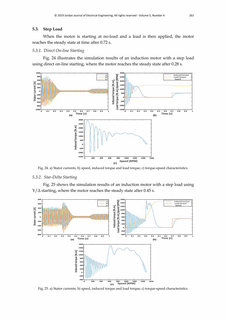
5.3. Step Load
When the motor is starting at no-load and a load is then applied, the motor
reaches the steady state at time after 0.72 s.
5.3.1. Direct On-line Starting
Fig. 24 illustrates the simulation results of an induction motor with a step load
using direct on-line starting, where the motor reaches the steady state after 0.28 s.
0 0.1 0.2 0.3 0.4 0.5 0.6 0.7 0.8 0.9 1-1000
-800
-600
-400
-200
0
200
400
600
800
1000
Time [s]
Stat
or c
urre
nt [A
]
iaibic
0 0.1 0.2 0.3 0.4 0.5 0.6 0.7 0.8 0.9 1-1500
-1000
-500
0
500
1000
1500
2000
2500
3000
Time [s]In
duce
d to
rque
[N.m
],Lo
ad to
rque
[N.m
],Spe
ed [R
PM]
Induced torqueLoad torqueSpeed
0 200 400 600 800 1000 1200 1400 1600-1500
-1000
-500
0
500
1000
1500
2000
2500
3000
Speed [RPM]
Indu
ced
torq
ue [N
.m]
(a) (b)
(c) Fig. 24. a) Stator currents; b) speed, induced torque and load torque; c) torque-speed characteristics.
5.3.2. Star-Delta Starting
Fig. 25 shows the simulation results of an induction motor with a step load using
Y/Δ starting, where the motor reaches the steady state after 0.45 s.
0 0.1 0.2 0.3 0.4 0.5 0.6 0.7 0.8 0.9 1-800
-600
-400
-200
0
200
400
600
800
Time [s]
Stat
or cu
rren
t [A]
iaibic
0 0.1 0.2 0.3 0.4 0.5 0.6 0.7 0.8 0.9 1-400
-200
0
200
400
600
800
1000
1200
1400
1600
Time [s]
Indu
ced
torq
ue [N
.m],
Load
torq
ue [N
.m],S
peed
[RPM
]
Induced torqueLoad torqueSpeed
0 200 400 600 800 1000 1200 1400 1600-400
-200
0
200
400
600
800
1000
1200
1400
1600
Speed [RPM]
Indu
ced
torq
ue [N
.m]
(c)
(a) (b)
Fig. 25. a) Stator currents; b) speed, induced torque and load torque; c) torque-speed characteristics.
262 © 2019 Jordan Journal of Electrical Engineering. All rights reserved - Volume 5, Number 4
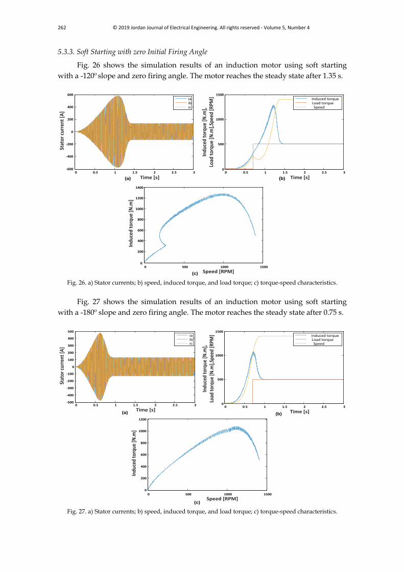
5.3.3. Soft Starting with zero Initial Firing Angle
Fig. 26 shows the simulation results of an induction motor using soft starting
with a -120º slope and zero firing angle. The motor reaches the steady state after 1.35 s.
0 0.5 1 1.5 2 2.5 3-600
-400
-200
0
200
400
600
Time [s]
Stat
or c
urre
nt [
A]
iaibic
0 0.5 1 1.5 2 2.5 30
500
1000
1500
Time [s]
Indu
ced
torq
ue [
N.m
],Lo
ad t
orqu
e [N
.m],
Spee
d [R
PM]
Induced torque Load torque Speed
0 500 1000 15000
200
400
600
800
1000
1200
1400
Speed [RPM]
Indu
ced
torq
ue [
N.m
]
(a) (b)
(c)
Fig. 26. a) Stator currents; b) speed, induced torque, and load torque; c) torque-speed characteristics.
Fig. 27 shows the simulation results of an induction motor using soft starting
with a -180º slope and zero firing angle. The motor reaches the steady state after 0.75 s.
0 0.5 1 1.5 2 2.5 3-500
-400
-300
-200
-100
0
100
200
300
400
500
Time [s]
Stat
or c
urre
nt [A
]
iaibic
0 0.5 1 1.5 2 2.5 30
500
1000
1500
Time [s]
Indu
ced
torq
ue [N
.m],
Load
torq
ue [N
.m],
Spee
d [R
PM]
Induced torqueLoad torqueSpeed
0 500 1000 15000
200
400
600
800
1000
1200
Speed [RPM]
Indu
ced
torq
ue [N
.m]
(c)
(a) (b)
Fig. 27. a) Stator currents; b) speed, induced torque, and load torque; c) torque-speed characteristics.
© 2019 Jordan Journal of Electrical Engineering. All rights reserved - Volume 5, Number 4 263
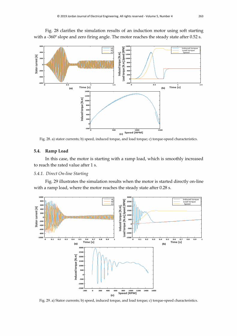
Fig. 28 clarifies the simulation results of an induction motor using soft starting
with a -360º slope and zero firing angle. The motor reaches the steady state after 0.52 s.
0 0.5 1 1.5-600
-400
-200
0
200
400
600
Time [s]
Stat
or cu
rren
t [A]
iaibic
0 0.5 1 1.5-200
0
200
400
600
800
1000
1200
1400
1600
Time [s]
Indu
ced
torq
ue [N
.m],
Load
torq
ue [N
.m],S
peed
[RPM
]
Induced torqueLoad torqueSpeed
0 500 1000 1500-200
0
200
400
600
800
1000
1200
1400
Speed [RPM]
Indu
ced
torq
ue [N
.m]
(a) (b)
(c) Fig. 28. a) stator currents; b) speed, induced torque, and load torque; c) torque-speed characteristics.
5.4. Ramp Load
In this case, the motor is starting with a ramp load, which is smoothly increased
to reach the rated value after 1 s.
5.4.1. Direct On-line Starting
Fig. 29 illustrates the simulation results when the motor is started directly on-line
with a ramp load, where the motor reaches the steady state after 0.28 s.
0 0.1 0.2 0.3 0.4 0.5 0.6 0.7 0.8 0.9 1-1000
-800
-600
-400
-200
0
200
400
600
800
1000
Time [s]
Stat
or c
urre
nt [A
]
iaibic
0 0.1 0.2 0.3 0.4 0.5 0.6 0.7 0.8 0.9 1-1500
-1000
-500
0
500
1000
1500
2000
2500
3000
Time [s]
Indu
ced
torq
ue [N
.m],
Load
torq
ue [N
.m],S
peed
[RPM
]
Induced torque Load torque Speed
-200 0 200 400 600 800 1000 1200 1400 1600
-1500
-1000
-500
0
500
1000
1500
2000
2500
3000
Speed [RPM]
Indu
ced
torq
ue [N
.m]
(a) (b)
(c)
Fig. 29. a) Stator currents; b) speed, induced torque, and load torque; c) torque-speed characteristics.
264 © 2019 Jordan Journal of Electrical Engineering. All rights reserved - Volume 5, Number 4
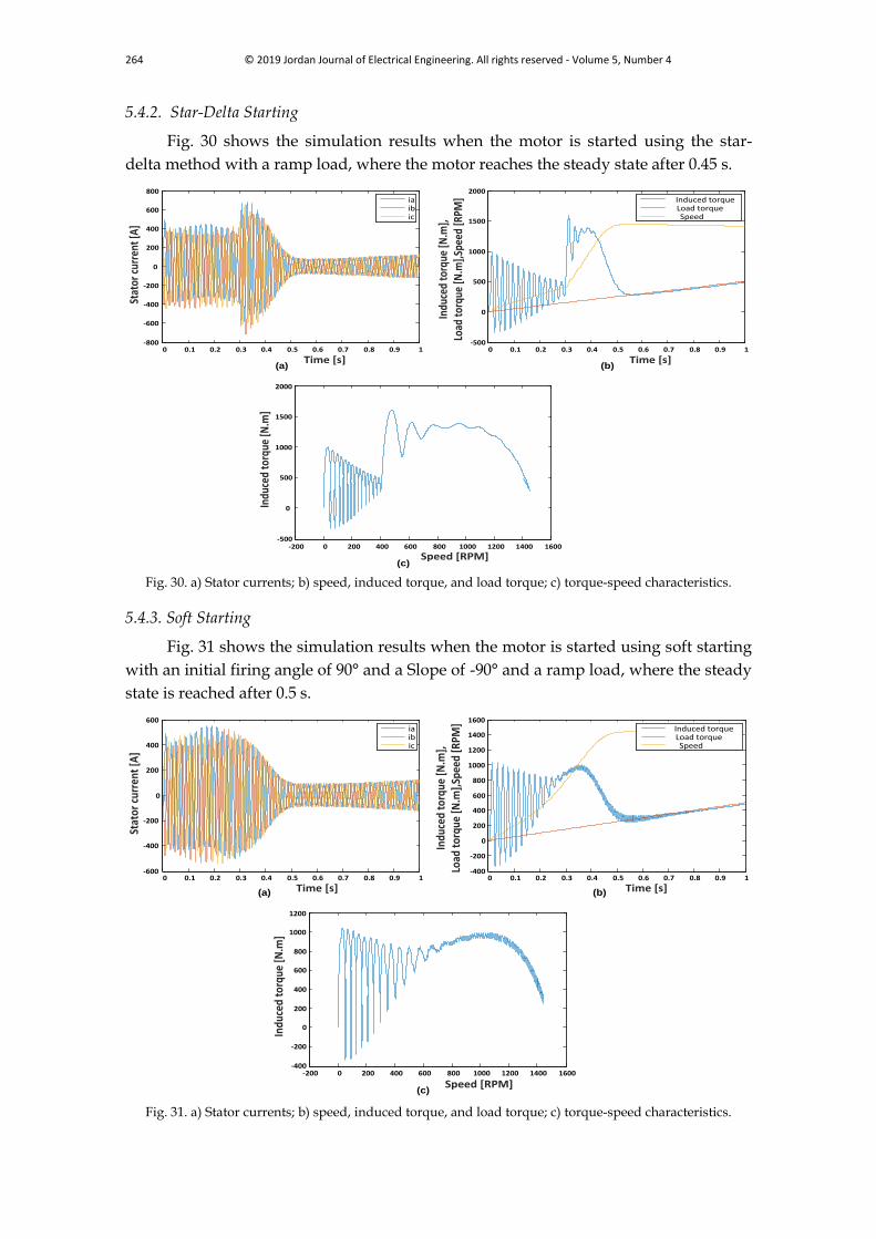
5.4.2. Star-Delta Starting
Fig. 30 shows the simulation results when the motor is started using the star-
delta method with a ramp load, where the motor reaches the steady state after 0.45 s.
0 0.1 0.2 0.3 0.4 0.5 0.6 0.7 0.8 0.9 1-800
-600
-400
-200
0
200
400
600
800
Time [s]
Stat
or c
urre
nt [A
]
iaibic
0 0.1 0.2 0.3 0.4 0.5 0.6 0.7 0.8 0.9 1-500
0
500
1000
1500
2000
Time [s]
Indu
ced
torq
ue [N
.m],
Load
torq
ue [N
.m],S
peed
[RPM
]
Induced torque Load torque Speed
-200 0 200 400 600 800 1000 1200 1400 1600-500
0
500
1000
1500
2000
Speed [RPM]
Indu
ced
torq
ue [N
.m]
(a) (b)
(c) Fig. 30. a) Stator currents; b) speed, induced torque, and load torque; c) torque-speed characteristics.
5.4.3. Soft Starting
Fig. 31 shows the simulation results when the motor is started using soft starting
with an initial firing angle of 90° and a Slope of -90° and a ramp load, where the steady
state is reached after 0.5 s.
0 0.1 0.2 0.3 0.4 0.5 0.6 0.7 0.8 0.9 1-600
-400
-200
0
200
400
600
Time [s]
Stat
or c
urre
nt [A
]
iaibic
0 0.1 0.2 0.3 0.4 0.5 0.6 0.7 0.8 0.9 1-400
-200
0
200
400
600
800
1000
1200
1400
1600
Time [s]
Indu
ced
torq
ue [N
.m],
Load
tor
que
[N.m
],Sp
eed
[RPM
]
Induced torque Load torqueSpeed
-200 0 200 400 600 800 1000 1200 1400 1600-400
-200
0
200
400
600
800
1000
1200
Speed [RPM]
Indu
ced
torq
ue [N
.m]
(a) (b)
(c)
Fig. 31. a) Stator currents; b) speed, induced torque, and load torque; c) torque-speed characteristics.
© 2019 Jordan Journal of Electrical Engineering. All rights reserved - Volume 5, Number 4 265
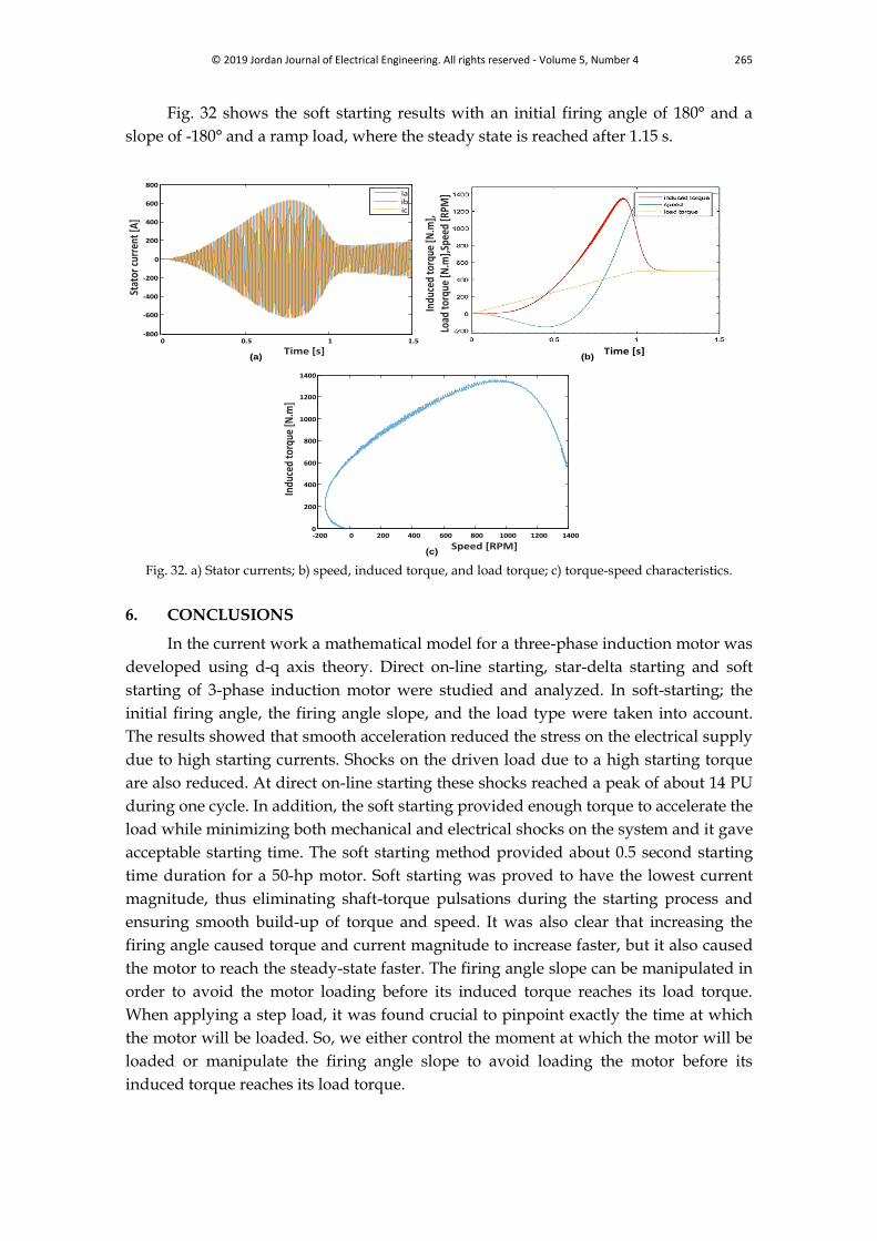
Fig. 32 shows the soft starting results with an initial firing angle of 180° and a
slope of -180° and a ramp load, where the steady state is reached after 1.15 s.
-200 0 200 400 600 800 1000 1200 14000
200
400
600
800
1000
1200
1400
Speed [RPM]
Indu
ced
torq
ue [N
.m]
Time [s]
Indu
ced
torq
ue [N
.m],
Load
torq
ue [N
.m],S
peed
[RPM
]
0 0.5 1 1.5-800
-600
-400
-200
0
200
400
600
800
Time [s]
Stat
or c
urre
nt [A
]
iaibic
(a) (b)
(c) Fig. 32. a) Stator currents; b) speed, induced torque, and load torque; c) torque-speed characteristics.
6. CONCLUSIONS
In the current work a mathematical model for a three-phase induction motor was
developed using d-q axis theory. Direct on-line starting, star-delta starting and soft
starting of 3-phase induction motor were studied and analyzed. In soft-starting; the
initial firing angle, the firing angle slope, and the load type were taken into account.
The results showed that smooth acceleration reduced the stress on the electrical supply
due to high starting currents. Shocks on the driven load due to a high starting torque
are also reduced. At direct on-line starting these shocks reached a peak of about 14 PU
during one cycle. In addition, the soft starting provided enough torque to accelerate the
load while minimizing both mechanical and electrical shocks on the system and it gave
acceptable starting time. The soft starting method provided about 0.5 second starting
time duration for a 50-hp motor. Soft starting was proved to have the lowest current
magnitude, thus eliminating shaft-torque pulsations during the starting process and
ensuring smooth build-up of torque and speed. It was also clear that increasing the
firing angle caused torque and current magnitude to increase faster, but it also caused
the motor to reach the steady-state faster. The firing angle slope can be manipulated in
order to avoid the motor loading before its induced torque reaches its load torque.
When applying a step load, it was found crucial to pinpoint exactly the time at which
the motor will be loaded. So, we either control the moment at which the motor will be
loaded or manipulate the firing angle slope to avoid loading the motor before its
induced torque reaches its load torque.
266 © 2019 Jordan Journal of Electrical Engineering. All rights reserved - Volume 5, Number 4
REFERENCES
[1] A. Bellure, M. Aspalli, "Dynamic d-q model of induction motor using simulink," International
Journal of Engineering Trends and Technology, vol. 24, no. 5, pp. 252-257, 2015.
[2] S. Shah, A. Rashid, M. Bhatti, "Direct quadrate (d-q) modeling of 3-phase induction motor
using matlab/simulink," Canadian Journal on Electrical and Electronics Engineering, vol. 3, no. 5,
pp. 237-243, 2012.
[3] O. Barbarawi, A. Al-Rawashdeh, G. Qaryouti, "Simulink modelling of the transient cases of
three phase induction motors," International Journal of Electrical and Computer Sciences,
vol. 17, no. 04, pp. 6-15, 2018.
[4] O. Momoh, "Dynamic simulation of squirrel cage induction machine- a simplified and
modular approach," International Journal of Engineering Research and Technology, vol. 2, no. 11,
pp. 2307-2313, 2013.
[5] M. Salahat, O. Barbarawe, M. AbuZalata, S. Asad, "Modular approach for investigation of
the dynamic behavior of three-phase induction machine at load variation," Engineering,
vol. 3, pp. 525-531, 2011.
[6] K. Sandhu, V. Pahwa, "Simulation study of three phase induction motor with variations in
moment of inertia," ARPN Journal of Engineering and Applied Sciences, vol. 4, no. 6, pp. 72-77,
2009.
[7] A. Eltamaly, A. Alolah, R. Hamouda, "Performance evaluation of three phase induction
motor under different ac voltage control strategies’ Part I’," 2007 International Aegean
Conference on Electrical Machines and Power Electronics, pp. 770-774, 2007.
[8] S. Ganar, O. Jodh, G. Gulhane, "Implementation of soft starter using 3 phase induction
motor," International Journal of Science and Research, 2017.
[9] I. Boldea, S. Nasar, Electric Drives, Florida: CRC Press, 1998.
[10] C. Obeta, C. Mgbachi, I. Udeh, "Soft starter an alternative to motor control," IJSAR Journal
of Engineering and Computing, vol. 2, no. 1, pp. 9-16, 2015.
[11] T. Wildi, Electrical Machines, Drives, and power systems, Pearson, 5th edition, 2014.
[12] A. Trzyadlowski, Control of Induction Motors, Salt Lake City: Academic press Co., 2001.
[13] C. Naxnin, Z. Qingfan, The application of the fuzzy control technology in intelligent soft start,
PhD Thesis, Shandong University, 2012.
[14] A. Sharma, "Simulation of three phase soft starter using multiple SCRs," International Journal
of Engineering Trends and Technology, vol. 49, no. 7, pp. 451-456, 2017.
[15] B. Trivedi, J. Raval, J. Desai, K. Sonwane, "Soft start of induction motor using TRIAC
switching," International Journal of Engineering Development and Research, vol. 5, no. 2, pp.
1635-1639, 2017.
[16] S. Akshaykumar, T. Sagar, S. Vijay, P. Mone, "Soft starting of three phase induction motor,"
International Journal for Research Trends and Innovation, vol. 2, no. 5, pp. 1-2, 2017.
[17] A. Menaem, A. Amin, "A proposed soft starting technique for three-phase induction motor
using ANN," 16-th International Middle-East Power Systems Conference, 2014.