A Solution Approach for Optimizing Long- and Short-termProduction Scheduling at LKAB’s Kiruna Mine

Michael A. Martinez† • Alexandra M. Newman‡†Department of Mathematical Sciences, United States Air Force Academy, USAF Academy, CO 80840

‡Division of Economics and Business, Colorado School of Mines, Golden, CO 80401michael.martinez@usafa.edu • newman@mines.edu

27 October, 2010

Abstract

We present a mixed-integer program to schedule long- and short-term production at LKAB’sKiruna mine, an underground sublevel caving mine located in northern Sweden. The model min-imizes deviations from monthly preplanned production quantities while adhering to operationalconstraints. Because of the mathematical structure of the model and its moderately large size,instances spanning a time horizon of more than a year or two tend to be intractable. We developan optimization-based decomposition heuristic that, on average, obtains better solutions fasterthan solving the model directly. We show that for realistic data sets, we can generate solutionswith deviations that comprise about 3%-6% of total demand in about a third of an hour.

Keywords:Mining/metals industries: determining optimal operating policies at an underground mineProduction/scheduling applications: production scheduling at an underground mineInteger programming applications: determining a production schedule

1 Introduction

LKAB’s Kiruna iron ore mine, located in northern Sweden, satisfies contracts with its customers for three

different ore grades, B1, B2, and D3. Geological samples predict the locations in the mine at which the

corresponding ore grades are found. Correspondingly, we wish to determine the extraction dates of various

predetermined sections of ore which can contain any amount of the three ore grades and waste. Due to

company policy, the mine holds no inventory; as such, overproduction of any ore grade leads to abandonment

of that ore, while underproduction leads to loss of customer goodwill. Therefore, the mine’s objective is to

meet preplanned monthly targets for each ore grade as closely as possible. The rules according to which

ore is extracted correspond to those of Kiruna’s mining method, an underground method known as sublevel

caving.

In earlier work, Newman et al. (2007) present the problem as a mixed integer linear program. However,

because of the mine size and the time horizon over which planners are interested in obtaining extraction

sequences, the associated model instances are difficult to solve quickly. In this paper, our contribution lies in

showing how we can increase the tractability of that model, specifically, by: (i) eliminating variables without

sacrificing optimality, and then (ii) developing an optimization-based decomposition heuristic to plan ore

extraction sequences for this large, highly automated mine.

1

Using our formulation that incorporates both short- and long-term production scheduling decisions to

meet contractual agreements not only far surpasses any manual methods previously used to schedule iron

ore production at this mine, but also substantially reduces deviations from the contractual agreements when

compared to the schedules obtained from the long-term model in use at the mine at the time of this writing.

Furthermore, we show how we are able to mitigate the long solution times from our more detailed model to

obtain good schedules with about 20 minutes of computation time using real data from the mine; problem

instances span a 30- to 42-month time horizon and possess monthly fidelity. Our decomposition heuristic

exploits problem structure in a novel fashion that could be used on other, similar models (see Section 8).

This paper is organized as follows: Section 2 describes the Kiruna mine, giving details necessary to

understand the formulation. In Section 3, we review relevant literature and differentiate our problem from

existing mine scheduling models. We present our model, that given in Newman et al. (2007), in Section 4.

Sections 5, 6, and 7 represent our contributions in this paper: an explanation of the two ways in which we

expedite solution time, i.e., (i) by eliminating variables (an exact method) and (ii) via the decomposition

procedure (a heuristic method), and a demonstration of the performance of (i) and (ii) against standard

commercial integer programming software. Section 8 concludes the paper.

2 Background

There are about five principal, commonly-used underground mining techniques. The underground mining

technique used depends, inter alia, on the position of the orebody, its composition, and the characteristics,

e.g, softness or hardness, of the orebody and surrounding rock. Because Kiruna is a relatively pure, veinlike

deposit with stable surrounding rock that caves in a controlled fashion when blasted, a method called

sublevel caving can be employed. Open pit mining and underground mining techniques such as block caving

are used more prevalently than sublevel caving. However, the latter technique is nonetheless an important

underground mining method used most commonly at mines in Sweden, Canada, and Australia. In each of

these countries, several million tons of material are produced annually via sublevel caving. Specifically, the

method is used at two different iron ore mines in Sweden, at copper and diamond mines in Canada, and

at various poly-metallic (copper, silver, gold, nickel) mines in Australia. The method has also been used

recently in copper mines in Zambia and is seeing increasing use at an iron ore mine in China. The Kiruna

mine itself is one of the principal suppliers of iron ore to the European steel industry.

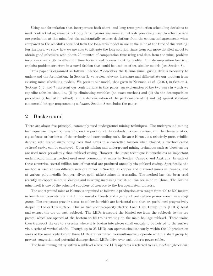
The underground mine at Kiruna is organized as follows: a production area ranges from 400 to 500 meters

in length and consists of about 10 horizontal sublevels and a group of vertical ore passes known as a shaft

group. The ore passes provide access to sublevels, which are horizontal cuts that are positioned progressively

deeper in the earth’s surface. One or two 25-ton-capacity electric Load Haul Dump units (LHDs) blast

and extract the ore on each sublevel. The LHDs transport the blasted ore from the sublevels to the ore

passes, which are opened at the bottom to fill trains waiting on the main haulage sublevel. These trains

then transport the ore to a crusher where it is broken into pieces small enough to be hoisted to the surface

via a series of vertical shafts. Though up to 25 LHDs can operate simultaneously within the 10 production

areas of the mine, only two or three LHDs are permitted to simultaneously operate within a shaft group to

prevent congestion and potential damage should LHDs drive over each other’s power cables.

The basic mining entity within a sublevel where one LHD operates is referred to as a machine placement.

2

A machine placement contains between one and three million tons of ore and waste rock and belongs to a

unique shaft group. Once an LHD starts to mine a machine placement, the machine placement must be

continuously mined until all the ore has been extracted from the machine placement. This restriction prevents

mining crews from having to replace old explosives and schedulers from having to account for partially-mined

machine placements. Preparation crew availability limits the number of machine placements that can be

started each month. Also, LHD availability restricts the number of active machine placements, i.e., machine

placements currently being mined, at any one time.

Sublevel caving operational policies dictate whether machine placements can, or must, be mined de-

pending on the relative position of other machine placements that have started to be mined. Specifically,

a machine placement beneath a given machine placement cannot start to be mined until some portion of

the given machine placement has been mined. Additionally, in order to prevent blast damage in the vicin-

ity, machine placements to the right and left of a given machine placement must start to be mined after a

specified portion of the given machine placement has been mined. Typically, these portions are 50%. These

operational constraints are referred to as vertical and horizontal sequencing constraints, respectively.

For currently active machine placements, the model considers each at a finer level of detail. Specifically,

each active machine placement is modeled as containing between five and fifteen smaller (100 meter-long)

entities known as production blocks. Each production block corresponds to the quantity of ore that an LHD

can mine continuously in a month. Minimum and maximum production rates per month ensure continuous

mining of machine placements, as discussed above, as well as adherence to production capacity restrictions.

Because these machine placements are currently active, because of the number of production blocks each

active machine placement contains, and because of minimum mining rates, for the scenarios we consider, all

production blocks, and, hence, all currently-active machine placements, will finish being mined within two

years, at most.

Several adjacent production blocks form a notional drawdown line within a machine placement. A series

of drawdown lines regulates the order in which production blocks must be mined when executing the sublevel

caving method. Drawdown lines lie horizontally or at a 45 degree angle through several production blocks

within a machine placement. Operational constraints dictate that production blocks in a drawdown line

underneath a given drawdown line cannot be extracted until all ore in the given drawdown line is extracted.

This mining pattern is necessary so that the mined out areas do not collapse on top of ore that has yet

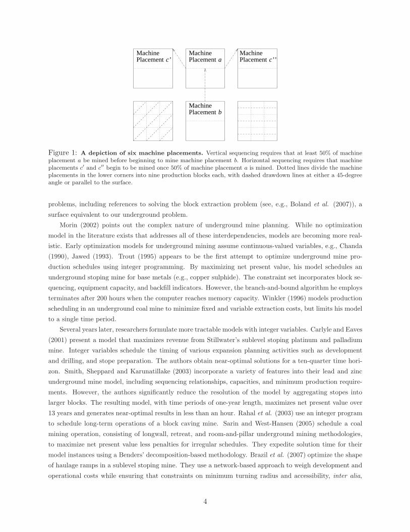
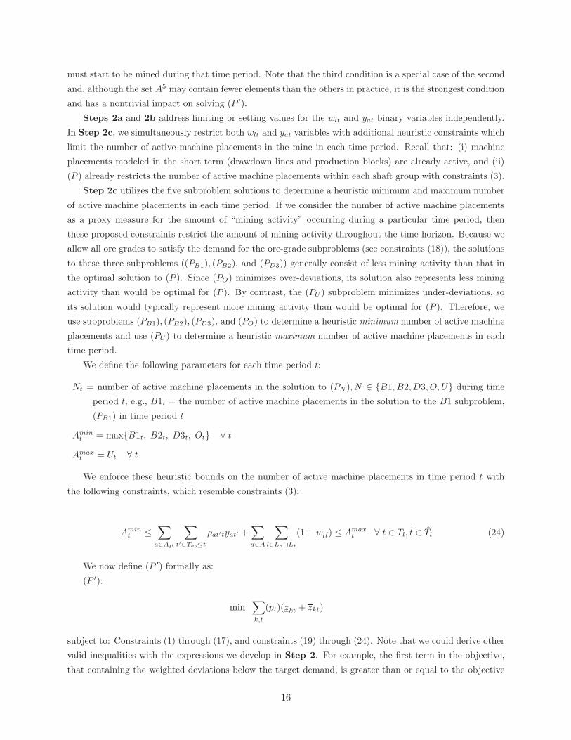
to be retrieved. We illustrate the sequencing constraints and relationships between machine placements,

drawdown lines, and production blocks in Figure 1.

3 Literature Review

The underground mining method known as a sublevel caving possesses a specific set of operational constraints.

In general, these constraints tend to make the problem more complicated than many studied in the surface

mining literature where the earliest applications of mathematical programming in the mining industry lie.

The interested reader can find examples of open pit mining problems, specifically, the ultimate pit limit

problem, or the problem of determining the (time-invariant) envelope of profitable material to extract from

a surface mine in, e.g., Lerchs and Grossman (1965) and Hochbaum and Chen (2000). Recent survey papers

by Frimpong (2002), Osanloo et al. (2008) and Caccetta (2007) provide more examples of surface mining

3

Machine Machine

Machine

Placement Placement

Placement

c’ a

b

Placement c’’Machine

Figure 1: A depiction of six machine placements. Vertical sequencing requires that at least 50% of machineplacement a be mined before beginning to mine machine placement b. Horizontal sequencing requires that machineplacements c

′ and c′′ begin to be mined once 50% of machine placement a is mined. Dotted lines divide the machine

placements in the lower corners into nine production blocks each, with dashed drawdown lines at either a 45-degreeangle or parallel to the surface.

problems, including references to solving the block extraction problem (see, e.g., Boland et al. (2007)), a

surface equivalent to our underground problem.

Morin (2002) points out the complex nature of underground mine planning. While no optimization

model in the literature exists that addresses all of these interdependencies, models are becoming more real-

istic. Early optimization models for underground mining assume continuous-valued variables, e.g., Chanda

(1990), Jawed (1993). Trout (1995) appears to be the first attempt to optimize underground mine pro-

duction schedules using integer programming. By maximizing net present value, his model schedules an

underground stoping mine for base metals (e.g., copper sulphide). The constraint set incorporates block se-

quencing, equipment capacity, and backfill indicators. However, the branch-and-bound algorithm he employs

terminates after 200 hours when the computer reaches memory capacity. Winkler (1996) models production

scheduling in an underground coal mine to minimize fixed and variable extraction costs, but limits his model

to a single time period.

Several years later, researchers formulate more tractable models with integer variables. Carlyle and Eaves

(2001) present a model that maximizes revenue from Stillwater’s sublevel stoping platinum and palladium

mine. Integer variables schedule the timing of various expansion planning activities such as development

and drilling, and stope preparation. The authors obtain near-optimal solutions for a ten-quarter time hori-

zon. Smith, Sheppard and Karunatillake (2003) incorporate a variety of features into their lead and zinc

underground mine model, including sequencing relationships, capacities, and minimum production require-

ments. However, the authors significantly reduce the resolution of the model by aggregating stopes into

larger blocks. The resulting model, with time periods of one-year length, maximizes net present value over

13 years and generates near-optimal results in less than an hour. Rahal et al. (2003) use an integer program

to schedule long-term operations of a block caving mine. Sarin and West-Hansen (2005) schedule a coal

mining operation, consisting of longwall, retreat, and room-and-pillar underground mining methodologies,

to maximize net present value less penalties for irregular schedules. They expedite solution time for their

model instances using a Benders’ decomposition-based methodology. Brazil et al. (2007) optimize the shape

of haulage ramps in a sublevel stoping mine. They use a network-based approach to weigh development and

operational costs while ensuring that constraints on minimum turning radius and accessibility, inter alia,

4

are adhered to. None of the previous examples addresses sublevel caving, which consists of fundamentally

different operational constraints. We refer the interested reader to a survey paper, Alford et al. (2007), that

mentions these and other, related articles, though none, other than a subset of those we cite below, refer to

the sublevel caving technique, our method of interest.

Successive efforts at production scheduling for the Kiruna mine have sought a schedule of requisite length

and resolution in a reasonable amount of solution time. Using the machine placement as the basic mining

unit, Almgren (1994) considers a one-month time frame; hence, in order to generate a five-year schedule, he

runs the model 60 times. In a similar vein, Topal (1998) and Dagdelen, Kuchta and Topal (2002) iteratively

solve one-year subproblems (with monthly resolution) in order to achieve production plans for five-year and

seven-year time horizons, respectively. Kuchta, Newman and Topal (2004) also consider Kiruna’s decisions at

the machine placement level. The authors improve model tractability by modifying earlier formulations and

eliminating some decision variables. Their model instances consist of a five-year time horizon and three ore

grades, which they are able to solve to near-optimality in a matter of minutes. Newman and Kuchta (2007)

improve tractability of the model presented in Kuchta, Newman and Topal (2004) using an optimization-

based heuristic consisting of deriving information from a faster-solving aggregated model to guide the search

in the original model. Newman et al. (2007) present a more detailed model of the same mine in which

decisions are made both at the machine placement level, and at a finer level, the production block level. The

authors show how using such a model yields schedules that more closely align production and demanded

quantities for all ore grades and time periods. Specifically, the combined resolution model reduces total

absolute deviations from planned production quantities by approximately 70% over those obtained from the

model with only long-term resolution. However, the paper presents model instances that are only solvable

in their monolithic form. Such instances possess time horizons of two years or fewer.

Our contribution lies in developing a heuristic to aid in the solution of model instances for the formulation

that Newman et al. (2007) present. To our knowledge, such a detailed model for underground sublevel caving

operations, or for similar production scheduling operations, exists only as presented in the afore-mentioned

reference, and no attention has yet been given to solving such a model for horizons longer than two years,

or, generally, for model instances that are not solvable directly, i.e., in their monolithic form. Furthermore,

our decomposition heuristic contains a variety of novel characteristics which we are able to exploit based on

the mathematical structure of the model.

4 Model

The long-term model in use at the Kiruna mine at the time of this writing (Kuchta, Newman and Topal, 2004)

determines which machine placements to start mining in each time period over the horizon to minimize de-

viations from planned production quantities while considering vertical and horizontal sequencing constraints

and restrictions on the allowable number of LHDs in each shaft group. We refer to this optimization model

as the long-term model.

The model given in Newman et al. (2007) consists both of long-term decisions and restrictions coupled

with corresponding short-term characteristics. The latter element allows the model to more closely control

the amount and grades of ore that are extracted from each machine placement in the near term. Continuous-

valued variables track the amount mined in each production block and time period while binary variables

5

represent whether or not all production blocks contained in a given drawdown line have finished being mined

by a given time period.

Accordingly, we add the following types of constraints to the long-term model: (i) those that limit the

amount extracted from a production block to the reserves available within that production block; (ii) those

that indicate when a drawdown line has finished being mined; (iii) those that prevent production blocks in an

underlying drawdown line from being mined until those in the overlying drawdown line have been completely

extracted; (iv) those that capture vertical and horizontal sequencing between production blocks, drawdown

lines, and machine placements; (v) those that regulate both minimum and maximum monthly production

rates; and (vi) those that enforce demand constraints for the first few time periods of the horizon.

A complete mathematical formulation of the combined (short- and long-term) model follows. This is

a slightly more detailed formulation than that appearing in Newman et al. (2007); although the model

is identical, we restate it here for the reader’s convenience. Owing to space considerations, we define all

indices in the definitions of the sets, parameters, and variables. It is understood that any index with a prime

represents an alias of that index, e.g., t and t′ are both indices of time.

SETS:

K = set of ore grades

V = set of shaft groups

A = set of machine placements

Av = set of machine placements in shaft group v

IA = set of inactive machine placements

AVa = set of machine placements whose start date is restricted vertically by machine placement a

AHa = set of machine placements whose start date is forced by adjacency to machine placement a

At = set of machine placements that can start to be mined in time period t

B = set of production blocks

Ba = set of production blocks in machine placement a

Bl = set of production blocks in drawdown line l

Bt = set of production blocks that can be mined in time period t

L = set of drawdown lines

La = last (i.e., most deeply positioned) drawdown line in machine placement a

LC = set of drawdown lines constrained by another drawdown line

Ll = set of drawdown lines that vertically constrain drawdown line l

LVa = drawdown line whose finish date vertically restricts starting to mine machine placement a

LHa = drawdown line whose finish date forces the start date of machine placement a by adjacency

Lt = set of drawdown lines that can be mined in time period t

6

T = set of time periods composing the long-term time horizon (T is the complement thereof)

T = set of time periods composing the short-term time horizon (⊂ T )

Ta = set of time periods in which machine placement a can start to be mined (restricted by machine

placement location and the start dates of other relevant machine placements)

Tb = set of time periods in which production block b can be mined (restricted by production block location

and the start dates of other relevant production blocks)

Tl = set of time periods in which drawdown line l can finish being mined (restricted by drawdown line

location and the finish times of other relevant drawdown lines)

Tl = time period by which all production blocks in drawdown line l must finish being mined

PARAMETERS:

pt = penalty associated with deviations in time period t (= |T |+ 1− t)

LHD t = maximum number of machine placements that can start to be mined in time period t

LHDv = maximum number of active machine placements in shaft group v

dkt = target demand for ore grade k in time period t (ktons)

rat′tk = reserves of ore grade k available at time t in machine placement a given that the machine placement

started to be mined at time t′ (ktons)

ρat′t =

{

1 if machine placement a started to be mined at t′ and is being mined at time t

0 otherwise

Rbk = reserves of ore grade k contained in production block b (ktons)

Cat = minimum production rate of machine placement a in time period t (ktons per time period)

Cat = maximum production rate of machine placement a in time period t (ktons per time period)

DECISION VARIABLES:

zkt = deviation above the target demand for ore grade k in time period t (ktons)

zkt = deviation below the target demand for ore grade k in time period t (ktons)

xbt = amount of ore mined from production block b in time period t (ktons)

wlt =

1 if we finish mining all production blocks contained in drawdown line l

by time period t

0 otherwise

yat =

{

1 if we start mining machine placement a at time period t

0 otherwise

7

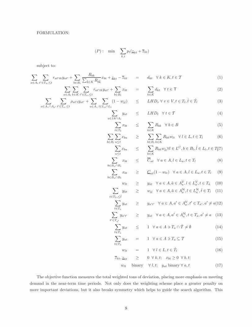
FORMULATION:

(P ) : min∑

k,t

pt(zkt + zkt)

subject to:

∑

a∈At

∑

t′∈Ta,≤t

rat′tkyat′ +∑

b∈Bt

Rbk∑

k∈KR

bk

xbt + zkt − zkt = dkt ∀ k ∈ K, t ∈ T (1)

∑

a∈At

∑

k∈K

∑

t′∈Ta,≤t

rat′tkyat′ +∑

b∈Bt

xbt =∑

k∈K

dkt ∀ t ∈ T (2)

∑

a∈Av∩At′

∑

t′∈Ta,≤t

ρat′tyat′ +∑

a∈Av

∑

l∈La∩Lt

(1− wlt) ≤ LHDv ∀ v ∈ V, t ∈ Tl, t ∈ Tl (3)

∑

a∈IA∩At

yat ≤ LHDt ∀ t ∈ T (4)

∑

t∈Tb

xbt ≤∑

k∈K

Rbk ∀ b ∈ B (5)

∑

b∈Bl

∑

u≤t

xbu ≥∑

b∈Bl

∑

k∈K

Rbkwlt ∀ l ∈ L, t ∈ Tl (6)

∑

u≤t

xbu ≤∑

k∈K

Rbkwlt∀l ∈ LC , b ∈ Bl, l ∈ Ll, t ∈ T

l(7)

∑

b∈Ba∩Bt

xbt ≤ Cat ∀ a ∈ A, l ∈ La, t ∈ Tl (8)

∑

b∈Ba∩Bt

xbt ≥ Cat(1− wlt) ∀ a ∈ A, l ∈ La, t ∈ Tl (9)

wlt ≥ yat ∀ a ∈ A, a ∈ AVa , l ∈ LV

a , t ∈ Ta (10)∑

t∈Ta,≤t

yat ≥ wlt ∀ a ∈ A, a ∈ AHa , l ∈ LH

a , t ∈ Tl (11)

∑

t∈Ta

yat ≥ ya′t′ ∀ a ∈ A, a′ ∈ AVa , t′ ∈ Ta′ , a′ 6= a(12)

∑

t′∈Ta′

ya′t′ ≥ yat ∀ a ∈ A, a′ ∈ AHa , t ∈ Ta, a

′ 6= a (13)

∑

t∈Ta

yat ≤ 1 ∀ a ∈ A ∋ Ta ∩ T 6= ∅ (14)

∑

t∈Ta

yat = 1 ∀ a ∈ A ∋ Ta ⊆ T (15)

wlt = 1 ∀ l ∈ L, t ∈ Tl (16)

zkt, zkt ≥ 0 ∀ k, t; xbt ≥ 0 ∀ b, t;

wlt binary ∀ l, t; yat binary ∀ a, t (17)

The objective function measures the total weighted tons of deviation, placing more emphasis on meeting

demand in the near-term time periods. Not only does the weighting scheme place a greater penalty on

more important deviations, but it also breaks symmetry which helps to guide the search algorithm. This

8

weighting scheme could also account for ore grade, k; however, as the objective function variables, zkt and

zkt, are continuous, the effect of breaking symmetry in more than one way would have little effect on model

tractability. Because the number of time periods greatly outnumbers the number of ore grades in our model

instances, we choose only to differentiate penalty coefficients by the former characteristic. We use the L-

1 norm to be consistent with the long-term schedules, see, e.g., Kuchta, Newman and Topal (2004), and

also because our penalty term in the objective captures the company’s goals, i.e., to minimize deviations

in the short term over those in the longer term. With this weighting scheme for the penalties, the early

contributions to the total weighted deviation are somewhat higher, especially in the first ten periods, because

of initial conditions, i.e., currently active machines placements that are not part of a solution to an earlier

optimization model! Additionally, although linear integer solvers such as CPLEX can handle models with

(convex) quadratic objectives, e.g., the L-2 norm construct, such solvers tend to be more effective on purely

linear integer models because many model instance tightening tactics do not apply in any type of nonlinear

integer setting and hence, even integer models with simple nonlinearities may be more difficult to solve than

their linear counterparts (Klotz, 2010).

Note that we omit an explicit consideration of cost in the objective function which reflects Kiruna’s

operational policy. This policy is the result of the difference between the markets for iron ore and precious

metals. Precious metals such as gold and silver are traded on, for example, the Commodity Exchange of New

York. These metals are bought and sold worldwide, and the strategy of mines extracting these metals is to

maximize profits by producing as much as is economically viable given current market prices. By contrast,

markets associated with base metals such as iron ore are regionalized, as transportation costs are high relative

to the value of the commodity. Within these markets, steel companies enter into a contract with an iron

ore producer, settling on a price commensurate with the chemical and physical characteristics of the iron

ore. Large buyers tend to influence prices in contracts between other buyers and iron ore producers. The

negotiated prices generally hold for about a year, and iron ore producers are obligated to supply a certain

amount of ore to each buyer with whom they hold a contract. Therefore, iron ore mines like Kiruna are

concerned with meeting contractual demands as closely as possible.

Constraints (1) record for each ore grade and time period the amount in excess or short of the target

demand of ore production. The first term on the left hand side of the constraint records the amount

of ore recovered from machine placements, while the second term records the amount of ore retrieved from

production blocks. Constraints (2) require that for each time period in the short term (typically, six months),

the target amount of ore, regardless of grade, is mined. This requirement prevents the post-processing mills

from sitting idle. Constraints (3) limit the maximum number of active machine placements in each shaft

group and time period. Constraints (4) restrict the number of long-term machine placements that can be

started in a time period; short-term machine placements are assumed to be currently active. Constraints

(5) preclude mining more than the available reserves within a production block. Constraints (6) relate

finishing mining a drawdown line to finishing mining the production blocks within that drawdown line.

Constraints (7) preclude a production block in a drawdown line from starting to be mined until all blocks

in constraining drawdown lines have been mined. Constraints (8) and (9) enforce monthly maximum and

minimum production rates, respectively. Because these rate constraints only apply to the machine placement

as a whole, rather than to each production block, we enforce them with respect to the last drawdown line,

i.e., place at which the machine placement finishes when modeled with production blocks. Constraints

9

(10) and (11) enforce vertical and horizontal sequencing, respectively, between machine placements modeled

with short-term and long-term resolution. Note that the drawdown line in a machine placement modeled

with short-term resolution both (i) controls access (vertically) to a constrained machine placement modeled

with long-term resolution, and (ii) forces mining (horizontally) a machine placement modeled with long-

term resolution. Constraints (12) and (13) enforce vertical and horizontal sequencing, respectively, between

machine placements modeled with long-term resolution. Note that with the appropriate sets of machine

placements in AVa and AH

a , these constraints enforce the 50% rule discussed in Section 1. Constraints (14)

prevent a machine placement from being mined more than once in the horizon, while constraints (15) are a

special case of the former constraint and require a machine placement to be mined exactly once during the

horizon if its eligible start dates fall entirely within the model’s planning horizon. Constraints (16) ensure

that a drawdown line has finished being mined by its last eligible time period. Finally, constraints (17)

enforce non-negativity and integrality, as appropriate.

5 Variable Elimination

Recall that our contribution in this paper lies not in defining the problem, but in posing techniques to

expedite the solution time for realistic problem instances. After showing that instances of (P ) are NP-hard,

we propose two different techniques to expedite solution time: (i) variable elimination, an exact technique,

and (ii) problem decomposition, a heuristic. We describe the former technique in this section.

Instances of (P ) are NP-hard. Consider the following three simplifications of the problem: (i) it requires

only one time period to mine a machine placement, (ii) we examine only one ore grade, and (iii) demand is

constant for all time periods. Then constraints (2) simplify to:∑

a∈Atrayat ≤ d ∀t, and, together with

(15),∑

t∈Tayat = 1 ∀ a ∈ A ∋ Ta ⊆ T , constitute the bin-packing problem. In this case, the a index

corresponds to the item index, the number of items is the cardinality of the set to which the elements a

belong, the size of each item is ra, and the t index corresponds to bins. Because the bin packing problem

is NP-complete (Garey and Johnson, 1979, p. 226), we can conclude that our problem is at least as hard.

Empirically, model instances relevant to our study contain at least a thousand binary variables and 2000 to

3000 constraints.

Rather than retain all |A| × |T | binary yat variables, we can reduce the number of integer variables by

assigning an earliest possible start date to each machine placement. Assigning early start dates is similar to

finding an activity’s earliest start time using a Critical Path Model (CPM) (see, e.g., Rardin, 1998, Section

9.7) applied to a directed, acyclic network. Each node, with the exception of the source and the sink node,

represents a machine placement. Nodes i and j are connected via arc (i, j) based on vertical sequencing

constraints that dictate precedence relationships between mining machine placements; arcs connect nodes

based on the 50% rule, i.e., once 50% of machine placement i is mined out, machine placement j can start to

be mined. The cost on arc (i, j) represents the duration of time machine placement i must be mined before

machine placement j can start to be mined. Without considering additional model constraints, the longest

path in this network between the source node and node i would correspond to the earliest start time for

machine placement i. However, we must also consider the interactions between machine placements other

than simple precedence restrictions (i.e., other than the vertical sequencing constraints). The horizontal

sequencing constraints are, in essence, “forcing” constraints that require, rather than allow, a subsequent

10

activity to be started after a given activity has started (or has been completed). Additionally, our model

limits the number of machine placements that can simultaneously be mined due to LHD availability. This

resource constraint restricts the number of simultaneously-mined machine placements. These two additional

requirements beyond those of the CPM preclude us from simply solving a network problem to determine

early start dates. Instead, we develop a customized algorithm to take these additional restrictions into

consideration. We present this algorithm in the Appendix.

Models in the literature present integer programming formulations for critical path models with resource

constraints, and devise solution procedures for these problems. For example, Demeulemeester and Herroelen

(1992) minimize project duration subject to precedence and resource constraints using a branch-and-bound

procedure with precedence rules to fathom major portions of the branch-and-bound tree. Nudtasomboon and

Randhawa (1997) extend Talbot’s (1982) implicit enumeration methodology to account for objectives other

than minimizing makespan. Others, e.g., Minciardi, Paolucci and Puliafito (1994), Padman, Smith-Daniels

and Smith-Daniels (1997), develop heuristic procedures to determine solutions to the resource-constrained

project scheduling problem. Golenko-Ginzburg and Gonik (1997) examine stochastic project scheduling

with limited resources, and provide a rigorous list of references on deterministic project scheduling. Our

algorithms differ from those presented in these papers in approach, application, and purpose – we use the

results of these algorithms not as an end in and of itself, but to reduce the size of our monolithic (original)

model.

We can construct an algorithm, similar to the early start algorithm, to assign a late start date to each

machine placement. This late start date would eliminate decisions to start to mine a machine placement

so late that adjacent and underlying machine placements eventually become “locked in,” thereby increasing

the amount of deviation between the actual and the planned production quantities beyond values otherwise

obtained in an optimal solution. Assigning late start dates bears similarity to determining the latest time

an activity can start using a backward pass on a CPM. However, in addition to the operational constraints

mentioned in the case of early start dates that cannot be handled on a pure CPM network, we face another

difficulty. To compute latest start dates, the project’s due date, as well as the duration of each activity and

the precedence relationships between each activity, must be known. In our case, the due date corresponds to

the time at which a certain amount of demand must be met. However, our objective is to minimize deviations

from planned production quantities. Without knowing, a priori, that the optimal objective function value

equals zero (which is usually not the case!), we cannot set late start dates based on satisfying all demand.

We can, however, use information about active machine placements together with horizontal sequencing

constraints to determine the latest time period in which a subset of machine placements can start to be

mined. Specifically, for any machine placement whose start date is affected by an active machine placement,

we can assign a latest start date based on the rule that as soon as a certain percentage of the active machine

placement is mined, the affected machine placement must start to be mined to prevent blast damage. Then,

in turn, we can assign late start dates to machine placements whose start dates are affected by machine

placements with late start dates. Topal (2008) addresses some of these issues.

We can also eliminate variables associated with mining a drawdown line before an earliest finish date or

after a late finish date, hence creating the set Tl. We can determine an early finish date for a drawdown

line based on the principle of a pure critical path model, i.e., a critical path model without any resource

constraints. We can compare the tonnage available in each drawdown line with the tonnage that can be

11

mined in each time period based on the following information: (i) the maximum or minimum production

rate, (ii) the position at which a given drawdown line lies relative to all other drawdown lines whose position

could affect accessing the given drawdown line, and (iii) the aggregate tonnage of all blocks comprising each

drawdown line. The earliest a given drawdown line can finish being mined is the sum of the following two

terms: (i) time at which the first drawdown line in the machine placement finishes being mined (recall that

because each machine placement is active in the short term, we know when the first drawdown line starts to

be mined), and (ii) the shortest amount of time for all drawdown lines overlying the given drawdown line

to be mined. Similarly, the latest time at which a drawdown line could finish being mined is the time at

which the first drawdown line in the machine placement finishes being mined added to the longest amount

of time it would require for all drawdown lines overlying the given drawdown line to be mined. Then, we

can eliminate any wlt variables corresponding to finishing to mine a drawdown line before its earliest finish

date or after its latest finish date.

Note that we can use similar principles to establish early start and late finish dates for production blocks,

thereby using the set Tb to eliminate xbt variables corresponding to extracting any amount from a production

block before its earliest start date or after its latest finish date. Because the variables associated with mining

a production block are continuous, the direct benefit of eliminating such variables is small. However, an

indirect benefit of an early start date for each production block is its use in establishing an early start date

for a drawdown line, which is simply the earliest early start date among all blocks in a drawdown line. Early

start dates for a drawdown line help to eliminate irrelevant terms in the shaft group constraint, constraint

(3).

6 Decomposition-Based Heuristic

If we attempt to solve realistic instances of (P ) directly, we encounter extremely long solution times, even

using variable elimination techniques (see Section 5). Another difficulty we encounter is our inability to

readily identify feasible solutions, even if they are far from optimal. Such feasible solutions, if available,

could be used along with mixed integer programming algorithmic heuristics, e.g., local search, to obtain

reasonable solutions fairly quickly. However, the sequencing constraints, (10)-(13), are complex, rendering the

identification of such feasible solutions difficult, at best. Indeed, even the long-term sequencing constraints,

(12)-(13), are difficult to satisfy, so much so that experienced long-term planners who used to construct

Kiruna’s schedules manually often found themselves with an infeasible schedule in the middle of their process

and were forced to resequence (see Kuchta, Newman and Topal (2004)). Additionally, our experimentation

with tailored rounding heuristics based on linear programming relaxation solutions failed to produce feasible

integer solutions. Unfortunately, although solvers such as CPLEX have the capability of accepting a partially

feasible solution, the solution repair heuristics contained in such software are, at the time of this writing,

only mildly effective (Klotz, 2010).

Therefore, we introduce another approach to increase model tractability that we use in conjunction

with variable elimination techniques. In this section, we introduce a heuristic. Specifically, we describe an

optimization-based decomposition heuristic that we apply to (P ), the monolith integer program. The goal

of the heuristic procedure, which we label (H), is to achieve near-optimal solutions more quickly than by

solving (P ) directly, i.e., by executing the procedure (P). (Note: The use of the script letter denotes the

12

procedure, while Roman font denotes a problem.) The heuristic involves first solving subproblems of (P ),

and then using information from the subproblem solutions to solve a constrained version of (P ), which we

label (P ′). We expect (P ′) to obtain better solutions more quickly than attempting to solve (P ) directly.

Although executing (H) may eliminate the optimal solution, executing (P) is intractable enough such that

optimal solutions to instances of (P ) cannot be obtained in a realistic amount of time (hours, or possibly

even days). For example, to obtain a solution of our baseline, three-year instance within 5% of optimality,

even after eliminating variables as discussed in Section 5, the time required is in excess of five million seconds,

or approximately 60 days. By contrast, (P ′) contains information which helps to guide the solver to a good

solution. Although we provide no formal proof on the bounds of the solution quality of our heuristic, we

show in Section 7 that the solutions are typically very good.

Instead of using typical (e.g., temporal or spatial) decomposition techniques, our heuristic decomposes

the model with respect to its objective function components. Recall that the objective function of (P )

balances, for each ore grade, both under- and over-deviations. In our decomposition of the objective, we

consider subproblem solutions that are “extreme” cases of the objective function. We formulate a total of

five subproblems, decomposing the objective function either by ore grade or by the nature of the deviation

(i.e., under- vs. over-deviations).

Three subproblems penalize deviations only for a particular ore grade (B1, B2, D3). Additionally, for

each subproblem (Pk), where k ∈ {B1, B2, D3}, we allow all three ore grades to fulfill demand for ore grade

k. We retain all other constraints in (P ). Specifically, we define:

(Pk) : min∑

t

(pt)(zkt + zkt) ∀ k

subject to:

∑

a∈At

∑

t′∈Ta,≤t

∑

k∈K

rat′tkyat′ +∑

b∈Bt

xbt +∑

k

(zkt − zkt) =∑

k∈K

dkt ∀ t ∈ T (18)

and (2) through (17).

Because we assume |K| ore grades, the replacement of constraints (1) with constraints (18) reduces the

number of constraints in constraint set (1) by |K|−1

|K| .

For the other two subproblems in which we penalize either only production overage, (PO), or production

underage, (PU ), the constraint set is identical to that of (P ), but for subproblem (PO), we penalize only

over-deviations in the objective, while we penalize only under-deviations in (PU ). Specifically:

(PO) : min∑

k,t

ptzkt

subject to constraints (1) through (17).

13

(PU ) : min∑

k,t

ptzkt

subject to constraints (1) through (17).

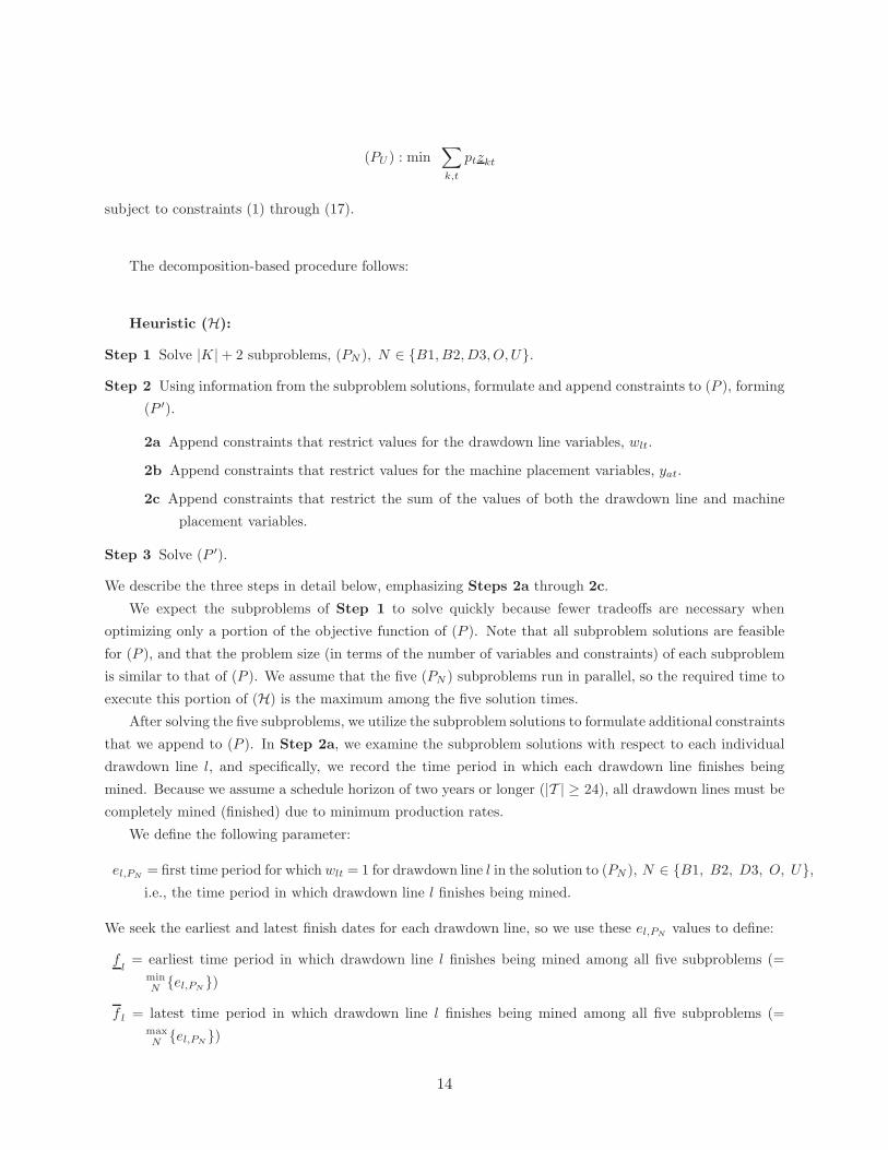
The decomposition-based procedure follows:

Heuristic (H):

Step 1 Solve |K|+ 2 subproblems, (PN ), N ∈ {B1, B2, D3, O, U}.

Step 2 Using information from the subproblem solutions, formulate and append constraints to (P ), forming

(P ′).

2a Append constraints that restrict values for the drawdown line variables, wlt.

2b Append constraints that restrict values for the machine placement variables, yat.

2c Append constraints that restrict the sum of the values of both the drawdown line and machine

placement variables.

Step 3 Solve (P ′).

We describe the three steps in detail below, emphasizing Steps 2a through 2c.

We expect the subproblems of Step 1 to solve quickly because fewer tradeoffs are necessary when

optimizing only a portion of the objective function of (P ). Note that all subproblem solutions are feasible

for (P ), and that the problem size (in terms of the number of variables and constraints) of each subproblem

is similar to that of (P ). We assume that the five (PN ) subproblems run in parallel, so the required time to

execute this portion of (H) is the maximum among the five solution times.

After solving the five subproblems, we utilize the subproblem solutions to formulate additional constraints

that we append to (P ). In Step 2a, we examine the subproblem solutions with respect to each individual

drawdown line l, and specifically, we record the time period in which each drawdown line finishes being

mined. Because we assume a schedule horizon of two years or longer (|T | ≥ 24), all drawdown lines must be

completely mined (finished) due to minimum production rates.

We define the following parameter:

el,PN= first time period for which wlt = 1 for drawdown line l in the solution to (PN ), N ∈ {B1, B2, D3, O, U},

i.e., the time period in which drawdown line l finishes being mined.

We seek the earliest and latest finish dates for each drawdown line, so we use these el,PNvalues to define:

fl

= earliest time period in which drawdown line l finishes being mined among all five subproblems (=min

N{el,PN

})

f l = latest time period in which drawdown line l finishes being mined among all five subproblems (=max

N{el,PN

})

14

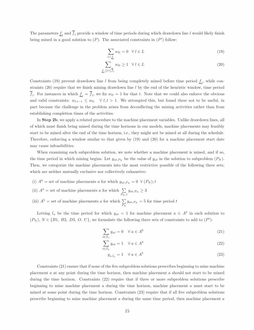
The parameters fland f l provide a window of time periods during which drawdown line l would likely finish

being mined in a good solution to (P ). The associated constraints in (P ′) follow:

∑

t<fl

wlt = 0 ∀ l ∈ L (19)

∑

fl≤t≤f

l

wlt ≥ 1 ∀ l ∈ L (20)

Constraints (19) prevent drawdown line l from being completely mined before time period fl, while con-

straints (20) require that we finish mining drawdown line l by the end of the heuristic window, time period

f l. For instances in which fl

= f l, we fix wlt = 1 for that t. Note that we could also enforce the obvious

and valid constraints: wl,t−1 ≤ wlt ∀ l, t > 1. We attempted this, but found these not to be useful, in

part because the challenge in the problem arises from deconflicting the mining activities rather than from

establishing completion times of the activities.

In Step 2b, we apply a related procedure to the machine placement variables. Unlike drawdown lines, all

of which must finish being mined during the time horizons in our models, machine placements may feasibly

start to be mined after the end of the time horizon, i.e., they might not be mined at all during the schedule.

Therefore, enforcing a window similar to that given by (19) and (20) for a machine placement start date

may cause infeasibilities.

When examining each subproblem solution, we note whether a machine placement is mined, and if so,

the time period in which mining begins. Let yat,PNbe the value of yat in the solution to subproblem (PN ).

Then, we categorize the machine placements into the most restrictive possible of the following three sets,

which are neither mutually exclusive nor collectively exhaustive:

(i) A0 = set of machine placements a for which yat,PN= 0 ∀ (PN ), t

(ii) A3 = set of machine placements a for which∑

PN ,t

yat,PN≥ 3

(iii) A5 = set of machine placements a for which∑

PN

yat,PN= 5 for time period t

Letting ta be the time period for which yat = 1 for machine placement a ∈ A5 in each solution to

(PN ), N ∈ {B1, B2, D3, O, U}, we formulate the following three sets of constraints to add to (P ′):

∑

t∈Ta

yat = 0 ∀ a ∈ A0 (21)

∑

t∈Ta

yat = 1 ∀ a ∈ A3 (22)

ya,ta= 1 ∀ a ∈ A5 (23)

Constraints (21) ensure that if none of the five subproblem solutions prescribes beginning to mine machine

placement a at any point during the time horizon, then machine placement a should not start to be mined

during the time horizon. Constraints (22) require that if three or more subproblem solutions prescribe

beginning to mine machine placement a during the time horizon, machine placement a must start to be

mined at some point during the time horizon. Constraints (23) require that if all five subproblem solutions

prescribe beginning to mine machine placement a during the same time period, then machine placement a

15

must start to be mined during that time period. Note that the third condition is a special case of the second

and, although the set A5 may contain fewer elements than the others in practice, it is the strongest condition

and has a nontrivial impact on solving (P ′).

Steps 2a and 2b address limiting or setting values for the wlt and yat binary variables independently.

In Step 2c, we simultaneously restrict both wlt and yat variables with additional heuristic constraints which

limit the number of active machine placements in the mine in each time period. Recall that: (i) machine

placements modeled in the short term (drawdown lines and production blocks) are already active, and (ii)

(P ) already restricts the number of active machine placements within each shaft group with constraints (3).

Step 2c utilizes the five subproblem solutions to determine a heuristic minimum and maximum number

of active machine placements in each time period. If we consider the number of active machine placements

as a proxy measure for the amount of “mining activity” occurring during a particular time period, then

these proposed constraints restrict the amount of mining activity throughout the time horizon. Because we

allow all ore grades to satisfy the demand for the ore-grade subproblems (see constraints (18)), the solutions

to these three subproblems ((PB1), (PB2), and (PD3)) generally consist of less mining activity than that in

the optimal solution to (P ). Since (PO) minimizes over-deviations, its solution also represents less mining

activity than would be optimal for (P ). By contrast, the (PU ) subproblem minimizes under-deviations, so

its solution would typically represent more mining activity than would be optimal for (P ). Therefore, we

use subproblems (PB1), (PB2), (PD3), and (PO) to determine a heuristic minimum number of active machine

placements and use (PU ) to determine a heuristic maximum number of active machine placements in each

time period.

We define the following parameters for each time period t:

Nt = number of active machine placements in the solution to (PN ), N ∈ {B1, B2, D3, O, U} during time

period t, e.g., B1t = the number of active machine placements in the solution to the B1 subproblem,

(PB1) in time period t

Amint = max{B1t, B2t, D3t, Ot} ∀ t

Amaxt = Ut ∀ t

We enforce these heuristic bounds on the number of active machine placements in time period t with

the following constraints, which resemble constraints (3):

Amint ≤

∑

a∈At′

∑

t′∈Ta,≤t

ρat′tyat′ +∑

a∈A

∑

l∈La∩Lt

(1− wlt) ≤ Amaxt ∀ t ∈ Tl, t ∈ Tl (24)

We now define (P ′) formally as:

(P ′):

min∑

k,t

(pt)(zkt + zkt)

subject to: Constraints (1) through (17), and constraints (19) through (24). Note that we could derive other

valid inequalities with the expressions we develop in Step 2. For example, the first term in the objective,

that containing the weighted deviations below the target demand, is greater than or equal to the objective

16

function value of (PU ) while the second term in the objective is greater than or equal to the objective function

value of (PO). Such constraints, however, are unlikely to improve tractability as they simply place bounds

on sums of continuous, rather than binary, variables.

In Step 3 of (H), we solve (P ′).

The intuition behind the heuristic is as follows: In determining the grade and quantity of ore to extract

in each time period, many tradeoffs must be made between the nature of the deviation, i.e., the ore grade

and underage versus overage. In each subproblem, we allow just one tradeoff to be considered. When

multiple subproblems solved in isolation “agree” either simply on the section of ore to be extracted, or,

more specifically, on the timing of said extraction, implementing a corresponding constraint in the monolith

tends to produce good solutions. Clearly, the fact that we consider the subproblems independently when,

in fact, they are not, does not guarantee through the implementation of these constraints that we produce

an optimal solution. In fact, it is quite possible that a section of ore that appeared favorable for each

independent subproblem is not part of a favorable solution for the monolith. Confounding factors such as

other ore sections that cannot be or are not mined in the monolith but whose mining was necessary for a

good-quality subproblem solution can contribute to suboptimality of this heuristic.

Despite this caveat, we produce good solutions with our heuristic. We demonstrate the quality of our

solutions relative to what the monolith can produce and relative to exact lower bounds in the following

section. A few implementation issues follow: Because all subproblems (PN ) and the constrained version

of (P ), (P ′), remain complex integer programming problems with sizes comparable to (P ), we sometimes

impose time and/or solution quality limits when executing (H). Specifically, for both (PU ) and (PD3), we

impose both a time limit and a solution quality limit of the form min{250 seconds, 1% optimality gap}

because the deviations these subproblems minimize typically constitute the majority of the deviations in

optimal schedules for (P ). Among other reasons, this characteristic seems to contribute to the difficulty

in solving these subproblems, and to weak lower bounds. If these subproblems are run to optimality, their

solutions may slightly alter specific constraints we generate in (H), Step 2; however, when using optimal

solutions in practice, we realize insufficient improvements in the solution to (P ′) to justify the long run time.

From empirical analysis of several lengthy (P ′) runs (e.g., 3000 seconds or more), we notice that almost

all of the improvement (typically, about 95%) in the objective function is made in the first 750 seconds.

Because we set the solver parameters to aggressively seek an optimal solution, we expect improvement in

the objective function value to diminish over time. Therefore, we set a time limit of 750 seconds when

solving (P ′). Typically, once the solver encounters a near-optimal solution, it spends a high percentage of

the remaining solution time improving the lower bound.

7 Computational Results

We present computational results from implementing heuristic (H) described in Section 6 and compare it

using procedure (P), which we consider the default procedure. We conduct all numerical experiments with

the AMPL programming language (Fourer, Gay and Kernighan, 2003; and AMPL Optimization LLC, 2001)

and the CPLEX solver, Version 9.1 (ILOG Corporation, 2005). We execute the timed runs on a Sunblade

1000 computer with 1 GB RAM, while also conducting additional runs calculating lower bounds on a Beowulf

Parallel Cluster with 96 processors and 280 GB of total RAM. We tailor the CPLEX parameter settings to

17

obtain efficient performance both in terms of good integer solutions and in terms of a strong bound for each

of the three problem types: the (PN ) subproblems, (P ′), and (P ). In general, we rely on (i) applying the

relaxation induced neighborhood search heuristic (Danna, Rothberg and Le Pape, 2005), and (ii) altering

the emphasis of the algorithm.

Our baseline scenario possesses current data from LKAB’s Kiruna mine. The data set contains three

ore grades, and spans three years or 36 (monthly) time periods. From this scenario, we perturb the data

set in three ways: (i) changing labor availability, (ii) changing equipment availability, and (iii) changing

ore reserves. In (i) and (ii), we simply rearrange existing mine capacity. As a proxy for perturbing the

ore reserves, we shorten or lengthen the time horizon (from the baseline of three years) by six months,

which alters the ore reserves to which miners have access. We consider each of the three methods of data

perturbation to result in realistic Kiruna scenarios. For each base case with a given time horizon length,

we generate four additional data sets, yielding a total of 15 data sets (3 baseline and 12 simulated) against

which we compare the performance of (H) to using (P).

The size of (P ) is directly related to the length of the time horizon. For the 2.5-year models, the problems

contain approximately 870 binary variables, 650 continuous variables, and 2160 constraints. In general, the

3-year models contain 1100 binary variables, 690 continuous variables, and 2675 constraints, while the

3.5-year models contain about 1350 binary variables, 730 continuous variables, and 3260 constraints. On

average, we find that (P ′) consists of 27% fewer binary variables, 14% fewer continuous variables, and 21%

fewer constraints when compared to its respective (P ) instance. These problem sizes are a result of having

performed the variable reduction techniques discussed in Section 5 on all problem instances.

In the following subsection, we compare the objective function values of the solutions we find by executing

both procedures, (H) and (P). In Subsection 7.2, we address the quality of these solutions. Because we are

unable to obtain tight formal lower bounds, we quantify the solution quality by another means.

7.1 Objective Function Values

We compare solution times and quality resulting from the execution of (H) and (P), and present summary

results in Table 1. Each row represents the performance of one of the 15 data sets and each column represents

a specific (sub)problem. In Columns 2 through 6 we give either the solution time in seconds or the resulting

gap after the time limit of 250 seconds has been reached. Column 7 shows the total solution time required

for (H), which is the sum of the maximum run time of the five subproblems and the solution time for (P ′),

which we stop at 750 seconds if optimality has not been obtained. Column 8 gives the corresponding solution

time for (P) to obtain an objective function value equal to or better than that obtained with (H) during the

time listed in Column 7. The last column gives the ratio of the objective function value obtained with (H)

to that obtained with (P) when both runs stop after the time reported in Column 7.

(P) outperforms (H) in three instances (data sets (4), (5), and (10)). We attribute the strong performance

of the default method on these data sets to CPLEX’s relaxation induced neighborhood search heuristic.

Although the solver generally finds an initial feasible solution within one to two minutes of computational

time for the monolith and fewer than ten seconds for most of the subproblems, the solution is usually of poor

quality; however, occasionally, the solver obtains a remarkably strong solution for (P ) quickly. We note that

the rapid identification of a strong solution occurs on the smaller problem instances; as the difficulty of the

problem instances increases (i.e., as the time horizon lengthens to 3.5 years), (H) consistently outperforms

18

Time (seconds) or Gap (%) ComparisonDataset (PB1) (PB2) (PD3) (PO) (PU ) (H) (P) ratio

2.5-year(1) 1 1 14 41 14 791 † 0.972(2) 2 3 8 139 32 889 1799 0.996(3) 3 2 4 31 13 781 9274 0.944(4) 2 3 7 55 18 805 753 1.003(5) 2 2 14 35 11 785 604 1.000

3-year(6) 3 5 21 37 12 787 1482 0.979(7) 4 5 140 36 35 890 62,270 0.939(8) 9 10 1.52% 52 57 1000 2157 0.990(9) 3 3 137 55 48 887 1611 0.998(10) 4 4 1.24% 41 64 1000 581 1.014

3.5-year(11) 2 3 1.73% 50 51 1000 2622 0.961(12) 5 5 1.91% 154 136 1000 † 0.842(13) 5 5 1.63% 149 132 1000 12,171 0.952(14) 13 14 2.84% 101 143 1000 † 0.960(15) 6 9 4.30% 40 115 1000 1192 0.971

Table 1: Comparison of Solution Times and Quality. Times are given in seconds for each subproblem (PN ),for executing (H), and for executing (P) for 15 data sets. In cases where (PN ) reaches the 250-second time limit,we show the optimality gap (%). Column 7 reports run times for (H), which is the sum of the following two terms:(i) the maximum time given in Columns 2-6, which, due to our time limit, does not exceed 250 seconds, and (ii) thesolution time for (P ′), which has a time limit of 750 seconds. Column 8 gives the time required for (P) to obtain asolution at least as good as that resulting from (H) run for the time given in Column 7. The final column reportsthe ratio of objective function values from using (H) to those from using (P), when both run for the time reportedin Column 7. † signifies a run we stop at 100,000 seconds.

(P). Additionally, we emphasize the inconsistency of the solution times required to execute (P)—for data

sets (1), (12), and (14), (H) approaches a 100% reduction in solution time with respect to the default method.

Nearly all of the computation time for both the monolith and for the subproblems is a result of the integer

portion of the solve, i.e., the LP relaxation solves very quickly in all instances; specifically, for the monolith,

the average solution time is fewer than 15 seconds, while for the subproblems, the average solution time is

fewer than 5 seconds. The dagger († ) symbolizes a run length of 100,000 seconds in which executing (P)

does not result in an objective function value equal to or better than that resulting from executing (H) for

the time listed in Column 7.

We compare the solution quality by computing the ratio (recorded in Column 9) of the objective function

value obtained by executing (H) and the objective function value obtained with the default method when

both procedures are run for the amount of time given in Column 7. In the three instances where (P)

outperforms (H), i.e., the ratio in the last column is greater than one, the maximum degradation in the

objective function value is less than 1.5%. By contrast, in one instance, (H) attains an objective function

value almost 16% less than that of (P). On average, (H) attains objective function values 3.19% less than

those of (P) when both models are solved for the time length given in Column 7.

Applying (H) effectively reduces model size and increases tractability. To obtain a solution with a

19

quality commensurate to about that which can be achieved before the algorithm ceases to discover improved

solutions at a reasonable rate, (H) runs in about half the time of the default method. We also find that if (P)

outperforms (H), the differences are typically small, but when (P) is not as effective as (H), the disparity

can be exceptionally large.

7.2 Lower Bounds

Weak lower bounds contribute to the difficulty of solving either (P ) or (P ′) to optimality, and attempts to use

algorithmic settings to improve the bounds, even after consultation with experts, have proven unsuccessful

(Klotz, 2010). We have explored various ideas beyond automatic algorithmic settings to generate valid and

useful cuts applied to the minimum number of active machine placements and/or finished drawdown lines

in each time period; such cuts would assume one of the following forms:

∑

a

yat +∑

l

wlt ≥ bt ∀ t (25)

∑

a

yat ≥ bt ∀ t (26)

∑

l

wlt ≥ bt ∀ t (27)

A crucial difficulty that we encounter when attempting to generate cuts of the form given in (25)-(27)

is due to the fact that it is not necessary to satisfy demand. The only necessary mining activity is that to

satisfy minimum production rates, and any of our attempts to generate cuts of the form given above using

these rates has proven redundant with earlier variable reduction techniques (see Section 5). Furthermore,

generating lower bounds on the sum of the objective function variables is difficult because of the continuous-

valued variables in (1). And indeed, when we examine the optimal solutions of smaller problem instances

and compare variable values with those from the LP relaxation, there is usually little difference between the

fractional and integer values.

We also tried implementing some existing and relevant theoretical developments to strengthen the lower

bound. Boyd (1993) defines the precedence-constrained knapsack problem in which the values of binary

variables, i.e., the yat variables in our case, must adhere to some precedence rules, i.e., (12) and (13), and

additionally to a knapsack constraint, i.e., (4). When we use cuts derived from this problem structure, the

lower bound improves relative to that given by the LP relaxation; however, the improvement is less than

what CPLEX is able to provide with its cut generation and probing procedures. Similarly, Atamturk and

Narayanan (2010) derive conic mixed-integer rounding cuts to tighten formulations with a structure similar

to that of our objective and constraints (1). However, their type of cuts yields a stronger LP relaxation

but a weaker bound compared to what CPLEX provides through its own cut generation and processing

procedures.

Hence, our efforts at generating strong, formal lower bounds on our problem instances have proven

unsuccessful. Using results from separate runs on (P ) designed to give the tightest bounds possible, we note

that (H) produces solutions within 6% of the optimal solution for the 2.5-year time horizon, within 9% for

the 3-year models, and within 13% for 3.5-year model instances, on average.

Therefore, we employ another measure to demonstrate the effectiveness of (H) in producing strong

20

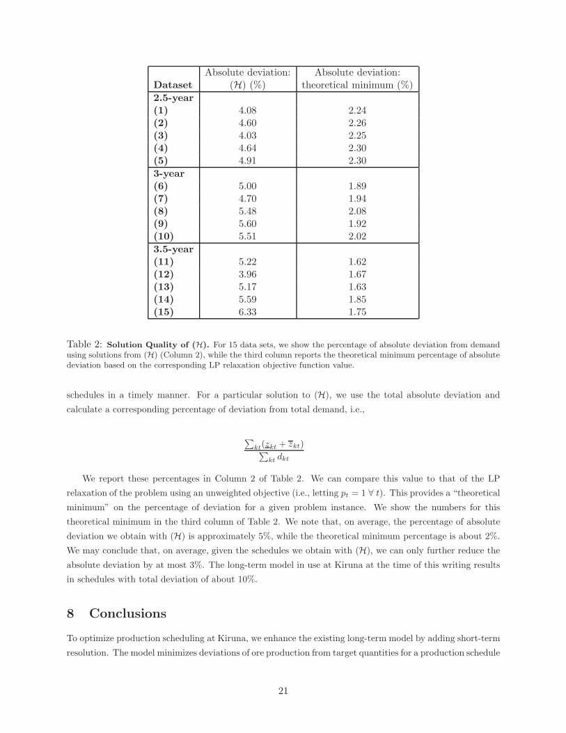
Absolute deviation: Absolute deviation:Dataset (H) (%) theoretical minimum (%)

2.5-year(1) 4.08 2.24(2) 4.60 2.26(3) 4.03 2.25(4) 4.64 2.30(5) 4.91 2.30

3-year(6) 5.00 1.89(7) 4.70 1.94(8) 5.48 2.08(9) 5.60 1.92(10) 5.51 2.02

3.5-year(11) 5.22 1.62(12) 3.96 1.67(13) 5.17 1.63(14) 5.59 1.85(15) 6.33 1.75

Table 2: Solution Quality of (H). For 15 data sets, we show the percentage of absolute deviation from demandusing solutions from (H) (Column 2), while the third column reports the theoretical minimum percentage of absolutedeviation based on the corresponding LP relaxation objective function value.

schedules in a timely manner. For a particular solution to (H), we use the total absolute deviation and

calculate a corresponding percentage of deviation from total demand, i.e.,

∑

kt(zkt + zkt)∑

kt dkt

We report these percentages in Column 2 of Table 2. We can compare this value to that of the LP

relaxation of the problem using an unweighted objective (i.e., letting pt = 1 ∀ t). This provides a “theoretical

minimum” on the percentage of deviation for a given problem instance. We show the numbers for this

theoretical minimum in the third column of Table 2. We note that, on average, the percentage of absolute

deviation we obtain with (H) is approximately 5%, while the theoretical minimum percentage is about 2%.

We may conclude that, on average, given the schedules we obtain with (H), we can only further reduce the

absolute deviation by at most 3%. The long-term model in use at Kiruna at the time of this writing results

in schedules with total deviation of about 10%.

8 Conclusions

To optimize production scheduling at Kiruna, we enhance the existing long-term model by adding short-term

resolution. The model minimizes deviations of ore production from target quantities for a production schedule

21

with monthly time periods and incorporates various operational requirements unique to sublevel caving. The

resulting model is moderately large and solution times for schedules of requisite length are excessive. To

expedite solution time, we develop a heuristic consisting of two phases: (i) solving five subproblems, and (ii)

solving a modified version of the original model based on information gained from the subproblem solutions.

Subproblem construction primarily entails modification of the objective function to capture “extreme” cases

that the original model must consider when minimizing deviations.

We compare performance of the heuristic to solving the original model directly on 15 data sets. On

average, we find that our heuristic obtains better solutions faster than solving the original problem directly.

We also note the consistency in the performance of the heuristic when compared to (P). In the (few) instances

where the default method outperforms the heuristic, the differences are minimal; however, when the heuristic

outperforms the default method, it can do so by a large margin. In general, the heuristic produces schedules

that deviate from the demand quantities by a total of only about 5% in 1000 seconds or less. Furthermore, the

heuristic appears to have a performance advantage over the default procedure when solving larger problem

instances. If we wish to solve models with a four-year or longer time horizon, modifications to (H) are

necessary, for example, tweaking the CPLEX parameter settings on various subproblem instances. However,

with few alterations to the procedure we just described, we obtain a solution with our four-year data set

provided by Kiruna using (H) that is 4% better than that obtained with (P) within a 1000 second time

limit. If we continue solving (P ) so that the objective function matches that obtained with (H), (P) requires

a total solution time in excess of 5700 seconds. A robust heuristic such as ours allows Kiruna to plan

for the short term while accounting for the longer term. For example, planners generally update yearly

schedules once a month to account for stochasticity in ore grades, inter alia. The yearly schedules are able

to consider sequencing and other operational constraints such that one monthly plan is consistent with a

subsequent one. Planners also annually create longer-term schedules of up to five years for the marketing

department and for area preparation, which generally requires several years to complete. A tool such as ours

not only integrates short- and long-term planning decisions into one model, but also enables planners to solve

instances rapidly, allowing for alternate instances to be easily explored, e.g., different mining configurations,

minor corrections to reserve and/or demand data, and a variety of realistic scenarios; long-term planners also

appreciated this rapid solution time when generating the corresponding planning models (Kuchta, Newman

and Topal (2004)). An extension to our solution procedure could consider solving the monolith starting

from the solutions we obtain using the heuristic. This might aid in finding even better solutions though

overall solution times would increase as they would then consist of both heuristic and monolith solution

times. Furthermore, we suspect that the gaps between our heuristically obtained solutions and the bounds

on these solutions is a function of a weak bound rather than a poor quality solution. Therefore, we did not

explore this strategy.

Other resource-constrained scheduling problems share an objective similar to the somewhat unconven-

tional one in this model. For example, Kirk (1999) chooses weapons on U.S. Navy ships to assign to tasks.

In his multi-objective integer program, one objective is to minimize the deviation between the weapons

remaining on a ship after the weapons have been allocated to the tasks (and fired) and the average number

of weapons remaining across all ships. Another application might be to minimize the deviation between the

preplanned (desired) and actual preventative maintenance time on equipment. Brown et al. (1997) give a

variety of examples of integer programming scheduling models whose modified solutions, in the absence of

22

persistence constraints, might exhibit large deviations from the corresponding original schedules given only

minor changes in the input data. In order to prevent such drastically different solutions from occurring, a

modified schedule might be sought subject to penalties for changes from an original solution. These changes

would generally be measured according to the (linearizable) L-1 norm, as in our problem. An approach

similar to the one we introduce here might therefore be useful in these more general settings.

Acknowledgements

We would like to thank Professor Kevin Wood of the Naval Postgraduate School for his guidance on the

algorithm format (Appendix) and helpful comments on earlier drafts of this paper. We would like to thank

Professors Alper Atamturk and Daniel Espinoza of the University of California, Berkeley and University of

Chile, respectively, for consultation and implementation help with the precedence-constrained knapsack and

conic mixed integer rounding cuts. We thank Dr. Ed Klotz of IBM for his guidance on CPLEX parameter

settings. Finally, we acknowledge the help of Kelly Eurek of the Colorado School of Mines, who retrieved

background material on sublevel caving.

23

Appendix

Additional Notation for the Early Start Algorithm

Indices, parameters and sets:

• aVa = the machine placement in AV

a that directly constrains a

• aHa = the machine placement in AH

a that directly constrains a

• ba = the number of production blocks contained in machine placement a

• s = the sublevel

• S = the set of sublevels, sorted from highest to lowest

• As = the set of machine placements on sublevel s

We use the function member(X, y) to denote the yth (greatest) member of set X .

Algorithm: Early Start Algorithm

DESCRIPTION: An algorithm to assign the earliest possible start date to a machine

placement within a sublevel caving mine.

INPUT: aVa , aH

a , ba, LHDv, As, Av ∀a ∈ A, v ∈ V, s ∈ S

OUTPUT: ES(a), the earliest possible start date for machine placement a ∀a ∈ A

{

/* Initialize the early start date values, as well as a set, Mv, containing

the LHDv greatest finish times, ordered from greatest to least. */

for(all a ∈ A) {ES(a)← 1 }

for(all v ∈ V, i = 1, ...LHDv) {member(Mv,i) ← 1 }

for(all s ∈ S) {

for(all a ∈ As) {

/* Set the early start date for a affected by the vertical sequencing constraint owing to

aVa and the corresponding number of production blocks within that machine placement.*/

ES(a)← max[ES(a), ES(aVa ) + ⌈0.5 ∗ baV

⌉]

}

/* Set the early start date according to the shaft group constraint. */

for(all v ∈ V ) {

for(all a ∈ As ∩Av) {

ES(a)← max[ES(a), member(Mv, LHDv)]

}

}

/* Set the early start date for all machine placements on the current sublevel according to

the horizontal sequencing constraints. Repeat until no changes are made. */

Set changes made = true

while(changes made = true ) {

24

Set changes made = false

for(all a ∈ As) {

/* Set the early start date for a affected by the horizontal sequencing constraints

owing to aHa . */

if(ES(aHa ) > ES(a) + ⌈0.5 ∗ ba⌉) {

ES(a)← ES(aHa )− ⌈0.5 ∗ ba⌉

Set changes made = true

}

}

}

/* Update the early start date for machine placement a and update the corresponding set

Mv ∀v such that the set contains the LHDv greatest finish times for the

machine placements for which the early start dates have been determined. */

if(ES(a) > min

a[ES(a) ∈Mv]) {

Mv ← (Mv, member(Mv, LHDv)) ∪ES(a)

}

}

}

Note that we could improve the efficiency of this algorithm (at the expense of exposition!) by executing

the while loop only until changes made has been set to true for the first time, and then resetting the affected

early start dates. The correctness of this algorithm derives from the following: machine placement a cannot

be mined any earlier than ES(a) because either the vertical and/or horizontal sequencing constraints would

be violated. To account for the resource constraint on the LHDs, we set the early start date for a machine

placement to the greater of its currently assigned early start date and the smallest early start date of the

machine placements eligible to be mined within a given shaft group. Hence, ES(a) provides a valid lower

bound on the start date for machine placement a.

25

References

Alford, C., M. Brazil and D. Lee. 2007. Optimization in underground mining. In Handbook of

Operations Research in Natural Resources. Weintraub, A. and R. Epstein, eds. Springer, 561–577.

Almgren, T. 1994. An approach to long range production and development planning with applica-

tion to the Kiruna mine, Sweden. Doctoral Dissertation 1994:143D, Lulea University of Technology,

Sweden.

AMPL Optimization LLC. 2001. AMPL, Version 10.6.16. www.ampl.com.

Atamturk, A., V. Narayanan. 2010. “Conic Mixed-Integer Rounding Cuts.” Mathematical Program-

ming 122(1) 1–20.

Boland, N., I. Dumitrescu, G. Froyland and A. Gleixner. 2007. LP-based disaggregation approaches

to solving the open pit mining production scheduling problem with block processing selectivity. Com-

puters and Operations Research. doi:10.1016/j.cor.2007.12.006.

Boyd, E.A. 1993. Polyhedral results for the precedence-constrained knapsack problem. Discrete Appl.

Math. 41(3) 185–201.

Brazil, M. and D. Thomas. 2007. Network optimization for the design of underground mines. Net-

works. 49(1) 40–50.

Brown, G., R. Dell and K. Wood. 1997. Optimization and persistence. Interfaces. 27(5) 15–37.

Caccetta, L. 2007. Application of optimisation techniques in open pit mining. In Handbook of Opera-

tions Research in Natural Resources. Weintraub, A. and R. Epstein, eds. Springer, 547–559.

Carlyle, W., B. Eaves. 2001. Underground planning at Stillwater Mining Company. Interfaces. 31(4)

50–60.

Chanda, E. 1990. An application of integer programming and simulation to production planning for

a stratiform ore body. Mining Science and Technology. 11(2) 165–172.

Dagdelen, K., M. Kuchta, E. Topal. 2002. Linear programming model applied to scheduling of iron

ore production at the Kiruna mine, Kiruna, Sweden. In Trans., Soc. for Mining, Metallurgy, and

Exploration. 312 194–198.

Danna, E., E. Rothberg, C. Le Pape. 2005. Exploring relaxation induced neighborhoods to improve

MIP solutions. Math. Programming. 102(1) 71–91.

Demeulemeester, E., W. Herroelen. 1992. A branch-and-bound procedure for the multiple resource-

constrained project scheduling problem. Mgmt. Sci. 38(12) 1803–1818.

Fourer, R., D. Gay, B. Kernighan. 2003. AMPL: A Modeling Language for Mathematical Program-

ming. Thompson Learning, Pacific Grove, CA.

26

Frimpong, S., E. Asa and J. Szymanski. 2002. Advances in open pit mine design and optimization

research. International Journal of Surface Mining, Reclamation and Environment 16(2) 134–143.

Garey, M., D. Johnson. 1979. Computers and Intractability: A Guide to the Theory of NP-Completeness.

W. H. Freeman and Company, San Francisco.

Golenko-Ginzburg, D., A. Gonik. 1997. Stochastic network project scheduling with non- consumable

limited resources. Internat. J. of Production Econom. 48 29–37.

Hochbaum, D., A. Chen. 2000. Performance analysis and best implementations of old and new

algorithms for the open-pit mining problem. Opr. Res. 48(6) 894–914.

ILOG Corporation. 2005. CPLEX, Version 9.0. www.ilog.com.

Jawed, M. 1993. Optimal production planning in underground coal mines through goal programming

– A case study from an Indian mine. In Proc., 24th Internat. Sympos. of the Appl. of Comput. in

the Mineral Indust. (APCOM). Montreal, Quebec, Canada, 43–50.

Klotz, E. Personal Communication, August 30, 2010.

Kirk, B. 1999. Tomahawk Strike Coordinator Predesignation: Optimizing Firing Platform and

Weapon Allocation. Master’s thesis, Naval Postgraduate School, Monterey, CA.

Lerchs, H., I. Grossman. 1965. Optimum design of open pit mines. In Trans., Canadian Mining Inst.

58 17–24.

Kuchta, M., A. Newman, E. Topal. 2004. Implementing a production schedule at LKAB’s Kiruna

Mine. Interfaces. 34(2) 124–134.

Minciardi, R., M. Paolucci, P. Puliafito. 1994. Development of a heuristic project scheduler under

resource constraints. Eur. J. of Oper. Res. 79(2) 176–182.

Morin, M. 2002. Underground mine design and planning: Complexity and interdependencies. Mineral

Resources Engineering 11(2) 197–215.

Newman, A., M. Kuchta. 2007. Using aggregation to optimize long-term production planning at an

underground mine. Eur. J. of Oper. Res. 176(2) 1205–1218.

Newman, A., M. Kuchta, M. Martinez. 2007. Long- and short-term production scheduling at LKAB’s

Kiruna Mine. In Handbook of Operations Research in Natural Resources. Weintraub, A. and R.

Epstein, eds. Springer.

Nudtasomboon, N., S. Randhawa. 1997. Resource-constrained project scheduling with renewable and

non-renewable resources and time-resource tradeoffs. Comput. and Indust. Engrg. 32(1) 227–242.

Osanloo, M., J. Gholamnejad and B. Karimi. 2008. Long-term open pit mine production planning:

A review of models and algorithms. International Journal of Surface Mining, Reclamation and Envi-

ronment 22 (1) 3–35.

27

Padman, R., D. Smith-Daniels, V. Smith-Daniels. 1997. Heuristic scheduling of resource- constrained

projects with cash flows. Naval Res. Logist. 44(4) 365–381.

Rahal, D., M. Smith, G. van Hout, A. von Johannides. 2003. The use of mixed integer linear

programming for long-term scheduling in block caving mines. In Proc., 31st Internat. Sympos. of the

Appl. of Comput. in the Mineral Indust. (APCOM). Capetown, South Africa, 123–131.

Rardin, R. 1998. Optimization in Operations Research. Prentice Hall, Upper Saddle River, NJ.

Sarin, S., J. West-Hansen. 2005. The long-term mine production scheduling problem. IIE Trans.

37(2) 109–121.

Smith, M., I. Sheppard, G. Karunatillake. 2003. Using MIP for strategic life-of-mine planning of the

lead/zinc stream at Mount Isa Mines. In Proc., 31st Internat. Sympos. of the Appl. of Comput. in

the Mineral Indust. (APCOM). Capetown, South Africa. 465–474.

Talbot, F. 1982. Resource-constrained project scheduling with time-resource tradeoffs: The non-

preemptive case. Mgmt. Sci. 28(10) 1197–1210.

Topal, E. 2008. Early start and late start algorithms to improve solution time for long-term under-

ground mine production scheduling. Journal of the South African Institute of Mining and Metallurgy.

108(2) 99–107.

Topal, E. 1998. Long and short term production scheduling of Kiruna iron ore mine, Kiruna, Sweden.

Master’s thesis, Colorado School of Mines, Golden, CO.

Trout, L. 1995. Underground mine production scheduling using mixed integer programming. In

Proc., 25th Internat. Sympos. of the Appl. of Comput. in the Mineral Indust. (APCOM). Brisbane,

Australia. 395–400.

Winkler, B. 1996. Using MILP to optimize period fix costs in complex mine sequencing and schedul-

ing problems. In Proc., 26th Internat. Sympos. of the Appl. of Comput. in the Mineral Indust.

(APCOM). Pennsylvania State University, PA. 441–446.

28