Embed Size (px)
Citation preview
1
A Spatial Analysis of Incomes and Institutional Quality: Evidence from US Metropolitan Areas
Jamie Bologna College of Business and Economics
West Virginia University Morgantown, WV 26505-6025
Donald J. Lacombe
Department of Agricultural and Natural Resource Economics, Department of Economics, & Regional Research Institute West Virginia University
Morgantown, WV 26506-6825 em: [email protected]
Andrew T. Young College of Business and Economics
West Virginia University Morgantown, WV 26505-6025
Keywords: institutional quality, economic freedom, income levels, income growth, spatial dependence, spillovers
JEL codes: O43, O12
This version: March 2014

2
A Spatial Analysis of Incomes and Institutional Quality: Evidence from US Metropolitan Areas
Abstract: We use the Stansel (2013) metropolitan area economic freedom index and 25 conditioning variables to analyze the spatial relationships between institutional quality and economic outcomes across 381 U.S. metropolitan areas. Specifically, we allow for spatial dependence in both the dependent and independent variables and estimate how economic freedom impacts both per-capita income growth and per-capita income levels. We find that while economic freedom and income levels are directly and positively related, increases in economic freedom in one area result in negative indirect effects on income levels in surrounding areas. In addition, we find that economic freedom has an insignificant relationship with economic growth. JEL codes: O43, O12 Keywords: institutional quality, economic freedom, income levels, income growth, spatial dependence, spillovers
3
1. Introduction
Institutional quality is widely believed to be a fundamental determinant of income levels
(Acemoglu et al. (2005) and Helpman (2008)). This belief is supported by a wealth of cross-
country empirical studies, several of which utilize the Fraser Institute’s economic freedom scores
as proxies for institutional quality.1 These scores measure the extent to which “individuals are
permitted to choose for themselves and engage in voluntary transactions as long as they do not
harm the person or property of others” (Gwartney et al., 2013, p. 1). They proxy for institutions
that are consistent with well-defined and enforced property rights, as well as for limited
government in terms of both its size and scope.
The findings of cross-country empirical studies have largely been echoed by those using
the analogous US state-level scores from the Economic Freedom of North America (EFNA)
project (Stansel and McMahon, 2013).2 Furthermore, Stansel (2013) has recently constructed US
metropolitan area-level scores based on the EFNA methodology and, using these scores, reports
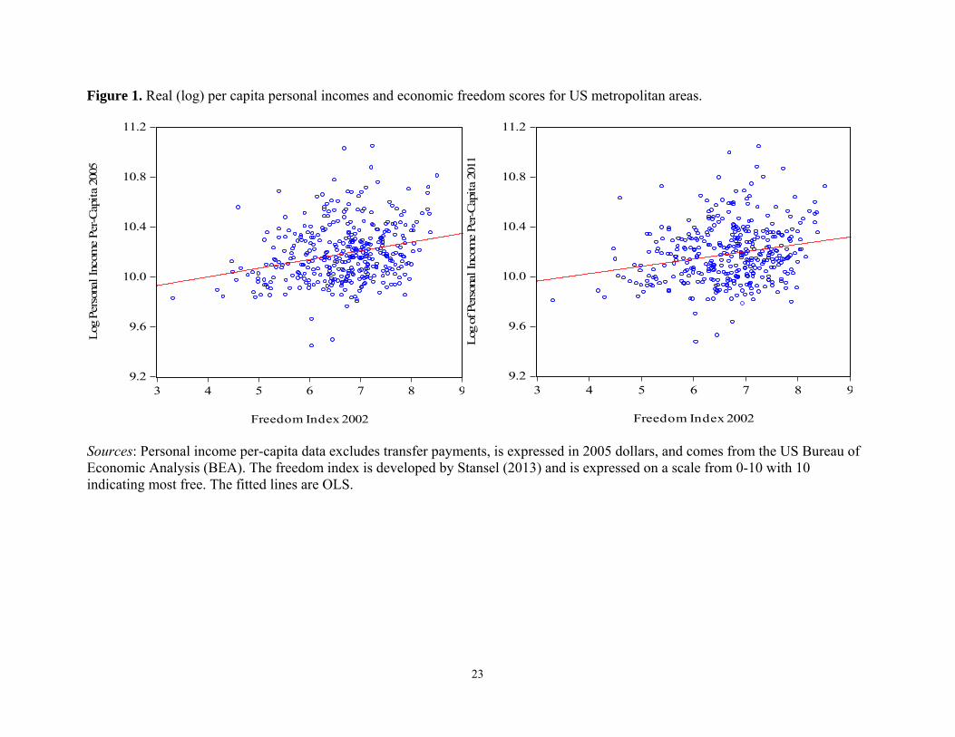
a positive income-freedom correlation.3 The positive correlation between 381 metropolitan area
(log) per capita income levels and their freedom scores is illustrated in figure 1. The left and
right panels are based on, respectively, 2005 and 2011 income levels. However, both Stansel
(2013) and figure 1 report only simple bivariate correlations. One of our goals here is to more
carefully estimate the relationship between real per capita incomes (or their growth rates) and
1 Examples of cross-country studies reporting a positive and significant relationship between economic freedom scores and per capita income levels or their rate of growth include Easton and Walker (1997), Dawson (1998), Ayal and Karras (1998), Gwartney et al. (1999), de Haan and Sturm (2000), Sturm and de Haan (2001), Lundström (2002) and Young and Sheehan (2013). For a comprehensive survey of empirical studies utilizing the Economic Freedom of the World index see Hall and Lawson (2014). 2 Karabegović et al. (2003) introduced the Economic Freedom of North America index and demonstrated that it correlated positively with income levels. (Their regressions also include observations on the 10 Canadian provinces as well as the 50 US states.) Using the US sample only, Wiseman and Young (2013) report a similar positive correlation. Kreft and Sobel (2005) and Wiseman and Young (2013) report that economic freedom is positively associated with entrepreneurial activity across US states, and Garret and Rhine (2011) find that economic freedom is associated with higher rates of employment growth. 3 Stansel (2013) specifically starts from the methodology outlined in the 2011 EFNA report (Ashby et al., 2011).

4
economic freedom in the US. We do this using Stansel’s economic freedom scores for 381
metropolitan areas along with data on personal income and 25 additional control variables.
Another of our goals is to take advantage of the large number of US metropolitan areas
and allow for spatial dependence in income levels and growth rates. Allowing for this possibility
is important and interesting for at least two reasons. First, uncontrolled-for spatial dependence
can result in inconsistent or otherwise biased estimates of the relationship between income and
economic freedom (Corrado and Fingleton, 2012). Second, there are compelling reasons to
believe that changes in one metropolitan area’s institutional quality can affect the incomes of
neighboring areas. For example, if a metropolitan area lowers its tax rates then this may increase
business activity in part by drawing customers away from businesses in neighboring areas.
Alternatively, lower tax rates can lead to increases in disposable income that are partially spent at
businesses in neighboring areas. We are interested in knowing the extent to which freedom-
increasing reforms are associated with positive sum effects; or are those effects are actually zero-
or even negative-sum once spatial dependence is taken into account?
The spatial dependence that we allow for is in geographic space. This makes sense if the
individuals, firms, and governments of geographic neighbors face lower transaction costs to
trading with and learning from one another. A geographic definition of a county’s “neighbors”
also ensures that the weight matrix employed in our estimations is independent of the variation in
our control variables; i.e., the weight is exogenous. Given our focus on geographic space, our
paper is similar to Ahmad and Hall’s (2012) study of the relationship between institutions and
income growth across 58 countries, and also to Arbia et al.’s (2010) study based on a sample of
5
271 NUTS-2 territorial units across 29 European countries.4 However, neither set of authors
calculate estimates of the direct, indirect, and total effects in the way described by LeSage and
Pace (2009). Doing so is important because, for any econometric model that includes a spatial
lag of the dependent variable, the spillover and feedback effects make the interpretation of
coefficients more complex than in the case of OLS.5 We improve upon recent practice in the
literature and report the correct direct, indirect, and total effects estimates as described by
LeSage and Pace (2009).
While the estimated direct effects of economic freedom on metropolitan area income
levels are positive, the indirect effects on neighboring areas are negative, statistically significant,
and of comparable size to the direct effects. When we examine income growth rates the evidence
is considerably weaker. We find that over 3 years the direct effect of economic freedom is
positive while the indirect effect is statistically insignificant. However, over 9 years the
estimated effects, direct or indirect, are statistically insignificant.
We organize this paper as follows. In section 2 we describe the data, with particular
attention given to Stansel’s (2013) economic freedom index. In section 3 we explain our choice
of empirical models and estimation method. We report and discuss our results in section 4. Then
we offer some summary conclusions and comments in section 5.
2. Data
4 In some of their estimations, Arbia et al. (2010) define neighbor relationships using a nonconventional weight matrix based on geographic and institutional distances. Since economic growth can be a determinant of institutional quality, spatial weights defined in terms of institutions are likely endogenous. 5 LeSage and Fischer (2009) find that the coefficients on spatially lagged explanatory variables can actually be of a different sign than the correctly estimated indirect effects. Correct calculation of the effects estimates, then, is key to a correct qualitative (as well as quantitative) interpretation of the results.
6
The control variable of interest is the Stansel (2013) economic freedom index. An index value is
available for each of the 384 US metropolitan areas for the year 2002. The index is designed to
provide a comprehensive measure of the extent to which private property is protected from
expropriation and individuals are allowed to engage in voluntary transactions.
The index is constructed on a scale from 0 to 10, with 10 indicating most free. The
comprehensive index is an average of the scores that metropolitan areas receive for 3 areas of
economic freedom separately (each also on a scale of 0 to 10). Each area of economic freedom is
itself scored based on a number of related components:
Area 1: Size of Government: (a) government consumption expenditures by government;
(b) transfers and subsidies; (c) social security payments.
Area 2: Takings and Discriminatory Taxation: (a) total tax revenue; (b) individual
income tax revenue; (c) indirect tax revenue; (d) sales taxes collected.
Area 3: Labor Market Freedom: (a) minimum wage annual income; (b) state and local
government employment; (c) union density.
Most of the components listed above are in dollar terms and are taken as a percentage of
metropolitan area personal incomes. Government employment is taken as a percentage of total
employment, as are union employees to arrive at a measure of union density.
The 384 metropolitan areas include 355 metropolitan statistical areas (MSAs) and 29
metropolitan divisions (MDs). These MSAs and MDs are defined according to the 2009 Office
of Budget and Management definitions. The 29 MDs are portions of 11 large MSAs that Stansel
breaks down so that all of the metropolitan areas are of comparable sizes. Since we are pursuing
a spatial econometric analysis, we limit ourselves to the 381 metropolitan areas of the contiguous
US states (i.e., Alaska and Hawaii areas are excluded). As can be seen in figure 2, there is
7
considerable variation in the economic freedom scores across US metropolitan areas.
Furthermore, the scores appear to be spatially correlated. Casual inspection suggests that the
spatial correlation is not entirely accounted for by intra-state similarities.
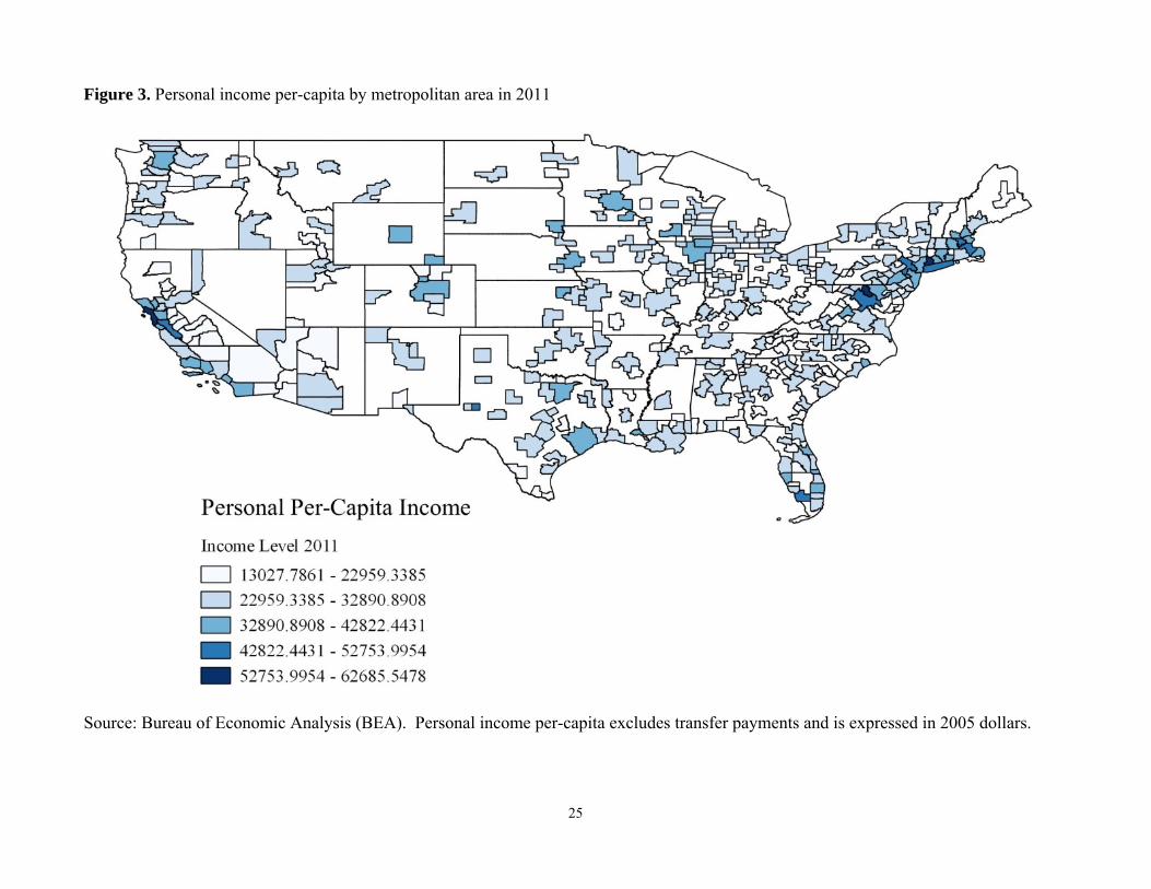
Our dependent variable will be metropolitan area real (log) personal per capita income, or
its average annual rate of growth. We use the US Bureau of Economic Analysis’s (BEA’s)
measure of personal income. The BEA’s measure of personal income includes transfer payments.
Since we are only interested in the income individuals receive from production, we will net out
the BEA’s estimate of transfer payments in each metropolitan area. Institutions and their effects
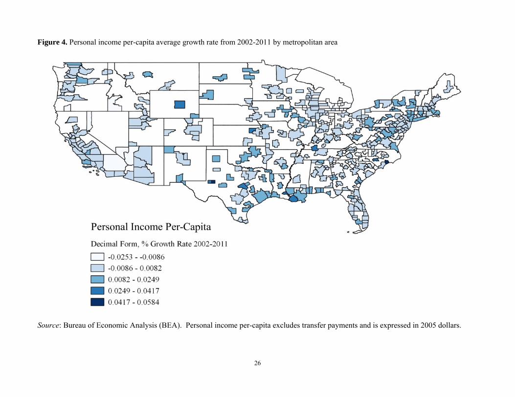
on incomes are persistent. In lieu of a well-defined time frame for those effects, we consider
income levels in 2005 and also in 2011 (or the rate of growth over 2002-2005 and also over
2002-2011.) In growth rate regressions we also include 2002 personal income per capita as an
initial income level control (to account for convergence effects). Personal income is always
converted in 2005 constant dollars.6 As in the case of economic freedom scores, per capita
income levels appear to be spatially correlated across metropolitan areas (figure 3; 2011 levels);
as do also their growth rates (figure 4; 2002-2011 growth rates).
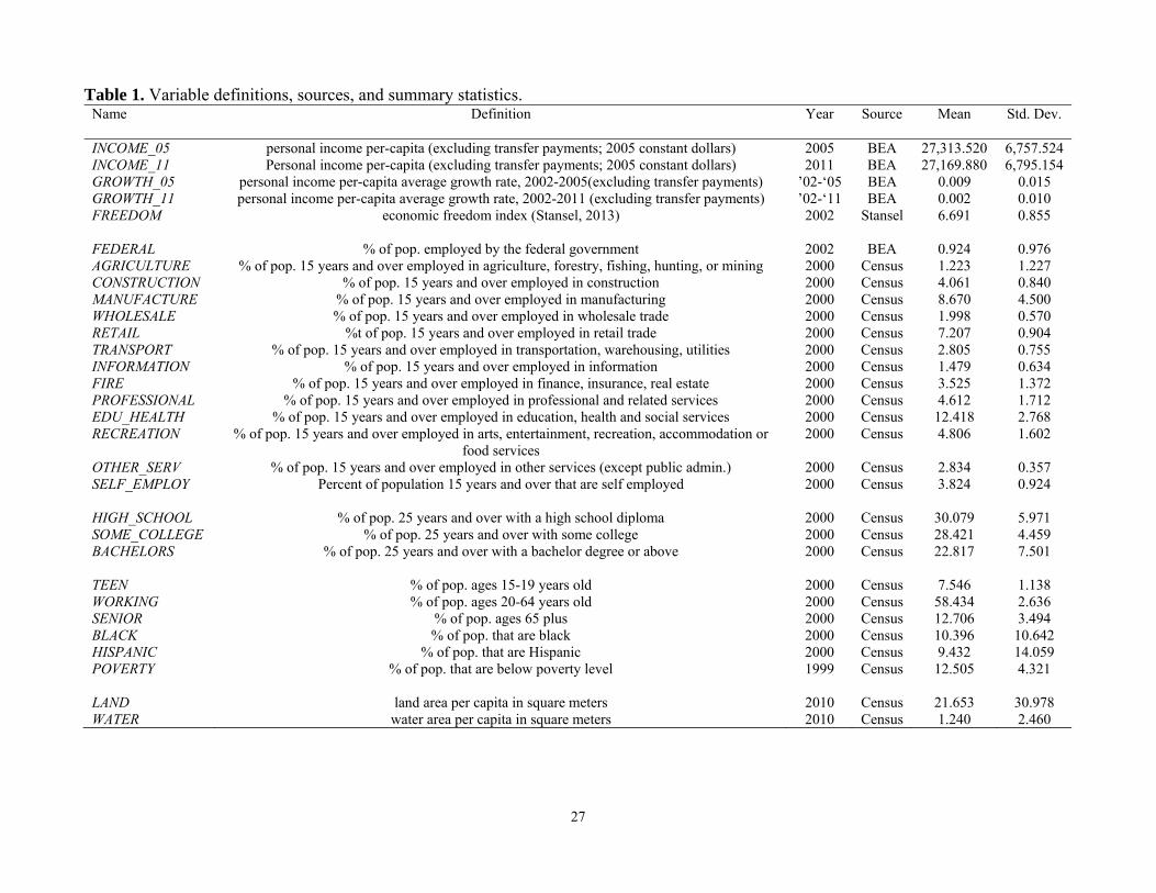
We also use 25 control variables that are motivated by Higgins et al.’s (2006) and Young
et al.’s (2010, 2013) county-level studies of income growth. These data are all from either the US
Census Bureau or the BEA.7 The control variables include (i) a number of industry employment
shares; (ii) three different educational attainment population shares (high school diploma, some
college, and bachelor’s degree or higher); and (iii) a number of demographic population shares
6 We used the World Bank’s GDP deflator. 7 All data from the BEA and the Census Bureau were extracted from February to April of 2013. The Census does not update the relevant data according to new metropolitan area definitions. Also, data from the Census is often only available at the county level. We use the 2009 metropolitan area definitions provided by the BEA to aggregate the county level components. The data from the BEA are most often available at the metropolitan level and always constructed based on the 2009 metropolitan area definitions.
8
(e.g., age and racial demographics).8 We also control for a metropolitan area’s land and water
areas per capita. All estimations include state-level fixed effects to account for unobserved
characteristics at that level.9 The data for (i), (ii), and (iii) are all based on either the year 2000 or
the year 2002.
Definitions, years, and sources for all variables are reported in table 1, along with
summary statistics.
3. Empirical Methodology and Model Choice
Our dependent variable is either a metropolitan area’s (log) real per capita income level or its
average annual growth rate. We relate this to, among other controls, a metropolitan area’s
economic freedom score from Stansel (2013). We employ Elhorst’s (2010) testing procedure to
determine whether there is spatial dependence in our data and, if there is, what is the appropriate
spatial econometric model for our analysis.
In addition to (1) OLS, the Elhorst testing procedure evaluates four spatial models: (2)
the spatial autoregressive model (SAR), (3) the spatial error model (SEM), (4) the spatial lag of
X model (SLX), and (5) the spatial Durbin model (SDM). A general form that nests each of these
alternative models is,
(3.1) WXXWyy ;
(3.2) W ,
8 Like Higgins et al. (2006) and Young et al. (2010, 2013) we control for federal government employment as a percent of a metropolitan area’s population. However, unlike those studies we do not control separately for state and local government employment. The reason for this is straightforward: state and local government employment are already a component of the freedom index’s labor market freedom area 9 For metropolitan areas that cross state borders, we follow Stansel (2013) and use the state in which the principal city of the metropolitan area resides. California is the dropped dummy variable.

9
where y is an n 1 vector of cross-sectional observations on the dependent variable; X is an n
m matrix of control variables weighted by the m 1 vector of coefficients, β; and is an n 1
vector of errors. In (3.1) and (3.2), W is an n n weight matrix that defines neighbor relations,
and are scalar parameters, and θ is a k × 1 vector of parameters (where k is the number of X
variables). defining spatial effects across neighbors. In the simplest case, if , , and are all
zero then we are left with a standard OLS model. Alternatively, spatial dependence can exist in
the dependent variable (y), the independent variables (X), or the error term (). Each of the
specific models (1) through (5) can be arrive at through parameter restrictions on the general
model (3.1) and (3.2):
OLS: = = = 0;
SAR: = = 0;
SEM: = = 0;
SLX: = = 0;
SDM: = 0.
As LeSage and Pace (2009) explain, given that the true data generating process is uncertain, in
the presence of spatial dependence the SDM model, (5), is the most likely model to produce
unbiased estimates since it is actually a generalization of models (1) through (4).10 Consequently,
SDM is likely to be the appropriate model unless testing provides statistically significant
evidence to the contrary. The Elhorst (2010) testing procedure systematically searches for such
evidence.
10 This is true because the error term is an innovation to the dependent variable and, therefore, spatial dependence in the error term amounts to spatial dependence in the dependent variable ( 0).
10
To test for spatial dependence we first need to specify the weight matrix, W. We define
neighbor relations according to a “k-nearest-neighbors” criterion. Since US metropolitan areas
have on average 6 contiguous neighboring areas, a reasonable assumption is k = 6. We therefore
define a metropolitan area’s neighbors as the 6 other metropolitan areas that are closest to the
center of its geographic mass.11 Based on the 6 closest neighbors, entries in the W matrix are
assigned 1s to indicate metropolitan area neighbor pairs. All of the other elements of W are
assigned 0s. Following convention we “row normalize” the entries such that the rows of the W
matrix all sum to one.12 While k = 6 is reasonable, it is also to some extent arbitrary. However,
for spatial models that include a parameter, as long as the estimates are interpreted properly
they will not be sensitive to this particular choice of k (LeSage and Pace, 2010).
With W specified as described above, we begin the Elhorst (2010) testing procedure by
conducting Lagrange multiplier (LM) tests to determine if there is any spatial dependence in our
data. Specifically, we estimate the OLS model and test the hypothesis of no spatial dependence
in the dependent variable (SAR) using an LM lag test; then we test the hypothesis of no spatial
dependence in the error term (SEM) using the LM error test. The appeal of these tests is that they
only require the residuals of the OLS estimation and W. A drawback of both of the LM tests is
that the specific sources of spatial dependence can sometimes be hard to distinguish from one
another (i.e., each of the standard LM tests has power over the alternative form of spatial
dependence). We employ robust versions of these LM tests that take this into account.
11 We mention above that Hawaii and Alaska metropolitan areas are not included in our sample. The reasons for this is that those metropolitan areas have such large distances from their closest neighbors that estimating the same spatial relationships as assumed for the contiguous states is unreasonable. 12When a column vector is pre-multiplied by the spatial weight matrix (e.g. Wy) the resulting vector represents an average of the neighboring observations. More importantly, row-normalization ensures that the parameter is bounded between (-1/wmin, 1/wmax) where wmin is the minimum eigenvalue of W and wmax is the maximum eigenvalue. The bounding of the parameter ensures that the variance-covariance matrix for the errors is positive definite.
11
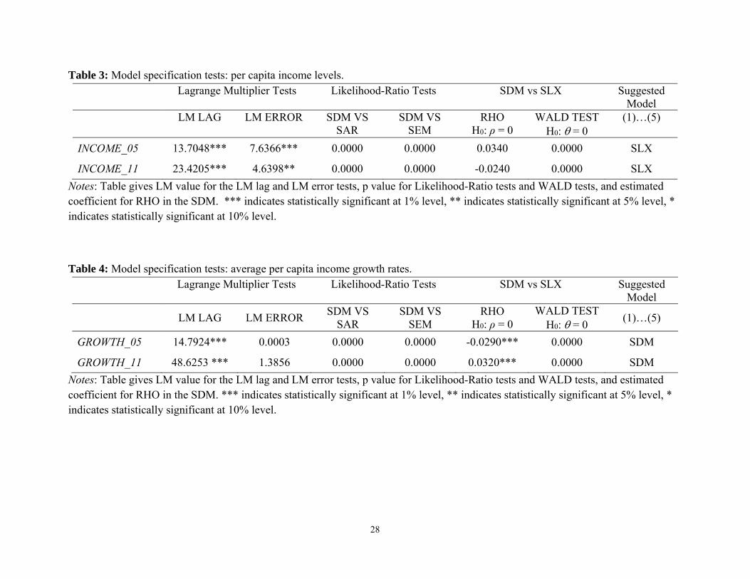
Table 3 and table 4 report the results of these LM tests for per capita income levels
(INCOME_05 and INCOME_11) and average growth rates (GROWTH_05 and GROWTH_11),
respectively. The levels are for 2005 or 2011; the average growth rates are for 2002-2005 or
2002-2011. The results are uniform. The LM tests always reject the null hypothesis of no spatial
dependence in the OLS model, suggesting that we have spatial dependence in the dependent
variable, the error term, or both.
Having rejected the null hypothesis of no spatial dependence for both income levels and
growth rates, the next step of the procedure is to estimate the SDM model to determine if the
spatial dependence is more general than either the SAR or the SEM models allow for.1 We use
the estimate of the SDM model to conduct a likelihood ratio (LR) test to determine if SDM is
more appropriate than either SAR or SEM. If SDM is found to be more appropriate than the SAR
and SEM models, we then also need to test if the parameter in the SDM model is statistically
significant once we allow for spatial dependence in the explanatory variables. Specifically, we
first test the following two hypotheses: H0: θ = 0 and H0: θ + ρβ = 0, where θ, β, and ρ are as
defined in equation (3.1). The first hypothesis is that the SDM model can be collapsed into the
SAR model, while the second hypothesis is that SDM model can be collapsed into the SEM
model. If both hypotheses are rejected, then we accept that the SDM is more appropriate than
both the SAR and SEM models. If H0: θ = 0 is not rejected then we employ the SAR model as
long as the robust LM tests point to SAR. Similarly, if H0: θ + ρβ = 0 is not rejected then we
employ the SEM model as long as the robust LM tests point to SEM. If either of these conditions
is not satisfied then the SDM model is employed by default.
Furthermore, if we deem SDM more appropriate than either SAR or SEM, or both, we
need to test if ρ is statistically different from zero in the SDM model as we are now allowing for
12
spatial dependence in the explanatory variables. If we cannot reject the null hypothesis that ρ is
statistically different from zero, we then need to re-estimate OLS including spatially lagged
explanatory variables, with no spatially lagged dependent variable, i.e. the SLX model. This
SLX estimate would be used to test the hypothesis H0: θ=0; i.e. if the spatially lagged
explanatory variables are collectively statistically different from zero. If this hypothesis cannot
be rejected, we use still use the SDM model since we found the spatial dependence in the data to
be more general than the SAR or SEM models allow.
The results from this testing procedure are reported in table 3 and table 4 for,
respectively, income levels and growth rates. Regarding income levels, the hypotheses that SDM
can be collapsed into either the SAR or SEM models are rejected in all cases. However, the
hypothesis that ρ is not statistically different from zero cannot be rejected in either case (table 3).
Also, the spatially weighted explanatory variables in the SLX model are statistically different
from zero according to a Wald test (table 3). We therefore conclude that the SLX model is the
most appropriate specification to use for the income level regressions.
For growth rates, however, the estimate of ρ is statistically different from zero in both
cases (table 4), implying that the SDM is the most appropriate model. In the case of growth
rates, then, we estimate SDM models using maximum likelihood estimation. (As opposed to the
SLX model which is estimated using OLS.) Maximum likelihood avoids the simultaneity bias in
the spatially lagged dependent variable that would have been present if we used least-squares
estimation.
4. Results

13
We begin by reporting OLS estimations (not allowing for spatial dependence) using metropolitan
area data on both (log) per capita income levels and average growth rates as the dependent
variables. To our knowledge, the present study is the first to estimate the relationship between
economic freedom and income across US metropolitan areas while controlling for a large
number of economic and demographic variables, as well as state fixed effects. The OLS results
then, both serve as useful benchmark and are interesting in their own right. We then report
estimations of spatial econometric models. Based on the Elhorst (2010) specification tests we
estimate SLX models using both the 2005 and 2011 income levels as dependent variables; and
we estimate SDM models using both the 2002-2005 and 2002-2011 annual growth rates as
dependent variables. In the growth rate estimations we include the initial (2002) (log) per capita
income level as an additional control. Otherwise the control variable set is the same across the
four spatial econometric estimations. (See section 2 above and table 1 for details on the control
variable set.)
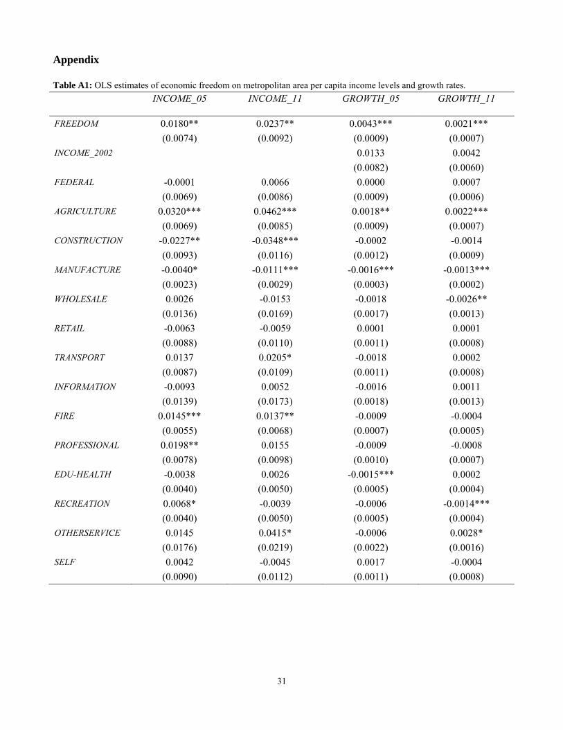
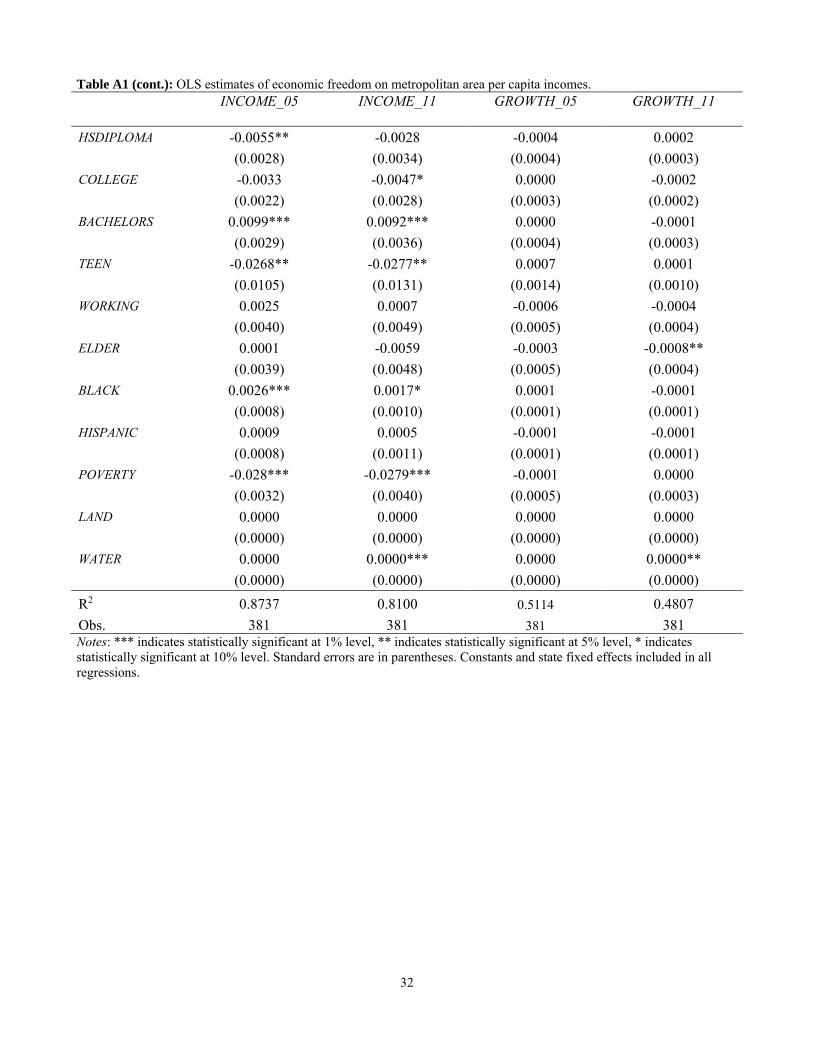
To conserve space table 5, table 6, and table 7 report only the estimated effects
associated with a metropolitan area’s 2002 economic freedom score (FREEDOM), along with
the R2 of each estimation. (In table 6 and table 7 these estimated effects include direct, indirect,
and total effects.) However, full estimation results are found in table A1, table A2, and table A3
of the appendix.
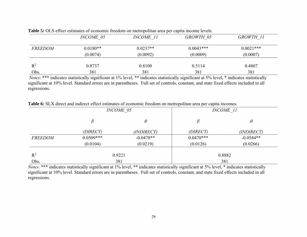
The benchmark (no spatial dependence) OLS results are reported in table 5. In all cases
we find that an increase in a metropolitan area’s 2002 freedom score is associated with a
statistically significant (5% level or better) increase in per capita income levels and growth rates.
This is consistent with the previous literature based on US state-level and cross-country level
economic freedom scores. However, the evidence reported in section 3 strongly suggests that
14
spatial dependence is present in our data. If spatial dependence is present and not controlled for
then the benchmark OLS estimates are likely to be biased. Furthermore, we are interested in
knowing not only the direct effects of a metropolitan area’s economic freedom on its income, but
also the indirect effects on its neighbors’ incomes.
Results based on the estimation of SLX income level models are reported in table 6.
Since an SLX model assumes that spatial dependence is not present in the dependent variable
(i.e., there is no ρ parameter) the estimated effects estimates can be interpreted in the same way
that one would interpret coefficients in a standard OLS regression. To identify the direct and
indirect effects, then, we need only the estimate of β and θ, respectively, from equation (3.1)
above. Based on those estimates, an increase in a metropolitan area’s 2002 freedom score is
associated with a statistically significant (1% level) increase in its own per capita income level in
2005. The same is true based on 2011 income levels and the coefficient point estimates are very
similar (0.0509 versus 0.0470). A 1 point increase in FREEDOM is associated with, all else
equal, a direct and positive effect on a metropolitan area’s per capita income level of about a 5%.
(A standard deviation increase in FREEDOM is 0.855, so its analogous direct effect on income
levels is about 4.3%.) However, the indirect effects that occur through neighbor relations are
negative and statistically significant (5% level), and the point estimates are comparable to those
of the direct effects (-0.0478 and -0.0544 for, respectively, 2005 and 2011 income levels). We
also note that the SLX models account of the largest part of the variation in the dependent
variables. (The R2s are both greater than 0.88.)
The results reported in table 6 suggest that a 1 point increase in a metropolitan area’s
economic freedom score is associated with an increase in its own per capita income of about 5%,
but also a cumulative decrease in the per capita incomes of neighboring metropolitan areas of
15
about the same size. (Importantly, an indirect effect estimate represents cumulative effects across
neighbors; not the effect per neighbor.) To put a 1 point change in the freedom score in some
perspective, the difference between the San Francisco-San-Mateo-Redwood City metropolitan
area (6.70) and the New York-White Plains-Wayne metropolitan area (4.60) is over 2 points; and
the difference between the Dallas-Plano-Irving (7.86) area and the New York-White Plains-
Wayne area is over 3 points. Despite the standard deviation of FREEDOM being less than 1
point, considerable differences in economic freedom exist across prominent metropolitan areas.
Direct and indirect effects of 5% associated with a 1 point change constitute, then, economically
large effects.
A prima facie interpretation of the table 6 results is that reforms that increase economic
freedom in a given metropolitan area lead to increases in that area’s income only at the expense
of other metropolitan areas that are not making similar reforms. As economic theory would
suggest, resources tend to relocate to metropolitan areas where taxes are lower, the security of
property rights is stronger, and regulations in labor markets are less burdensome. Over the course
of up to 9-years, our results suggest that economic activity is dampened in the areas from which
resources are relocating.
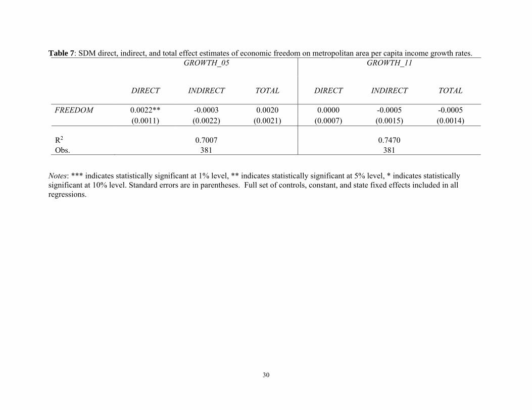
Furthermore, over the time frames that we explore, changes in FREEDOM appear to only
have significant effects on income levels. Table 7 reports the SDM model results where average
income growth rates (from 2002-2005 and 2002-2011, respectively) are the dependent variables.
Recall that since the SDM model assumes spatial dependence in the dependent variable (the ρ
parameter from (3.1)) there are feedback effects that make the interpretation of coefficient
estimates less straightforward than in the case of the SLX model. Therefore we compute correct
estimates of the direct, indirect, and total effects as described by LeSage and Pace (2009). The
16
point estimates in all cases (direct, indirect and total) are very small. Only the estimated direct
effect over the 3-year horizon is statistically significant at a conventional level (5%). The point
estimate corresponds to a 0.22 percentage change in the annual growth rate. Both indirect effect
estimates are an order of magnitude smaller and statistically insignificant. Using the 9-year
(2002-2011) average growth rate as the dependent variable, the direct effect of FREEDOM is not
only not statistically insignificant; the point estimate is also for all intents and purposes zero.
The spatial econometric results reported in table 6 and table 7 are puzzling in the sense
that they are hard to reconcile with standard economic theory. Why would a reallocation of
resources to areas providing greater economic freedom be zero-sum? A movement of resources
towards greater freedom suggests that their owners are seeking higher private returns; and to the
extent that economic freedom represents greater security of property rights, those owners will be
internalize the costs of reallocating their resources in particular ways. Higher private returns will
then, all else equal, correspond to higher social returns and the resource reallocation will be
positive-sum.
One way to reconcile the findings with theory is to assume that lower taxes and
government expenditures largely correspond to the provision of fewer productive public goods.
While higher private returns may attract businesses and customers from neighboring areas,
businesses and customers already in the reforming area may suffer offsetting losses due to less
public good provision. In this case, the change in social returns may be zero. However, why
public goods provision is not taken into account in resource reallocation decisions is unclear.
Furthermore, this story may be at odds with Higgins et al. (2009) who report that, at the US
county-level, state and local government employment are both negatively related to growth.
Another possibility is that we are not picking up the longer-run, positive sum gains from higher
17
economic freedom. We are limited in this paper to exploring relatively short time frames (at most
9-years). In the short- and even medium-run, business-stealing effects may dominate and what
appears to be a pure redistribution of resources manifests in the estimates. (By business-stealing
we refer broadly both to the stealing of an area’s customers and the actual stealing of an area’s
businesses.)
Regardless, the results reported above suggest at least two important conclusions. First, in
the short- to even medium-run metropolitan area institutional reforms may be associated gains
that are offset by comparable losses to neighboring areas. Neighboring areas may, therefore,
have an incentive to “keep up with the Jones” in terms of undertaking similar reforms.13 Second,
increases in economic freedom appear to be unrelated (or at most very weakly related) to
economic growth once spatial dependence is controlled for. The benchmark OLS growth effects
are positive and statistically significant effect (both at the 1% level; table 5). However, once
spatial dependence is controlled for these positive effects diminish or entirely disappear, at least
over the time horizons that we consider. The SDM model results reported in table 7 highlight the
importance of accounting for spatial dependence and calculating the direct, indirect, and total
effects in a way that correctly takes into account feedback.
It is important to note that the OLS point estimates bear no straightforward relationship to
either the SDM direct effects or total effects point estimates. The OLS results cannot simply be
interpreted as the correct effects conditional on neglecting spillovers. Rather, in the presence of
spatial dependence the OLS estimates are biased and inconsistent. They can only be interpreted
as non-casual (though in some ways perhaps useful) partial correlations in the data.
13 An alternative, of course, would be to somehow prevent reforms in neighboring metropolitan areas. However, how one metropolitan area can block reforms in a neighboring area is unclear. Also, if doing so is accomplished “from above” (i.e., through federal government action) then the outcome may be costly in terms of all metropolitan areas giving up a degree of autonomy.
18
5. Conclusions
A substantial empirical literature reports that economic freedom is an important determinant of
both income levels and their rates of growth. These findings seem to hold when looking both
across countries and within countries. In particular, several studies focusing on the US utilize the
state-level Economic Freedom of North America (EFNA) scores to examine this relationship.
Stansel (2013) has recently developed a US metropolitan area-level economic freedom index
based on the EFNA methodology. We utilize this new index to re-explore the relationships
between economic freedom and both income levels and growth rates.
The Stansel (2013) index allows us to contribute to the existing literature in at least two
ways. First, given the large number of metropolitan areas in the US (381 in our analysis) we are
able to carefully examine these relationships while including 25 additional control variables in
the analysis, as well as state-level fixed effects. Second, the previous literature largely ignores
the possibility of spatial dependence. Across the US, the movement of both labor and capital are
relatively cheap; it is also relatively cheap to consumers to move their purchasing activities.
Resource flows in response to institutional forms are likely to be an important part of the story.
We are interested in knowing whether freedom-increasing reforms are associated with positive
sum gains; or whether those effects are actually zero- or even negative-sum once spatial effects
are taken into account.
The results of this paper suggest at least two important conclusions: (1) the gains to
institutional reforms in a particular metropolitan area may be associated with comparable losses
to other areas that are not undertaking reforms and (2) institutional reforms seem to be unrelated
to economic growth once spatial dependence is controlled for. The conclusions can only be made
19
regarding the relatively short time horizons that we study. Since these are 3- and 9-year horizons,
(1) and (2) must be considered short- to medium-run conclusions. When more time-series data
becomes available, subsequent studies may very well find positive long-run effects associated
with increases in economic freedom. However, business-stealing effects may dominate in the
short- to medium-run that we focus on. According to our estimates, over those time horizons a 1
point increase in a metropolitan area’s economic freedom score is associated with its own per
capita income increasing by about 5% while that of its neighbors decreases (cumulatively) also
by about 5%.
20
References
Acemoglu, D., Johnson, S., Robinson, J. 2005. Institutions as a fundamental cause of economic
growth. in (Aghion and Durlauf, ed.) Handbook of Economic Growth. Amsterdam:
Elsevier.
Ahmad, M., Hall, S. G. 2012. Institutions-growth spatial dependence: an empirical test.
Procedia- Social and Behavioral Sciences 65, 925-30.
Arbia, G., Battisti, M., Di Vaio, G. 2010. Institutions and geography: empirical test of spatial
growth models for European regions. Economic Modeling 27, 12-21.
Ashby, N., Bueno, A, McMahon, F. 2011. Economic Freedom of North America 2011.
Vancouver: Fraser Institute.
Ayal, E. B., Karras, G. 1998. Components of economic freedom and growth: an empirical
study. Journal of Developing Areas 32, 327-338.
Corrado, L., Fingleton, B. 2012. Where is the economics in spatial econometrics? Journal of
Regional Science 52, 210-239.
Dawson, J. W. 1998. Institutions, investment, and growth: new cross-country and panel data
evidence. Economic Inquiry 36, 603-619.
de Haan, J., Sturm, J-E. 2000. On the relationship between economic freedom and economic
growth. European Journal of Political Economy 16, 215-241.
Elhorst, J. P. 2010. Applied spatial econometrics: raising the bar. Spatial Economic Analysis 5,
9-28.
Garrett, T. A., Rhine, R. M. 2011. Economic freedom and employment growth in U.S. states.
Federal Reserve Bank of St. Louis Review 93, 1-18.
Gwartney, J. D., Lawson, R., Holcombe, R. G. 1999. Economic freedom and the environment for

21
economic growth. Journal of Institutional and Theoretical Economics 155, 643-663.
Gwartney, J., Lawson, R. A., Hall, J. C. 2013. Economic Freedom of the World: 2013 Annual
Report. Vancouver: Fraser Institute.
Hall, J. C., Lawson, R. A. 2014. Economic Freedom of the World: An accounting of the
literature. Contemporary Economic Policy 32, 1-19.
Helpman. E. 1998. (ed.) Institutions and economic performance. Cambridge: Harvard University
Press.
Higgins, M. J., Levy, D., Young, A. T. 2006. Growth and convergence across the U.S.:
Evidence from county-level data. Review of Economics and Statistics 88, 671-681.
Higgins, M. J., Young, A. T., Levy, D. 2009. Federal, state, and local governments: evaluating
their separate roles in US growth. Public Choice 139, 493-507.
Karabegović, A., Samida, D., Schlegel, C., McMahon, F. 2003. North American economic
freedom: An index of 10 Canadian provinces and 50 US states. European Journal of
Political Economy 19, 431-452.
Kreft, S. F., Sobel, R. S. 2005. Public policy, entrepreneurship, and economic freedom. Cato
Journal 25, 595-616.
LeSage, J. P., Fischer, M. M. 2009. Spatial growth regressions: model specification, estimation
and interpretation. Spatial Economic Analysis 3, 275-304.
LeSage, J. P., Pace, R. K.2009. Introduction to Spatial Econometrics. Boca Routon: Taylor and
Francis CRC Press.
LeSage, J.P., Pace, R. K. 2010. The biggest myth in spatial econometrics. SSRN Working Paper
(http://papers.ssrn.com/sol3/papers.cfm?abstract_id=1725503).
22
Lundstrӧm, S. 2005. The effect of democracy on different categories of economic freedom.
European Journal of Political Economy 21, 967-980.
Stansel, D. 2013. An economic freedom index for U.S. metropolitan areas. Journal of Regional
Analysis & Policy 43, 3-20.
Stansel, D., McMahon, F. 2013. Economic Freedom of North America 2013. Vancouver: Fraser
Institute.
Sturm, J. E., de Haan, J. 2001. How robust is the relationship between economic freedom and
economic growth? Applied Economics 33, 839-844.
Wiseman, T., Young, A. T. 2013. Economic freedom, entrepreneurship, & income levels: some
US state-level empirics. American Journal of Entrepreneurship 6, 100-119.
Young, A. T., Higgins, M. J., Levy, D. 2010. Robust correlates of county-level growth in the
U.S. Applied Economics Letters 17, 293-296.
Young, A. T., Higgins, M. J., Levy, D. 2013. Heterogeneous convergence. Economics Letters
120, 238-241.
Young, A. T., Sheehan, K. M. 2013. Foreign aid, institutional quality, and growth. SSRN
Working Paper (http://papers.ssrn.com/sol3/papers.cfm?abstract_id=2058567).
23
Figure 1. Real (log) per capita personal incomes and economic freedom scores for US metropolitan areas.
Sources: Personal income per-capita data excludes transfer payments, is expressed in 2005 dollars, and comes from the US Bureau of Economic Analysis (BEA). The freedom index is developed by Stansel (2013) and is expressed on a scale from 0-10 with 10 indicating most free. The fitted lines are OLS.
9.2
9.6
10.0
10.4
10.8
11.2
3 4 5 6 7 8 9
Freedom Index 2002
Log
Per
sona
l In
com
e Per
-Cap
ita
2005
9.2
9.6
10.0
10.4
10.8
11.2
3 4 5 6 7 8 9
Freedom Index 2002
Log
of Per
sona
l In
com
e Per
-Cap
ita
2011

24
Figure 2. Economic freedom scores for US metropolitan areas
Source: Stansel (2013) metropolitan area economic freedom index for the year 2002. Index is on a scale of 0-10 with 10 indicating most free.
25
Figure 3. Personal income per-capita by metropolitan area in 2011
Source: Bureau of Economic Analysis (BEA). Personal income per-capita excludes transfer payments and is expressed in 2005 dollars.
26
Figure 4. Personal income per-capita average growth rate from 2002-2011 by metropolitan area
Source: Bureau of Economic Analysis (BEA). Personal income per-capita excludes transfer payments and is expressed in 2005 dollars.
27
Table 1. Variable definitions, sources, and summary statistics. Name
Definition Year Source Mean Std. Dev.
INCOME_05 personal income per-capita (excluding transfer payments; 2005 constant dollars) 2005 BEA 27,313.520 6,757.524 INCOME_11 Personal income per-capita (excluding transfer payments; 2005 constant dollars) 2011 BEA 27,169.880 6,795.154 GROWTH_05 personal income per-capita average growth rate, 2002-2005(excluding transfer payments) ’02-‘05 BEA 0.009 0.015 GROWTH_11 personal income per-capita average growth rate, 2002-2011 (excluding transfer payments) ’02-‘11 BEA 0.002 0.010 FREEDOM economic freedom index (Stansel, 2013) 2002 Stansel 6.691 0.855 FEDERAL % of pop. employed by the federal government 2002 BEA 0.924 0.976 AGRICULTURE % of pop. 15 years and over employed in agriculture, forestry, fishing, hunting, or mining 2000 Census 1.223 1.227 CONSTRUCTION % of pop. 15 years and over employed in construction 2000 Census 4.061 0.840 MANUFACTURE % of pop. 15 years and over employed in manufacturing 2000 Census 8.670 4.500 WHOLESALE % of pop. 15 years and over employed in wholesale trade 2000 Census 1.998 0.570 RETAIL %t of pop. 15 years and over employed in retail trade 2000 Census 7.207 0.904 TRANSPORT % of pop. 15 years and over employed in transportation, warehousing, utilities 2000 Census 2.805 0.755 INFORMATION % of pop. 15 years and over employed in information 2000 Census 1.479 0.634 FIRE % of pop. 15 years and over employed in finance, insurance, real estate 2000 Census 3.525 1.372 PROFESSIONAL % of pop. 15 years and over employed in professional and related services 2000 Census 4.612 1.712 EDU_HEALTH % of pop. 15 years and over employed in education, health and social services 2000 Census 12.418 2.768 RECREATION % of pop. 15 years and over employed in arts, entertainment, recreation, accommodation or
food services 2000 Census 4.806 1.602
OTHER_SERV % of pop. 15 years and over employed in other services (except public admin.) 2000 Census 2.834 0.357 SELF_EMPLOY Percent of population 15 years and over that are self employed 2000 Census 3.824 0.924 HIGH_SCHOOL % of pop. 25 years and over with a high school diploma 2000 Census 30.079 5.971 SOME_COLLEGE % of pop. 25 years and over with some college 2000 Census 28.421 4.459 BACHELORS % of pop. 25 years and over with a bachelor degree or above 2000 Census 22.817 7.501 TEEN % of pop. ages 15-19 years old 2000 Census 7.546 1.138 WORKING % of pop. ages 20-64 years old 2000 Census 58.434 2.636 SENIOR % of pop. ages 65 plus 2000 Census 12.706 3.494 BLACK % of pop. that are black 2000 Census 10.396 10.642 HISPANIC % of pop. that are Hispanic 2000 Census 9.432 14.059 POVERTY % of pop. that are below poverty level 1999 Census 12.505 4.321 LAND land area per capita in square meters 2010 Census 21.653 30.978 WATER water area per capita in square meters 2010 Census 1.240 2.460
28
Table 3: Model specification tests: per capita income levels. Lagrange Multiplier Tests Likelihood-Ratio Tests SDM vs SLX Suggested
Model LM LAG LM ERROR SDM VS
SAR SDM VS
SEM RHO
H0: ρ = 0 WALD TEST
H0: = 0
(1)…(5)
INCOME_05 13.7048*** 7.6366*** 0.0000 0.0000 0.0340 0.0000 SLX
INCOME_11 23.4205*** 4.6398** 0.0000 0.0000 -0.0240 0.0000 SLX
Notes: Table gives LM value for the LM lag and LM error tests, p value for Likelihood-Ratio tests and WALD tests, and estimated coefficient for RHO in the SDM. *** indicates statistically significant at 1% level, ** indicates statistically significant at 5% level, * indicates statistically significant at 10% level.
Table 4: Model specification tests: average per capita income growth rates.
Lagrange Multiplier Tests Likelihood-Ratio Tests SDM vs SLX Suggested Model
LM LAG LM ERROR
SDM VS SAR
SDM VS SEM
RHO H0: ρ = 0
WALD TEST H0: = 0
(1)…(5)
GROWTH_05 14.7924*** 0.0003 0.0000 0.0000 -0.0290*** 0.0000 SDM
GROWTH_11 48.6253 *** 1.3856 0.0000 0.0000 0.0320*** 0.0000 SDM
Notes: Table gives LM value for the LM lag and LM error tests, p value for Likelihood-Ratio tests and WALD tests, and estimated coefficient for RHO in the SDM. *** indicates statistically significant at 1% level, ** indicates statistically significant at 5% level, * indicates statistically significant at 10% level.
29
Table 5: OLS effect estimates of economic freedom on metropolitan area per capita income levels.
INCOME_05
INCOME_11
GROWTH_05
GROWTH_11
FREEDOM 0.0180** 0.0237** 0.0043*** 0.0021*** (0.0074) (0.0092) (0.0009) (0.0007) R2 0.8737 0.8100 0.5114 0.4807 Obs. 381 381 381 381
Notes: *** indicates statistically significant at 1% level, ** indicates statistically significant at 5% level, * indicates statistically significant at 10% level. Standard errors are in parentheses. Full set of controls, constant, and state fixed effects included in all regressions.
Table 6: SLX direct and indirect effect estimates of economic freedom on metropolitan area per capita incomes.
INCOME_05
INCOME_11
β
(DIRECT)
(INDIRECT)
β
(DIRECT)
(INDIRECT) FREEDOM 0.0509*** -0.0478** 0.0470*** -0.0544** (0.0104) (0.0219) (0.0126) (0.0266) R2 0.9221 0.8882 Obs. 381 381
Notes: *** indicates statistically significant at 1% level, ** indicates statistically significant at 5% level, * indicates statistically significant at 10% level. Standard errors are in parentheses. Full set of controls, constant, and state fixed effects included in all regressions.
30
Table 7: SDM direct, indirect, and total effect estimates of economic freedom on metropolitan area per capita income growth rates.
GROWTH_05
GROWTH_11
DIRECT
INDIRECT
TOTAL
DIRECT INDIRECT TOTAL
FREEDOM 0.0022** -0.0003 0.0020 0.0000 -0.0005 -0.0005 (0.0011) (0.0022) (0.0021) (0.0007) (0.0015) (0.0014) R2 0.7007 0.7470 Obs. 381 381
Notes: *** indicates statistically significant at 1% level, ** indicates statistically significant at 5% level, * indicates statistically significant at 10% level. Standard errors are in parentheses. Full set of controls, constant, and state fixed effects included in all regressions.
31
Appendix Table A1: OLS estimates of economic freedom on metropolitan area per capita income levels and growth rates.
INCOME_05
INCOME_11
GROWTH_05
GROWTH_11
FREEDOM 0.0180** 0.0237** 0.0043*** 0.0021***
(0.0074) (0.0092) (0.0009) (0.0007)
INCOME_2002 0.0133 0.0042
(0.0082) (0.0060)
FEDERAL -0.0001 0.0066 0.0000 0.0007
(0.0069) (0.0086) (0.0009) (0.0006)
AGRICULTURE 0.0320*** 0.0462*** 0.0018** 0.0022***
(0.0069) (0.0085) (0.0009) (0.0007)
CONSTRUCTION -0.0227** -0.0348*** -0.0002 -0.0014
(0.0093) (0.0116) (0.0012) (0.0009)
MANUFACTURE -0.0040* -0.0111*** -0.0016*** -0.0013***
(0.0023) (0.0029) (0.0003) (0.0002)
WHOLESALE 0.0026 -0.0153 -0.0018 -0.0026**
(0.0136) (0.0169) (0.0017) (0.0013)
RETAIL -0.0063 -0.0059 0.0001 0.0001
(0.0088) (0.0110) (0.0011) (0.0008)
TRANSPORT 0.0137 0.0205* -0.0018 0.0002
(0.0087) (0.0109) (0.0011) (0.0008)
INFORMATION -0.0093 0.0052 -0.0016 0.0011
(0.0139) (0.0173) (0.0018) (0.0013)
FIRE 0.0145*** 0.0137** -0.0009 -0.0004
(0.0055) (0.0068) (0.0007) (0.0005)
PROFESSIONAL 0.0198** 0.0155 -0.0009 -0.0008
(0.0078) (0.0098) (0.0010) (0.0007)
EDU-HEALTH -0.0038 0.0026 -0.0015*** 0.0002
(0.0040) (0.0050) (0.0005) (0.0004)
RECREATION 0.0068* -0.0039 -0.0006 -0.0014***
(0.0040) (0.0050) (0.0005) (0.0004)
OTHERSERVICE 0.0145 0.0415* -0.0006 0.0028*
(0.0176) (0.0219) (0.0022) (0.0016)
SELF 0.0042 -0.0045 0.0017 -0.0004
(0.0090) (0.0112) (0.0011) (0.0008)
32
Table A1 (cont.): OLS estimates of economic freedom on metropolitan area per capita incomes.
INCOME_05
INCOME_11
GROWTH_05
GROWTH_11
HSDIPLOMA -0.0055** -0.0028 -0.0004 0.0002
(0.0028) (0.0034) (0.0004) (0.0003)
COLLEGE -0.0033 -0.0047* 0.0000 -0.0002
(0.0022) (0.0028) (0.0003) (0.0002)
BACHELORS 0.0099*** 0.0092*** 0.0000 -0.0001
(0.0029) (0.0036) (0.0004) (0.0003)
TEEN -0.0268** -0.0277** 0.0007 0.0001
(0.0105) (0.0131) (0.0014) (0.0010)
WORKING 0.0025 0.0007 -0.0006 -0.0004
(0.0040) (0.0049) (0.0005) (0.0004)
ELDER 0.0001 -0.0059 -0.0003 -0.0008**
(0.0039) (0.0048) (0.0005) (0.0004)
BLACK 0.0026*** 0.0017* 0.0001 -0.0001
(0.0008) (0.0010) (0.0001) (0.0001)
HISPANIC 0.0009 0.0005 -0.0001 -0.0001
(0.0008) (0.0011) (0.0001) (0.0001)
POVERTY -0.028*** -0.0279*** -0.0001 0.0000
(0.0032) (0.0040) (0.0005) (0.0003)
LAND 0.0000 0.0000 0.0000 0.0000
(0.0000) (0.0000) (0.0000) (0.0000)
WATER 0.0000 0.0000*** 0.0000 0.0000**
(0.0000) (0.0000) (0.0000) (0.0000)
R2 0.8737 0.8100 0.5114 0.4807
Obs. 381 381 381 381 Notes: *** indicates statistically significant at 1% level, ** indicates statistically significant at 5% level, * indicates statistically significant at 10% level. Standard errors are in parentheses. Constants and state fixed effects included in all regressions.
33
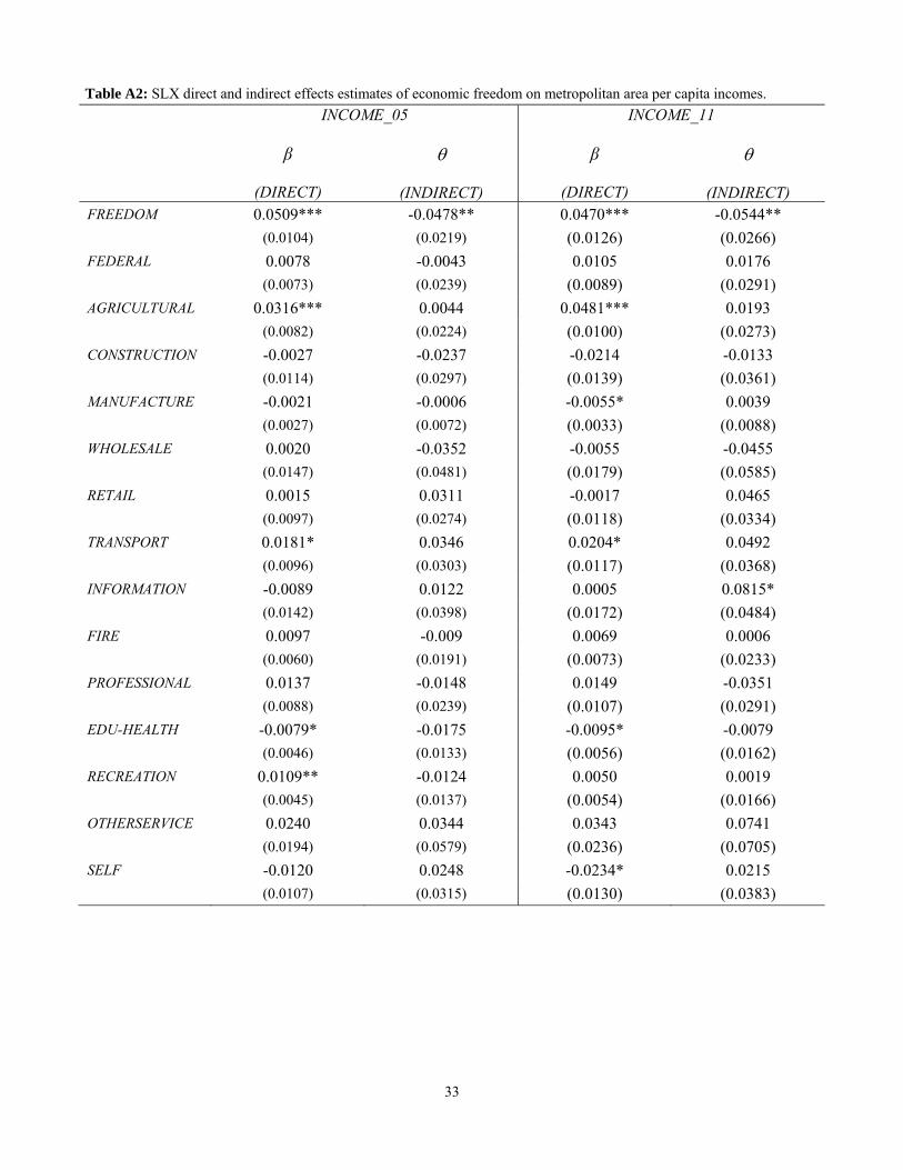
Table A2: SLX direct and indirect effects estimates of economic freedom on metropolitan area per capita incomes.
INCOME_05
INCOME_11
β
(DIRECT)
(INDIRECT)
β
(DIRECT)
(INDIRECT) FREEDOM 0.0509*** -0.0478** 0.0470*** -0.0544**
(0.0104) (0.0219) (0.0126) (0.0266)
FEDERAL 0.0078 -0.0043 0.0105 0.0176
(0.0073) (0.0239) (0.0089) (0.0291)
AGRICULTURAL 0.0316*** 0.0044 0.0481*** 0.0193
(0.0082) (0.0224) (0.0100) (0.0273)
CONSTRUCTION -0.0027 -0.0237 -0.0214 -0.0133
(0.0114) (0.0297) (0.0139) (0.0361)
MANUFACTURE -0.0021 -0.0006 -0.0055* 0.0039
(0.0027) (0.0072) (0.0033) (0.0088)
WHOLESALE 0.0020 -0.0352 -0.0055 -0.0455
(0.0147) (0.0481) (0.0179) (0.0585)
RETAIL 0.0015 0.0311 -0.0017 0.0465
(0.0097) (0.0274) (0.0118) (0.0334)
TRANSPORT 0.0181* 0.0346 0.0204* 0.0492
(0.0096) (0.0303) (0.0117) (0.0368)
INFORMATION -0.0089 0.0122 0.0005 0.0815*
(0.0142) (0.0398) (0.0172) (0.0484)
FIRE 0.0097 -0.009 0.0069 0.0006
(0.0060) (0.0191) (0.0073) (0.0233)
PROFESSIONAL 0.0137 -0.0148 0.0149 -0.0351
(0.0088) (0.0239) (0.0107) (0.0291)
EDU-HEALTH -0.0079* -0.0175 -0.0095* -0.0079
(0.0046) (0.0133) (0.0056) (0.0162)
RECREATION 0.0109** -0.0124 0.0050 0.0019
(0.0045) (0.0137) (0.0054) (0.0166)
OTHERSERVICE 0.0240 0.0344 0.0343 0.0741
(0.0194) (0.0579) (0.0236) (0.0705)
SELF -0.0120 0.0248 -0.0234* 0.0215
(0.0107) (0.0315) (0.0130) (0.0383)
34
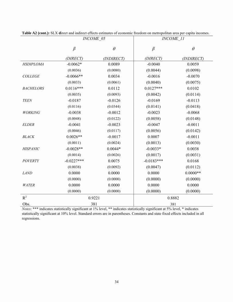
Table A2 (cont.): SLX direct and indirect effects estimates of economic freedom on metropolitan area per capita incomes.
INCOME_05
INCOME_11
β
(DIRECT)
(INDIRECT)
β
(DIRECT)
(INDIRECT) HSDIPLOMA -0.0062* 0.0089 -0.0040 0.0059
(0.0036) (0.0080) (0.0044) (0.0098)
COLLEGE -0.0066** 0.0034 -0.0016 -0.0070
(0.0033) (0.0061) (0.0040) (0.0075)
BACHELORS 0.0116*** 0.0112 0.0127*** 0.0102
(0.0035) (0.0093) (0.0042) (0.0114)
TEEN -0.0187 -0.0126 -0.0169 -0.0113
(0.0116) (0.0344) (0.0141) (0.0418)
WORKING -0.0038 -0.0012 -0.0023 -0.0068
(0.0048) (0.0122) (0.0058) (0.0148)
ELDER -0.0041 -0.0023 -0.0047 -0.0011
(0.0046) (0.0117) (0.0056) (0.0142)
BLACK 0.0026** -0.0017 0.0007 -0.0011
(0.0011) (0.0024) (0.0013) (0.0030)
HISPANIC -0.0028** 0.0044* -0.0033* 0.0038
(0.0014) (0.0026) (0.0017) (0.0031)
POVERTY -0.0227*** 0.0075 -0.0183*** 0.0168
(0.0038) (0.0092) (0.0047) (0.0112)
LAND 0.0000 0.0000 0.0000 0.0000**
(0.0000) (0.0000) (0.0000) (0.0000)
WATER 0.0000 0.0000 0.0000 0.0000
(0.0000) (0.0000) (0.0000) (0.0000)
R2 0.9221 0.8882
Obs. 381 381 Notes: *** indicates statistically significant at 1% level, ** indicates statistically significant at 5% level, * indicates statistically significant at 10% level. Standard errors are in parentheses. Constants and state fixed effects included in all regressions.
35
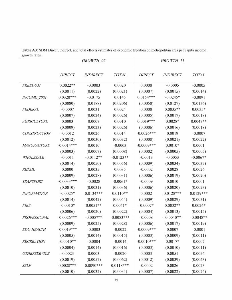
Table A3: SDM Direct, indirect, and total effects estimates of economic freedom on metropolitan area per capita income growth rates.
GROWTH_05
GROWTH_11
DIRECT
INDIRECT
TOTAL
DIRECT INDIRECT TOTAL
FREEDOM 0.0022** -0.0003 0.0020 0.0000 -0.0005 -0.0005
(0.0011) (0.0022) (0.0021) (0.0007) (0.0015) (0.0014)
INCOME_2002 0.0320*** -0.0175 0.0145 0.0154*** -0.0245* -0.0091
(0.0080) (0.0188) (0.0206) (0.0050) (0.0127) (0.0136)
FEDERAL -0.0007 0.0031 0.0024 0.0000 0.0035** 0.0035*
(0.0007) (0.0024) (0.0026) (0.0005) (0.0017) (0.0018)
AGRICULTURE 0.0003 0.0007 0.0010 0.0019*** 0.0028* 0.0047**
(0.0009) (0.0023) (0.0026) (0.0006) (0.0016) (0.0018)
CONSTRUCTION -0.0012 0.0026 0.0014 -0.0026*** 0.0019 -0.0007
(0.0012) (0.0030) (0.0032) (0.0008) (0.0021) (0.0022)
MANUFACTURE -0.0014*** 0.0010 -0.0003 -0.0009*** 0.0010* 0.0001
(0.0003) (0.0007) (0.0008) (0.0002) (0.0005) (0.0005)
WHOLESALE -0.0011 -0.0112** -0.0123** -0.0013 -0.0053 -0.0067*
(0.0014) (0.0050) (0.0056) (0.0009) (0.0034) (0.0037)
RETAIL 0.0000 0.0035 0.0035 -0.0002 0.0028 0.0026
(0.0009) (0.0028) (0.0031) (0.0006) (0.0019) (0.0020)
TRANSPORT -0.0033*** -0.0028 -0.0061* -0.0009 0.0010 0.0001
(0.0010) (0.0031) (0.0036) (0.0006) (0.0020) (0.0023)
INFORMATION -0.0025* 0.0134*** 0.0110** 0.0002 0.0128*** 0.0129***
(0.0014) (0.0042) (0.0044) (0.0009) (0.0029) (0.0031)
FIRE -0.0010* 0.0051** 0.0041* -0.0007* 0.0032** 0.0024*
(0.0006) (0.0020) (0.0022) (0.0004) (0.0013) (0.0015)
PROFESSIONAL -0.0026*** -0.0057** -0.0083*** -0.0008 -0.0040** -0.0048**
(0.0009) (0.0025) (0.0028) (0.0006) (0.0017) (0.0019)
EDU-HEALTH -0.0019*** -0.0003 -0.0022 -0.0009*** 0.0007 -0.0001
(0.0005) (0.0014) (0.0015) (0.0003) (0.0009) (0.0011)
RECREATION -0.0010** -0.0004 -0.0014 -0.0010*** 0.0017* 0.0007
(0.0004) (0.0014) (0.0016) (0.0003) (0.0010) (0.0011)
OTHERSERVICE -0.0023 0.0003 -0.0020 0.0003 0.0051 0.0054
(0.0019) (0.0057) (0.0062) (0.0012) (0.0039) (0.0043)
SELF 0.0028*** 0.0090*** 0.0118*** -0.0002 0.0026 0.0023
(0.0010) (0.0032) (0.0034) (0.0007) (0.0022) (0.0024)
36
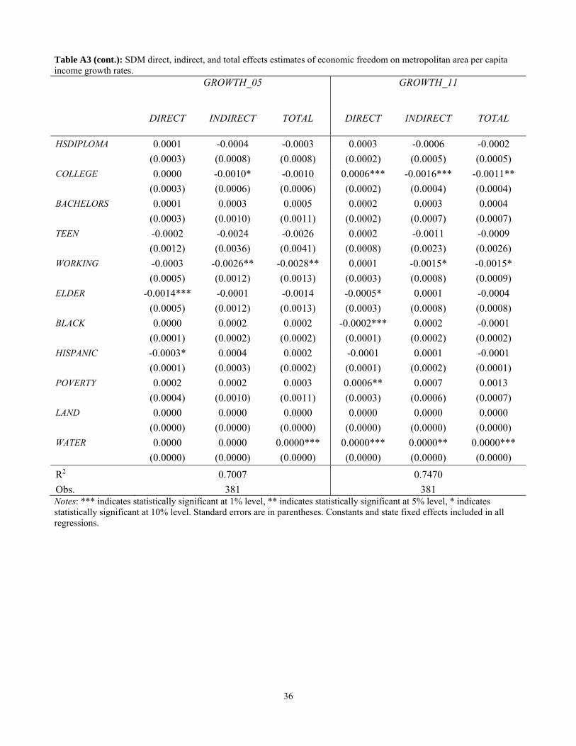
Table A3 (cont.): SDM direct, indirect, and total effects estimates of economic freedom on metropolitan area per capita income growth rates.
GROWTH_05
GROWTH_11
DIRECT
INDIRECT
TOTAL
DIRECT
INDIRECT
TOTAL
HSDIPLOMA 0.0001 -0.0004 -0.0003 0.0003 -0.0006 -0.0002
(0.0003) (0.0008) (0.0008) (0.0002) (0.0005) (0.0005)
COLLEGE 0.0000 -0.0010* -0.0010 0.0006*** -0.0016*** -0.0011**
(0.0003) (0.0006) (0.0006) (0.0002) (0.0004) (0.0004)
BACHELORS 0.0001 0.0003 0.0005 0.0002 0.0003 0.0004
(0.0003) (0.0010) (0.0011) (0.0002) (0.0007) (0.0007)
TEEN -0.0002 -0.0024 -0.0026 0.0002 -0.0011 -0.0009
(0.0012) (0.0036) (0.0041) (0.0008) (0.0023) (0.0026)
WORKING -0.0003 -0.0026** -0.0028** 0.0001 -0.0015* -0.0015*
(0.0005) (0.0012) (0.0013) (0.0003) (0.0008) (0.0009)
ELDER -0.0014*** -0.0001 -0.0014 -0.0005* 0.0001 -0.0004
(0.0005) (0.0012) (0.0013) (0.0003) (0.0008) (0.0008)
BLACK 0.0000 0.0002 0.0002 -0.0002*** 0.0002 -0.0001
(0.0001) (0.0002) (0.0002) (0.0001) (0.0002) (0.0002)
HISPANIC -0.0003* 0.0004 0.0002 -0.0001 0.0001 -0.0001
(0.0001) (0.0003) (0.0002) (0.0001) (0.0002) (0.0001)
POVERTY 0.0002 0.0002 0.0003 0.0006** 0.0007 0.0013
(0.0004) (0.0010) (0.0011) (0.0003) (0.0006) (0.0007)
LAND 0.0000 0.0000 0.0000 0.0000 0.0000 0.0000
(0.0000) (0.0000) (0.0000) (0.0000) (0.0000) (0.0000)
WATER 0.0000 0.0000 0.0000*** 0.0000*** 0.0000** 0.0000***
(0.0000) (0.0000) (0.0000) (0.0000) (0.0000) (0.0000)
R2 0.7007 0.7470
Obs. 381 381 Notes: *** indicates statistically significant at 1% level, ** indicates statistically significant at 5% level, * indicates statistically significant at 10% level. Standard errors are in parentheses. Constants and state fixed effects included in all regressions.