A ‘stack’ model of rate-independent

polycrystals

M Arul Kumar a Sivasambu Mahesh a,b P. Venkitanarayanan a

aDepartment of Mechanical Engineering, Indian Institute of Technology,

Kanpur 208016. India.

bDepartment of Aerospace Engineering, Indian Institute of Technology,

Kanpur 208016. India.

Abstract

A novel ‘stack’ model of a rate-independent polycrystal, which extends the ‘ALAMEL’

model of Van Houtte et al. (2005) is proposed. In the ‘stack’ model, stacks of

N neighboring ‘ALAMEL’ domains collectively accommodate the imposed macro-

scopic deformation while deforming such that velocity and traction continuity with

their neighbors is maintained. The flow law and consistency conditions are derived

and an efficient solution methodology based on the linear programming technique is

given. The present model is applied to study plastic deformation of an idealized two-

dimensional polycrystal under macroscopically imposed plane-strain tension and

simple shear constraints. Qualitative and quantitative variations in the predicted

macroscopic and microscopic response with N are presented. The constraint on in-

dividual ‘ALAMEL’ domains diminishes with stack size N but saturates for large

N . Computational effort associated with the present model is analyzed and found

to be well within one order of magnitude greater than that required to solve the

classical Taylor model. Furthermore, implementation of the consistency conditions

is found to reduce computation time by at least 50%.

Preprint submitted to Elsevier Science 1 November 2010

Key words: crystal plasticity, polycrystal model, flow law, consistency conditions,

linear programming

∗ Corresponding author

Email address: smahesh@iitk.ac.in (Sivasambu Mahesh).

2

1 Introduction

In numerical simulations of polycrystal plastic deformation (Mathur and Daw-

son, 1989, Beaudoin et al., 1993, 1995, Mika and Dawson, 1998, Barbe et al.,

2001, Ganapathysubramanian and Zabaras, 2005, Loge and Chastel, 2006,

Van Houtte et al., 2006, Guan et al., 2006, Haddadi et al., 2006, Amirkhizi

and Nemat-Nasser, 2007, Barton et al., 2008), microstructure-based predic-

tion of material point response offer advantages over phenomenology-based

predictions (Kim et al., 2008, Wang et al., 2008, Van Houtte et al., 2009, and

references therein), albeit at greater computational cost. One advantage is

that microstructure-based methods are applicable without restrictions for all

loading histories, and also typically over a wider range of strain-rates and tem-

peratures than phenomenological methods. Also, microstructure-based models

predict material response at both macro- and micro-scales. They are therefore

amenable to experimental verification at both scales (Peeters et al., 2001b,a,

Mahesh et al., 2004).

Microstructure-based polycrystal plasticity models evolve the lattice orienta-

tion and anisotropic hardening of grains in response to macroscopically im-

posed constraints on the material point. A number of microstructure-based

models are presently available. These range from the simple, yet qualita-

tively successful Taylor model (Taylor, 1938, Hirsch and Lucke, 1988a,b) to

the crystal plasticity finite element method (Kalidindi et al., 1992, Kalidindi

and Duvvuru, 2005, Kalidindi et al., 2006, Knezevic et al., 2008). While the

former assumes that each grain of the polycrystal deforms according to the

macroscopic constraint (Taylor hypothesis), the latter resolves spatial varia-

tions of deformation down to the sub-granular scale. The greater resolution

3

comes at a cost: Computationally, the former is typically two to three or-

ders of magnitude less expensive than the latter. Since most of the computa-

tional expense of numerical simulations of macroscopic processes implementing

microstructure-based material models is incurred during microstructure-level

computations (Barton et al., 2008), and since the Taylor model is compu-

tationally the lightest model available, it has been the method of choice for

microstructure-based material response prediction in macroscopic numerical

simulations (e.g., Mathur and Dawson (1989), Beaudoin et al. (1993)).

However, it is now recognized that a quantitatively imprecise model for the

evolution of the microstructure can be more deleterious to the accuracy of the

macroscopic predictions than a phenomenological model, or a model of the mi-

crostructure that does not evolve with deformation (Van Houtte et al., 2005).

The Taylor model, although qualitatively successful in predicting texture evo-

lution has several shortcomings such as its tendency to overestimate texturing

rate, its inability to predict the formation of certain experimentally observed

texture components, its unsuitability in sub-structural studies, its inability

to model intragranular phenomena, and its inapplicability to low symmetry

materials (Leffers, 1975, Leffers and Christoffersen, 1997, Leffers, 1978, Hirsch

and Lucke, 1988a,b, Christoffersen and Leffers, 1997, Mika and Dawson, 1998).

Much recent effort has therefore focused on developing modifications of the

Taylor model that, on the one hand, preserve its computational lightness,

and on the other hand, render its microstructural predictions quantitatively

accurate.

Successful approaches to modifying the Taylor model invariably hinge upon

better approximations of the stress in a grain (Leffers, 1978, Aernoudt et al.,

1993). In perhaps the earliest such approach Honneff and Mecking (1978) re-

4

laxed rolling direction shear constraints in rolling simulations by setting the

corresponding shear tractions to zero. They found that this reduced the rate of

texturing and led to better comparison between the predicted and experimen-

tal textures. The mixed deformation-rate and traction boundary condition of

Honneff and Mecking (1978), developed further by Kocks and Canova (1981),

Kocks and Chandra (1982), Van Houtte (1982), Christoffersen and Leffers

(1997) is known as relaxed constraints. It differs from full constraints wherein

all components of the deformation-rate are imposed upon a grain. Relaxed

and full constraints are ideally suited when the granular morphology is pan-

cake shaped and equiaxed, respectively. Tome et al. (1984) have provided a

technique to effect a transition from full to relaxed constraints with increasing

grain aspect ratio.

Although constraint relaxation reduces the texturing rate during plane strain

deformation, it too fails to quantitatively match the experimental texture evo-

lution (Van Houtte et al., 1999). This failure is ascribed to the neglect of

inter-granular interactions in Taylor-like models. As a first-order correction,

pairwise interaction between neighboring grains has been incorporated into

the polycrystal model. This interaction takes the form of velocity and trac-

tion continuity between neighboring grains. Depending on whether individual

grains are taken to deform homogeneously or otherwise, the continuity con-

ditions vary between two limiting forms. If inhomogeneous deformation of

grains is permitted, geometrically necessary dislocations, proposed by Ashby

(1970) will be generated within individual grains and accommodate any misfits

between the grains. If the energy stored in the geometrically necessary dislo-

cations is taken to be negligible, arbitrary misfits could be accommodated

by them. This corresponds to the case of Leffers (1975), wherein only trac-

5

tion continuity between interacting grains is enforced. This limit will be called

the S -type continuity condition below. The other limit, called the E -type

continuity condition results when the energy penalty associated with the geo-

metrically necessary dislocations accommodating misfits between neighboring

grains is very large. In this case, each grain must deform homogeneously and

compatibly with the other; the only role of geometrically necessary disloca-

tions, confined to the grain boundary, is to rotate the grains such that voids or

interpenetrations are avoided at the grain boundary (Ashby, 1970). Traction

continuity between the grains must also be preserved.

The E -type condition, which enforces velocity and traction continuity across

a grain boundary, has been employed extensively to model pairwise intergran-

ular interactions. Thus, within the self-consistent framework of Molinari et al.

(1987) and Lebensohn and Tome (1993), interaction equations for a grain with

the surrounding homogeneous effective medium were developed by Lebensohn

et al. (1998a) and Lebensohn (1999) for a grain comprised of codeforming ma-

trix and twin regions. The models of Lee et al. (2002) and Van Houtte et al.

(1999, 2005) disregard the self-consistent hypothesis and treat the polycrys-

tal as a collection of bicrystals. Each bicrystal in these models satisfies the

Taylor hypothesis, i.e., accommodates the imposed macroscopic constraints

by codeformation of its two constituent grains.

The models described above have been extended to include more than pairwise

interactions between grains. The self-consistent interaction equation derived

by Garmestani et al. (2001) extends the model of Lebensohn et al. (1998b)

and Lebensohn (1999). It considers inter-granular interaction through two-

or three-point correlation functions of lattice orientations. Similarly, the rate-

dependent and rate-independent binary-tree based models of Mahesh (2009,

6

2010) extend the models of Lee et al. (2002) and Van Houtte et al. (1999,

2005) to multi-grain interactions.

a

a

b

b

c

c

d

d

e

e fA

A

B

B

C

C

L1

L2

L3

MatrixM

atrix

Twin

(a) (b)

(c)

100 µm

100 µm

Fig. 1. Development of the ‘stack’ model from a 2-D microstructure (Manonukul

and Dunne, 2004). (a) Microstructure showing the three largest stacks, L1, L2 and

L3; (b) Discretization of grains A, B and C into ‘ALAMEL’ domains a, . . . , f ;

(c) Discretization of a grain containing an annealing twin into a stack of domains.

The ‘lamel’ (Van Houtte et al., 1999) and ‘ALAMEL’ models (Van Houtte

et al., 2005), form the starting points of the present work. In the ‘lamel’

model (Van Houtte et al., 1999), the polycrystal is regarded as a collection of

bicrystals. Each bicrystal is formed by pairing interacting neighboring grains in

the microstructure. Individual grains are assumed to deform homogeneously.

In the ‘ALAMEL’ model, grains do not deform homogeneously. Grains are

divided into domains, with one domain abutting each grain boundary facet.

Conversely, each grain-boundary facet is associated with two domains meeting

7

at that facet. It is the domains that are taken to deform homogeneously in

the ‘ALAMEL’ model. The polycrystal is regarded as a collection of bicrystals

formed by pairs of domains meeting at a grain-boundary facet. Thus, whereas

in the ‘lamel’ model, homogeneity of grain deformation is accorded greater

importance, in the ‘ALAMEL’ model, coupling between domains across a grain

boundary is taken to dominate the coupling between multiple domains within

the same grain.

The distinctions between the two models are illustrated in connection with

the experimental microstructure of Manonukul and Dunne (2004) shown in

Fig. 1. The explanation to follow centers around grains A, B and C marked

in Fig. 1a. Fig. 1b shows an enlarged view of these grains and also shows their

division into ‘ALAMEL’ domains, a . . . , f . Here, thick and thin lines denote

grain boundary facets and domain boundaries, respectively. Deformations of

grains A and B are coupled in the ‘lamel’ model, whereas, in the ‘ALAMEL’

model, it is the deformation of domain b in grain A and domain c in grain

B that are coupled with each other. On the other hand, the deformation of

domain d of grain B is coupled to that of domain e of grain C. Deformation

of domain d is unaffected by the deformation of any domain in grain A in the

‘ALAMEL’ model.

Van Houtte et al. (2004, 2005) and Van Houtte et al. (2006) have reported ex-

cellent agreement of the texture predicted by the ‘ALAMEL’ model with that

predicted by the full-field crystal plasticity finite element method provided the

division of grains into domains is judiciously done. However, no validation of

the mechanical anisotropy predictions of the ‘ALAMEL’ model is presently

available.

8

The ‘ALAMEL’ model, while being superior to both the Taylor and ‘lamel’

models, also has some deficiencies. First, each ‘ALAMEL’ pair of domains is

constrained to undergo the macroscopically imposed deformation. Thus, al-

though ‘ALAMEL’ domains are less constrained than Taylor or ‘lamel’ grains,

they are over-constrained compared to those in the self-consistent model (Leben-

sohn and Tome, 1993), grain interaction model (Engler et al., 2005), or the

binary tree based model (Mahesh, 2010). Kanjarla et al. (2010) have recently

noted significant deviation from the constraint assumed on ‘ALAMEL’ pairs

from crystal plasticity finite element simulations of an ensemble of four grains.

Second, the ‘ALAMEL’ model completely disregards intra-grain interactions.

Such interactions assume added significance in the presence of sub-struc-

tural features such as deformation twins, annealing twins (Proust et al., 2007,

Bystrzycki et al., 1997), deformation bands or shear bands (Barrett and Lev-

enson, 1940, Liu and Hansen, 1998, Paul et al., 2009). The slip activity within

such banded grains is determined by the intra-grain interaction of the banded

region with the matrix. Third, the ‘ALAMEL’ model assumes that pairwise in-

teraction between neighboring domains in the microstructure dominates other,

possibly longer range interactions, such as that between a domain and another

of its nearest neighbors or one of its next nearest neighbors. Consequences of

disregarding these other interactions are not presently quantified.

These shortcomings can be overcome in a straightforward manner by extend-

ing the ‘ALAMEL’ model to account for stacks of an arbitrary number N

of codeforming domains. The interface between any two neighboring domains

in the stack is assumed planar and oriented identically throughout the stack.

Van Houtte et al. (2005) have given an algorithm to discretize grains in a

micrograph into domains and ‘ALAMEL’ units. A systematic procedure to

9

form stacks of domains involves sequentially gluing neighboring ‘ALAMEL’

units together. Two neighboring ‘ALAMEL’ units can be glued together pro-

vided (i) one of the domains of each of the ‘ALAMEL’ units belong to the

same grain and (ii) the grain boundaries contained in the two ‘ALAMEL’

units have similar orientations (i.e., their relative inclinations fall within a

prescribed threshold). This procedure will result in the deterministic sub-di-

vision of the original micrograph into ‘stacks’ of different sizes such that every

material point in the micrograph will appear in one of the stacks. Statistical

correpondence between the original micrograph and the stack representation

is therefore automatic, not only for texture but also for the orientation of the

grain boundary facets.

The three largest ‘stacks’ (by area) obtained according to the foregoing con-

ditions from the micrograph are shown in Fig. 1a. Intra-grain boundaries are

absent in this micrograph. Fig. 1c schematically illustrates the sub-division

of a grain in the presence of an intra-granular boundary such as an annealing

twin. The twin is represented as domain c, while the matrix regions surround-

ing the twin are represented by domains b and d. These domains may also be

connected with domains of their neighboring grains, such as a and e to form

a stack. The ‘stack’ model can thus both reduce the constraint on individual

domains and account for intra-granular boundaries.

The ‘stack’ model of a polycrystal resembles the binary tree based model (Ma-

hesh, 2009, 2010) in that interaction between neighboring domains is the cen-

tral consideration of both models. In this respect, they differ from the self-

consistent models (Molinari et al., 1987, Lebensohn and Tome, 1993) where

the key interaction considered is that between a grain and the homogeneous

effective medium representing the entire polycrystal. However, whereas the

10

‘stack’ model accounts for serial interaction between many domains, the binary

tree based model treats interactions between pairs of domain sub-aggregates.

The ‘stack’ model is thus a better physical representation for microstructures

wherein banding within grains, as shown in Fig. 1c, is prominent.

In the present work, we develop the ‘stack’ model of a polycrystal. In Sec. 2 we

develop the flow law and consistency conditions for the general ‘stack’ model

and in Sec. 3 we provide an efficient algorithm for its solution in the case of

an idealized two dimensional polycrystal. Sec. 4 returns to the aforementioned

questions regarding interactions between multiple domains and its effect on

the predicted macroscopic response.

2 The ‘stack’ model

After recapitulating the standard rate-independent crystal plasticity frame-

work (Havner, 1992, Kocks et al., 1998, Asaro and Lubarda, 2006) in Sec. 2.1

below, we develop continuity condition, flow law and consistency equations for

the present ‘stack’ model in Sec. 2.2.

2.1 Plastic deformation of a domain

2.1.1 Standard rate-independent crystal plasticity

Throughout, we assume that domains deform homogeneously following a rigid-

plastic rate-independent volume preserving constitutive law. Denoting the

11

strain-rate of domain g by ǫ[g], we take

ǫ[g] =S∑

s=1

γ[g]s m

[g]s , (1)

following the Taylor-Bishop-Hill formulation (Taylor, 1938, Bishop and Hill,

1951). γ[g]s in Eq. (1) denotes the slip-rate of slip system s ∈ 1, 2, . . . , S and

m[g]s denotes the Schmid tensor of slip system s

m[g]s = (b[g]s ⊗ n[g]

s + n[g]s ⊗ b[g]s )/2, (2)

where b[g]s is the Burger’s vector or unit slip directional vector of slip system

s with slip plane normal n[g]s .

Let T [g] be the Cauchy stress in domain g and let its deviatoric part be σ[g].

Thus,

σ[g] = T [g] − p[g]I, (3)

where, p[g] = tr(T [g])/3 is the hydrostatic pressure in domain g.

Anticipating that standard linear programming will be used to solve the crystal

plasticity model, we take γ[g]s ≥ 0, for all s. Schmid’s law (Kocks et al., 1998)

states that slip system s may have non-zero slip-rate only if the resolved shear

stress, σ[g] :m[g]s ≡ tr(σ[g]m[g]

s

T), equals the critical resolved shear stress on

slip system s, τ [g]s . Thus,

γ[g]s

≥ 0, if σ[g] :m[g]s = τ [g]s ,

= 0, if σ[g] :m[g]s < τ [g]s .

(4)

Condition (4) implies that the yield surface of the rate-independent single

crystal is made of S smooth surfaces f [g]s given by

12

f [g]s = τ [g]s − σ[g] :m[g]

s = 0, s ∈ 1, 2, ..S. (5)

f [g]s is independent of p[g], i.e., the plastic response of the single crystal is

assumed to be pressure-insensitive. Slip system s∗ is said to be critical if f[g]s∗ =

0. Clearly, according to Eq. (4), non-critical slip systems must necessarily have

zero slip-rates.

Chin and Mammel (1969) have shown that Taylor’s principle (Taylor, 1938),

which asserts that for given ǫ[g] of all possible slip-rate combinations γ[g]s , s ∈

1, . . . , S that respect the constraint given by Eq. (1), those which minimize

the plastic power of deformation

W [g]p =

S∑

s=1

τ [g]s γ[g]s (6)

automatically satisfy Eq. (4). For the optimal set of slip-rates, Chin and Mam-

mel (1969) further established the equivalence of the Taylor (Taylor, 1938) and

Bishop-Hill (Bishop and Hill, 1951) formulations and established the equiva-

lence of the internal and external plastic powers, i.e.,∑

s τ[g]s γ[g]

s = σ[g] : ǫ[g].

Van Houtte and Aernoudt (1975a,b) have given a computational procedure

for the analysis of a polycrystal model by reducing Eqs. (6) and (1) to the

form of a standard linear program.

2.1.2 Kinematics

The deformation gradient F [g] of a rigid-plastic domain can be decomposed (Lee,

1969) as F [g] = R[g]latF

[g]p , where R

[g]lat denotes an orthonormal tensor signifying

lattice rotation, and F [g]p is the part of the deformation gradient accommo-

dated through slip-rate. The evolution of the deformation gradient is given by

13

(e.g., Gurtin (1981))

F [g] = L[g]F [g], (7)

where L[g] denotes the velocity gradient of the domain. Rice (1971) related

the evolution of F [g]p to slip-rate through the flow rule

F [g]p = L[g]

p F[g]p , (8)

where,

L[g]p =

S∑

s=1

γ[g]s (R

[g]lat

Tb[g]s )⊗ (R

[g]lat

Tn[g]

s ) = R[g]lat

T[

S∑

s=1

γ[g]s b

[g]s ⊗ n[g]

s

]

R[g]lat. (9)

R[g]lat

Tb[g]s andR

[g]lat

Tns are the slip direction, and slip plane normal, respectively,

of the s-th slip system in the reference configuration corresponding to F [g] =

F [g]p = I. The term within square brackets in the last step of Eq. (9) is

based on the orientation of the slip systems in the current (lattice rotated)

configuration, and will occur more frequently in what follows. It is called the

slip-rate tensor (Fleck et al., 2003), and is denoted

L[g]ss =

S∑

s=1

γ[g]s b

[g]s ⊗ n[g]

s . (10)

It is clear that L[g]p = R

[g]lat

TL[g]

ssR[g]lat. The symmetric part of the slip rate tensor,

L[g]ss , is the strain-rate of the domain, ǫ[g] = (L[g]

ss +L[g]ss

T)/2, given by Eq. (1).

The lattice rotation tensor R[g]lat of a domain evolves as

R[g]lat = Ω

[g]latR

[g]lat, (11)

where, Ω[g]lat is skew-symmetric and is called the lattice spin tensor. The velocity

gradient of the domain is comprised of contributions from slip rate, and lattice

spin as

L[g] = L[g]ss +Ω

[g]lat. (12)

14

Taken together with Eqs. (8), (9), (10) and (11), Eq. (12) implies (Pierce et al.,

1983)

L[g] = F [g]F [g]−1= R

[g]latF

[g]p F

[g]p

−1R

[g]lat

T+ R

[g]latR

[g]lat

T. (13)

2.1.3 Hardening

Sub-structural processes that accompany accumulating slip-rate typically af-

fect the state of the domain (Cuitino and Ortiz, 1992). The state evolution is

represented as the evolution of the critical resolved shear stress (τ [g]s ) following

the standard form (Hill, 1966, Kocks et al., 1998)

τ [g]s =dτ [g]

dΓ[g]

S∑

s′=1

Hss′ γ[g]s′ , (14)

where [H ] is the latent hardening matrix and Γ[g] =∑S

s=1 γ[g]s , is the total

accumulated slip in domain g. In the present work, for simplicity, we take τ [g]

to have a power law dependence on Γ[g], i.e.,

τ [g](Γ[g]) = τ0 + θ1(Γ0 + Γ[g])p, (15)

where p is called the hardening index, τ0, a scalar parameter, denotes the

initial critical resolved shear stress and θ1 is the hardening rate.

2.2 Plastic deformation of a ‘stack’

2.2.1 Geometry and notation

A stack of N domains, the central object of study in the present work, is

shown in Fig. 2a. Parallelepiped-shaped domains, g ∈ 1, 2, . . . , N, equal

in all dimensions, except possibly the thickness t[g], are stacked as shown in

15

Fig. 2a. The volume of fraction, ρ[g], of domain g is then

ρ[g] =t[g]

∑Nl=1 t

[l]. (16)

We assume that the stacking is repeated periodically ad infinitum so that

neighbors of domain g in the stack are g + 1 mod N and g − 1 mod N . In

particular, the two neighbors of domain 1 in the stack are domain N and

domain 2 and those of domain N are domain N − 1 and domain 1. In the

case that N = 2 the geometry of the ‘stack’ model reduces to that of the

twinning models of Lebensohn et al. (1998a), Lebensohn (1999) and the ‘lamel’

or ‘ALAMEL’ models of Van Houtte et al. (1999, 2002, 2005).

Domain boundaries between adjacent domains are taken to be planar and

identically orientated with the normal vector ν, as shown in Fig. 2a. Two

sets of cartesian coordinates: the sample coordinate system xyz and a domain

boundary coordinate system XY Z with its Y -axis always aligned with the

normal vector ν are also defined.

Since domains g and domain boundaries i play an important role in the follow-

ing considerations, we adopt the following conventions. Quantities associated

with domains are indicated by superscripts surrounded by square brackets,

e.g., t[g] for the thickness of domain g in Eq. (16), while quantities associated

with interfaces are indicated by superscripts surrounded by parantheses, e.g.,

λ(i) denoting the Hadamard characteristic segment of domain boundary i in

Eq. (28) below. Secondly, domains above and below, the domain boundary i

will be denoted as [a(i)] and [b(i)], respectively, while the domain-boundaries

surrounding interface i will be called (a(i)) and (b(i)), respectively, as shown

in Fig. 2b. Note that use of the terms ‘above’ and ‘below’ are for mnemonical

purposes only; their consistent interchange will not affect any other aspect of

16

the present model.

X

Y

Z

x

y

z

Limp

Limp

i = 1

i = 2

i = N

i = N

.

g=1g=2

g=N

g=N−1

t[1]

t[2]

t[N−1]

t[N ]

.

.

.

.

.

.

.

..

.

.

.

.

.

(a) (b)

ν

(i)

(a(i))

(b(i))

[b(i)]

[a(i)]

Fig. 2. (a) The ‘stack’ model comprised of N domains. (b) Nomenclature for domain

and domain boundaries.

2.2.2 Kinematics of ‘stack’

We may now extend the kinematic notions defined for a domain in Sec. 2.1.2

to a ‘stack’. The velocity gradient of a ‘stack’ is taken as the volume fraction

weighted average of that of its constituent domains, i.e.,

L =N∑

g=1

ρ[g]L[g]. (17)

If F denotes the deformation gradient of the ‘stack’, in analogy with Eq. (7)

for single domains, we define

˙F = LF . (18)

The domain boundary normal ν, defined in Sec. 2.2.1 is assumed to evolve

17

with the shape of the ‘stack’, as given by F . Thus, if ν0 is the normal vector

when F = I, according to Nanson’s formula (Gurtin, 1981),

ν =F−Tν0

‖F−Tν0‖. (19)

Time differentiating Eq. (19) and simplification using Eq. (18) gives

ν = (ν ⊗ LTν − LT )ν. (20)

2.2.3 Constraints

In the present work, we assume the full constraints boundary conditions,

L = Limp, (21)

where L is defined by Eq. (17). The present formulation can, however, easily

be extended to accommodate other constraints, such as relaxed constraint,

self-consistent constraint, etc as discussed by Mahesh (2009).

Eq. (21) subsumes the imposed strain-rate constraint, viz.,

¯ǫ =N∑

g=1

ρ[g]ǫ[g] = ǫimp = (Limp +LimpT )/2. (22)

2.2.4 Continuity and boundary conditions

Continuity conditions in a ‘stack of slabs’ are straightforward extensions of

the notions in the two-domain models of Lebensohn et al. (1998a), Lebensohn

(1999) and Van Houtte et al. (1999, 2002, 2005); they are summarily described

here following the framework and notation of Mahesh (2009, 2010).

Traction continuity across domain boundary i requires that

(T [a(i)] − T [b(i)])ν = 0, (23)

18

where T [a(i)] and T [b(i)] are the Cauchy stresses in the domains meeting at

domain boundary i. In terms of the decomposition of the Cauchy stress into

deviatoric and pressure components, given by Eq. (3), Eq. (23) implies

[(σ[a(i)] − σ[b(i)]) + (p[a(i)] − p[b(i)])I]ν = 0. (24)

As noted in Sec. 2.1, the plastic response of the domains a(i) and b(i) are

insensitive to the pressures p[a(i)] and p[b(i)]. These pressures may therefore,

presently be selected arbitrarily. The vector equation given by Eq. (23) im-

plies three scalar equations one of which is given as

(T [a(i)] − T [b(i)])ν · ν = 0. (25)

This equation can be identically satisfied by selecting

p[a(i)] − p[b(i)] = −(σ[a(i)] − σ[b(i)])ν · ν. (26)

Assuming Eq. (26), Eq. (24) becomes

(σ[a(i)] − σ[b(i)])− ν ⊗ (σ[a(i)] − σ[b(i)])ν

ν = 0. (27)

The vector equation, Eq. (27) gives the condition for traction continuity

in terms of deviatoric stresses. One of the three scalar equations contained

therein, viz.,

(σ[a(i)] − σ[b(i)])− ν ⊗ (σ[a(i)] − σ[b(i)])ν

ν · ν = 0, is identi-

cally satisfied; Eq. (27) therefore amounts only to demanding continuity of

the shear components of the deviatoric stresses across the interface between

[a(i)] and [b(i)]. Traction continuity required by Eq. (27) is applicable to both

E -type and S -type continuity conditions.

As noted in Sec. 1, E -type continuity conditions between neighboring domains

requires velocity continuity across domain boundary i. In this case, following

19

Hill (1961), we have

JL(i)K = L[a(i)] −L[b(i)] = λ(i) ⊗ ν, (28)

for some vector λ(i), called Hadamard’s characteristic segment of interface

i. The symmetric part of Eq. (28) demands strain-rate compatibility across

domain boundary i, viz.,

Jǫ(i)K = ǫ[a(i)] − ǫ[b(i)] =(

λ(i) ⊗ ν + (λ(i) ⊗ ν)T)

/2, (29)

where,

λ(i) = 2Jǫ(i)Kν + (Jǫ(i)Kν · ν)ν, (30)

as shown by Mahesh (2006). To obtain the lattice spins in domains [a(i)] and

[b(i)], Ω[a(i)] and Ω[b(i)], respectively, we rewrite Eq. (28) using Eq. (12) as

L[a(i)]ss +Ω[a(i)] − (L[b(i)]

ss +Ω[b(i)]) = λ(i) ⊗ ν. (31)

Summing both sides of Eq. (31) over all domain-boundaries i results in tele-

scopic cancelation of the left side so that∑N

i=1 λ(i) ⊗ ν = 0 for all ν. Thus,

N∑

i=1

λ(i) = 0. (32)

Similarly, expressing the boundary condition, Eq. (21), in terms of its decom-

position into slip-rate and spin tensors following Eq. (12) gives

N∑

g=1

ρ[g](

L[g]ss +Ω[g]

)

= Limp. (33)

After eliminating all but one of the terms L[g]ss +Ω[g] from Eqs. (31) and (33),

we obtain

L[g]ss +Ω[g] = Limp −

N∑

k=1

ρ[(g+k) mod N ]k−1∑

m=0

λ((g+m) mod N) ⊗ ν, (34)

20

which, upon further algebraic manipulation using Eq. (32) gives

Ω[g] = Limp −L[g]ss +

N∑

k=1

[

k∑

l=1

ρ[(g+l) mod N ]

]

λ((g+k) mod N) ⊗ ν. (35)

Substituting the expression for λ(i) from Eq. (30) into Eq. (35) gives

Ω[g] = skew(

Limp −L[g]ss +Φ[g] −Φimp

)

, (36)

where,

Φ[g]=[

2ǫ[g]ν − (ǫ[g]ν · ν)ν]

⊗ ν and

Φimp=[

2ǫimpν − (ǫimpν · ν)ν]

⊗ ν. (37)

Expressed in terms of slip-rates using Eqs. (10) and (1), Eq. (36) becomes

Ω[g] = skew

[

Limp −Φimp −S∑

s=1

γ[g]s ψ

[g]s

]

, (38)

where,

ψ[g]s = b[g]s ⊗ n[g]

s −[

2m[g]s ν − (m[g]

s ν · ν)ν]

⊗ ν

The foregoing equations may be classified into two groups: (i) Eqs. (1), (21),

(27), (29), subject to conditions given by Eq. (4), which describe domain

deformation through slip-rate in the ‘stack’ model, and (ii) Eqs. (36) and (38)

which give the lattice spin that must accompany the deformation to ensure

compatibility between domains. The unknowns in the first group of equations

are the slip-rates, γ[g]s , for all slip systems s ∈ 1, 2, . . . , S in each domain

g ∈ 1, 2, . . .N. Each of the two groups of equations is closed.

It is well-known that the solution of equations of group (i) above for a sin-

gle crystal may be non-unique (Havner, 1992). The multiplicity of solutions

increases N -fold in the case of the ‘stack’ model as the following simple ex-

ample shows. Suppose that a single crystal accommodates the strain-rate

21

ǫimp, imposed upon it by a particular combination of slip-rates, γ[0]s : s ∈

1, 2, . . . , S. Let this solution be unique. Regarding the same single crystal

as a stack of N identical domains, of volume fractions, ρ[g] : ∑Ng=1 ρ

[g] = 1,

we find that the equations of group (i) are satisfied if γ[g]s = β [g]γ[0]

s for any

choice of β [g], g ∈ 1, 2, . . . , N, subject only to the constraints that β [g] ≥ 0

and∑N

g=1 β[g]ρ[g] = 1. Thus, even if solution γ[0]

s of the deformation problem

of a single crystal were unique, the corresponding ‘stack’ model may admit

multiple solutions.

2.2.5 Consistency condition

Non-uniqueness of the solution of the deformation problem is a source of

instability in the solution algorithm (Anand and Kothari, 1996). To avoid

non-uniqueness of slip-rates in single crystals, Renouard and Wintenberger

(1981) proposed the minimum second order plastic work postulate, accord-

ing to which the slip-rates which correspond to the minimum second-order

plastic work will be preferred. Their postulate has also been systematically

described by Havner and Chidambarrao (1987). In a series of works (Le and

Havner, 1985, Fuh and Havner, 1986, Havner and Chidambarrao, 1987) sum-

marized by Havner (1992), another postulate, called the consistency condition

has been proposed. The consistency condition reduces, but may not eliminate

the degree of non-uniqueness of the slip-rate solution in the case of single crys-

tals. Havner and Chidambarrao (1987) and Havner (1992) have shown that of

the two postulates, the consistency condition is more successful in predicting

the experimentally observed pattern of slip-activity in single crystals of f.c.c.

materials. Here, we extend the consistency conditions to the present ‘stack’

model.

22

The consistency condition requires that the stress in each domain evolve with

the yield surface of that domain (Havner, 1992). In terms of the yield function,

f [g]s defined in Eq. (5), this implies that for all critical slip systems s in domain

g,

f [g]s =

˙τ[g]s − σ[g] :m

[g]s = 0, if f [g]

s = 0. (39)

Thus,

(σ[g] : m[g]s + σ[g] : m[g]

s ) = τ [g]s , if f [g]s = 0. (40)

Time differentiating Eq. (2), and substituting b[g]s = Ω[g]bs[g] and n[g]

s =

Ω[g]ns[g] we obtain

m[g]s = sym

[

Ω[g](

b[g]s ⊗ n[g]s

)

−(

b[g]s ⊗ n[g]s

)

Ω[g]]

= 2 sym(

Ω[g]m[g]s

)

.

(41)

Substituting Eq. (41) into the left side of Eq. (40), and using Eq. (14) to

expand the right side of Eq. (40), we obtain the consistency condition in the

form(

σ[g] −Ω[g]σ[g] + σ[g]Ω[g])

: m[g]s =

dτ(Γ[g])

dΓ[g]

S∑

s′=1

Hss′ γ[g]s′ . (42)

Substituting for Ω[g] from Eq. (38) and using Eq. (21), the consistency condi-

tion in terms of slip rates is

σ[g] : m[g]s +

S∑

s′=1

[

χ[g]s′ : m

[g]s′ −

dτ(Γ[g])

dΓ[g]Hss′

]

γ[g]s′ = ζ [g] : m[g]

s , (43)

where,

ζ [g] = (Limp −Φimp)σ[g] − σ[g](Limp −Φimp),

χ[g]s = ψ[g]

s σ[g] − σ[g]ψ[g]

s .

(44)

Additionally, the stress-rates in neighboring domains in the stack must also

be so as to maintain continuity of the traction rate at the domain bound-

23

aries. Thus, for each domain-boundary i,˙

(T [a(i)] − T [b(i)])ν = 0, or in terms

of deviatoric stress from Eq. (27),

˙(σ[a(i)] − σ[b(i)])− ν ⊗ (σ[a(i)] − σ[b(i)])νν = 0. (45)

After some algebraic manipulation, the traction rate continuity condition

across the interface i is given by

(σ[a(i)] − σ[b(i)])− ν ⊗ (σ[a(i)] − σ[b(i)])ν

ν = −Ψ(i)1 +Ψ

(i)2 +Ψ

(i)3 , (46)

where,

Ψ(i)1 =

(σ[a(i)] − σ[b(i)])− (σ[a(i)] − σ[b(i)])ν · ν

ν,

Ψ(i)2 =

ν ⊗ (σ[a(i)] − σ[b(i)])ν

ν,

Ψ(i)3 =

ν ⊗ (σ[a(i)] − σ[b(i)])ν

ν,

(47)

and where the expression for ν is obtained by combining Eqs. (20) and (21):

ν = (ν ⊗ LimpTν − LimpT )ν. (48)

3 Solution methodology

As noted in Sec. 2.2.4, Eqs. (1), (21), (27), (29), subject to conditions given by

Eq. (4) constitute the governing equations describing domain deformation in

the ‘stack’ model. These equations must be simultaneously satisfied to obtain

the slip-rates in the domains comprising the stack: γ[g]s : s ∈ 1, 2, . . . , S, g ∈

1, 2, . . . , N. In this section, after specifying the crystallography and geom-

etry of an idealized two-dimensional polycrystal (Sec. 3.1), and expressing

the governing equations for the problem of deformation in component form

(Sec. 3.2), we propose a solution methodology based on linear programming

24

(Sec. 3.3).

3.1 Geometry and crystallography of a 2D polycrystal

X

Y

x

y

θ

Limp

Limp

i = 1

i = 2

i = N

i = N

.

g = 1

g = 2

g = N

g = N − 1

.

.

.

.

.

.

ν

Fig. 3. The two-dimensional ‘stack’ model comprised of N domains. Coordinate

system XY is affixed to the domain boundary.

A two-dimensional ‘stack’ polycrystal deforming in plane strain in the xy

plane, is shown in Fig. 3. All non-zero deviatoric stress components are also

assumed to be in-plane. As in the three-dimensional model of Sec. 2.2.1, an

XY coordinate system affixed to the domain-boundary is defined, with the Y

axis aligned with the normal to the domain-boundary.

Following Asaro (1979, 1983), the crystallography of individual domains in

the stack is shown in Fig. 4. Each domain is endowed with two slip systems

(S = 2) whose shear directions b[g]s and shear plane normals n[g]s are confined to

25

φ

φω

b1

b2

n1

n2

x

y

Fig. 4. The slip systems of the two-dimensional domain, following Asaro (1979). bs

and ns denote the slip direction and slip plane normals of slip systems s = 1, 2. φ is

a characteristic constant of the underlying lattice. ω specifies the lattice orientation.

the xy plane. The angle made by the angle bisector of the acute angle between

the slip directions of the two slip systems with the x-axis is denoted ω and is

used to describe the lattice orientation of the domain. 2φ is the acute angle

between the two slip directions. The present hypothetical two-dimensional

crystallography can be related to f.c.c. crystals deforming by double slip in

tension provided π/6 ≤ φ ≤ π/5, and to b.c.c. crystals for φ ≈ π/3 (Asaro,

1979, 1983). In the present work, we fix φ = π/6.

3.2 Boundary and continuity conditions in component form

In the domain boundary fixed XY coordinate system in the two-dimensional

‘stack’ model, the traction continuity condition, Eq. (27) becomes σ[a(i)]12 =

σ[b(i)]12 for all domain boundaries i while strain-rate compatibility Eq. (29) be-

comes ǫ[a(i)]11 = ǫ

[b(i)]11 .

Substantial compaction and simplification of notation obtains from using the

26

Leibfried-Brewer orthonormal basis for symmetric traceless 2×2 matrices (Kocks

et al., 1998). The two 2× 2 basis matrices are

b1 =1√2

1 0

0 −1

, b2 =1√2

0 1

1 0

. (49)

Note that bλ : bµ = δλµ. The components of an arbitrary symmetric traceless

matrix B =

B11 B12

B12 −B11

in this basis are Bλ = B : bλ, λ = 1, 2. Thus,

(B1, B2) =(√

2B11,√2B12

)

. (50)

In terms of the Leibfried-Breuwer components, continuity conditions in the

XY coordinate frame may be written as

E -type :

σ[a(i)]2 = σ

[b(i)]2 ,

ǫ[a(i)]1 = ǫ

[b(i)]1 .

(51)

The conditions in Eq. (51) enforce continuity of a shear stress component and

a normal strain-rate component across the domain boundary. This represents

the component form of E -type continuity described in Secs. 1 and 2.2.4. The

latter continuity condition follows from the requirement of compatibility across

the domain-boundary. As discussed in Sec. 1 if the latter continuity condition

in Eq. (51) is dropped, we obtain the S -type continuity condition:

S -type :

σ[a(i)]2 = σ

[b(i)]2 . (52)

E -type continuity corresponds to homogeneous deformation of domains wherein

compatibility between neighboring domains is preserved without invoking ge-

27

ometrically necessary dislocations. On the other hand, in S -type continuity

geometrically necessary dislocations are assumed to relax incompatibility be-

tween the deformation of neighboring domains (Ashby, 1970).

A coordinate transformation will be required to express the continuity con-

ditions of Eq. (51) in the sample xy coordinate system. This is effected by

following the procedure adopted by Mahesh (2009, 2010). Let R be the or-

thonormal transformation matrix such that

[U ]XY Z = RT [U ]xyzR (53)

for any symmetric traceless tensor U . Then, in terms of the orthonormal

transformation matrix α in the Leibfried-Breuwer basis whose components

are given by

αλµ = RT bµR : bλ, (54)

we have [Uλ]XY =∑2

µ=1 αλµ[Uµ]xy. Using the above transformations, the con-

tinuity conditions in Eq. (51) can be written as

2∑

µ=1

Ξµ

(

σ[a(i)]µ − σ[b(i)]

µ

)

= 0,

2∑

µ=1

Λµ

(

ǫ[a(i)]µ − ǫ[b(i)]µ

)

= 0,

(55)

where,

Ξ =

0 1

α, and

Λ =

p 0

α,

(56)

where p = 1 for E -type domain-boundaries and p = 0 for S -type domain-

boundaries.

Likewise, the full constraint boundary condition, Eq. (22) can be written in

28

component form as

¯ǫκ = ǫimpκ , for κ ∈ 1, 2. (57)

3.3 Linear programming based solution

Consider the problem of minimizing the plastic power of the ‘stack’ model

Wp =N∑

g=1

ρ[g]S∑

s=1

τ [g]s γ[g]s , (58)

linear in the unknowns, γ[g]s , subject to the N + 2 constraints

fκ(γ) = ǫimpκ −

N∑

g=1

ρ[g]S∑

s=1

m[g]sκγ

[g]s = 0, for κ ∈ 1, 2 and,

g(i)(γ) =2

∑

µ=1

Λµ

S∑

s=1

(

m[a(i)]sµ γ[a(i)]

s −m[b(i)]sµ γ[b(i)]

s

)

= 0, for i ∈ 1, . . . , N,(59)

also linear in the unknowns, γ[g]s , where,

m[g]sκ =m[g]

s : bκ, and m[g]sµ =m[g]

s : bµ. (60)

The first set of constraints, fκ(γ) = 0 in Eq. (59) amounts to the boundary

conditions specified in Eq. (57). The second set of constraints g(i)(γ) is ob-

tained by substituting Eq. (1) into Eq. (55). Note that in the statement of the

optimization problem above, traction continuity is nowhere invoked.

The Lagrangian of the present minimization problem is

F (γ, ϑ, ϕ) = Wp +2

∑

κ=1

ϑκfκ(γ) +N∑

i=1

ϕ(i)g(i)(γ), (61)

where ϑκ and ϕ(i) are the Lagrange multipliers of the constraints fκ(γ) and

g(i)(γ), respectively. The linearity of the objective function and constraints in

29

γ[g]s permits application of the Karush-Kuhn-Tucker optimality conditions

∂F

∂γ[g]s

= 0, if γ[g]s > 0,

≥ 0, if γ[g]s = 0.

(62)

Substituting the Lagrangian from Eq. (61) into Eq. (62), and using Eq. (60)

we get

τ [g]s =

2∑

κ=1

ϑκbκ +

1

ρ[g]

(

ϕ(g) − ϕ(b(g)))

2∑

µ=1

Λµbµ

:m[g]s , (63)

provided γ[g]s > 0. Comparison of Eqs. (4) and (63) shows that the deviatoric

stress of domain g must be

σ[g] =2

∑

κ=1

ϑκbκ +

1

ρ[g]

(

ϕ(g) − ϕ(b(g)))

2∑

µ=1

Λµbµ. (64)

For S -type domain-boundaries, according to Eq. (56) Λµ = 0. In this case, the

second term in Eq. (64) vanishes, implying that the stress in all the domains

of the stack will be uniform.

3.4 Integration over the deformation history

Evolution equations for various variables associated with the ‘stack’ model of

a polycrystal have been derived above: Slip rates are given by the solution of

Eqs. (58–59), Eq. (14) describes the evolution of the critical resolved shear

stress of systems, Eq. (48) gives the evolution of the inter-domain bound-

ary orientation and Eq. (38) gives the lattice spin rate. These evolutions

are integrated over the deformation history using a standard package called

lsode (Radhakrishnan and Hindmarsh, 1993).

30

4 Results and discussion

The ‘stack’ model is now applied to predict the macroscopic mechanical re-

sponse of idealized two-dimensional polycrystalline aggregate comprising of

ng = 1024 domains (after discretizing the grains into domains using the al-

gorithm given in Sec. 1). The initial orientation of the domains, given by ω

(Sec. 3.1), is assumed to be uniformly distributed i.e., ω ∼ U(0, π). All do-

mains are assumed to have equal volume so that the volume fraction of the

g-th domain is ρ[g] = 1/ng. domains are assumed to harden following Eq. (15)

with hardening parameters chosen arbitrarily as τ0 = 10, θ1 = 10, Γ0 = 1 and

p = 1. Isotropic hardening of the slip systems is assumed, i.e., Hij = 1, for

i, j ∈ 1, 2.

The polycrystalline aggregate comprised of ng domains is divided into M

‘stacks’, each comprised of N domains, so that MN = ng. Fig. 5 shows three

possible divisions of an ng = 8 domain aggregate into stacks of size N = 1,

N = 2 and N = 4. As noted previously in connection with Eqs. (51) and

(52), continuity conditions between neighboring domains in the stack can be

of the E -type or S -type. In what follows, we will henceforth refer to the

polycrystal model comprised ofM = ng/N stacks ofN domains each as the E N

or SN model according as whether E -type or S -type continuity conditions

apply at the domain boundaries. When N = 1, there are no intergranular

interactions; the Taylor model may thus be denoted either as the E 1 or S 1

model. Also, in the present notation E2 represents the ‘ALAMEL’ model.

As noted previously in Sec. 2, each stack of N domains obeys the Taylor

hypothesis, i.e., macroscopic deformation Limp is imposed upon it as a whole.

31

Limp

Limp

Limp

Limp

Limp

Limp

Limp

LimpLimp

Limp

Limp

Limp

Limp

Limp

Limp

Limp

Limp

Limp

θ

θ

(a) M = 8, N = 1

Limp

Limp

Limp

Limp

Limp

Limp

Limp

Limp

Limp

Limp

θ

θ

(b) M = 4, N = 2

Limp

Limp

Limp

Limp

Limp

Limp

θ

(c) M = 2, N = 4

Fig. 5. Three possible representations of an ng = 8 domain polycrystalline aggregate

by (a) E 1, (b) E 2 and (c) E 4 models.

Polycrystal response to two types of imposed macroscopic deformation,

[Limp]xy =

−1 0

0 1

, (65)

32

which represents plane strain tension in the y-direction and

[Limp]xy =

0 1

0 0

(66)

which represents simple shear in the xy-plane, are studied.

4.1 Stress-strain response

10

15

20

25

30

35

40

45

0 0.2 0.4 0.6 0.8 1 1.2

10

15

20

25

30

35

40

45

0 0.2 0.4 0.6 0.8 1 1.2

ǫ22

σ22

(a)

ǫ12

σ12

(b)

E 1 = S 1

E 64 E 1 = S 1

E 64

...

...

...

...

S 64

S 2S

64

S 2

Fig. 6. Macroscopic stress-strain response predicted by E N and S N models of the

same ng = 1024 domain two-dimensional polycrystalline aggregate for N = 1,

N = 2, N = 4, N = 8 and N = 16 under (a) tension and (b) simple shear. Model

E 1 = S 1 is the Taylor model and model E 2 is the ‘ALAMEL’ model.

Figs. 6a and b show the macroscopic stress-strain response obtained in tension

33

and simple shear, respectively, from E N and S N models of the same 1024

domain polycrystalline aggregate for N = 1, 2, 4, 8, 16. It is seen that the

macroscopic response of all E N models is harder than that of any of the S N

models and even within one domain boundary continuity condition type, E N or

SN , the macroscopic response hardens with decreasing N . The Taylor model

(E 1 or S 1) predicts the hardest response of all models considered, followed

by the ‘ALAMEL’ model (E 2).

It is also seen from Figs. 6a and b that amongst the E N models where velocity

continuity is enforced at the domain boundaries, the predicted macroscopic

stress-strain response saturates at about N = 4. That is, further softening

of the macroscopic stress-strain response under both tensile and simple shear

loading occurs for N ≥ 4, but is not substantial. Amongst the S N mod-

els however, the predicted macroscopic stress-strain curve shows sustained

diminution with increasing N .

Softening of the stress-strain response with increasing N appears to derive

from diminished constraints imposed on individual domains that are part of

a larger ‘stack’. Figs. 6a and b suggest that constraints on individual domains

decrease with increasing N in both E N and S N -models. Further, suppressing

the requirement of velocity continuity across domain boundaries, Eq. (52), in

the SN models appears to reduce constraints on domains further still, and

result in a macroscopic response softer than that of the E N -models. Constraint

reduction appears to saturate beyond about N ≥ 4 in the E N models, while

proceeding without saturation in the SN -models. Examining the slip system

activity in domains provides a means to verify the foregoing qualitative state-

ments.

34

4.2 Slip system activity

0

0.5

1

1.5

2

2.5

0 0.2 0.4 0.6 0.8 1 1.2 0

0.5

1

1.5

2

2.5

0 0.2 0.4 0.6 0.8 1 1.2ǫ22 ǫ12

〈Sact〉

〈Sact〉

(a) (b)

E 1

E2

E 4

E 8

E16

S 2

S 4

S 8

S 16

E 1

E 2

E 4

E 8

E 16

S 2

S4

S 8

S 16

Fig. 7. Evolution of the average number of active slip systems, 〈Sact〉 for different size

sub-aggregates subjected to (a) tension and (b) simple shear. Curves E 1, . . . ,E 16

were obtained by assuming E -type intergranular constraints given by Eq. (51) and

curves S 1, . . . ,S 16 assume S -type intergranular constraints given by Eq. (52).

Quantitative understanding of the diminution of constraints with increasing

sub-aggregate size N can be obtained by considering the average number of

activated slip-systems

〈Sact〉 =N∑

g=1

ρ[g]S∑

s=1

1[γ

[g]s >0]

. (67)

Here, 1[γ

[g]s >0]

is the indicator function of the condition γ[g]s > 0.

35

A domain in the Taylor model E 1 = S 1 will require activation of both slip

systems to accommodate arbitrary imposed deformation. This is the case

throughout the tensile deformation as shown by Fig. 7a. When subjected to

simple shear deformation, Taylor domains rotate into an orientation wherein a

single slip direction is aligned with the shear direction. This reduces the num-

ber of slip systems activated in suitably oriented Taylor domains and causes

a drop in 〈Sact〉, as seen in Fig. 7b.

〈Sact〉 of both EN and S

N models decrease with increasing N . This supports

the explanation of Sec. 4.1 for the softer mechanical response obtained with

larger N . In the E N models, 〈Sact〉 > 1, always, i.e., on average, at least

one slip system is active in each domain to accommodate the inter-granular

continuity constraint. Insignificant reduction in 〈Sact〉 occurs for N ≥ 4, which

explains the saturation of the stress-strain curves in Fig. 6.

In the case of the S N models, wherein no compatibility is demanded across

domain boundaries, 〈Sact〉 drops below 1 for N > 2. Thus, some of the do-

mains in the ‘stack’ do not deform at all. In fact, of the 2N slip systems in a

stack of N domains, only two need be active in an S N model to accommo-

date the imposed deformation. This implies that 〈Sact〉 = 2/N . It is seen from

Fig. 7 that this value agrees with the 〈Sact〉 calculated from the simulations.

Substantial diminution of 〈Sact〉, and hence the macroscopic stress-strain re-

sponse obtained from the S N models continues beyond N = 4: its predictions

are hence slower to saturate than those of the EN models. The S

ng model

defines the lower bound of the mechanical response amongst all S N models.

It coincides with the lower bound model of Sachs (1928).

36

4.3 Texture evolution

Since the lattice orientation of a domain can be specified by single scalar, ω,

two-dimensional polycrystal texture is amenable to simpler representation by

means of histograms instead of the usual pole figure or orientation distribution

space representations. Figs. 8 and 9 show texture evolution in this format in

the ng = 1024 domain polycrystal subjected to tensile and shear deformations,

respectively. The initial random distribution of lattice orientations in both

cases are the same and are shown in Fig. 8a and Fig. 9a. Rows b, c, d and e in

these figures show texture evolution in the E 1 (Taylor), E 2 (‘ALAMEL’), E 4

and E 16 models, respectively. Columns 1, 2 and 3 of rows b, . . ., e show texture

snapshots at characteristic strain levels (ǫ22 for tension and ǫ12 for shear) of

0.25, 0.50 and 1.00.

Qualitative predictions of texture evolution under tensile deformation of all

the E N models are similar for N = 1, 2, 4 and 16. domains in all the models

rotate toward the stable orientation in tension at ω∗ = 90 at which both slip

systems are inclined 30 to the tensile axis. Quantitatively, however, the rates

of rotation are very different. Thus, when the imposed axial strain, ǫ22 = 1.00,

the volume fraction of the domains within 5 of ω∗ is largest for the E 1 Taylor

model (86%) and decreases progressively with increasing N : The fraction of

domains within 5 of ω∗ are 68% for E2, 63% for E

4, 59% for E8, 54% for E

16

and 54% for E 64. Thus, the texture intensity around ω∗ after a fixed strain

ǫ22 decreases with increasing N , but saturates with increasing N . Normalizing

by the volume fraction in the E64 model, we obtain E

1 : E2 : E

4 : E8 : E

16 :

E 64 = 1.59 : 1.26 : 1.17 : 1.09 : 1.00 : 1.00. The E 16 model thus suffices to

approximate long-range intergranular interactions to the second decimal place

37

0

0.05

0.1

0.15

0.2

0 20 40 60 80 100 120 140 160 180

Fre

quen

cy o

f gra

ins

ω[]

(a)

ǫ22 = 0

0

0.2

0.4

0.6

0.8

1

0 20 40 60 80 100 120 140 160 180

Fre

quen

cy o

f gra

ins

ω[]

(b1)

E 1 model

ǫ22 = 0.25

0

0.2

0.4

0.6

0.8

1

0 20 40 60 80 100 120 140 160 180

Fre

quen

cy o

f gra

ins

ω[]

(b2)

E 1 model

ǫ22 = 0.50

0

0.2

0.4

0.6

0.8

1

0 20 40 60 80 100 120 140 160 180

Fre

quen

cy o

f gra

ins

ω[]

(b3)

E 1 model

ǫ22 = 1.00

0

0.2

0.4

0.6

0.8

1

0 20 40 60 80 100 120 140 160 180

Fre

quen

cy o

f gra

ins

ω[]

(c1)

E 2 model

ǫ22 = 0.25

0

0.2

0.4

0.6

0.8

1

0 20 40 60 80 100 120 140 160 180

Fre

quen

cy o

f gra

ins

ω[]

(c2)

E 2 model

ǫ22 = 0.50

0

0.2

0.4

0.6

0.8

1

0 20 40 60 80 100 120 140 160 180

Fre

quen

cy o

f gra

ins

ω[]

(c3)

E 2 model

ǫ22 = 1.00

0

0.2

0.4

0.6

0.8

1

0 20 40 60 80 100 120 140 160 180

Fre

quen

cy o

f gra

ins

ω[]

(d1)

E 4 model

ǫ22 = 0.25

0

0.2

0.4

0.6

0.8

1

0 20 40 60 80 100 120 140 160 180

Fre

quen

cy o

f gra

ins

ω[]

(d2)

E 4 model

ǫ22 = 0.50

0

0.2

0.4

0.6

0.8

1

0 20 40 60 80 100 120 140 160 180

Fre

quen

cy o

f gra

ins

ω[]

(d3)

E 4 model

ǫ22 = 1.00

0

0.2

0.4

0.6

0.8

1

0 20 40 60 80 100 120 140 160 180

Fre

quen

cy o

f gra

ins

ω[]

(e1)

E 16 model

ǫ22 = 0.25

0

0.2

0.4

0.6

0.8

1

0 20 40 60 80 100 120 140 160 180

Fre

quen

cy o

f gra

ins

ω[]

(e2)

E 16 model

ǫ22 = 0.50

0

0.2

0.4

0.6

0.8

1

0 20 40 60 80 100 120 140 160 180

Fre

quen

cy o

f gra

ins

ω[]

(e3)

E 16 model

ǫ22 = 1.00

Fig. 8. Texture evolution of model polycrystals subjected to imposed macroscopic

tensile deformation given by Eq. (65). Row a shows the initial random texture.

Rows b – e show texture evolution in the E 1 (Taylor), E 2 (‘ALAMEL’), E 4 and E 16

models, respectively. Columns 1, 2 and 3 show texture snapshots at strain levels ǫ22

of 0.25, 0.50 and 1.00. 38

0

0.05

0.1

0.15

0.2

0 20 40 60 80 100 120 140 160 180

Fre

quen

cy o

f gra

ins

ω[]

(a)

ǫ12 = 0

0

0.2

0.4

0.6

0.8

1

0 20 40 60 80 100 120 140 160 180

Fre

quen

cy o

f gra

ins

ω[]

(b1)

E 1 model

ǫ12 = 0.25

0

0.2

0.4

0.6

0.8

1

0 20 40 60 80 100 120 140 160 180

Fre

quen

cy o

f gra

ins

ω[]

(b2)

E 1 model

ǫ12 = 0.50

0

0.2

0.4

0.6

0.8

1

0 20 40 60 80 100 120 140 160 180

Fre

quen

cy o

f gra

ins

ω[]

(b3)

E 1 model

ǫ12 = 1.00

0

0.2

0.4

0.6

0.8

1

0 20 40 60 80 100 120 140 160 180

Fre

quen

cy o

f gra

ins

ω[]

(c1)

E 2 model

ǫ12 = 0.25

0

0.2

0.4

0.6

0.8

1

0 20 40 60 80 100 120 140 160 180

Fre

quen

cy o

f gra

ins

ω[]

(c2)

E 2 model

ǫ12 = 0.50

0

0.2

0.4

0.6

0.8

1

0 20 40 60 80 100 120 140 160 180

Fre

quen

cy o

f gra

ins

ω[]

(c3)

E 2 model

ǫ12 = 1.00

0

0.2

0.4

0.6

0.8

1

0 20 40 60 80 100 120 140 160 180

Fre

quen

cy o

f gra

ins

ω[]

(d1)

E 4 model

ǫ12 = 0.25

0

0.2

0.4

0.6

0.8

1

0 20 40 60 80 100 120 140 160 180

Fre

quen

cy o

f gra

ins

ω[]

(d2)

E 4 model

ǫ12 = 0.50

0

0.2

0.4

0.6

0.8

1

0 20 40 60 80 100 120 140 160 180

Fre

quen

cy o

f gra

ins

ω[]

(d3)

E 4 model

ǫ12 = 1.00

0

0.2

0.4

0.6

0.8

1

0 20 40 60 80 100 120 140 160 180

Fre

quen

cy o

f gra

ins

ω[]

(e1)

E 16 model

ǫ12 = 0.25

0

0.2

0.4

0.6

0.8

1

0 20 40 60 80 100 120 140 160 180

Fre

quen

cy o

f gra

ins

ω[]

(e2)

E 16 model

ǫ12 = 0.50

0

0.2

0.4

0.6

0.8

1

0 20 40 60 80 100 120 140 160 180

Fre

quen

cy o

f gra

ins

ω[]

(e3)

E 16 model

ǫ12 = 1.00

Fig. 9. Texture evolution of model polycrystals subjected to imposed macroscopic

simple shear deformation given by Eq. (66). Row a shows the initial random texture.

Rows b – e show texture evolution in the E 1 (Taylor), E 2 (‘ALAMEL’), E 4 and E 16

models, respectively. Columns 1, 2 and 3 show texture snapshots at strain levels ǫ12

of 0.25, 0.50 and 1.00. 39

of texture intensity ratio.

In contrast with tension, predicted texture evolution under shear deformation

differs both qualitatively and quantitatively amongst the various EN models.

The stable orientation in simple shear corresponds to ω∗ = 30, wherein the ns

and bs of one of the two slip systems coincides with the macroscopic shear plane

normal and shear direction, respectively. Such coincidence is also possible at

ω = 150. This, however, does not represent a stable orientation, as Taylor

domains given small perturbations about ω = 150 also rotate toward ω∗ =

30. Thus, the texture predicted by the Taylor E1 model at ǫ12 = 1.00 shown

in Fig. 9b3 shows most of the domains (81%) oriented within 5 of ω∗ = 30

and hardly any domains oriented close to ω = 150. However, intergranular

interactions in the E N models, for N ≥ 2 stabilize the ω = 150 orientation as

well. The texture intensity around ω = 150 increases with increasing N : 0.4%

for E 1, 8% for E 2, 14% for E 4, 18% for E 8, 19% for E 16 and 20% for E 64. These

intensities are comparable to those around the Taylor stable end orientation

of ω∗ = 30: In the E 64 model, the volume fraction within 5 of ω = 150 is

significant (20%) and about 40% of that around ω∗ = 30 (51%). We conclude

that accounting for intergranular interactions results in qualitatively different

predicted textures amongst the various E N models.

Quantitative differences between the models also appear during simple shear

deformation. Paralleling the reduction in the rate of lattice rotation during

tensile deformation, we find that the volume fraction concentrated within 5

of ω∗ = 30 decreases, but saturates with increasing N of the E N models:

The fraction of domains within 5 of ω∗ are 81% for E1, 57% for E

2, 53% for

E 4, 52% for E 8, 51% for E 16 and 51% for E 64. Normalizing by the volume

fraction of domains within 5 of ω∗, as predicted by the E 64 model, we find

40

E 1 : E 2 : E 4 : E 8 : E 16 : E 64 = 1.59 : 1.12 : 1.04 : 1.02 : 1.00 : 1.00.

Thus, in simple shear too, as in tension, the texture intensity at ω∗ decreases

but saturates with increasing N . Considering intensities around both ω = 30

and ω = 150, we find as before, that the E 16 model suffices to approximate

long-range intergranular interactions to the second decimal place of texture

intensity ratio.

The present work has demonstrated the importance of accounting for inter-

domain interactions in texture prediction in a hypothetical two-dimensional

polycrystal. Application of the model to predict texture evolution in three-di-

mensional polycrystals and quantitative comparison of the textures predicted

with various models, and that obtained from experiment, following Van Houtte

et al. (2004), Van Houtte et al. (2006), is left for future work. It is also left to

future work to determine the sensitivity of the predicted mechanical response

and texture evolution to the representation of the microstructure in terms of

stacks of domains discussed in connection with Fig. 1.

5 Computational time

All simulations reported in the present work were carried out a typical PC

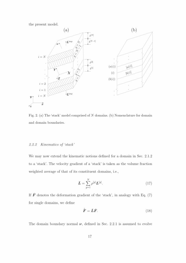
with a 2.27 GHz processor. Fig. 10 shows the wall clock computational time

per domain required to simulate tensile deformation up to strain ǫ22 = 1.0

and simple shear deformation up to strain ǫ12 = 1.0 using the E N models

of a polycrystal for N = 1, 2, 4, 8, 16 and 64. As expected, simulation times

increase with N as the models consider longer range intergranular interactions

with increasing N . Notably, however, computational times grow sub-linearly

with N . Also, computational times for any of the E N models considered is

41

0

2

4

6

8

10

12

14

10 20 30 40 50 60 70

N

Com

putation

time/ng[s]

tension (+)

simple shear (×)

Fig. 10. Total computational time per domain required to simulate tensile deforma-

tion to strain ǫ22 = 1 (+) and simple shear deformation to strain ǫ12 = 1 (×). Since

the data is noisy, smooth curves associated with each of the two data sets are also

shown to assist in their interpretation.

within a factor of four of the corresponding Taylor E1 model.

We also find that implementation of the consistency conditions described in

Sec. 2.2.5 reduces computational time substantially. This is because, enforcing

consistency reduces the degree of non-uniqueness, or often even eliminates

non-uniqueness of the solution. This extends the length of time steps of the

adaptive integration method used.

The reduction in computational time increases with increasing N . In simu-

lating tension to strain ǫ22 = 1.00, the computational time when enforcing

consistency is reduced by 0% for E 1, 19% for E 2, 21% for E 4, 22% for E 8

and 45% for E16 from its value without enforcing the consistency conditions.

No reduction is obtained in the Taylor case (E 1) because excepting special

orientations, the solution to the deformation problem is already unique.

42

6 Conclusion

A ‘stack’ model that accounts for intergranular interactions between N do-

mains abutting each other has been proposed. It extends the ‘ALAMEL’

models of Van Houtte et al. (2005) which treats interactions between pairs

of neighboring domains. Allowing for interaction between multiple domains

has been shown to reduce the constraint on individual domains, i.e., soften

the predicted stress-strain response, reduce the number of activated slip sys-

tems per domain. This produces qualitative and quantitative differences in

the predicted texture when used to simulate tensile and simple shear defor-

mations of a model two-dimensional polycrystal. All the observed responses,

both macroscopic and microscopic, saturate with increasing N . Furthermore,

the computational time associated with the present model increases only sub-

linearly with increasing N .

As stated in Sec. 1, successful multi-scale numerical simulations of deforma-

tion processes pose conflicting requirements of quantitative accuracy in the

predicted macroscopic response and microscopic state, as well as computa-

tional lightness of the micro-scale model. In the ‘stack’ model, the conflict

between these requirements appears to be within manageable limits. As seen

previously, for a specified degree of accuracy of the stress-strain and texture

response, an appropriate EN model capable of supplying response to that

accuracy can be identified whose computational cost will be well within an

order of magnitude of that required for the Taylor model. Although these con-

clusions have been arrived by studying a two-dimensional polycrystal, their

applicability to three-dimensional polycrystals also appears likely. The present

‘stack’ model is thus ideally suited for the purpose of supplying material point

43

response in simulations of macroscopic plastic deformation processes.

Acknowledgment: The authors thank the anonymous referees of this manuscript

for suggestions that helped improve it. Funding for this work was provided by

the Indira Gandhi Center for Atomic Research, Kalpakkam.

References

Aernoudt, E., Van Houtte, P., Leffers, T., 1993. Plastic Deformation and Frac-

ture of Materials. Vol. 6 of Materials Science and Technology: A Compre-

hensive Treatment. VCH, Ch. Deformation and textures of metals at large

strains, pp. 89–136.

Amirkhizi, A. V., Nemat-Nasser, S., 2007. A framework for numerical integra-

tion of crystal elasto-plastic constitutive equations compatible with explicit

finite element codes. Int. J. Plast. 23 (10-11), 1918–1937.

Anand, L., Kothari, M., 1996. A computational procedure for rate-

independent crystal plasticity. J. Mech. Phys. Solids 44 (4), 525–558.

Asaro, R., Lubarda, V., 2006. Mechanics of Solids and Materials. Cambridge

University Press.

Asaro, R. J., 1979. Geometrical effects in the inhomogeneous deformation of

ductile single crystals. Acta metall. 27 (3), 445–453.

Asaro, R. J., 1983. Micromechanics of crystals and polycrystals. In: Hutchin-

son, J. W., Wu, T. Y. (Eds.), Advances in Applied Mechanics. Vol. 23.

Academic Press, New York, Ch. 1, pp. 1–115.

Ashby, M. F., 1970. The deformation of plastically non-homogeneous materi-

als. Phil. Mag. 21 (170), 399.

Barbe, F., Decker, L., Jeulin, D., Cailletaud, G., 2001. Intergranular and in-

44

tragranular behavior of polycrystalline aggregates. part 1: F.E. model. Int.

J. Plast. 17 (4), 513–536.

Barrett, C. S., Levenson, L. H., 1940. Structure of aluminum after compression.

Trans. AIME 137, 112–127.

Barton, N. R., Knap, J., Arsenlis, A., Becker, R., Hornung, R. D., Jefferson,

D. R., 2008. Embedded polycrystal plasticity and adaptive sampling. Int.

J. Plast. 24 (2), 242–266.

Beaudoin, A. J., Dawson, P. R., Mathur, K. K., Kocks, U. F., 1995. A hybrid

finite element formulation for polycrystal plasticity with consideration of

macrostructural and microstructural linking. Int. J. Plast. 11 (5), 501–521.

Beaudoin, A. J., Mathur, K. K., Dawson, P. R., Johnson, G. C., 1993. Three-

dimensional deformation process simulation with explicit use of polycrystal

plasticity models. Int. J. Plast. 9 (7), 833–860.

Bishop, J. F. W., Hill, R., 1951. A theory of the plastic distortion of a poly-

crystalline aggregate under combined stresses. Phil. Mag. 42 (327), 414–427.

Bystrzycki, J., Kurzydlowski, K. J, Przetakiewicz, W., 1997. On the geometry

of twin boundaries and their contribution to the strengthening and recovery

of FCC polycrystals. Mater. Sci. Eng. A 225, 188-195.

Chin, G. Y., Mammel, W. L., 1969. Generalization and equivalence of the

minimum work (Taylor) and Maximum work (Bishop-Hill) Principles of

Crystal Plasticity. Trans. AIME 245, 1211.

Christoffersen, H., Leffers, T., 1997. The orientation of dislocation walls in

rolled copper relative to the crystallographic coordinate system. Scripta

mater. 37 (12), 2041–2046.

Cuitino, A. M., Ortiz, M., 1992. Computational modeling of single crystals.

Modelling Simul. Mater. Sci. Eng. 1, 225–263.

Engler, O., Crumbach, M., Li, S., 2005. Alloy-dependent rolling texture sim-

45

ulation of aluminium alloys with a grain-interaction model. Acta mater.

53 (8), 2241–2257.

Fleck, N. A., Ashby, M. F., Hutchinson, J. W., 2003. The role of geometrically

necessary dislocations in giving material strengthening. Scripta mater. 48,

179–183.

Fuh, S., Havner, K. S., 1986. On uniqueness of multiple-slip solutions in

constrained and unconstrained f.c.c. crystal deformation problems. Inter-

national Journal of Plasticity 2 (4), 329–345.

Ganapathysubramanian, S., Zabaras, N., 2005. Modeling the thermoelastic-

viscoplastic response of polycrystals using a continuum representation over

the orientation space. Int. J. Plast. 21 (1), 119–144.

Garmestani, H., Lin, S., Adams, B. L., Ahzi, S., 2001. Statistical continuum

theory for large plastic deformation of polycrystalline materials. J. Mech.

Phys. Solids 49 (3), 589–607.

Guan, Y., Pourboghrat, F., Barlat, F., 2006. Finite element modeling of tube

hydroforming of polycrystalline aluminum alloy extrusions. Int. J. Plast.

22 (12), 2366–2393.

Gurtin, M. E., 1981. An introduction to continuum mechanics. Academic

Press, New York.

Haddadi, H., Bouvier, S., Banu, M., Maier, C., Teodosiu, C., 2006. Towards

an accurate description of the anisotropic behaviour of sheet metals under

large plastic deformations: Modelling, numerical analysis and identification.

Int. J. Plast. 22 (12), 2226–2271.

Havner, K. S., 1992. Finite Plastic Deformation of Crystalline Solids. Cam-

bridge University Press.

Havner, K. S., Chidambarrao, D., 1987. Analysis of a family of unstable lattice

orientations in (110) channel die compression. Acta mech. 69 (1-4), 243–269.

46

Hill, R., 1961. Discontinuity relations in mechanics of solids. In: Sneddon, I. N.,

Hill, R. (Eds.), Progress in Solid Mechanics. Vol. 2. Interscience Publishers,

New York, Ch. 6, pp. 247–278.

Hill, R., 1966. Generalized constitutive relations for incremental deformation

of metal crystals by multislip. J. Mech. Phys. Solids 14 (2), 95–102.

Hirsch, J., Lucke, K., 1988a. Mechanism of deformation and development of

rolling textures in polycrystalline FCC metals: I Description of rolling tex-

ture in homogeneous CuZn alloys. Acta metall. 36 (11), 2863–2882.

Hirsch, J., Lucke, K., 1988b. Mechanism of deformation and development of

rolling textures in polycrystalline FCC metals: II Simulation and interpre-

tation of experiments on the basis of Taylor-type theories. Acta metall.

36 (11), 2883–2904.

Honneff, H., Mecking, H., 1978. A method for the determination of the active

slip systems and orientation changes during single crystal deformation. In:

Proc. 5th Int. Conf. on the Textures of Materials. Vol. 1. Springer-Verlag,

pp. 265–275.

Kalidindi, S. R., Bronkhorst, C. A., Anand, L., 1992. Crystallographic texture

evolution in bulk deformation processing of FCC metals. J. Mech. Phys.

Solids, 537–569.

Kalidindi, S. R., Duvvuru, H. K., 2005. Spectral methods for capturing crys-

tallographic texture evolution during large plastic strains in metals. Acta

mater. 53 (13), 3613–3623.

Kalidindi, S. R., Duvvuru, H. K., Knezevic, M., 2006. Spectral calibration of

crystal plasticity models. Acta Mater. 54 (7), 1795–1804.

Kanjarla, A. K., Van Houtte, P., Delannay, L., 2010. Assessment of plastic het-

erogeneity in grain interaction models using crystal plasticity finite element

method. Int. J. Plast. 26, 1220–1233.

47

Kim, J. H., Lee, M.-G., Barlat, F., Wagoner, R. H., Chung, K., 2008. An elasto-

plastic constitutive model with plastic strain rate potentials for anisotropic

cubic metals. Int. J. Plast. 24 (12), 2298–2334.

Knezevic, M., Kalidindi, S. R., Fullwood, D., 2008. Computationally efficient

database and spectral interpolation for fully plastic Taylor-type crystal plas-

ticity calculations of face-centered cubic polycrystals. Int. J. Plast. 24, 1264–

1276.

Kocks, U. F., Canova, G. R., 1981. How many slip systems, and which? In:

et al, N. H. (Ed.), Deformation of Polycrystals. Vol. 2. Riso National Lab-

oratory, Roskilde, Denmark, p. 135.

Kocks, U. F., Chandra, 1982. Slip geometry in partially constrained deforma-

tion. Acta Metall. 30 (3), 695–709.

Kocks, U. F., Tome, C. N., Wenk, H. R., 1998. Texture and Anisotropy. Cam-

bridge University Press, Cambridge, U.K.

Le, N. T., Havner, K. S., 1985. Analysis of tensile loaded f.c.c. crystals in 4-

and 8-fold symmetry. Mechanics of Materials 4 (1), 33–50.

Lebensohn, R., 1999. Modeling the role of local correlations in polycrystal

plasticity using viscoplastic self-consistent schemes. Modeling Simul. Mater.

Sci. Eng. 7, 739–746.

Lebensohn, R., Uhlenhut, H., Hartig, C., Mecking, H., 1998a. Plastic flow of γ-

TiAl-based polysynthetically twinned crystals: micromechanical modeling,

and experimental validation. Acta mater. 46 (13), 4701–4709.

Lebensohn, R. A., Turner, P. A., Signorelli, J. W., Canova, G. R., Tome,

C. N., 1998b. Calculation of intergranual stresses based on a large strain

visoplastic self-consistent polycrystal model. Modelling Simul. Mater. Sci.

Eng. 6, 447–465.

Lebensohn, R. E., Tome, C. N., 1993. A self-consistent anisotropic approach for

48

the simulation of plastic deformation and texture development of polycrys-

tals: application to zirconium alloys. Acta metall. mater. 41 (9), 2611–2624.

Lee, B. J., Ahzi, S., Parks, D. M., 2002. Bicrystal-based modeling of plasticity

in FCC metals. J. Eng. Mater. Tech. 124 (1), 27.

Lee, E. H., 1969. Elastic-plastic deformation at finite strains. J. Appl. Mech.

36, 1–6.

Leffers, T., 1975. On the misfit between the grains in a deformed sachs poly-

crystal and its relation to the inhomogeneous deformation of real polycrys-

tals. Scripta metall. 9, 261–264.

Leffers, T., 1978. The shortcomings of the Taylor model in the description of

the plastic deformation of real polycrystals. In: Proc. 5th Int. Conf. on the

Textures of Materials. Vol. 1. Springer-Verlag, pp. 277–287.

Leffers, T., Christoffersen, H., 1997. The importance of grain-to-grain inter-

action during rolling deformation of copper. Mater. Sci. Eng. A234–236,

676–679.

Liu, Q., Hansen, N., 1998. Macroscopic and microscopic subdivision of a cold-

rolled aluminium single crystal of cubic orientation. Proc. R. Soc. Lond. A

454, 2555–2592.

Loge, R. E., Chastel, Y. B., 2006. Coupling the thermal and mechanical fields

to metallurgical evolutions within a finite element description of a forming

process. Comput. Method. Appl. Mech. 195 (48-49), 6843–6857.

Mahesh, S., 2006. Deformation banding and shear banding in single crystals.

Acta mater. 54 (17), 4565–4574.

Mahesh, S., 2009. A hierarchical model for rate-dependent polycrystals. Int.

J. Plast. 25 (5), 752–767.

Mahesh, S., 2010. A binary tree based model for rate-independent polycrystals.

Int. J. Plast. 26 (1), 42–64.

49

Mahesh, S., Tome, C. N., McCabe, R. J., Kaschner, G. C., Beyerlein, I. J.,

Misra, A., 2004. Application of a sub-structure based hardening model to

copper under loading path changes. Metall Mater Trans A 35, 3763–3774.

Manonukul, A., Dunne, F. P. E., 2004. High- and low-cycle fatigue crack ini-

tiation using polycrystal plasticity. Proc. R. Soc. A 460 (2047), 1881–1903.

Mathur, K. K., Dawson, P. R., 1989. On modeling the development of crys-

tallographic texture in bulk forming processes. Int. J. Plast. 5 (1), 67–94.

Mika, D. P., Dawson, P. R., 1998. Effects of grain interaction on deformation

in polycrystals. Mater. Sci. Eng. A 257 (1), 62–76.

Molinari, A., Canova, G. R., Ahzi, S., 1987. A self consistent approach of the

large deformation polycrystal viscoplasticity. Acta metall. 35, 2983–2994.

Paul, H., Morawiec, A., Driver, J. H., Bouzy, E., 2009. On twinning and shear

banding in a Cu8 at.% Al alloy plane strain compressed at 77K. Int. J.

Plasticity 25, 1588–1608.

Peeters, B., Bacroix, B., Teodosiu, C., Houtte, P. V., Aernoudt, E., 2001a.

Work-hardening/softening behavior of bcc polycrystals during changing

strain paths: II TEM observations of dislocation sheets in an if steel dur-

ing two-stage strain paths and their representation in terms of dislocation

densities. Acta Mater. 49, 1621–1632.

Peeters, B., Seefeldt, M., Teodosiu, C., Kalidindi, S. R., Houtte, P. V.,

Aernoudt, E., 2001b. Work-hardening/softening behavior of bcc polycrys-

tals during changing strain paths: I An integrated model based on substruc-

ture and texture evolution, and its prediction of the stress-strain behavior

of an IF steel during two-stage strain paths. Acta Mater. 49, 1607–1619.

Pierce, D., Asaro, R. J., Needleman, A., 1983. Material rate dependence and

localized deformation in crystalline solids. Acta metall. 31 (12), 1951–1976.

Proust, G., Tome, C. N., Kaschner, G. C., 2007. Modeling texture, twinning

50

and hardening evolution during deformation of hexagonal materials. Acta

mater. 55, 2137–2148.

Radhakrishnan, K., Hindmarsh, A. C., 1993. Description and use of lsode, the

livermore solver for ordinary differential equations. In: Hindmarsh, A. C.

(Ed.), Lawrence Livermore National Laboratory. NASA reference publica-

tion, CA, USA, pp. 1–124.

Renouard, M., Wintenberger, M., 1981. Determination de l’amplitude des

glissements dans la deformation plastique homogene d’un monocristal sous

l’effet de contraintes et de diplacements imposes. C. R. Acad. Sci 283, 385–

388.

Rice, J. R., 1971. Inelastic constitutive relations for solids: An internal-variable

theory and its application to metal plasticity. J. Mech. Phys. Solids 19 (6),

433–455.

Sachs, G., 1928. Zur Ableitung einer Fliessbedingung. Z. Ver. Dtsch. Ing. 72,

734–736.

Taylor, G. I., 1938. Plastic strain in metals. J. Inst. Met. 62, 307.

Tome, C., Canova, G. R., Kocks, U. F., Christodoulou, N., Jonas, J. J.,

1984. The relation between macroscopic and microscopic strain hardening

in F.C.C polycrystals. Acta metall. 32 (10), 1637–1653.

Van Houtte, P., 1982. On the equivalence of the relaxed Taylor theory and the

Bishop-Hill theory for partially constrained plastic deformation of crystals.

Mater. Sci. Engng. 55, 69–77.

Van Houtte, P., Aernoudt, E., 1975a. Solution of the generalized Taylor theory

of plastic flow. I and II. Z. Metallkde. 66, 202–209.

Van Houtte, P., Aernoudt, E., 1975b. Solution of the generalized Taylor theory

of plastic flow. III Applications. Z. Metallkde. 66, 303–306.

Van Houtte, P., Delannay, L., Kalidindi, S. R., 2002. Comparison of two grain

51

interaction models for polycrystal plasticity and deformation texture pre-

diction. Int. J. Plast. 18 (3), 359–377.

Van Houtte, P., Delannay, L., Samajdar, I., 1999. Quantitative predictions of

the cold-rolling texture in low-carbon steel by means of the LAMEL model.

Texture microstruct 31 (3), 104–119.

Van Houtte, P., Kanjarla, A. K., Van Bael, A., Seefeldt, M., Delannay, L., 2006.

Multiscale modelling of the plastic anisotropy and deformation texture of

polycrystalline materials. Eur J Mech. A 25 (4), 634–648.

Van Houtte, P., Li, S., Engler, O., 2004. Modelling deformation texture of

aluminium alloys using grain interaction models. Aluminium 80, 702–706.

Van Houtte, P., Li, S., Seefeldt, M., Delannay, L., 2005. Deformation texture

prediction: from the Taylor model to the advanced lamel model. Int. J.

Plast. 21 (3), 589–624.

Van Houtte, P., Yerra, S. K., Van Bael, A., 2009. The facet method: A hierar-

chical multilevel modelling scheme for anisotropic convex plastic potentials.

Int. J. Plast. 25 (2), 332–360.

Wang, Z. Q., Beyerlein, I. J., LeSar, R., 2008. Plastic anisotropy in fcc single

crystals in high rate deformation. Int. J. Plast. 25 (1), 26–48.

52