7/23/2002

1

A STOCHASTIC PROGRAM FOR OPTIMIZING MILITARY

SEALIFT SUBJECT TO ATTACK

David P. Morton

Graduate Program in Operations Research

The University of Texas at Austin

Javier Salmerón

R. Kevin Wood

Operations Research Department

Naval Postgraduate School

19 July 2002

Abstract

We describe a stochastic program for planning the wartime, sealift deployment of military cargo subject to attack. The cargo moves on ships from US or allied seaports of embarkation through seaports of debarkation (SPODs) near the theater of war where it is unloaded and sent on to final, in-theater destinations. The question we ask is: Can a deployment-planning model, with probabilistic knowledge of the time and location of potential enemy attacks on SPODs, successfully hedge against those attacks? That is, can this knowledge be used to reduce the expected disruption caused by such attacks? A specialized, multi-stage stochastic mixed-integer program is developed and answers that question in the affirmative. Furthermore, little penalty is incurred with the stochastic solution when no attack occurs, and worst-case scenarios are better. In the short term, insight gained from the stochastic-programming approach also enables better scheduling using current rule-based methods.

1 Introduction

The United States Transportation Command (USTRANSCOM) is responsible for

planning the wartime deployment of US cargo ships, and their cargo, from US or allied seaports

of embarkation (SPOEs) to overseas seaports of debarkation (SPODs) (USTRANSCOM 2000).

This command uses little optimization to guide its planning for a deployment and, to our

knowledge, no stochastic optimization to accommodate uncertainty. The purpose of this paper is

(a) to develop a stochastic-optimization model that proactively plans for potential disruptions

caused by enemy attacks on SPODs, and (b) to illustrate the potential benefit of using such a

7/23/2002

2

model with realistic deployment data. Our model is designed to provide insight into tactical and

strategic issues associated with military sealift. A real-time operational tool would need to

capture more detail than the model we develop here.

1.1 The Problem

Military sealift deployments are driven by a flexible schedule of movement requirements

contained in the Time-Phased Force-Deployment Data (TPFDD). The TPFDD describes the

cargo needed in the deployment and the military units to which that cargo belongs, e.g., a Marine

Expeditionary Force or a Naval Mobile Construction Battalion. A typical timeframe for a

TPFDD is 100 days. The schedule includes time windows for when cargo will be available for

loading at the SPOEs, when it should pass through an SPOD, and when it should arrive at its in-

theater destination.

Currently, a TPFDD is planned using software tools like the Joint Flow and Analysis

System for Transportation (JFAST) (USTRANSCOM 2000). However, the emphasis in the last

few years has been on embedding such systems within a global command-and-control system so

that all cargoes and lift assets are visible to planners who must deal with contingencies “on the

fly.” Quick responses to contingencies are important, but JFAST is largely a rule-based system

that cannot optimize (or re-optimize) a schedule with respect to an objective such as “minimize

delay.” Furthermore, JFAST ignores the possibility of disruptions to the deployment caused by

enemy attacks.

The deterministic mixed-integer programs of Aviles (1995), Brown (1999) and others,

along with the deterministic version of the model described in this paper, address the lack of

optimization in existing sealift deployment-planning systems. Within the limits of modeling

approximations, these models provide an exact assignment and routing of ships to deliver the

TPFDD cargoes as best possible. The models typically minimize the ton-days of late cargo,

which are weighted in some fashion with respect to the amount of lateness.

7/23/2002

3

While a deterministic optimization model is potentially useful, it ignores the fact that an

enemy may disrupt the deployment by attacking the cargo-movement “network,” probably in

some forward area, i.e., near the SPODs. The potential for such disruptions is of increasing

concern within the US military (Joint Publication 3-11 2000, p. II-3). Attacks might be carried

out by mining harbors and/or shipping channels, or by attacking SPODs with missiles carrying

conventional, nuclear, chemical or biological warheads, or by terrorist attack. Therefore, our

main question is: Can we plan a sealift deployment while effectively hedging against the

potential disruption caused by attacks on our cargo-movement network in forward areas? Our

purpose is to convince planners that current planning tools can be improved: Not only should

these tools optimize, but they should also plan proactively for potential disruptions.

We build a multi-stage stochastic-programming model, called the “Stochastic Sealift

Deployment Model” (SSDM), to address these issues. SSDM can be modified to model many

types and locations of attacks, but we focus on biological attacks on SPODs, because SPODs

have been characterized as being particularly attractive targets for such attacks (Joint Publication

3-11 2000, p. III-30).

Biological weapons are not new, but their potential for serious military use has increased

in recent years (Cohen 1997, Defense Intelligence Agency 1998), and a biological attack on an

SPOD could certainly disrupt a deployment. Furthermore, biological weapons are inexpensive to

produce, and over a dozen of the United States’ potential adversaries may possess or may be

engaged in research on such weapons (Barnaby 1999, pp. 10-11). Thus, the threat must be taken

seriously. We assume that any biological attack is immediately detected, as would be the case

with biological warheads delivered by ballistic missile. This may not be a limiting assumption

because new detection systems are capable of quickly detecting biological warfare agents that

might be surreptitiously spread by terrorists or an enemy’s special operations forces. (For

example, see the papers in Leonelli and Althouse 1998.) An attacked SPOD will shut down

7/23/2002

4

entirely during a decontamination period, after which the port’s cargo-handling capacity will

come back to normal over a period of time, following some recovery schedule. The severity of

the attack, which may be uncertain, dictates the length of the decontamination period and the

recovery schedule. The state of the art in determining the potential damage caused by a

biological attack is not far advanced (Alexander 1999), but SSDM can be easily adjusted to

account for the latest information as it becomes available.

For simplicity, we assume at most one attack will occur during the deployment period,

although that attack may strike more than one SPOD. The timing, location(s) and severity of the

attack are uncertain and follow a probability distribution developed by intelligence reports and

planners. The single-attack assumption has one significant advantage: It enables us to model the

deployment using a special type of multi-stage stochastic program (e.g., Birge and Louveaux

1997, pp. 128-135), which is easier to solve than a model in which attacks could occur repeatedly.

This assumption is reasonable at this stage of study, because no current deployment-planning

models account for even a single attack, and because significant insight can be gained by studying

this case.

Other assumptions limit the scope of the work here: (a) Only a single generic cargo ship

is modeled, specifically, an American Eagle Roll-On/Roll-Off vessel carrying 15 ktons of cargo

(1 kton = 1,000 short tons = 907 metric tons), because this ship is typical of those used in

planning exercises (Military Traffic Management Command Transportation Engineering Agency

1994, Alexander 1999), and (b) airlift assets and airlift delivery requirements are ignored.

Conceptually, SSDM is easily extended beyond assumption (a) to incorporate a fleet of ships with

different cargo-handling characteristics (see Brown 1999), although the model would grow in size

and solution times would increase. Assumption (b) simply reflects the focus of the model. To a

large extent, airlift and sealift optimization may be considered separately because the mode of

transport for each cargo “package” is specified by the TPFDD and the two transportation

7/23/2002

5

networks share few resources. In the Persian Gulf War of 1991, sealift delivered about 85% of all

dry cargo, but airlift delivered most of the cargo in the early part of the deployment (Lund et al.

1993).

1.2 Stochastic Programming and Military Deployments

Stochastic programming has seen limited application in military deployment problems,

yet the study of related transportation problems under uncertainty reaches back to Ferguson and

Dantzig (1956). A notable early exception is an application of two-stage stochastic programming

for scheduling monthly and daily airlift with uncertain cargo demands (Midler and Wollmer

1969). Modest computational power has, presumably, impeded the application of similar

techniques to modern large-scale military mobility systems.

Currently, simulation is the preferred method of dealing with uncertainty in deployments.

The Warfighting and Logistics Technology Assessment Environment (WLTAE) links

warfighting and logistics simulation models into a single large simulation (Sinex et al. 1998).

The logistics modules of such simulations typically use rule-based methods like JFAST and have

limited, if any, capability for optimal re-scheduling after an attack. However, we note that Brown

(1999) does provide re-optimization techniques suitable for embedding in the WLTAE simulation

model. In particular, whenever a modeled disruption in the deployment takes place, his mixed-

integer program, or a faster heuristic, can re-schedule the next set of ships and cargoes to be

deployed.

A series of optimization models for planning sealift deployment has been developed at

the Naval Postgraduate School (Aviles 1995, Theres 1998, Alexander 1999, Brown 1999, Loh

2000). All of these contribute to our understanding of the problem, but all have significant

limitations. For instance, Theres (1998) ignores uncertainty; Aviles (1995) and Brown (1999)

plan using deterministic models that assume no disruptions will occur and then re-optimize after a

simulated disruption (an attack) does occur; Alexander (1999) and Loh (2000) have explicit

7/23/2002

6

stochastic models, but can handle only small problems and have unrealistic limitations on, or

relaxations of, post-attack recourse.

Deterministic airlift optimization models, analogous in concept to the above sealift

models, have been developed by Killingsworth and Melody (1995), Rosenthal et al. (1997) and

Baker et al. (2001). These linear programs model aircraft movements by continuous variables

rather than the integer variables with which we model ship movements. A continuous

approximation of many, relatively small, cargo aircraft is probably appropriate, but such an

approximation is inappropriate for fewer and much larger ships. Goggins (1995) and Niemi

(2000) have developed stochastic-programming variants of the deterministic optimization models

of Rosenthal et al. (1997) and Baker et al. (2001), respectively, to incorporate aircraft reliability.

Both models are stochastic programs with simple recourse (e.g., Ziemba 1974); in particular,

recourse amounts to paying a penalty for exceeding airbase capacity. So, unlike the model we

develop here, those models do not encompass dynamic re-routing. Mulvey and Vanderbei (1995)

and Mulvey and Ruszczynski (1995) describe a two-stage stochastic program, called “STORM,”

that assigns aircraft to routes in the first stage and, after realizing random point-to-point cargo

demands, assigns cargo to aircraft. In contrast to STORM, our scheduling paradigm does not

require an a priori commitment to the vehicle routing schedule over the entire planning period.

Powell et al. (2001) are currently developing techniques based on simulation and dynamic

programming to handle uncertainty in airlift deployments.

Sensitivity analysis, parametric programming, scenario analysis and other related ideas

are frequently (mis-)used in an attempt to determine the effect of uncertain parameters in an

optimization model. It is well known by stochastic programmers, but apparently less well known

in the general OR and military OR communities, that it is usually inappropriate to apply these

techniques to decision-making problems under uncertainty. Frequently, activities that provide

needed flexibility in a stochastic system are not utilized at all in the solution to the optimization

7/23/2002

7

problem under any single realization of the uncertain parameters, but these are exactly the kinds

of problems that sensitivity analysis, parametric programming and scenario analysis attempt to

exploit. Below, we discuss these issues in the context of two military stochastic-optimization

problems from the literature, and refer the reader to Wallace (2000) for a more general

discussion.

Whiteman (1999) investigates a network-interdiction problem with uncertain interdiction

effects using the following general approach: (a) He first solves the deterministic model, an

integer program, using mean values for uncertain parameters, (b) he then investigates the solution

for acceptability (sufficient reduction in expected network capacity) using Monte Carlo

simulation and (c) if it is unacceptable, he finds some near-optimal solutions to the deterministic

problem and performs the same objective-function estimation procedure until an acceptable

solution is found. The near-optimal solutions typically interdict more network components than

does the original solution and are therefore, intuitively, more robust to failed or partially

successful interdictions. While the technique may lead to a good solution that satisfies a specified

probabilistic criterion (e.g., expected capacity is reduced by at least 80%), there is no guarantee

that the solution is near-optimal. When the underlying problem is convex (e.g., a linear program),

convex combinations of candidate solutions are feasible and hence sometimes advocated. But

again, there is no guarantee that such an approach will yield an optimal, or even acceptable

solution.

Brooks et al. (1999) propose a technique they call “exploratory analysis” for solving what

are, essentially, stochastic-programming problems. A weapons-mix problem is provided as an

example. For motivation, they first solve a linear program to assign a given weapons mix (say,

1,000 weapons of type A, 2,000 of type B and 1,500 of type C) most effectively to a set of

targets. The potential target set is known, but the reliability of the weapons against those targets

is not. The linear program’s solution is correct only if those reliabilities are known.

7/23/2002

8

(“Reliability” is essentially the probability that the weapon will be successfully delivered to kill

the target.) The authors then show, using Monte Carlo estimation, that assuming expected

reliabilities for the weapons produces poor results and that applying standard sensitivity analysis

(e.g., Dantzig 1963, pp. 265-275) is futile. As an alternative technique, they propose exploratory

analysis, which (a) defines an exhaustive set of weapons mixes, (b) culls that set using “expert

knowledge” to eliminate obviously inferior solutions (c) simulates multiple scenarios of the

weapons’ reliabilities, (d) uses these scenarios to estimate the effectiveness of each candidate

weapons mix, and (e) selects the mix having the best sample average. (Initially, the authors

consider the results for a single theater or war, but later add scenarios with multiple theaters.) So,

using a brute-force enumerative technique, the authors find an arguably good solution to the

stochastic-programming problem: “Find the mix of weapons that is best, on average, across a

large set of reliability values for the weapons.” Standard stochastic-programming techniques

would probably lead to that solution, or a better one, more efficiently.

Stochastic programs, and particularly multi-stage stochastic programs, can be

computationally expensive to solve. That fact has probably played a role in leading analysts to

resort to the kind of approaches outlined above. Because the type of multi-stage stochastic

program we develop here has at most one uncertain event, it exhibits quadratic growth in the

number of time periods instead of the exponential growth characteristic of general multi-stage

problems. Infanger (1994, pp. 43-47) describes a different class of multi-period problems in

which capacity-expansion decisions with long lead-times result in what is effectively a two-stage

stochastic program. These problems grow linearly in size with the number of time periods.

Restricting, in some manner, the solution space is another commonly used technique to reduce

dimensionality of a multi-stage stochastic optimization problem. For example, in stochastic

dynamic programming, optimizing over the class of time-stationary policies can help yield

computationally tractable models (e.g., Bertsekas, 1987, Chap. 5). In a similar spirit, Mulvey et

7/23/2002

9

al. (2000) use nonlinear programming to search the class of “fixed-mix” investment policies in a

multi-period asset-liability management model; see also Fleten et al. (2000) and Gaivoronski and

de Lange (2000).

1.3 Outline of the Paper

In the remainder of this paper, we first describe SSDM in general terms, and then

mathematically. We then describe our simulation of current, rule-based planning methods, which

we compare to SSDM. We present computational results using data that represent a deployment

similar in scope to that of the Desert Shield/Desert Storm deployment of 1991. The last section

of the paper provides conclusions and points out areas for further development of SSDM.

2 The Stochastic Sealift Deployment Model (SSDM)

2.1 Introduction

This section provides a general and mathematical description of SSDM, which builds

upon similar models formulated by Alexander (1999) and Loh (2000). The model consists of

four main entities, a ship-movement sub-model, a cargo-movement sub-model, linking

constraints, and non-anticipativity constraints (Wets 1980).

The ship-movement sub-model routes a ship from an SPOE where it is loaded, to an

SPOD to be unloaded, and then back to an SPOE, not necessarily its originating port. But, it also

allows a ship to be re-routed from one SPOD to another in response to an attack, provided the

ship has not entered a berth, but is actually waiting just outside the SPOD. Ships nominally

require a fixed amount of time to unload their cargo, and they return to some SPOE immediately

after unloading is complete where they can be directly reloaded for another delivery, or wait until

needed. If an attack occurs during unloading, the unloading period is extended by the

decontamination period. For simplicity, ships become available for initial use according to a pre-

specified schedule, once the deployment commences. (Most of these ships are civilian, converted

7/23/2002

10

to military use for military contingencies, according to established agreements.) A more detailed

model might also incorporate uncertain availability of ships, and even breakdowns and weather-

related delays.

The cargo movement sub-model is similar to that for ship movement but incorporates

separate constraints for each commodity called a “cargo package.” It also adds an echelon of

variables to move cargo from the SPODs to the final destinations. This movement of cargo

would typically be accomplished by trucks or railcars, which are modeled through a single,

generic transportation mode. Side constraints control the movement of cargo out of the SPODs

and reflect cargo-handling capacity of the port in various situations: There is a nominal cargo-

handling capacity, but capacity goes to zero immediately after an attack and during

decontamination, and returns to its pre-attack level over a period of time after decontamination is

complete. Because of permanent losses to personnel, post-attack cargo-handling capacity might

never reach its pre-attack level, but this possibility is ignored for the sake of simplicity. (If the

post-attack capacity is assumed known, the model can be trivially modified to handle this. If this

capacity is uncertain, it simply adds scenarios to be considered.)

Linking constraints ensure that sufficient ship capacity is scheduled to carry the cargo

being moved from SPOE to SPOD, being re-routed between SPODs and being moved from

outside an SPOD into that port to be unloaded. Because cargo is not assigned to a specific ship,

the combination of linking constraints and flow-based sub-models does imply a relaxation of real-

world constraints. In particular, cargo can, in effect, move between ships that are waiting outside

an SPOD, but this does not occur in our computational examples.

The model’s variables and constraints are indexed by scenario, which encompasses the

time and location(s) of the attack, or indicates that no attack occurs. A solution to SSDM is said

to be implementable (Rockafellar and Wets 1991) if under any pair of scenarios a and a′, with

7/23/2002

11

attack times ta ≤ ta′, all decision variables associated with them are identical through time ta−1.

Non-anticipativity constraints ensure that this is the case.

The data set we analyze in this paper has two SPODs located in the Middle East, but our

assumption of a “single” attack allows a simultaneous attack on both SPODs or on either SPOD

and not the other. Scenarios could also encompass varying attack severity because of the

weapons used or environmental factors, which would translate into longer or shorter

decontamination periods and recovery schedules. For simplicity, this severity is fixed in our

computations.

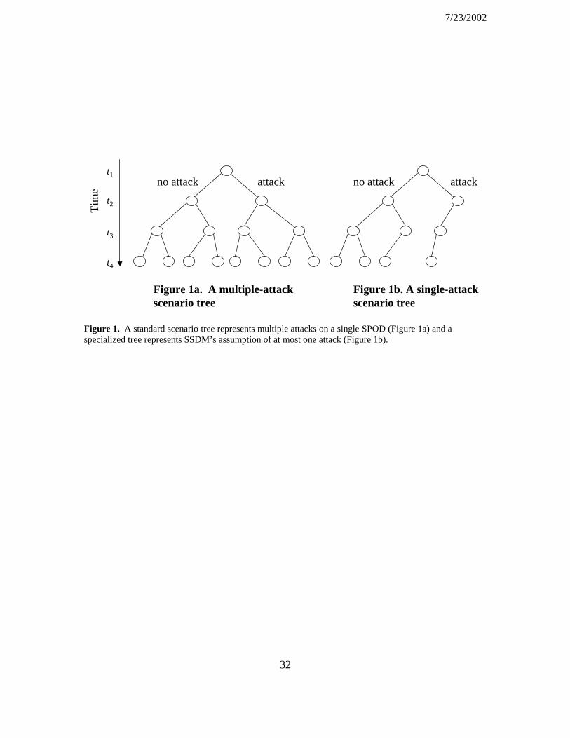
The fact that we consider only a single attack substantially reduces the size of our multi-

stage stochastic program. Figure 1a shows a typical multi-stage scenario tree in which, after the

first period, an attack may occur in any time period (at a given SPOD, say) during a four-period

horizon and may occur any number of times. For instance, the left-most leaf of the tree

represents the “no-attack scenario” and the right-most leaf represents the “attack-in-every-time-

period scenario.” Figure 1b illustrates the scenario tree that represents the simplifying

assumption of SSDM in which at most one attack will occur. (The actual scenario trees for

SSDM are somewhat more complicated because of multiple attack types.) The number of nodes

and scenarios in the tree of Figure 1a grows exponentially with the number of stages while, in

Figure 1b, the number of nodes grows quadratically and the number of scenarios grows linearly.

2.2 Mathematical Description of SSDM

The mathematical description of SSDM follows a standard format for mathematical

programs except that indices, sets and data are divided into deterministic and stochastic groups.

All model elements that depend on the scenario index a are deemed “stochastic.”

Deterministic Indices and Index Sets

e E∈ Seaports of embarkation (SPOEs)

7/23/2002

12

d D∈ Seaports of debarkation (SPODs) f F∈ Final destinations (geographic locations where cargo is delivered)

c C∈ Cargo packages, i.e., cargo moving from the same SPOE to the same final destination

with identical available-to-load dates, and required delivery dates

( )e c Fixed, originating SPOE for cargo package c

( )f c Fixed, final destination for cargo c t T∈ Time periods, T = {1,…,tmax+1 } (nominally days); tmax is the end of the time horizon

and tmax+1 is a dummy time period

( )e cT T⊆ Allowable shipping periods for cargo c from SPOE e(c) (depends on cargo

availability dates, shipping delays and latest acceptable delivery date)

Stochastic Indices and Index Sets

a A∈ Attack scenarios. In addition to timing, the scenario contains the information on the SPOD or SPODs attacked, and could contain the post-attack decontamination time and recovery schedule. This set also includes the “no-attack scenario” denoted a0

at Attack time of scenario a ( max1 at t< ≤ ) for 0a a≠ ; 0 max 1at t= +

TTa ⊆ Time periods that run from the first period up to but not including the attack time for

scenario a, i.e., {1, , 1}a aT t= −…

dtaT T⊆ Set of periods t ′ such that if a ship enters SPOD d at time t ′ then it will still occupy

a berth there at time t (depends on unloading time and any necessary decontamination)

*

daT T⊆ Time periods, if any, during which SPOD d remains contaminated under scenario a

(computed using ta defined above, and δUdta defined below)

Deterministic Data

1edδ One-way travel time from SPOE e to just outside SPOD d (time periods)

2deδ One-way travel time from SPOD d to SPOE e (time periods)

3

dd ′δ One-way travel time from just outside SPOD d to just outside SPOD d ′ (time

periods)

7/23/2002

13

Fdfδ Travel time from SPOD d to destination f (time periods)

ALDcτ Available-to-load date for cargo c. This is the earliest date (time period) the cargo is

available at its SPOE for loading

CRDcτ Required delivery date (CRD) for cargo c at its final destination f(c) (time period)

MAXδ Cargo delivered later than MAXCRD

cτ δ+ is considered unmet demand for any type of

cargo (time periods)

( , )c dτ − Earliest-possible-arrival date (time period) for cargo c at its destination f(c) given that

it travels through SPOD d; computed using ALDcτ , 1

( ),e c dδ and F, ( )d f cδ

( )cτ + Latest-possible-arrival date (time period) for cargo c at its destination f(c); defined as MAXCRD

cτ δ+

cdtLPEN Late-delivery penalty (penalty units/ton) for cargo c leaving SPOD d in period t. The

penalty is based on the difference between actual and required delivery dates:

{ }F, ( )max 0, ( )CRD

cdt d f c cLPEN tα

δ τ = + − . The exponent satisfies 0α > , with

1α > used in practice

cUPEN Penalty for not delivering a required ton of cargo c within its required time window

(penalty units/ton); { },maxc d t cdtUPEN LPEN>

1ε Small penalty to discourage unnecessary ship voyages (penalty units/ships)

2ε Small penalty to discourage unnecessary re-routing of ships (penalty units/ships) XTOTc Total amount of cargo c required (tons) VCAP Capacity of a ship (tons) VBERTHd Berthing capacity at SPOD d (ships) VINVet Number of ships entering inventory at SPOE e at time t (ships)

7/23/2002

14

Stochastic Data

δUdta Unloading time for a ship that enters SPOD d in period t under scenario a (time

periods); includes decontamination time if an attack occurs during unloading. Since ships are not allowed to enter an SPOD during decontamination, this parameter is

defined only for *daTTt −∈

XCAPdta Capacity of SPOD d to handle cargo at time t under scenario a (tons/time period); the

nominal capacity drops to zero after an attack and during decontamination, and slowly returns to its nominal or near-nominal level after decontamination

aφ Probability that scenario a occurs

Variables

Under scenario a:

etavi Number of ships in inventory at SPOE e at time t

edtavs Number of ships starting voyages from SPOE e to SPOD d at time t

dtavb Number of ships at waiting area outside SPOD d at time t

dd tavrr ′ Number of ships re-routed from SPOD d to SPOD dd ≠′ at time t

dtavh Number of ships entering berth at SPOD d at time t

detavr Number of ships returning from SPOD d to SPOE e at time t

cdtaxs Tons of cargo c shipped at time t from SPOE ( )e c to SPOD d

cdtaxb Tons of cargo c at waiting area outside SPOD d at time t

cdd taxrr ′ Tons of cargo c re-routed from SPOD d to SPOD dd ≠′ at time t

cdtaxh Tons of cargo c entering berth at SPOD d at time t

cdtaxi Tons of cargo c in inventory at SPOD d at time t awaiting shipment to its final

destination f(c)

7/23/2002

15

cdtaxw Tons of cargo c transported to its destination f(c) from SPOD d at time t

caxu Tons of unmet demand for cargo c

Formulation

minimize a cdt cdta a c caa c d t a c

LPEN xw UPEN xuφ φ+∑∑∑∑ ∑∑

1 2a edta a dd taa e d t a d d d t

vs vrrε φ ε φ ′′≠

+ +∑∑∑∑ ∑∑∑∑ (1)

subject to:

21 , ,, ,

deet a edta eta etde t a

d d

vi vr vs vi VINV e t aδ− −− − + + = ∀∑ ∑ (2)

1 31, , , , 0 , ,

ed d ddta dta dt a dd taed t a d d t a

e d d d d

vh vs vb vb vrr vrr d t aδ δ ′′− ′− −

′ ′≠ ≠

− + − + − = ∀∑ ∑ ∑ (3)

*

, ,0 , ,U

dtadta dade t a

e

vh vr d a t T Tδ+− + = ∀ ∈ −∑ (4)

, ,dta

dt a dt T

vh VBERTH d t a′′∈

≤ ∀∑ (5)

*0 , ,dta davh d a t T≡ ∀ ∈ (6)

*0 , ,deta davr d a t T≡ ∀ ∈ (7)

( )

,e c

cdta cd t T

xs XTOT c a∈

≤ ∀∑ ∑ (8)

1 3( )

1, , , ,0 , , ,

e c d d dcdta cdta cdt a cdd tacd t a cd d t a

d d d d

xh xs xb xb xrr xrr c d t aδ δ ′′− ′− −

′ ′≠ ≠

− + − + − = ∀∑ ∑ (9)

, , , 1, , ,0 , , ,U U U

dta dta dtacdta cd t a cd t a cd t a

xh xi xi xw c d t aδ δ δ+ + − +− + − + ≤ ∀ (10)

, ,cdta dtac

xw XCAP d t a≤ ∀∑ (11)

, ( )

, ( )

( )

( , )

,

Fd f c

Fd f c

c

cdta ca cd t c d

xw xu XTOT c aτ δ

τ δ

+

−

−

= −

− − = − ∀∑ ∑ (12)

| ( )

0 , , ,cdta edtac e c e

xs VCAP vs e d t a=

− ≤ ∀∑ (13)

7/23/2002

16

0 , , ,cdd ta dd tac

xrr VCAP vrr d d d t a′ ′ ′− ≤ ∀ ≠∑ (14)

0 , ,cdta dtac

xh VCAP vh d t a− ≤ ∀∑ (15)

All variables are non-anticipative, e.g.,

, , ,eta eta a avi vi e a a t T T′ ′′= ∀ ∈ ∩ (16)

All variables are non-negative (17)

Ship variables are integer: , , , , ,eta edta dta dd ta dta detavi vs vb vrr vh vr′ (18)

Any variable with a time index not in T is fixed to 0, e.g.,

aTtdddvrr tadd ,,,0 ∉≠′∀≡′ (19)

2.3 Description of the Formulation

The basic premise of the model is to meet demands for cargo of various types during

specified delivery time windows, although this will probably not be possible given limited system

capacities, especially after attacks. This component of the objective function (1),

cdt cdta c cac d t c

LPEN xw UPEN xu+∑∑∑ ∑ , (20)

measures the disruption associated with scenario a. The first term corresponds to late deliveries

with the per-ton penalty cdtLPEN , which will increase as the function τα, where α is a strictly

positive parameter and τ is the number of periods the cargo is late. We typically use α > 1 to

express, roughly, “One ton of cargo late for t periods is worse than t tons of cargo late for one

period.” The second term in (20) strongly penalizes cargo not arriving during an acceptable

delivery window: Such cargoes are absorbed as unmet demand with a penalty that is higher than

for the latest acceptable delivery. Therefore, ignoring the last two terms of (1), this objective

function measures the total expected disruption for a deployment plan. We note that large

inventories of early-arriving cargo could be vulnerable to attack, but within the scope of our

7/23/2002

17

model, explicit penalties are unnecessary to handle this. If early-arriving cargo is vulnerable, it

ends up being delayed in one or more attack scenarios and is therefore penalized appropriately.

The last two terms of the objective function are small factors to eliminate unnecessary ship

movements.

The ship-movement sub-model is represented by constraints (2)-(7) and associated

variables. The cargo-movement sub-model is represented by constraints (8)-(12) and associated

variables. Constraints (13)-(15) link the two sub-models and constraints (16) account for non-

anticipativity, which ensure implementability of the decision variables with respect to the various

scenarios. Note that, although these constraints are written for every pair ),( aa ′ , it suffices to

enforce them for appropriately defined pairs of “consecutive scenarios.”

Of course, all variables are non-negative and the ship variables are required to be integer;

see constraints (17) and (18), respectively. Additionally, variables with time indices outside of T

do not represent true model entities and must be fixed to 0; see constraints (19).

Constraints (2) are ship-supply constraints for each SPOE. The supply of ships at time t

includes those ships that become available via etVINV according to a pre-designated plan which

does not depend on the scenario a (but could if desired); it includes those ships that have returned

from earlier deliveries ( 2, ,dede t avr δ−

); and it includes those ships that have previously been put into

“inventory” at the SPOE awaiting assignment ( 1et avi − ). The supply of ships is used to deliver

cargo ( edtavs ) or is held in inventory ( etavi ).

Constraints (3) are flow-balance constraints for the ships just outside the SPODs. A ship

can arrive from an SPOE ( 1, ,eded t avs δ−

) or by being re-routed from another SPOD ( 3, ,d dd d t avrr δ ′′ −

). A

ship that arrives can “park” outside the SPOD waiting for an available berth ( dtavb ), it can enter

the SPOD and berth ( dtavh ), or it can be re-routed to an alternate SPOD ( dd tavrr ′ ).

7/23/2002

18

Constraints (4) ensure that a ship entering an SPOD ( dtavh ) does not leave and return to

an SPOE (, ,U

dtade t avr δ+

) until it has time Udtaδ to unload, and decontaminate if necessary.

Constraints (5) ensure that berthing capacity is not exceeded by the ships that have entered the

SPOD. Constraints (6) and (7) ensure that no ships enter or leave a contaminated SPOD.

Constraints (8) are supply constraints for cargo; they are inequality constraints because,

under certain scenarios, it can be determined that certain cargo cannot reach its destination within

the allotted time window, so it will not be shipped. Constraints (9) balance flow of cargo just

outside the SPODs, analogous to constraints (3) for ships.

Constraints (10) are inequality versions of flow-balance constraints for cargo inside the

SPOD. Cargo that enters the SPOD, at time t ( cdtaxh ) becomes available to enter inventory

(, ,U

dtacd t axi δ+

) or be shipped out to its final destination (, ,U

dtacd t axw δ+

) after it has been unloaded, and

possibly decontaminated, at time Udtat δ+ . Cargo in inventory from an earlier unloading is also

available for shipment (, 1,U

dtacd t axi δ+ −

). These constraints are inequalities because it is possible for

cargo to arrive so late, or be trapped for decontamination inside the SPOD so long, that it cannot

reach its final destination in time to be of any value. Such cargo is unloaded at the SPOD and is

subsequently ignored by the model.

Constraints (11) limit shipments of unloaded cargo out of the SPOD depending on that

SPOD’s cargo-handling capacity. There is a nominal capacity for each SPOD, which becomes

zero immediately after an attack, i.e., during decontamination. The capacity then increases

toward the nominal capacity during a post-decontamination period following some recovery

schedule. Constraints (12) are simply the demand constraints for each cargo, with variables caxu

absorbing unmet demand.

7/23/2002

19

Constraints (13)-(15) ensure that cargo is transported only if there is sufficient

capacity on the ships that must move that cargo. These constraints cover cargo moving from

SPOE to SPOD, from one SPOD to another, and from just outside an SPOD into its docks.

3 Simulating Rule-Based Planning

Ideally, we would like compare deployment plans developed through optimizing SSDM

to plans developed through current rule-based planning methods. SSDM explicitly incorporates

and evaluates the total expected disruption across all scenarios, but to evaluate rule-based

planning we would have to perform the following steps for a given “test case,” i.e., combination

of data and probability distributions for when and where potential attacks might occur:

1. Use rules to create a baseline deployment plan, “Plan0,” under the no-attack

scenario a0.

2. For each scenario a ≠ a0: Evaluate the cargo movements using Plan0 up to the

time of the attack, simulate the disruption caused by the attack, and then plan the

(re-) deployment of ships and cargo from the attack time onward using a rule-

based procedure.

3. Compute the total expected disruption using the disruption values computed

above and the given probability distribution.

We cannot perform the above procedure exactly because no actual deployment-planning

software is available to us. However, we can simulate that procedure by replacing rule-based

plans with optimization-based plans. In particular, Plan0 is determined by solving a single-

scenario variant of SSDM under the no-attack scenario—call this model DSDM(a0). The

redeployment is determined through another single-scenario model running from ta through the

end of the horizon given the simulated effects of an attack at time ta—call this model

DSDM(a|a0). The entire procedure, or “deterministic heuristic,” is denoted DSDH.

7/23/2002

20

In some of our test cases, attacks can only occur late in the time horizon and it seems that

planners could probably take this information into account to make the rule-based deployment

plan more robust against attack. In such cases, common sense dictates that we push the cargo

through the system as quickly as possible so as to minimize the amount that is susceptible to

attack in later time periods. We modify DSDM(a0) to reflect this by adding a negative penalty

(i.e., a benefit) into the objective function for early cargo arrivals. In particular, if one ton of

cargo package c whose required delivery date is CRDcτ actually arrives in period t < CRD

cτ , it incurs

a “penalty” of ( )CRDc t αβ τ− − , for some 0β > , but if it arrives after CRD

cτ , it incurs the usual

penalty of ( )CRDct ατ− . Model DSDM(a0) with this modification is denoted DSDM′(a0), and the

overall deterministic heuristic that uses this initial model is denoted DSDH′.

We have found that a single small value of β will yield solutions to DSDM′(a0) that are

optimal with respect to the original objective of DSDM(a0), but do push cargo through more

quickly. Thus, there are multiple optimal solutions to DSDM(a0) and we are taking advantage of

that fact. In effect, we are solving the goal program that (a) optimizes one objective, i.e., it

minimizes disruption, (b) adds a constraint that requires all solutions be optimal with respect to

that objective value, and (c) then optimizes a secondary objective of pushing cargo through

quickly.

By using DSDH′, we are trying to find an acceptable solution to our stochastic program

from among multiple-optimal deterministic ones, yet in the introduction we warned that this

might be impossible. However, if it is possible at times, we will be satisfied that we have (a)

provided a stochastic-programming baseline for validating current methods, and (b) improved

those methods in the short term. We can still argue that those methods should be replaced in the

long term, and we will do this with computational results at hand in the next section.

7/23/2002

21

Complementing our rule-based planning methods, we devise a procedure to compute a

lower bound z+ on the optimal objective value of SSDM. We call this procedure D+. The value z+

is computed by solving, for each a A∈ , DSDM(a), which is the deterministic version of SSDM

with the effect of the scenario a attack incorporated. The expected disruption computed over all

scenarios is z+. This is a lower bound—it is an example of the well-known “wait-and-see bound,”

e.g., Birge and Louveaux (1997, p. 138)—because in each scenario the optimizing planner is

assumed to know if and when an attack will occur.

4 Computational Results

This section describes the computational results for SSDM, DSDH, DSDH′, and D+. All

computation is performed on a 1.7 GHz dual-processor Pentium IV computer with 2 Gb of RAM,

running under Microsoft Windows 2000. Models are generated using GAMS (Brooke et al.

1996) and solved using CPLEX Version 7.0 (ILOG 1999), with a 1% relative optimality

tolerance.

4.1 Data

The data describe a hypothetical deployment to the Middle East requiring the movement

of about 3,000 ktons of cargo, in 11 different packages, over the course of 100 days aggregated

into 50 two-day time periods. The cargo is required between periods 7 and 45 of the deployment

and the maximum-lateness parameter MAX( )δ is 7 periods. There are four SPOEs in the United

States and Europe and there are two SPODs, denoted d1 and d2, in close proximity to each other

in the Middle East. The travel time between SPOEs and SPODs ranges from 6 to 12 periods.

158 ships become available to load cargo according to a pre-specified schedule over the course of

the first 15 periods. Each ship can transport up to 15 ktons of cargo per trip. This hypothetical

deployment is similar in scope to the one executed under Operation Desert Shield/Desert Storm in

1990 and 1991 (Alexander 1999).

7/23/2002

22

Each SPOD has berth capacity for at most nine ships at a time. Under normal conditions,

a ship is unloaded in two periods and the port has 150 ktons/period of cargo-handling capacity to

forward that cargo on to its final destination. Any attack on an SPOD, however, will close the

port for a number of periods for decontamination, during which the cargo-handling capacity is

lost entirely and the unloading process is halted. Decontamination commences immediately after

the attack and, upon completion, ships continue to unload at their standard rate. However, other

cargo-handling capacity at the port only returns to normal gradually, according to a given

recovery schedule. We consider a fixed decontamination period of 7 periods with capacity

recovering at a rate of 25% per period after decontamination. These values could be part of

scenario definitions in a more detailed model.

The objective function of SSDM, equation (1), measures total expected disruption (see

Section 2.3) to the deployment. Disruption resulting from late deliveries is measured in terms of

“weighted kton-periods.” Specifically, k ktons of cargo that are τ periods late incur a penalty of

k×τ 1.5. Disruption resulting from an unmet delivery of k ktons of cargo from package c is

1.5ck τ× , where cτ is a strict upper bound on the number of periods late that package c is still

considered worth delivering.

4.2 Test Cases and Results

In the following, we analyze the benefits of the stochastic solution using combinations of

attack types and probability distributions we call test cases. In practice, analysts would develop

these from intelligence reports. The attack types are:

S={ }}{}{ 21 d,d : An attack occurs at SPOD d1 or at SPOD d2, but not both, or no attack

occurs;

S={ }}{}{ 211 d,d,d : Mutually exclusively, an attack occurs at 1d , both SPODs are

attacked simultaneously, or no attack occurs; or

7/23/2002

23

S={ }1 2 1 2{ },{ },{ , }d d d d : Mutually exclusively, 1d is attacked, 2d is attacked, both 1d

and 2d are attacked simultaneously, or no attack occurs.

The probability distributions for the test cases are defined by (a) the probability of no

attack, 0

0.5aφ = , (b) by the assumption that in any given period, an attack of any element of S is

equally likely, and (c) the following conditional distributions for the timing of an attack:

U1: Uniform distribution over periods 4 through 40,

T1: Triangular distribution over periods 4 through 40 with mode 22,

U2: Uniform distribution over periods 4 through 18,

T2: Triangular distribution over periods 4 through 18 with mode 11,

U3: Uniform distribution over periods 26 through 40, and

T3: Triangular distribution over periods 26 through 40 with mode 33.

The first distribution, U1, is the “baseline distribution” accounting for almost no

information. T1 employs the same range of periods but gives more likelihood to attacks

occurring in the middle of the deployment. U2 and T2 represent a situation in which planners

believe the enemy will strike early in the deployment: Perhaps the enemy believes, and our

intelligence suggests, that early strikes will have a strong psychological effect against us and

compound our scheduling problems in a way that a later strike would not. U3 and T3 represent

the anticipation of late strikes: Perhaps intelligence reports indicate that the enemy will

experience some delay in deploying his biological weapons.

Table 1 describes the set of test cases and associated model statistics. Table 2 displays

the computational results for the test cases under the various models and solution procedures:

SSDM, DSDH and DSDH′, as well as the lower-bound procedure D+.

7/23/2002

24

The SSDM column of Table 2 reports the total expected disruption, i.e., objective

function value, for the stochastic model applied to each test case. All solutions are within 1% of

optimal and solution times are displayed in parentheses, in elapsed seconds.

In summary, the results show that

1. SSDM reduces total expected disruption over the simulated rule-based planning

of DSDH by an average of 22% with a range of 1% to 47%. With respect to the

improved heuristic DSDH′, SSDM reduces expected disruption by an average of

8%, with a range of 1% to 14%.

2. Even though DSDH′ was intended to improve results with late attacks (U3 and

T3), it also performs well relative to DSDH when the attack can occur over the

widest range of periods (U1 and T1). Under early attacks (U2 and T2), DSDH

outperforms DSDH′, but all such differences are small, i.e., at most 0.3%; thus,

we only discuss DSDH′ in what follows.

3. The lower bound provided by D+ is below the near-optimal solution value of

SSDM by an average of 20%. This indicates that even if DSDH′ does provide a

good solution, we still must solve SSDM to verify its quality.

4. Early-attack cases leave the least flexibility for the stochastic program to improve

upon rule-based planning. The average reduction in disruption of SSDM over

DSDH′ is 3%, with a range of 1-6% for the six U2 and T2 cases.

5. Conversely, the stochastic program has the greatest leverage when attacks can

only occur late in the deployment. The analogous average and range for the six

U3 and T3 cases are 11% and 7-13%. Finally, the range and average for the U1

and T1 cases are 8% and 5-11%.

We explain the general dominance of DSDH′ over DSDH (result 2 above) as follows:

Even if attacks can occur at any time, it makes sense to push cargo through the system as quickly

7/23/2002

25

as possible because, if an attack occurs, delayed cargo has as much slack time as possible to reach

its destination. However, pushing cargo quickly is a “double-edged sword”: The higher

disruption for DSDH′ compared to SSDM is largely explained by the fact that DSDH′ moves

cargo too fast to the SPODs in a few scenarios, and a large quantity becomes trapped in the

attacked SPOD in those scenarios and cannot reach its destination in time. SSDM better balances

the speedy arrival of cargo against the flexibility to reroute cargo waiting outside an SPOD that

may be attacked.

Table 3 helps investigate the behavior of the various procedures under likely and

especially disruptive scenarios. Since the no-attack scenario is likely to occur, we want to know

if the solutions from the stochastic model are robust in this scenario. The table shows that they

are. The table also shows that the worst-case scenarios for the stochastic model are usually less

disruptive than the worst-case scenarios for rule-based planning.

The results above seem to indicate that the stochastic-programming approach can yield

substantial improvements over rule-based planning, which is represented by a tuned deterministic

optimization model (arguably an optimistic representation of rule-based planning). It is important

to understand when the need for using a model such as SSDM is most acute. As described above,

when SSDM has the most time prior to the attack to hedge (i.e., the U3 and T3 distributions), the

value of the stochastic solution is the largest. We test this sensitivity with respect to the

distribution governing the time of attack by considering a triangular distribution, denoted T3′, in

which we change the mode of the triangular distribution from 33 to 40. The associated

computational results for each of the three attack types are shown in Table 4. The expected

disruption of SSDM’s solution is better than that of simulated rule-based planning by 25%, 14%,

and 13% for the three types of attack; these values have increased from 8%, 13%, and 10%,

respectively, for the original T3 distribution. These results are consistent with the trend in Table

7/23/2002

26

3 of SSDM solutions becoming more valuable as we move from early attack times, to the widest

range of attack times, to late attack times.

5 Conclusions

This paper has devised a specialized, multi-stage stochastic mixed-integer

programming model for planning the delivery of sealift cargo in a wartime deployment,

subject to possible enemy attacks on one or more seaports of debarkation (SPODs). The

attacks are simulated by halting berthing, unloading and other cargo handling until

decontamination is complete; the timing and location of the attack are uncertain. Once

decontamination is complete, post-attack cargo-handling capacity of the SPOD gradually

returns to normal. We focus on the effects of biological attacks, but the model could be

modified for conventional, nuclear or chemical attacks.

The stochastic program SSDM and two (simulated) rule-based planning schemes

have been tested with data from a realistic wartime deployment with 158 ships becoming

available at different times during the deployment, 11 cargo types, four seaports of

embarkation where cargo is loaded and two SPODs where cargo is unloaded before

reaching its final destination. Our test cases assume there is a substantial probability of no

attack, but if an attack does occur, it occurs with known probability distribution for timing

and location.

Expected cargo lateness, measured in weighted ton-periods, improves by up to

25%, depending on data and probabilistic assumptions, when compared to expected results

obtained using a simulation of current, rule-based planning techniques. (In fact, we

compare against a “tuned” rule-based technique that is rooted in a deterministic

optimization model and may overestimate how good rule-based techniques can be; hence,

7/23/2002

27

our comparisons are conservative.) However, there is little price to pay in terms of cargo

lateness for the stochastic solution if no attack occurs. In conclusion, hedging against a

possible attack can provide substantial benefits if an attack occurs, and incurs only minor

penalties if not.

Our simulations of current rule-based plans have shown that it may be possible to

establish rules that are more robust against potential attacks early in the deployment

horizon, without using a special stochastic-programming model. In these cases, SSDM

improves over rule-based planning, designed to push cargo through the system as quickly

as possible, by only an average of 3%. However, this contrasts with larger averages of 8%

when an attack may occur at almost any time (uniform distribution for attack time), and

11% and 17% for two sets of late-attack distributions. Except in the case of early attack, it

may be impossible to adjust a rule-based system to behave nearly as well as a stochastic

one. Furthermore, it is probably impossible to know how well rule-based planning is

performing without an optimal, stochastic solution to serve as a baseline lower bound.

(One standard lower bound is very weak.) So, rule-based systems can be improved, but

the stochastic-programming approach will ultimately be superior.

The current emphasis in the US military’s deployment planning is for providing

up-to-the-minute tracking of all cargo and transportation assets, with the ability to quickly

respond to contingencies. This is no doubt important, but planners can expect more timely

arrival of cargo into a theater of war if they proactively plan for those contingencies.

Further testing and development of SSDM is warranted. The model should be

tested against wartime deployment situations in other parts of the world. Conceptually,

the model is easy to expand for other sources of uncertainty such as the location of the

cargo-carrying ships when deployment planning is commenced. Also, SSDM currently

assumes that if an attack occurs during the deployment, there will only be one, although it

7/23/2002

28

may affect more than one SPOD: The model should, of course, be expanded to consider

more than one attack, but this will be require more general, multi-stage stochastic-

programming models and solution techniques.

6 Acknowledgements

The authors would like to thank the students at the Naval Postgraduate School whose

research has provided the foundation for our work: Tammy Glaser, Steven Aviles, Michael

Theres, Christopher Alexander and Loh Long Piao. David Morton’s research was supported by

the National Science Foundation through grant DMI-9702217 and the State of Texas Advanced

Research Program through grant #003658-0405-1999. Javier Salmerón’s research was supported

by a National Research Council Postdoctoral Fellowship. Kevin Wood’s research was supported

by the Office of Naval Research and the Air Force Office of Scientific Research. The authors

thank all of their supporting agencies.

7/23/2002

29

7 References

Alexander, C., 1999. “Effects of Biological Warfare on Throughput at Seaports of Debarkation during a Major Theater War,” M.S. Thesis in Operations Research, Naval Postgraduate School, Monterey, CA, September.

Aviles, S., 1995. “Scheduling Army Deployments to Two Nearly Simultaneous Major Regional Conflicts,” M.S. Thesis in Operations Research, Naval Postgraduate School, Monterey, CA, September.

Baker, S.F., Morton, D.P., Rosenthal, R.E. and Williams, L.M., 2002. “Optimizing Military Airlift,” to appear in Operations Research.

Barnaby, W., 1999. The Plague Makers: The Secret World of Biological Warfare, Vision Paperbacks, London.

Bertsekas, D.P., 1987. Dynamic Programming: Deterministic and Stochastic Models, Prentice-Hall, Inc., Englewood Cliffs, New Jersey.

Birge, R. and Louveaux, F., 1997. Introduction to Stochastic Programming, Springer Series in Operations Research, Springer-Verlag, New York.

Brooke, A., Kendrick, D. and Meeraus, A., 1996. GAMS, A User's Guide, GAMS Development Corporation, Washington, DC.

Brooks, A., Bennett, B., and Bankes, B., 1999. “An Application of Exploratory Analysis: The Weapon Mix Problem,” Military Operations Research, 4, pp. 67-80.

Brown, G.G., Dell, R.F., and Wood, R.K., 1997. “Optimization and Persistence,” Interfaces, 27, pp. 15-37.

Brown, W., 1999. “Re-optimization of Time-Phased Force Deployment Plans in Response to Emergent Changes During Deployment,” M.S. Thesis in Operations Research, Naval Postgraduate School, Monterey, CA, September.

Cohen, W., 1997. Report of the Quadrennial Defense Review, May.

Defense Intelligence Agency, 1998. “The Worldwide Biological Warfare Threat, A Global Perspective,” 17 March.

Department of Defense, 1997. “Summary Report: Assessment of the Impact of Chemical and Biological Weapons on Joint Operations in 2010,” October.

Ferguson, A. and Dantzig, G.B., 1956. “The Allocation of Aircraft to Routes--An Example of Linear Programming Under Uncertain Demands,” Management Science 3, pp. 45-73.

Fleten, S.-E., Hoyland, K., Wallace, S.W., 2000. “The Performance of Stochastic Dynamic and Fixed Mix Portfolio Models,” Stochastic Programming E-Print Series 2000-9, available at: http://dochost.rz.hu-berlin.de/spes

7/23/2002

30

Gaivoronski, A.A., and de Lange, P.E., 2000. “An Asset Liability Management Model for Casualty Insurers: Complexity Reduction vs. Parameterized Decision Rules,” to appear in Annals of Operations Research.

Goggins, D., 1995. “Stochastic Modeling For Airlift Mobility,” M.S. Thesis in Operations Research, Naval Postgraduate School, Monterey, CA, September.

ILOG, 2001. CPLEX 7.0 Reference Manual, ILOG, S.A., France.

Infanger, G., 1994, Planning Under Uncertainty: Solving Large-Scale Stochastic Linear Programs, The Scientific Press Series, Boyd & Frasier, Danvers, Massachusetts.

Joint Publication 3-11, 2000. “Joint Doctrine for Operations in Nuclear, Biological, and Chemical (NBC) Environments,” 11 July.

Killingsworth, P. and Melody, L.J., 1995. “Should C-17s Be Used to Carry In-Theater Cargo During Major Deployments?” DB-171-AF/OSD, RAND Corporation, Santa Monica, California.

Leonelli, J. and Althouse, M.L. 1998. Air Monitoring and Detection of Chemical and Biological Agents, Proceedings of SPIE, Volume 3533, Boston, 2-3 November.

Loh, L.P., 2000. “Deterministic and Stochastic Models of Biological Attacks on Seaports of Debarkation during A Major Theater War,” M.S. Thesis in Operations Research, Naval Postgraduate School, Monterey, CA, September.

Lund, J., Berg, R. and Replogle, C., 1993. “Project AIR FORCE Analysis of the Air War in the Gulf: An Assessment of Strategic Airlift Operational Efficiency,” Report R-4269/4-AF, RAND Corporation, Santa Monica, California.

Midler, J.L. and Wollmer, R.D., 1969, “Stochastic Programming Models for Airlift Operations,” Naval Research Logistics Quarterly, 16, pp 315-330.

Military Traffic Management Command Transportation Engineering Agency, 1994. “Logistics Handbook for Strategic Mobility Planning,” Newport News, Virginia.

Mulvey, J.M. and Vanderbei, R.J., 1995. “Robust Optimization of Large-Scale Systems,” Operations Research, 43, pp. 265-284.

Mulvey, J.M. and Ruszczynski, A, 1995. “A New Scenario Decomposition Method for Large-Scale Stochastic Optimization,” Operations Research, 43, pp. 477-490.

Mulvey, J.M., Gould, G. and Morgan, C., 2000, “An Asset and Liability Management System for Towers Perrin-Tillinghast,” Interfaces, 30, pp. 96-114.

Niemi, A. 2000, “Stochastic Modeling for the NPS/RAND Mobility Optimization Model,” August. Available at: http://ieserv3.ie.wisc.edu/robinson/Niemi.htm

Powell, W.B., Simao, H.P. and Bouzaiene-Ayari, B., 2001, “The Optimizing-Simulator: An Analysis Technology for Dynamic Resource Management,” July. Report to the Air Force Office of Science and Technology.

7/23/2002

31

Rockafellar, R.T. and Wets, R.J-B, “Scenarios and Policy Aggregation in Optimization Under Uncertainty,” Mathematics of Operations Research, 16, pp. 119-147.

Rosenthal, R.E., Baker, S.F., Weng, L.T., Fuller, D.F., Goggins, D., Toy, A.O., Turker, Y., Horton, D., Briand, D., and Morton, D.P., 1997. “Application and Extension of the Thruput II Optimization Model for Airlift Mobility,” Military Operations Research 3, pp. 55-74.

Sinex, C.C., Kerchner, D., Cox, K., Basile, S., Sellers, W., Hindman, S., Loftus, S. and Hummel, J. 1998. “WLTAE: A HLA Federation for Logistics and Warfighting Models,” 98F-SIW-118, Simulation Interoperability Workshop, September.

Theres, M. 1998. “Uni-Modal Versus Bi-Modal Transportation: A Comparative Study,” M.S. Thesis in Operations Research, Naval Postgraduate School, Monterey, CA, September.

USTRANSCOM, 2000. Understanding the Defense Transportation System, USTRANSCOM Handbook 24-2, 3rd edition, 1 September.

Wallace, S. 2000. “Decision Making Under Uncertainty: Is Sensitivity Analysis of Any Use?” Operations Research, 48, pp. 20-25.

Wets, R.J-B 1980. “Stochastic Multipliers, Induced Feasibility and Nonanticipativity in Stochastic Programming.” in Stochastic Programming, University of Oxford, Oxford, England, Academic Press, pp. 137-146.

Whiteman, P.S., 1999. “Improving the Effectiveness of Single-Strike Effectiveness for Network Interdiction,” Military Operations Research, 4, pp. 15-30.

Ziemba, W.T., 1974, “Stochastic Programs with Simple Recourse,” in P.L. Hammer, G. Zoutendijk, eds. Mathematical Programming in Theory and Practice, North-Holland, Amsterdam, pp. 213-273.

7/23/2002

32

Tim

e

t3

t4

t2

t1attackno attack attackno attack

Figure 1b. A single-attack scenario tree

Figure 1a. A multiple-attackscenario tree

Figure 1. A standard scenario tree represents multiple attacks on a single SPOD (Figure 1a) and a specialized tree represents SSDM’s assumption of at most one attack (Figure 1b).

7/23/2002

33

Problem Sizes

SSDM DSDM(a0) Attack types

Distri-butions |A|

m n1 n2 m n1 n2

U1, T1 75 605,346 672,399 44,260

U2, T2 31 165,170 229,013

{d1},{d2}

U3, T3 31 321,410 320,965 18,300

U1, T1 75 605,346 672,399 43,890

U2, T2 31 165,170 229,013

{d1},{d1,d2}

U3, T3 31 321,410 320,965 18,150

U1, T1 112 906,674 1,003,004 65,720

U2, T2 46 264,410 339,270 {d1},{d1}, {d1,d2}

U3, T3 46 480,770 475,908 27,000

2,691 5,254 596

Table 1. Problem definitions and sizes for the stochastic sealift deployment model SSDM and its deterministic counterpart DSDM(a0), which assumes no attack occurs. Each test case is described by: (a) The subsets of SPODs where the attacks may occur (e.g., {{d1},{ d1 d2 }} represents a case where either d1, or d1 and d2, may be attacked, but not d2 alone), and (b) the conditional probability distribution for the time of attack, given that an attack occurs. The number of scenarios |A| is also shown. Problem sizes are given in terms of numbers of structural constraints m, continuous variables n1 and binary variables n2. The sizes for SSDM are “raw,” i.e., before substituting out non-anticipativity constraints and making other reductions. The CPLEX preprocessor can reduce n1 and n2 for SSDM by up to 50% and m by up to 80%.

7/23/2002

34

Attack types Distribu-

tion |A| D+ SSDM DSDH DSDH′

U1 75 3,056 (113)

4,648 (368)

5,686 (64)

4,899 (58)

T1 75 3,398 (115)

4,896 (409)

5,519 (68)

5,163 (60)

U2 31 2,650 (56)

4,426 (63)

4,474 (41)

4,475 (38)

T2 31 2,647 (55)

4,755 (62)

4,785 (42)

4,786 (37)

U3 31 3,014 (32)

4,491 (106)

6,620 (12)

5,098 (11)

{d1}, { d2}

T3 31 2,943 (32)

4,386 (108)

6,175 (12)

4,715 (11)

U1 75 10,951 (139)

12,118 (312)

14,958 (72)

13,310 (67)

T1 75 12,182 (144)

13,022 (286)

15,396 (71)

14,456 (68)

U2 31 7,959 (67)

9,877 (53)

10,463 (47)

10,480 (46)

T2 31 9,148 (66)

11,189 (56)

11,669 (47)

11,707 (47)

U3 31 12,320 (39)

12,768 (84)

18,422 (12)

14,438 (11)

{d1},{d1,d2}

T3 31 12,377 (39)

12,507 (84)

17,847 (12)

14,105 (10)

U1 112 8,259 (199)

9,750 (1,377)

11,961 (101)

10,466 (94)

T1 112 9,418 (196)

10,483 (1,089)

12,391 (101)

11,499 (94)

U2 46 6,244 (99)

8,301 (107)

8,627 (68)

8,639 (66)

T2 46 6,837 (104)

8,979 (103)

9,171 (67)

9,193 (68)

U3 46 9,218 (55)

10,084 (184)

14,359 (17)

11,277 (15)

{d1}, {d2}, {d1, d2}

T3 46 9,232 (54)

9,894 (190)

13,874 (17)

10,899 (15)

Table 2. Results for SSDM and related models in ktons×days1.5 of total expected disruption. Paired values are objective value and, in parentheses, solution time in seconds. All models are solved with a 1% optimality gap. Overall, stochastic planning with SSDM reduces disruption significantly over basic rule-based planning with DSDH and the improved deterministic heuristic DSDH′. DSDH′ leads to smaller disruption than DSDH except in the “early attack” cases of U2 and T2.

7/23/2002

35

No-attack scenario

Worst-case scenarios Attack types

Distribution

|A| DSDH′ SSDM DSDH′ SSDM

U1 75 2,154 14,468

T1 75 2,004 17,425

14,468

U2 31 1,974 14,060

T2 31 2,017 14,092

14,102

U3 31 2,004 15,767

{d1},{d2}

T3 31 2,034 17,425

15,767

U1 75 2,034 60,253

T1 75 2,089 68,584

60,253

U2 31 2,017 46,212

T2 31 2,185 47,646

46,212

U3 31 2,077 54,803

{d1}, {d1, d2}

T3 31 2,004 67,867

58,701

U1 112 2,049 60,253

T1 112 2,049 68,584

60,253

U2 46 2,017 46,212

T2 46 2,017 47,646

46,212

U3 46 2,064 54,803

{d1},{d2}, {d1,d2}

T3 46

1,974

2,004 67,867

58,701

Legend: No-attack scenario: Disruption (objective function value) for the deterministic and stochastic

planning methods when no attack occurs. Worst-case scenarios: Worst disruption, across all scenarios, for the given method.

Table 3. Results for special scenarios for SSDM solutions and solutions of DSDH′, all in 1.5ktons days×

of disruption. Columns under “No-attack scenario” show that only a small penalty is paid for hedging against potential attacks when none occurs: DSDH′ gives the disruption for the optimal plan when no attack occurs, and the values for SSDM-generated plans, computed against this scenario, are only slightly higher. “Worst-case scenarios” show that the worst disruption observed with the stochastic model is usually better than the worst disruption observed under rule-based planning (DSDH′).

7/23/2002

36

Test Case |A| D+ SSDM DSDH′

{{d1},{d2}}-T3′ 31 2,579 (32)

3,628 (102)

4,551 (11)

{{d1},{d1,d2}}- T3′ 31 10,222 (38)

10,865 (81)

12,410 (11)

{{d1},{d2},{d1,d2}}- T3′ 46 7,674 (53)

8,680 (184)

9,767 (15)

Table 4. Results for the three types of attacks under a modified triangular distribution for the time of attack. Objective values appear outside of parentheses and run times in elapsed seconds appear within. The new distribution for the time of attack, T3′, results from changing the mode of the original triangular attack-time distribution T3 from period 33 to period 40. As before, the probability of no attack is 1/2.