A structural analysis of the inflation moderation∗

Miguel Casares†and Jesús Vázquez‡

January 28, 2013

Abstract

U.S. inflation has experienced a great moderation in the last two decades. This paper

examines the factors behind this and other stylized facts, such as the weaker correlation of

inflation and the nominal interest rate (Gibson paradox). Our findings point at lower exogenous

variability of supply-side shocks and, to a lower extent, structural changes in money demand,

monetary policy, and firms’ pricing behavior as the main driving forces of the changes observed

in recent U.S. business cycles.

Keywords: DSGE monetary model, inflation moderation, structural changes.

JEL codes: E32, E47.

∗The authors would like to thank Alessandro Maravalle, Jean Christophe Poutineau and Fabien Rondeau for their

fruitful comments and suggestions. We also acknowledge financial support from the Spanish government (research

projects ECO2010-16970 and ECO2011-24304 from Ministerio de Ciencia e Innovación y Ministerio de Economía y

Competitividad, respectively).†Departamento de Economía, Universidad Pública de Navarra. E-mail: mcasares@unavarra.es‡Department FAE II, Universidad del País Vasco (UPV/EHU). E-mail: jesus.vazquez@ehu.es

1

1 Introduction

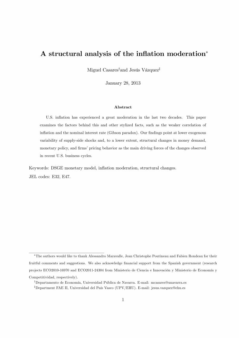
Since 1995, there has been a great moderation of U.S. inflation, characterized by a low average

rate and mild fluctuations around it (see Figure 1). This is particular striking when compared to

high average inflation and strong volatility observed in the three decades before 1995. The inflation

moderation might be connected to changes in other economic variables. Indeed, the Fed funds rate

also displays low levels and low variability after 1995. The decline in volatility is also found in the

rate of growth of some monetary aggregates.1

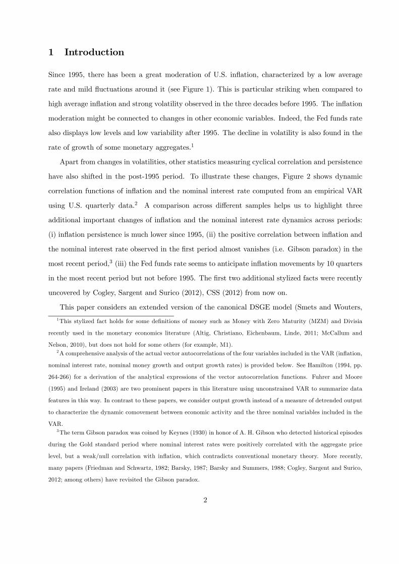
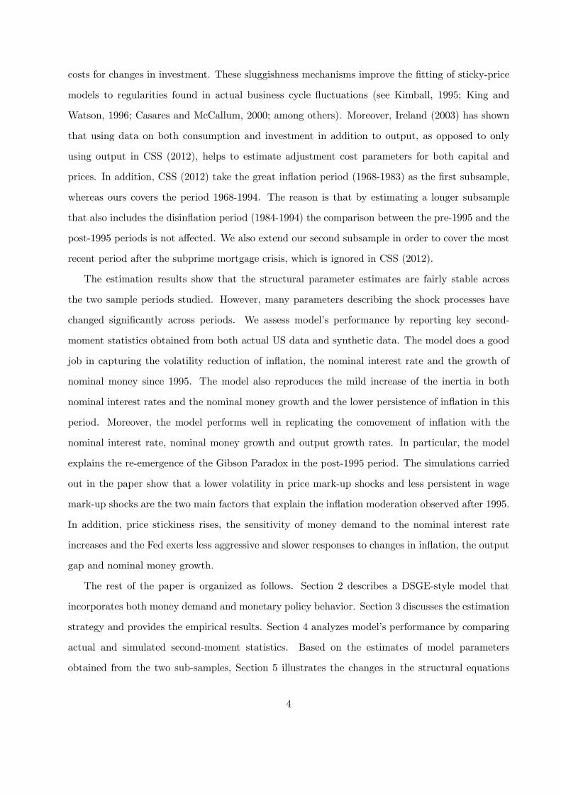
Apart from changes in volatilities, other statistics measuring cyclical correlation and persistence

have also shifted in the post-1995 period. To illustrate these changes, Figure 2 shows dynamic

correlation functions of inflation and the nominal interest rate computed from an empirical VAR

using U.S. quarterly data.2 A comparison across different samples helps us to highlight three

additional important changes of inflation and the nominal interest rate dynamics across periods:

(i) inflation persistence is much lower since 1995, (ii) the positive correlation between inflation and

the nominal interest rate observed in the first period almost vanishes (i.e. Gibson paradox) in the

most recent period,3 (iii) the Fed funds rate seems to anticipate inflation movements by 10 quarters

in the most recent period but not before 1995. The first two additional stylized facts were recently

uncovered by Cogley, Sargent and Surico (2012), CSS (2012) from now on.

This paper considers an extended version of the canonical DSGE model (Smets and Wouters,

1This stylized fact holds for some definitions of money such as Money with Zero Maturity (MZM) and Divisia

recently used in the monetary economics literature (Altig, Christiano, Eichenbaum, Linde, 2011; McCallum and

Nelson, 2010), but does not hold for some others (for example, M1).2A comprehensive analysis of the actual vector autocorrelations of the four variables included in the VAR (inflation,

nominal interest rate, nominal money growth and output growth rates) is provided below. See Hamilton (1994, pp.

264-266) for a derivation of the analytical expressions of the vector autocorrelation functions. Fuhrer and Moore

(1995) and Ireland (2003) are two prominent papers in this literature using unconstrained VAR to summarize data

features in this way. In contrast to these papers, we consider output growth instead of a measure of detrended output

to characterize the dynamic comovement between economic activity and the three nominal variables included in the

VAR.3The term Gibson paradox was coined by Keynes (1930) in honor of A. H. Gibson who detected historical episodes

during the Gold standard period where nominal interest rates were positively correlated with the aggregate price

level, but a weak/null correlation with inflation, which contradicts conventional monetary theory. More recently,

many papers (Friedman and Schwartz, 1982; Barsky, 1987; Barsky and Summers, 1988; Cogley, Sargent and Surico,

2012; among others) have revisited the Gibson paradox.

2

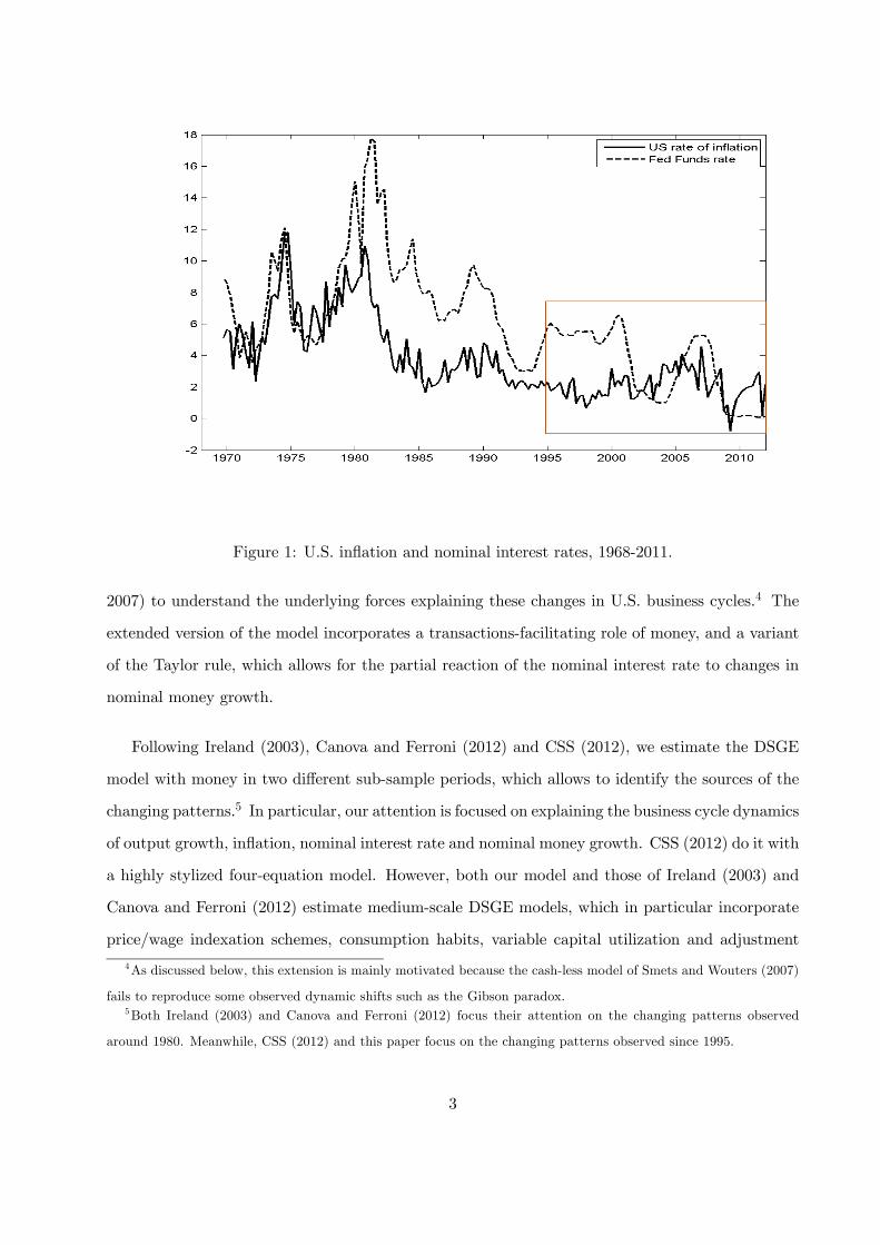
Figure 1: U.S. inflation and nominal interest rates, 1968-2011.

2007) to understand the underlying forces explaining these changes in U.S. business cycles.4 The

extended version of the model incorporates a transactions-facilitating role of money, and a variant

of the Taylor rule, which allows for the partial reaction of the nominal interest rate to changes in

nominal money growth.

Following Ireland (2003), Canova and Ferroni (2012) and CSS (2012), we estimate the DSGE

model with money in two different sub-sample periods, which allows to identify the sources of the

changing patterns.5 In particular, our attention is focused on explaining the business cycle dynamics

of output growth, inflation, nominal interest rate and nominal money growth. CSS (2012) do it with

a highly stylized four-equation model. However, both our model and those of Ireland (2003) and

Canova and Ferroni (2012) estimate medium-scale DSGE models, which in particular incorporate

price/wage indexation schemes, consumption habits, variable capital utilization and adjustment

4As discussed below, this extension is mainly motivated because the cash-less model of Smets and Wouters (2007)

fails to reproduce some observed dynamic shifts such as the Gibson paradox.5Both Ireland (2003) and Canova and Ferroni (2012) focus their attention on the changing patterns observed

around 1980. Meanwhile, CSS (2012) and this paper focus on the changing patterns observed since 1995.

3

costs for changes in investment. These sluggishness mechanisms improve the fitting of sticky-price

models to regularities found in actual business cycle fluctuations (see Kimball, 1995; King and

Watson, 1996; Casares and McCallum, 2000; among others). Moreover, Ireland (2003) has shown

that using data on both consumption and investment in addition to output, as opposed to only

using output in CSS (2012), helps to estimate adjustment cost parameters for both capital and

prices. In addition, CSS (2012) take the great inflation period (1968-1983) as the first subsample,

whereas ours covers the period 1968-1994. The reason is that by estimating a longer subsample

that also includes the disinflation period (1984-1994) the comparison between the pre-1995 and the

post-1995 periods is not affected. We also extend our second subsample in order to cover the most

recent period after the subprime mortgage crisis, which is ignored in CSS (2012).

The estimation results show that the structural parameter estimates are fairly stable across

the two sample periods studied. However, many parameters describing the shock processes have

changed significantly across periods. We assess model’s performance by reporting key second-

moment statistics obtained from both actual US data and synthetic data. The model does a good

job in capturing the volatility reduction of inflation, the nominal interest rate and the growth of

nominal money since 1995. The model also reproduces the mild increase of the inertia in both

nominal interest rates and the nominal money growth and the lower persistence of inflation in this

period. Moreover, the model performs well in replicating the comovement of inflation with the

nominal interest rate, nominal money growth and output growth rates. In particular, the model

explains the re-emergence of the Gibson Paradox in the post-1995 period. The simulations carried

out in the paper show that a lower volatility in price mark-up shocks and less persistent in wage

mark-up shocks are the two main factors that explain the inflation moderation observed after 1995.

In addition, price stickiness rises, the sensitivity of money demand to the nominal interest rate

increases and the Fed exerts less aggressive and slower responses to changes in inflation, the output

gap and nominal money growth.

The rest of the paper is organized as follows. Section 2 describes a DSGE-style model that

incorporates both money demand and monetary policy behavior. Section 3 discusses the estimation

strategy and provides the empirical results. Section 4 analyzes model’s performance by comparing

actual and simulated second-moment statistics. Based on the estimates of model parameters

obtained from the two sub-samples, Section 5 illustrates the changes in the structural equations

4

Figure 2: Vector autocorrelation and cross-correlation functions from US inflation and nominal

interest rates.

from 1995 onwards. In addition, this section runs a large set of counterfactual exercises to assess the

relative importance of key model elements to explain the swing of business cycle patterns. Finally,

Section 6 concludes.

2 A DSGE model with money

This paper considers a modified version of the Smets and Wouters (2007) model to introduce money.

The role of money is defined by its specific function: being the medium-of-exchange to carry out

transactions. Thus, a transactions technology is presented where the stock of real money can be

used to save transaction costs.6 Any increase in real money holdings has a negative impact on

transactions costs, with decreasing marginal returns. Meanwhile, money is supplied by the central

6The introduction of money through a transaction cost technology instead of a money-in-the-utility function

specification used by Ireland (2003) and Canova and Ferroni (2012) is empirically motivated. The former approach

is somewhat more flexible than the latter to accommodate the observed dynamic shifts.

5

bank to support the implementation of a Taylor (1993)-style stabilizing monetary policy rule.

Households maximize intertemporal utility that is non-separable between consumption and

labor as in Smets and Wouters (2007). There is also a external consumption habit component and

a consumption preference shock. Meanwhile, the budget constraint incorporates (real) spending

on transaction costs, and the possibility of using savings for a net increase in real money balances.

Based on the monetary model of Casares (2007), let us consider the following transactions

technology for a j representative household

Ht(j) = a0 + a1Ct (j)

⎛⎝ Ct (j)

exp (εχt )³Mt(j)Pt− λm

Mt−1Pt−1

´⎞⎠

a21−a2

, (1)

where Ht(j) is the amount of real income required to cover the transaction costs of a household

that consumes Ct(j) and holds the amount of real moneyMt(j)Pt

. The parameters of the transactions

technology function satisfy a0, a1 > 0, 0 < a2 < 1, 0 < λm < 1, while εχt is a money-augmenting

AR(1) shock.7 As a distinctive characteristic from Casares (2007), there is (external) monetary

habits that measure endogenous inertia on the demand for real money. The first-order conditions

bring about the money demand equation

−HMt(j)Pt

=Rt

1 +Rt, (2)

that equates the marginal return of monetary services, −HMt(j)Pt

, to the discounted value of the

nominal interest rate, Rt1+Rt

, as the marginal (opportunity) cost of money holdings. The fluctuations

of the marginal service of transactions-facilitating money can be taken from the partial derivative

of (1) and substituted in the optimality condition (2) to yield the semi-log real money demand

equation

mt = (λm/γ)mt−1 + (1− λm/γ) ct − (1−λm/γ)(1−a2)Rss Rt − a2 (1− λm/γ) ε

χt , (3)

where mt and ct denote respectively log fluctuations of real money and consumption with respect

to their steady-state levels, γ is the steady state output growth and Rss is the steady-state nominal

interest rate. The algebra involved is shown in the appendix.

7As shown in the Appendix, the partial derivatives of the transaction costs function imply the desirable properties:

HCt(j)

> 0, HCt(j)Ct(j)

> 0, HMt(j)Pt

< 0, HMt(j)Pt

Mt(j)Pt

> 0 and HCt(j)

Mt(j)Pt

< 0.

6

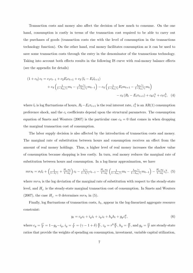
Transaction costs and money also affect the decision of how much to consume. On the one

hand, consumption is costly in terms of the transaction cost required to be able to carry out

the purchases of goods (transaction costs rise with the level of consumption in the transactions

technology function). On the other hand, real money facilitates consumption as it can be used to

save some transaction costs through the entry in the denominator of the transactions technology.

Taking into account both effects results in the following IS curve with real-money balance effects

(see the appendix for details)

(1 + c4) ct = c1ct−1 + c2Etct+1 + c3 (lt −Etlt+1)

+ c4

³1

1−λm/γmt − λm/γ1−λm/γmt−1

´− c4

³1

1−λm/γEtmt+1 − λm/γ1−λm/γmt

´− c5 (Rt −Etπt+1) + c6ε

χt + c7ε

bt , (4)

where lt is log fluctuations of hours, Rt−Etπt+1 is the real interest rate, εbt is an AR(1) consumption

preference shock, and the ci coefficients depend upon the structural parameters. The consumption

equation of Smets and Wouters (2007) is the particular case c4 = 0 that comes in when dropping

the marginal transaction cost of consumption.

The labor supply decision is also affected by the introduction of transaction costs and money.

The marginal rate of substitution between hours and consumption receives an effect from the

amount of real money holdings. Thus, a higher level of real money increases the shadow value

of consumption because shopping is less costly. In turn, real money reduces the marginal rate of

substitution between hours and consumption. In a log-linear approximation, we have

mrst = σllt +³

11−λ/γ +

HC a21−a2

´ct − λ/γ

1−λ/γ ct−1 −HC a21−a2

³1

1−λm/γmt − λm/γ1−λm/γmt−1

´− HC a2

1−a2 εχt , (5)

where mrst is the log deviation of the marginal rate of substitution with respect to the steady-state

level, and HC is the steady-state marginal transaction cost of consumption. In Smets and Wouters

(2007), the case HC = 0 determines mrst in (5).

Finally, log fluctuations of transaction costs, ht, appear in the log-linearized aggregate resource

constraint:

yt = cyct + iyit + zyzt + hyht + gyεgt , (6)

where cy = CY = 1−gy−iy, iy = I

Y = (γ − 1 + δ) KY , zy = rk KY , hy =HY , and gy =

GY are steady-state

ratios that provide the weights of spending on consumption, investment, variable capital utilization,

7

transaction costs, and exogenous spending. As in Smets and Wouters (2007), the component of

exogenous spending εgt is determined by an AR(1) process correlated with productivity innovations

to collect possible fiscal or net exports shocks. The value of ht is provided by the loglinearized

transactions technology function

ht =1−(a0/H)1−a2

³ct − a2

³1

1−λm/γmt − λm/γ1−λm/γmt−1

´− a2ε

χt

´. (7)

Regarding the central-bank behavior, systematic monetary policy actions are governed by a

Taylor (1983)-type rule extended with a stabilizing response to changes in the growth of nominal

money, μt = logMt−logMt−1. In addition, there is a smoothing component, 0 < ρ < 1, that brings

a partial adjustment between the previous nominal interest rate and the Taylor-style targeting as

follows:8

Rt = ρRt−1 + (1− ρ)[rππt + ry(yt − ypt ) + rμμt] + εRt , (8)

where yt and ypt denote output and potential output, respectively; and εRt is a random disturbance

following an AR(1) process with persistence parameter denoted by ρR and the standard deviation

of the innovations of the AR(1) process denoted by σR.

The complete set of loglinearized dynamic equations of the DSGE monetary model and the set

of structural parameters are available in the appendix.

3 Estimation results

The DSGE model with money has been estimated for two sub-samples of quarterly U.S. data,

1968:1 to 1994:4 and 1995:1 to 2011:3, taking the first quarter of 1995 as the starting period of the

great moderation of inflation with low average rates and little variability. The choice of the sample

split can be found by both simple inspection of the U.S. inflation time series plot (see Figure 1)

and the changes in persistence and correlation patterns of inflation and the nominal interest rate8We have experimented with additional formulations for the policy rule, included the hybrid policy rule considered

by Ireland (2003), where the central bank monitors monetary policy by adjusting a linear combination of the nominal

interest rate and the money growth rate in response to output gap and inflation movements from their steady-state

values. The qualitative results of the paper are robust to all policy specifications considered. The rationale for this

empirical finding is simple: equation (8) can be viewed as an observational equivalent reduced-form of a wide range

of alternative monetary rules where either the nominal interest rate or the nominal money growth is the instrument

monitored by the central bank. Of course, the interpretation of the monetary policy shock changes accordingly.

8

shown in Figure 2. Interestingly, a more sophisticated method suggested in CSS (2012), based on

a VAR with drifting coefficients and stochastic volatility, points out 1995 as the year when the

Gibson paradox re-emerged and inflation persistence fell.

As a monetary model, one of the observable variables is the log difference of "Money with Zero

Maturity" (MZM) calculated by the Federal Reserve Bank of St. Louis.9 The rest of the observables

corresponds to the list used in Smets and Wouters (2007): the inflation rate, the Federal funds rate,

the log of hours worked and the log differences of the real GDP, real consumption, real investment

and the real wage.

The estimation follows a two-step Bayesian procedure. In the first step, the log posterior

function is maximized in a way that combines the prior information of the parameters with the

empirical likelihood of the data. In a second step, we perform the Metropolis-Hastings algorithm

to compute the posterior distribution of the parameter set.10

In terms of the priors, we select the same set of distributions as in Smets and Wouters

(2007), which are shown in the first three columns of Tables 1A and 1B and where we have

also borrowed their notation for the structural parameters. The introduction of transactions-

facilitating money brings about a few additional parameters. The prior distribution of λm, the

parameter that measures monetary habits, is identical to the one associated with consumption

habits, λ, with the exception of the standard deviation, which is twice larger for λm reflecting

our rather diffuse prior knowledge of this parameter. The prior distribution of the elasticity

parameter in the transaction costs technology, a2, is described by a beta distribution with

mean 0.5 and standard deviation 0.2. The prior distribution of the policy parameter rμ

is a normal distribution with mean 0.5 and standard deviation 0.2. Finally, the prior

9As discussed in McCallum and Nelson (2010) and Altig, Christiano, Eichenbaum and Linde (2011), there are

hybrid definitions of money such as MZM or Divisia more adequate for providing a representation of the medium-

of-exchange role of money than more conventional aggregates such as the Monetary Base, M1 or M2. Moreover, the

choice of MZM is empirically motivated from the analysis of the overall performance of alternative specifications of the

medium-scale model in replicating the stylized facts described in the Introduction. These alternative specifications

include money-in-the-utility function, alternative specifications of the policy rule and alternative definitions of money.10All estimation exercises are performed with DYNARE free routine software, which can be downloaded from

http://www.dynare.org. A sample of 250,000 draws was used (ignoring the first 20% of draws). A step size of

0.30 resulted in an average acceptation rate of roughly 31% (27%) in the estimation procedure of the first (second)

sub-sample period.

9

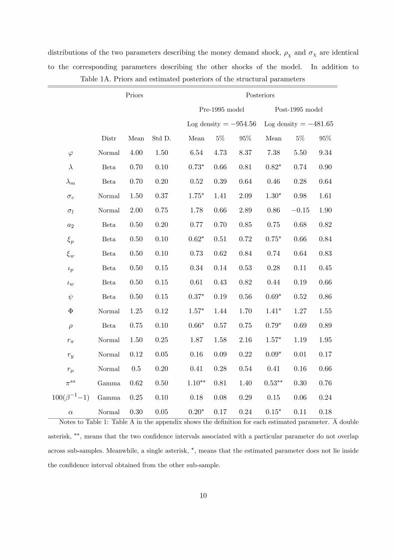
distributions of the two parameters describing the money demand shock, ρχ and σχ are identical

to the corresponding parameters describing the other shocks of the model. In addition to

Table 1A. Priors and estimated posteriors of the structural parameters

Priors Posteriors

Pre-1995 model Post-1995 model

Log density = −954.56 Log density = −481.65Distr Mean Std D. Mean 5% 95% Mean 5% 95%

ϕ Normal 4.00 1.50 6.54 4.73 8.37 7.38 5.50 9.34

λ Beta 0.70 0.10 0.73∗ 0.66 0.81 0.82∗ 0.74 0.90

λm Beta 0.70 0.20 0.52 0.39 0.64 0.46 0.28 0.64

σc Normal 1.50 0.37 1.75∗ 1.41 2.09 1.30∗ 0.98 1.61

σl Normal 2.00 0.75 1.78 0.66 2.89 0.86 −0.15 1.90

a2 Beta 0.50 0.20 0.77 0.70 0.85 0.75 0.68 0.82

ξp Beta 0.50 0.10 0.62∗ 0.51 0.72 0.75∗ 0.66 0.84

ξw Beta 0.50 0.10 0.73 0.62 0.84 0.74 0.64 0.83

ιp Beta 0.50 0.15 0.34 0.14 0.53 0.28 0.11 0.45

ιw Beta 0.50 0.15 0.61 0.43 0.82 0.44 0.19 0.66

ψ Beta 0.50 0.15 0.37∗ 0.19 0.56 0.69∗ 0.52 0.86

Φ Normal 1.25 0.12 1.57∗ 1.44 1.70 1.41∗ 1.27 1.55

ρ Beta 0.75 0.10 0.66∗ 0.57 0.75 0.79∗ 0.69 0.89

rπ Normal 1.50 0.25 1.87 1.58 2.16 1.57∗ 1.19 1.95

ry Normal 0.12 0.05 0.16 0.09 0.22 0.09∗ 0.01 0.17

rμ Normal 0.5 0.20 0.41 0.28 0.54 0.41 0.16 0.66

πss Gamma 0.62 0.50 1.10∗∗ 0.81 1.40 0.53∗∗ 0.30 0.76

100(β−1−1) Gamma 0.25 0.10 0.18 0.08 0.29 0.15 0.06 0.24

α Normal 0.30 0.05 0.20∗ 0.17 0.24 0.15∗ 0.11 0.18

Notes to Table 1: Table A in the appendix shows the definition for each estimated parameter. A double

asterisk, ∗∗, means that the two confidence intervals associated with a particular parameter do not overlap

across sub-samples. Meanwhile, a single asterisk, ∗, means that the estimated parameter does not lie inside

the confidence interval obtained from the other sub-sample.

10

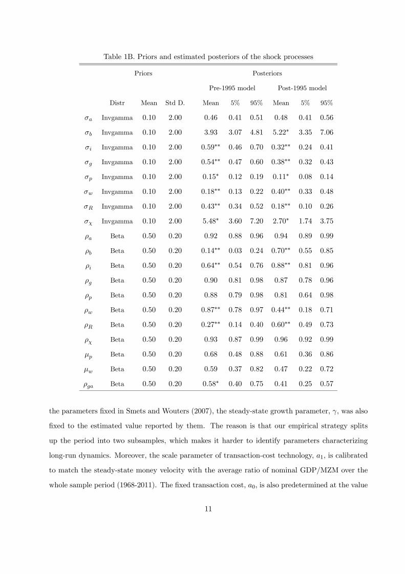
Table 1B. Priors and estimated posteriors of the shock processes

Priors Posteriors

Pre-1995 model Post-1995 model

Distr Mean Std D. Mean 5% 95% Mean 5% 95%

σa Invgamma 0.10 2.00 0.46 0.41 0.51 0.48 0.41 0.56

σb Invgamma 0.10 2.00 3.93 3.07 4.81 5.22∗ 3.35 7.06

σi Invgamma 0.10 2.00 0.59∗∗ 0.46 0.70 0.32∗∗ 0.24 0.41

σg Invgamma 0.10 2.00 0.54∗∗ 0.47 0.60 0.38∗∗ 0.32 0.43

σp Invgamma 0.10 2.00 0.15∗ 0.12 0.19 0.11∗ 0.08 0.14

σw Invgamma 0.10 2.00 0.18∗∗ 0.13 0.22 0.40∗∗ 0.33 0.48

σR Invgamma 0.10 2.00 0.43∗∗ 0.34 0.52 0.18∗∗ 0.10 0.26

σχ Invgamma 0.10 2.00 5.48∗ 3.60 7.20 2.70∗ 1.74 3.75

ρa Beta 0.50 0.20 0.92 0.88 0.96 0.94 0.89 0.99

ρb Beta 0.50 0.20 0.14∗∗ 0.03 0.24 0.70∗∗ 0.55 0.85

ρi Beta 0.50 0.20 0.64∗∗ 0.54 0.76 0.88∗∗ 0.81 0.96

ρg Beta 0.50 0.20 0.90 0.81 0.98 0.87 0.78 0.96

ρp Beta 0.50 0.20 0.88 0.79 0.98 0.81 0.64 0.98

ρw Beta 0.50 0.20 0.87∗∗ 0.78 0.97 0.44∗∗ 0.18 0.71

ρR Beta 0.50 0.20 0.27∗∗ 0.14 0.40 0.60∗∗ 0.49 0.73

ρχ Beta 0.50 0.20 0.93 0.87 0.99 0.96 0.92 0.99

μp Beta 0.50 0.20 0.68 0.48 0.88 0.61 0.36 0.86

μw Beta 0.50 0.20 0.59 0.37 0.82 0.47 0.22 0.72

ρga Beta 0.50 0.20 0.58∗ 0.40 0.75 0.41 0.25 0.57

the parameters fixed in Smets and Wouters (2007), the steady-state growth parameter, γ, was also

fixed to the estimated value reported by them. The reason is that our empirical strategy splits

up the period into two subsamples, which makes it harder to identify parameters characterizing

long-run dynamics. Moreover, the scale parameter of transaction-cost technology, a1, is calibrated

to match the steady-state money velocity with the average ratio of nominal GDP/MZM over the

whole sample period (1968-2011). The fixed transaction cost, a0, is also predetermined at the value

11

that implies that the ratio of total transaction costs over consumption is equal to 0.01 in steady

state.

Table 1 shows the estimation results by reporting the posterior mean values together with

the 5% and 95% quantiles of the posterior distribution for the two sub-samples studied. Many

of the estimates look rather stable across sub-samples. In particular, indexation parameters are

rather similar in the two sub-samples whereas policy parameters ρ and rπ have only changed

marginally. However, there are several noticeable differences. Thus, the consumption habit

formation parameter, λ, and the price rigidity probability parameter, ξp, are higher in the after-

1995 subsample. Meanwhile, the steady-state rate of inflation, πss, is much lower. Moreover,

many of the estimates of shock processes change significantly across sub-samples. Thus, the

persistence of preference, investment, and monetary policy shocks (ρb, ρi, and ρR) has increased

in the recent period, whereas the opposite occurs for the persistence of wage indexation shocks

(ρw). Furthermore, the standard deviation of the innovations associated with most shocks have

changed across sub-samples. Those corresponding to money demand, monetary policy, investment,

government spending and price indexation shocks are higher in the first sub-sample than in the

second whereas the opposite is true for consumption preference and wage indexation shocks.

4 Model performance

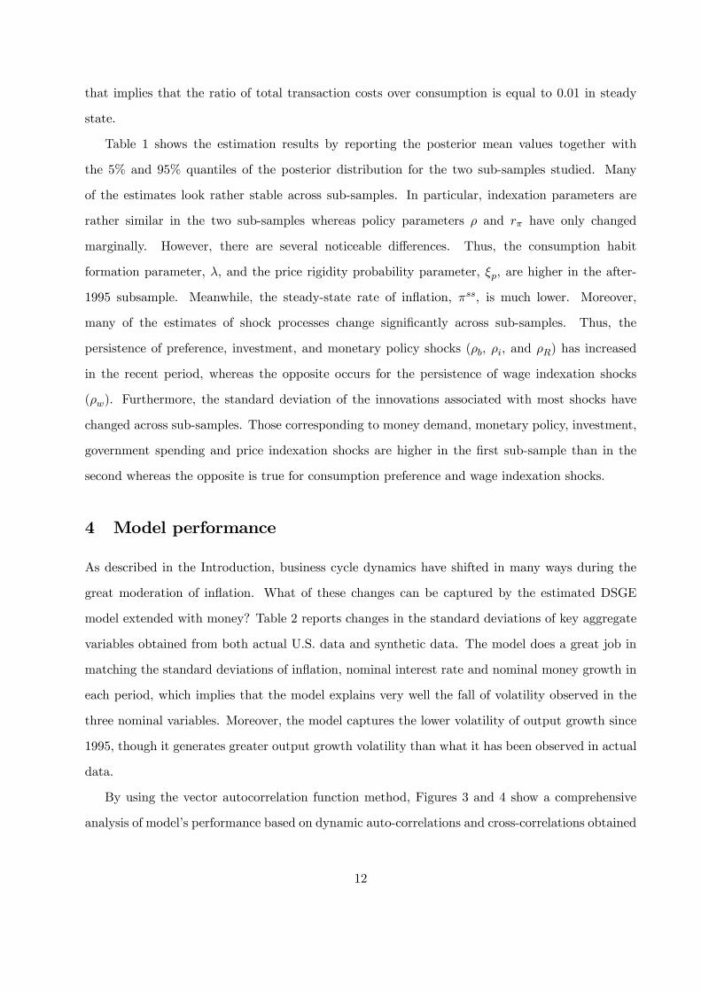
As described in the Introduction, business cycle dynamics have shifted in many ways during the

great moderation of inflation. What of these changes can be captured by the estimated DSGE

model extended with money? Table 2 reports changes in the standard deviations of key aggregate

variables obtained from both actual U.S. data and synthetic data. The model does a great job in

matching the standard deviations of inflation, nominal interest rate and nominal money growth in

each period, which implies that the model explains very well the fall of volatility observed in the

three nominal variables. Moreover, the model captures the lower volatility of output growth since

1995, though it generates greater output growth volatility than what it has been observed in actual

data.

By using the vector autocorrelation function method, Figures 3 and 4 show a comprehensive

analysis of model’s performance based on dynamic auto-correlations and cross-correlations obtained

12

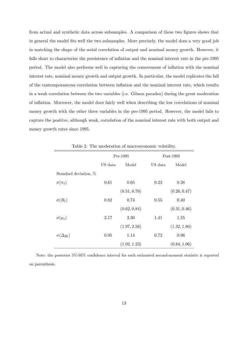
from actual and synthetic data across subsamples. A comparison of these two figures shows that

in general the model fits well the two subsamples. More precisely, the model does a very good job

in matching the shape of the serial correlation of output and nominal money growth. However, it

falls short to characterize the persistence of inflation and the nominal interest rate in the pre-1995

period. The model also performs well in capturing the comovement of inflation with the nominal

interest rate, nominal money growth and output growth. In particular, the model replicates the fall

of the contemporaneous correlation between inflation and the nominal interest rate, which results

in a weak correlation between the two variables (i.e. Gibson paradox) during the great moderation

of inflation. Moreover, the model does fairly well when describing the low correlations of nominal

money growth with the other three variables in the pre-1995 period. However, the model fails to

capture the positive, although weak, correlation of the nominal interest rate with both output and

money growth rates since 1995.

Table 2. The moderation of macroeconomic volatility.

Pre-1995 Post-1995

US data Model US data Model

Standard deviation, %

σ(πt) 0.61 0.65 0.23 0.38

(0.51, 0.76) (0.26, 0.47)

σ(Rt) 0.82 0.74 0.55 0.40

(0.62, 0.84) (0.31, 0.46)

σ(μt) 2.17 2.30 1.41 1.55

(1.97, 2.56) (1.32, 1.80)

σ(∆yt) 0.95 1.14 0.72 0.96

(1.02, 1.23) (0.84, 1.06)

Note: the posterior 5%-95% confidence interval for each estimated second-moment statistic is reported

on parenthesis.

13

Figure 3: Dynamic correlations (1968-1994). US data (*) and estimated model (solid lines with

shaded area showing the 5%-95% confidence interval).

14

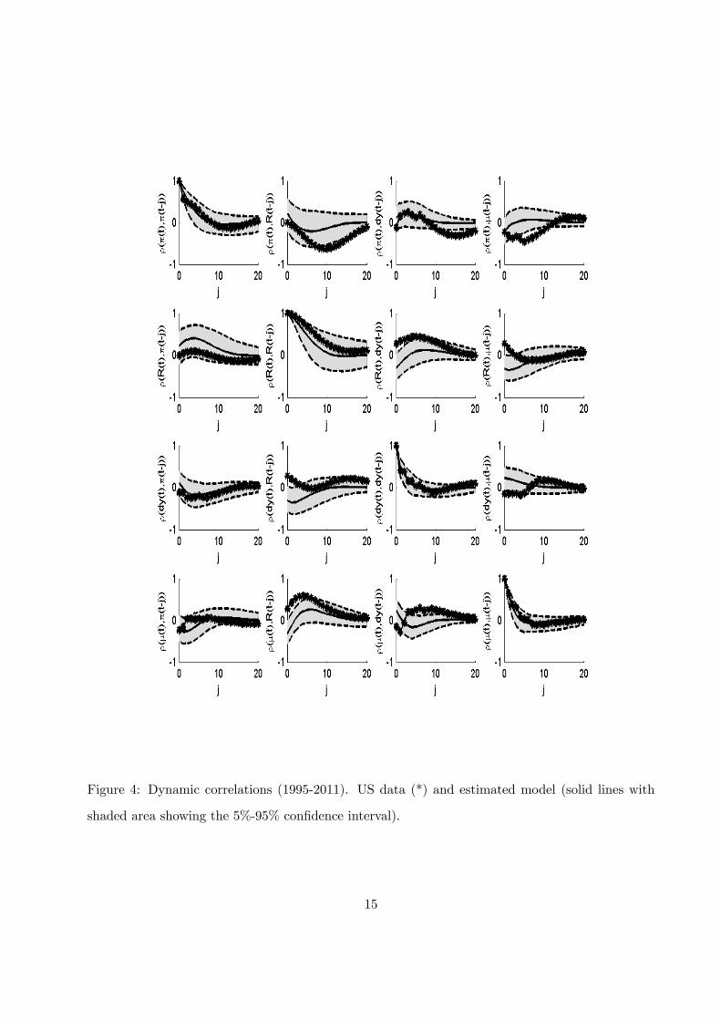
Figure 4: Dynamic correlations (1995-2011). US data (*) and estimated model (solid lines with

shaded area showing the 5%-95% confidence interval).

15

5 What did it change from 1995 onwards?

In this section, we analyze the structural equations and the sources of variability to pin down the

elements that can better illustrate the observed changes that have occurred in recent US business

cycles.

5.1 Inflation dynamics

Price inflation dynamics are governed in the model by the New Keynesian Phillips Curve (NKPC):

πt = π1πt−1 + π2Etπt+1 + π3mct + εpt ,

where π1 =ιp

1+βιp, π2 =

β

1+βιp, and π3 =

11+βιp

∙(1−βξp)(1−ξp)ξp((φp−1)εp+1)

¸and mct denotes the log deviation

of the real marginal cost with respect to the steady-state level. The structural analysis of inflation

dynamics can be illustrated by examining the NKPC across both sub-samples. Hence, the estimates

of the structural parameters give the following NKPC over the first sub-sample (1968:1-1994:4)

πt = 0.25πt−1 + 0.74Etπt+1 + 0.0270mct + εpt ,

εpt = 0.88εpt−1 − 0.68ηpt−1 + ηpt , std(ηp) = 0.15%,

whereas for the second sub-sample (1995:1-2011:4) the estimated NKPC is

πt = 0.22πt−1 + 0.78Etπt+1 + 0.0125mct + εpt ,

εpt = 0.81εpt−1 − 0.61ηpt−1 + ηpt , std(ηp) = 0.11%.

The backward-looking component of inflation is slightly lower after 1995, which indicates that the

endogenous inflation inertia has diminished a bit after 1995. This result is based on the decrease

of nominal inertia described by the price indexation parameter (i.e., ιp falls from 0.34 to 0.28 as

reported in Table 1A). Remarkably, the backward-looking dynamics of price inflation are much

weaker in our estimated NKPC than in the estimation of CSS (2012).

The estimate of the slope coefficient falls substantially in the second period, as it comes down to

less than half of the value found in the first sub-sample. This result is consistent with the increase

in the estimate of the Calvo sticky-price probability. As shown in Table 1, ξp = 0.62 in the period

before 1995, and ξp = 0.75 in the period after 1995. So, the average number of months without

optimal pricing increases from 7.9 months to 12 months. As argued by Smets and Wouters (2007),

16

the price stability period of the Great Moderation (of real variables) may explain the increase in

price stickiness associated with lower menu costs.

As for the exogenous variability of inflation, the comparison of the estimated NKPCs shows

that price mark-up shocks are less volatile and less persistent in the second sub-sample. The

autoregressive coefficient falls by around 8% while the standard deviation of the innovations is 27%

lower.

Summarizing, the decline in inflation volatility after 1995 can be explained by two factors: i)

stickier prices turn inflation less sensitive to real marginal cost fluctuations and ii) firms receive

lower and, more important, less persistent mark-up pricing shocks.11

5.2 Money market

Money demand

The introduction of the transactions-facilitating role of money can shed some light on the possible

influence of variations of money demand behavior to explaining the changes of inflation and interest

rate dynamics. Making the first difference on the money demand equation (3) gives

μt − πt = (λm/γ)¡μt−1 − πt−1

¢+ (1− λm/γ)∆ct − (1−λm/γ)(1−a2)

Rss ∆Rt − a2 (1− λm/γ)∆εχt .

Using the estimates reported in Tables 1A and 1B, the pre-1995 subsample is characterized by the

following money demand behavior

μt − πt = 0.52¡μt−1 − πt−1

¢+ 0.48∆ct − 8.63∆Rt − 0.37∆εχt ,

εχt = 0.93εχt−1 + ηχt , std(ηχ) = 5.48%,

whereas in the post-1995 subsample

μt − πt = 0.46¡μt−1 − πt−1

¢+ 0.54∆ct − 19.85∆Rt − 0.41∆εχt ,

εχt = 0.96εχt−1 + ηχt , std(ηχ) = 2.70%.

It is quite noticeable from the comparison that the semi-elasticity of real money with respect to the

nominal interest rate has increased dramatically in the second period. Both the decline of monetary

11The qualification "more important", associated with less persistent mark-up shocks, made in this sentence is

rather relevant because intertemporal rational agents decisions are severely affected by persistent shocks.

17

habits λm and the deep fall of (inflation and) the nominal interest rate in the steady state, Rss, are

the two model elements behind this change. The resulting dynamics of money demand imply that in

equilibrium nominal interest rates are quite insensitive to changes in either consumption, inflation,

nominal money growth or exogenous perturbations. For example, after a mark-up shock that raises

inflation, the required increase in the nominal interest to adjust down real money demand would be

quantitatively much smaller. Hence, the increase in interest-rate semi-elasticity of money demand

can serve to explain both the low volatility of the nominal interest rate and the reduction in its

cyclical correlation with inflation, observed after 1995.

Money supply (monetary policy)

Regarding money supply behavior, the Taylor-style rule (8) incorporates responses of the nominal

interest rate to nominal money growth as part of a stabilizing systematic monetary policy. Before

1995, the estimated monetary policy rule is

Rt = 0.66Rt−1 + 0.64πt + 0.05(yt − ypt ) + 0.14μt + εRt ,

εRt = 0.27εRt−1 + ηRt , std(ηR) = 0.43%.

Meanwhile, in the second sub-sample that begins in 1995 the estimated monetary policy is

Rt = 0.79Rt−1 + 0.33πt + 0.02(yt − ypt ) + 0.09μt + εRt ,

εRt = 0.60εRt−1 + ηRt , std(ηR) = 0.18%.

The comparison highlights some relevant changes. First, the nominal interest rate adjusts more

gradually during the period of the great inflation moderation, as the smoothing (inertia) coefficient

increases from 0.66 to 0.79. Second, the response coefficients to inflation, the output gap, and

money growth are lower after 1995, which might somewhat reflect a sense of a loose central-bank

policy during the period of inflation moderation. In other words, monetary policy becomes more

discretional and less rule-oriented, as the systematic behavior weakens.12 By contrast, CSS (2012)

find a more anti-inflationary monetary-policy rule as one of the factors behind the return of the

Gibson paradox. These different results might be partially explained by the different sample periods

used in the two papers.13

12Contributing to this line of argument, Taylor (2012) claims that, from 2003, Fed’s monetary policy deviated

significantly from a Taylor (1983)-type rule to become quite discretional.13 In particular, our paper considers observations after 2007, ignored by CSS (2012), which capture the rather loose

18

5.3 Real wage dynamics

Wage setting behavior and nominal rigidities à la Calvo (1983) lead to the following expression for

the dynamic evolution of real wages

wt = w1wt−1 + (1− w1) (Etwt+1 +Etπt+1)− w2πt + w3πt−1 − w4 (wt −mrst) + εwt ,

where w1 = 11+β

, w2 =1+βιw1+β

, w3 = ιw1+β

, and w4 =11+β

∙(1−βξw)(1−ξw)ξw((φw−1)εw+1)

¸. In the estimation, the

curvature of the Kimball labor aggregator is fixed at εw = 10.0 and the steady-state wage mark-up

is φw = 1.5, following Smets and Wouters (2007). The wage mark-up, wt −mrst, measured as the

log difference between the real wage and the marginal rate of substitution between working and

consuming is the key determinant of real wage fluctuations. The estimates before 1995 imply

wt = 0.50wt−1 + 0.50 (Etwt+1 +Etπt+1)− 0.80πt + 0.30πt−1 − 0.0094 (wt −mrst) + εwt ,

εwt = 0.87εwt−1 − 0.59ηwt−1 + ηwt , std(ηw) = 0.18%.

Meanwhile, in the sample after 1995 the estimated real wage equation is

wt = 0.50wt−1 + 0.50 (Etwt+1 +Etπt+1)− 0.72πt + 0.22πt−1 − 0.0079 (wt −mrst) + εwt ,

εwt = 0.44εwt−1 − 0.47ηwt−1 + ηwt , std(ηw) = 0.40%.

The structural components of real wage dynamics (backward/forward looking coefficients, slope

coefficient) show slight shifts after 1995. The estimates of wage-stickiness, ξw, barely change across

samples, while wage indexation on lagged inflation, ιw, falls in the second subsample (see Table

2 for the numbers). Nevertheless, significant differences are observed in the exogenous process

that collects wage mark-up shocks. The coefficient of autocorrelation falls from 0.87 to 0.44. The

moving-average coefficient is also lower, while the innovations have a higher standard deviation

after 1995. The sizable reduction of persistence in wage mark-up shocks has dramatic effects on

the sources of business cycle variability after 1995, as documented next.

5.4 Sources of variability

Both the impulse-response functions and the variance decomposition provide model-based

information about how the exogenous sources of variability shape the business cycle fluctuations.

monetary policy implemented by the Fed since the subprime mortgage crisis.

19

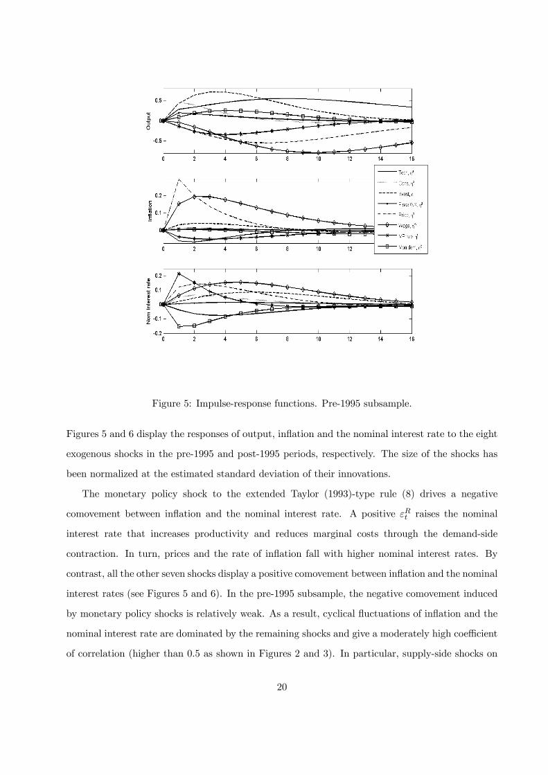
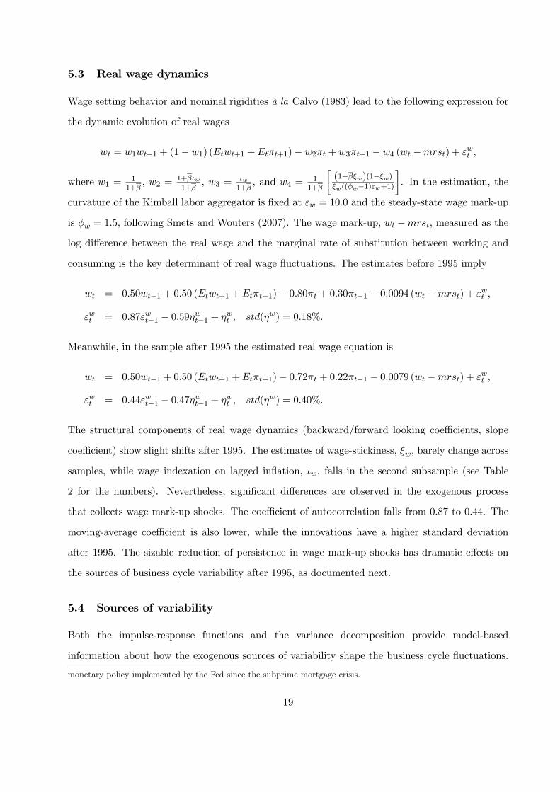
Figure 5: Impulse-response functions. Pre-1995 subsample.

Figures 5 and 6 display the responses of output, inflation and the nominal interest rate to the eight

exogenous shocks in the pre-1995 and post-1995 periods, respectively. The size of the shocks has

been normalized at the estimated standard deviation of their innovations.

The monetary policy shock to the extended Taylor (1993)-type rule (8) drives a negative

comovement between inflation and the nominal interest rate. A positive εRt raises the nominal

interest rate that increases productivity and reduces marginal costs through the demand-side

contraction. In turn, prices and the rate of inflation fall with higher nominal interest rates. By

contrast, all the other seven shocks display a positive comovement between inflation and the nominal

interest rates (see Figures 5 and 6). In the pre-1995 subsample, the negative comovement induced

by monetary policy shocks is relatively weak. As a result, cyclical fluctuations of inflation and the

nominal interest rate are dominated by the remaining shocks and give a moderately high coefficient

of correlation (higher than 0.5 as shown in Figures 2 and 3). In particular, supply-side shocks on

20

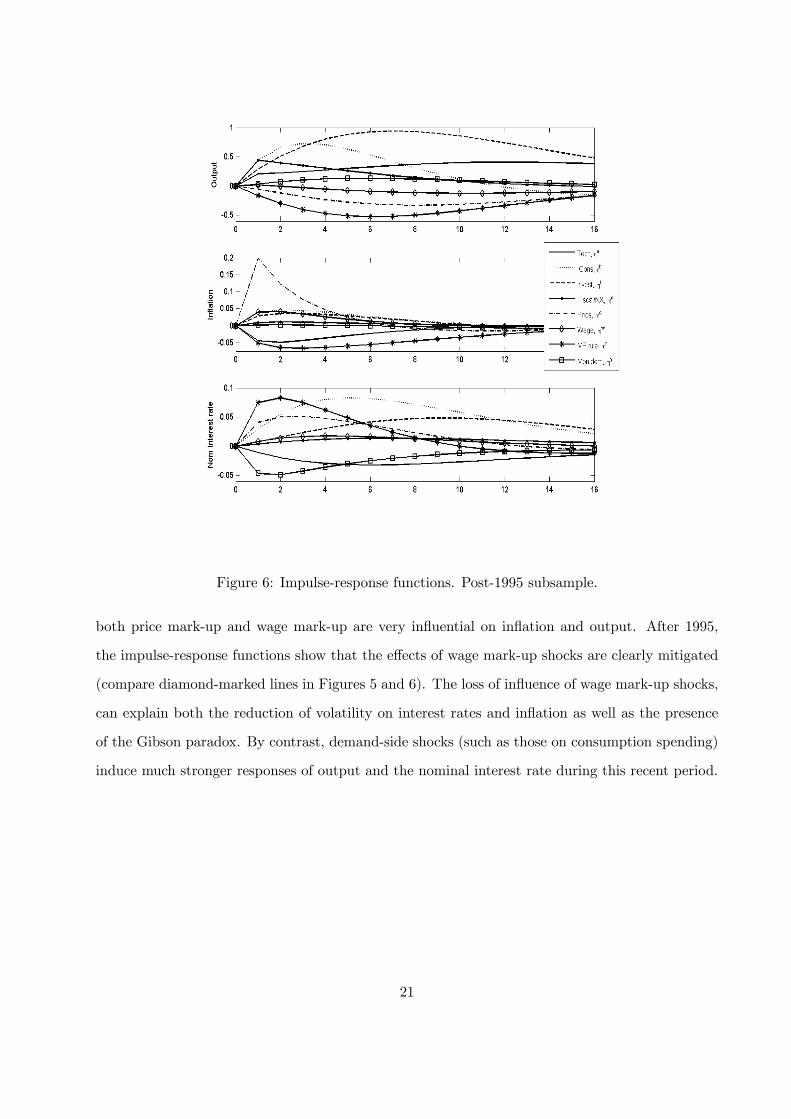
Figure 6: Impulse-response functions. Post-1995 subsample.

both price mark-up and wage mark-up are very influential on inflation and output. After 1995,

the impulse-response functions show that the effects of wage mark-up shocks are clearly mitigated

(compare diamond-marked lines in Figures 5 and 6). The loss of influence of wage mark-up shocks,

can explain both the reduction of volatility on interest rates and inflation as well as the presence

of the Gibson paradox. By contrast, demand-side shocks (such as those on consumption spending)

induce much stronger responses of output and the nominal interest rate during this recent period.

21

Table 3. Variance decomposition, %

Pre-1995 model Post-1995 model

Innovations y ∆y R π μ y ∆y R π μ

Technology, ηa 21.3 8.7 6.5 4.4 2.8 20.2 6.9 7.5 6.8 2.4

Consumption pref., ηb 2.4 18.5 3.2 0.2 0.5 11.6 31.3 36.8 9.1 3.6

Investment, ηi 14.8 21.3 11.2 2.9 2.0 42.0 25.4 19.2 9.1 2.7

Fiscal/Net exports, ηg 5.7 29.8 2.7 0.7 0.6 3.0 20.0 1.3 0.4 0.2

Price-push, ηp 12.9 5.7 15.7 36.6 9.4 8.6 3.8 9.0 46.5 8.4

Wage-push, ηw 37.3 8.8 31.2 49.2 12.5 1.0 0.6 1.6 5.0 1.2

MP rule, ηR 4.0 5.3 15.4 4.3 40.3 12.9 11.4 17.4 21.8 65.8

Money demand, ηχ 1.7 1.8 14.3 1.8 31.9 0.6 0.6 7.2 1.2 15.7

In the variance decomposition of the estimated model (Table 3), the percentages of monetary

policy shocks explaining inflation fluctuations increase in the second sub-sample (from 4% to 22%).

As discussed above, monetary policy shocks increases the negative comovement variability, which

helps explaining the Gibson paradox. However, the most significant change in the sources of

variability is the dramatic decline in the participation of wage-push shocks. As Table 3 reports,

these shocks were responsible for 49.2% of the variability of inflation and 31.2% of the variability

of the nominal interest rate before 1995. The percentages fall below 5% from 1995 onwards. By

contrast, demand-side shocks determine a much greater portion of business cycle fluctuations after

1995 when consumption and investment shocks explain more than 50% of output and the nominal

interest rate variability. Hence, both the estimated variance decomposition and the impulse-

response function analysis indicate a replacement from price/wage mark-up shocks to demand-side

shocks on consumption, investment, and the monetary policy rule as the main sources of variability

in recent US business cycles.

6 Counterfactual experiments

The previous section has discussed the different driving forces explaining the monetary dynamic

changes since 1995. In this section, we carry out a large number of counterfactual experiments in

order to assess the relative importance of these sources. In all these experiments we consider the

22

model parameter estimates obtained from the post-1995 period as the benchmark parameter values

and we recalculate the variance/covariance matrix by considering alternative sets of parameters

values obtained from the pre-1995 estimated model. In doing so, we want to answer the question

of what would happen after 1995 if the values a given group of parameters were the same as the

ones estimated for the pre-1995 sample? Eighteen counterfactual experiments were conducted.

The following are the parameters changing in each of them: (i) rπ, ry, rμ and ρ, which describe

the systematic part of monetary policy, (ii) monetary policy shock parameters (ρR, σR), (iii) all

monetary policy rule parameters (rπ, ry, rμ, ρ, ρR, σR), (iv) money demand technology parameters

(λm, a2, Rss), (v) money demand shock parameters (ρχ, σχ), (vi) all money demand parameters

(λm, a2, Rss, ρχ, σχ), (vii) price setting parameters (ξp, ιp, β), (viii) price mark-up shock parameters

(σp, ρp, μp), (ix) all New Keynesian Phillips curve parameters (ξp, ιp, β, σp, ρp, μp), (x) wage

setting parameters (ξw, ιw, β), (xi) wage mark-up shock parameters (σw, ρw, μw), (xii) all real

wage parameters (ξw, ιw, β, σw, ρw, μw), (xiii) consumption preference parameters (λ, σc), (xiv)

consumption preference shock parameters (ρb, σb), (xv) all consumption parameters (λ, σc, ρb, σb),

(xvi) investment technology parameters (ϕ, ψ), (xvii) investment shock parameters (ρi, σi), and

(xviii) all investment parameters (ϕ, ψ, ρi, σi).

23

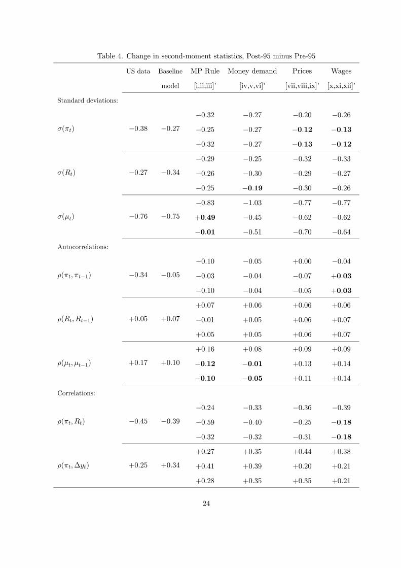
Table 4. Change in second-moment statistics, Post-95 minus Pre-95

US data Baseline MP Rule Money demand Prices Wages

model [i,ii,iii]’ [iv,v,vi]’ [vii,viii,ix]’ [x,xi,xii]’

Standard deviations:

σ(πt) −0.38 −0.27−0.32−0.25−0.32

−0.27−0.27−0.27

−0.20−0.12−0.13

−0.26−0.13−0.12

σ(Rt) −0.27 −0.34−0.29−0.26−0.25

−0.25−0.30−0.19

−0.32−0.29−0.30

−0.33−0.27−0.26

σ(μt) −0.76 −0.75−0.83+0.49

−0.01

−1.03−0.45−0.51

−0.77−0.62−0.70

−0.77−0.62−0.64

Autocorrelations:

ρ(πt, πt−1) −0.34 −0.05−0.10−0.03−0.10

−0.05−0.04−0.04

+0.00

−0.07−0.05

−0.04+0.03

+0.03

ρ(Rt, Rt−1) +0.05 +0.07

+0.07

−0.01+0.05

+0.06

+0.05

+0.05

+0.06

+0.06

+0.06

+0.06

+0.07

+0.07

ρ(μt, μt−1) +0.17 +0.10

+0.16

−0.12−0.10

+0.08

−0.01−0.05

+0.09

+0.13

+0.11

+0.09

+0.14

+0.14

Correlations:

ρ(πt, Rt) −0.45 −0.39−0.24−0.59−0.32

−0.33−0.40−0.32

−0.36−0.25−0.31

−0.39−0.18−0.18

ρ(πt,∆yt) +0.25 +0.34

+0.27

+0.41

+0.28

+0.35

+0.39

+0.35

+0.44

+0.20

+0.35

+0.38

+0.21

+0.21

24

Table 4 shows the change in some selected second-moment statistics between the pre-95 and the

post-95 sub-samples in actual data, in the baseline model and in each counterfactual experiment.14

Bold characters highlight the main sources for these second-moment statistics changes. Results show

that the fall of inflation volatility, σ(πt), is mainly explained by changes in both the parameters

describing wage mark-up shocks (σw, ρw, μw) and price mark-up shocks (σp, ρp, μp). Meanwhile,

the milder fluctuations of the nominal interest rate and the nominal money growth observed in the

most recent period are due to changes in money demand parameters (λm, a2, Rss, ρχ, σχ) and

changes in monetary policy shock parameters (ρR, σR), respectively.

Experiment (xi) suggests that the changes in the wage mark-up shock parameters are partially

responsible for the fall of inflation persistence. Moreover, the changes in monetary policy shock

parameters and money demand parameters help to explain the small increase in nominal money

growth persistence.

Finally, the changes in the wage mark-up shocks largely explain the Gibson paradox and the fall

of both inflation volatility and inflation persistence. These results are in contrast with CSS (2012)

where a more anti-inflationary policy rule and a decline of price indexation are the two sources for

the re-emergence of the Gibson paradox and the fall of inflation persistence. Our counterfactual

experiments show that, with a medium-scale DSGE monetary model, the Gibson paradox, the

fall of inflation persistence and many of the changes observed since 1995 are mostly explained by

exogenous changes in price/wage dynamics: the significant decline in persistence of wage mark-up

shocks and the lower volatility of price mark-up shocks

7 Conclusions

This paper builds a full-fledged estimated DSGE model with money to study the driving forces of

the recent U.S. inflation moderation period and other stylized facts, such as the fall of inflation

persistence and the weakening of inflation and nominal interest rate correlation. Compared to

standard DSGE models, the model incorporates a transaction-facilitating demand for money, a

real-balance effect on consumption, transaction costs as a small percentage of the overall household

14The latest six experiments involving parameters describing consumption and investment demands do not imply

significant changes in second-moments statistics. For the sake of brevity, these experiment results are excluded from

Table 4. They are available from the authors upon request.

25

spending, and a Taylor-type monetary policy rule that reacts to changes in nominal money growth.

Our findings suggest a combination of lower exogenous variability and, to a lower extent,

structural changes in money demand, monetary policy and firms’ pricing behavior as the main

driving forces of the changes observed in the U.S. business cycle since 1995. Regarding the exogenous

variability, the supply-side shocks on both prices and wages, that were dominant in the cyclical

variability in the 70’s and 80’s, loose much of their significance after 1995. Their explanatory power

for business cycle fluctuations has been mostly replaced in the recent period by either investment

spending or interest-rate shocks. The structural analysis of the money market shows that the

estimated interest-rate elasticity of money demand more than doubles in the recent period the

value estimated for the earlier sample period. The lower average rates of return explains this

higher responsiveness of money demand to changes in the nominal interest rates. Other non-

modeled factors could be the greater accessibility of households to a variety of money-like assets,

and the financial innovation of the period. We have also found a swing in monetary policy towards

a more conservative and gradual strategy after 1995. The Fed’s response coefficients to inflation,

the output gap and money growth have been considerably lower after 1995 than what they had

been before. Finally, the estimates of private sector decision making show little differences across

periods. The most remarkable one is that the level of price stickiness rises in the post-95 sample

period. It helps to characterize the observed lower inflation volatility as firms attenuate the reaction

of prices to changes in the marginal costs. This factor and the substantial decline of persistence in

wage-push shocks are key elements explaining the inflation moderation.

26

References

Altig, David, Lawrence J. Christiano, Martin Eichenbaum, and Jesper Linde. 2011. “Firm-

Specific Capital, Nominal Rigidities and the Business Cycle”. Review of Economic Dynamics 14,

225-247.

Barsky Robert B. 1987. “The Fisher Hypothesis and the Forecastability and Persistence of

Inflation”. Journal of Monetary Economics 19, 3-24.

Barsky Robert B., and Lawrence H. Summers. 1988. “Gibson’s Paradox and the Gold

Standard”. Journal of Political Economy 96, 528-550.

Calvo, Guillermo A. 1983. “Staggered Pricing in a Utility-Maximizing Framework.” Journal of

Monetary Economics 12, 383-396.

Canova, Fabio, and Filippo Ferroni (2012). “The Dynamics of US Inflation: Can Monetary

Policy Explain the Changes?” Journal of Econometrics 167, 47-60.

Casares, Miguel. 2007. “The New Keynesian Model and the Euro Area Business Cycle.” Oxford

Bulletin of Economics and Statistics 69, 209-244.

Christiano, Lawrence J., Martin Eichenbaum, and Charles L. Evans. 2005. “Nominal Rigidities

and the Dynamic Effects of a Shock to Monetary Policy.” Journal of Political Economy 113, 1-45.

Cogley, Timothy, Thomas J. Sargent, and Paolo Surico. 2012. “The Return of the Gibson

Paradox.” working paper.

Friedman, Milton, and Anna J. Schwartz. 1982. Monetary Trends in the United States and the

United Kingdom: Their Relation to Income, Prices and Interest Rates, 1867-1975. University of

Chicago Press: Chicago, IL.

Fuhrer, Jeff and George Moore. 1995. “Inflation Persistence.” Quarterly Journal of Economics

440, 127-159.

Hamilton, James D. 1994. Time Series Analysis. Princeton University Press: Princeton, New

Jersey.

Ireland, Peter. 2003. "Endogenous Money or Sticky Prices?" Journal of Monetary Economics

50, 1623-1648.

Keynes, John M. 1930. A Treatise on Money. Mcmillan: London.

Kimball, Miles S. 1995. “The Quantitative Analytics of the Basic Neomonetarist Model.”

Journal of Money, Credit, and Banking, 27: 1241-1277.

27

McCallum, Bennett T., and Edward Nelson. 2010. "Money and inflation: Some critical issues."

Handbook of Monetary Economics, Volume 3, (Chapter 3), pp. 97-153.

Smets, Frank R., and Rafael Wouters. 2007. “Shocks and Frictions in US Business Cycles: A

Bayesian DSGE Approach.” American Economic Review 97, 586-606.

Taylor, John B. 1993. “Discretion Versus Policy Rules in Practice.” Carnegie-Rochester

Conference Series on Public Policy, 39, 195-214.

Taylor, John B. 2012. "Monetary Policy Rules Work and Discretion Doesn’t: A Tale of Two

Eras", Journal of Money Credit and Banking 44, 1017-1032.

28

Appendix

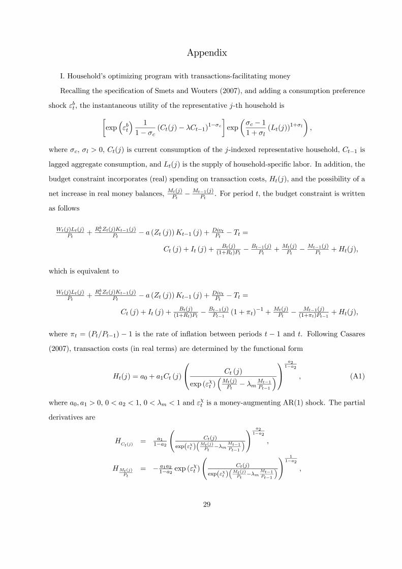
I. Household’s optimizing program with transactions-facilitating money

Recalling the specification of Smets and Wouters (2007), and adding a consumption preference

shock εbt , the instantaneous utility of the representative j-th household is∙exp

³εbt

´ 1

1− σc(Ct(j)− λCt−1)1−σc

¸exp

µσc − 11 + σl

(Lt(j))1+σl

¶,

where σc, σl > 0, Ct(j) is current consumption of the j-indexed representative household, Ct−1 is

lagged aggregate consumption, and Lt(j) is the supply of household-specific labor. In addition, the

budget constraint incorporates (real) spending on transaction costs, Ht(j), and the possibility of a

net increase in real money balances, Mt(j)Pt− Mt−1(j)

Pt. For period t, the budget constraint is written

as follows

Wt(j)Lt(j)Pt

+Rkt Zt(j)Kt−1(j)

Pt− a (Zt (j))Kt−1 (j) + Divt

Pt− Tt =

Ct (j) + It (j) +Bt(j)

(1+Rt)Pt− Bt−1(j)

Pt+ Mt(j)

Pt− Mt−1(j)

Pt+Ht(j),

which is equivalent to

Wt(j)Lt(j)Pt

+Rkt Zt(j)Kt−1(j)

Pt− a (Zt (j))Kt−1 (j) + Divt

Pt− Tt =

Ct (j) + It (j) +Bt(j)

(1+Rt)Pt− Bt−1(j)

Pt−1 (1 + πt)−1 + Mt(j)

Pt− Mt−1(j)(1+πt)Pt−1 +Ht(j),

where πt = (Pt/Pt−1) − 1 is the rate of inflation between periods t − 1 and t. Following Casares

(2007), transaction costs (in real terms) are determined by the functional form

Ht(j) = a0 + a1Ct (j)

⎛⎝ Ct (j)

exp (εχt )³Mt(j)Pt− λm

Mt−1Pt−1

´⎞⎠

a21−a2

, (A1)

where a0, a1 > 0, 0 < a2 < 1, 0 < λm < 1 and εχt is a money-augmenting AR(1) shock. The partial

derivatives are

HCt(j)

= a11−a2

ÃCt(j)

exp(εχt )Mt(j)Pt

−λmMt−1Pt−1

! a21−a2

,

HMt(j)Pt

= − a1a21−a2 exp (ε

χt )

ÃCt(j)

exp(εχt )Mt(j)Pt

−λmMt−1Pt−1

! 11−a2

,

29

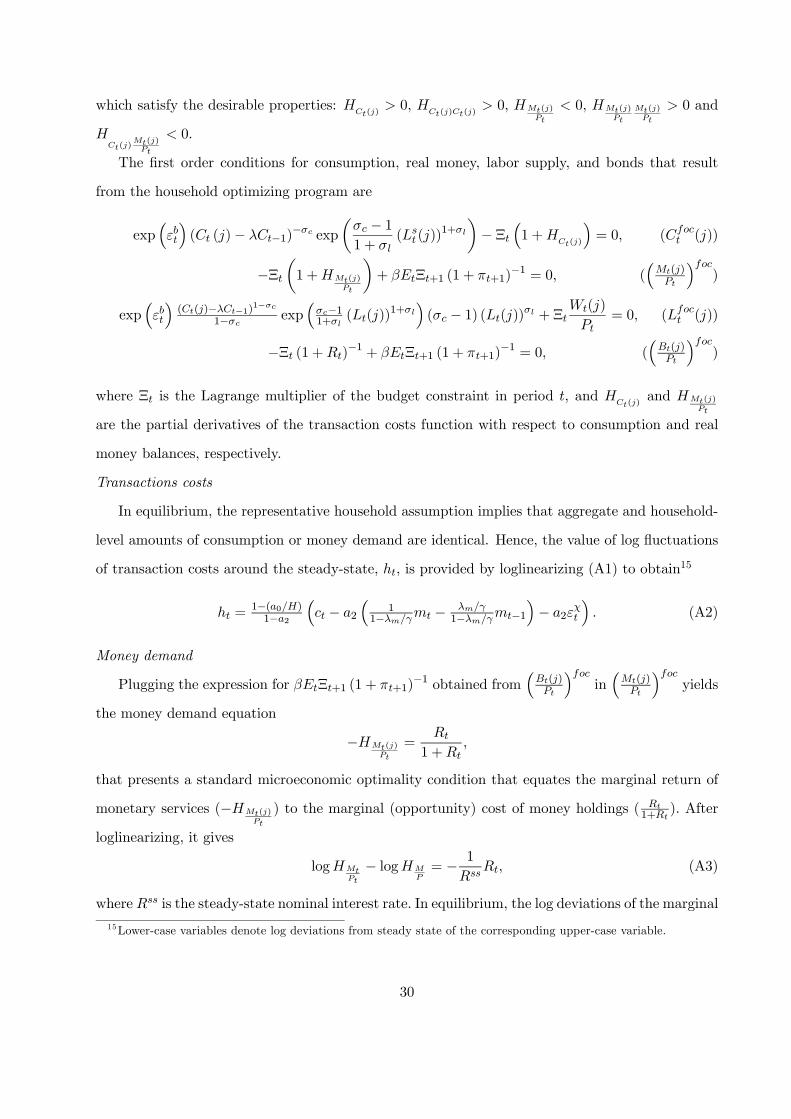
which satisfy the desirable properties: HCt(j)

> 0, HCt(j)Ct(j)

> 0, HMt(j)Pt

< 0, HMt(j)Pt

Mt(j)Pt

> 0 and

HCt(j)

Mt(j)Pt

< 0.

The first order conditions for consumption, real money, labor supply, and bonds that result

from the household optimizing program are

exp³εbt

´(Ct (j)− λCt−1)−σc exp

µσc − 11 + σl

(Lst (j))

1+σl

¶− Ξt

³1 +H

Ct(j)

´= 0, (Cfoc

t (j))

−Ξtµ1 +HMt(j)

Pt

¶+ βEtΞt+1 (1 + πt+1)

−1 = 0, (³Mt(j)Pt

´foc)

exp³εbt

´(Ct(j)−λCt−1)1−σc

1−σc exp³σc−11+σl

(Lt(j))1+σl

´(σc − 1) (Lt(j))

σl + ΞtWt(j)

Pt= 0, (Lfoc

t (j))

−Ξt (1 +Rt)−1 + βEtΞt+1 (1 + πt+1)

−1 = 0, (³Bt(j)Pt

´foc)

where Ξt is the Lagrange multiplier of the budget constraint in period t, and HCt(j)

and HMt(j)Pt

are the partial derivatives of the transaction costs function with respect to consumption and real

money balances, respectively.

Transactions costs

In equilibrium, the representative household assumption implies that aggregate and household-

level amounts of consumption or money demand are identical. Hence, the value of log fluctuations

of transaction costs around the steady-state, ht, is provided by loglinearizing (A1) to obtain15

ht =1−(a0/H)1−a2

³ct − a2

³1

1−λm/γmt − λm/γ1−λm/γmt−1

´− a2ε

χt

´. (A2)

Money demand

Plugging the expression for βEtΞt+1 (1 + πt+1)−1 obtained from

³Bt(j)Pt

´focin³Mt(j)Pt

´focyields

the money demand equation

−HMt(j)Pt

=Rt

1 +Rt,

that presents a standard microeconomic optimality condition that equates the marginal return of

monetary services (−HMt(j)Pt

) to the marginal (opportunity) cost of money holdings ( Rt1+Rt

). After

loglinearizing, it gives

logHMtPt

− logHMP= − 1

RssRt, (A3)

where Rss is the steady-state nominal interest rate. In equilibrium, the log deviations of the marginal

15Lower-case variables denote log deviations from steady state of the corresponding upper-case variable.

30

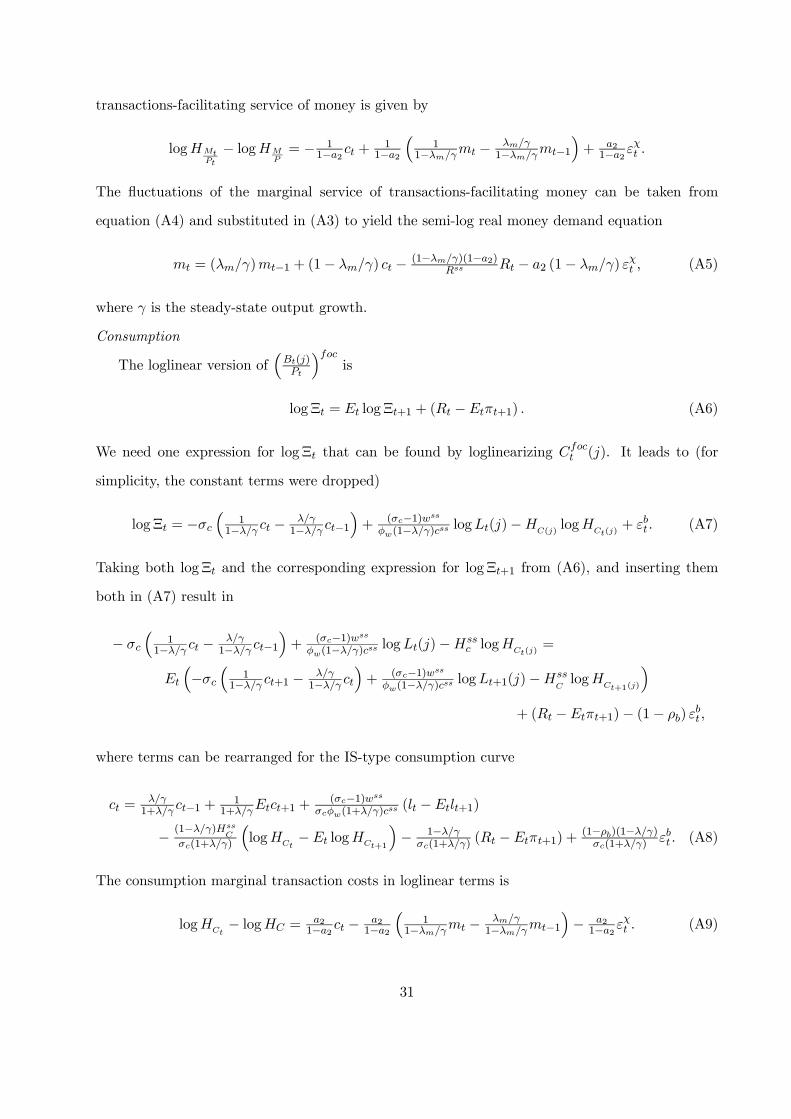
transactions-facilitating service of money is given by

logHMtPt

− logHMP= − 1

1−a2 ct +1

1−a2³

11−λm/γmt − λm/γ

1−λm/γmt−1´+ a2

1−a2 εχt .

The fluctuations of the marginal service of transactions-facilitating money can be taken from

equation (A4) and substituted in (A3) to yield the semi-log real money demand equation

mt = (λm/γ)mt−1 + (1− λm/γ) ct − (1−λm/γ)(1−a2)Rss Rt − a2 (1− λm/γ) ε

χt , (A5)

where γ is the steady-state output growth.

Consumption

The loglinear version of³Bt(j)Pt

´focis

logΞt = Et logΞt+1 + (Rt −Etπt+1) . (A6)

We need one expression for logΞt that can be found by loglinearizing Cfoct (j). It leads to (for

simplicity, the constant terms were dropped)

logΞt = −σc³

11−λ/γ ct − λ/γ

1−λ/γ ct−1´+ (σc−1)wss

φw(1−λ/γ)css logLt(j)−HC(j)

logHCt(j)

+ εbt . (A7)

Taking both logΞt and the corresponding expression for logΞt+1 from (A6), and inserting them

both in (A7) result in

− σc

³1

1−λ/γ ct − λ/γ1−λ/γ ct−1

´+ (σc−1)wss

φw(1−λ/γ)css logLt(j)−Hssc logHCt(j)

=

Et

³−σc

³1

1−λ/γ ct+1 − λ/γ1−λ/γ ct

´+ (σc−1)wss

φw(1−λ/γ)css logLt+1(j)−HssClogH

Ct+1(j)

´+ (Rt −Etπt+1)− (1− ρb) ε

bt ,

where terms can be rearranged for the IS-type consumption curve

ct =λ/γ1+λ/γ ct−1 +

11+λ/γEtct+1 +

(σc−1)wssσcφw(1+λ/γ)c

ss (lt −Etlt+1)

− (1−λ/γ)HssC

σc(1+λ/γ)

³logHCt

−Et logHCt+1

´− 1−λ/γ

σc(1+λ/γ)(Rt −Etπt+1) +

(1−ρb)(1−λ/γ)σc(1+λ/γ)

εbt . (A8)

The consumption marginal transaction costs in loglinear terms is

logHCt− logHC =

a21−a2 ct − a2

1−a2³

11−λm/γmt − λm/γ

1−λm/γmt−1´− a2

1−a2 εχt . (A9)

31

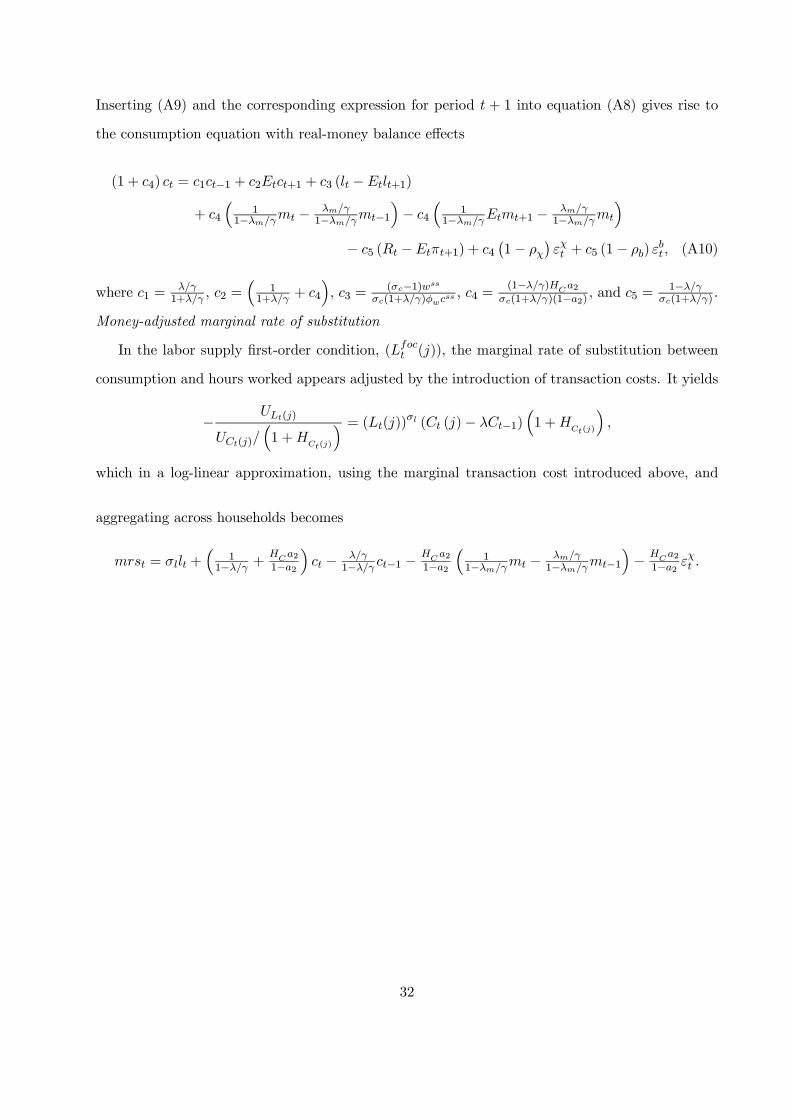
Inserting (A9) and the corresponding expression for period t + 1 into equation (A8) gives rise to

the consumption equation with real-money balance effects

(1 + c4) ct = c1ct−1 + c2Etct+1 + c3 (lt −Etlt+1)

+ c4

³1

1−λm/γmt − λm/γ1−λm/γmt−1

´− c4

³1

1−λm/γEtmt+1 − λm/γ1−λm/γmt

´− c5 (Rt −Etπt+1) + c4

¡1− ρχ

¢εχt + c5 (1− ρb) ε

bt , (A10)

where c1 =λ/γ1+λ/γ , c2 =

³1

1+λ/γ + c4

´, c3 =

(σc−1)wssσc(1+λ/γ)φwc

ss , c4 =(1−λ/γ)HC a2

σc(1+λ/γ)(1−a2) , and c5 =1−λ/γ

σc(1+λ/γ).

Money-adjusted marginal rate of substitution

In the labor supply first-order condition, (Lfoct (j)), the marginal rate of substitution between

consumption and hours worked appears adjusted by the introduction of transaction costs. It yields

− ULt(j)

UCt(j)/³1 +H

Ct(j)

´ = (Lt(j))σl (Ct (j)− λCt−1)

³1 +H

Ct(j)

´,

which in a log-linear approximation, using the marginal transaction cost introduced above, and

aggregating across households becomes

mrst = σllt +³

11−λ/γ +

HC a21−a2

´ct − λ/γ

1−λ/γ ct−1 −HC a21−a2

³1

1−λm/γmt − λm/γ1−λm/γmt−1

´− HC a2

1−a2 εχt .

32

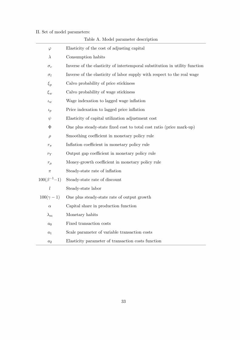
II. Set of model parameters:

Table A. Model parameter description

ϕ Elasticity of the cost of adjusting capital

λ Consumption habits

σc Inverse of the elasticity of intertemporal substitution in utility function

σl Inverse of the elasticity of labor supply with respect to the real wage

ξp Calvo probability of price stickiness

ξw Calvo probability of wage stickiness

ιw Wage indexation to lagged wage inflation

ιp Price indexation to lagged price inflation

ψ Elasticity of capital utilization adjustment cost

Φ One plus steady-state fixed cost to total cost ratio (price mark-up)

ρ Smoothing coefficient in monetary policy rule

rπ Inflation coefficient in monetary policy rule

rY Output gap coefficient in monetary policy rule

rμ Money-growth coefficient in monetary policy rule

π Steady-state rate of inflation

100(β−1−1) Steady-state rate of discount

l Steady-state labor

100(γ − 1) One plus steady-state rate of output growth

α Capital share in production function

λm Monetary habits

a0 Fixed transaction costs

a1 Scale parameter of variable transaction costs

a2 Elasticity parameter of transaction costs function

33

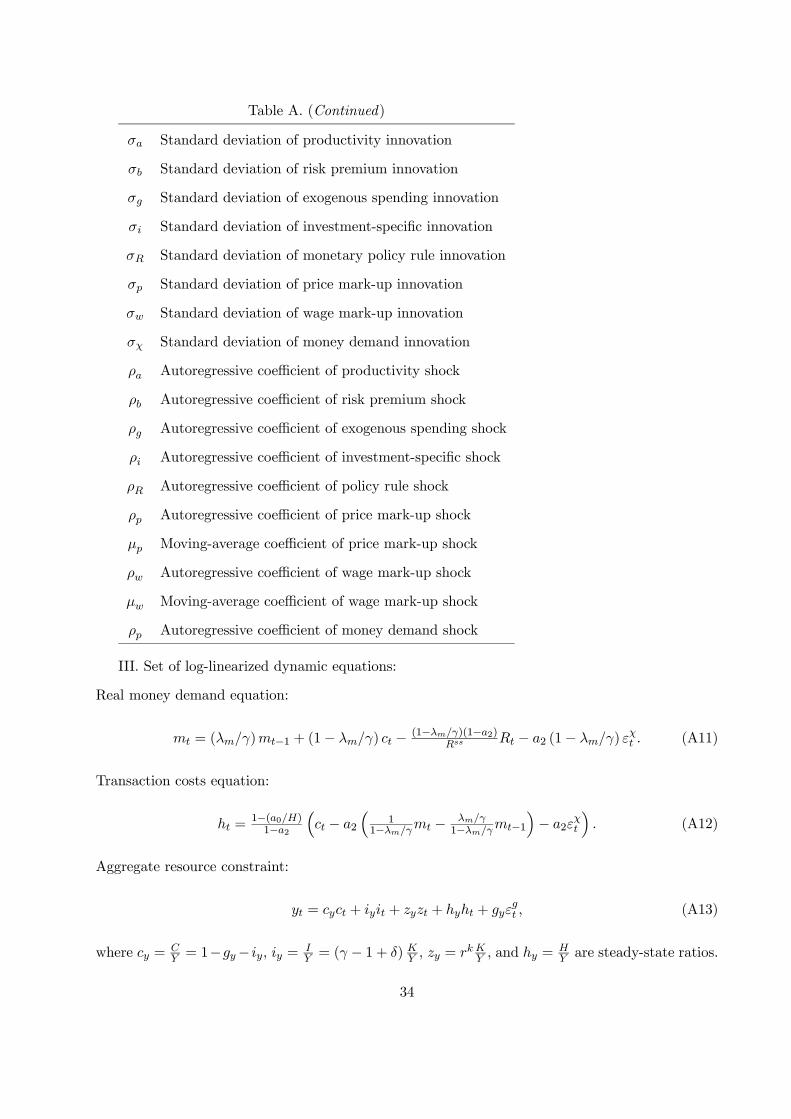
Table A. (Continued)

σa Standard deviation of productivity innovation

σb Standard deviation of risk premium innovation

σg Standard deviation of exogenous spending innovation

σi Standard deviation of investment-specific innovation

σR Standard deviation of monetary policy rule innovation

σp Standard deviation of price mark-up innovation

σw Standard deviation of wage mark-up innovation

σχ Standard deviation of money demand innovation

ρa Autoregressive coefficient of productivity shock

ρb Autoregressive coefficient of risk premium shock

ρg Autoregressive coefficient of exogenous spending shock

ρi Autoregressive coefficient of investment-specific shock

ρR Autoregressive coefficient of policy rule shock

ρp Autoregressive coefficient of price mark-up shock

μp Moving-average coefficient of price mark-up shock

ρw Autoregressive coefficient of wage mark-up shock

μw Moving-average coefficient of wage mark-up shock

ρp Autoregressive coefficient of money demand shock

III. Set of log-linearized dynamic equations:

Real money demand equation:

mt = (λm/γ)mt−1 + (1− λm/γ) ct − (1−λm/γ)(1−a2)Rss Rt − a2 (1− λm/γ) ε

χt . (A11)

Transaction costs equation:

ht =1−(a0/H)1−a2

³ct − a2

³1

1−λm/γmt − λm/γ1−λm/γmt−1

´− a2ε

χt

´. (A12)

Aggregate resource constraint:

yt = cyct + iyit + zyzt + hyht + gyεgt , (A13)

where cy = CY = 1−gy− iy, iy = I

Y = (γ − 1 + δ) KY , zy = rk KY , and hy =HY are steady-state ratios.

34

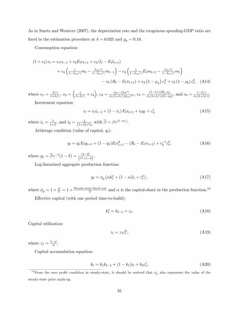
As in Smets and Wouters (2007), the depreciation rate and the exogenous spending-GDP ratio are

fixed in the estimation procedure at δ = 0.025 and gy = 0.18.

Consumption equation:

(1 + c4) ct = c1ct−1 + c2Etct+1 + c3 (lt −Etlt+1)

+ c4

³1

1−λm/γmt − λm/γ1−λm/γmt−1

´− c4

³1

1−λm/γEtmt+1 − λm/γ1−λm/γmt

´− c5 (Rt −Etπt+1) + c4

¡1− ρχ

¢εχt + c5 (1− ρb) ε

bt , (A14)

where c1 =λ/γ1+λ/γ , c2 =

³1

1+λ/γ + c4

´, c3 =

(σc−1)wssσc(1+λ/γ)φwc

ss , c4 =(1−λ/γ)HC a2

σc(1+λ/γ)(1−a2) , and c5 =1−λ/γ

σc(1+λ/γ)

Investment equation:

it = i1it−1 + (1− i1)Etit+1 + i2qt + εit, (A15)

where i1 = 11+β

, and i2 =1

(1+β)γ2ϕwith β = βγ(1−σc).

Arbitrage condition (value of capital, qt):

qt = q1Etqt+1 + (1− q1)Etrkt+1 − (Rt −Etπt+1) + c−13 εbt , (A16)

where q1 = βγ−1(1− δ) = (1−δ)(rk+1−δ) .

Log-linearized aggregate production function:

yt = φp (αkst + (1− α)lt + εat ) , (A17)

where φp = 1+φY = 1+

Steady-state fixed costY and α is the capital-share in the production function.16

Effective capital (with one period time-to-build):

kst = kt−1 + zt. (A18)

Capital utilization:

zt = z1rkt , (A19)

where z1 =1−ψψ .

Capital accumulation equation:

kt = k1kt−1 + (1− k1)it + k2εit, (A20)

16From the zero profit condition in steady-state, it should be noticed that φp also represents the value of the

steady-state price mark-up.

35

where k1 = 1−δγ and k2 =

³1− 1−δ

γ

´¡1 + β

¢γ2ϕ.

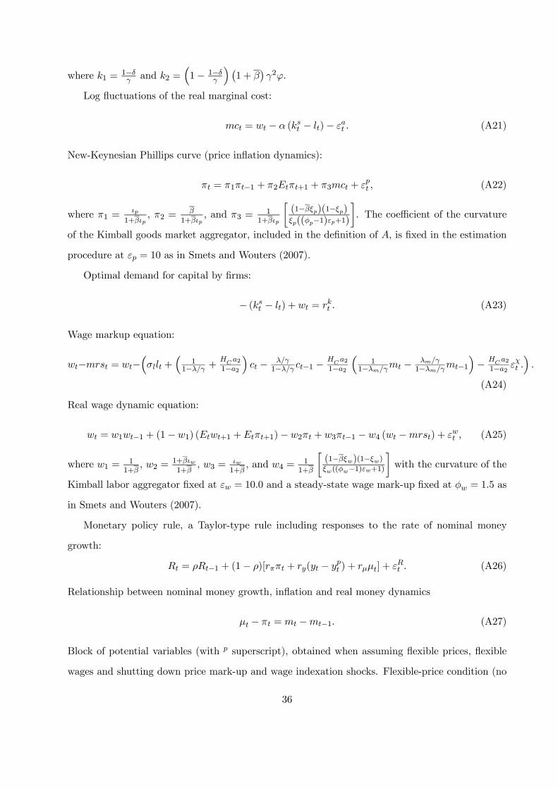
Log fluctuations of the real marginal cost:

mct = wt − α (kst − lt)− εat . (A21)

New-Keynesian Phillips curve (price inflation dynamics):

πt = π1πt−1 + π2Etπt+1 + π3mct + εpt , (A22)

where π1 =ιp

1+βιp, π2 =

β

1+βιp, and π3 =

11+βιp

∙(1−βξp)(1−ξp)ξp((φp−1)εp+1)

¸. The coefficient of the curvature

of the Kimball goods market aggregator, included in the definition of A, is fixed in the estimation

procedure at εp = 10 as in Smets and Wouters (2007).

Optimal demand for capital by firms:

− (kst − lt) + wt = rkt . (A23)

Wage markup equation:

wt−mrst = wt−³σllt +

³1

1−λ/γ +HC a21−a2

´ct − λ/γ

1−λ/γ ct−1 −HC a21−a2

³1

1−λm/γmt − λm/γ1−λm/γmt−1

´− HC a2

1−a2 εχt .´.

(A24)

Real wage dynamic equation:

wt = w1wt−1 + (1−w1) (Etwt+1 +Etπt+1)− w2πt + w3πt−1 − w4 (wt −mrst) + εwt , (A25)

where w1 = 11+β

, w2 =1+βιw1+β

, w3 = ιw1+β

, and w4 =11+β

∙(1−βξw)(1−ξw)ξw((φw−1)εw+1)

¸with the curvature of the

Kimball labor aggregator fixed at εw = 10.0 and a steady-state wage mark-up fixed at φw = 1.5 as

in Smets and Wouters (2007).

Monetary policy rule, a Taylor-type rule including responses to the rate of nominal money

growth:

Rt = ρRt−1 + (1− ρ)[rππt + ry(yt − ypt ) + rμμt] + εRt . (A26)

Relationship between nominal money growth, inflation and real money dynamics

μt − πt = mt −mt−1. (A27)

Block of potential variables (with p superscript), obtained when assuming flexible prices, flexible

wages and shutting down price mark-up and wage indexation shocks. Flexible-price condition (no

36

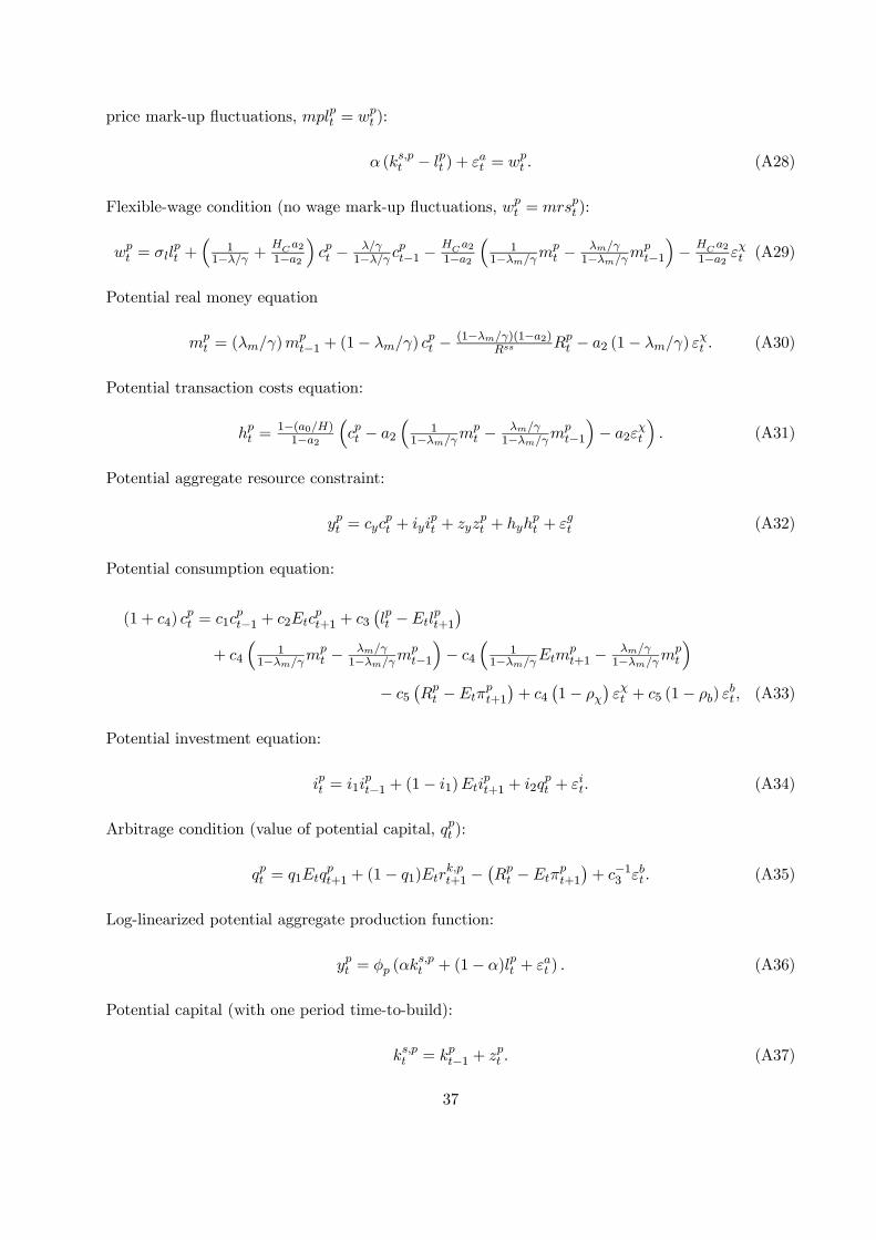
price mark-up fluctuations, mplpt = wpt ):

α (ks,pt − lpt ) + εat = wpt . (A28)

Flexible-wage condition (no wage mark-up fluctuations, wpt = mrspt ):

wpt = σll

pt +

³1

1−λ/γ +HCa2

1−a2´cpt − λ/γ

1−λ/γ cpt−1 −

HCa2

1−a2³

11−λm/γm

pt − λm/γ

1−λm/γmpt−1´− H

Ca2

1−a2 εχt (A29)

Potential real money equation

mpt = (λm/γ)m

pt−1 + (1− λm/γ) c

pt − (1−λm/γ)(1−a2)

Rss Rpt − a2 (1− λm/γ) ε

χt . (A30)

Potential transaction costs equation:

hpt =1−(a0/H)1−a2

³cpt − a2

³1

1−λm/γmpt − λm/γ

1−λm/γmpt−1´− a2ε

χt

´. (A31)

Potential aggregate resource constraint:

ypt = cycpt + iyi

pt + zyz

pt + hyh

pt + εgt (A32)

Potential consumption equation:

(1 + c4) cpt = c1c

pt−1 + c2Etc

pt+1 + c3

¡lpt −Etl

pt+1

¢+ c4

³1

1−λm/γmpt − λm/γ

1−λm/γmpt−1´− c4

³1

1−λm/γEtmpt+1 − λm/γ

1−λm/γmpt

´− c5

¡Rpt −Etπ

pt+1

¢+ c4

¡1− ρχ

¢εχt + c5 (1− ρb) ε

bt , (A33)

Potential investment equation:

ipt = i1ipt−1 + (1− i1)Eti

pt+1 + i2q

pt + εit. (A34)

Arbitrage condition (value of potential capital, qpt ):

qpt = q1Etqpt+1 + (1− q1)Etr

k,pt+1 −

¡Rpt −Etπ

pt+1

¢+ c−13 εbt . (A35)

Log-linearized potential aggregate production function:

ypt = φp (αks,pt + (1− α)lpt + εat ) . (A36)

Potential capital (with one period time-to-build):

ks,pt = kpt−1 + zpt . (A37)

37

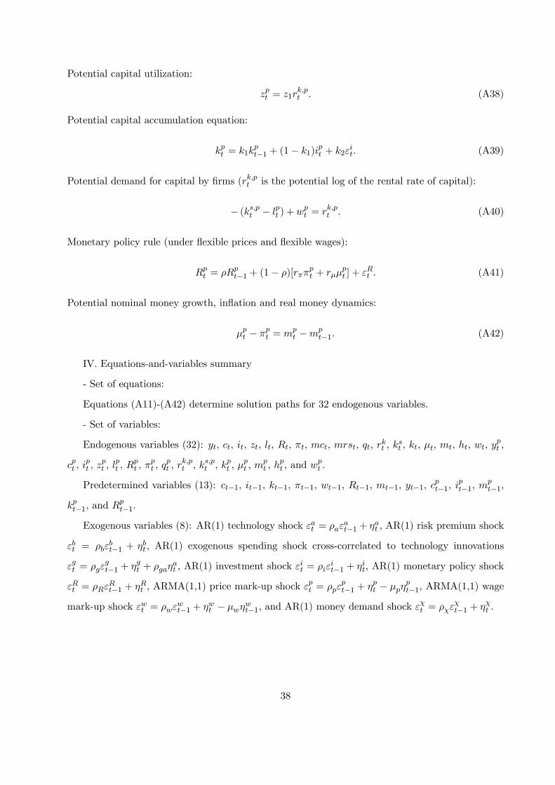
Potential capital utilization:

zpt = z1rk,pt . (A38)

Potential capital accumulation equation:

kpt = k1kpt−1 + (1− k1)i

pt + k2ε

it. (A39)

Potential demand for capital by firms (rk,pt is the potential log of the rental rate of capital):

− (ks,pt − lpt ) +wpt = rk,pt . (A40)

Monetary policy rule (under flexible prices and flexible wages):

Rpt = ρRp

t−1 + (1− ρ)[rππpt + rμμ

pt ] + εRt . (A41)

Potential nominal money growth, inflation and real money dynamics:

μpt − πpt = mpt −mp

t−1. (A42)

IV. Equations-and-variables summary

- Set of equations:

Equations (A11)-(A42) determine solution paths for 32 endogenous variables.

- Set of variables:

Endogenous variables (32): yt, ct, it, zt, lt, Rt, πt, mct, mrst, qt, rkt , kst , kt, μt, mt, ht, wt, y

pt ,

cpt , ipt , z

pt , l

pt , R

pt , π

pt , q

pt , r

k,pt , ks,pt , k

pt , μ

pt , m

pt , h

pt , and wp

t .

Predetermined variables (13): ct−1, it−1, kt−1, πt−1, wt−1, Rt−1, mt−1, yt−1, cpt−1, ipt−1, m

pt−1,

kpt−1, and Rpt−1.

Exogenous variables (8): AR(1) technology shock εat = ρaεat−1 + ηat , AR(1) risk premium shock

εbt = ρbεbt−1 + ηbt , AR(1) exogenous spending shock cross-correlated to technology innovations

εgt = ρgεgt−1 + ηgt + ρgaη

at , AR(1) investment shock εit = ρiε

it−1 + ηit, AR(1) monetary policy shock

εRt = ρRεRt−1 + ηRt , ARMA(1,1) price mark-up shock εpt = ρpε

pt−1 + ηpt − μpη

pt−1, ARMA(1,1) wage

mark-up shock εwt = ρwεwt−1 + ηwt − μwη

wt−1, and AR(1) money demand shock ε

χt = ρχε

χt−1 + ηχt .

38