Embed Size (px)
Citation preview

A study of damping in fiber-reinforced composites
Rakesh Chandraa, S.P. Singhb,*, K. Guptac
aDr. B.R.A. Regional Engineering College, Jalandhar, Indiab Department of Mechanical Engineering, Indian Institute of Technology, New Delhi 110 016, India
0Indian Institute of Technology, Delhi 110 016, India
Received 9 January 2002; accepted 13 January 2003
Abstract
Damping contributions from the viscoelastic matrix, interphase and the dissipation resulting fromdamage sites are considered to evaluate composite material damping coefficients in various loading modes.The paper presents the results of the FEM/Strain energy investigations carried out to predict anisotropic-damping matrix comprising of loss factors Z11, Z22, Z12 a nd Z23 considering the dissipation of energy due tofiber and matrix (two phase) and correlate the same with various micromechanical theories. Damping inthree phase (i.e., fiber-interphase-matrix) composite is also calculated as an attempt to understand theeffect of interphase. The contribution of energy dissipation due to sliding at the fiber-matrix interface isincorporated to evaluate its effect on Z11, Z22, Z12 a nd Z23 in fiber-reinforced composite having damage inthe form of hairline debonding. Comparative studies of the various micromechanical theories/models withFEM/Strain energy method for the prediction of damping coefficients have shown consistency when boththe effect of variable nature of stress and the fiber interaction is considered. Parametric damping studies forthree phase composite have shown that the change in properties of fiber, matrix and interphase leads to achange in the magnitude of effectiveness of interphase, but the manner in which the interphase would affectthe various loss factors depends predominately upon whether the hard or soft interphase is chosen. Analysisof the effect of damage on composite damping indicates that it is sensitive to its orientation and type ofloading.
1. Introduction
Damping is an important parameter related to dynamic behavior of fiber-reinforced compositestructures. The successful characterization of dynamic response of viscoelastically damped

476 R. Chandra et al. / Journal of Sound and Vibration 262 (2003) 475-496
composite materials to prescribed modes of loading and time histories depends upon use of anappropriate analytical model/method, describing properties of composites based upon itsconstituents and their interaction, condition of interphase, presence of defects and selection ofcomputational techniques. Composites are anisotropic and non-uniform bodies and a descriptionof damping process in these materials calls for essential new development in the theory ofdamping. Zioniev and Ermakov [1] have classified the studies on composites as experimentalinvestigations to generate damping data, the value and meaning of damping characteristics, theirrelation with material internal structure and development of damping theories/models in order tofully describe the energy dissipation process in composite materials. The mechanisms to which thedissipation energy can be attributed are: the viscoelastic nature of the matrix and/or fibermaterials, damping due to interphase [2], damping due to damage [3], and viscoelastic damping atlarge amplitudes of vibration or high stress/strain levels and thermoelastic damping [4].
The effect of various damping mechanisms has been taken care of either individually or incombination, while modelling damping in fiber-reinforced composites. Chang and Bert [5], Cremaand Castellani [6], Saravanos and Chamis [7,8], Kaliske and Rother [9], Chandra et al. [10,11]have predicted damping coefficients of fiber-reinforced composites considering the dissipation ofenergy due to fiber and matrix only whereby referring to it as a two-phase composite.
The contribution of three phases i.e., fiber-interphase-matrix in composites towards dampingevaluation has been studied by Chaturvedi and Tzeng [12], Vantomme [13], Gibson et al. [2],Finegan and Gibson [14], and Chandra [15] and is incorporated in damping models. Further, theeffect of damage is modelled by the finite element approach using a 2-D friction element. Apseudo dynamic approach is proposed to predict total loss factors of composites for differentloadings for a single fiber-matrix debonding [15]. An integrated approach to study the effect offiber-matrix, interphase and the dissipation resulting from damage sites at the fiber-matrixinterface on the damping are considered here for fiber-reinforced composites. This has beenachieved using FEM models developed for the two-phase composites and upgrading the same forthe composite with interphase and damage.
2. Composite damping mechanisms
A detailed review of the damping studies in fiber-reinforced composites is given by Chandraet al. [16]. Different sources of energy dissipation in fiber-reinforced composites are brieflydiscussed below.
(1) Viscoelastic nature of matrix and/or fiber materials: the major contribution to compositedamping is due to the matrix. However, fiber damping must be included in the analysis for carbonand Kevlar fibers, which have higher damping as compared to other types of fibers. Dampingmodels, which consider the effect of dissipation of energy due to fiber and matrix in fiber-reinforced composite, are called two-phase models.
(2) Damping due to interphase: interphase [2] is the region adjacent to the fiber surface all alongthe fiber length. The interphase possesses a considerable thickness and its properties are differentfrom those of embedded fiber and bulk matrix. The nature of interphase: weak, ideal or strongaccordingly affects the mechanical properties and in turn damping of the fiber-reinforced

R. Chandra et al. / Journal of Sound and Vibration 262 (2003) 475-496 477
composites. Changing composite material comprised of fiber-interphase-matrix leads tomodification of its overall damping.
(3) Damping due to damage: it is mainly of two types: (i) frictional damping due to slip inunbound regions between fiber and matrix interface or delaminations, and (ii) damping due todissipation in the area of matrix cracks, broken fibers, etc.
Increase in damping due to fiber-matrix interfacial slip is reported to be significant [3]. Also,damping is more sensitive than stiffness to damage in a composite [17].
(4) Viscoelastic damping at large amplitudes of vibration or high stress/strain levels exhibits anevident degree of non-linear damping due to the presence of high stress and strain concentrationin the local regions between fibers [4].
(5) Thermoplastic damping is due to cyclic heat flow from the region of compressive stress tothe region of tensile stress in the composite, especially in thermoplastic composites [18].
Damping studies considering the composite as two-phase or three-phase systems and modellingof damage at the fiber matrix interface for damping is reported as an integrated approach in thispaper.
3. Analysis for damping
Micromechanical damping analysis of unidirectional fiber-reinforced composites involves thedetermination of contribution of its constituents, i.e., fiber, matrix, interphase and condition ofthe fiber-matrix interface. In this paper, initially it is presumed that there is perfect bondingbetween fiber and matrix, and the composite is considered to be made up of two phases (fiber-matrix). The concept developed for a two-phase model is extended to three-phase composites(fiber-interphase-matrix). Further, the effect of the condition of fiber-matrix interface, i.e.,damage (micro-crack) or discontinuity at the fiber-matrix interface is incorporated in the two-phase composites.
3.1. Two- and three-phase damping models
The strain energy method proposed by Ungar and Kerwin [19] expresses, for a given loading,the composite loss factor as the ratio of the summation over all elements of the structure of theproduct of the loss factor for each element and the strain energy for each element to the totalstrain energy.
Thus the loss factor for the three-phase model considering the effect of fiber, matrix andinterphase can be expressed as
n E « Wi i

478 R. Chandra et al. / Journal of Sound and Vibration 262 (2003) 475-496
The strain energy stored in the composite under loading can be written as
Wc = 1 f OijEJ V
The total strain energy of composite can also be expressed as the sum of the contributions from itsconstituents, i.e., fiber, matrix and interphase respectively,
Wc = ðWfþWmþWiÞ: ð4Þ
The strain energy stored in the constituents, i.e., fiber matrix and interphase in a unit cell of acertain volume is given as
Wf = iWm = ±YJ{oij}l{SiJ}m{<Tij}mSVm, (6)
ij}J{SiJ}i{<Tij}iSVi. (7)
The above relationships can be modified for two-phase composite by ignoring the contribution ofthe interphase due to its absence, i.e., Wi=0 and ZI = 0. The above formulation is adopted forFEM modelling of loss factors in composite materials. Some of the important research papers ofGibson et al. [2] and Finegan and Gibson [14] made use of a FEM/Strain energy approach topredict damping in fiber-reinforced composites.
3.2. Modelling for interface damage
Damage in glass fiber-reinforced epoxy considered here is represented by a hairline crack withzero gap width at the fiber-matrix interface. Any discontinuity in the composite is referred asgeometrical non-linearity. This discontinuity at the fiber-matrix interface is modelled byapplication of a non-linear gap element. Thus, the FEM modelling of interfacial discontinuity isconsidered as non-linear. The gap element facilitates modelling of a discontinuity at the interfacewithout or with the consideration of friction, respectively. As under dynamic loading, the fiber-matrix interface is bound to dissipate energy at the debonded region, it is appropriate to usefriction elements to simulate the actual conditions. Further, in order to predict dissipation ofenergy per cycle, the non-linear/FEM model is subjected to static loads in steps varying from zeroto maximum and to zero for a half load cycle during which the crack is in a closed condition.Hence, it is through the analysis of the set of static/non-linear FEM models that energydissipation at the fiber-matrix interface is predicted.
A 2-D gap/friction element, which is a two noded non-linear element, provides node-to-nodecontact between the two bodies. The friction element is based on the law of friction relating thetangential (Ft) and normal (Fn) forces through a coefficient of friction (m). In order to predict thedissipation of energy for one cycle due to sliding at the fiber-matrix interface caused bydiscontinuity (damage), the FEM model with an interface friction element is simulated fordynamic steady state loading. For this purpose, a sinusoidally varying load is applied to thecomposite. At various stages of the load the state of the composite is analyzed with respect to theforces and displacements in the damage region. The force-displacement variation over a completecycle of loading is used to calculate the energy dissipated in the gap element. This approach is

R. Chandra et al. / Journal of Sound and Vibration 262 (2003) 475-496 479
pseudo-dynamic in nature since inertia effects are not considered and the dynamic loading isassumed as a series of static forces varying in a sinusoidal manner. Thus the force applied, Fi
varies as given in Eq. (8). A static non-linear FEM analysis is conducted for a number of discretevalues of this force:
Fi = F0 Sin ot = F0 Sin y: ð8Þ
In the process of dynamic simulation, it is necessary to select the direction and magnitude of theexcitation load for the static non-linear analysis. Here, non-linearity is introduced due to thegeometric discontinuity, i.e., debonding at the fiber-matrix interface. The magnitude of amplitudeF0 is decided on the basis of linear elastic behavior of the glass fiber-reinforced composite (GFRE)for which the damping studies are under consideration. The excitation load for the correspondingstatic non-linear FEM models simulating the dynamic behavior under particular loadingcondition is increased gradually, starting from zero in a step increment of a certain fixedpercentage of F0.
In the process of performing a sensitivity analysis of the frictional element, it is observed thatthe gap remains in closed status for half of the loading cycle, while for the remaining half it attainsan open status [15]. The dissipation of energy due to relative sliding at the fiber-matrix interfacenaturally occurs during the closed status of the discontinuity when the gap is in a sliding modedepending upon the instantaneous direction of the step load. Hence, for each type of loading, i.e.,transverse, transverse shear, extensional and in-plane shear, it is important to select the directionof the load vector so that the relative sliding occurs between the nodes of the friction elementbelonging to fiber and matrix during a particular step load. The pseudo-dynamic approach isproposed to predict the contribution of energy dissipation due to sliding at the fiber-matrixinterface. The steady state response of the FEM model is simulated by the application of loadsteps lying on a sinusoidal quarter cycle such that 0PFIPF0, where Fi is step load and F0 isamplitude of the steady state load. Dissipation of energy due to the discontinuity at the interface isobtained by varying the step load from 0 to F0 and then to 0 for half the cycle or for the quartercycle with a step load from 0 to F0 and analyzing the respective FEM models.
The output of the static non-linear FEM analysis for each load step provides Ft and the relativedisplacement ds between the nodes of the friction element simulating the discontinuity at theinterface. The area under the curve plotted between Ft vs ds gives the dissipation of energy due tothe interface for the quarter cycle. Thus, the energy dissipated per cycle at the interface due to thediscontinuity is given by
D = 2 x (I x Ft x dsÞ: ð9Þ
The total loss factor of the composite can be determined as the ratio of total energy dissipated andthe maximum strain energy per cycle as
ntotal = ^ • d o )
Here j= index of friction element, n being their total number, Df and Dm = energy dissipated byfiber and matrix, respectively, Did= energy dissipation due to individual discontinuity at theinterface, and Wid= total strain energy with interfacial discontinuity.
480 R. Chandra et al. / Journal of Sound and Vibration 262 (2003) 475-496
The contribution of the fiber-matrix can be expressed in terms of the loss factor and strainenergy without consideration of fiber-matrix interface friction (m = 0) as
ðDf þ DmÞ = ZwfWid; ð11Þ
where Zwf= loss factor without the consideration of friction at the interface.Thus, Eq. (10) can be rewritten as
otal — ð12Þ
3.3. FEM modelling
FEM models for GFRE with various fiber volume fractions are constructed and subjected todifferent types of loading conditions. 2-D, 3-D static and 2-D static non-linear (with gap/frictionelement) FEM models are analyzed for the prediction of loss factors (Z11, Z22, Z12 and Z23) for two-and three-phase models of composites with damage, respectively.
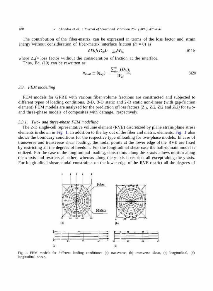
3.3.1. Two- and three-phase FEM modellingThe 2-D single-cell representative volume element (RVE) discretized by plane strain/plane stress
elements is shown in Fig. 1. In addition to the lay out of the fiber and matrix elements, Fig. 1 alsoshows the boundary conditions for the respective type of loading for two-phase models. In case oftransverse and transverse shear loading, the nodal points at the lower edge of the RVE are fixedby restricting all the degrees of freedom. For the longitudinal shear case the half-domain model isutilized. For the case of the longitudinal loading, constraints along the x-axis allows motion alongthe x-axis and restricts all other, whereas along the y-axis it restricts all except along the y-axis.For longitudinal shear, nodal constraints on the lower edge of the RVE restrict all the degrees of
Zi 2S Z £ Z i "
(b)
k\ S3 Mi
Fig. 1. FEM models for different loading conditions: (a) transverse, (b) transverse shear, (c) longitudinal, (d)longitudinal shear.

R. Chandra et al. / Journal of Sound and Vibration 262 (2003) 475-496 481
(a)Interphase
Fig. 2. 2-D FEM models with interphase for Vf = 0:4 (fixed), Vi = 0 :1 ; Vm = 0:5; number of elements Nf = 1264 ;
Ni — 65296 ; and Nm — 972130 : Loading conditions: (a) transverse and (b) transverse shear.
Table 1Basic properties of GFRE constituents
Properties E-glass fiber Epoxy matrix Hard-interphase Soft-interphase
E (Gpa)G (Gpa)V
n
72.430.20.20.0018
2.761.020.350.015
37.5815.610.2040.0084
0.50.1780.40.0084
freedom. Transverse uniform stress is applied at nodal points along the y-axis (Fig. 1(a)), whereastransverse shear acts on the face of the elements (Fig. 1(b)). Similarly, the nodal longitudinal stressis applied at the nodes perpendicular to the face of the respective element (Fig. 1(c)) for the case ofthe longitudinal model while longitudinal shear stress acts on the face of the elements (Fig. 1(d)) incase of longitudinal shear models, respectively. The analysis of the FEM models was performedfor the prediction of the state of stress in the constituents of the composite. The strain energystored in the fiber and matrix, and the loss factors for different loading conditions are obtainedbased on Eqs. (4)-(7). Strain energy is determined in the present study over the area of eachelement assuming a unit constant thickness. These two-phase FEM models have been modified byintroducing an interphase between fiber and the matrix to predict its effect on composite damping.
2-D FEM models with interphase volume fraction Vi = 0.02, 0.04, 0.08 and 0.1 for transverseand transverse shear loading with single-cell square array packing are analyzed. Fig. 2(a) and (b)show the 2-D FEM model for transverse and transverse shear loadings, respectively. These modelsare constructed for a fixed fiber volume fraction Vf= 0.4 considering the interphase to be (1) hard:interphase properties are taken as average of the elastic properties of fiber and matrix; or (2) soft:interphase properties are lower than those of the matrix (see Table 1). This assumption is madebecause a precise estimation of the properties of the interphase is not available in the reportedliterature [12-13]. Similarly, the loss factor for both the soft and hard interphase is assumed to bethe average of the loss factor of fiber and matrix, because no theoretical or experimental data isavailable in literature. Chaturvedi and Tzeng [12] assumed the loss factor of the interphase to beequal to that of the matrix because of a lack of information in this regard. Loss factors in

482 R. Chandra et al. / Journal of Sound and Vibration 262 (2003) 475-496
Matrix
Interphase
Matrix
Interphase
Fig. 3. 3-D FEM model for composite with interphase: Vf = 0:4 (fixed), Vi — 0 :1 ; number of elements Nf = 12270;
Ni — 2712510; and Nm — 5112690: Loading conditions: (a) transverse, and (b) transverse shear.
transverse and transverse shear, longitudinal and longitudinal shear modes are also predictedusing 3-D FEM models. 3-D FEM models with an interphase for transverse and transverse shearloading are shown in Fig. 3. Hexahedra eight noded elements are used to construct the FEMmodel for the fiber-reinforced composite with a fiber volume fraction Vf=0.4 [15].
The total thickness of the interphase (Ti) is worked out such that the maximum value of Vi = 0.1is further subdivided into a number of layers to obtain Vi = 0.02, 0.04, 0.08. A finer mesh size isused in the interphase near the fiber as well as near the matrix in order to correctly predict stressesin interphase region. Both a soft and a hard interphase is incorporated in the FEM models. Theoutput of the static analysis of these FEM models is obtained in the form of the strain energy forthe finite elements of fiber, matrix and interphase in the respective mode of loading. The strainenergy of the constituent elements is determined using Eqs. (4)-(7) and corresponding loss factors
23) a r e predicted.
3.3.2. FEM modelling for damageThe interfacial discontinuity is modelled by single- and multiple-gap elements in case of
transverse and transverse shear loading to study the effect of orientation as well as the effect of thenumber of gap elements for the same gap size. The orientation of gap yg is defined as anglesubtended by the direction of the gap at the coincident nodes with respect to the global x-axis. Thegap size ygs is referred as the included angle between the extreme merged nodes corresponding tobeginning and end of the discontinuity. Thus the discontinuity is characterized by parameters: gapwidth (GW), gap size (ygs) number of gap elements and gap orientation (yg). In case of the single-gap element model, the orientation of gap coincides with the axis of symmetry of the gap, whereasfor the multiple gap element model, an average gap orientation is considered which again refers tothe axis of the symmetry of the gap. Single-gap element refers to use of only one friction elementbetween a debonded fiber and the matrix interface. The three-gap element FEM modelincorporates, for the same gap size, three friction elements.
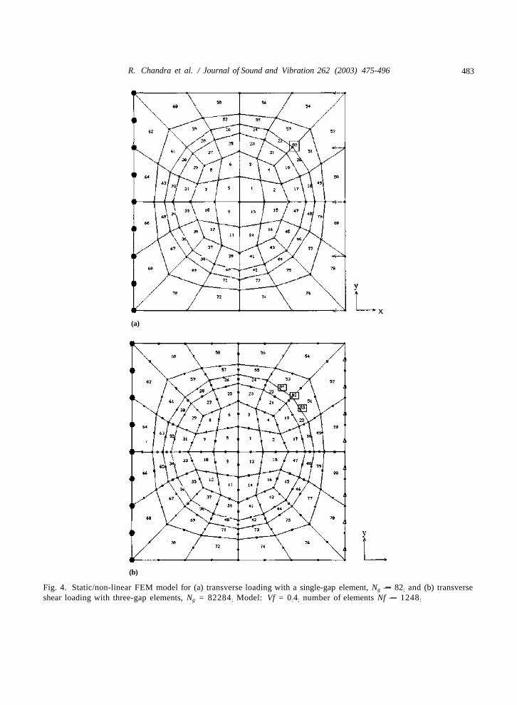
A representative FEM model for transverse loading with a single-gap element having yg = 45°and ygs=45° is shown in Fig. 4(a). It consists of 80 quadrilateral four noded elements comprised ofa number of elements in the fiber (Nf) from 1 to 48, and elements in the matrix (Nm) from 49 to 80,
R. Chandra et al. / Journal of Sound and Vibration 262 (2003) 475-496 483
(a)
(b)
Fig. 4. Static/non-linear FEM model for (a) transverse loading with a single-gap element, Ng — 82; and (b) transverseshear loading with three-gap elements, Ng = 82284 : Model: Vf = 0:4; number of elements Nf — 1248 :

484 R. Chandra et al. / Journal of Sound and Vibration 262 (2003) 475-496
in addition to one friction element, Ng = 82. The model is analyzed for several load steps Fi whichis increased gradually from 0 to 1N in an increment of 0.1 such that 0PF0PFI. The correspondingoutput Ft, ds, Wf and Wm is recorded.
Various static non-linear FEM models, also with a single-gap element for different gaporientations, yg varying from 0 to 180° in step of 22.5°, are analyzed in combination with apseudo dynamic approach to obtain strain energy of the constituent finite element and the energydissipated at the interface due to debonding in different loading conditions. Fig. 4(a) alsoelaborates how the single-gap element is incorporated in the various FEM models to study theeffect of gap orientation on overall damping. The gap orientation varies from 0 to 180° in a stepof 22.5°, which refers to the direction of discontinuity at the fiber matrix interface. Three-gapelement FEM models for transverse loading are obtained by replacing single-gap elements bythree-gap elements. The purpose of using three-gap elements is to study the effect of the numberof friction (gap) elements on the dissipation of energy at the interface for the same gap size (ygs).So three friction elements are introduced along the fiber-matrix interface for the same gap size(ygs = 45°) as in case of single-gap element models. The orientation of three friction elementswithin the gap can be seen from Fig. 4(b): yg with respect to the global x-axis is 45° (position offriction element number Ng = 82) and yi = +11.25° with respect to the gap axis (position offriction element Ng = 84 and 83). Fig. 4(b) shows the static non-linear FEM model with theapplication of three-gap elements. Models with three-gap elements for different gap orientations,yg = 0 to 180° in steps of 22.5°, are analyzed for the non-linear static case and are drawn for allgap elements maintaining closed status for all step loads (0pFipF0). Energy dissipated due to slipat the interface in transverse loading for single and three-gap element models are predicted [15].Representative Ft—ds plots (for yg = O-18O°) for static/non-linear FEM models with three-gapelements under transverse loading are given in Fig. 5. Each area under these curves can beevaluated to obtain the individual contribution of gap elements to the total dissipated energy dueto the gap size ygs = 45°.
A pseudo-dynamic approach is used to predict total loss factor of composite for variousorientations of gap element. In this approach, the following procedure is adopted for all thedamping predictions for models with friction elements.
Step 1: determine the loss factor for the composite when m = 0 using Eq. (11).Step 2: plot a graph between Ft and ds for the corresponding incremental loads for 0pF0pFi.
The area under the Ft—ds curve provides the energy dissipated for the quarter cycle of the steadystate load, Ft = F0 Sin ot.
Step 3: use Eq. (12) to predict the total loss factor Z22, considering dissipation of energy due tofiber, matrix and due to sliding at the interface, i.e., friction.
The percentage increase in loss factor due to interface sliding, with respect to a pristine materialloss factor is expressed under transverse loading as
% increase in loss factor t]22 = p x 100: ð13ÞðZ22Þp
In a similar way FEM models with single/three-gap elements for the transverse shear loadingcondition and relevant boundary conditions are analyzed in order to predict the total shear lossfactor (Z23)t and the percentage increase in (Z23)t for the respective case.

R. Chandra et al. / Journal of Sound and Vibration 262 (2003) 475-496 485
3 0 2 4 6 8 1 0 0 2 4 6 8 1 0
(b) d (<=) d
xHT
0.0 0.2 0.4 0.6 0.8 0
(d) ds (e)
xlO"3
0.0 0.2 0.4 0.6 0.8
(g) ds
0 1 2 3 4 5 0 1 2 3 4 5
Fig. 5. Energy dissipated at the interface due to friction: transverse loading, three-gap element model (gap element •,GE-82; ’, GE-83; and n, GE-84) for orientation of gap axis yg (a) 0°, (b) 22.5°, (c) 45°, (d) 67.5°, (e) 90°, (f) 112.5°,(g) 135°, (h)157.5°, and (i) 180°.
Discontinuity at the fiber-matrix interface, in case of longitudinal and longitudinal shear isconsidered to be around the circumference of the fiber. Due to symmetry, a 2-D half-domainFEM model is used, and the discontinuity is modelled by a single-gap element. The position ofdiscontinuity is identified along the fiber axis by the location of the gap element, and defined as theratio x/l (Fig. 6). Here, x is the location of gap element with respect to the left edge of the modeland l is the length of the model along the fiber axis. Longitudinal or longitudinal shear loading isapplied, while analyzing the corresponding model.
Typical 2-D FEM models with single-gap element for longitudinal and longitudinal shearloading with a discontinuity starting at the extreme right hand side and showing the loading andboundary conditions are depicted in Fig. 6. Each model consists of eight noded quadrilateral

486 R. Chandra et al. / Journal of Sound and Vibration 262 (2003) 475-496
Fiber .
(a)
Matrix
4
\
|
\ 2 1
,-1\—<
22
21 <
23
3i <
24
4• <
25
5
t {
26
6
27
7
28
8
29
9
30
10
31
11 12
33
13
34
14
35
IS
36
16
37
17
38
18
39
191 <
40
20
» 1
•
41
1 •
\21
^1
22
2
23
3
24
4
25
5
26
6
27
7t 1
28
8
29
9> (
30
10> (
31
11
32
12• 1
33
131 •
34
141 <
35
IS» 1
36
161 i
37
171 <
38
181 •
39
19> <
40
20
1 \
(b)
Fig. 6. Static/non-linear FEM model with single-gap element for different loadings model; Vf — 0:4; number ofelements in fiber Nf — 1 — 20; in matrix Nm = 21 — 40 and gap element Ng — 41 : (a) Longitudinal loading, (b) shearloading.
elements: 1 to 20 in the fiber and 21-40 in the matrix. Element number 41 is a gap element at thelocation x/l= 1.
The total loss factor in extension and shear is predicted using Eqs. (11) and (12). In Eq. (12) therespective loss factors are replaced by ones corresponding to the respective loading condition.
4. Results and discussions
The total loss factor for a composite is due to the contributions of fiber, matrix and energydissipated because of sliding at the damaged interface. Results of damping predictions based onthe integrated FEM/Strain energy approach considering the above-mentioned mechanisms arepresented here.
4.1. Two-phase composite
Damping coefficients predicted by FEM/strain energy modelling and from various othermicromechanical models [7, 20-25] for two-phase composites are presented in Table 2 for a fibervolume fraction of 0.4. Table 2 shows that for the given fiber volume fraction the FEM/strainenergy prediction for Z11 compares well with those of the Saravanos-Chamis approach, and the
Table 2Comparison of loss moduli using various models/methods
Model/method Z22 Z23
EshelbyTsaiHashinHalpin-TsaiFEM/Strain energySaravanos-Chamis
9.867 x 10~4
2.514 xlO~3
2.6539 xlO~3
2.514 xlO~3
1.40593 x 101.42107x101.433 x 10~2
1.358 x 10~2
1.4495 x 10~2
1.10159x10
- 2
- 2
- 2
1.41181 xlO"
1.41 x 10~2
1.4118 xlO" 2
1.4712 xlO" 2
1.10159x10"
1.43321 x
1.4489 x 10"1.0544 x 10"
R. Chandra et al. / Journal of Sound and Vibration 262 (2003) 475-496 487
Hashin model also indicates that the predictions made by Eshelby's method are not accurateenough. Loss factors Z22, Z12 and Z23 predicted by the FEM/strain energy method correlate verywell. A detailed comparative study of damping predictions by the FEM/strain energy method inreference to other models/methods has been studied by the authors and reported previously [25].
4.2. Three-phase composites
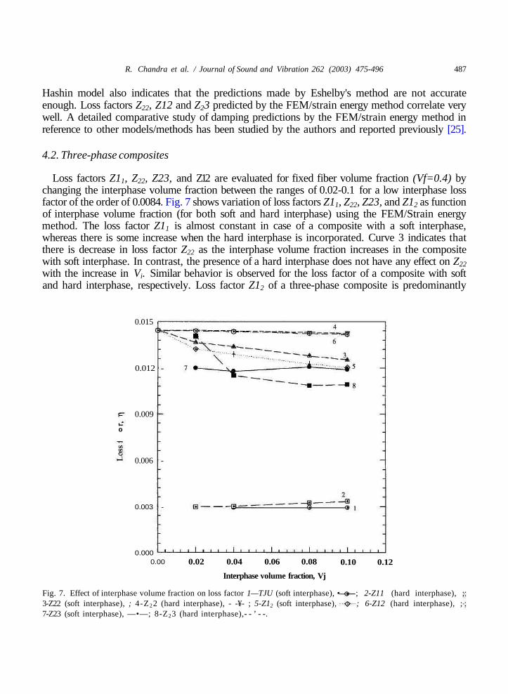
Loss factors Z11, Z22, Z23, and Z12 are evaluated for fixed fiber volume fraction (Vf=0.4) bychanging the interphase volume fraction between the ranges of 0.02-0.1 for a low interphase lossfactor of the order of 0.0084. Fig. 7 shows variation of loss factors Z11, Z22, Z23, and Z12 as functionof interphase volume fraction (for both soft and hard interphase) using the FEM/Strain energymethod. The loss factor Z11 is almost constant in case of a composite with a soft interphase,whereas there is some increase when the hard interphase is incorporated. Curve 3 indicates thatthere is decrease in loss factor Z22 as the interphase volume fraction increases in the compositewith soft interphase. In contrast, the presence of a hard interphase does not have any effect on Z22
with the increase in Vi. Similar behavior is observed for the loss factor of a composite with softand hard interphase, respectively. Loss factor Z12 of a three-phase composite is predominantly
o
0.015
0.012 -
0.009
0.006 -
0.003 -
0.0000.00 0.02 0.04 0.06 0.08
Interphase volume fraction, Vj
0.10 0.12
Fig. 7. Effect of interphase volume fraction on loss factor 1—TJU (soft interphase), •3-Z22 (soft interphase), ; 4-Z22 (hard interphase), - -¥- ; 5-Z12 (soft interphase),7-Z23 (soft interphase), —•—; 8-Z23 (hard interphase),- - ’ - -.
; 2-Z11 (hard interphase), ;; 6-Z12 (hard interphase), ;

488 R. Chandra et al. / Journal of Sound and Vibration 262 (2003) 475-496
0.020
0.016
0.012
0.008
0.004
nnnn
'-
_
: ripoa _^^
r a j " A ^,=0.02 to 0.002
—a
0.00 0.02 0.04 0.06 0.08 0.10 0.12Interphase volume fraction, V;
Fig. 8. Variation of loss factor Z11 as a function of Vi (3-D FEM model with soft interphase).
0.04 0.06 0.08 0.10 0.12
Interphase volume fraction Vj
Fig. 9. Variation of loss factor Z22 as a function of Vi (3-D FEM model with soft interphase).
dependent upon the status of the interphase, which is clear from curves 6-7. It is observed that Z12
for a composite with a soft interphase decreases appreciably with increase in Vi as compared tothe case of a hard interphase. A marginal reduction in Z12 with a hard interphase is due to minorvariation in the strain energy component of the interfacial region. It may be noted that the over allloss factor of composite from the FEM model is dependent on assumed values of interphaseproperties, i.e., loss factor and elastic modulus. A gradual decrease in the value of Z23 is predictedwith increasing Vi in case of a composite with a hard interphase (curve 8) whereas there is veryminor change in its value in case of a soft interphase (curve 7). Further details concerning thepercentage contribution of individual constituents, i.e., fiber, matrix and interphase, to the overallloss factor of the fiber-reinforced composite are given by Chandra et al. [26].
R. Chandra et al. / Journal of Sound and Vibration 262 (2003) 475-496
0.25
489
0.000.00 0.02 0.04 0.06 0.08 0.10 0.12
Interphase volume fraction, V;
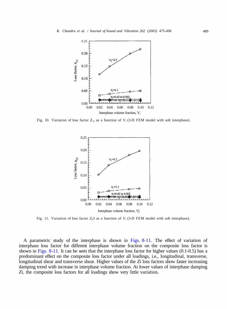
Fig. 10. Variation of loss factor Z12 as a function of Vi (3-D FEM model with soft interphase).
0.25
0.20 -
0.15 -
0.10 -
0.05 -
0.000.00 0.02 0.04 0.06 0.08 0.10 0.12
Interphase volume fraction, Vj
Fig. 11. Variation of loss factor Z23 as a function of Vi (3-D FEM model with soft interphase).
A parametric study of the interphase is shown in Figs. 8-11. The effect of variation ofinterphase loss factor for different interphase volume fraction on the composite loss factor isshown in Figs. 8-11. It can be seen that the interphase loss factor for higher values (0.1-0.5) has apredominant effect on the composite loss factor under all loadings, i.e., longitudinal, transverse,longitudinal shear and transverse shear. Higher values of the Zi loss factors show faster increasingdamping trend with increase in interphase volume fraction. At lower values of interphase dampingZi, the composite loss factors for all loadings show very little variation.
490 R. Chandra et al. / Journal of Sound and Vibration 262 (2003) 475-496
0.020
oH 0.015
0.014
(a)
0 30 60 90 120 150Orientation of gap, 6 (b)
30 60 90 120 150
Orientation of gap, 9180
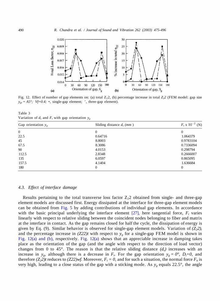
Fig. 12. Effect of number of gap elements on: (a) total Z22, (b) percentage increase in total Z22 (FEM model: gap sizeygs = A5°; Vf=0.4; •, single-gap element; ’, three-gap element).
Table 3Variation of ds and Ft with gap orientation yg
Gap orientation yg Sliding distance ds (mm ) Ft x (N)
022.54567.590112.5135157.5180
00.647168.80038.30864.01532.83486.05974.14040
01.0643790.97831040.73360940.2987940.26660070.8650951.6366840
4.3. Effect of interface damage
Results pertaining to the total transverse loss factor Z22 obtained from single- and three-gapelement models are discussed first. Energy dissipated at the interface for three-gap element modelscan be obtained from Fig. 5 by adding contributions of individual gap elements. In accordancewith the basic principal underlying the interface element [27], here tangential force, Ft varieslinearly with respect to relative sliding between the coincident nodes belonging to fiber and matrixat the interface in contact. As the gap remains closed for half the cycle, the dissipation of energy isgiven by Eq. (9). Similar behavior is observed for single-gap element models. Variation of (Z22)t
and the percentage increase in (Z22)t with respect to yg for a single-gap FEM model is shown inFig. 12(a) and (b), respectively. Fig. 12(a) shows that an appreciable increase in damping takesplace as the orientation of the gap (and the angle with respect to the direction of load vector)changes from 0 to 45°. The reason is that the relative sliding distance (ds) increases with anincrease in yg, although there is a decrease in Ft. For the gap orientation yg = 0°, Di=0, andtherefore (Z22)t reduces to (Z22)wf. Moreover, Ft = 0, and for such a situation, the normal force Fn isvery high, leading to a close status of the gap with a sticking mode. As yg equals 22.5°, the angle

R. Chandra et al. / Journal of Sound and Vibration 262 (2003) 475-496 491
0.00
(a)
0 30 60 90 120 150 180
Orientation of gap, 60 30 60 90 120 150 180
(b) Orientation of gap, 8
Fig. 13. Variation of energy dissipated by gap under (a) transverse, (b) transverse shear loading (FEM model: gap sizeygs = A5°; Vf=0.4; —•—, single-gap element; — ’ — , three-gap element).
between the average load vector and the gap direction becomes 22.5°. Table 3 shows the slidingdistance (ds) and Ft, for different values of yg, which have a direct bearing on the value of Di. Itcan be seen that although Ft decreases marginally with yg, the magnitude of ds increases, leadingto larger dissipation of energy at the interface. This is true up to yg = 45Q. Further, for45° ^0 0^9O°, there is a continuous decrease in Ft and ds. The following ratio gives a quantitativeidea; for example, (Ft)y = 67.5o/(Ft)e = 45o = 0.75 and (Ft)y = 90o/(Ft)e = 45o = 0.30, whereas (ds)y = 67.5°/(ds)y = 45° = 0.94 and (ds)y = 9o°/05Q<9 = 45o = 0.46. Thus, under the combined effects of Ft and (ds),(Z22)t decreases for 45°<09<9O°.
There is a slight increase in (Z22)t for yg = 112.5°. Thereafter, similar behavior for (Z22)t isrepeated for 112.5° p yg p 180° with a maximum at yg = 157.5°. Once again at yg = 180°, directionof load vector and gap direction coincide, leading to Di=0 and thus reducing to (Z22)t
= ( Z22) wf.The variation of Di vs yg for single-gap element models is shown in Fig. 13(a). A sharp increase inthe value of Di is clearly seen for yg in the region of about 45° and 157.5°, which explains the factthat (Z22)t attains the peak values at these angles. Fig. 12(b) shows the percentage increase in (Z22)tas a function of yg. Its pattern of variation is exactly similar to (Z22)t. It has an increasing trend for0°^9g^45°, followed by a reducing trend for 45° ^9g^67.5°. An increasing trend is againobservedfor 112.5°<09<157.5°. Similar behavior is observed for 18O°<09<36O° (the results arenot presented here) due to the geometric symmetry of the model.
Figs. 12(a) and (b) also show (Z22)t and the percentage increase in (Z22)t for models with three-gap elements with respect to yg. The behavior of (Z22)t and % increase in (Z22)t is similar to the onefor models with a single-gap element. This is also clear from the comparison of energy dissipatedper cycle for the two types of models in transverse loading as shown in Fig. 13(a). The reason forhigher Dh say for yg = 0°, is due to the contribution of gap elements having a gap orientationyg= +11.25° with respect to the gap axis. Similarly, Figs. 12(a) and (b) show that the peak valueof (Z22)t and the percentage increase in (Z22)t correspond to yg = 45° and 157.5° as in case of single-gap element models. However, their magnitudes are on the higher side. The percentage increase in(Z22)t for a single-gap element is 23.75 whereas for the three-gap element model, it is 27.8 atyg = 45°. Corresponding to the other peak, i.e., at yg= 157.5°, the value of the percentage increasein (Z22)t is 18.85 and 25.08, respectively, for the single-gap element and three-gap element models.

492 R. Chandra et al. / Journal of Sound and Vibration 262 (2003) 475-496
0.021
0.020
oH 0.015
0.014
(a)
0 30 60 90 120 150 180
Gap orientation axis, 9 (b)
0 30 60 90 120 150 180
Orientation of gap axis, 8,
Fig. 14. Effect of number of gap elements on: (a) total Z23, (b) percentage increase in total Z22 (FEM model: gap sizeygs = 45°; Vf=0.4; • , single-gap element; ’, three-gap element).
ET*
or,
tact
loss
tal.
o
U.UiU
0.016
0.012
0.008
0.004
nnnn
_
-
-
.a
(a)
0.0 0.2 0.4 0.6 0.8 1.0
Relative position of gap, x/1 (b)
0.0 0.2 0.4 0.6 0.8 1.0
Relative position of gap, x/1
Fig. 15. Effect of location of gap on (a) total Z12 and (b) percentage increase in total Z12 (FEM model: inplane shearloading; no. of gap elements = 1; gap size = 23.76 mm; Vf=0.4).
The comparison of the results shows a marginal difference in value of percentage increase in (Z22)tfor yg = 45°(~4%) and yg= 157.5°(~6%). This shows consistency of results obtained, indicatingthat the number of gap elements to model discontinuity does affect the loss factor values onlymarginally. An optimum selection of the number of gap elements for the same gap size gives betterresults. The direction of the load with respect to orientation of the gap axis has a greater effect on(Z22)t and on the percentage increase in (Z22)t. If the orientation of the gap axis coincides with theload vector, there is no effect of slip at the interface on (Z22)t, and (Z22)t = (Z22)wf.
Variation of energy dissipation in transverse shear loading from single- and three-gap elementmodels corresponding to the orientation of the gap axis is plotted in Fig. 13(b). Here also it can beseen that variation of A for both single- and three-gap element models are closely related. It maybe noted that the use of three-gap elements is primarily to test its adequacy over the single-gapelement. Figs. 14(a) and (b) show the variation of (Z23)t and the percentage increase in (Z23)t as afunction of yg, respectively. Thus, a close relationship is observed for (Z23)t in both the modelswith a maximum at yg= 135°. The total loss factor is somewhat higher in case of the three-gap

R. Chandra et al. / Journal of Sound and Vibration 262 (2003) 475-496 493
0.005 -
0.0020.0 0.2 0.4 0.6 0.8 1.0
(a) R e l a t i v e p o s i t i o n o f g a p , x / 1
60
50
sf 40
30
2 0
10
(b)
00.0 0.2 0.4 0.6 0.8 1.0
Relative position of gap, x /1
Fig. 16. Effect of location of gap on (a) total Z11 and (b) percentage increase in total Z11 (FEM model: longitudinalloading; no. of gap elements = 1; gap size = 23.76 mm; Vf=0.4).
element model as compared to the single-gap element model. The percentage increase in (Z23)t atyg= 135° is 34.84 (single-gap model) and 40.8 (three-gap element) for the two type of models.
Figs. 15(a) and (b) show the effect of location of the gap along the axis at the interface on (Z12)tand the percentage increase in (Z12)t. It can be seen that (Z12)t is almost independent of the relativeposition of the gap element (x/l) along the fiber length so far as the discontinuity is within thestructure (0ox / lo 1). However, for the discontinuity starting at the edge, i.e., x/l = 1, the value of(Z12)t increases slightly to 1.6 x 1CT2. Similarly, the percentage increase in (Z12)t for thediscontinuity of the same size within the composite, is constant and independent of the relativeposition of the gap element up to 0.075px/lp0.925. However, for a discontinuity at the edge, i.e.,x/l= 1, there is a sudden rise in the percentage increase in (Z12)t, of the order of 6.25. This indicatesthat the effect of debonding or discontinuity at the interface on (Z12)t is more predominant at theedges. When the damage is away from the edges along the fiber matrix, (Z12)t D Z12 of the pristinematerial.
Figs. 16(a) and (b) show variation of (Z11)t and percentage increase in (Z11)t with the relativeposition of the gap along the fiber-matrix interface. It can be observed that there is an increase inZ11)t in reference to pristine material due to slip at the fiber-matrix interface for the same gap size.However, it is independent of x/l for 0 o x / l o 1, when the debonding is within the composite. Thetotal loss factor (Z11)t increases sharply to 5.088 x 10~3 for debonding starting from the edge.Similarly, the percentage increase in (Z11)t is fairly constant (B9.4%) for 0.075 p x / l p 0.925,whereas at the edge (x/l), it jumps to 56%. Thus, the sensitivity of longitudinal loading on (Z11)and the percentage increase in (Z11) is indicated through these results.
5. Conclusions
An integrated FEM/Strain energy approach has been worked out to predict loss factors (Z11,Z22, Z23, and Z12) for two-phase, three-phase composites with damage (interfacial discontinuity).The following conclusions have been made.

494 R. Chandra et al. / Journal of Sound and Vibration 262 (2003) 475-496
5.1. Two-phase composites
Comparison of damping predictions for two-phase (fiber-matrix) composites are madebased on several models and has shown that the finite element/strain energy model baseddamping results presented here are best for a single representative volume element. Thus,the loss factors are higher for all loading conditions due to the reason that only the actualstate of stress is accounted for. There is better correlation of the loss factor predictionsmade by Eshelby's method, and the Hashin's model, and the Halpin-Tsai and Tsaimodel. The only exception is the case of the longitudinal loss factor (Z11), where deviationis observed in the prediction based on Eshelby's method. The other methods give betterresults.
Loss factors predicted through the unified micromechanics approach do not compare well withother methods. Consideration of variable stress (in the FEM method) and the additional effect offiber-to-fiber interaction (in Eshelby's method) render results from these theories rather moreaccurate.
5.2. Three-phase composites
Damping coefficients for fiber-reinforced composites with hard and soft interphases inlongitudinal, transverse, longitudinal and transverse shear loading conditions predicted usingthe FEM/Strain energy approach employing both the 2D and 3D FEM models provide theunderstanding as to how damping is related to the modulus and the volume fraction of theinterphase. The results provide an insight into the interplay and relative contributions of the threeconstituents, i.e., the fiber, matrix and interphase, to various damping loss factors. The change inproperties of fiber, matrix and interphase will lead to a change in the magnitude of effectiveness ofthe interphase, but the manner in which the interphase would affect the various loss factorsdepends predominately upon whether the hard or soft interphase is chosen. Loss factor of fiber-reinforced composites can be improved to a great extent by incorporating highly dampedinterphases.
5.3. Effect of interface damage
The damage in composite is modelled as a discontinuity at the fiber-matrix interface(debonding) by a 2-D gap element using the finite element method to predict transverse,transverse shear, longitudinal and longitudinal shear loss factors. It is observed that the dampingis sensitive to damage and its orientation with respect to the loading directions. The transverseloss factor is maximum when the orientation of discontinuity (angle of orientation of gap) is 45°or 157.5° whereas the transverse shear loss factor has a maximum value for 135° gap orientation.Both longitudinal and shear loss moduli are independent of the location of the discontinuity alongthe axis of a fiber as far as it is within the composite. The percentage increase in damping isappreciable if the discontinuity is at the edge (approximately 50% for longitudinal load and 6%for longitudinal shear).
R. Chandra et al. / Journal of Sound and Vibration 262 (2003) 475-496 495
Appendix A. Nomenclature
and
ntotalWf,Wi ,Wand Wc
Wid
s, eFt and Fn
,Wm
DDid
Vf, Vi and Vm
GWygs
Nf and Nm
xI
loss factors in longitudinal, transverse, longitudinal and transverse shear, resp.
loss factor of compositeloss factor without the consideration of friction at the interfacetotal loss factor of the compositestrain energy in fiber, interphase, matrix and composite, resp.
total strain energy with interfacial discontinuitystress and straintangential normal forces, resp.coefficient of frictionapplied forceforce amplitude of applied forcerelative displacement between the nodes of the friction elementenergy dissipated at the fiber-matrix interfaceenergy dissipation due to individual discontinuity at interfacetotal thickness of the interphasevolume fraction of fiber, interphase and matrix, resp.gap widthgap sizegap orientationnumber of fiber elements in fiber and matrix, resp.friction or gap element numberlocation of gap element along the fiber axislength of the model along the fiber axis
References
[1] P. Zioniev, Y.N. Ermakov, Energy Dissipation in Composite Materials, Technomic Publication, Lancaster, PA,1994.
[2] R.F. Gibson, S.J. Hwang, H. Kwak, Micromechanical modelling of damping in composites including interphaseeffects, Proceedings of 36th International SAMPE Symposium, Society for the Advancement of Material andProcess Engineering, Covina, Vol. 1, 1991, pp. 592-606.
[3] D.J. Nelson, J.W. Hancock, Interfacial slip and damping in fiber-reinforced composites, Journal of MaterialScience 13 (1978) 2429-2440.
[4] J.M. Kenny, M. Marchetti, Elasto-plastic behavior of thermoplastic composite laminates under cyclic loading,Composite Structures 32 (1995) 375-382.
[5] S. Chang, C.W. Bert, Analysis of damping for filamentary composite materials, Proceedings of Sixth St. LouisSymposium, American Society of Metals, 1973, pp. 51-62.
[6] L.B. Crema, A. Castellani, U. Drago, Damping characteristics of fabric and laminated kevlar composites,Composites 20 (6) (1989) 593-596.
[7] D.A. Saravanos, C.C. Chamis, Unified micromechanics of damping for unidirectional and off axis fibercomposites, Journal of Composite Technology and Research 12 (1990) 31-40.

496 R. Chandra et al. / Journal of Sound and Vibration 262 (2003) 475-496
[8] D.A. Saravanos, C.C. Chamis, An integrated methodology for optimizing the passive damping of compositestructures, Polymer Composites 11 (6) (1990) 328-336.
[9] M. Kaliske, H. Rther, Damping characterization of unidirectional fiber-reinforced composites, CompositeEngineering 5 (5) (1995) 551-567.
[10] R. Chandra, S.P. Singh, K. Gupta, FEM modelling for damping evaluation of fiber-reinforced composites,Proceedings of National Symposium on Dynamics, NASDYN 98, Indian Institute of Technology, Madras, India,1998, pp. 109-114.
[11] R. Chandra, S.P. Singh, K. Gupta, Comparative study of damping models for fiber- reinforced composites,Proceedings of 11th ISME Conference on Mechanical Engineering, Indian Institute of Technology, Delhi, India,1999, pp. 489-495.
[12] S.K. Chaturvedi, G.Y. Tzeng, Micromehanical modelling of material damping in discontinuous fiber three-phasepolymer composites, Composite Engineering 1 (1) (1991) 49-60.
[13] J. Vantomme, A parametric study of material damping in fiber-reinforced plastics, Composites 26 (1995) 147-153.[14] I.C. Finegan, R.F. Gibson, Improvement of damping at micromechanical level in polymer composite materials
under transverse loading by the use of special fibre coatings, Journal of Vibrations and Acoustics 120 (1998)623-627.
[15] R. Chandra, Some Micromechanical Studies on Damping in Fiber-Reinforced Composites, Ph.D Thesis,Department of Mechanical Engineering, Indian Institute of Technology, Delhi, India, 1999.
[16] R. Chandra, S.P. Singh, K. Gupta, Damping studies in fiber-reinforced composites—a review, CompositeStructures 46 (1) (1999) 41-51.
[17] R. Chandra, A.K. Mallik, R. Praphakaran, Damping as a measure of damage in composites, Journal of TechnicalCouncil of ASCE (American Society of Civil Engineers) 108 (1982) 106-111.
[18] J.M. Curtis, D.R. Moore, Fatigue testing of multiangle laminates of CF/PEEK, Composites 19 (1988) 446-455.[19] E.E. Ungar, E.M. Kerwin Jr., Loss factor of viscoelastic systems in terms of energy concepts, Journal of Acoustical
Society of America 34 (1962) 954-958.[20] Z. Hashin, Analysis of properties of fiber composites with anisotropic heterogeneous materials, Journal of Applied
Mechanics 46 (1979) 543-550.[21] Y.H. Zhao, G.J. Weng, Effective elastic moduli of ribbon-reinforced composites, Transactions of American
Society of Mechanical Engineers 57 (1990) 158-167.[22] S.W. Tsai, Structural behavior of composites materials, NSA-CR-71, July 1964.[23] J.C. Haplin, S.W. Tsai, Effect of environmental factors on composite materials, AFML-TR, 67-423, June 1969.[24] JD. Eshelby, The determination of the elastic field of an elliptical inclusion and related problems, Proceedings of
the Royal Society, London, 1957, pp. 376-396.[25] R. Chandra, S.P. Singh, K. Gupta, Micromechanical damping models for fiber-reinforced composites: a
comparative study, Composites Part A: Applied Science and Manufacturing 33 (2002) 787-796.[26] R. Chandra, S.P. Singh, K. Gupta, Studies on prediction of damping in three-phase fiber-reinforced composites: a
FEM approach, Defence Science Journal, in press.[27] V. Tvergaard, Effect of fiber debonding in whisker reinforced metal, Material Science Engineering A 125 (1990)
203-213.