NAS-A TECHNICAL NASATR R-421REPORT

(NASA-TB-R-421) . A STUDY OF THE N74-14741NONLINEAR AERODYNAMICS OF BODIES INNONPLANAR NOTION Ph.D. Thesis -Stanford Univ., Calif. (NASA) -94 p LC Unclas$3.75 , CSCL 01A 81/01 26735

A STUDY OF THE NONLINEAR AERODYNAMICS"OF BODIES IN NONPLANAR MOTION

by Lewis Barry Schiff

Ames Research Center

Moffett Field, Calif 94035

NATIONAL AERONAUTICS AND SPACE ADMINISTRATION * WASHINGTON, D. C. * JANUARY 1974

1. Report No. 2. Government Accession No. 3. Recipient's Catalog No.TR-421

4. Title and Subtitle 5. Report Date

A Study of the Nonlinear Aerodynamics of Bodies in Nonplanar January 1974

Motion 6. Performing Organization Code

7. Author(s) 8. Performing Organization Report No.

Lewis Barry Schiff A-5057

10. Work Unit No.

9. Performing Organization Name and Address 501-06-01-23Ames Research Center, Moffett Field, Calif. 94035 andStanford University, Stanford, Calif. 11. Contract or Grant No.

13. Type of Report and Period Covered

12. Sponsoring Agency Name and Address Technical Report

National Aeronautics and Space Administration 14. Sponsoring Agency CodeWashington, D.C. 20546

15. Supplementary Notes

Submitted to Stanford University as partial fulfillment of Ph.D. degree, August 1973.

16. AbstractConcepts from the theory of functionals are used to develop nonlinear formulations of the

aerodynamic force and moment systems acting on bodies in large-amplitude, arbitrary motions. Theanalysis, which proceeds formally once the functional dependence of the aerodynamic reactions uponthe motion variables is established, ensures the inclusion, within the resulting formulation, ofpertinent aerodynamic terms that normally are excluded in the classical treatment. Applied to thelarge-amplitude, slowly varying, nonplanar motion of a body, the formulation suggests that the aero-dynamic moment can be compounded of the moments acting on the body in four basic motions: steadyangle of attack, pitch oscillations, either roll or yaw oscillations, and coning motion. Coning,where the nose of the body describes a circle, around the velocity vector, characterizes the non-planar nature of the general motion.

With the above motivation, a numerical finite-difference technique is develooed for computingthe inviscid flow field surrounding a body in coning motion in a supersonic stream. Computationscarried out for circular cones in coning motion both at low supersonic and hypersonic Mach numbersconfirm the adequacy of a linear moment formulation at low angles of attack. At larger angles ofattack, however, the forces and moments become nonlinear functions of the angle of attack. Compu-tational results for the reactions on the circular cone at the higher angles of attack agree wellwith experimental measurements within the range of variables investigated.. This indicates that theinitial nonlinear behavior of the aerodynamic forces and moments is governed primarily by the

inviscid flow.

17. Key Words (Suggested by Author(s)) 18. Distribution StatementNonlinear aerodynamics

Nonsteady aerodynamics I Unclassified

Nonplanar motionSupersonic aerodynamics

Large angles of attack

19. Security Classif. (of this report) 20. Security Classif. (of this page) 21. No. of Pages 22. Price*Domestic, $3.75

Unclassified Unclassified 93 Foreign, $6.25

*For sale by the National Technical Information Service, Springfield, Virginia 22151

TABLE OF CONTENTS

Page

NOMENCLATURE . . . . . . . . . . . .. .. . . . . . . .. . . . . v

SUMMARY . . . . . . . . . . .. . .. . .. .. ........ . . . .. .. 1

1. INTRODUCTION . . . . . . . . . . . . . . . . ..... . ... . . . 2

2. NONLINEAR FORMULATION - REVIEW AND EXTENSION . . . . . . . . . 6

2.1 Coordinate Systems . . . . . . . . . . . . . . . . . ..... 7

2.2 Development for Planar Motion . ..... .. ...... 12

2.2.1 Concept of a Functional . . . . . . . . . . . . . . 12

2.2.2 Nonlinear Indicial Response . . . . . . . . . . . . 13

2.2.3 Approximate Formulation for Slowly VaryingMotions . . . . . . . . . . . ... . . . . . . . . 15

2.2.4 Extensions to Describe More General Motions . . . . 19

2.3 Development for General Body in Free Flight . . . . . . . 21

2.3.1 Body-Fixed Axes . .... . . . . . . . . . . . . . 22

2.3.2 Aerodynamic Axes . . . . . . . . . . . . . . . . . 25

2.3.3 Correspondence Between Axis Systems . . . . . . . . 27

2.3.4 Bodies of Revolution . . . . . . . . . . . . . . . 28

2.3.5 Potential Application to Airplane Spins . . . . . . 31

3. NUTIRICAL FLOW-FIELD SOLUTION . . . . . . . . . . . . . . . . . 32

3.1 Method of Solution . .... . . . . . . . . . . . ... 34

3.2 Gasdynamic Equations . . . . . . . . . . ... ..... . . . . 35

3.3 Differencing Scheme . . . . .............. .. . . . . . . . . . . 39

3.4 Boundary Conditions . . . . . . . . . . . . . . .. . . . 42

3.5 Initial Solution . . . . . . . . . . . . . . . . . . . . . 44

3.6 Results . . . . . . . . . . . . . . . . . . ...... . 46

3.6.1 100 Circular Cone at M = 2; Nonlinear vs. ViscousEffects . . .. . . .. . . . . . . . . . . . . . 46

iii

Page

3.6.1.1 Flow-Field Results . . . . . . . . ... 47

3.6.1.2 Force and Moment Coefficients . ..... 51

3.6.2 100 Circular Cone at M = 10 . . . . . . . . . . . 54

3.6.3 Elliptic Cone at M = 2 . ............. 55

3.6.3.1 Normal-Force Coefficient . ........ 55

3.6.3.2 Side-Moment Coefficient . ........ 55

4. CONCLUDING REMARKS . .. . . . . . . . . . . . . . ... . . .. 57

APPENDIX A . . . . . . . . . . . . . . . . . . . . . . . . . . . . 58

REFERENCES . . . . . . . . . . . . . . . . . . . . . . . . . . . . 61

FIGURES . . . . . . . . . . . . . . . . . . . . . . . . . . . . . . 65

iv

NOMENCLATURE

Cy side-force coefficient in the aerodynamic axis system (along

y), 2(side force)/p V2S

CZ normal-force coefficient in the aerodynamic axis system

(along z), 2(normal force)/poV 2S

CyC Z side-force and normal-force coefficients in the body-axis

system; along yB,zB, respectively

C rolling-moment coefficient in the aerodynamic axis system

(along xB), 2L/poV 2Sk

Cm pitching-moment coefficient in the aerodynamic axis system

(along y), 22/poV 2SZ

C side-moment coefficient in the aerodynamic axis system

(along z), 2N/poV 2 SZ

C, mC n rolling-, pitching-, and yawing-moment coefficients in the

body-axis system; along xBYB,zB, respectively

h total enthalpy

L,I,N moment components along the xB,y,z aerodynamic axes,

respectively

ecg distance from center of gravity to nose of body (-sti p )

z reference length (body length, (s fina- stip))

p pressure

pBq Br B components along the xBYB,zB axes, respectively, of the

total angular velocity of the body axes relative to

inertial space

q,r components of the total angular velocity along the y,z

aerodynamic axes, respectively, Eq. (2.6)

S reference area (body base area)

v

s,T,O computational axes, origin at center of gravity, s positive

in the negative xB direction, T and 8 polar coordinates

in planes normal to s, Fig. 1

t time

B',vB,B components of flight velocity along xBYB,zB axes, respec-

tively, Fig. 1

u,v,w components of local flow velocity in the s,T,6 directions,

respectively

V flight velocity

xBYBZ B body-fixed axes, origin at center of gravity, xB coincident

with a longitudinal axis of the body, Fig. 1

xB,y,z aerodynamic axes, origin at center of gravity, xB,z in the

plane of the resultant angle of attack, y in the cross-

flow plane normal to the resultant angle-of-attack plane,

Fig. 1

a, angle of attack and sideslip in body axes, respectively,

Eq. (2.7)

a angle-of-attack parameter in body-axis system, wB/V

f angle-of-sideslip parameter in body-axis system, vB/V

Y dimensionless axial component of flight velocity (along xB),

Fig. 1 and Eq. (2.2)

Y ratio of specific heats

6 magnitude of the dimensionless crossflow flight velocity in

the aerodynamic axis system, Fig. 1 and Eq. (2.2)

transformed circumferential independent coordinate, Eq. (3.6)

transformed radial independent coordinate, Eq. (3.6)

P local flow mass density

Po atmospheric mass density

vi

0 resultant angle of attack defined by xB axis and flight

velocity vector, Fig. 1

centrifugal potential, Eq. (3.3)

< coning rate of xB axis about the flight velocity vector,

Fig. 1 (for body in coning motion, total angular velocity

of body-fixed axes with respect to inertial space)

Sangular inclination of the zB axis from the z axis in the

crossflow plane, Fig. 1

w1 ,w2 ,w3 components of total angular velocity in the s,T,8 directions,

respectively

dt

vii

A STUDY OF THE NONLINEAR AERODYNAMICS OF BODIES

IN NONPLANAR MOTION*

Lewis Barry Schiff

Ames Research Center

SUMMARY

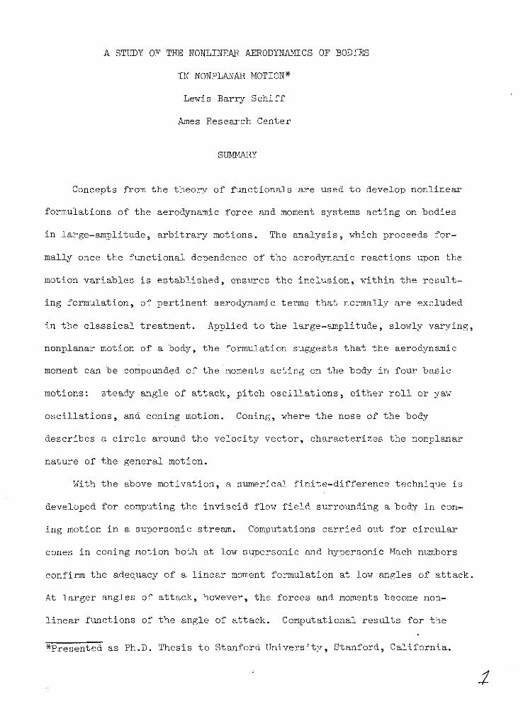
Concepts from the theory of functionals are used to develop nonlinear

formulations of the aerodynamic force and moment systems acting on bodies

in large-amplitude, arbitrary motions. The analysis, which proceeds for-

mally once the functional dependence of the aerodynamic reactions upon the

motion variables is established, ensures the inclusion, within the result-

ing formulation, of pertinent aerodynamic terms that normally are excluded

in the classical treatment. Applied to the large-amplitude, slowly varying,

nonplanar motion of a body, the formulation suggests that the aerodynamic

moment can be compounded of the moments acting on the body in four basic

motions: steady angle of attack, pitch oscillations, either roll or yaw

oscillations, and coning motion. Coning, where the nose of the body

describes a circle around the velocity vector, characterizes the nonplanar

nature of the general motion.

With the above motivation, a numerical finite-difference technique is

developed for computing the inviscid flow field surrounding a body in con-

ing motion in a supersonic stream. Computations carried out for circular

cones in coning motion both at low supersonic and hypersonic Mach numbers

confirm the adequacy of a linear moment formulation at low angles of attack.

At larger angles of attack, however, the forces and moments become non-

linear functions of the angle of attack. Computational results for the

*Presented as Ph.D. Thesis to Stanford University, Stanford, California.

reactions on the circular cone at the higher angles of attack agree well

with experimental measurements within the range of variables investigated.

This indicates that the initial nonlinear behavior of the aerodynamic

forces and moments is governed primarily by the inviscid flow.

1. INTRODUCTION

Linear formulations of the aerodynamic force and moment systems do not

properly describe the aerodynamic reactions on flight vehicles in nonplanar

motions at large resultant angles of attack. As a result, equations of

vehicle motion incorporating linear aerodynamic formulations have often

failed to correctly predict the variety of motion such flight vehicles can

experience. In the past this has been a problem primarily associated with

the flight of slender bodies of revolution. However, the requirements for

increased angle-of-attack ranges for proposed high performance aircraft and

space shuttle vehicles, as well as those envisioned for STOL aircraft, have

tended to make the deficiencies of the linear formulation a problem of more

widespread concern in the analysis of vehicle motions.

In the linear formulation, a reference flight condition is chosen,

for example, the steady level flight of an airplane, and the deviations of

the angular orientation and angular velocities of the body are measured

from the reference state. The aerodynamic reactions are expressed in a

Taylor series expansion in terms of the deviations and only terms linear

in the disturbance quantities are retained. The coefficients of the expan-

sion are called the aerodynamic derivatives and are evaluated at the refer-

ence state. When applied to a combined pitching and yawing motion, the

linear formulation can be shown to be equivalent to the vector decomposition

of the nonplanar motion into two orthogonal planar motions, to the subsequent

2

treatment of each planar motion as if the other were absent, and to the

superposition of the results. This approach has had a great deal of suc-

cess, particularly for the case of airplane motions where the deviations

from the reference state are small. A rather complete treatment of the

linear formulation has been presented by Etkin.1 At large resultant angles

of attack, however, it is physically clear that the reactions due to

motion in one plane will be influenced by the presence of the other motion,

and thus a more precise formulation will be necessary to account for this

coupling.

The form that extensions of the linear formulation should take to

account for the large angular deviations from the reference state has not

yet been settled. Guided by the fact that the static forces acting on a

body of revolution lie in the plane of the resultant angle of attack,

Nicolaides et al. 2 and Ingram, 3 concerned with missile aerodynamics,

assumed that the form of the nonlinear generalization for a body of revo-

lution was the same as that of the linear formulation, but that the aero-

dynamic derivatives were nonlinear functions of the magnitude of the

resultant angle of attack. If this formulation is applied to the combined

pitching and yawing motions of a nonspinning axisymmetric body, it predicts

that the aerodynamic damping in the plane of the resultant angle of attack

is equal to that acting perpendicularly to the angle-of-attack plane. It

can be shown by a comparison of the experimental results of Iyengar4 with

those of Schiff and Tobak5 that this is untrue for such bodies at large

angles of attack. Murphy 6 proposed an extension of the linear formulation

which allowed for the possibility of unequal aerodynamic dampings in and

normal to the angle-of-attack plane. Unlike the previous one, Murphy's

formulation is therefore capable of correctly distinguishing between the

out-of-plane damping and the out-of-plane classical Magnus forces in the

case of the nonplanar motion of a spinning body of revolution.

Another approach has been developed by Tobak et al.,7 -10 who used con-

cepts from nonlinear functional analysis to develop a formulation of the

aerodynamic force and moment system for an arbitrarily shaped body that

does not depend on a linearity assumption. This formulation has been shown

to be equivalent to that of Murphy for the special case of a body of revo-

lution, 9 and reduces to the form of the linear formulation for small resul-

tant angles of attack. The formulation suggests that the aerodynamic reac-

tions on a body in an arbitrary nonplanar motion can be compounded of the

forces and moments acting on the body in four characteristic motions, three

of which are well known. The fourth, coning motion, in which the nose of

the body describes a circle around the velocity vector, is seen to have

particular significance since the nonlinear behavior, with increasing angle

of attack, of the contribution to the total force and moment due to coning

motion cannot be evaluated from the contributions due to any planar motions.

Experimental evaluations5, 8 of the contribution due to the coning of a body

of revolution have confirmed this and have shown this contribution to be a

potential cause of circular limit motions at large resultant angles of

attack. In addition, it is anticipated that the contribution due to con-

ing motion will be important in correctly describing the pre- and post-

stall behavior of aircraft-like bodies at large angles of attack.

The objectives of the present work are twofold. The first is to

review and unify the development of the nonlinear formulation proposed by

Tobak et aZ. and to remove from this analysis an unnecessary assumption of

constant flight speed. The second, and more important, objective is to

present a numerical method for computing the flow field surrounding a body

4

in coning motion in a supersonic stream. A finite-difference scheme of

MacCormack, 11 developed as a shock-capturing technique for computing com-

plex, steady, three-dimensional, inviscid flow fields by Kutler and

Lomax, 12 is extended to the case of coning motion. The capabilities and

limitations of the method are described. Results of computations for

slender conical bodies in coning motion at various supersonic Mach numbers

are presented and are compared with experimental results and with the

results of other analytical and numerical methods, where applicable. The

results will be seen to exhibit significant nonlinear behavior with

increasing resultant angle of attack, and the significance of the non-

linearities will be discussed.

The author wishes to acknowledge and thank Professor Samuel McIntosh,

Jr., and Professor Holt Ashley for their advice and encouragement during

the course of this work. Grateful acknowledgment is also given to Murray

Tobak of the NASA Ames Research Center for his valuable advice and helpful

consultation, and to Susan Schiff for her encouragement and for her help

in preparing the manuscript.

Finally, acknowledgment is given to the National Aeronautics and

Space Administration for support of the research and of the author's

graduate study through the Honors Cooperative Program with Stanford

University.

2. NONLINEAR FORMULATION - REVIEW AND EXTENSION

In a series of papers, 7- 1 0 concepts from the theory of functionals

were used to develop a nonlinear formulation of the aerodynamic force and

moment system acting on a body performing motions of interest, the first

being the planar motion of an airplane at large angle of attack.7 The

analysis was extended to the large-amplitude, nonplanar angular motions of

a body of revolution whose mass center traversed a straight-line path,8

and showed that the total moment could be compounded of the contributions

from four simple motions. Further extensions of the analysis to the free

flight of a body of revolution 9 and of an arbitrarily shaped body1 0 showed

that even in these more general cases the total moment still could be

determined from the contributions from the same four simple motions. The

resulting formulation allows the angular deviations of the body to be

large, but is valid only for the low angular rates typical of aircraft

motions. Unfortunately, a uniform notation was not employed throughout

the series, while the assumptions of the analysis, covered in detail for

the planar case, were abbreviated in the later works. Additionally, it

was unnecessarily assumed that the flight speed remained constant over the

course of the motion considered. In this chapter the development of the

nonlinear moment system is reviewed for the large-amplitude planar motion

of an arbitrary body whose flight speed varies, and it is indicated how

the formulation can be extended to more accurately represent motions of

higher frequencies. The formulation is then developed for the most general

case, that of an arbitrarily shaped body in free flight, again removing the

restriction of constant flight speed. Finally, the resulting formulation

is specialized to the previously reported cases.

6

2.1 Coordinate Systems

Three axis systems having a common origin at the body's mass center,

and a common axis xB aligned with a longitudinal axis of the body, will

be used to describe the motion in all cases considered. Some latitude

exists in the choice of the longitudinal axis, and this freedom can be

used to simplify the description of a particular motion. For example,

when describing the motions of an airplane-like body, the xB axis is

usually chosen to be initially coincident with the direction of steady

flight. Alternatively, when describing the flight of a body of revolution,

the xB axis is most often, but not necessarily, chosen as the axis of

axial symmetry.

Axes xB, YB, zB are fixed to the moving body (Fig. 1). The compo-

nents of the flight velocity vector of magnitude V, resolved along the

xB, YB ZB body-fixed axes, are uB, vB, wB, respectively. Thus

V= u + v + W (2.1)

The resultant angle of attack a is defined by the flight velocity vector

and the xB axis. The plane formed by the yB' zB axes is the crossflow

plane, illustrated in Fig. l(a). The projection of a unit vector in the

flight velocity direction onto the crossflow plane is a vector with magni-

tude 6, and will be called the dimensionless crossflow velocity vector.

Reference to Fig. l(b) gives

6 = 2 = sin a (2.2a)

y = - = cos a (2.2b)

S-= tan a (2.2c)Y

The components of the angular velocity vector of the body relative to

inertial space, resolved along the XB, y, zB body axes, are pB' qB'

rB, respectively.

A second axis system, xB, y, , is chosen to be nonrolling with

respect to inertial space. Specifically, the component of the angular

velocity vector of the xB, y, z axes measured with respect to inertial

space, resolved along the xB axis, is zero, while the components

resolved along the y, z axes are q, r, respectively. The nonrolling

axis system has been used extensively in the field of missile aerodynamics,

since its use, together with the assumption of small angular deviations,

leads to closed-form solutions of the equation of vehicle motion. The

angle ; through which the body axes have rolled at any time t can be

defined relative to the nonrolling axis system as

=0 PB dT (2.3)

The angular inclination X of the crossflow velocity vector 6 is mea-

sured relative to the nonrolling axis system, while is the angular

inclination of the body axes from the crossflow velocity vector. With

the aid of Fig. l(a), the body roll rate is seen to be the sum

8

PB = + (2.4)

The components of the angular velocity of the body relative to inertial

space resolved in the nonrolling axis system, PB,' c r, are related to

those resolved in the body axis system, pB, aqB rB' through

+ ir = ei(q B + irB) (2.5)

Finally, axes XB, y, z will be called the aerodynamic axes. Axis

z lies in the crossflow plane and is coincident with the crossflow veloc-

ity vector; axis y lies in the crossflow plane normal to the direction

of 6. The components of the angular velocity of the body resolved in

the aerodynamic axis system, pB, q, r, are related to those resolved in

the body axes through

q + ir = ei(qB + irB) (2.6)

In accordance with Ref. 10, wB/V will be called the angle-of-attack

parameter &, and VB/V will be called the angle-of-sideslip parameter

3. They are related to the standard NASA definitions of angle of attack

a and angle of sideslip B through

tan a = = - (2.7a)uB '

sin = -B = (2.7b)

9

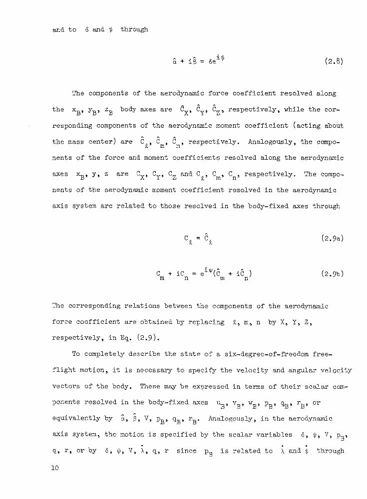
and to 6 and through

& + i0 = Se (2.8)

The components of the aerodynamic force coefficient resolved along

the xB, yB' zB body axes are OX, CY, CZ , respectively, while the cor-

responding components of the aerodynamic moment coefficient (acting about

the mass center) are C, Cm Cn, respectively. Analogously, the compo-

nents of the force and moment coefficients resolved along the aerodynamic

axes xB, y, z are CX, Cy, CZ and C , Cm, Cn, respectively. The compo-

nents of the aerodynamic moment coefficient resolved in the aerodynamic

axis system are related to those resolved in the body-fixed axes through

C = C (2.9a)

Cm +iC = e (C + i ) (2.9b)m n m n

The corresponding relations between the components of the aerodynamic

force coefficient are obtained by replacing Z, m, n by X, Y, Z,

respectively, in Eq. (2.9).

To completely describe the state of a six-degree-of-freedom free-

flight motion, it is necessary to specify the velocity and angular velocity

vectors of the body. These may be expressed in terms of their scalar com-

ponents resolved in the body-fixed axes uB' vB' WB9 PB' qB, rB, or

equivalently by , p, V, pB' qB rB. Analogously, in the aerodynamic

axis system, the motion is specified by the scalar variables 6, , V, pB'

q, r, or by 6, p, V, , q, r since pB is related to X and * through

10

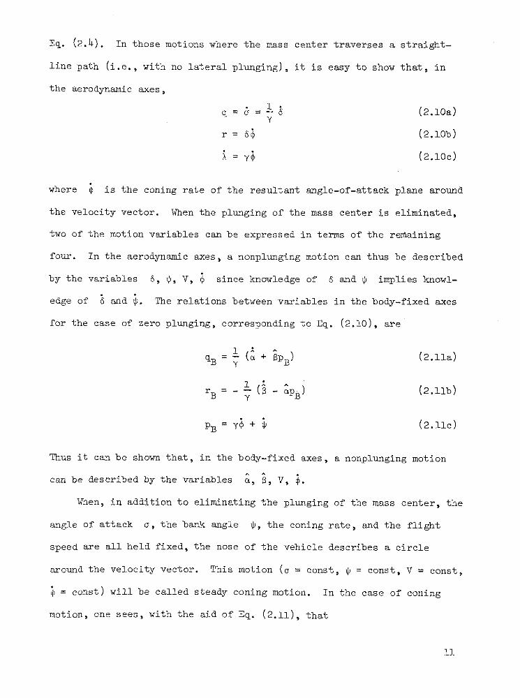
Eq. (2.4). In those motions where the mass center traverses a straight-

line path (i.e., with no lateral plunging), it is easy to show that, in

the aerodynamic axes,

q = (2.10a)Y

r = 65 (2.10b)

1 = ys (2.10c)

where $ is the coning rate of the resultant angle-of-attack plane around

the velocity vector. When the plunging of the mass center is eliminated,

two of the motion variables can be expressed in terms of the remaining

four. In the aerodynamic axes, a nonplunging motion can thus be described

by the variables 6, 4, V, $ since knowledge of 6 and 4 implies knowl-

edge of 6 and 4. The relations between variables in the body-fixed axes

for the case of zero plunging, corresponding to Eq. (2.10), are

QB = (a + pB) (2.11a)

1 yrB = (- pB (2.11b)

PB = Y + 4 (2.11c)

Thus it can be shown that, in the body-fixed axes, a nonplunging motion

can be described by the variables a, 8, V, 4.

When, in addition to eliminating the plunging of the mass center, the

angle of attack a, the bank angle 4, the coning rate, and the flight

speed are all held fixed, the nose of the vehicle describes a circle

around the velocity vector. This motion (a = const, 4 = const, V = const,

$ = const) will be called steady coning motion. In the case of coning

motion, one sees, with the aid of Eq. (2.11), that

11

PB = Y $ (2.12a)

qB = (2.12b)

rB = aS (2.12c)

2.2 Development for Planar Motion

To illustrate the ideas behind the development of a nonlinear aero-

dynamic force and moment formulation, we consider, for simplicity, the

large-amplitude planar oscillations of an aircraft as shown in Fig. 2.

Assume that prior to time zero the aircraft is in steady level flight.

At time zero it begins a longitudinal planar motion such that uB and wB,

the components of the flight velocity vector resolved along the XB, zB

body-fixed axes, respectively, and the angular velocity of the aircraft,

qB, all vary, while the wings remain level. Thus vB, the component of

the flight velocity resolved along the YB axis, and the angular velocity

components p B and rB all remain zero throughout the maneuver. The alti-

tude excursions of the aircraft are assumed to be small enough for the

atmospheric temperature and density to be considered constant. Further,

the variation in the total flight speed is assumed to be small enough for

the effect of Reynolds number variation on the aerodynamic reactions to

be negligible. Under these conditions the aerodynamic force and moment

acting on the body at time t after the start of the motion are dependent

solely on the velocity components uB and wB, on the angular velocity qB

and on all values taken by these variables over the time interval from

zero to t.

2.2.1 Concept of a Functional

The fact that the aerodynamic reactions on the body at time t are

dependent not only on the instantaneous values of the motion variables,

12

but also on the past history of the motion, can be expressed mathematically

by introducing the concept of a functional. 1 3 Focussing specifically on

the pitching-moment coefficient (the development for the other force and

moment components is analogous), one designates the coefficient C (t) as

a functionaZ of uB' WB' qB, or alternately as a functional of c, V, qB

by the use of the square bracket notation introduced by Volterra:

Cm(t) = E[uB( ),wB( ),qB( )] = E'[&( ),V(),q B()] (2.13)

where is a variable in time running from zero to t. The alternate

designation is possible since in the case of planar motion, where , pB'

rB are all zero, & and V are related to uB and wB through Eqs. (2.1)

and (2.7).

In brief, just as an ordinary function f(x) assigns a number to each

x for which it is defined, a functional G[y( )] assigns a number to each

function y( ) of the set of functions (all of which are defined in some

interval a ( 5 . b) for which the functional is defined. Thus Eq. (2.13)

may be interpreted as follows: Given any triad of functions a(E), V(E),

qB() out of the collection of all such triads defined in the interval

0 L C & t, the functional E' assigns a number to m (t).

2.2.2 Nonlinear Indicial Response

Following Ref. 7, one defines the nonlinear indicial pitching-moment

response as illustrated in Fig. 3. As shown for the case of a step change

in V/VR (where VR is a constant reference speed), two motions are con-

sidered. The first begins at time zero, and at time T the motion is

constrained so that the motion variables &a(), V(E), and qB( ) are held

constant thereafter. The second motion differs only in the step imposed

at time T. The difference between the pitching-moment coefficients

13

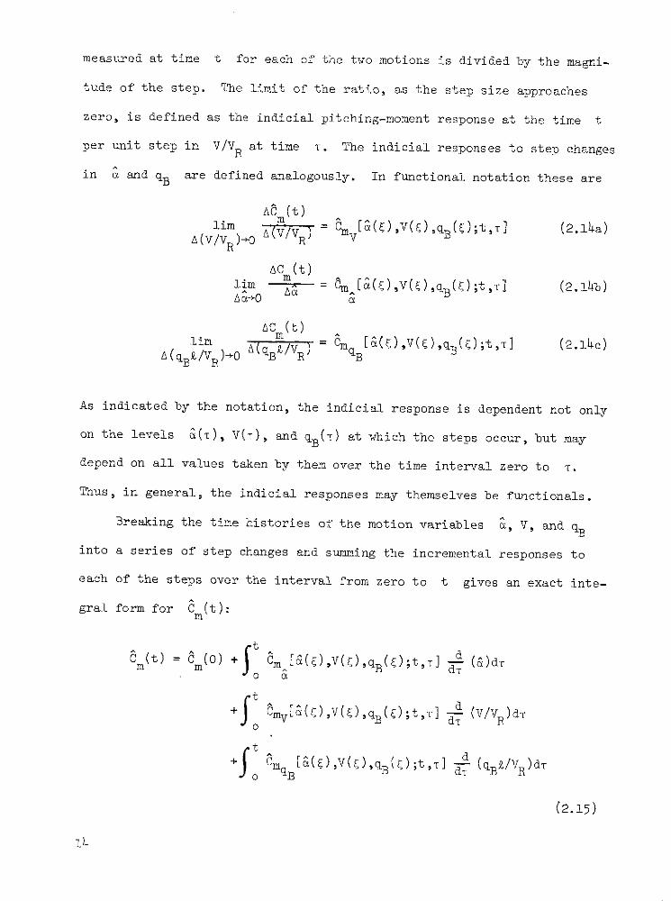
measured at time t for each of the two motions is divided by the magni-

tude of the step. The limit of the ratio, as the step size approaches

zero, is defined as the indicial pitching-moment response at the time t

per unit step in V/V R at time T. The indicial responses to step changes

in a and qB are defined analogously. In functional notation these are

R R V

AC (t)

ur - -(V"/V = CV[ ( ) V( ) ,q( ) t, (2.4a)

lm im ( = m [)(),V(),qB(C);t] (2.14b)Aa+0 a

ACm(t)m^

im A(q/VR = Cm [(),V(),qB(5);t,T] (2.14c)A(q B./VR )-*0 B R

As indicated by the notation, the indicial response is dependent not only

on the levels &(T), V(T), and qB(T) at which the steps occur, but may

depend on all values taken by them over the time interval zero to T.

Thus, in general, the indicial responses may themselves be functionals.

Breaking the time histories of the motion variables C, V, and qB

into a series of step changes and summing the incremental responses to

each of the steps over the interval from zero to t gives an exact inte-

gral form for Cm(t):

t

m(t) = C(O) + CmIt [-( S)'V()'q B();t'T] -d (&)dTm(0) B do a

+ mV(), ;t (v/v )dT0

+ C [&( ),V(E),qs(E);t, -] (qB/VR)dT

(2.15)

14

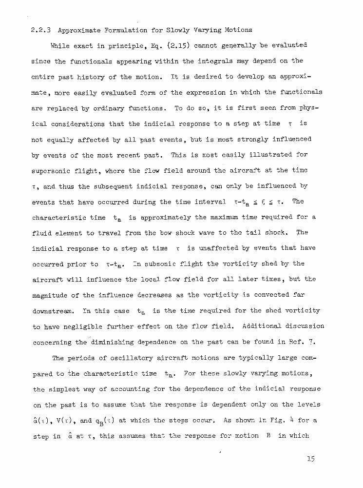
2.2.3 Approximate Formulation for Slowly Varying Motions

While exact in principle, Eq. (2.15) cannot generally be evaluated

since the functionals appearing within the integrals may depend on the

entire past history of the motion. It is desired to develop an approxi-

mate, more easily evaluated form of the expression in which the functionals

are replaced by ordinary functions. To do so, it is first seen from phys-

ical considerations that the indicial response to a step at time T is

not equally affected by all past events, but is most strongly influenced

by events of the most recent past. This is most easily illustrated for

supersonic flight, where the flow field around the aircraft at the time

T, and thus the subsequent indicial response, can only be influenced by

events that have occurred during the time interval T-t a 5 ' 5 T. The

characteristic time ta is approximately the maximum time required for a

fluid element to travel from the bow shock wave to the tail shock. The

indicial response to a step at time T is unaffected by events that have

occurred prior to T-ta. In subsonic flight the vorticity shed by the

aircraft will influence the local flow field for all later times, but the

magnitude of the influence decreases as the vorticity is convected far

downstream. In this case ta is the time required for the shed vorticity

to have negligible further effect on the flow field. Additional discussion

concerning the diminishing dependence on the past can be found in Ref. 7.

The periods of oscillatory aircraft motions are typically large com-

pared to the characteristic time ta. For these slowly varying motions,

the simplest way of accounting for the dependence of the indicial response

on the past is to assume that the response is dependent only on the levels

&(T), V(t), and qB(T) at which the steps occur. As shown in Fig. 4 for a

step in & at T, this assumes that the response for motion B in which

15

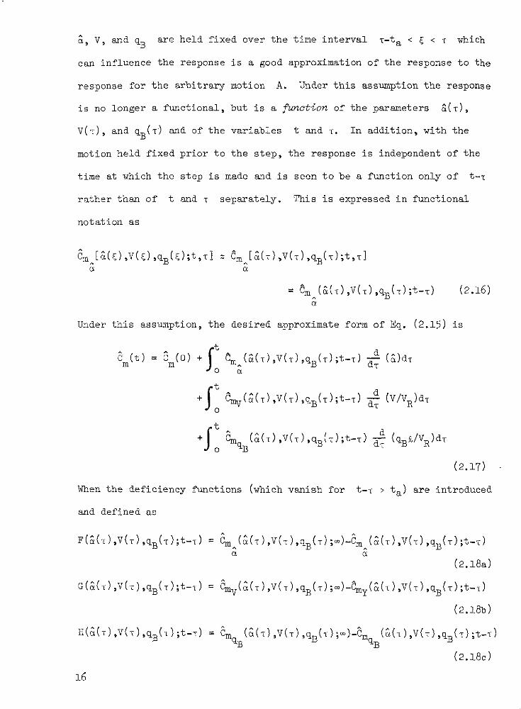
&, V, and qB are held fixed over the time interval T-ta < < T which

can influence the response is a good approximation of the response to the

response for the arbitrary motion A. Under this assumption the response

is no longer a functional, but is a function of the parameters &(T),

V(T), and qB(T) and of the variables t and T. In addition, with the

motion held fixed prior to the step, the response is independent of the

time at which the step is made and is seen to be a function only of t-T

rather than of t and T separately. This is expressed in functional

notation as

am a[a(),V(),qB();t,T] M &[&(T),V(T),qB(T);t,T]

= m^ (&a(),V(T),qB (T);t-T) (2.16)

Under this assumption, the desired approximate form of Eq. (2.15) is

Cm(t) = m(0) + em^(&(T),v(T),q(r);t-T) - (&)dTo a

+t -(),V(T), (T);-r) (v/v )dT

+ o mB(&(T),(r)(),qB(T);t-) -T (qBs/v)adT

(2.17)

When the deficiency functions (which vanish for t-T > ta) are introduced

and defined as

F(&(T),V(T)q B(T);t-T) = Cm (&(T),V(T),qB(T);o)-Cm^(&(T),V(.T),qB(T);t-T)

(2.18a)G(&(T) ,v(T),qB(T);t-T) = Cmv(&(T),v() , V(T),qB(T);t-T)

(2.18b)

H(a() V(-),qB(r);t-r) = amqB (&(),V(T),qB()) )CmqB (&(T),V(T),q B(U);tTr)

(2.18c)

16

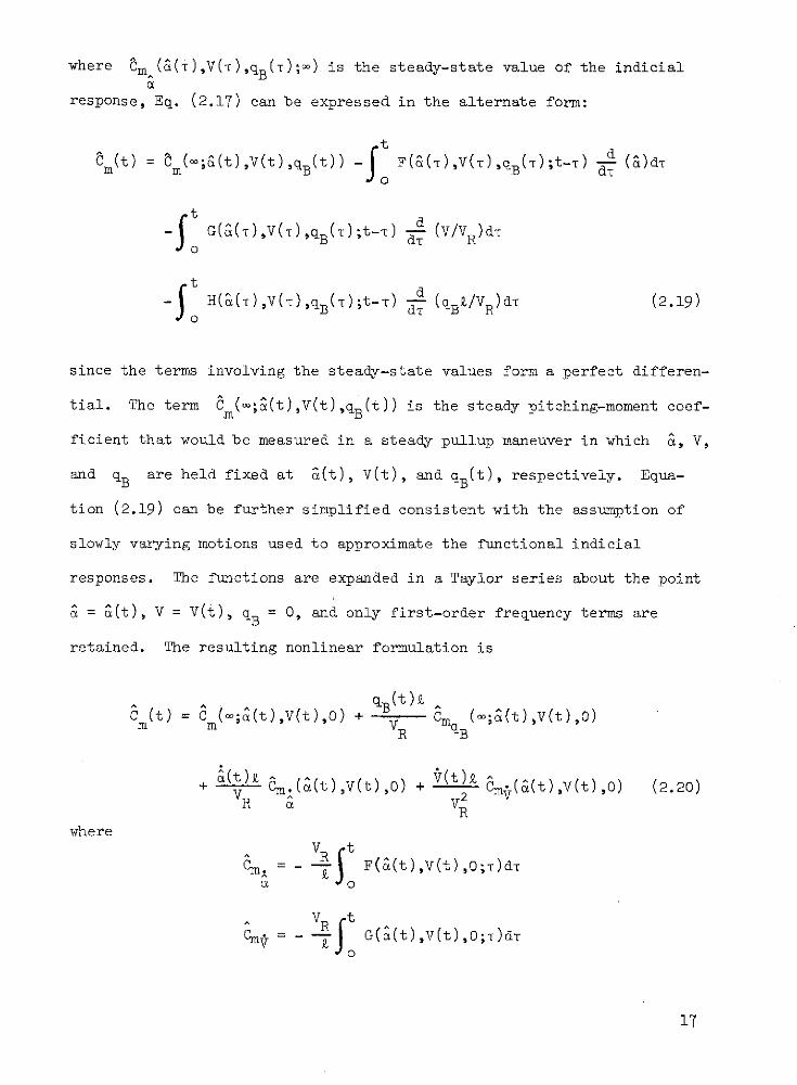
where Cm (&(T),V(W),qB();m) is the steady-state value of the indicial

response, Eq. (2.17) can be expressed in the alternate form:

r(t) = m;(t),V(t)q(t)) -( F(&(T),V(T),qB(T);t--C) -! (&)dT

ft a

- G(&(T),V(T),q(T);t-C) -- (V/VR)dt

tTd

- H(&(T),V(T),q(T) ;t-r) B (qBR/VR)d- (2.19)

since the terms involving the steady-state values form a perfect differen-

tial. The term m(m;^(t),V(t),qB(t)) is the steady pitching-moment coef-

ficient that would be measured in a steady pullup maneuver in which &, V,

and qB are held fixed at &(t), V(t), and qB(t), respectively. Equa-

tion (2.19) can be further simplified consistent with the assumption of

slowly varying motions used to approximate the functional indicial

responses. The functions are expanded in a Taylor series about the point

a = (t), V = V(t), qB = 0, and only first-order frequency terms are

retained. The resulting nonlinear formulation is

C (t) = C (;a(t),V(t),0) + R Cm B(m;&(t),V(t),0)m m V

+ () m.(&(t),V(t),) + V(t)_ aim.(&(t),V(t),o) (2.20)R a V2

where

Cm = - - F(&(t),V(t),0;)dT

a o

V t

C = - -J G(&(t),V(t),0;r)dr

17

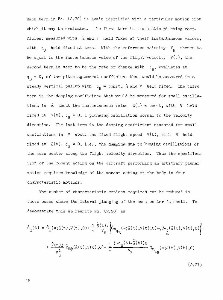
Each term in Eq. (2.20) is again identified with a particular motion from

which it may be evaluated. The first term is the static pitching coef-

ficient measured with a and V held fixed at their instantaneous values,

with qB held fixed at zero. With the reference velocity VR chosen to

be equal to the instantaneous value of the flight velocity V(t), the

second term is seen to be the rate of change with qB, evaluated at

qB = 0, of the pitching-moment coefficient that would be measured in a

steady vertical pullup with qB = const, & and V held fixed. The third

term is the damping coefficient that would be measured for small oscilla-

tions in a about the instantaneous value &(t) = const, with V held

fixed at V(t), qB = 0, a plunging oscillation normal to the velocity

direction. The last term is the damping coefficient measured for small

oscillations in V about the fixed flight speed V(t), with & held

fixed at &(t), qB = 0, i.e., the damping due to lunging oscillations of

the mass center along the flight velocity direction. Thus the specifica-

tion of the moment acting on the aircraft performing an arbitrary planar

motion requires knowledge of the moment acting on the body in four

characteristic motions.

The number of characteristic motions required can be reduced in

those cases where the lateral plunging of the mass center is small. To

demonstrate this we rewrite Eq. (2.20) as

am(t) = im(m;&(t),V(t),0)+ &(t m ( ;&(t),V(t),o)+yCm.(&(t),V(t),o)m m Y a

++ Vc (m;&(t),V(t),0)VR R B

(2.21)

18

The terms in Eq. (2.21) are identified by comparing them with those

obtained for the case of nonplunging motion at constant flight speed.

Under these conditions, = 0, qB = (1/y)a, and the last two terms of

Eq. (2.21) vanish. With the plunging of the mass center eliminated,

changes in & correspond to angular motion of the body about the fixed

YB axis. Thus the term (Cm + YCm.) is seen to be the planar pitchB a

damping coefficient that would be measured in a single-degree-of-freedom

experiment in which the body performs small angular oscillations about a

mean angle of attack, i.e., small oscillations in a about a = const,

with V held fixed and qB = (1/y)^. In a general motion, the contribu-

tions from the last two terms of Eq. (2.21) are not zero. However, for

motions in which the plunging is small, and where the flight speed makes

only small oscillations about a mean speed, the contributions from these

terms can be justifiably neglected since, in equations of vehicle motion,

they would appear only as products of (relatively small) damping terms.

In such cases the total moment acting on the aircraft is due to the con-

tributions from only two characteristic motions: steady angle of attack

and damping-in-pitch. Here V(t) need not appear explicitly within the

notation, it being understood that the characteristic motions will be

evaluated at a fixed speed equal to the mean value of the flight speed.

2.2.4 Extensions to Describe More General Motions

To obtain the approximate integral aerodynamic formulation, Eq.

(2.17), from the exact functional form, Eq. (2.15), the aircraft motions

were assumed to be slowly varying. The nonlinear indicial response for

these arbitrary large-amplitude motions was assumed to be the same as the

response to a motion with fixed past. For flutter motions involving

small-amplitude, high-frequency oscillations of the motion variables about

19

fixed mean values, the assumption of a constant past history is also

justified. Here the maximum excursions of the motion variables are small

and the motion can be considered to be generated by a series of steps

applied not at the instantaneous values but rather at the mean values of

the motion variables. The approximate integral form is thus valid for

flutter motions, but cannot be simplified as was done in the case of slowly

varying motions.

When considering large-amplitude motions of higher frequencies, the

simple assumption that the general nonlinear indicial response is the same

as the response for fixed past may no longer be adequate. A more precise

way to account for the dependence of the indicial response on past events,

for the planar motion discussed above, is to assume that the response to a

step at time T is dependent not only on the levels a(T), V(T), and

qB (), but also on their rates of change at the time of the step, ^(T),

V(T), and jB(T). This is illustrated in Fig. 4 for a step in &. In

motion C, a, V, and qB vary linearly in time with rates ^(T), V(T), and

B(T) over the time interval T-ta < < during which events may influ-

ence the subsequent response. The response to motion C is assumed to

be a closer representation of the response to the arbitrary motion A

than is the previously discussed response to motion B, whose past history

is held fixed. The approximate response is again a function rather than a

functional and is dependent on the parameters a(T), U(T), V(T), V(T),

qB(T), and B(T). Since the motion is uniquely specified by these param-

eters over the interval of influence prior to the step, the response is

again dependent on the time variable t-T rather than on t and T

separately. In functional notation this is indicated as

20

Cm ^ [&(),v(),qB( );t ,TI

=M (&(T),(T),V(T),(TI,qB(T)1B(TI;t-f) (2.22)

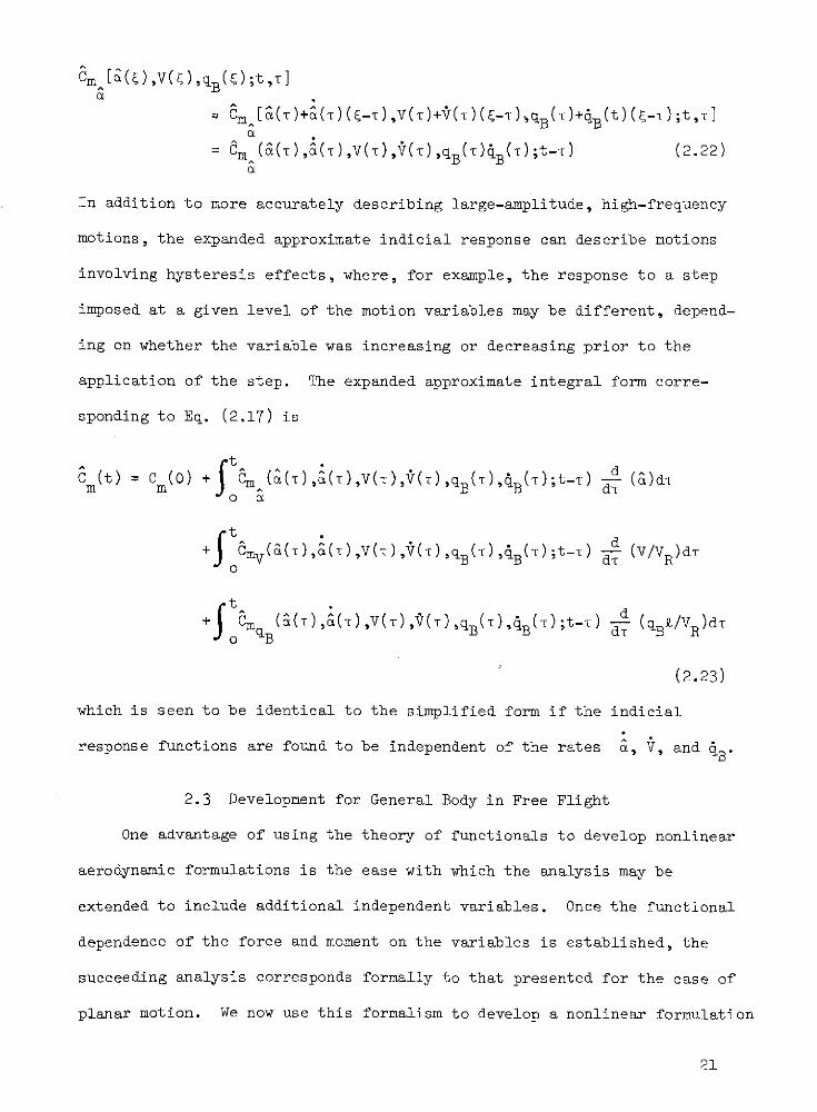
In addition to more accurately describing large-amplitude, high-frequency

motions, the expanded approximate indicial response can describe motions

involving hysteresis effects, where, for example, the response to a step

imposed at a given level of the motion variables may be different, depend-

ing on whether the variable was increasing or decreasing prior to the

application of the step. The expanded approximate integral form corre-

sponding to Eq. (2.17) is

m(t) Cm(0) + ((),(),V(),(T),qB (T),B();t- )

o CL

0

(2.23)

which is seen to be identical to the simplified form if the indicial

response functions are found to be independent of the rates ^, V, and AB.

2.3 Development for General Body in Free Flight

One advantage of using the theory of functionals to develop nonlinear

aerodynamic formulations is the ease with which the analysis may be

extended to include additional independent variables. Once the functional

dependence of the force and moment on the variables is established, the

succeeding analysis corresponds formally to that presented for the case of

planar motion. We now use this formalism to develop a nonlinear formulation

21

for a general body in free flight. Under the same restrictions on the

altitude and flight speed variations as were imposed on the planar case,

the force and moment acting on the body are dependent solely on the veloc-

ity and angular velocity history of the motion. The reactions and the

motion variables can be expressed in terms of their components resolved

in the body-fixed axes or, equivalently, by their components resolved in

the aerodynamic axis system. The resulting nonlinear formulations are

equivalent, but lead to different sets of characteristic motions from

which the total reactions are determined. However, as will be seen, the

importance of coning motion is evidenced by the fact that it appears as

one of the characteristic motions of the formulations developed in both

axis systems.

2.3.1 Body-Fixed Axes

The components of the flight velocity vector resolved in the body-

fixed axes, uB, vB, wB, are related to V, , V through Eqs. (2.1) and

(2.7). Thus the expanded dependence of the pitching-moment coefficient

can be specified as a functional of the form

m(t) = E[^(5), (,B,V( ),pB()B() ,rB()] (2.24)

The formulation of the nonlinear indicial responses and of the exact and

approximate integral forms for C (t) parallels that of the planar case,

Eqs. (2.14), (2.15), and (2.17), respectively. When the integral form is

expanded about the point & = &(t), = (t), V = V(t), pB = qB = rB = 0,

and only terms linear in the rates are retained, the resulting nonlinear

formulation corresponding to Eq. (2.20) is

22

S(t) Z t

q B(t) C ( B(t) ,V()) + V Ct) ((t) (t)(t)

+ V ^ +

R a VR B

+ v(t) Cm ( (t), ' (t),v(t)) (2.25)V2 V

where, for brevity, the zeros corresponding to pB' qB, rB have been

omitted.

Just as was done in the planar case, the formulation can be further

simplified for motions where the plunging of the mass center is small and

where the flight speed makes only small oscillations about a mean speed.

As before, we rewrite Eq. (2.25) and, guided by Eq. (2.11), neglect terms

multiplied by yqB-g + pByr +(- pB ), and V (their contributions vanish

identically in the case of zero plunging and constant flight speed). The

reference velocity VR is taken as the mean flight velocity V(t) and is

omitted from the functional notation of Eq. (2.25) for conciseness. The

simplified nonlinear formulation is

^ ^ 1 ^Cm(t) = Cm( ) + (Cmq (;^,M) + m (

+ _ (Vmr( ,) Ym(,)) +-- (.1 8B

Equation (2.26) is identical to Eq. (22) of Tobak and Schiff, 1 0 derived

for the case of constant flight speed. Analogous expressions for the

23

other moment coefficients C and C , and for the force coefficients CX

CY1 iZ are obtained by substituting them wherever im appears in

Eq. (2.26).

Each term of Eq. (2.26) is associated with a particular motion from

which it may be evaluated. The first two terms are identified by compar-

ing them with those previously obtained for the case of planar motion,

where pB = 0, B = const = 0. The first term is thus the pitching-moment

coefficient that would be measured in a steady planar motion with &,

(and V) held fixed. The term ( q +yCm.) is the planar damping-in-pitch

coefficient that would be measured for small angular oscillations in a

about fixed &, with B held fixed at 3(t) and pB = 0. Similarly,

(Cmr -YCm-) is the change in the pitching-moment coefficient due toB 8

damping-in-yaw motion (small angular oscillations in about fixed 6,

with a held fixed, pB = 0). As was pointed out in Ref. 10, the term

(Cmr -YCm) and the analogous term in C n(t), (n +YCn.), are the cross-B nB a

coupling terms normally excluded in the classical treatment. These terms

are missed by attempts to generalize to the nonlinear case from linear

formulations based on the principle of superposition.

The last term in Eq. (2.26) is identified by comparing it to the

result that would be obtained for the case of steady coning motion

(a = const, R = const, $ = const), where, as seen from Eq. (2.12), pB = ;

qB = ~ , rB = aC. When these conditions are substituted in Eq. (2.25),

the result is

= ) + v (Y (~,m) + (M;&) + r ( , ))m VqB B

(2.27)

24

The group (yC PB CmqgB+aCm rB is thus seen to be the rate of change with

;, evaluated at $ = 0, of the pitching-moment coefficient measured in

steady coning motion, and is designated C.(m;&,).

In summary, Eq. (2.26) suggests that for the free flight of a general

body with small plunging and near-constant flight speed, the total moment

may be compounded of the contributions from four characteristic motions:

steady angle of attack and sideslip, planar pitch and yaw oscillations at

constant angles of attack and sideslip, and coning at steady angle of

attack and sideslip. These motions are illustrated schematically in

Fig. 5.

2.3.2 Aerodynamic Axes

As can be seen in section 2.1, the velocity vector of a general

motion can be specified in the aerodynamic axes by the scalar variables

6, i, V. The angular velocity vector is specified by B', q, r or,

equivalently, by X, q, r, since pB is related to 3 and through

Eq. (2.4). The pitching-moment coefficient in the aerodynamic axes,

Cm(t), thus may be specified as a functional of the form

C m(t) = (2.28)

Proceeding formally, one finds that the nonlinear formulation in the aero-

dynamic axes corresponding to Eq. (2.25) is

C (t) C (w;6(t),p(t),V(t)) + t)Cm.(m;(t) (t),V(t))m m V

+ t Cm(_;6(t) ,(t),V(t)) + r(t)kVR V--V-- Cmr("; (t),(t),V(t))

+ 6(t)_ ' Cm.(6(t),(t),V(t)) + r Cm.(6(t),I(t),V(t))

VR 6 VR

+ (t Cmv((t),' ( t ) ,V(t)) (2.29)

VR

25

As before, Eq. (2.29) may be simplified in the case of small plunging and

near-constant flight speed by rearranging terms and neglecting those terms

multiplied by q-o, r-c , and V (which vanish identically for zero plunging

and constant flight speed, e.g., Eq. (2.10)) to obtain

Cm(t) = Cm(-;6,) + V (Cm (- ; 6 ,) + YCm.(6'4)) + -Cm.(6)

+ - (YCm.(c;6,) + 6Cmr(-;6,)) (2.30)

Analogous expressions hold for the other force and moment coefficients.

The characteristic motions from which the terms of Eq. (2.30) are evaluated

differ from those in the body-fixed axes.- Here the term (Cm +YCm ) is the

planar damping-in-pitch coefficient that would be measured in a nonplung-

ing motion for small oscillations of the resultant angle of attack a

about fixed a with 4 and V held fixed, X = 0. This term is designated

Cm.(6,). The term Cm. is the change in the pitching-moment coefficienta 4

due to damping-in-roll motion (small oscillations in 4 about fixed

with a = const, V = const, A = 0). When the conditions of steady coning

motion (q = 0, r = 6;, A = y;) are substituted in Eq. (2.29), it can be

shown that the term (6Cmr+yCm.) is the rate of change with coning rate

4, evaluated at = 0, of the pitching-moment coefficient that would

be measured in coning motion, and this term is designated Cm.(m ;,)

Thus

Cm.(6,)) = Cmq(-;6,0) + yCm.(6,)) (2.31a)a 6

Cm.(;6,4) = YCm.(;6,4) + 6 Cmr (-;6,) (2.31b)

In the aerodynamic axis system, the characteristic motions are: steady

resultant angle of attack and bank angle 4, pitch and roll oscillations

26

at steady angles of attack and bank, and coning at steady resultant angle

of attack with fixed bank angle. These motions are illustrated

schematically in Fig. 6.

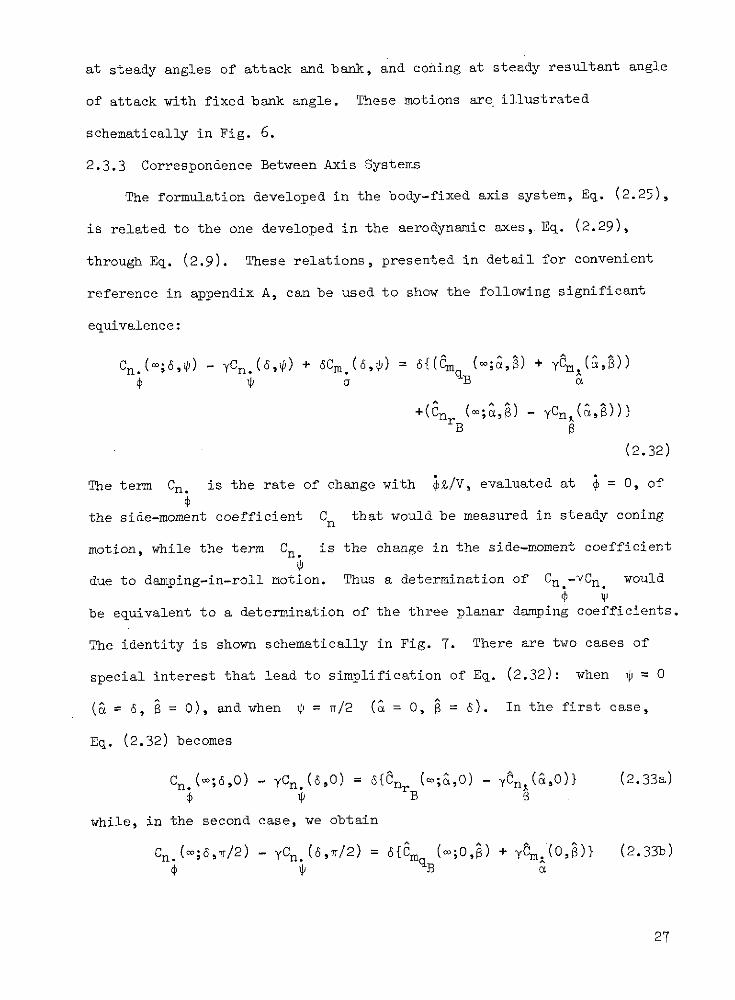
2.3.3 Correspondence Between Axis Systems

The formulation developed in the body-fixed axis system, Eq. (2.25),

is related to the one developed in the aerodynamic axes, Eq. (2.29),

through Eq. (2.9). These relations, presented in detail for convenient

reference in appendix A, can be used to show the following significant

equivalence:

Cn.(-;6,I) - YCn.(6,) + Cm.(6,,) = 6{(iim(q;& ,) + yrm , ))4, (

+(Cnr (o;a,8) - yCn~(8,))}B B

(2.32)

The term Cn. is the rate of change with RZ/V, evaluated at = 0, of

the side-moment coefficient Cn that would be measured in steady coning

motion, while the term Cn. is the change in the side-moment coefficient

due to damping-in-roll motion. Thus a determination of Cn.-YCn. would

be equivalent to a determination of the three planar damping coefficients.

The identity is shown schematically in Fig. 7. There are two cases of

special interest that lead to simplification of Eq. (2.32): when p = 0

(^ = 6, = 0), and when = Tr/2 (a = 0, = 6). In the first case,

Eq. (2.32) becomes

Cn.(m;6,0) - yCn.(6,0) = 6{Inr (%;&,0) - yCn,(&,0)} (2.33a)

while, in the second case, we obtain

Cn.(-;6,7/2) - yCn.(6,w/2) = 6{Cm (m ;0,) + ym~*(0, )} (2.33b)

27

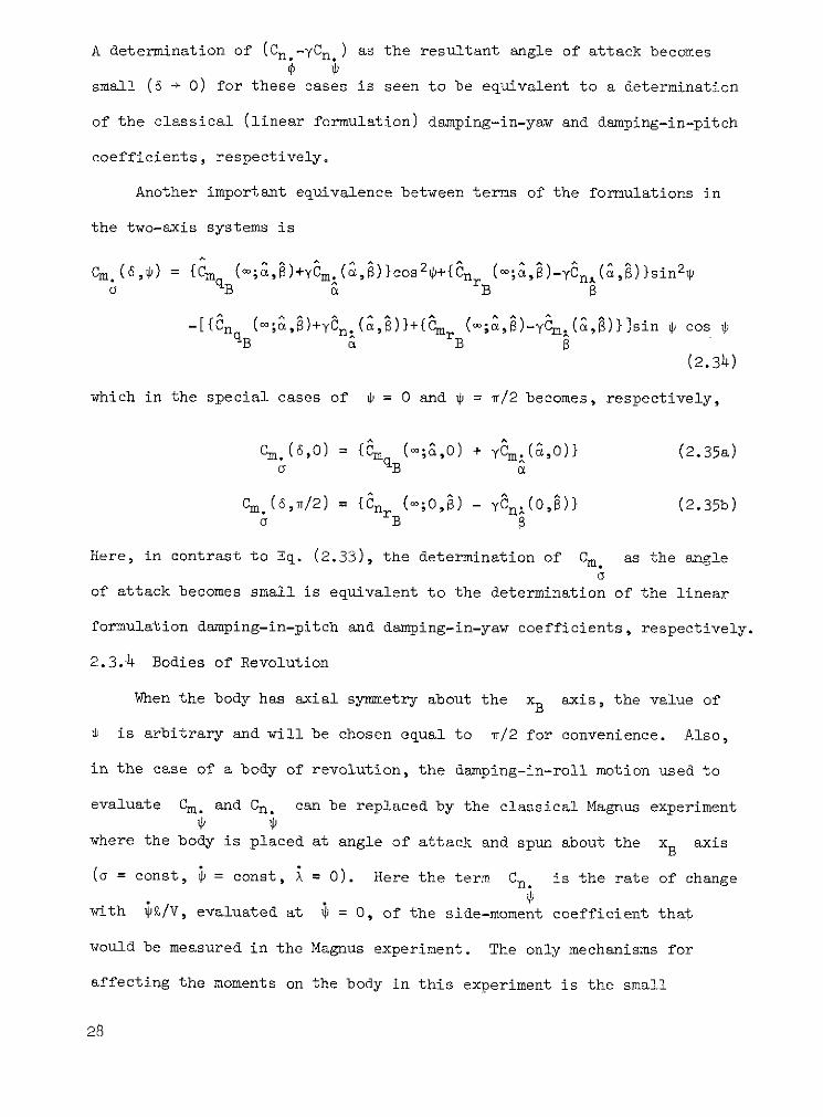
A determination of (Cn.-yCn.) as the resultant angle of attack becomes

small (6 - 0) for these cases is seen to be equivalent to a determination

of the classical (linear formulation) damping-in-yaw and damping-in-pitch

coefficients, respectively.

Another important equivalence between terms of the formulations in

the two-axis systems is

Cm.(6,) = {Cm q m.( os2 (;a,)-yC,(&,)}sin2o a B

-[CnqB (^ , ^)+Y ( cl,)}+{r ( ;a,8)-i.(&,)}]sin , cos 4

(2.34)

which in the special cases of = 0 and 4 = w/2 becomes, respectively,

Cm.(6,0) = {Cmq (-;&,0) + yCm.(&,0)} (2.35a)

Cm.(6,w/2) = {anr (m;0,8) - YCn.(0,I)} (2.35b)oB

Here, in contrast to Eq. (2.33), the determination of Cm. as the angle

of attack becomes small is equivalent to the determination of the linear

formulation damping-in-pitch and damping-in-yaw coefficients, respectively.

2.3.4 Bodies of Revolution

When the body has axial symmetry about the xB axis, the value of

0 is arbitrary and will be chosen equal to 7/2 for convenience. Also,

in the case of a body of revolution, the damping-in-roll motion used to

evaluate Cm. and Cn. can be replaced by the classical Magnus experiment

where the body is placed at angle of attack and spun about the xB axis

(a = const, i = const, = 0). Here the term Cn. is the rate of change

with iZ/V, evaluated at = O, of the side-moment coefficient that

would be measured in the Magnus experiment. The only mechanisms for

affecting the moments on the body in this experiment is the small

28

asymmetry of the flow field produced by viscous shear at the body surface.

Thus numerous experimental investigations (e.g., Regan and Horanoff,14

Platou and Sternberg,15 Platou 16) and a viscous theory (Sedney 17 ) have

shown that, when measured in this manner, the term Cn. and the corre-

sponding side force term, Cy., for a body of revolution are extremely

small. Additionally, Schiff and Tobak 5 have demonstrated experimentally

that, at least for a 100 half-angle cone, the term Cn. can be neglected

in comparison with Cn., the change in the side moment due to steady con-

ing motion. In this case the determination of Cn. alone, for small

resultant angle of attack, is seen from Eq. (2.33b) to be equivalent to

the determination of the linear damping-in-pitch coefficient.

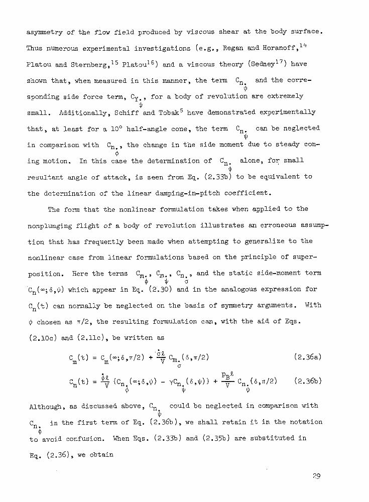
The form that the nonlinear formulation takes when applied to the

nonplunging flight of a body of revolution illustrates an erroneous assump-

tion that has frequently been made when attempting to generalize to the

nonlinear case from linear formulations based on the principle of super-

position. Here the terms Cm., Cm., Cn., and the static side-moment term

Cn(; 6, ) which appear in Eq. (2.30) and in the analogous expression for

Cn(t) can normally be neglected on the basis of symmetry arguments. With

' chosen as w/2, the resulting formulation can, with the aid of Eqs.

(2.10c) and (2.11c), be written as

C (t) = Cm(;6,w/2) + - Cm.(,wrr/2) (2.36a)

Cn(t) = {Cn.(m;6,) - yCn.(6,)} + - Cn.(6,/2) (2.36b)

Although, as discussed above, Cn. could be neglected in comparison with

Cn. in the first term of Eq. (2.36b), we shall retain it in the notation

to avoid confusion. When Eqs. (2.33b) and (2.35b) are substituted in

Eq. (2.36), we obtain

29

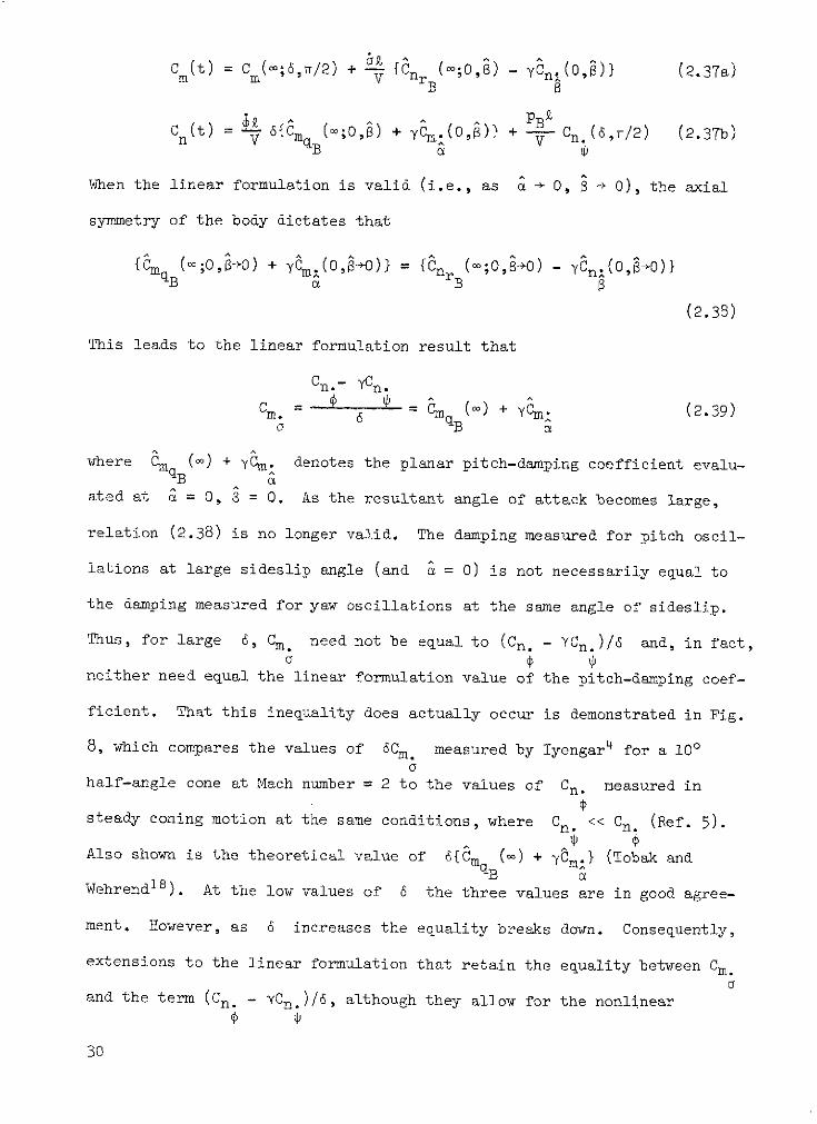
Cm(t) = Cm 6,/2) + i{Cnr (m;o0,) - YCn(0o,)} (2.37a)C (t) = C ;6m/2) V f PBB B

Cn (t) 6{Cmq (m;0,) + c.(0',B)} + - Cn.(6,w/2) (2.3Tb)a

When the linear formulation is valid (i.e., as & - 0, B - 0), the axial

symmetry of the body dictates that

{CmqB(c;0,-+0) + ym.(0,-+0O)} = {Cn (;0,O80) - yCn.(0, 0)}a B

(2.38)

This leads to the linear formulation result that

Cn.- YCn.

Cm-. 6 ) + yC. (2.39)U B a

where Cm ((m) + yCm. denotes the planar pitch-damping coefficient evalu-

ated at a = 0, = 0. As the resultant angle of attack becomes large,

relation (2.38) is no longer valid. The damping measured for pitch oscil-

lations at large sideslip angle (and & = 0) is not necessarily equal to

the damping measured for yaw oscillations at the same angle of sideslip.

Thus, for large 6, Cm. need not be equal to (Cn. - YCn.)/6 and, in fact,

neither need equal the linear formulation value of the pitch-damping coef-

ficient. That this inequality does actually occur is demonstrated in Fig.

8, which compares the values of 6Cm. measured by Iyengar4 for a 100a

half-angle cone at Mach number = 2 to the values of Cn. measured in

steady coning motion at the same conditions, where Cn. << Cn. (Ref. 5).

Also shown is the theoretical value of 6{C m(-) + aim.} (Tobak and

Wehrendl8). At the low values of 6 the three values are in good agree-

ment. However, as 6 increases the equality breaks down. Consequently,

extensions to the linear formulation that retain the equality between Cm.

and the term (Cn. - YCn.)/6, although they allow for the nonlinear

30

behavior of Cm. with increasing angle of attack, will lead to false

results, In particular, when (Cn. - yCn.)/6 is incorrectly forced to

equal Cm., the difference between the assigned value and the actual one

must be absorbed in the remaining term of the side-moment equation,

{pBZ/V)Cn.. As discussed by Levy and Tobak,9 this may cause methods that

extract nonlinear aerodynamic coefficients from free-flight data, if based

on such an aerodynamic formulation, to assign an unrealistically large

value to Cn., although the value determined in the classical Magnus

experiment would bp negligibly small.

2.3.5 Potential Application to Airplane Spins

The ability to predict the pre-stall and post-stall spin behavior of

high performance aircraft is currently hampered by the inadequacies of the

linear aerodynamic moment system. The striking similarity between coning

motion and the steady spin of an aircraft suggests that a moment formula-

tion similar to Eq. (2.25) (or, alternately, Eq. (2.29)) will properly

describe the aerodynamic reactions on a spinning airplane. It is known,

however, that in the establishment of a spin the large asymmetric regions

of separated flow on the wings of the vehicle cause the aerodynamic reac-

tions to be highly nonlinear functions of the spin rate, even at low spin

rates. This contradicts the assumption, used in the development of Eq.

(2.25), that the reactions are linear functions of the rates. It is

anticipated that by expanding the integral form for C m(t) corresponding

to Eq. (2.17) about the point pB = PB(t) (the instantaneous spin rate)

rather than about pB = 0, a formulation corresponding to Eq. (2.25) could

be obtained which would describe the nonlinear behavior of the aerodynamic

reactions with coning rate as well as with angle of attack and sideslip.

In such a formulation pB(t) would, of necessity, be retained in the

notation.

31

3. NUMERICAL FLOW-FIELD SOLUTION

The previous chapter has shown that the nonlinear aerodynamic force

and moment acting on a body performing large-amplitude nonplanar motions

can be compounded of the contributions from four characteristic motions:

steady angle of attack, pitch oscillations, either roll or yaw oscilla-

tions, and coning motion. It would be desirable to be able to apply

methods of computational fluid dynamics to compute the flow fields about

bodies performing these characteristic motions and so obtain their con-

tributions to the aerodynamic reactions. Extensive study of the steady

angle-of-attack case has led to the development of many numerical finite-

difference methods for computing the steady inviscid flow field about two-

and three-dimensional bodies for subsonic through hypersonic Mach numbers.

The computation of the nonsteady flow fields generated by the oscillatory

motions is more difficult. Here the flow variables are functions of time

as well as of position, and thus the solution requires increased computa-

tion and larger computer data storage capacity than is necessary for the

steady flow case. Coning motion, shown to have special significance in

the nonlinear moment formulation, generates a flow field more amenable to

numerical solution than do those of the oscillatory cases, since to an

observer fixed on the coning body the surrounding flow is steady. Hence,

techniques developed for the solution of steady flow fields can be applied

to coning motion.

The study of steady supersonic flow has led to the development of a

class of accurate numerical finite-difference methods termed marching

methods. By taking advantage of the fact that the equations governing a

supersonic flow are hyperbolic in the streamwise direction, the use of

such methods advances an initial solution, specified at one transverse

32

plane, in the streamwise direction to obtain the entire flow field. These

methods enable the solution of the full nonlinear gasdynamic equations,

rather than the simplified equations obtained by the introduction of a

velocity potential. The solutions obtained are therefore valid for flows

at hypersonic Mach numbers where vorticity is generated by strong curved

shock waves, as well as for flow at lower supersonic Mach numbers. One

such method, the noncentered second-order scheme introduced by MacCormack 11

and developed by Kutler and Lomax 12 as a shock-capturing technique, has

been shown to be both accurate and versatile. Results of computations of

the complex steady hypersonic flow field surrounding a proposed space

shuttle orbiter, obtained using this technique, show excellent agreement

with experiment and with results obtained from a three-dimensional method

of characteristics (Rakich and Kutlerl9). In a shock-capturing technique,

the equations are expressed in conservation-law form and the finite-

difference scheme is applied uniformly at all points of a computational

mesh which extends into the undisturbed free stream ahead of the bow shock

wave. The jump in the flow variables across the shock is spread over

several points of the mesh. In a sharp-shock technique, the bow shock is

treated as a discontinuity and the Rankine-Hugoniot relations are used to

determine the flow conditions immediately behind the shock. One advantage

of the shock-capturing technique is its ability to determine the position

and strength of the bow shock without special computer coding. A second

and more important advantage is its ability to determine the position and

strength of embedded shock waves, such as the crossflow shocks that are

seen on the leeward side of a body at large angles of attack, if they

occur within the flow field. Because of its accuracy and simplicity, the

shock-capturing technique was extended to the case of a body in coning

motion in a supersonic stream.

33

3.1 Method of Solution

The nonlinear Eulerian gasdynamic equations are solved numerically

to determine the totally supersonic inviscid flow field about a pointed

body in coning motion. A body-fixed cylindrical coordinate system, desig-

nated the computational system, is introduced. The origin of these coordi-

nates lies at the center of gravity of the body, with s, the axial coordi-

nate, aligned with the negative xB axis. The radial coordinate T lies

in planes normal to the xB axis (i.e., in crossflow planes) as illustrated

in Fig. l(a). The circumferential angle, 6, is seen to be measured from

the resultant angle-of-attack plane. In coning motion at fixed coning rate

;, the flow is time-invariant with respect to an observer fixed in the com-

putational coordinate system. Since the flow field is everywhere super-

sonic, the gasdynamic equations are hyperbolic in the axial direction. A

computational mesh is established between the body surface and the free

stream ahead of the bow shock wave in planes normal to the s axis. With

the flow field specified at an initial data plane, s = sinitial' MacCormack's

method is used to march the solution in the s direction over the length

of the body. At the outer edge of the mesh, the flow variables are assigned

free-stream values, while at the inner edge, the flow is kept tangent to

the body. With the complete flow field thus determined, the forces and

moments are obtained from a subsequent integration of the surface pressure

distribution.

Computations have been carried out for conical bodies of circular and

elliptical cross section. An approximate initial solution was generated

at the initial data plane by assuming the flow upstream to be that about a

cone at angle of attack and yaw, with a uniform sidewash velocity. Note

that although the body geometry is conical, the free-stream sidewash

generated by coning motion is a function of axial position along the body,

34

and the resulting flow field is not conical. Details of the method and a

discussion of the approximate starting solution are given below.

The computations were carried out on an IBM 360/67 computer linked to

a cathode-ray tube graphics device. The graphics unit, which possesses

man-machine interaction capability, was used to study the flow field as it

developed, and to control any numerical instabilities that evolved.

Approximately 50 minutes of computer time were required per case (one

angle of attack at one coning rate).

3.2 Gasdynamic Equations

The equations governing the unsteady inviscid flow of a non-heat-

conducting perfect gas around a body performing an arbitrary motion, writ-

ten with respect to a body-fixed coordinate system whose origin is at the

center of gravity of the body, can be expressed as

(mass) ~ (p) + div( p) = 0 (3.la)

(momentum)

- (pV) + grad p + pV * grad V + V div(pV) + p x + (tcg

+ (5)x + rx(exr)]= 0 (3.1b)

(energy)

-a (E) + div[(p+&)V] + 2 x- + ( ) + (5)x. + x(nx) pV = 0at dt()xV + 2x(xrj * pV 0g d

(3.1c)

(state) p = (Y-l)pe (3.1d)

where

r position vector in the body coordinate system

V(r,t) velocity vector (having components u, v, w) of the fluid at the

point r, measured relative to the body-fixed coordinates

35

V cg, velocity and angular velocity, respectively, of the

body-fixed coordinates measured with respect to

an inertial system

F = p[e+(1/2)1 12 ] total energy per unit volume of fluid

The terms 2px~x and px(_xr) in Eqs. (3.1b) and (3.1c) are Coriolis and

centrifugal force terms that appear because the body-fixed coordinate sys-

tem is noninertial.

In the case of steady coning motion, V = const, 0 = const, and thecg

flow field is time-invariant in the body-fixed coordinates. Under these

conditions, Eqs. (3.1) become

(mass) div(pV) = 0 (3.2a)

(momentum)

grad p + pV * grad r + V div(pV) + p[2 xV + x(nx3)] = 0 (3.2b)

(energy)

div[(p+.g)V] + [2x7 + 5x(x_)] * pV = 0 (3.2c)

Equation (3.2c) can be simplified upon recognizing that (Vx) * V =

* (VxV) = 0. Also it can be shown that with 5 = const,

curl[nx( xr)] = 0, and thus nx(nxF) can be expressed as the gradient of

a potential, i.e., nx( xy) = grad(-€/2). Substituting in Eq. (3.2c), and

using Eqs. (3.2a) and (3.1d), we obtain

pV • grad (e - D + 12) 0 (3.3)

This states that e - + I I2) is constant along streamlines of the

flow field. Since the motion under consideration is that of a body through

a uniform atmosphere at rest with respect to the inertial system, the con-

stant is the same for all streamlines, and Eq. (3.3) becomes

36

ye - ( + -1 V2 const = ye h (3.4a)

or

p Y-1 p[2h + D - (u 2 +v 2+w 2 )] (3.4b)2y o

The number of dependent variables is thus reduced from five (E, p, V) to

four (p, v), with p related to p and V through Eq. (3.4b).

When the coordinate system is specialized to the body-fixed computa-

tional system, the gasdynamic equations (3.2a) and (3.2b) can be written

in conservation-law form as

E' + F' + G' + H' = 0 (3.5)s T 0

where the subscripts denote differentiation and

pu pv pw

E' = p+pu 2 F' = puv 2' puwpuv Ip+pv2 pvw

puw pvw p+pw 2

pv2 2

1 puv + pT[2(w 2 w-w 3v)+A 1 2 T-s(W 2 +W 3 )]

' T p(v 2 _W2 ) + OT[2(W3u-wIw)+Iw2s-T(wI+W3)

2pvw + pT[2(lv-w2 u)+w 3 ( 2 T+w1 s)]

The components of the angular velocity vector of magnitude $, resolved

in the s,T,6 directions are, respectively, w, = -$ cos a,

W2 = $ sin a cos e, and w 3 = -a sin a sin 0. The energy equation is given

by Eq. (3.4b), while the centrifugal force potential, obtained from the

integration of grad(-$/2) = ~x(£~x), can be expressed as

S= 2 [(s sin G + T5cos a cos e)2 + (T sin 0)2]

For supersonic flow, Eq. (3.5) is hyperbolic with respect to s, and

thus can be integrated in the s direction. Specifically, u, the compo-

nent of the local flow velocity in the s direction, must be greater than

37

the local speed of sound at all points of the flow field. In regions

where this condition does not hold, such as in the subsonic nose region of

a blunted body, the marching method fails. In such a case the nonsteady

form of the gasdynamic equations would have to be integrated with respect

to time, and the steady solution would be obtained as the steady limit of

an unsteady flow.

It is generally advantageous, when flow problems are solved with the

use of finite-difference methods, to have the physical boundaries of the

flow field lie along coordinate surfaces of the computational coordinate

system. Under these conditions the application of the surface boundary

conditions is greatly simplified. Further, to improve the accuracy of the

solution, it is desirable to use a dense spacing of computational grid

points in those regions of the flow field where large gradients of the flow

variables are known or suspected to exist. Thus, in the present case, that

of flow over cones of circular and elliptical cross section, the annular

region of interest about the body (in the T,6 plane) is transformed into

a rectangular region (Fig. 9). A radial independent coordinate P is

chosen to map the region between the body surface and an outer boundary

into the region 0 :p : 1. The outer boundary is chosen to lie in the

undisturbed stream outside the bow shock wave. It is known that when a

cone of elliptical cross section is placed at incidence in a wing-like

attitude (i.e., with the semimajor axis of the ellipse normal to the flow

direction) rapid variations of the flow variables occur in the vicinity

of the semimajor axis. A circumferential independent variable n, depen-

dent on the body cross section, is therefore chosen to cluster the physi-

cal circumferential planes more closely in these regions. The

transformations are:

38

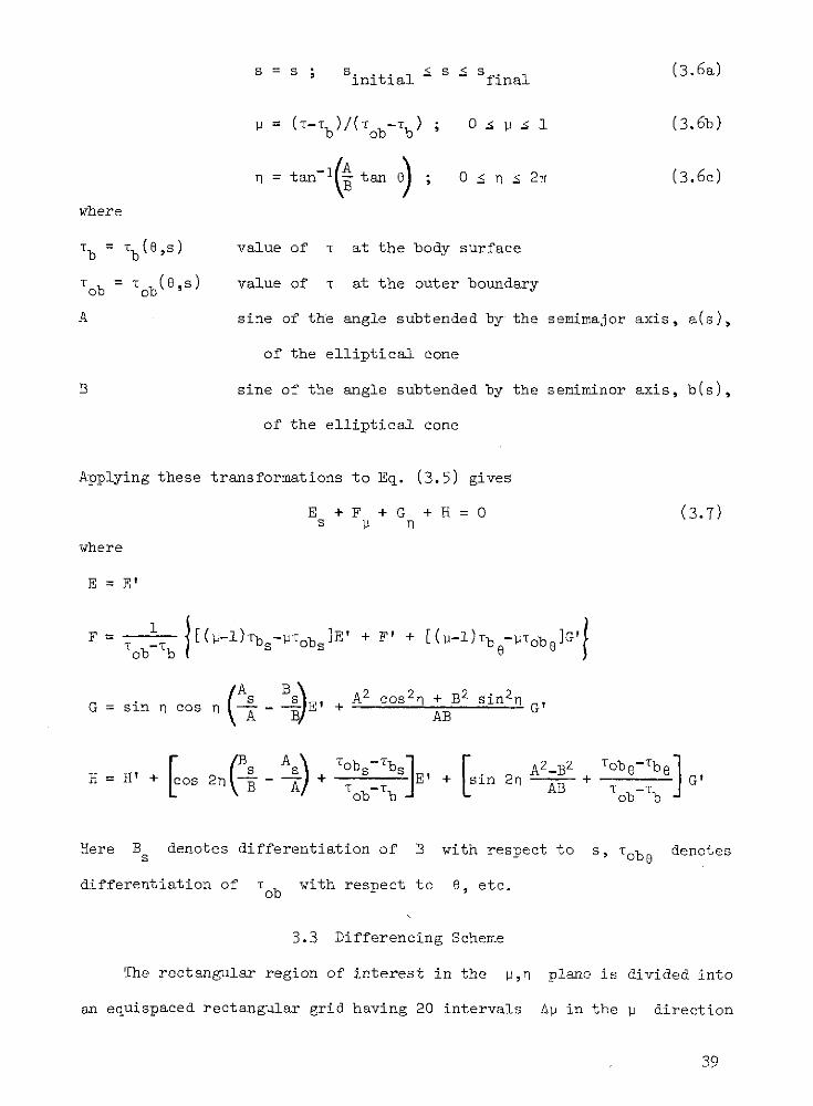
P= (T- Tb ob-b) ; 0 : i i 1 (3.6b)

I =tan-1 ( tan e) ; O 2r (3. 6c)

where

Tb b(,s) value of T at the body surface

Tob Tob(e,s) value of T at the outer boundary

A sine of the angle subtended by the semimajor axis, a(s),

of the elliptical cone

B sine of the angle subtended by the semiminor axis, b(s),

of the elliptical cone

Applying these transformations to Eq. (3.5) gives

E + F + G + H = 0 (3.7)s 11 T

where

E = E'

F = ob1 b [(p-l)Tbs-pTobs]E' + F' + [(V-l)Tb6-ITob]G'I

(As Bs A2 cos2 n + B 2 sin 2nG = sin n cos n E' + AB

H' +s As\ Tobb1 + A 2-B2 Tobe8b6

H = H' + os 2) + E' + in 2n -- + 'B A T-T b AB T ob-b

Here Bs denotes differentiation of B with respect to s, Tobe denotes

differentiation of Tob with respect to 0, etc.

3.3 Differencing Scheme

The rectangular region of interest in the p,n plane is divided into

an equispaced rectangular grid having 20 intervals Ap in the V direction

39

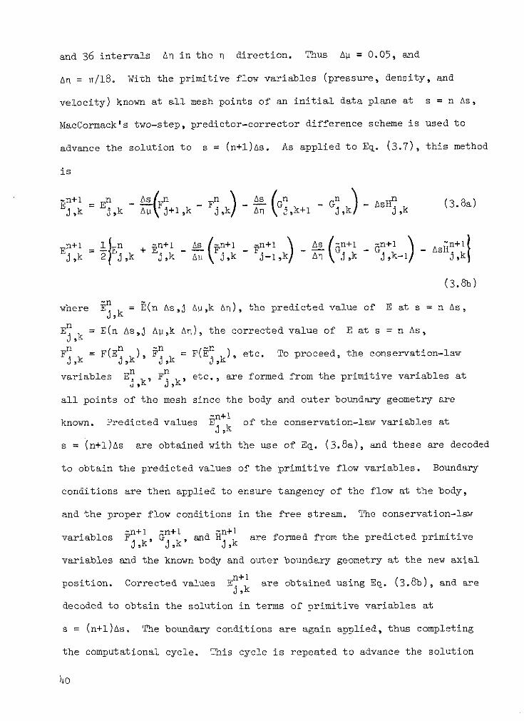
and 36 intervals An in the n direction. Thus AP = 0.05, and

An = w/18 . With the primitive flow variables (pressure, density, and

velocity) known at all mesh points of an initial data plane at s = n As,

MacCormack's two-step, predictor-corrector difference scheme is used to

advance the solution to s = (n+l)As. As applied to Eq. (3.7), this method

is

n1 = E - F _ asn n As O - n - AsHn (3.8a)j,k jk Ali j+1,k jk ,k+1 j,k/ j,k

En+ I En n+l As n+1 n+ k) As n+1 -n+1 An+1E_+ En --- - AsH

j,k 2 Jk j,k Ap j,k j-1, An jk j,k-i jk

(3.8b)

where i = (n As,j AV,k An), the predicted value of E at s = n As,j,k

En = E(n As,j AV,k An), the corrected value of E at s = n As,j ,k

Fn = F(En, ) , n, = (n ), etc. To proceed, the conservation-lawlk k jk

variables E n Fkn etc., are formed from the primitive variables atj,k' j,k'

all points of the mesh since the body and outer boundary geometry are

known. Predicted values En of the conservation-law variables atj ,k

s = (n+l)As are obtained with the use of Eq. (3.8a), and these are decoded

to obtain the predicted values of the primitive flow variables. Boundary

conditions are then applied to ensure tangency of the flow at the body,

and the proper flow conditions in the free stream. The conservation-law

-n+1 n+1 n+1variables F, G, and H are formed from the predicted primitive

j,k j,k j,,k

variables and the known body and outer boundary geometry at the new axial

position. Corrected values En + 1 are obtained using Eq. (3.8b), and arej,k

decoded to obtain the solution in terms of primitive variables at

s = (n+l)As. The boundary conditions are again applied, thus completing

the computational cycle. This cycle is repeated to advance the solution

40

from s = (n+l)As to s = (n+2)As, and so on over the entire length of

the body.

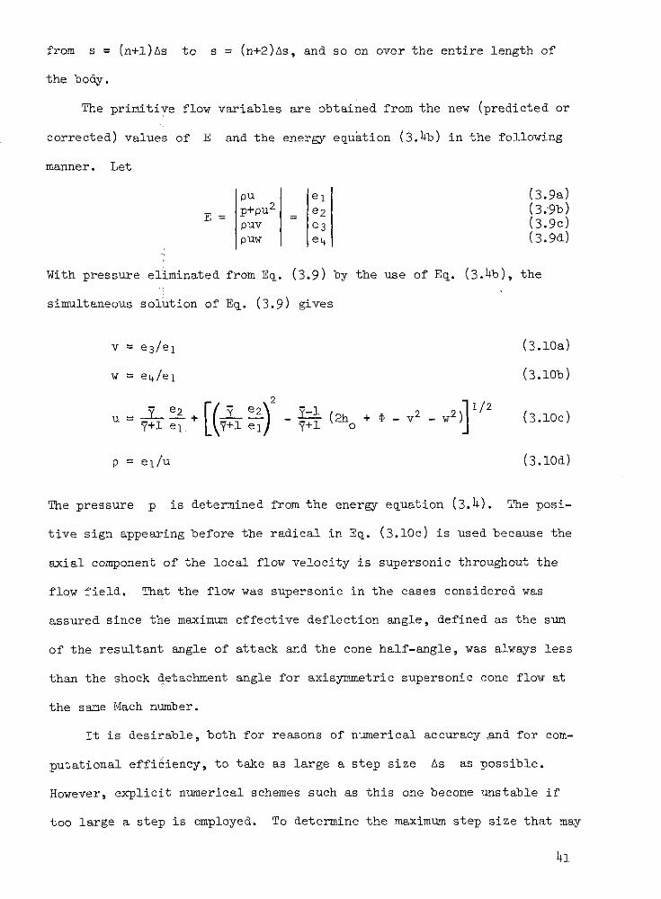
The primitive flow variables are obtained from the new (predicted or

corrected) values of E and the energy equation (3.4b) in the following

manner. Let

pu el (3.9a)

p+pu2 e 2 (3.'9b)E=puv e3 (3.9c)

puw eq (3.9d)

With pressure eliminated from Eq. (3.9) by the use of Eq. (3.4b), the

simultaneous solution of Eq. (3.9) gives

v = e3/e1 (3.10a)

w = eq/el (3.10b)

e 1 2 2 w 12

u = e - (2h + @ - v2 - ) (3.10c)7+1 el 1 el 7+1 0

p = el/u (3.10d)

The pressure p is determined from the energy equation (3.h). The posi-

tive sign appearing before the radical in Eq. (3.10c) is used because the

axial component of the local flow velocity is supersonic throughout the

flow field. That the flow was supersonic in the cases considered was

assured since the maximum effective deflection angle, defined as the sum

of the resultant angle of attack and the cone half-angle, was always less

than the shock detachment angle for axisymmetric supersonic cone flow at

the same Mach number.

It is desirable, both for reasons of numerical accuracy ,and for com-

putational efficiency, to take as large a step size As as possible.

However, explicit numerical schemes such as this one become unstable if

too large a step is employed. To determine the maximum step size that may

41

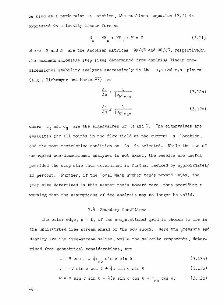
be used at a particular s station, the nonlinear equation (3.7) is

expressed in a locally linear form as

E + ME + NE + H = 0 (3.11)s P n

where M and N are the Jacobian matrices OF/DE and 3G/DE, respectively.

The maximum allowable step sizes determined from applying linear one-

dimensional stability analyses successively in the p,s and n,s planes

(e.g., Richtmyer and Morton2 0) are

As 1 (3.12a)

1 cOM max

As 1As (3.12b)An m

where aM and oN are the eigenvalues of M and N. The eigenvalues are

evaluated for all points in the flow field at the current s location,

and the most restrictive condition on As is selected. While the use of

uncoupled one-dimensional analyses is not exact, the results are useful

provided the step size thus determined is further reduced by approximately

10 percent. Further, if the local Mach number tends toward unity, the

step size determined in this manner tends toward zero, thus providing a

warning that the assumptions of the analysis may no longer be valid.

3.4 Boundary Conditions

The outer edge, p = 1, of the computational grid is chosen to lie in

the undisturbed free stream ahead of the bow shock. Here the pressure and

density are the free-stream values, while the velocity components, deter-

mined from geometrical considerations, are

u = V cos ao - ;Tob sin a sin 6 (3.13a)

v = -V sin a cos 6 + $s sin a sin 6 (3.13b)

w = V sin a sin 6 + $(s sin a cos e + Tob cos a) (3.13c)

42

At the sides (n = 0 and n = 27) of the computational grid, a periodic con-

tinuation principle is applied, i.e., p(u,n = 0) = p(l,n = 27),

P(P,n = 0) = p(P,n = 2 ), etc. The tangency boundary condition at the

body, = 0, is due to a scheme of Abbett 2 1 and is briefly summarized here.

The flow variables are known at the new axial position after the predictor

step. In general, the local flow velocity at the body is not tangent to

the body. A local two-dimensional Prandtl-Mayer expansion or an isentropic

compression is used as needed to turn the flow into the local tangent plane.

This satisfies the tangency condition and determines a corrected value of

the surface pressure. A corrected value of the surface density is then

determined since it is assumed that flow along surface streamlines is

isentropic. The magnitude of the corrected flow velocity is then deter-

mined from the energy equation, Eq. (3.4), while its direction is that

obtained from satisfying the tangency condition. This tangency condition

scheme has been shown to give good results. The surface flow conditions

for a circular cone at angle of attack computed by Kutler et al.22 using

this scheme were found to be in good agreement with the numerical results

of Babenko et al.2 3 and with the method of characteristics results of

Rakich.2 4

Crossflow shocks were observed to exist in the flow field for the high

angle-of-attack computations and to extend to the body surface. In such

cases, the assumption that the flow is isentropic along surface streamlines

is no longer valid. In principle, the value of surface entropy (used in

the tangency scheme to compute the corrected surface density) for points

behind the embedded shocks should be different from those points unaffected

by the shocks. However, if the embedded shocks are relatively weak this

refinement to the tangency condition can be justifiably neglected. This

43

was found to be the case in the present computations, and a single value

of surface entropy was used for all points on the surface.

3.5 Initial Solution

The flow field surrounding even a conical body is not conical when

the body is in coning motion since the sidewash velocity of the undisturbed

stream, measured by an observer on the body, is a function of axial position.

This is illustrated in Fig. 10(a) for the conical tip of a body in coning

motion. The velocity component normal to the angle-of-attack plane varies

linearly from stip sin at s = tip to initial in at s = initial'

changes direction at s = 0, and increases linearly with s behind the

mass center. The exact computation of the flow field upstream of the ini-

tial data plane at s = initil would require the use of a three-

dimensional, time-dependent technique with the steady solution approached

as the limit of an unsteady flow. To avoid this complication, an approxi-

mate initial solution, valid for bodies with conical tips and capable of

being generated by the marching method, is employed. The flow field

upstream of the initial data plane for the conical tip in coning motion

($ = const) is assumed to be that of the body in steady planar motion at

the same values of angle of attack and bank, with a uniform imposed side-

wash velocity of ;sinitial sin a acting normal to the angle-of-attack

plane. This is illustrated in Fig. 10(b). Under these conditions the

flow field around the conical tip is conical.

The marching method is used to generate the approximate conical solu-

tion in a "distance asymptotic" technique. The outer boundary of the flow

field is chosen as a cone whose apex is coincident with that of the body.

Corresponding points in successive s = const planes thus lie along rays

of the flow field. The flow variables are set to convenient values, such

44

as free-stream values, and the gasdynamic equations are integrated down-

stream. As the integration proceeds, the arbitrarily chosen initial

values of the flow variables have less and less effect on the current

values. The current solution is increasingly affected only by the

boundary conditions at the body surface and at the outer boundary. When,

at corresponding points, no change in the flow variables is detected with

further integration downstream, the flow variables are constant along rays

and the solution has been determined. The conical field is then scaled

to place it at s = s.intial*

When the surface tangency condition is applied during the determina-

tion of the conical starting solution, the value of the surface entropy

is allowed to vary. At each step the position of the crossflow stagnation

streamline is determined numerically, and the surface entropy is chosen

as that of stagnation streamline one mesh interval above the body. As

the conical solution is approached, the surface entropy, too, remains

constant with further integration downstream. The numerical method dif-

ferences across the vortical layer known to exist in the flow fields about

circular and noncircular cones at angle of attack (cf. Ferri2 5). Although

differencing across these regions of high gradients causes some small

spatial oscillations of the flow variables close to the body, it has no

effect on the stability of the method.

The errors associated with the use of the approximate initial solu-

tion should be small, particularly when s. initial is chosen close to

Stip, and should diminish as the integration (for the body in coning

motion) proceeds downstream from the initial data plane. Further, these

errors should have only negligible effect on the forces and moments since

the surface area of the body is small near its apex. The magnitude of

45

these errors was assessed by carrying out a series of computations at one

coning rate, Mach number, and angle of attack, in which the position of

the initial data plane was varied. No changes in the forces and moments

were observed as s.initia was varied for values of

(Sinitia - s tip)/(sfinal - s tip ) less than 0.05. The solutions were

thus started 5 percent downstream from the nose for the remainder of the

cases considered.

3.6 Results

Flow fields were computed for a 100 half-angle circular cone in con-

ing motion at M = 2 and M = 10, and for an elliptic cone in coning motion

at M = 2. These cases were selected both to demonstrate various capabil-

ities of the numerical method and to enable a comparison of the numerical

results with experimental measurements (and indirectly with the results of

other analytical and numerical methods).

3.6.1 100 Circular Cone at M = 2; Nonlinear vs. Viscous Effects

Computations were carried out for a 100 half-angle cone in coning

motion for angles of attack ranging from 00 to 250 (0 < 6 :S 0.42) and for

values of the coning-rate parameter $4/V ranging from 0 to 0.15. The

center of mass (s = 0) was located at 61 percent of the body length from

the nose; thus stip = -0.61, s.initia = -0.56, and sfinal = 0.39. These

conditions duplicate those of the experiment described in Ref. 5. Briefly,

in that experiment a six-component balance mounted on a rotating sting was

used to measure the forces and moments acting on a cone in coning motion.

In addition, the viscosity-induced vortex patterns present on the leeward

side of the body at high angles of attack were investigated using the vapor

screen flow visualization technique (Allen and Perkins2 6).

46

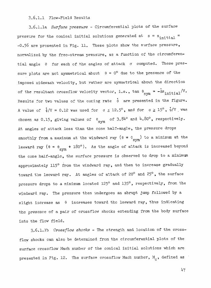
3.6.1.1 Flow-Field Results

3.6 .1.1a Surface pressure - Circumferential plots of the surface

pressure for the conical initial solutions generated at s = Sinitial =

-0.56 are presented in Fig. 11. These plots show the surface pressure,

normalized by the free-stream pressure, as a function of the circumferen-

tial angle 6 for each of the angles of attack a computed. These pres-

sure plots are not symmetrical about 0 = 00 due to the presence of the

imposed sidewash velocity, but rather are symmetrical about the direction

of the resultant crossflow velocity vector, i.e., tan 0sy m = initial/V.

Results for two values of the coning rate $ are presented in the figure.

A value of (/V = 0.12 was used for a < 12.50, and for a 150, ;/V was

chosen as 0.15, giving values of e of 3.840 and 4.800, respectively.sym

At angles of attack less than the cone half-angle, the pressure drops

smoothly from a maximum at the windward ray (e = m ) to a minimum at thesym

leeward ray (B = 0 + 180'). As the angle of attack is increased beyondsym

the cone half-angle, the surface pressure is observed to drop to a minimum

approximately 1150 from the windward ray, and then to increase gradually

toward the leeward ray. At angles of attack of 200 and 250, the surface

pressure drops to a minimum located 1250 and 1350, respectively, from the

windward ray. The pressure then undergoes an abrupt jump followed by a

slight increase as 0 increases toward the leeward ray, thus indicating

the presence of a pair of crossflow shocks extending from the body surface

into the flow field.

3,.6.1.lb Crossflow shocks - The strength and location of the cross-

flow shocks can also be determined from the circumferential plots of the

surface crossflow Mach number of the conical initial solutions which are

presented in Fig. 12. The surface crossflow Mach number, Mc, defined as

47

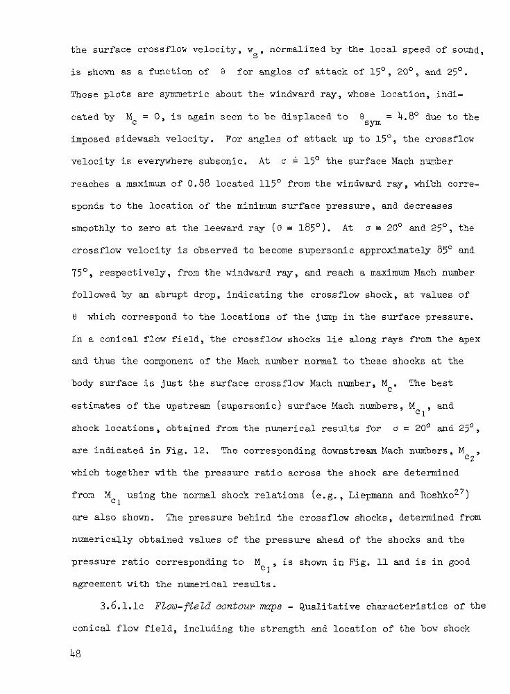
the surface crossflow velocity, ws, normalized by the local speed of sound,

is shown as a function of 6 for angles of attack of 150, 200, and 250.

These plots are symmetric about the windward ray, whose location, indi-

cated by M = O, is again seen to be displaced to 6 = 4.8 0 due to thec sym

imposed sidewash velocity. For angles of attack up to 150, the crossflow

velocity is everywhere subsonic. At a = 150 the surface Mach number

reaches a maximum of 0.88 located 1150 from the windward ray, whi'ch corre-

sponds to the location of the minimum surface pressure, and decreases

smoothly to zero at the leeward ray (e = 1850). At a = 200 and 250, the

crossflow velocity is observed to become supersonic approximately 850 and

750, respectively, from the windward ray, and reach a maximum Mach number

followed by an abrupt drop, indicating the crossflow shock, at values of

e which correspond to the locations of the jump in the surface pressure.

In a conical flow field, the crossflow shocks lie along rays from the apex

and thus the component of the Mach number normal to these shocks at the

body surface is just the surface crossflow Mach number, M . The best

estimates of the upstream (supersonic) surface Mach numbers, Mcl , and

shock locations, obtained from the numerical results for a = 200 and 250,

are indicated in Fig. 12. The corresponding downstream Mach numbers, Mc2,

which together with the pressure ratio across the shock are determined

from M using the normal shock relations (e.g., Liepmann and Roshko2 7 )

are also shown. The pressure behind the crossflow shocks, determined from

numerically obtained values of the pressure ahead of the shocks and the

pressure ratio corresponding to Ml , is shown in Fig. 11 and is in good

agreement with the numerical results.

3.6 .1.1c Flow-field contour maps - Qualitative characteristics of the

conical flow field, including the strength and location of the bow shock

48

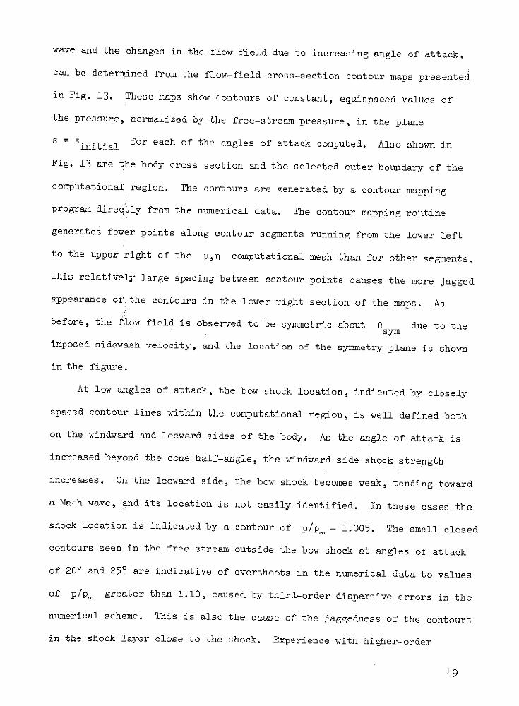
wave and the changes in the flow field due to increasing angle of attack,

can be determined from the flow-field cross-section contour maps presented

in Fig. 13. These maps show contours of constant, equispaced values of

the pressure, normalized by the free-stream pressure, in the plane

s = Sinitial for each of the angles of attack computed. Also shown in

Fig. 13 are the body cross section and the selected outer boundary of the

computational region. The contours are generated by a contour mapping

program directly from the numerical data. The contour mapping routine

generates fewer points along contour segments running from the lower left

to the upper right of the p,n computational mesh than for other segments.

This relatively large spacing between contour points causes the more jagged

appearance of.the contours in the lower right section of the maps. As

before, the flow field is observed to be symmetric about 6 due to thesym

imposed sidewash velocity, and the location of the symmetry plane is shown

in the figure.

At low angles of attack, the bow shock location, indicated by closely

spaced contour lines within the computational region, is well defined both

on the windward and leeward sides of the body. As the angle of attack is

increased beyond the cone half-angle, the windward side shock strength

increases. On the leeward side, the bow shock becomes weak, tending toward

a Mach wave, and its location is not easily identified. In these cases the

shock location is indicated by a contour of p/p. = 1.005. The small closed

contours seen in the free stream outside the bow shock at angles of attack

of 200 and 250 are indicative of overshoots in the numerical data to values

of p/pm greater than 1.10, caused by third-order dispersive errors in the

numerical scheme. This is also the cause of the jaggedness of the contours

in the shock layer close to the shock. Experience with higher-order

49

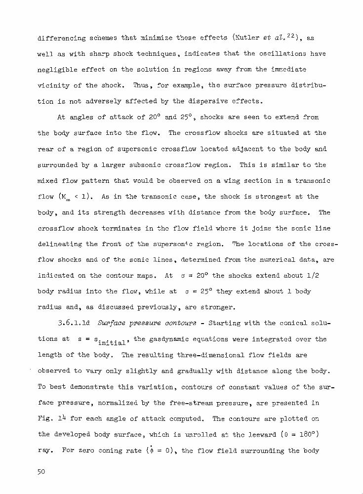
differencing schemes that minimize these effects (Kutler et aZ.2 2 ), as

well as with sharp shock techniques, indicates that the oscillations have

negligible effect on the solution in regions away from the immediate

vicinity of the shock. Thus, for example, the surface pressure distribu-

tion is not adversely affected by the dispersive effects.

At angles of attack of 200 and 250, shocks are seen to extend from

the body surface into the flow. The crossflow shocks are situated at the

rear of a region of supersonic crossflow located adjacent to the body and

surrounded by a larger subsonic crossflow region. This is similar to the

mixed flow pattern that would be observed on a wing section in a transonic

flow (M < 1). As in the transonic case, the shock is strongest at the

body, and its strength decreases with distance from the body surface. The

crossflow shock terminates in the flow field where it joins the sonic line

delineating the front of the supersonic region. The locations of the cross-

flow shocks and of the sonic lines, determined from the numerical data, are

indicated on the contour maps. At a = 200 the shocks extend about 1/2

body radius into the flow, while at a = 250 they extend about 1 body

radius and, as discussed previously, are stronger.

3.6.1.id Surface pressure contours - Starting with the conical solu-

tions at s = s.initial the gasdynamic equations were integrated over the

length of the body. The resulting three-dimensional flow fields are

observed to vary only slightly and gradually with distance along the body.

To best demonstrate this variation, contours of constant values of the sur-

face pressure, normalized by the free-stream pressure, are presented in

Fig. 14 for each angle of attack computed. The contours are plotted on

the developed body surface, which is unrolled at the leeward (6 = 1800)

ray. For zero coning rate ($ = 0), the flow field surrounding the body

50

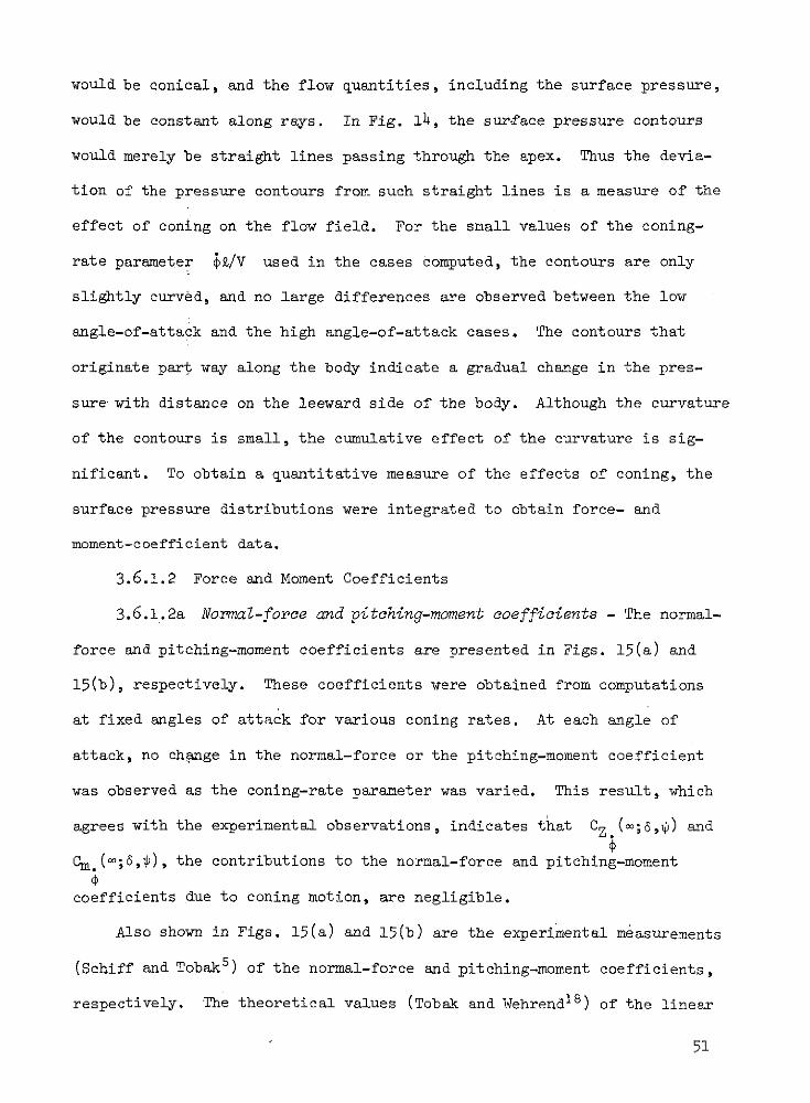
would be conical, and the flow quantities, including the surface pressure,

would be constant along rays. In Fig. 14, the surface pressure contours

would merely be straight lines passing through the apex. Thus the devia-

tion of the pressure contours from such straight lines is a measure of the

effect of coning on the flow field. For the small values of the coning-

rate parameter £/V used in the cases computed, the contours are only

slightly curved, and no large differences are observed between the low

angle-of-attack and the high angle-of-attack cases. The contours that

originate part way along the body indicate a gradual change in the pres-

sure with distance on the leeward side of the body. Although the curvature

of the contours is small, the cumulative effect of the curvature is sig-

nificant. To obtain a quantitative measure of the effects of coning, the

surface pressure distributions were integrated to obtain force- and

moment-coefficient data.

3.6.1.2 Force and Moment Coefficients

3.6 .1.2a Normal-force and pitching-moment coefficients - The normal-

force and pitching-moment coefficients are presented in Figs. 15(a) and

15(b), respectively. These coefficients were obtained from computations

at fixed angles of attack for various coning rates. At each angle of

attack, no change in the normal-force or the pitching-moment coefficient

was observed as the coning-rate parameter was varied. This result, which

agrees with the experimental observations, indicates that Cz.(m;6,) and

Cm.(m;6,*), the contributions to the normal-force and pitching-moment

coefficients due to coning motion, are negligible.

Also shown in Figs. 15(a) and 15(b) are the experimental measurements

(Schiff and Tobak 5) of the normal-force and pitching-moment coefficients,

respectively. The theoretical values (Tobak and Wehrend'8 ) of the linear

51

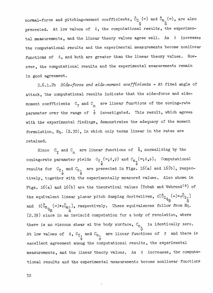
normal-force and pitching-moment coefficients, CZ (m) and m (H), are also& &i

presented. At low values of 6, the computational results, the experimen-

tal measurements, and the linear theory values agree well. As 6 increases

the computational results and the experimental measurements become nonlinear

functions of 6, and both are greater than the linear theory values. How-

ever, the computational results and the experimental measurements remain

in good agreement.

3.6.1.2b Side-force and side-moment coefficients - At fixed angle of

attack, the computational results indicate that the side-force and side-

moment coefficients Cy and Cn are linear functions of the coning-rate

parameter over the range of 4 investigated. This result, which agrees

with the experimental findings, demonstrates the adequacy of the moment

formulation, Eq. (2.30), in which only terms linear in the rates are

retained.

Since Cy and Cn are linear functions of , normalizing by the

coning-rate parameter yields Cy.(-;6,P) and Cn. (;6,). Computational

results for Cy. and Cn. are presented in Figs. 16 (a) and 16(b), respec-

tively, together with the experimentally measured values. Also shown in

Figs. 16 (a) and 16(b) are the theoretical values (Tobak and Wehrendl8) of

the equivalent linear planar pitch damping derivatives, 6[IZ ()+Y Z.]

and 6[Im ()+yCm.], respectively. These equivalences follow from Eq.

qB &(2.39) since in an inviscid computation for a body of revolution, where

there is no viscous shear at the body surface, Cn is identically zero.

At low values of 6, Cy. and Cn. are linear functions of 6 and there is

excellent agreement among the computational results, the experimental

measurements, and the linear theory values. As 6 increases, the computa-

tional results and the experimental measurements become nonlinear functions

52

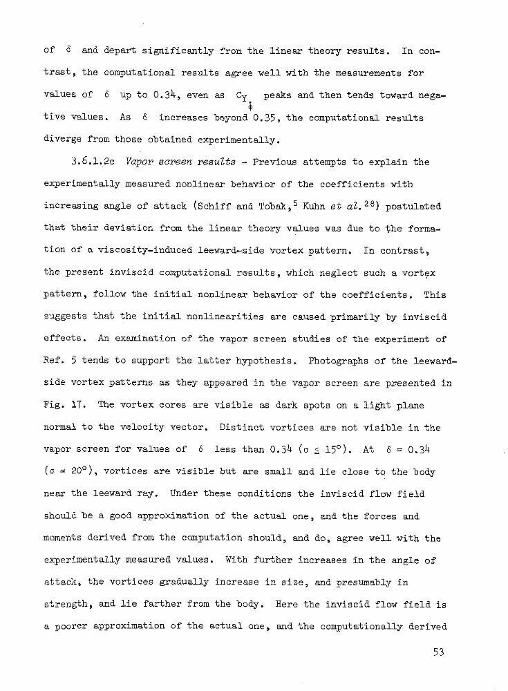
of 6 and depart significantly from the linear theory results. In con-

trast, the computational results agree well with the measurements for

values of 6 up to 0.34, even as Cy peaks and then tends toward nega-

tive values. As 6 increases beyond 0.35, the computational results

diverge from those obtained experimentally.

3.6 .1.2c Vapor screen results - Previous attempts to explain the

experimentally measured nonlinear behavior of the coefficients with

increasing angle of attack (Schiff and Tobak,5 Kuhn et al. 2 8) postulated

that their deviation from the linear theory values was due to the forma-

tion of a viscosity-induced leeward-side vortex pattern. In contrast,

the present inviscid computational results, which neglect such a vortex

pattern, follow the initial nonlinear behavior of the coefficients. This

suggests that the initial nonlinearities are caused primarily by inviscid

effects. An examination of the vapor screen studies of the experiment of

Ref. 5 tends to support the latter hypothesis. Photographs of the leeward-

side vortex patterns as they appeared in the vapor screen are presented in

Fig. 17. The vortex cores are visible as dark spots on a light plane

normal to the velocity vector. Distinct vortices are not visible in the

vapor screen for values of 6 less than 0.34 (a S 150). At 6 = 0.34

(a = 200), vortices are visible but are small and lie close to the body

near the leeward ray. Under these conditions the inviscid flow field

should be a good approximation of the actual one, and the forces and

moments derived from the computation should, and do, agree well with the

experimentally measured values. With further increases in the angle of

attack, the vortices gradually increase in size, and presumably in

strength, and lie farther from the body. Here the inviscid flow field is

a poorer approximation of the actual one, and the computationally derived

53

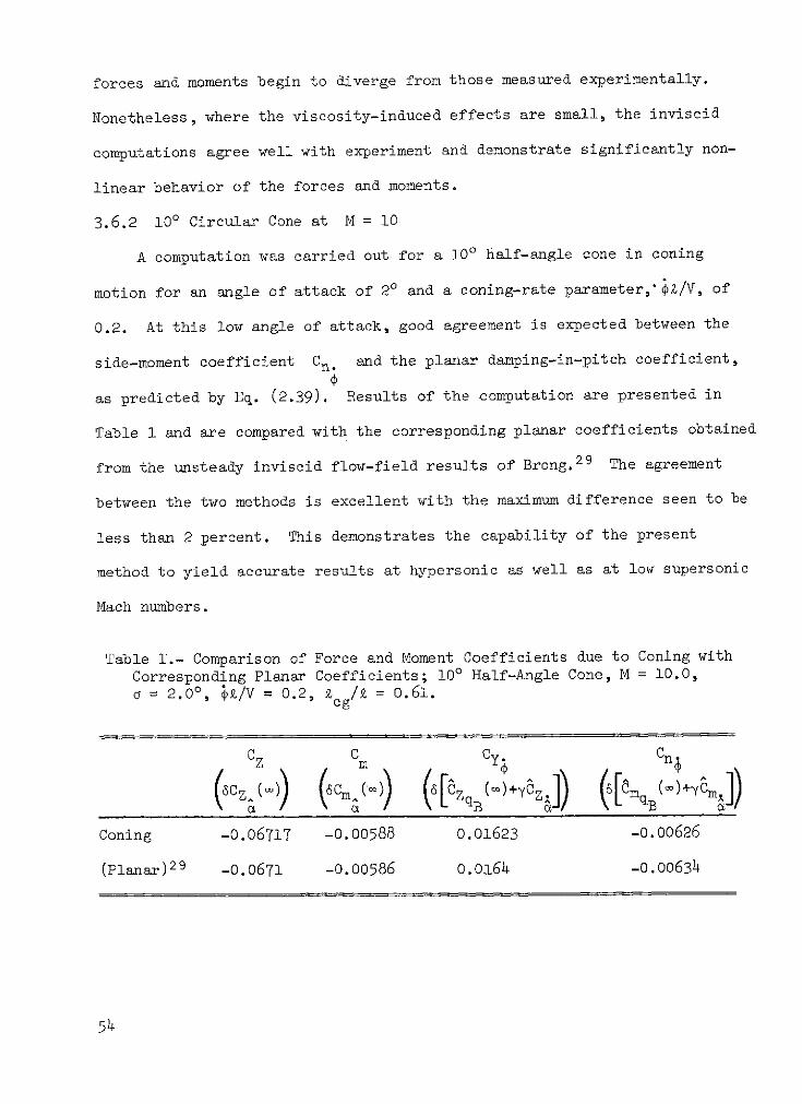
forces and moments begin to diverge from those measured experimentally.

Nonetheless, where the viscosity-induced effects are small, the inviscid

computations agree well with experiment and demonstrate significantly non-

linear behavior of the forces and moments.

3.6.2 100 Circular Cone at M = 10

A computation was carried out for a 100 half-angle cone in coning

motion for an angle of attack of 20 and a coning-rate parameter,'$Z/V, of

0.2. At this low angle of attack, good agreement is expected between the

side-moment coefficient Cn. and the planar damping-in-pitch coefficient,

as predicted by Eq. (2.39). Results of the computation are presented in

Table 1 and are compared with the corresponding planar coefficients obtained

from the unsteady inviscid flow-field results of Brong.2 9 The agreement

between the two methods is excellent with the maximum difference seen to be

less than 2 percent. This demonstrates the capability of the present

method to yield accurate results at hypersonic as well as at low supersonic

Mach numbers.

Table I.- Comparison of Force and Moment Coefficients due to Coning with

Corresponding Planar Coefficients; 100 Half-Angle Cone, M = 10.0,

a = 2.00, $£/V = 0.2, acg / = 0.61.

CZ Cm Cy Cn

(6CZ1 )) (Cm()) (6[ZqBI+(m ([mq (m)+ym])

Coning -0.06717 -0.00588 0.01623 -0.00626

(Planar)2 9 -0.0671 -0.00586 0.0164 -0.00634

54

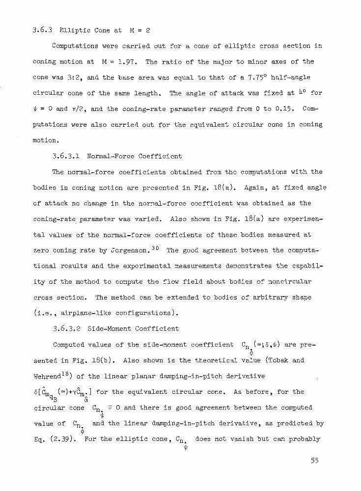
3.6.3 Elliptic Cone at M = 2

Computations were carried out for a cone of elliptic cross section in

coning motion at M = 1.97. The ratio of the major to minor axes of the

cone was 3:2, and the base area was equal to that of a 7.750 half-angle

circular cone of the same length. The angle of attack was fixed at 40 for

= 0 and 7/2, and the coning-rate parameter ranged from 0 to 0.15. Com-

putations were also carried out for the equivalent circular cone in coning

motion.

3.6.3.1 Normal-Force Coefficient

The normal-force coefficients obtained from the computations with the

bodies in coning motion are presented in Fig. 18(a). Again, at fixed angle

of attack no change in the normal-force coefficient was obtained as the

coning-rate parameter was varied. Also shown in Fig. 18(a) are experimen-

tal values of the normal-force coefficients of these bodies measured at

zero coning rate by Jorgenson.30 The good agreement between the computa-

tional results and the experimental measurements demonstrates the capabil-

ity of the method to compute the flow field about bodies of noncircular

cross section. The method can be extended to bodies of arbitrary shape

(i.e., airplane-like configurations).

3.6.3.2 Side-Moment Coefficient

Computed values of the side-moment coefficient Cn (c;6,5) are pre-

sented in Fig. 18(b). Also shown is the theoretical value (Tobak and

Wehrend1 8) of the linear planar damping-in-pitch derivative

6[ C ()+yCm.] for the equivalent circular cone. As before, for the

circular cone Cn. E 0 and there is good agreement between the computed

value of Cn. and the linear damping-in-pitch derivative, as predicted by

Eq. (2.39). For the elliptic cone, Cn. does not vanish but can probably

55

be neglected in comparison with Cn.. Under these conditions, Eq. (2.33)

indicates that Cn.(m;6,/2) = 6[iCm () + yCm.] and

Cn.(0;6,0) = 6[Cn (0") - yCn]. These are the planar damping coefficientsB B

for oscillations in the directions indicated by the double-headed arrows

in Fig. 18(b). The computational results confirm the expectation that

oscillations parallel to the major axis of the elliptical cone should be

less strongly damped than those parallel to the minor axis.

4. CONCLUDING REMARKS

Concepts from the theory of functionals have been applied to develop

nonlinear formulations of the aerodynamic force and moment systems acting

on bodies in arbitrary, slowly varying, large-amplitude motions. The anal-

ysis, which proceeds formally once the functional dependence of the aero-

dynamic reactions upon the motion variables has been established, ensures

the inclusion of all pertinent aerodynamic terms within the resulting

formulations. The results confirm formally the intuitive notion that the

instantaneous reactions on a body in an arbitrary motion can be compounded

of the contributions from several characteristic motions: a steady motion

with the instantaneous large values of the motion variables held fixed,

and suitable perturbations about the steady motion.

The analysis indicates that coning, where the nose of the body

describes a circle around the velocity vector, characterizes the nonplanar

nature of a general motion. With this motivation, a numerical method was

developed for computing the inviscid flow field surrounding a body in con-

ing motion. Computations carried out for circular cones in coning motion

both at low supersonic and hypersonic Mach numbers confirm the adequacy of

a linear formulation at low angles of attack. At larger angles of attack,

56

however, the forces and moments become nonlinear functions of the angle of

attack. Computational results for the reactions on-the circular cone at

the higher angles of attack agreed well with experimental measurements

within the range of variables investigated. This indicates that the ini-

tial nonlinear behavior of the aerodynamic forces and moments is governed

primarily by the inviscid flow and not, as previously postulated, by the

viscosity-induced leeward-side vortices.

Ames Research Center

National Aeronautics and Space Administration

Moffett Field, Calif., 94035,,August 24, 1973

57

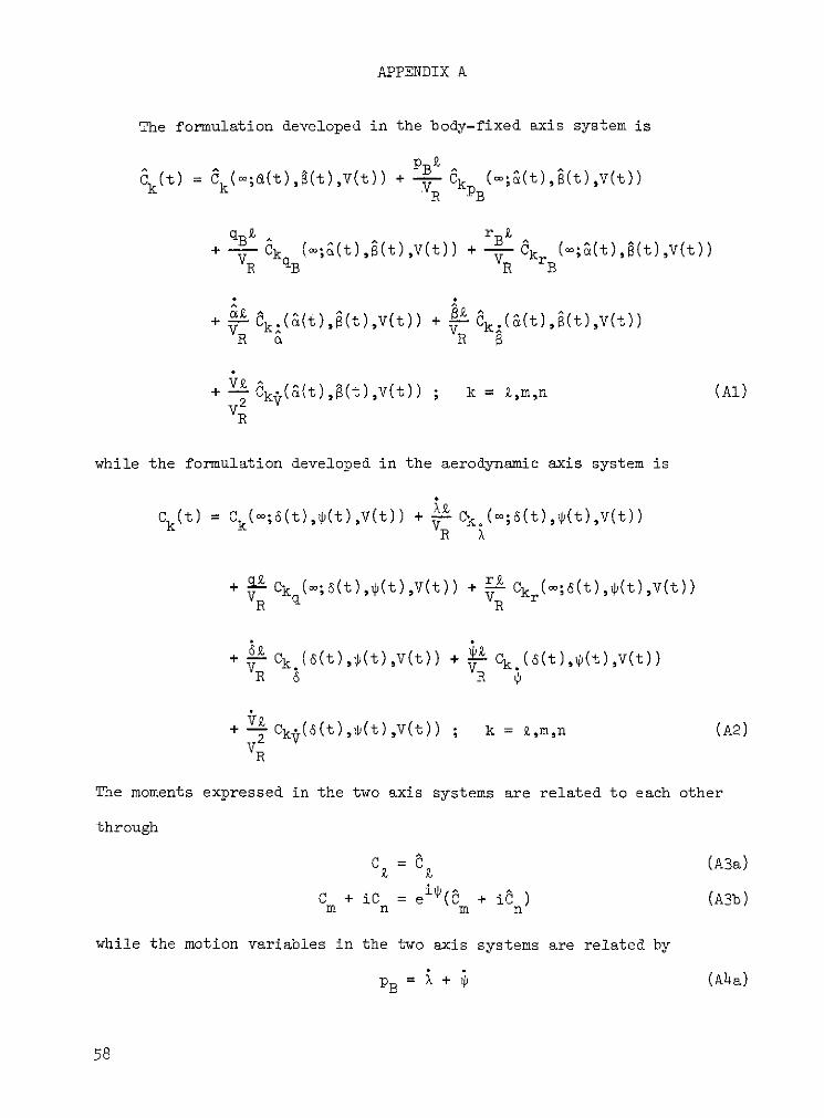
APPENDIX A

The formulation developed in the body-fixed axis system is

pBRCk(t) = Ck(;;(t),(t),V(t)) + - CkPB(m;&(t),B(t),V(t))

qB ^ rB

+ ^BZ ak + (t) ,V)R B R B

R a R B

+ k = z,m,n (Al)

R

while the formulation developed in the aerodynamic axis system is

Ck(t) = Ck(;6(t)(t),V(t)) + - Ck.(;(t),4(t),V(t))R X

+ - Ck (;(t)(t),(t,V(t)) + - Ckr (;6(t),(t),v(t))VR R

+ 6 Ck.(6(t),(t),V(t)) + - Ck.(6(t),(t),V(t))R 6 R

+ Ck (6(t),(t),V(t)) ; k = k,m,n (A2)VR

The moments expressed in the two axis systems are related to each other

through

C = C (A3a)

C + iC= e"i(C + i ) (A3b)m n m n

while the motion variables in the two axis systems are related by

PB = + (Aha)

58

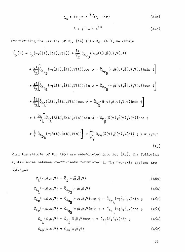
B + irB = e (q + ir) (A4b)

& + i = 6 ei (A4c)

Substituting the results of Eq. (A4) into Eq. (Al), we obtain

C (t) = k( ;&(t),(t)(t) t)) + kPB(^

+ (;(t),(t),V(t))cos - k (;(t),(t),V(t))sin

+ k (";a(t),R(t),v(t))sin 4 + kr (m;&(t),(t),v(t))cos 4]

+ -k.((t),(t),V(t))cos + k((t),(t),V(t))sin p]

+ 6 -Ck.(&(t),(t),V(t))sin i + Ck.(c(t),R(t),V(t))cos )

+ ~ CkPB (&;(t),(t),V(t)) + Cki(^(t),+(t),V(t)) ; k = ,m,nVR

(A5)

When the results of Eq. (A5) are substituted into Eq. (A3), the following

equivalences between coefficients formulated in the two-axis systems are

obtained:

c (m;6,,v) = R (c;a, ,v) (A6a)

C a(m;6,4,V) = p (B ;&,B,V) (A6b)X

C (=;6,4,V) = B(;&,8,V)cos i - CrB(c;&,,V)sin 4 (A6c)

C r( ;6,*,v) = B(o ;&,8,V)sin ^ + OArB(m ;&,,v)cos p (A6d)

c, (6,4,v) = C .(&,,v)cos 4 + ig.(&,8,V)sin p (A6e)

cR (6,4,v) = (,,V ) (A6f)

59

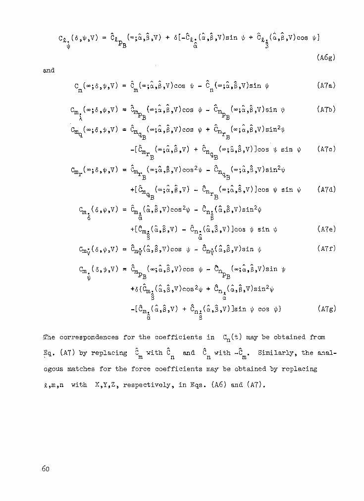
aC.(a,(,V) = -C (;&a,B,V) + a[-C.(a,,)sin p + C.(a,a,V)cos i]

(A6g)

and

C m(;6'',v) = c m( = ; ,~, ' V )cos - Cn(m;&,,V)sin i (A7a)

Cm (i6,p,V) = B(M;B,;B,V)cos - nB(;a';,V)sin (ATb)

Cm (m;6,i,V) = Cm B(C;a, ,V)cos + CnrB(m;a,B,V)sin2p

-4mrB (;&,,V) + Cn B(;&,8,V)]cos p sin p (A7c)

Cmr(m;6,*,V) = mr B( ;&,,V)cos2 - C B(o;&,^,V)sin 2,

+[m n(;aBV) - i (-;&,,V)]cos i sin p (A7d)B B

Cm.(6,4,V) = cm.(,,V)cos2 -,n.(,,V)sin 2

+[Iim.(a,,V) - Cn.(&,,V)]cos , sin , (A7e)

Cm4 (6,p,v) = i(a,LV)os i - Cn(&, ,v)sin p (ATr)

a

cm.(6,pv) = - PB ,V)sin

+6{C,.(a,;,V)cos2 + Cn (a,,V)sin2p

-[Cm.(a,,v) + Cn.(a, ,V)lsin i cos }) (A7g)

nThe correspondences for the coefficients in Cn(t) may be obtained from

Eq. (AT) by replacing C with C and C with -C . Similarly, the anal-m n n m

ogous matches for the force coefficients may be obtained by replacing

k,m,n with X,Y,Z, respectively, in Eqs. (A6) and (A7).

60

REFERENCES

1Etkin, B., Dynamics of FZight, John Wiley & Sons, New York, 1959.

2Nicolaides, J. D., Eikenberry, R. S., Ingram, C. W., and Kryvoruka,

J. K., "Non-Linear Aerodynamic Characteristics of Re-Entry Configurations

with Aerodynamic and Mass Asymmetries," AIAA Paper 69-867, 1969.

31ngram, C. W., "An Approximate Solution for the Nonlinear Differential

Equation for the Complex Angle of Attack of a Symmetrical Missile," AFATL-

TR-68-71, Air Force Armament Laboratory, Eglin Air Force Base, Florida,

June 1968.

41yengar, S., "Experimental Damping-in-Pitch of Two Slender Cones at

Mach 2 and Incidences Up to 300," LTR-UA-19, National Research Council,

Ottawa, Canada, Jan. 1968.

5Schiff, L. B., and Tobak, M., "Results from a New Wind-Tunnel Appara-

tus for Studying Coning and Spinning Motions of Bodies of Revolution," AIAA

Journal, Vol. 8, No. 11, pp. 1953-1957, Nov. 1970.

6Murphy, C. H., "Free Flight Motion of Symmetric Missiles," Rept.

BRL-1216, Ballistic Research Lab., Aberdeen Proving Ground, Maryland, July

1963.

7Tobak, M., and Pearson, W. E., "A Study of Nonlinear Longitudinal

Dynamic Stability," TR R-209, NASA, Sept. 1964.

8Tobak, M., Schiff, L. B., and Peterson, V. L., "Aerodynamics of

Bodies of Revolution in Coning Motion," AIAA Journal, Vol. 7, No. 1,

pp. 95-99, Jan. 1969.

9Levy, L. L., Jr., and Tobak, M., "Nonlinear Aerodynamics of Bodies

of Revolution in Free Flight," AIAA Journal, Vol. 8, No. 12, pp. 2168-2171,

Dec. 1970.

61

10Tobak, M., and Schiff, L. B., "A Nonlinear Aerodynamic Moment Formu-

lation and Its Implications for Dynamic Stability Testing," AIAA Paper

71-275, 1971.

1 1MacCormack, R. W., "The Effect of Viscosity in Hypervelocity Impact

Cratering," AIAA Paper 69-364, 1969.

1 2Kutler, P., and Lomax, H., "Shock-Capturing, Finite-Difference

Approach to Supersonic Flows," Journal of Spacecraft and Rockets, Vol. 8,

No. 12, pp. 1175-1182, Dec. 1971.

13Volterra, V., Theory of Functionals and of Integral and Integro-

Differential Equations, Dover Publications, Inc., New York, 1959.

14Regan, F. J., and Horanoff, E. V., "Wind Tunnel Magnus Measurements

at the Naval Ordnance Laboratory," AIAA Paper 66-753, 1966.

1 5platou, A. S., and Sternberg, J., "The Magnus Characteristics of a

30 mm Aircraft Bullet," Rept. 994, Ballistic Research Lab., Aberdeen Prov-

ing Ground, Maryland, 1954.

1 6platou, A. S., "The Magnus Force on a Short Body at Supersonic

Speeds," Rept. 1062, Ballistic Research Lab., Aberdeen Proving Ground,

Maryland, 1959.

17Sedney, R., "Laminar Boundary Layer on a Spinning Cone at Small

Angles of Attack in a Supersonic Flow," Journal of the Aeronautical

Sciences, Vol. 24, No. 6, pp. 430-436, June 1957.

18Tobak, M., and Wehrend, W. R., "Stability Derivatives of Cones at

Supersonic Speeds," TN 3788, NACA, 1956.

1 9Rakich, J. V., and Kutler, P., "Comparison of Characteristic and

Shock-Capturing Methods with Application to the Space Shuttle," AIAA

Paper 72-191, 1972.

2 0Richtmyer, R. D., and Morton, R. W., Difference Methods for Initial-

Value Problems, Interscience, New York, pp. 304, 360-365, 1967.

62

2 1Abbett, M. J., "Boundary Condition Computational Procedures for

Inviscid Supersonic Steady Flow Field Calculations," Final Rept. 71-41,

Aerotherm Corp., Mountain View, California, Nov. 1971.

2 2Kutler, P., Lomax, H., and Warming, R. F., "Computation of Space

Shuttle Flow Fields Using Noncentered Finite-Difference Schemes," AIAA

Paper 72-193, 1972.

2 3Babenko, K. I., Voskresenskiy, G. P., Lyubimov, A. N., and Rusanov,

V. V., "Three-Dimensional Flow of Ideal Gas Past Smooth Bodies," TT F-380,

NASA, April 1966.

24Rakich, J. V., "Three-Dimensional Flow Calculations by the Method

of Characteristics," AIAA Journal, Vol. 5, No. 10, pp. 1906-1908, Oct. 1967.

2 5Ferri, A., "Supersonic Flow Around Circular Cones at Angles of

Attack," Rept. 1045, NACA, 1951.

2 6Allen, H. J., and Perkins, E. W., "A Study of the Effects of Vis-

cosity on Flow Over Slender Inclined Bodies of Revolution," Rept. 1048,

NACA, 1951.

2 7Liepmann, H. W., and Roshko, A., EZements of Gasdynamics, John

Wiley & Sons, New York, pp. 57-61, 1957.

2 8Kuhn, G. D., Spangler, S. B., and Nielsen, J. N., "Theoretical

Analysis of Vortex Shedding from Bodies of Revolution in Coning Motion,"

AIAA Journal, Vol. 9, No. 5, pp. 784-790, May 1971.

2 9Brong, E. A., "The Unsteady Flow Field About a Right Circular Cone

in Unsteady Flight," FDL-TR-64-148, Flight Dynamics Lab., Wright-Patterson

Air Force Base, Ohio, Jan. 1967.

30Jorgenson, L. H., "Elliptic Cones Alone and With Wings at Super-

sonic Speeds," TN 4045, NACA, 1957.

63

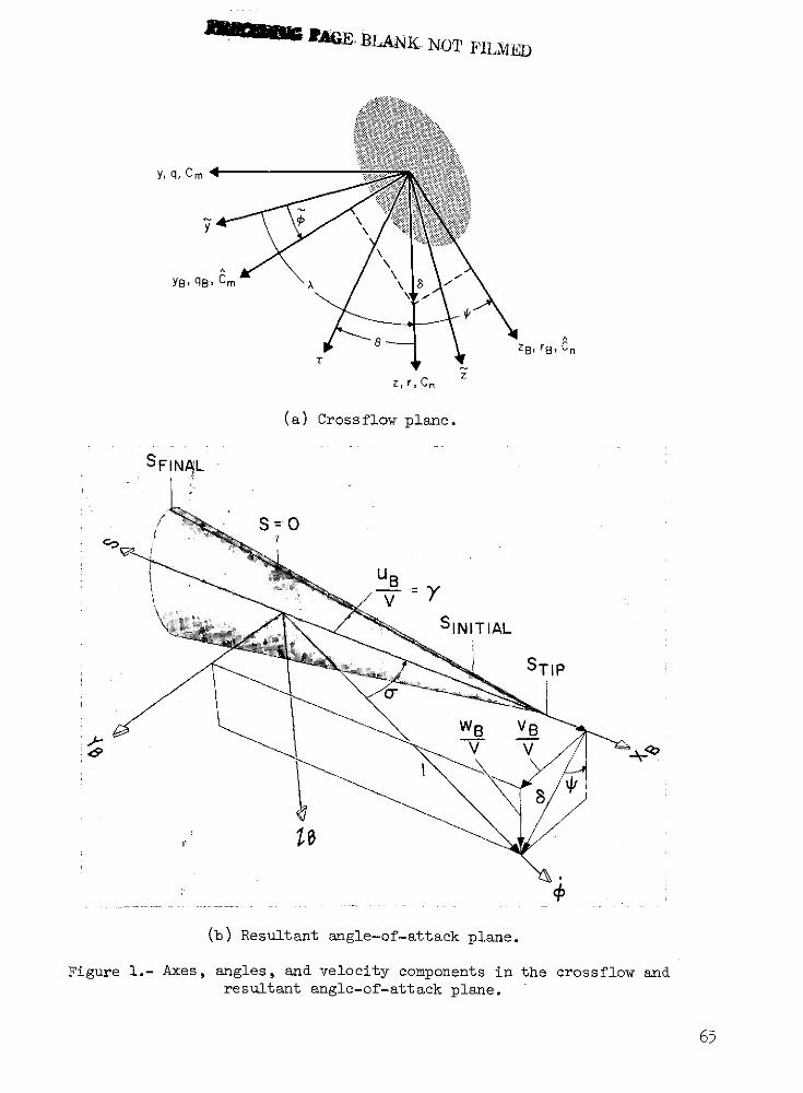
RAGE BLANK. NOT FILMED

y, q, Cm 4

Y9, 48, Cm X \ /

zB, rB , Cn

z, r, Cn

(a) Crossflow plane.

SFINAL

S=O

*U/V

SINITIAL

STIP

w B VBV V

(b) Resultant angle-of-attack plane.

Figure 1.- Axes, angles, and velocity components in the crossflow andresultant angle-of-attack plane.

65

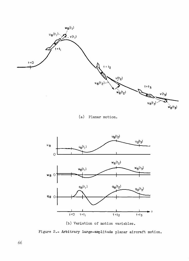
WB(tI)

UB(t) v (t )

t=Ot = t2

v (t 2)

t--o3

ug(tt 3)

(a) Planar motion.

ug(t 2)

WB(t2)

qB(t,) q(t2)

w8 O

qB 0--

I I I I s t

t=O t=t I t=t2 tt3

(b) Variation of motion variables.

Figure 2.- Arbitrary large-amplitude planar aircraft motion.

66

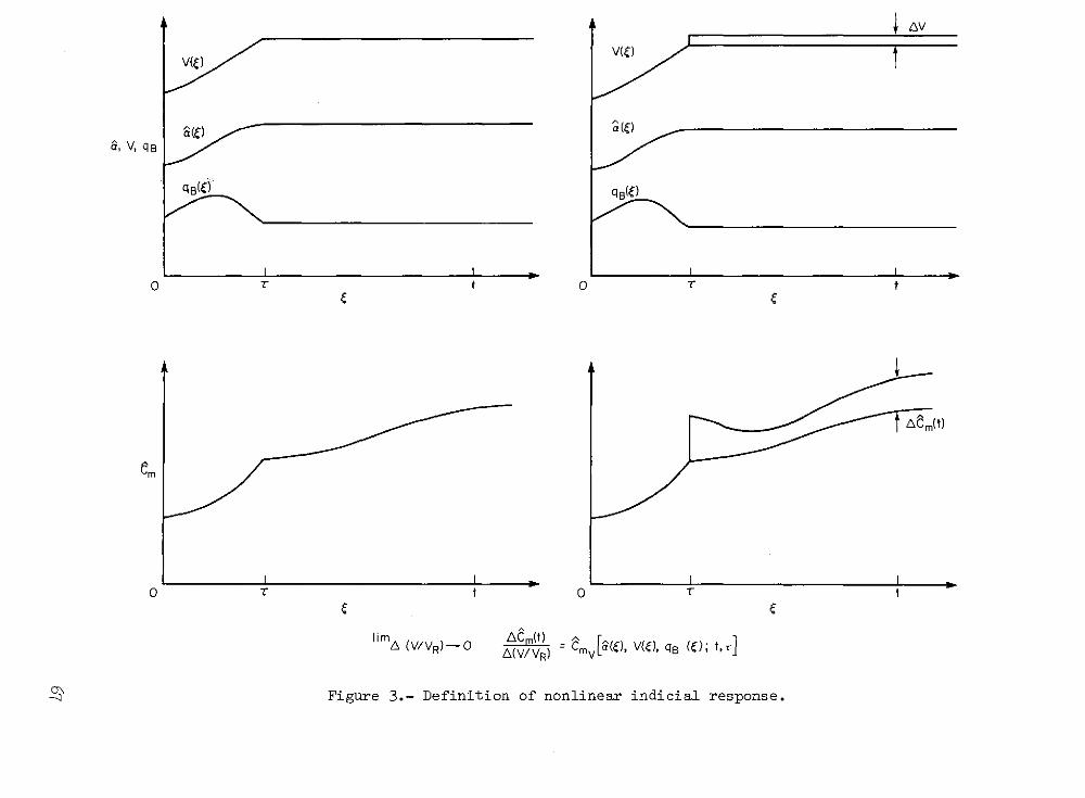
a, V, qB

_ ______ I -

0 T t 0T t

lim m (t)

S(V/VR)-0 A(V/VR) Cm[('), V(,), q 8 (C); t,r

Figure 3.- Definition of nonlinear indicial response.

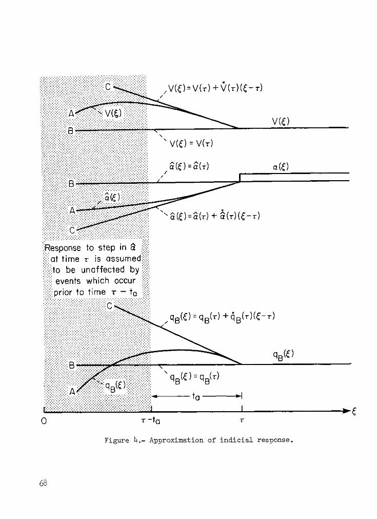
V (()A

(T)

:Response to step in :at time r is assumed....to be unaffected byevents which occur

prior to time r - ta

9s(iiqB BB()+ B()( - )

Ata (

0 r -to r

Figure 4.- Approximation of indicial response.

68

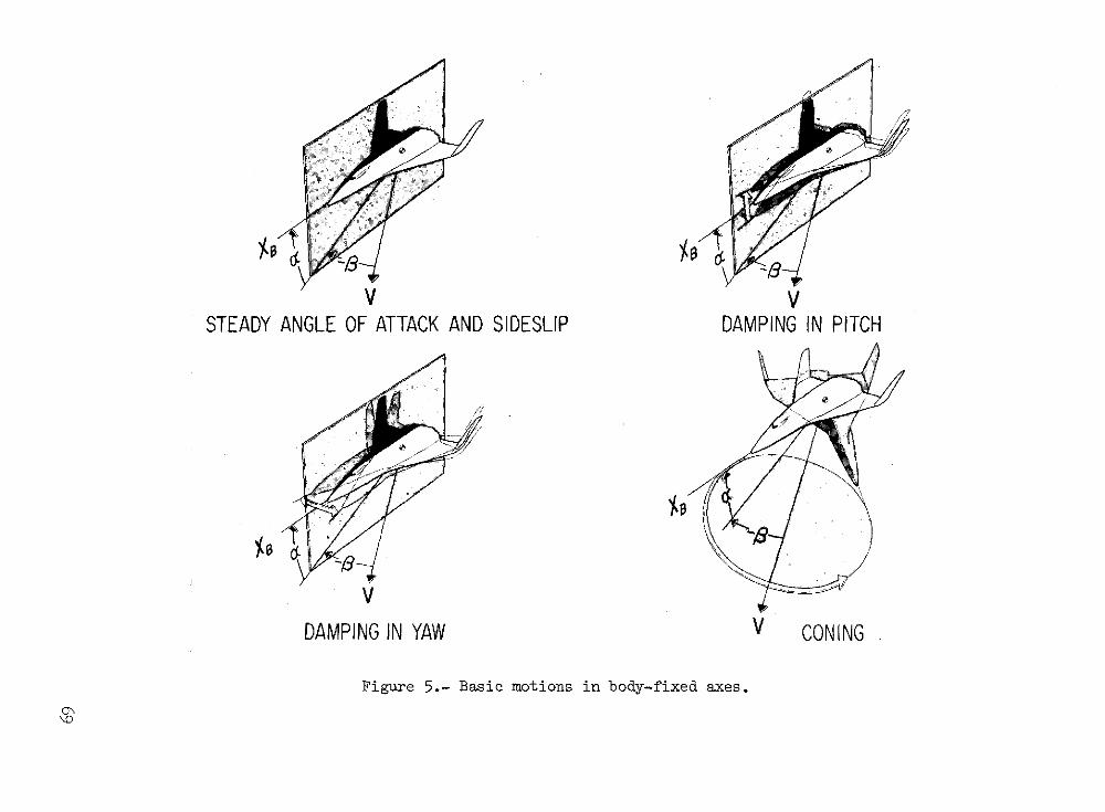
V VSTEADY ANGLE OF ATTACK AND SIDESLIP DAMPING IN PITCH

DAMPING IN YAW V CONING

Figure 5.- Basic motions in body-fixed axes.

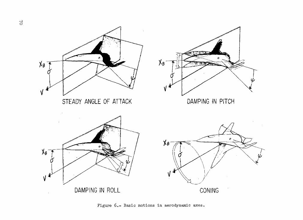
0

STEADY ANGLE OF ATTACK DAMPING IN PITCH

DAMPING IN ROLL CONING

Figure 6.- Basic motions in aerodynamic axes.

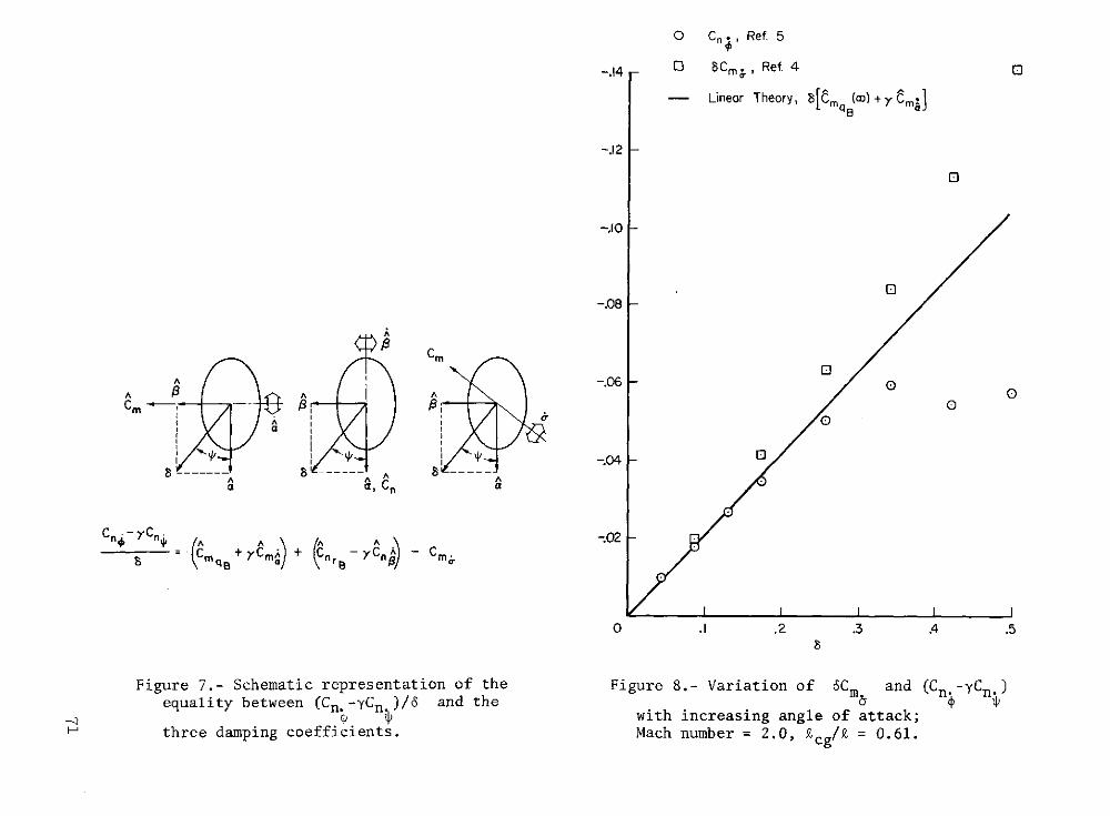
0 Cn., Ref. 5

-.14 O 8Cm , Ref. 4 [

- Linear Theory, 8[CmB) + Y Cm]

-.12

0

-.10

0-.08

A

Cm

A -. 06 0A ( A A 0

A 0

8 a, c8 -

(mq ~ + (enr-yn1 - Cm2

0 .1 .2 .3 .4 .5

Figure 7.- Schematic representation of the Figure 8.- Variation of 6Cm and (Cn. -Cn)equality between (Cn -yCn )1 6 and the 4

_, with increasing angle of attack;Hthree damping coefficients. Mach number = 2.0, cg/A = 0.61.

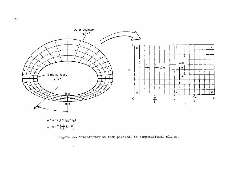
Outer boundary,Tob(8, S)

Ia f e

c d

Body surface,

rb(8, s)

bd b c d

Or 3r 27r2 2

= (T - rb) / (Tob- Tb)

S= tan-I(L tan 8)

Figure 9.- Transformation from physical to computational planes.

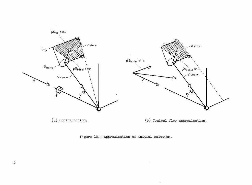
Stip sino-

S:tip ,-V sin cr - V sin -

\ 1Sinitial sina

Sinitil ' -S itia sSnitial sjn \

VC -V Cos 0

V\ V

(a) Coning motion. (b) Conical flow approximation.

Figure 10.- Approximation of initial solution.

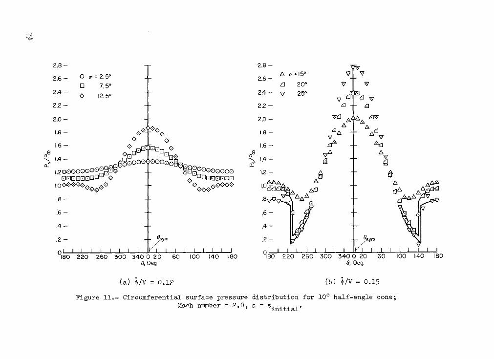
2.8 - 2.8 -

A -=15 0 V V2.6- O cr= 2.50 - 2.6 -

O 7.50 6 200 V V2.4 - 0 12.50 2.4- V 250

2.2 - - 2.2 - 4 n ,

2.0- -- 2.0- V A AA.8 - 1.8 -

V 71.6 - 1.6- 4A Ad

l A A

.21.0- -

.8- -- .8 --

1.4 - - 1.4 - -

.8- .. A

.6- .6-

.4- .4-

.2- -9sym .2 - S -/sym

0 1 I i I I I I I i I I I I I i o l I I 1i 1i 1 1 1I I I I I I I I180 220 260 300 340 0 20 60 100 140 180 180 220 260 300 340 0 20 60 100 140 180

8, Deg 8, Deg

(a) ;/V = 0.12 (b) ;/V = 0.15

Figure 11.- Circumferential surface pressure distribution for 100 half-angle cone;Mach number = 2.0, s = s.initia.initial'

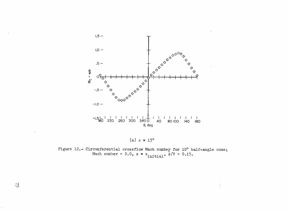
1.5 -

1.0 -

.5 - 0

-1.0 - -

80 220 260 300 340 0 40 80100 140 1808, deg

(a) a = 150

Figure 12.- Circumferential crossflow Mach number for 100 half-angle cone;Mach number = 2.0, s = Sinitial' 4/V = 0.15.

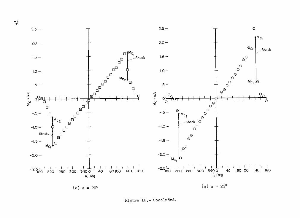
2.5 - -- 2.5 - O

McI

2.0 - -- 2.0 -

O0 -Shock

1.5 - [ -Shock 1.5- 0 O

1.0 - - 1.0 - 0O o

I M 00- .5 O MC2

% 0 -jShck 0.5

.5 - 3 .5 - 0

k0 0-. 5 M- 0 0 01 02

MC2 0 ,-Shock O

0 C0

-1.5 - -1.5 - 0

-2.0 - -2.0 -

McI

2.5 I I I I I I I I 2.5 L I I I I i i I I I I I I I

180 220 260 300 340 0 40 80100 140 180 180 220 260 300 3400 40 80 100 140 180

8, Deg 8, Deg

(b) a = 200 (c) a = 250

Figure 12.- Concluded.

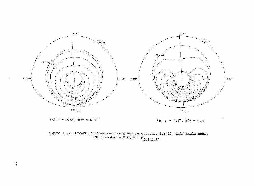
OuterOue

bundry bo--~undary

P/PPa

U.

P/P, 1.055

=90 827090

1.20

(a) a = 2.50, $/V = 0.12 (b) = 7.50, $/V = 0.12

Figure 13.- Flow-field cross section pressure contours for 100 half-angle cone;Mach number = 2,0, s = s.. lInitial"

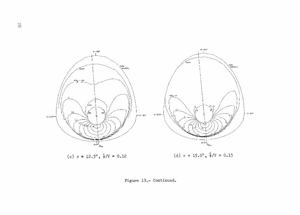
88 180*

cu Outerter

8 =900°

=270

I 3

(c) a = 12.50, $/V = 0.12 (d) a = 15.00, $/V = 0.15

Figure 13.- Continued.

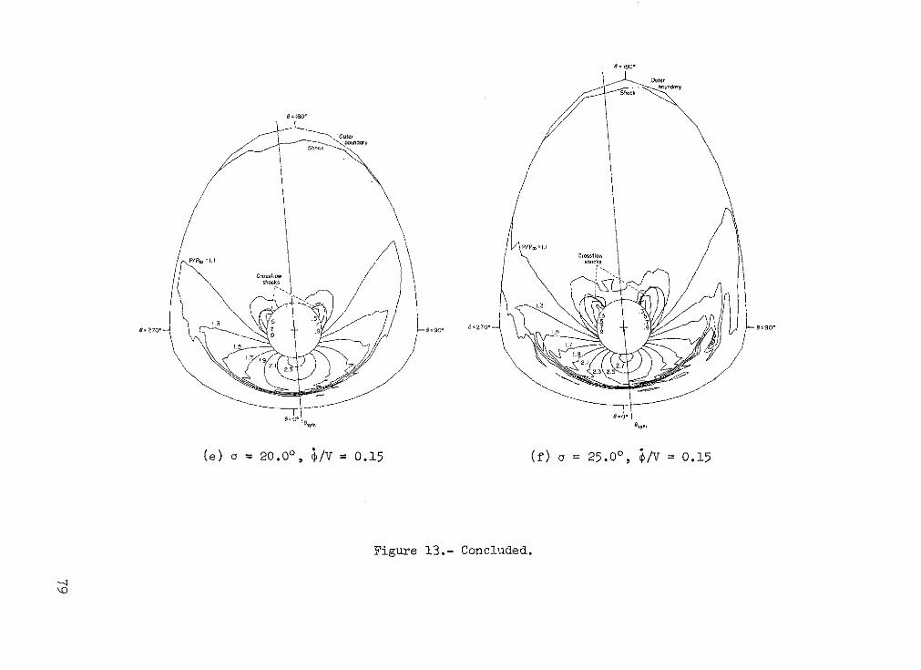
8180Outerbourdry

s Shock

p/p,, 1.1

hock

L3 .5 :5 .7= 270'7 8 =270- 7.

9 61.5

1 915 1.7

23 2.3 2.5

(e) a = 20.0 ° , ;/V= 0.15 (f) a = 25.00, /v = 0.15

Figure 13.- Concluded.

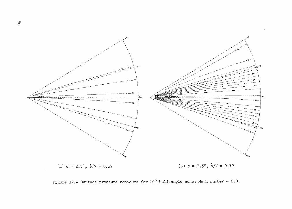
Co

1.300

O

1535

tA5

G0q 1190

(a) a = 2.5', /v = 0.12 (b) a = 7.5' , $/V = 0.12

Figure 14. Surface pressure contours for 100 half-angle cone; Mach number = 2.0.

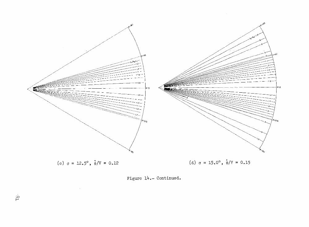
118

o 9

110 a

(c) a = 12.50, ;/V = 0.12 (a) a = 15.00, /V = 0.15

Figure 14.- Continued.

H-1

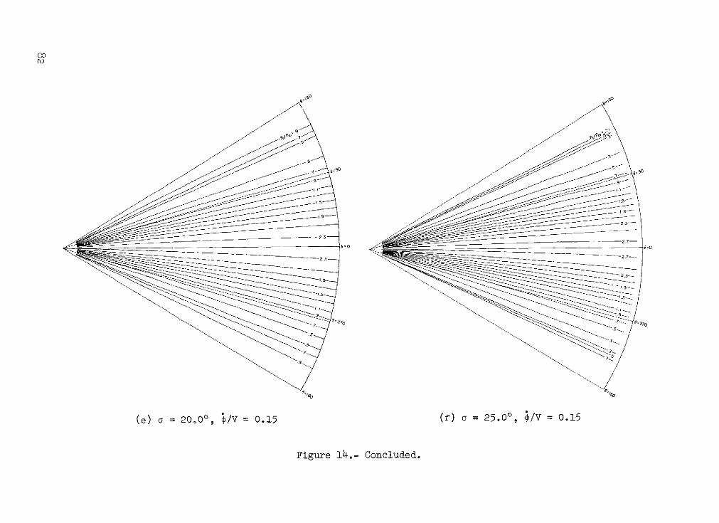
Co

2-

18-0

3~.9

9-

ae 20.0', ;/V 0.15 f)o=25.0', $/V =0.15

Figure 14, Concluded.

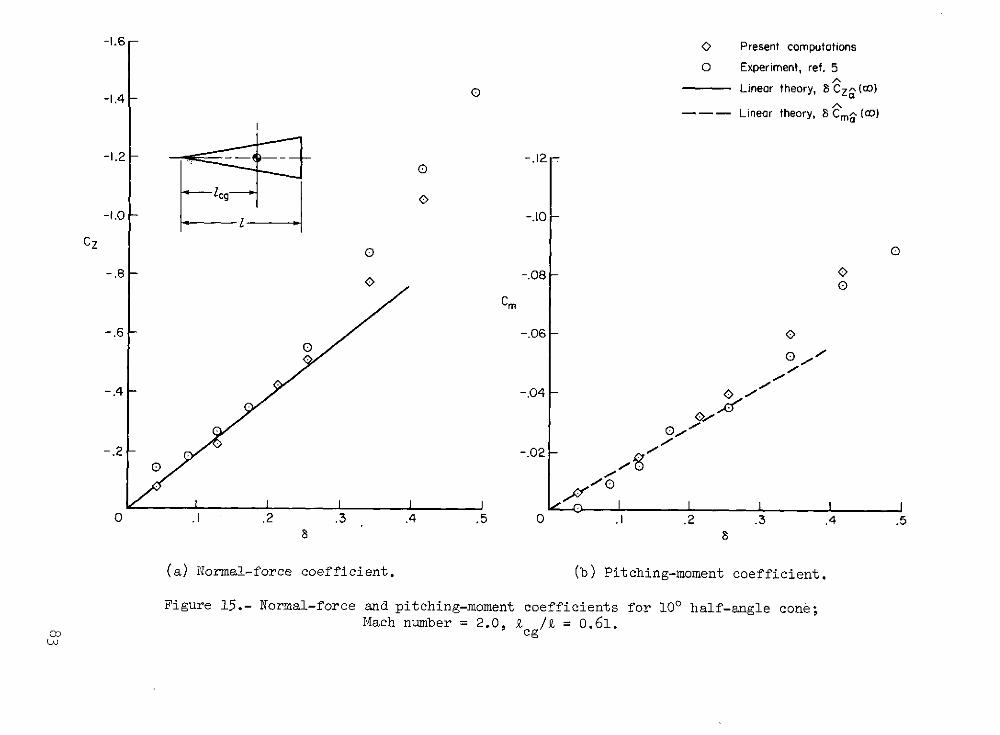
-1.6 O Present computations

0 Experiment, ref. 5

-1.4 Linear theory, 8 CZ (0o)

--- Linear theory, 8 Cm^ (0o)

-1.2 -. 12

OIcg

-1.0 1 -.10O

CZ O 0

-.8 <-.08 -

Cm

- .6 -. 06 <

-. 4 -.04 -

-. 2 0 -. 02 -

0 .1 .2 .3 .4 .5 0 .1 .2 .3 .4 .58 8

(a) Normal-force coefficient. (b) Pitching-moment coefficient.

Figure 15.- Normal-force and pitching-moment coefficients for 100 half-angle cone;Mach number = 2.0, kcg / = 0.61.

0cg

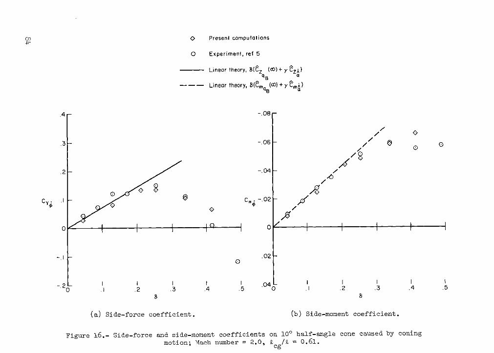
SO Present computations

0 Experiment, ref 5

Linear theory, (Z (co)+ 7y ZA)qB a

--- Linear theory, 8(m (4()+ Ca)

.4- -. 08-

.3- -. 06 -/

/.2- -. 04-

-.I - .02

I I I I I .04 I I I I0 .2 .3 .4 .5 0 . .2 .3 .4 .5

(a) Side-force coefficient. (b) Side-moment coefficient.

Figure 16.- Side-force and side-moment coefficients on 100 half-angle cone caused by coningmotion; Mach number = 2.0, acg / = 0.61.

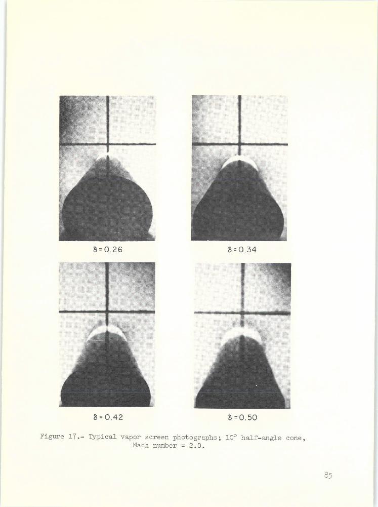
8= 0.26 = 0.34

8= 0.42 8 =0.50

Figure 17.- Typical vapor screen photographs; 100 half-angle cone,Mach number = 2.0.

85

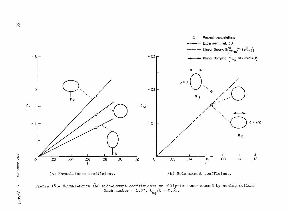
0D

O Present computations

- Experiment, ref. 30

Linear theory, 8( CmqB (O)+yCm )

-.3 --. 03 -. .03 Planar damping (Cn assumed =0)

-. 2 - -. 02 - 2

0 .02 .04 .06 .08 .10 .12 0 .02 .04 .06 .08 .10 .12

Mach number =1.97, cg/A = 0.61.

- /