Embed Size (px)
Citation preview
A STUDY OF TIES AND TIME-VARYING COVARIATES
IN COX PROPORTIONAL HAZARDS MODEL
A Thesis
Presented to
The Faculty of Graduate Studies
of
The University of Guelph
by
XIN XIN
In partial fulfilment of requirements
for the degree of
Master of Science
August, 2011
c© Xin Xin, 2011
ABSTRACT
A STUDY OF TIES AND TIME-VARYING COVARIATES
IN COX PROPORTIONAL HAZARDS MODEL
Xin Xin Advisors:University of Guelph, 2011 Dr. Gerarda Darlington
Dr. Julie Horrocks
In this thesis, ties and time-varying covariates in survival analysis are inves-
tigated. There are two types of ties: ties between event times (Type 1 ties) and ties
between event times and the time that discrete time-varying covariates change or “jump”
(Type 2 ties). The Cox proportional hazards model is one of the most important regres-
sion models for survival analysis. Methods for including Type 1 ties and time-varying
covariates in the Cox proportional hazards model are well established in previous studies,
but Type 2 ties have been ignored in the literature. This thesis discusses the effect of
Type 2 ties on Cox’s partial likelihood, the current default method to treat Type 2 ties
in statistical packages SAS and R (called Fail before Jump in this thesis), and proposes
alternative methods (Random and Equally Weighted) for Type 2 ties. A simulation study
as well as an analysis of data sets from real research both suggest that both Random and
Equally Weighted methods perform better than the other two methods. Also the effect
of the percentages of Type 1 and Type 2 ties on these methods for handling both types
of ties is discussed.
i
Table of Contents
List of Tables ii
List of Figures iii
1 Introduction 1
2 Background 42.1 Cox Proportional Hazards Model . . . . . . . . . . . . . . . . . . . . . . 42.2 Tied Event Times . . . . . . . . . . . . . . . . . . . . . . . . . . . . . . . 4
2.2.1 Exact Method . . . . . . . . . . . . . . . . . . . . . . . . . . . . . 62.2.2 Breslow Approximation . . . . . . . . . . . . . . . . . . . . . . . . 72.2.3 Efron Approximation . . . . . . . . . . . . . . . . . . . . . . . . . 72.2.4 Discrete Method . . . . . . . . . . . . . . . . . . . . . . . . . . . 8
2.3 Cox Proportional Hazards Model with Time-Varying Covariates . . . . . 92.3.1 Time-Varying Covariates in R and SAS . . . . . . . . . . . . . . . 102.3.2 Ties between event Times and Time-dependent Covariates . . . . 13
3 Comparison of Methods for Type 2 Ties 15
4 Simulation of Data Set with Time-Varying Covariates 194.1 Check the Validity of PermAlgo . . . . . . . . . . . . . . . . . . . . . . . 194.2 Simulation of a Population and Analysis of its Samples . . . . . . . . . . 214.3 Percentages of Ties . . . . . . . . . . . . . . . . . . . . . . . . . . . . . . 25
5 Analysis of Real Data Sets 285.1 Stanford Heart Transplant Data Set . . . . . . . . . . . . . . . . . . . . . 295.2 SUD Data Set . . . . . . . . . . . . . . . . . . . . . . . . . . . . . . . . . 31
6 Conclusions and Future Work 34
ii
List of Tables
2.1 Demonstration of Ties between Event Times . . . . . . . . . . . . . . . . 52.2 Original Format of Hypothetical Data Set . . . . . . . . . . . . . . . . . 102.3 Data Format for Counting Process . . . . . . . . . . . . . . . . . . . . . . 122.4 Alternative Data Format for Counting Process . . . . . . . . . . . . . . . 122.5 Demonstration of Ties between Event Times and Jump Times . . . . . . 14
3.1 Three New Data Sets after Ties are Broken . . . . . . . . . . . . . . . . . 163.2 Results of Hypothetical Data Set . . . . . . . . . . . . . . . . . . . . . . 17
4.1 Records for Patients 1 and 2 from the Simulated Data Set . . . . . . . . 204.2 Results of the Four Simulated Populations . . . . . . . . . . . . . . . . . 244.3 Demonstration of Ties Percentages . . . . . . . . . . . . . . . . . . . . . 264.4 Percentages of Events, Jumps and Ties of the Simulated Data Sets . . . . 27
5.1 Heart Transplant Data Set in counting process format . . . . . . . . . . . 305.2 Results of the Heart Transplant Data Set . . . . . . . . . . . . . . . . . 305.3 Statistical Summary of the Full Model for SUD Data Set . . . . . . . . . 325.4 Analysis Results of the SUD Data Set . . . . . . . . . . . . . . . . . . . . 33
6.1 Deviation between Continuous and Default . . . . . . . . . . . . . . . . . 35

iii
List of Figures
4.1 Simulation Procedures . . . . . . . . . . . . . . . . . . . . . . . . . . . . 22
1
Chapter 1
Introduction
If two events are tied, they happen at exactly the same time point. In survival
analysis, ties between event times are important to consider when fitting the Cox pro-
portional hazards models (Cox, 1972) as the Cox partial likelihood depends largely on
the order of events. There are three widely used methods to treat ties between event
times in the Cox proportional hazards model: the exact method (Kalbfleisch and Pren-
tice 2002; DeLong, Guirguis, and So 1994), Breslow approximation (Breslow, 1974) and
Efron approximation (Efron, 1977). Ideally, the exact method should be used as it is the
most accurate but it is also computationally intensive and can be impractical for large
data sets. Both the Breslow approximation and the Efron approximation lead to simpler
and faster calculations. But the Efron approximation is more accurate than the Breslow
approximation, especially when the number of tied event times is large with respect to
the size of the data set (Allison, 2010).
Time-varying covariates are easily accommodated in Cox proportional hazards
model in survival analysis. The values of those covariates change with time, e.g., people’s
age or weight. In many studies, time-varying covariates are the key covariates of interest.
Examples are shown in the following chapters.
In this thesis, only binary time-varying covariates with values 0 and 1 will be
considered. The time at which the binary time-varying covariate changes from 0 to 1 is
called the jump time.
There are two types of ties in most survival data. I will define Type 1 ties as the
2
ties between event times and Type 2 ties as the ties between event times and the time
that time-varying covariates change, i.e., the jump times. All the three methods for tied
event times discussed above were developed for Type 1 ties and have no effect on Type
2 ties. No systematic study has been conducted for Type 2 ties. The objective of this
thesis is to compare methods for treating Type 2 ties in the Cox proportional hazards
model. A simulation study is conducted in R (R Development Core Team, 2011) using the
PermAlgo (Abrahamowicz, Evans, MacKenzie and Sylvestre, 2010) package to simulate
data with time-varying covariates. In addition two real data sets will be analyzed.
One strategy to deal with Type 2 ties is to break the ties. The Type 2 ties can
be manually broken by adding a small positive or negative quantity to the jump times.
Three methods for handling the Type 2 ties can be considered depending on how the small
quantity is added: Fail before Jump, Fail after Jump and Random. Fail before Jump
means a small positive quantity is added to jump times so that the tied event times will
occur before the jump times. Fail after Jump means a small negative quantity is added
to jump times. Random means the small quantity added to the jump time is randomly
positive or negative. Then a Cox proportional hazards model is fitted to obtain regression
coefficient estimates and standard errors corresponding to each of the three methods. A
fourth method, Equally Weighted, is obtained by averaging the regression coefficients of
Fail before Jump and Fail after Jump methods. Standard errors for this method are
proposed, based on the idea of multiple imputation. This thesis will first look at the
default method used in the SAS (SAS Institute Inc., 2010) and R (R Development Core
Team, 2011) to treat Type 2 ties, then will explore alternative methods described above.
To compare the methods for handling the Type 2 ties, 4 populations will be
simulated using the PermAlgo package (Abrahamowicz, Evans, MacKenzie and Sylvestre,
2010) in R (R Development Core Team, 2011). Also two real data sets from clinical
research will be analyzed: the Standford Heart Transplant data set (Crowley & Hu, 1977)
3
and a data set on substance use disorder (SUD) among people who have one parent with
a diagnosis of mood disorder (Duffy, submitted).
It is well known that the Efron approximation and the Breslow approximation
for handling tied event times deteriorate when the amount of ties is large (Allison, 2010;
Hertz-Picciotto and Rockhill, 1997). The performance of methods for the Type 2 ties
presumably will also be affected by the percentages of ties. Strategies to calculate the
percentages of ties will be discussed in this thesis. Also the effect of these percentages on
methods for handling the Type 2 ties will be considered when interpreting results.
4
Chapter 2
Background
2.1 Cox Proportional Hazards Model
Cox (1972) proposed a proportional hazards model for event times when the
event times are continuously distributed and the possibility of ties is ignored. Let zj =
(z1j, ..., zpj) be the values of covariates for the jth individual. Then the hazard function
for time t takes the form:
h(t|zj) = h0(t) exp(zjβ)
where h0(t) is the baseline hazard when zj = 0 and β is a p × 1 vector of regression
coefficients. Cox’s partial likelihood function is used to compute the estimates of the
coefficients, where the partial likelihood is given by:
L(β) =k∏i=1
Li =k∏i=1
exp(ziβ)∑j∈Ri exp(zjβ)
where k is the number of distinct observed event times, zi is the covariate vector at time ti
for the individual who has the event at ti and Ri is the risk set which includes individuals
whose observed event or censoring time is greater than or equal to ti (Lawless, 2003).
2.2 Tied Event Times
In survival analysis, it is quite common for the data sets to contain ties, where
a tie means that two or more individuals in the data set share the same time. Time is
5
usually considered to be a continuous variable, in which case the probability of a tie is
zero. In this thesis, the use of the term continuous will apply to data measured with a
high level of accuracy. In practice, the accuracy of measurement is often more limited and
two observed times can have the same value. For example when the measurement unit
is years, two people that died in the same year will have the same event time recorded,
even though it is very unlikely that they died at the same moment of time.
One assumption of the Cox proportional hazards model is that there are no tied
data. However, in real applications, tied event times are commonly observed and Cox’s
partial likelihood function needs to be modified to handle ties. The following hypothetical
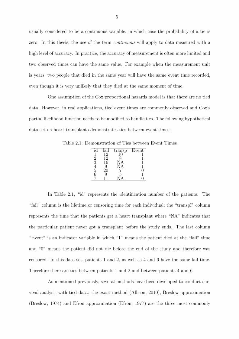
data set on heart transplants demonstrates ties between event times:
Table 2.1: Demonstration of Ties between Event Times
id fail transp Event1 12 10 12 12 8 13 16 NA 14 9 NA 15 20 7 06 9 5 17 11 NA 0
In Table 2.1, “id” represents the identification number of the patients. The
“fail” column is the lifetime or censoring time for each individual; the “transpl” column
represents the time that the patients get a heart transplant where “NA” indicates that
the particular patient never got a transplant before the study ends. The last column
“Event” is an indicator variable in which “1” means the patient died at the “fail” time
and “0” means the patient did not die before the end of the study and therefore was
censored. In this data set, patients 1 and 2, as well as 4 and 6 have the same fail time.
Therefore there are ties between patients 1 and 2 and between patients 4 and 6.
As mentioned previously, several methods have been developed to conduct sur-
vival analysis with tied data: the exact method (Allison, 2010), Breslow approximation
(Breslow, 1974) and Efron approximation (Efron, 1977) are the three most commonly
6
used. The statistical software R (R Development Core Team, 2011) has all the three
methods integrated; SAS (SAS Institute Inc., 2010) also includes all of them but with an
extra method called Discrete (Allison, 2010).
2.2.1 Exact Method
The exact method assumes that the ties arise as a result of imprecise mea-
surement of continuous time, so there exists an underlying ordering for the tied events.
Consequently, when calculating the partial likelihood for the fitted model, all the pos-
sible orderings need to be taken into consideration (Allison, 2010). In the hypothetical
data set, as previously stated, there exists a tie between patient 1 and patient 2. The
exact method assumes that because of the limit of fineness of the measurement, patient
1’s event time can either be before or after patient 2’s event time, which gives us two
possibilities. The partial likelihood will include both possibilities and therefore includes
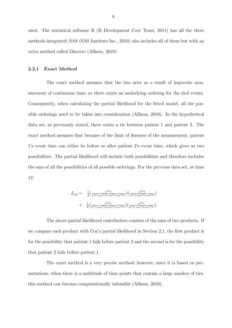
the sum of all the possibilities of all possible orderings. For the previous data set, at time
12:
L12 = 12( eβz1
eβz1+eβz2+eβz3+eβz5)( eβz2
eβz2+eβz3+eβz5)
+ 12( eβz2
eβz1+eβz2+eβz3+eβz5)( eβz1
eβz1+eβz3+eβz5).
The above partial likelihood contribution consists of the sum of two products. If
we compare each product with Cox’s partial likelihood in Section 2.1, the first product is
for the possibility that patient 1 fails before patient 2 and the second is for the possibility
that patient 2 fails before patient 1.
The exact method is a very precise method; however, since it is based on per-
mutations, when there is a multitude of time points that contain a large number of ties,
this method can become computationally infeasible (Allison, 2010).
7
2.2.2 Breslow Approximation
The Breslow approximation assumes that event times are continuous and the
hazard of event is constant in the interval (ti, ti+1) (Breslow, 1974). Also an individual
whose censoring time falls in the interval (ti, ti+1) is assumed to have been censored at
the start of the interval, namely at time ti.
Let zj be the vector of covariate values for the jth individual. Let the set Di
consist of di individuals who failed at the time ti. Let Ri be the risk set at time ti, so Ri
contains all the individuals that are alive or “at risk” at time ti. The partial likelihood
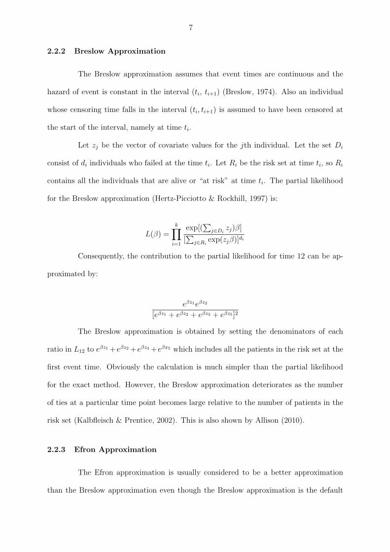
for the Breslow approximation (Hertz-Picciotto & Rockhill, 1997) is:
L(β) =k∏i=1
exp[(∑
j∈Di zj)β]
[∑
j∈Ri exp(zjβ)]di
Consequently, the contribution to the partial likelihood for time 12 can be ap-
proximated by:
eβz1eβz2
[eβz1 + eβz2 + eβz3 + eβz5 ]2
The Breslow approximation is obtained by setting the denominators of each
ratio in L12 to eβz1 +eβz2 +eβz3 +eβx5 which includes all the patients in the risk set at the
first event time. Obviously the calculation is much simpler than the partial likelihood
for the exact method. However, the Breslow approximation deteriorates as the number
of ties at a particular time point becomes large relative to the number of patients in the
risk set (Kalbfleisch & Prentice, 2002). This is also shown by Allison (2010).
2.2.3 Efron Approximation
The Efron approximation is usually considered to be a better approximation
than the Breslow approximation even though the Breslow approximation is the default
8
setting for both SAS (SAS Institute Inc., 2010) and R (R Development Core Team, 2011)
(Allison, 2010). As the percentage of ties increases, the performance of all approximations
becomes worse since their partial likelihoods will become more different from the exact
partial likelihood. The Efron approximation is the same but it is still more accurate than
the other approximations (Allison, 2010; Kalbfleisch & Prentice, 2002).
The partial likelihood function for the Efron’s approximation (Hertz-Picciotto
and Rockhill, 1997) is:
L(β) =k∏i=1
exp[(∑
j∈Di zj)β]∏dil=1[
∑j∈Ri exp(zjβ)− l−1
di
∑j∈Di exp(zjβ)]
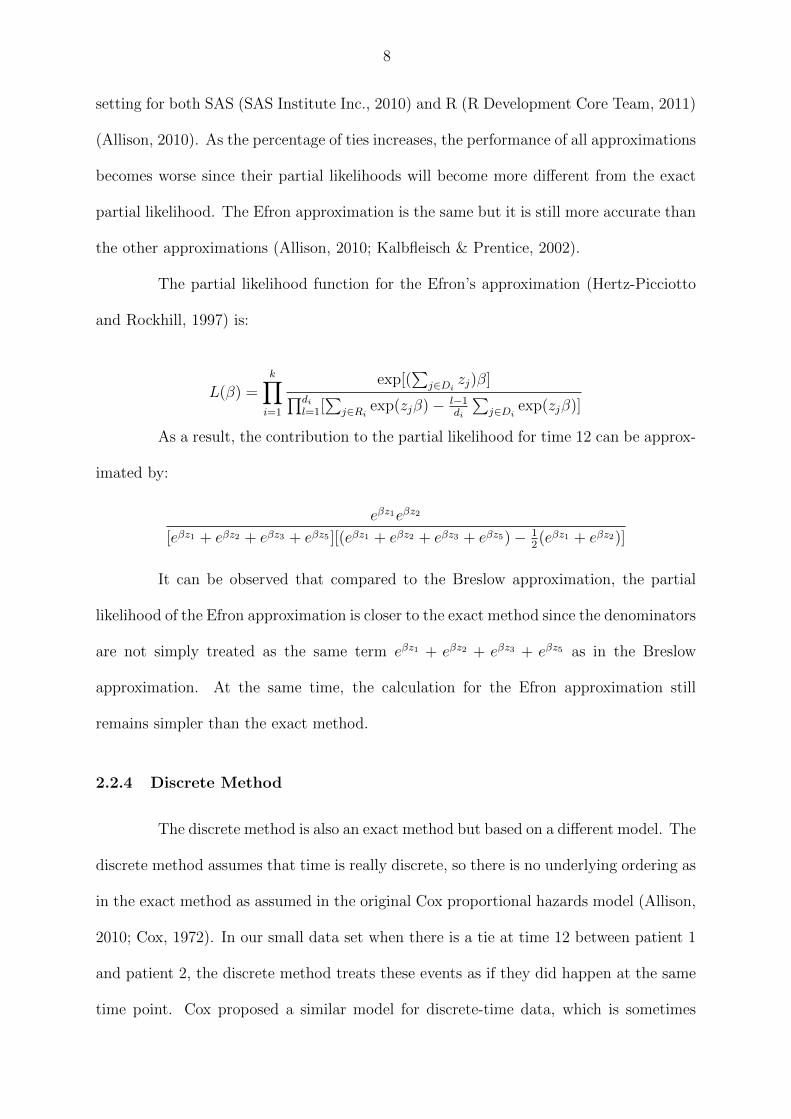
As a result, the contribution to the partial likelihood for time 12 can be approx-
imated by:
eβz1eβz2
[eβz1 + eβz2 + eβz3 + eβz5 ][(eβz1 + eβz2 + eβz3 + eβz5)− 12(eβz1 + eβz2)]
It can be observed that compared to the Breslow approximation, the partial
likelihood of the Efron approximation is closer to the exact method since the denominators
are not simply treated as the same term eβz1 + eβz2 + eβz3 + eβz5 as in the Breslow
approximation. At the same time, the calculation for the Efron approximation still
remains simpler than the exact method.
2.2.4 Discrete Method
The discrete method is also an exact method but based on a different model. The
discrete method assumes that time is really discrete, so there is no underlying ordering as
in the exact method as assumed in the original Cox proportional hazards model (Allison,
2010; Cox, 1972). In our small data set when there is a tie at time 12 between patient 1
and patient 2, the discrete method treats these events as if they did happen at the same
time point. Cox proposed a similar model for discrete-time data, which is sometimes
9
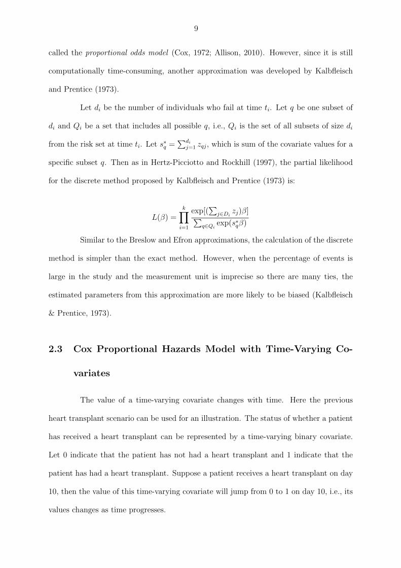
called the proportional odds model (Cox, 1972; Allison, 2010). However, since it is still
computationally time-consuming, another approximation was developed by Kalbfleisch
and Prentice (1973).
Let di be the number of individuals who fail at time ti. Let q be one subset of
di and Qi be a set that includes all possible q, i.e., Qi is the set of all subsets of size di
from the risk set at time ti. Let s∗q =∑di
j=1 zqj, which is sum of the covariate values for a
specific subset q. Then as in Hertz-Picciotto and Rockhill (1997), the partial likelihood
for the discrete method proposed by Kalbfleisch and Prentice (1973) is:
L(β) =k∏i=1
exp[(∑
j∈Di zj)β]∑q∈Qi exp(s∗qβ)
Similar to the Breslow and Efron approximations, the calculation of the discrete
method is simpler than the exact method. However, when the percentage of events is
large in the study and the measurement unit is imprecise so there are many ties, the
estimated parameters from this approximation are more likely to be biased (Kalbfleisch
& Prentice, 1973).
2.3 Cox Proportional Hazards Model with Time-Varying Co-
variates
The value of a time-varying covariate changes with time. Here the previous
heart transplant scenario can be used for an illustration. The status of whether a patient
has received a heart transplant can be represented by a time-varying binary covariate.
Let 0 indicate that the patient has not had a heart transplant and 1 indicate that the
patient has had a heart transplant. Suppose a patient receives a heart transplant on day
10, then the value of this time-varying covariate will jump from 0 to 1 on day 10, i.e., its
values changes as time progresses.
10
I will only discuss binary time-varying covariates with values 0 and 1 in my
thesis. The time at which the value of the time-varying covariates changes is referred to
the jump time.
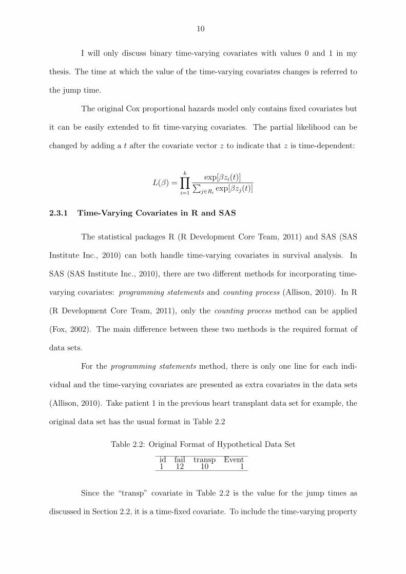
The original Cox proportional hazards model only contains fixed covariates but
it can be easily extended to fit time-varying covariates. The partial likelihood can be
changed by adding a t after the covariate vector z to indicate that z is time-dependent:
L(β) =k∏i=1
exp[βzi(t)]∑j∈Ri exp[βzj(t)]
2.3.1 Time-Varying Covariates in R and SAS
The statistical packages R (R Development Core Team, 2011) and SAS (SAS
Institute Inc., 2010) can both handle time-varying covariates in survival analysis. In
SAS (SAS Institute Inc., 2010), there are two different methods for incorporating time-
varying covariates: programming statements and counting process (Allison, 2010). In R
(R Development Core Team, 2011), only the counting process method can be applied
(Fox, 2002). The main difference between these two methods is the required format of
data sets.
For the programming statements method, there is only one line for each indi-
vidual and the time-varying covariates are presented as extra covariates in the data sets
(Allison, 2010). Take patient 1 in the previous heart transplant data set for example, the
original data set has the usual format in Table 2.2
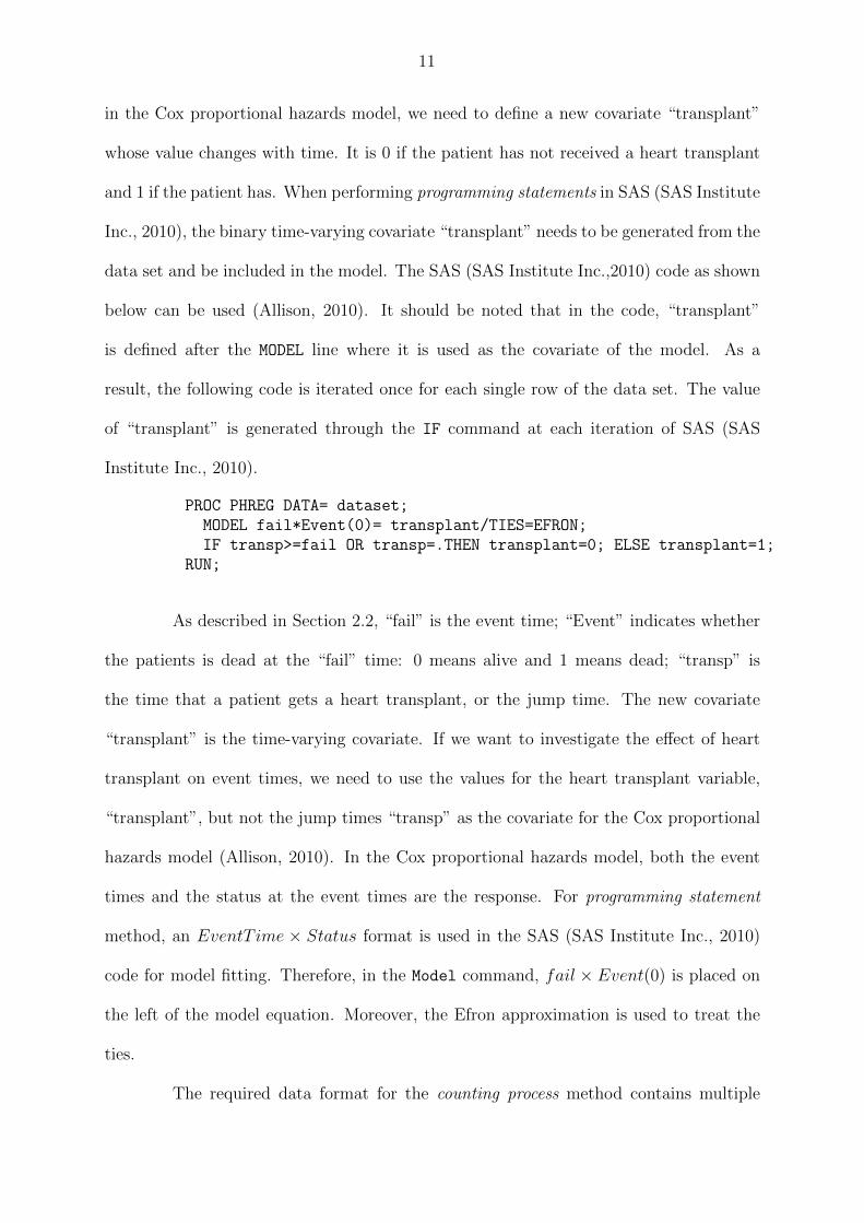
Table 2.2: Original Format of Hypothetical Data Set
id fail transp Event1 12 10 1
Since the “transp” covariate in Table 2.2 is the value for the jump times as
discussed in Section 2.2, it is a time-fixed covariate. To include the time-varying property
11
in the Cox proportional hazards model, we need to define a new covariate “transplant”
whose value changes with time. It is 0 if the patient has not received a heart transplant
and 1 if the patient has. When performing programming statements in SAS (SAS Institute
Inc., 2010), the binary time-varying covariate “transplant” needs to be generated from the
data set and be included in the model. The SAS (SAS Institute Inc.,2010) code as shown
below can be used (Allison, 2010). It should be noted that in the code, “transplant”
is defined after the MODEL line where it is used as the covariate of the model. As a
result, the following code is iterated once for each single row of the data set. The value
of “transplant” is generated through the IF command at each iteration of SAS (SAS
Institute Inc., 2010).
PROC PHREG DATA= dataset;MODEL fail*Event(0)= transplant/TIES=EFRON;IF transp>=fail OR transp=.THEN transplant=0; ELSE transplant=1;
RUN;
As described in Section 2.2, “fail” is the event time; “Event” indicates whether
the patients is dead at the “fail” time: 0 means alive and 1 means dead; “transp” is
the time that a patient gets a heart transplant, or the jump time. The new covariate
“transplant” is the time-varying covariate. If we want to investigate the effect of heart
transplant on event times, we need to use the values for the heart transplant variable,
“transplant”, but not the jump times “transp” as the covariate for the Cox proportional
hazards model (Allison, 2010). In the Cox proportional hazards model, both the event
times and the status at the event times are the response. For programming statement
method, an EventT ime × Status format is used in the SAS (SAS Institute Inc., 2010)
code for model fitting. Therefore, in the Model command, fail × Event(0) is placed on
the left of the model equation. Moreover, the Efron approximation is used to treat the
ties.
The required data format for the counting process method contains multiple
12
lines for each individual. Each line represents a time interval in which the time-varying
covariates stay constant or a time interval that represents one unit increase of time, e.g,
one year (Allison, 2010; Fox, 2002).
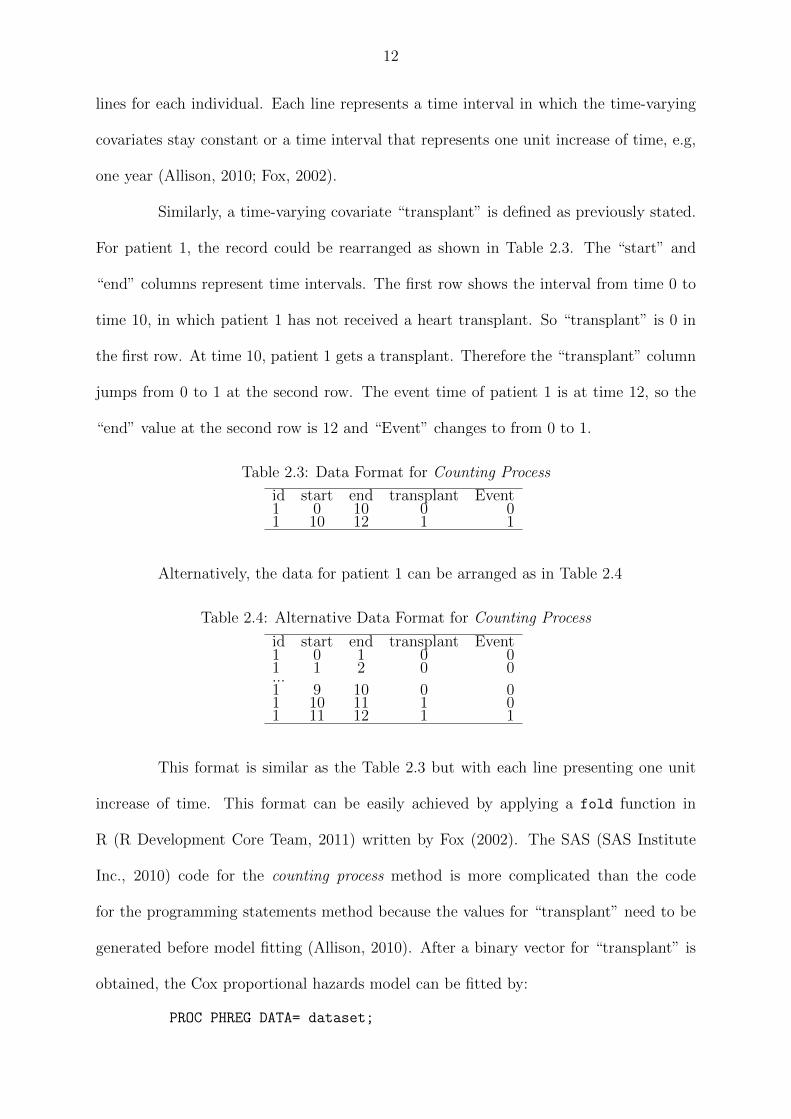
Similarly, a time-varying covariate “transplant” is defined as previously stated.
For patient 1, the record could be rearranged as shown in Table 2.3. The “start” and
“end” columns represent time intervals. The first row shows the interval from time 0 to
time 10, in which patient 1 has not received a heart transplant. So “transplant” is 0 in
the first row. At time 10, patient 1 gets a transplant. Therefore the “transplant” column
jumps from 0 to 1 at the second row. The event time of patient 1 is at time 12, so the
“end” value at the second row is 12 and “Event” changes to from 0 to 1.
Table 2.3: Data Format for Counting Process
id start end transplant Event1 0 10 0 01 10 12 1 1
Alternatively, the data for patient 1 can be arranged as in Table 2.4
Table 2.4: Alternative Data Format for Counting Process
id start end transplant Event1 0 1 0 01 1 2 0 0...1 9 10 0 01 10 11 1 01 11 12 1 1
This format is similar as the Table 2.3 but with each line presenting one unit
increase of time. This format can be easily achieved by applying a fold function in
R (R Development Core Team, 2011) written by Fox (2002). The SAS (SAS Institute
Inc., 2010) code for the counting process method is more complicated than the code
for the programming statements method because the values for “transplant” need to be
generated before model fitting (Allison, 2010). After a binary vector for “transplant” is
obtained, the Cox proportional hazards model can be fitted by:
PROC PHREG DATA= dataset;
13
MODEL (start, end)*Event(0)= transplant/TIES=EFRON;RUN;
Instead of using the usual (event Time * status) format for the left side of
the model, a (start, stop)*status format is used (Allison, 2010).
R (R Development Core Team, 2011) cannot perform the programming state-
ments methods. For counting process, the R (R Development Core Team, 2011) code is
very similar to the SAS (SAS Institute Inc., 2010) code:
model <- coxph(Surv(Start, Stop, Event)~ transplant, method="efron", data)
The R package Surival (Therneau & Lumley, 2011) needs to be loaded. The
coxph command is for model fitting and the Surv command is for constructing a survival
object as the response of the Cox proportional hazards model. The detailed coding for R
(R Development Core Team, 2011) and SAS (SAS Institute Inc., 2010) with time-varying
covariates will be illustrated in following chapters.
2.3.2 Ties between event Times and Time-dependent Covariates
As previously defined, there are mainly two different types of ties in life time
data. The Type 1 ties are the ties between event times as discussed in the last section,
i.e., different individuals with the same event time. The Type 2 ties are the ties between
event times and the times that discrete time-varying covariates change among different
individuals (the jump time). The Type 2 ties have been ignored in the literature.
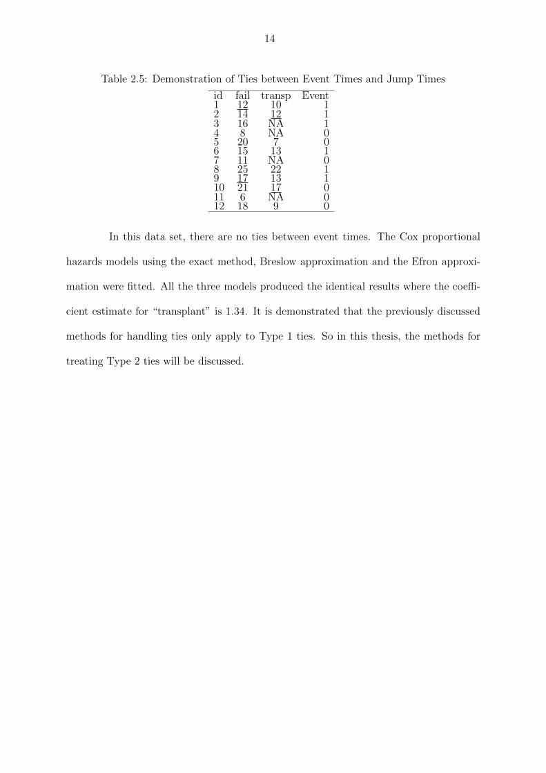
Table 2.5 is a similar data set as in Table 2.1 created as an illustration for the
Type 2 ties. There are 12 patients in the data set. The event time of patient 1 is 12
and the transplant time for patient 2 is 12. So there is a tie between the event time of
patient 1 and the jump time of patient 2. Similarly, the event time of patient 9 and the
jump time of patient 10 are tied. Note that patient 2 is observed to fail while patient 10
is censored.
14
Table 2.5: Demonstration of Ties between Event Times and Jump Times
id fail transp Event1 12 10 12 14 12 13 16 NA 14 8 NA 05 20 7 06 15 13 17 11 NA 08 25 22 19 17 13 110 21 17 011 6 NA 012 18 9 0
In this data set, there are no ties between event times. The Cox proportional
hazards models using the exact method, Breslow approximation and the Efron approxi-
mation were fitted. All the three models produced the identical results where the coeffi-
cient estimate for “transplant” is 1.34. It is demonstrated that the previously discussed
methods for handling ties only apply to Type 1 ties. So in this thesis, the methods for
treating Type 2 ties will be discussed.
15
Chapter 3
Comparison of Methods for Type 2 Ties
To investigate how SAS (SAS Institute Inc., 2010) and R (R Development Core
Team, 2011) implement the Cox proportional hazards model with Type 2 ties, I will
change certain values of the hypothetical heart transplant data set discussed in Section
2.2 so that the ties are forced to be broken. Then the results of the original and altered
data sets will be compared. The two packages are expected to produce the same results.
Also these packages automatically treat the time-varying covariates as if they changed
after the (tied) event time, although the user can control this by subtracting a small
amount from the covariate change time. This will be verified in the following analysis.
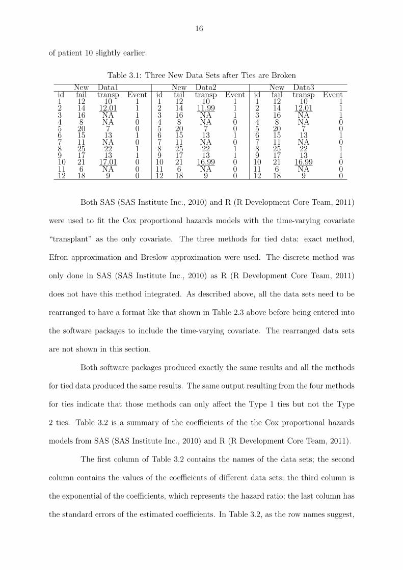
In the data set in Table 2.5 there are two Type 2 ties. One is between the event
time of patient 1 and the jump time of patient 2; the other one is between the event time
of patient 9 and the jump time of patient 10. Three new data sets can be obtained if the
two ties are forced to be broken: Fail before Jump, Fail after Jump and Random. They
are shown as under New Data1, New Data2 and New Data3, respectively, in Table 3.1.
For Fail before Jump, a small amount of time is added to the jump times of
patient 2 and patient 10, so that the event times occur before the jump times. For Fail
after Jump, under New Data2 in the middle of the table, the jump times are adjusted
by subtracting a small amount, so that event times occur slightly after the (tied) jump
times. For Random shown under New Data3, the jump times are each randomly adjusted
to be before or after the event times. However, due to the simplicity of this data set, this
is done by manually shifting the jump time of patient 2 slightly later and the jump time
16
of patient 10 slightly earlier.
Table 3.1: Three New Data Sets after Ties are Broken
New Data1 New Data2 New Data3id fail transp Event id fail transp Event id fail transp Event1 12 10 1 1 12 10 1 1 12 10 12 14 12.01 1 2 14 11.99 1 2 14 12.01 13 16 NA 1 3 16 NA 1 3 16 NA 14 8 NA 0 4 8 NA 0 4 8 NA 05 20 7 0 5 20 7 0 5 20 7 06 15 13 1 6 15 13 1 6 15 13 17 11 NA 0 7 11 NA 0 7 11 NA 08 25 22 1 8 25 22 1 8 25 22 19 17 13 1 9 17 13 1 9 17 13 110 21 17.01 0 10 21 16.99 0 10 21 16.99 011 6 NA 0 11 6 NA 0 11 6 NA 012 18 9 0 12 18 9 0 12 18 9 0
Both SAS (SAS Institute Inc., 2010) and R (R Development Core Team, 2011)
were used to fit the Cox proportional hazards models with the time-varying covariate
“transplant” as the only covariate. The three methods for tied data: exact method,
Efron approximation and Breslow approximation were used. The discrete method was
only done in SAS (SAS Institute Inc., 2010) as R (R Development Core Team, 2011)
does not have this method integrated. As described above, all the data sets need to be
rearranged to have a format like that shown in Table 2.3 above before being entered into
the software packages to include the time-varying covariate. The rearranged data sets
are not shown in this section.
Both software packages produced exactly the same results and all the methods
for tied data produced the same results. The same output resulting from the four methods
for ties indicate that those methods can only affect the Type 1 ties but not the Type
2 ties. Table 3.2 is a summary of the coefficients of the the Cox proportional hazards
models from SAS (SAS Institute Inc., 2010) and R (R Development Core Team, 2011).
The first column of Table 3.2 contains the names of the data sets; the second
column contains the values of the coefficients of different data sets; the third column is
the exponential of the coefficients, which represents the hazard ratio; the last column has
the standard errors of the estimated coefficients. In Table 3.2, as the row names suggest,
17
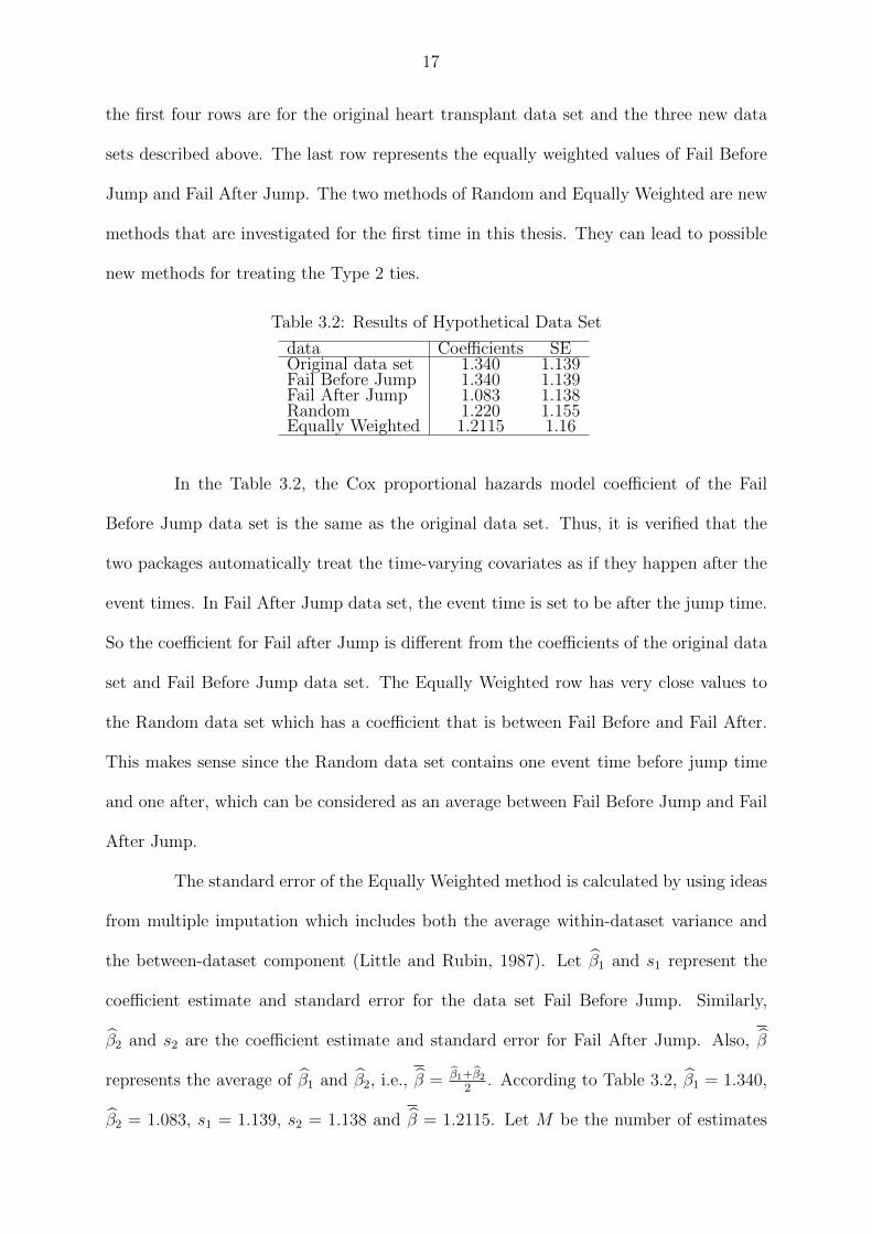
the first four rows are for the original heart transplant data set and the three new data
sets described above. The last row represents the equally weighted values of Fail Before
Jump and Fail After Jump. The two methods of Random and Equally Weighted are new
methods that are investigated for the first time in this thesis. They can lead to possible
new methods for treating the Type 2 ties.
Table 3.2: Results of Hypothetical Data Set
data Coefficients SEOriginal data set 1.340 1.139Fail Before Jump 1.340 1.139Fail After Jump 1.083 1.138Random 1.220 1.155Equally Weighted 1.2115 1.16
In the Table 3.2, the Cox proportional hazards model coefficient of the Fail
Before Jump data set is the same as the original data set. Thus, it is verified that the
two packages automatically treat the time-varying covariates as if they happen after the
event times. In Fail After Jump data set, the event time is set to be after the jump time.
So the coefficient for Fail after Jump is different from the coefficients of the original data
set and Fail Before Jump data set. The Equally Weighted row has very close values to
the Random data set which has a coefficient that is between Fail Before and Fail After.
This makes sense since the Random data set contains one event time before jump time
and one after, which can be considered as an average between Fail Before Jump and Fail
After Jump.
The standard error of the Equally Weighted method is calculated by using ideas
from multiple imputation which includes both the average within-dataset variance and
the between-dataset component (Little and Rubin, 1987). Let β̂1 and s1 represent the
coefficient estimate and standard error for the data set Fail Before Jump. Similarly,
β̂2 and s2 are the coefficient estimate and standard error for Fail After Jump. Also, β̂
represents the average of β̂1 and β̂2, i.e., β̂ = β̂1+β̂22
. According to Table 3.2, β̂1 = 1.340,
β̂2 = 1.083, s1 = 1.139, s2 = 1.138 and β̂ = 1.2115. Let M be the number of estimates
18
being combined. The Equally Weighted coefficient is the average of Fail Before Jump
and Fail After Jump, which suggests that M = 2.
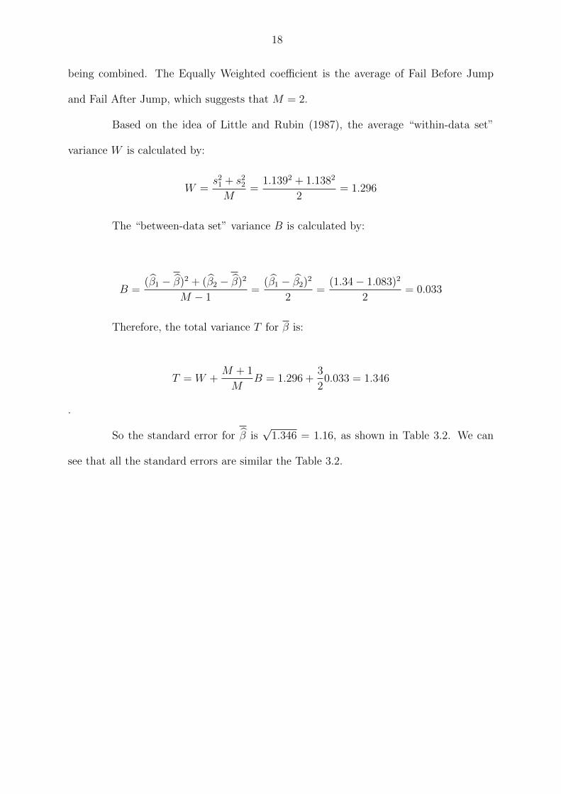
Based on the idea of Little and Rubin (1987), the average “within-data set”
variance W is calculated by:
W =s21 + s22M
=1.1392 + 1.1382
2= 1.296
The “between-data set” variance B is calculated by:
B =(β̂1 − β̂)2 + (β̂2 − β̂)2
M − 1=
(β̂1 − β̂2)2
2=
(1.34− 1.083)2
2= 0.033
Therefore, the total variance T for β is:
T = W +M + 1
MB = 1.296 +
3
20.033 = 1.346
.
So the standard error for β̂ is√
1.346 = 1.16, as shown in Table 3.2. We can
see that all the standard errors are similar the Table 3.2.
19
Chapter 4
Simulation of Data Set with Time-Varying
Covariates
The simulation of survival data with time-varying covariates can be carried out
by using the “PermAlgo” package (Abrahamowicz, Evans, MacKenzie and Sylvestre,
2010) in R (R Development Core Team, 2011). The package requires the number of
individuals (n), the maximum follow up time for the individuals (m), a matrix containing
the covariate values (Xmat), the regression coefficient vector (beta), the event time and
censoring time for each individual. The ordering of the event times and censoring times
are assumed to be completely random, i.e., not in the same order as the covariates. The
program will assign covariate values to event/censoring times in such a way that the data
conforms to the Cox proportional hazards model with regression coefficient vector beta
and x variables as in Xmat (Abrahamowicz, Evans, MacKenzie and Sylvestre, 2010).
4.1 Check the Validity of PermAlgo
I generated a data set under the heart transplant scenario. It contains 100
individuals. The event (death) time for each individual is randomly selected from an
exponential distribution with parameter λ = 0.05. The censoring time is randomly
selected from a uniform distribution with range (1, 20) so that there is variety of failure
and censoring. The maximum length of follow-up time is set to be 20, which means that
the individuals fail or are censored by time 20. There is one time-varying covariate as
20
the only covariate, representing “transplant”.
The coefficient of this covariate (the log hazard ratio) was originally set to be
log 2 = 0.693. Since there is only one covariate, Xmat is a matrix with one column
and n × m = 2000 rows. Since Xmat represents the binary time-dependent covariate
“transplant”, a jump time needs to be specified for each patient. The jump time is
randomly generated from a uniform distribution with range (1, 20). For each individual,
the value for transplant is 0 before the jump time and 1 after the jump time.
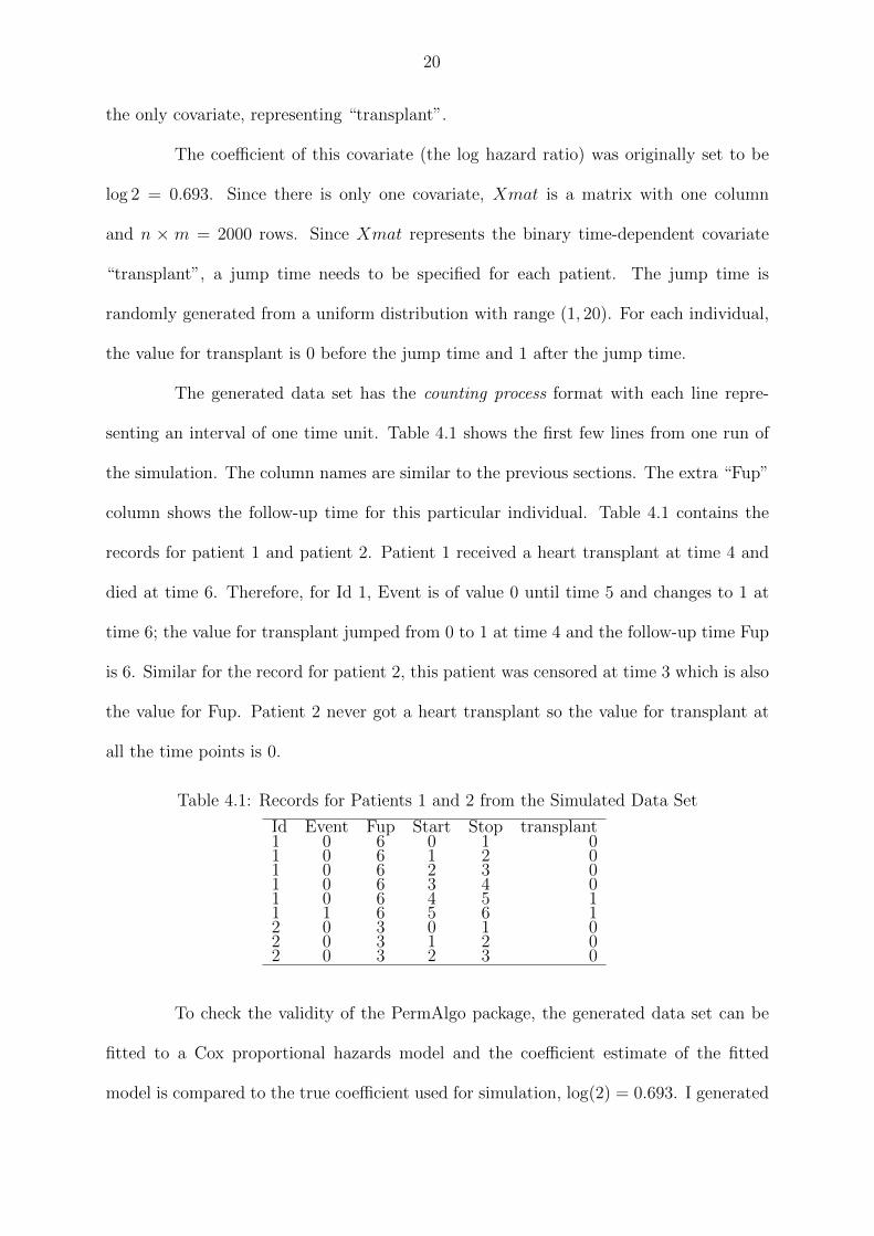
The generated data set has the counting process format with each line repre-
senting an interval of one time unit. Table 4.1 shows the first few lines from one run of
the simulation. The column names are similar to the previous sections. The extra “Fup”
column shows the follow-up time for this particular individual. Table 4.1 contains the
records for patient 1 and patient 2. Patient 1 received a heart transplant at time 4 and
died at time 6. Therefore, for Id 1, Event is of value 0 until time 5 and changes to 1 at
time 6; the value for transplant jumped from 0 to 1 at time 4 and the follow-up time Fup
is 6. Similar for the record for patient 2, this patient was censored at time 3 which is also
the value for Fup. Patient 2 never got a heart transplant so the value for transplant at
all the time points is 0.
Table 4.1: Records for Patients 1 and 2 from the Simulated Data Set
Id Event Fup Start Stop transplant1 0 6 0 1 01 0 6 1 2 01 0 6 2 3 01 0 6 3 4 01 0 6 4 5 11 1 6 5 6 12 0 3 0 1 02 0 3 1 2 02 0 3 2 3 0
To check the validity of the PermAlgo package, the generated data set can be
fitted to a Cox proportional hazards model and the coefficient estimate of the fitted
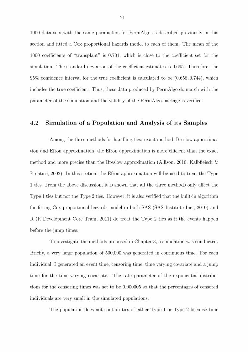
model is compared to the true coefficient used for simulation, log(2) = 0.693. I generated
21
1000 data sets with the same parameters for PermAlgo as described previously in this
section and fitted a Cox proportional hazards model to each of them. The mean of the
1000 coefficients of “transplant” is 0.701, which is close to the coefficient set for the
simulation. The standard deviation of the coefficient estimates is 0.695. Therefore, the
95% confidence interval for the true coefficient is calculated to be (0.658, 0.744), which
includes the true coefficient. Thus, these data produced by PermAlgo do match with the
parameter of the simulation and the validity of the PermAlgo package is verified.
4.2 Simulation of a Population and Analysis of its Samples
Among the three methods for handling ties: exact method, Breslow approxima-
tion and Efron approximation, the Efron approximation is more efficient than the exact
method and more precise than the Breslow approximation (Allison, 2010; Kalbfleisch &
Prentice, 2002). In this section, the Efron approximation will be used to treat the Type
1 ties. From the above discussion, it is shown that all the three methods only affect the
Type 1 ties but not the Type 2 ties. However, it is also verified that the built-in algorithm
for fitting Cox proportional hazards model in both SAS (SAS Institute Inc., 2010) and
R (R Development Core Team, 2011) do treat the Type 2 ties as if the events happen
before the jump times.
To investigate the methods proposed in Chapter 3, a simulation was conducted.
Briefly, a very large population of 500,000 was generated in continuous time. For each
individual, I generated an event time, censoring time, time varying covariate and a jump
time for the time-varying covariate. The rate parameter of the exponential distribu-
tions for the censoring times was set to be 0.000005 so that the percentages of censored
individuals are very small in the simulated populations.
The population does not contain ties of either Type 1 or Type 2 because time
22
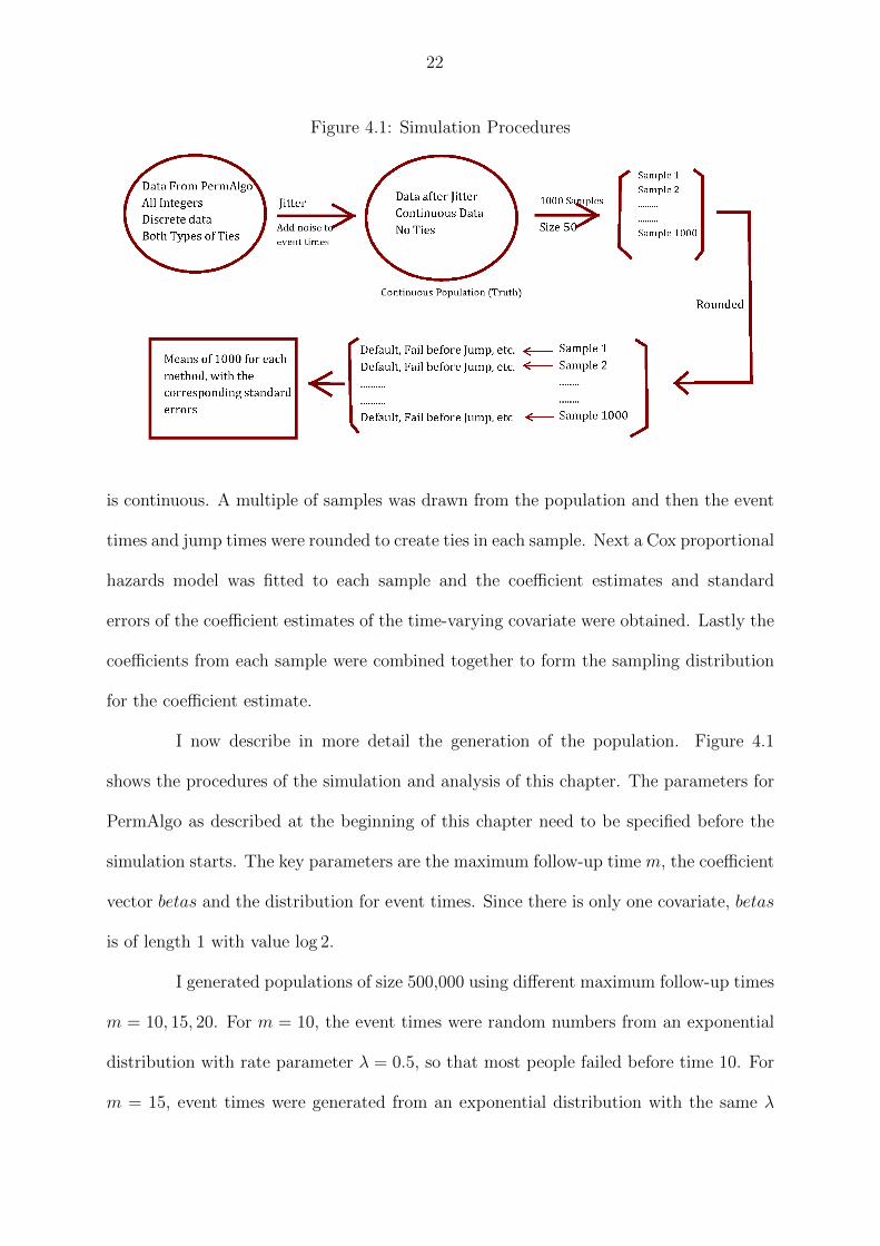
Figure 4.1: Simulation Procedures
is continuous. A multiple of samples was drawn from the population and then the event
times and jump times were rounded to create ties in each sample. Next a Cox proportional
hazards model was fitted to each sample and the coefficient estimates and standard
errors of the coefficient estimates of the time-varying covariate were obtained. Lastly the
coefficients from each sample were combined together to form the sampling distribution
for the coefficient estimate.
I now describe in more detail the generation of the population. Figure 4.1
shows the procedures of the simulation and analysis of this chapter. The parameters for
PermAlgo as described at the beginning of this chapter need to be specified before the
simulation starts. The key parameters are the maximum follow-up time m, the coefficient
vector betas and the distribution for event times. Since there is only one covariate, betas
is of length 1 with value log 2.
I generated populations of size 500,000 using different maximum follow-up times
m = 10, 15, 20. For m = 10, the event times were random numbers from an exponential
distribution with rate parameter λ = 0.5, so that most people failed before time 10. For
m = 15, event times were generated from an exponential distribution with the same λ
23
as for m = 10. But consequently, when λ = 0.5 most people would fail before time
10. So the population with m = 15 would be quite close to the population with m=10.
Therefore, another population for m = 15 with event times produced with λ = 0.25 was
simulated. In this case most people failed before time 15, but there still was a reasonable
number of individuals that failed between time 10 and time 15. For the population with
m = 20, only one population with event time distribution λ = 0.5 was generated. In
summary, there are 4 populations in total each with size 500,000.
Unfortunately, the values of time in data sets generated by PermAlgo are all
integers, which means that there are many ties in the data of both types. They are the
data sets in the first circle in Figure 4.1. To create the populations in which time is a
continuous variable, I added noise to all the event times by using a jitter function in R
(R Development Core Team, 2011).
By setting the amount parameter to be 0.4 in the jitter function, a different
value from a uniform distribution with range [−0.4, 0.4] is added to each of the event
times. Therefore, in the population, there are no tied event times and the orderings of all
event times and jump times are known. These populations are shown in the second circle
in Figure 4.1. The value of β for each population was found by fitting a Cox proportional
hazards model in R (R Development Core Team, 2011) to the whole population. The β
values are shown in Table 4.2.
Finally, from each of the 4 populations, 1000 samples each with sample size 50
are randomly drawn and then event time values are rounded to create ties. In this way,
the true orderings between event and jump times are known in the populations but not
in the samples. These steps are also shown in Figure 4.1.
The data from each sample were analyzed using the methods from Chapter 3.
Specifically, in each sample, 0.01 is added or subtracted from the jump times so that the
ties are manually broken. Then the coefficients and standard errors for the time varying
24
covariates estimated using the methods described in Chapter 3 (default method, Fail
before Jump, Fail after Jump, Random, and Equally Weighted) are obtained by fitting a
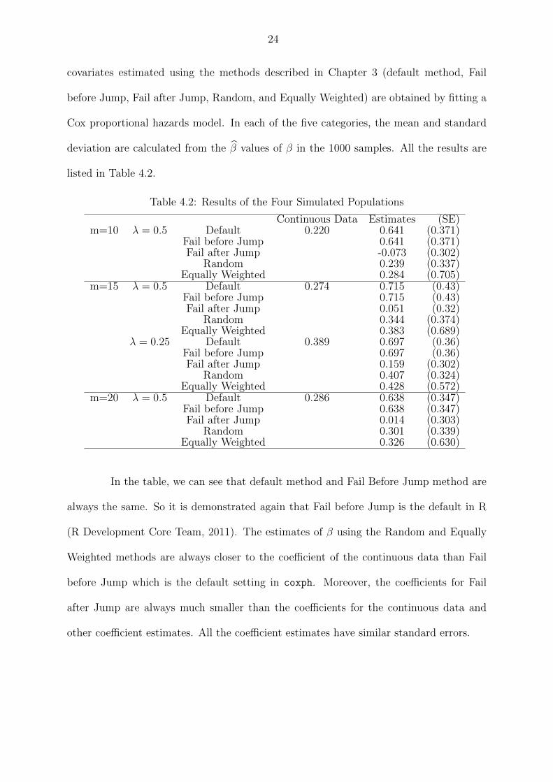
Cox proportional hazards model. In each of the five categories, the mean and standard
deviation are calculated from the β̂ values of β in the 1000 samples. All the results are
listed in Table 4.2.
Table 4.2: Results of the Four Simulated Populations
Continuous Data Estimates (SE)m=10 λ = 0.5 Default 0.220 0.641 (0.371)
Fail before Jump 0.641 (0.371)Fail after Jump -0.073 (0.302)
Random 0.239 (0.337)Equally Weighted 0.284 (0.705)
m=15 λ = 0.5 Default 0.274 0.715 (0.43)Fail before Jump 0.715 (0.43)Fail after Jump 0.051 (0.32)
Random 0.344 (0.374)Equally Weighted 0.383 (0.689)
λ = 0.25 Default 0.389 0.697 (0.36)Fail before Jump 0.697 (0.36)Fail after Jump 0.159 (0.302)
Random 0.407 (0.324)Equally Weighted 0.428 (0.572)
m=20 λ = 0.5 Default 0.286 0.638 (0.347)Fail before Jump 0.638 (0.347)Fail after Jump 0.014 (0.303)
Random 0.301 (0.339)Equally Weighted 0.326 (0.630)
In the table, we can see that default method and Fail Before Jump method are
always the same. So it is demonstrated again that Fail before Jump is the default in R
(R Development Core Team, 2011). The estimates of β using the Random and Equally
Weighted methods are always closer to the coefficient of the continuous data than Fail
before Jump which is the default setting in coxph. Moreover, the coefficients for Fail
after Jump are always much smaller than the coefficients for the continuous data and
other coefficient estimates. All the coefficient estimates have similar standard errors.
25
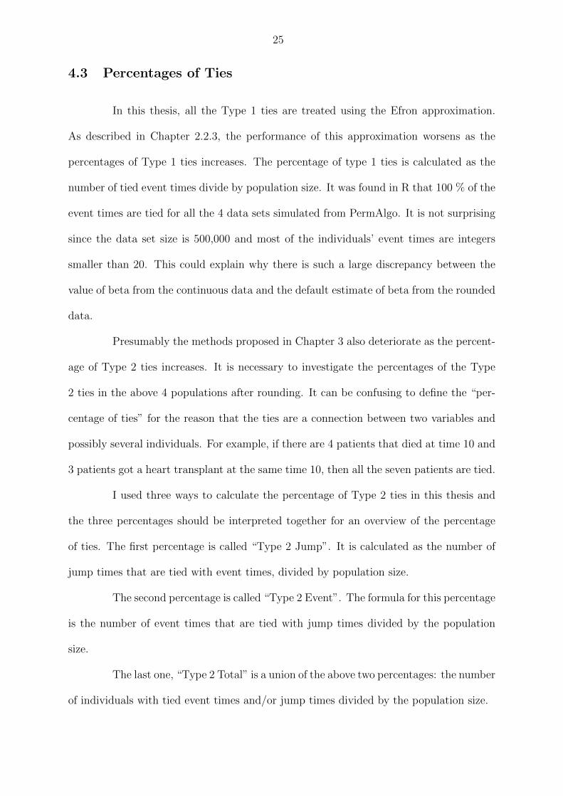
4.3 Percentages of Ties
In this thesis, all the Type 1 ties are treated using the Efron approximation.
As described in Chapter 2.2.3, the performance of this approximation worsens as the
percentages of Type 1 ties increases. The percentage of type 1 ties is calculated as the
number of tied event times divide by population size. It was found in R that 100 % of the
event times are tied for all the 4 data sets simulated from PermAlgo. It is not surprising
since the data set size is 500,000 and most of the individuals’ event times are integers
smaller than 20. This could explain why there is such a large discrepancy between the
value of beta from the continuous data and the default estimate of beta from the rounded
data.
Presumably the methods proposed in Chapter 3 also deteriorate as the percent-
age of Type 2 ties increases. It is necessary to investigate the percentages of the Type
2 ties in the above 4 populations after rounding. It can be confusing to define the “per-
centage of ties” for the reason that the ties are a connection between two variables and
possibly several individuals. For example, if there are 4 patients that died at time 10 and
3 patients got a heart transplant at the same time 10, then all the seven patients are tied.
I used three ways to calculate the percentage of Type 2 ties in this thesis and
the three percentages should be interpreted together for an overview of the percentage
of ties. The first percentage is called “Type 2 Jump”. It is calculated as the number of
jump times that are tied with event times, divided by population size.
The second percentage is called “Type 2 Event”. The formula for this percentage
is the number of event times that are tied with jump times divided by the population
size.
The last one, “Type 2 Total” is a union of the above two percentages: the number
of individuals with tied event times and/or jump times divided by the population size.
26
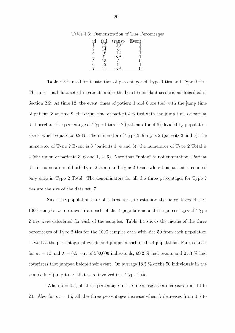
Table 4.3: Demonstration of Ties Percentages
id fail transp Event1 12 10 12 14 8 13 16 12 14 9 NA 15 13 5 06 12 9 17 11 NA 0
Table 4.3 is used for illustration of percentages of Type 1 ties and Type 2 ties.
This is a small data set of 7 patients under the heart transplant scenario as described in
Section 2.2. At time 12, the event times of patient 1 and 6 are tied with the jump time
of patient 3; at time 9, the event time of patient 4 is tied with the jump time of patient
6. Therefore, the percentage of Type 1 ties is 2 (patients 1 and 6) divided by population
size 7, which equals to 0.286. The numerator of Type 2 Jump is 2 (patients 3 and 6); the
numerator of Type 2 Event is 3 (patients 1, 4 and 6); the numerator of Type 2 Total is
4 (the union of patients 3, 6 and 1, 4, 6). Note that “union” is not summation. Patient
6 is in numerators of both Type 2 Jump and Type 2 Event,while this patient is counted
only once in Type 2 Total. The denominators for all the three percentages for Type 2
ties are the size of the data set, 7.
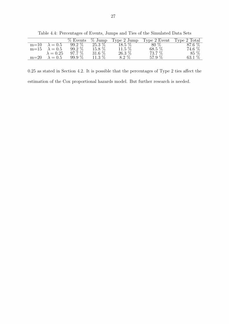
Since the populations are of a large size, to estimate the percentages of ties,
1000 samples were drawn from each of the 4 populations and the percentages of Type
2 ties were calculated for each of the samples. Table 4.4 shows the means of the three
percentages of Type 2 ties for the 1000 samples each with size 50 from each population
as well as the percentages of events and jumps in each of the 4 population. For instance,
for m = 10 and λ = 0.5, out of 500,000 individuals, 99.2 % had events and 25.3 % had
covariates that jumped before their event. On average 18.5 % of the 50 individuals in the
sample had jump times that were involved in a Type 2 tie.
When λ = 0.5, all three percentages of ties decrease as m increases from 10 to
20. Also for m = 15, all the three percentages increase when λ decreases from 0.5 to
27
Table 4.4: Percentages of Events, Jumps and Ties of the Simulated Data Sets
% Events % Jump Type 2 Jump Type 2 Event Type 2 Totalm=10 λ = 0.5 99.2 % 25.3 % 18.5 % 80 % 87.6 %m=15 λ = 0.5 99.2 % 15.8 % 11.5 % 68.5 % 74.6 %
λ = 0.25 97.7 % 31.6 % 26.3 % 73.7 % 85 %m=20 λ = 0.5 99.9 % 11.3 % 8.2 % 57.9 % 63.1 %
0.25 as stated in Section 4.2. It is possible that the percentages of Type 2 ties affect the
estimation of the Cox proportional hazards model. But further research is needed.
28
Chapter 5
Analysis of Real Data Sets
In this section I will provide results from analyzing two data sets from medical
research. For each data set, the analysis will follow similar strategies as the analysis of
the simulated data in Chapter 4.2. In order to investigate ties, an artificial scenario will
be created in which we have access to both a continuous and rounded version of the data.
For both analyses, the continuous data set (in which time is continuous, there are no ties,
and the order of event and jump times is known) will be compared to the rounded data
set (in which time is discrete, there are ties, and the order of event and jump times is
unknown). The continuous data set will then be considered to be the actual data, while
the rounded data set will be considered as an approximation.
For the data sets from real research, if time in the original data set is a continuous
variable, there will be no ties in the data set and the ordering between the event and
jump times is known. Then to create a data set with ties, the event times are rounded
so that there are event times and jump times that are tied. The Efron approximation is
used to treat the Type 1 ties.
If time in the original data set is a discrete variable, i.e., the values for time are
mostly integers, there are already ties in the original data set. However, the underlying
orderings of the Type 2 ties are unknown. In this situation a continuous data set is
created by using the jitter function as described in Chapter 4.2.
For both of the scenarios described above, after the coefficient estimates of the
continuous data set and the rounded data set are obtained and compared, the same
29
analysis as in Chapter 4.2 involving Fail before Jump, Fail after Jump, Random and
Equally Weighted is performed and the coefficient estimates for each of the categories is
calculated.
Analyses were performed on two data sets. The first one is the Stanford Heart
Transplant Data (Crowley & Hu, 1977) and the other one is a data set on substance use
disorder (SUD) (Duffy, submitted).
5.1 Stanford Heart Transplant Data Set
This data set is a record of 103 patients who had cardiac conditions and partic-
ipated in a heart transplant program. The origin time is from the first day the patients
were enrolled. Then patients waited until hearts from genetically matched donors were
available so that they could receive a heart transplant. The patients may die before the
hearts for transplant were found, or they may wait until the program ended and never
get a transplant. Out of 103 people, 30 died before transplant; 4 never got a transplant
at the end by the program; 69 patients received heart transplants. Out of the 69 patients
with a heart transplant, 45 died before the end of the study and the other 24 did not
(Allison, 2010; Crowley & Hu, 1977).
The R package survival (Therneau & Lumley, 2011) includes this data set in
the counting process format. There are three covariates. The covariate transplant changes
with time, representing whether the patients have received a heart transplant. The other
two are time-fixed covariates: surgery and year. Surgery represents whether the patients
had open-heart surgery before entering this program. It has the value 1 for the patients
that did, 0 for the patients that did not. The variable year is the year of acceptance (in
years after 1 Nov 1967) for each patient when he/she got enrolled in this heart transplant
study. (Therneau & Lumley, 2011; Crowley & Hu, 1977)
30
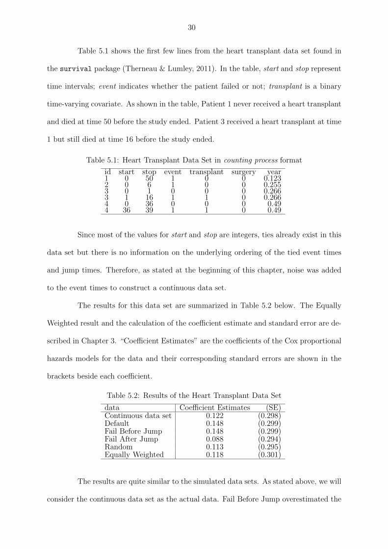
Table 5.1 shows the first few lines from the heart transplant data set found in
the survival package (Therneau & Lumley, 2011). In the table, start and stop represent
time intervals; event indicates whether the patient failed or not; transplant is a binary
time-varying covariate. As shown in the table, Patient 1 never received a heart transplant
and died at time 50 before the study ended. Patient 3 received a heart transplant at time
1 but still died at time 16 before the study ended.
Table 5.1: Heart Transplant Data Set in counting process format
id start stop event transplant surgery year1 0 50 1 0 0 0.1232 0 6 1 0 0 0.2553 0 1 0 0 0 0.2663 1 16 1 1 0 0.2664 0 36 0 0 0 0.494 36 39 1 1 0 0.49
Since most of the values for start and stop are integers, ties already exist in this
data set but there is no information on the underlying ordering of the tied event times
and jump times. Therefore, as stated at the beginning of this chapter, noise was added
to the event times to construct a continuous data set.
The results for this data set are summarized in Table 5.2 below. The Equally
Weighted result and the calculation of the coefficient estimate and standard error are de-
scribed in Chapter 3. “Coefficient Estimates” are the coefficients of the Cox proportional
hazards models for the data and their corresponding standard errors are shown in the
brackets beside each coefficient.
Table 5.2: Results of the Heart Transplant Data Set
data Coefficient Estimates (SE)Continuous data set 0.122 (0.298)Default 0.148 (0.299)Fail Before Jump 0.148 (0.299)Fail After Jump 0.088 (0.294)Random 0.113 (0.295)Equally Weighted 0.118 (0.301)
The results are quite similar to the simulated data sets. As stated above, we will
consider the continuous data set as the actual data. Fail Before Jump overestimated the
31
coefficient of the continuous data set; Fail After Jump underestimated it; Random and
Equally Weighted produced the coefficient estimates that are quite close to the coefficient
of continuous data.
The three percentages of Type 2 ties were calculated as described in Chapter 4.3:
Type 2 Jump = 17%, Type 2 Event = 13%, and Type 2 Total = 27%. The percentages
of Type 1 ties was found to be 22.3%. The percentages of both types of ties are smaller
than for the simulated data set as listed in Table 4.4 (In Table 4.4, the “Type 2 Total”
column is considered here).
5.2 SUD Data Set
The second data set is a record of 211 individuals that are at high risk of
getting psychiatric disorders since one of their parents has bipolar disorder or some similar
problem. In this data set, the time-scale is age and the start of observation is assumed
to be birth (age 0) for everyone. The important covariates in the data set are:
male: gender of the individuals; 1=male, 0=female;
SUD: Substance Abuse Disorder. SUD=1 if the individual is ever diagnosed with
Substance Abuse Disorder, 0 otherwise;
Age SUD: the age of the individual when SUD is diagnosed or missing (NA) if no
such diagnosis;
Age Last Assessment: the censoring variable;
MajMin: major or minor mood disorder. MajMin=1 if ever diagnosed with major
or minor mood disorder, 0 otherwise;
SES4 and SES5: social economic status (SES) level 4 and 5. SES4=1 if SESlevel=4,
0 otherwise; SES5=1 if SESlevel=5, 0 otherwise. If both SES4=SES5=0 then
32
SESlevel=1,2,or 3. SES5=1 if SESlevel=5, 0 otherwise. Higher values of SES level
mean higher income;
emotional: a score for emotionality. Higher value means the individual is more
emotional;
Age MajMin: age of major or minor mood diagnosis (whichever came first) or
missing (NA) if no such diagnosis.
The purpose of the study is to investigate how male, SES4, SES5, emotional
and the time of appearance of MajMin affect the risk of SUD. Therefore, SUD is the
event variable, male, SES4, SES5, emotional are the time-fixed covariates and a binary
time-varying covariate needs to be created for MajMin. This covariate is named MM in
this and the following sections. Out of the 211 patients, 104 individuals were diagnosed
with major or minor mood diagnosis before the study terminated, i.e., 104 individuals
experienced a change from 0 to 1 in the time-varying covariate MM. Fifty individuals
were diagnosed with SUD, i.e., had an event.
The values for time in the SUD data set are continuous. As discussed in the
beginning of this chapter, the original SUD data is the continuous data set, which has no
ties and so the ordering between events and jump times is known.
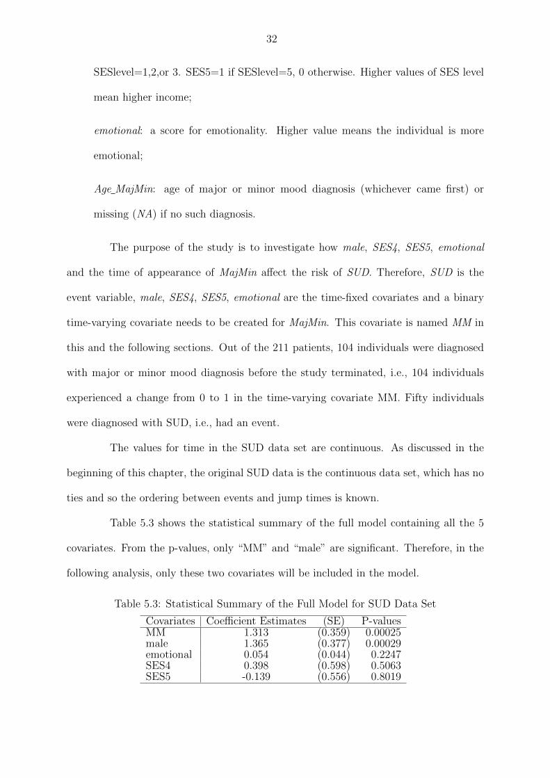
Table 5.3 shows the statistical summary of the full model containing all the 5
covariates. From the p-values, only “MM” and “male” are significant. Therefore, in the
following analysis, only these two covariates will be included in the model.
Table 5.3: Statistical Summary of the Full Model for SUD Data Set
Covariates Coefficient Estimates (SE) P-valuesMM 1.313 (0.359) 0.00025male 1.365 (0.377) 0.00029emotional 0.054 (0.044) 0.2247SES4 0.398 (0.598) 0.5063SES5 -0.139 (0.556) 0.8019
33
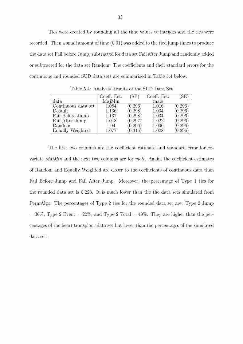
Ties were created by rounding all the time values to integers and the ties were
recorded. Then a small amount of time (0.01) was added to the tied jump times to produce
the data set Fail before Jump, subtracted for data set Fail after Jump and randomly added
or subtracted for the data set Random. The coefficients and their standard errors for the
continuous and rounded SUD data sets are summarized in Table 5.4 below.
Table 5.4: Analysis Results of the SUD Data Set
Coeff. Est. (SE) Coeff. Est. (SE)data MajMin maleContinuous data set 1.084 (0.296) 1.016 (0.296)Default 1.136 (0.298) 1.034 (0.296)Fail Before Jump 1.137 (0.298) 1.034 (0.296)Fail After Jump 1.018 (0.297) 1.022 (0.296)Random 1.04 (0.296) 1.006 (0.296)Equally Weighted 1.077 (0.315) 1.028 (0.296)
The first two columns are the coefficient estimate and standard error for co-
variate MajMin and the next two columns are for male. Again, the coefficient estimates
of Random and Equally Weighted are closer to the coefficients of continuous data than
Fail Before Jump and Fail After Jump. Moreover, the percentage of Type 1 ties for
the rounded data set is 0.223. It is much lower than the the data sets simulated from
PermAlgo. The percentages of Type 2 ties for the rounded data set are: Type 2 Jump
= 36%, Type 2 Event = 22%, and Type 2 Total = 49%. They are higher than the per-
centages of the heart transplant data set but lower than the percentages of the simulated
data set.
34
Chapter 6
Conclusions and Future Work
For the data set with only ties between event times and jump times in Table 2.5,
the three Cox proportional hazards models with exact method, Breslow Approximation
and Efron approximation produced exactly the same results. Therefore, it is verified that
these three methods only affect Type 1 ties but not Type 2 ties.
In the simulation study, the PermAlgo package worked well to generate survival
data with time-varying covariates. However, it can only generate integer time values.
To obtain the coefficient for the continuous data, noise needed to be added to the event
times so that there were no ties and time could be considered a continuous variable. The
data sets that are directly generated from PermAlgo can only be used as the rounded
data set but not the continuous data set.
It was discovered in this study that when fitting a Cox proportional hazards
model in SAS (SAS Institute Inc., 2010) and R (R Development Core Team, 2011),
Type 2 ties are automatically treated as if the event times occur before jump times, i.e.,
the Fail before Jump method. The results from both the simulated and real data sets
showed that Random and Equally Weighted produced coefficients that were close to the
true coefficient. Although Random always had a smaller standard error than Equally
Weighted, both the methods are appropriate for handling Type 2 ties.
However, the coefficient estimates of Random and Equally Weighted for the data
sets simulated from PermAlgo are not as close to the value of the continuous data as that
in the real data sets. The possible reason is that the Efron approximation deteriorates
35
as the percentage of Type 1 ties increases. It was shown that the percentages of both
Type 1 and Type 2 ties for all the simulated data sets are much higher than the heart
transplant data set and SUD data set.
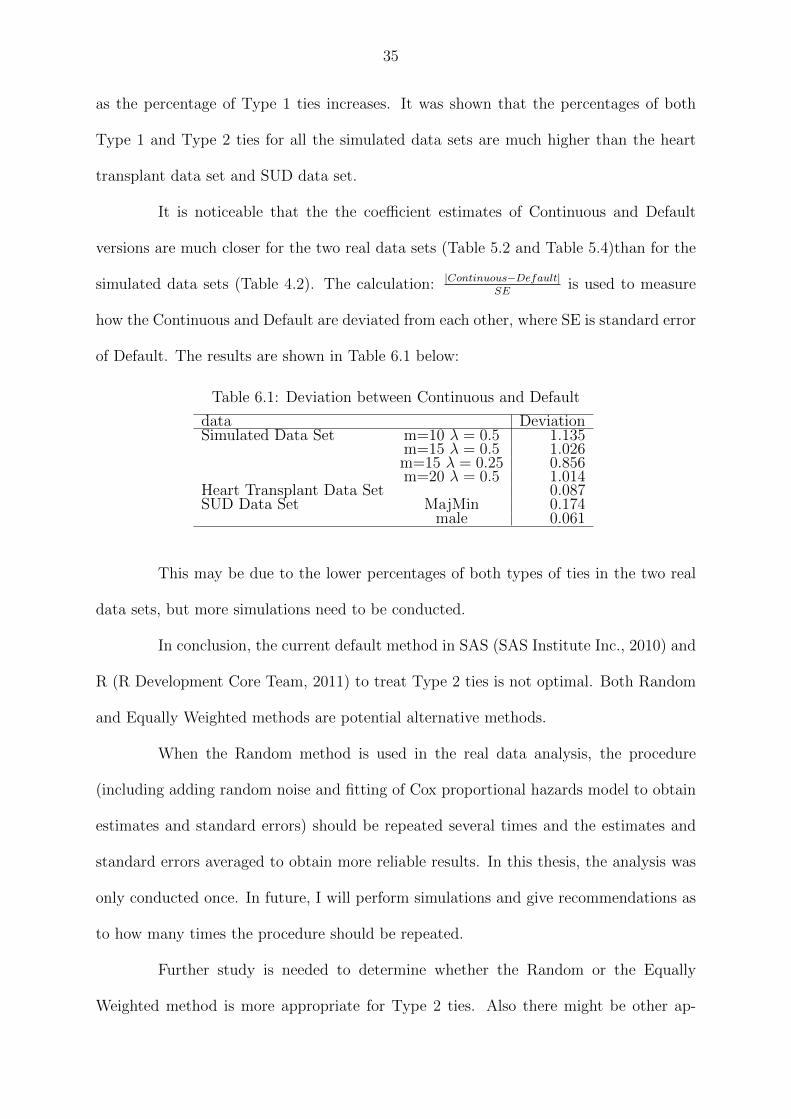
It is noticeable that the the coefficient estimates of Continuous and Default
versions are much closer for the two real data sets (Table 5.2 and Table 5.4)than for the
simulated data sets (Table 4.2). The calculation: |Continuous−Default|SE
is used to measure
how the Continuous and Default are deviated from each other, where SE is standard error
of Default. The results are shown in Table 6.1 below:
Table 6.1: Deviation between Continuous and Default
data DeviationSimulated Data Set m=10 λ = 0.5 1.135
m=15 λ = 0.5 1.026m=15 λ = 0.25 0.856m=20 λ = 0.5 1.014
Heart Transplant Data Set 0.087SUD Data Set MajMin 0.174
male 0.061
This may be due to the lower percentages of both types of ties in the two real
data sets, but more simulations need to be conducted.
In conclusion, the current default method in SAS (SAS Institute Inc., 2010) and
R (R Development Core Team, 2011) to treat Type 2 ties is not optimal. Both Random
and Equally Weighted methods are potential alternative methods.
When the Random method is used in the real data analysis, the procedure
(including adding random noise and fitting of Cox proportional hazards model to obtain
estimates and standard errors) should be repeated several times and the estimates and
standard errors averaged to obtain more reliable results. In this thesis, the analysis was
only conducted once. In future, I will perform simulations and give recommendations as
to how many times the procedure should be repeated.
Further study is needed to determine whether the Random or the Equally
Weighted method is more appropriate for Type 2 ties. Also there might be other ap-
36
proaches besides breaking the Type 2 ties. For instance, the exact method, the Efron
approximation, the Breslow approximation and the discrete methods can be developed
to treat both Type 1 and Type 2 ties. The effect of the percentages of Type 2 ties on the
methods proposed in this thesis should also be more fully investigated.
37
References
Abrahamowicz, M., Evans, T., MacKenzie, T. & Sylvestre, M.P. (2010). PermAlgo:
Permutational algorith to generate event times conditional on a covariate matrix
including time-dependent covariates. R package version 1.0.
Allison, P. (2010). Survival Analysis Using SAS: A Practical Guide. Cary, NC,
USA: SAS Institute Inc.
Breslow, N. (1974). Covariance analysis of censored survival data. Biometrics. 30,
89-99.
Crowley, J. & Hu, M. (1977). Covariance analysis of heart transplant survival data.
Journal of the American Statistical Association, 72, 2736.
Cox, D. R. (1972). Regression models and life-tables (with discussion). Journal of
the Royal Statistical Society. 34, 187-220.
DeLong, D. M., Guirguis, G. H., and So, Y. C. (1994). Efficient Computation of
Subset Selection Probabilities with Application to Cox Regression. Biometrika, 81,
607-611.
Duffy A., Horrocks, J., Milin, R., Doucette, S., Persson, G., Grof, P. (Submitted
June 30, 2011). Adolescent substance abuse in the development of bipolar disorder:
A prospective study. Journal of the American Academy of Child And Adolescent
Psychiatry.
Efron, B. (1977). The efficiency of Cox’s likelihood function of censored data.
Journal of the American Statistical Association. 72, 557-565.
Fox, J. (2002). Cox Proportional-Hazards Regression for Survival Data. Appendix
to An R and S-PLUS Companion to Applied Regression.
38
Hertz-Picciotto, I. & Rockhill, B. (1997). Validity and efficiency of approximation
methods for tied survival times in Cox regression. Biometrics, 53, 1151-1156.
Kalbfleisch, J. D. & Prentice, R. L. (1973). Marginal likelihoods based on Cox’s
regression and life model. Biometrika, 60, 267-278.
Kalbfleisch, J. D. & Prentice, R. L. (2002). The statistical analysis of failure time
data (2nd ed.). New York: John Wiley & Sons Inc.
Lawless, J.F. (2003). Statistical Models and Methods for Lifetime Data. New York:
John Wiley & Sons Inc.
Little, R.A. & Rubin, D.B. (1987). Statistical Analysis with Missing Data. New
York: John Wiley & Sons Inc.
R Development Core Team (2011). R: A Language and Environment for Statistical
Computing. R Foundation for Statistical Computing, Vienna, Austria. ISBN 3-
900051-07-0, URL http://www.R-project.org/.
SAS Institute Inc. 2010. SAS/GRAPH R© 9.2 Reference, Second Edition. Cary,
NC: SAS Institute Inc.
Therneau, T. & original Splus → R port by Lumley, T. (2011). survival: Survival
analysis, including penalised likelihood. R package version 2.36-9. http://CRAN.R-
project.org/package=survival.