A SURVEY OF SOME SLIDING MODE CONTROL DESIGNS

T. C. KUO

Overview

Most types of system control techniques incorporate some type of disturbance waveform modeling. Even if the disturbance waveform is completely unknown, a disturbance characterization of the waveform is assumed. This assumption is usually made on a worst case basis to insure stability of the targeted system.

Classical and Modern Control theory incorporates waveform characterization of disturbances with and without waveform structure. Modern control theory is centered around modeling the disturbance to either completely reject, minimize, or to even utilize the disturbance in controlling system behavior. In all of these circumstances it is necessary to model the waveform.

Some Waveform Models used in Modern Control Design

)()()(

)cos()sin()cos()sin()(

)()(

)()(

)()(

23

322

5

554321

2

2

21

2

2

21

tdtdw

dtwd

dtwd

tctctctcctw

tdtdw

dtwdecctw

tdt

wdtcctw

tdtdwctw

t

ωθφφθ

φφθθ

ωα

ω

σ

α

=+++→

++++=

=+→+=

=→+=

=→=

Introduction to Sliding Mode Control

Sliding Mode Control does not require a disturbance waveform characterization to implement the control law. The main advantage of Sliding Mode Control (SMC) is the robustness to unknown disturbances. Required knowledge of the disturbance is limited to the disturbance boundary. Traditional SMC was, however, limited by a discontinuous control law. Depending on the plant dynamics, high frequency switching may or may not be an issue to contend with. There are techniques to limit and eliminate the high-frequency switching associated with traditional SMC. It is the intent of this paper to look at several SMC techniques utilizing an aircraft model with bounded external disturbances.

Agenda

• Background of SMC• Definitions• SMC Design Methodology• Derivations

– Traditional SMC– Supertwist– SMC driven by SMC observer

• Simulation Results• Conclusions

Agenda

• Background of SMC••• DefinitionsDefinitionsDefinitions••• SMC Design MethodologySMC Design MethodologySMC Design Methodology••• DerivationsDerivationsDerivations

––– Traditional SMCTraditional SMCTraditional SMC––– SupertwistSupertwistSupertwist––– SMC driven by SMC observerSMC driven by SMC observerSMC driven by SMC observer

••• Simulation ResultsSimulation ResultsSimulation Results••• ConclusionsConclusionsConclusions

Background

• Sliding Mode Control (SMC) theory was founded and advanced in the former Soviet Union as a variable structure control system.

• SMC is a relatively young control concept dating back to the 1960s.

• SMC theory first appeared outside Russia in the mid 1970s when a book by Itkis (1976) and a survey paper by Utkin (1977) were published in English.

• The SMC “reachability” condition is based on the Russian mathematician, Lyapunov, and his theory of stability of nonlinear systems.

Agenda

••• Background of SMCBackground of SMCBackground of SMC• Definitions••• SMC Design MethodologySMC Design MethodologySMC Design Methodology••• DerivationsDerivationsDerivations

––– Traditional SMCTraditional SMCTraditional SMC––– SupertwistSupertwistSupertwist––– SMC driven by SMC observerSMC driven by SMC observerSMC driven by SMC observer

••• Simulation ResultsSimulation ResultsSimulation Results••• ConclusionsConclusionsConclusions

Definitions

• State Space – An n-dimensional space whose coordinate axes consist of the x1 axes,x2 axis,…,xn axes.

• State trajectory- A graph of x(t) verses t through a state space.

• State variables – The state variables of a system consist of a minimum set of parameters that completely summarize the system’s status.

• Disturbance – Completely or partially unknown system inputs which cannot be manipulated by the system designer.

Definitions

• Sliding Surface – A line or hyperplane in state-space which is designed to accommodate a sliding motion.

• Sliding Mode – The behavior of a dynamical system while confined to the sliding surface.

• Signum function (Sign(s)) –

• Reaching phase – The initial phase of the closed loop behaviour of the state variables as they are being driven towards the surface.

⎩⎨⎧

<−>+

0),(10),( 1

yy if syysif&

&

Agenda

••• Background of SMCBackground of SMCBackground of SMC••• DefinitionsDefinitionsDefinitions• SMC design Methodology••• DerivationsDerivationsDerivations

––– Traditional SMCTraditional SMCTraditional SMC––– SupertwistSupertwistSupertwist––– SMC driven by SMC observerSMC driven by SMC observerSMC driven by SMC observer

••• Simulation ResultsSimulation ResultsSimulation Results••• ConclusionsConclusionsConclusions

SMC Design MethodologyThree Basic Steps

• Design a sliding manifold or sliding surface in state space.

• Design a controller to reach the sliding surface in finite time.

• Design a control law to confine the desired state variables to the sliding manifold.

SMC Graphical Illustration

Agenda

••• Background of SMCBackground of SMCBackground of SMC••• DefinitionsDefinitionsDefinitions••• SMC design MethodologySMC design MethodologySMC design Methodology• Derivations

– Traditional SMC– Supertwist– SMC driven by SMC observer

••• Simulation ResultsSimulation ResultsSimulation Results••• ConclusionsConclusionsConclusions

Aircraft Modeled Parameters

• Simplified aircraft model consist of angle of attack, aircraft pitch rate, and elevator deflection represented as α ,q, and δe.

• Aircraft parameters for a particular airframe at a particular attitude and altitude.

• Changes in airframe due to damage (unknown, uncertain, and bounded)

• Horizontal tail and rudder areas.

• Flight profile filters.

≡ΔA

≡nA

≡B

≡*αα c

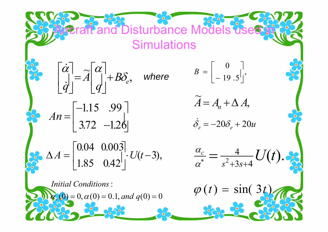
Aircraft and Disturbance Models used in Simulations

uee 2020 +−= δδ&

, ~eB

qA

qδ

αα+⎥⎦

⎤⎢⎣

⎡=⎥⎦

⎤⎢⎣

⎡&

&

, ~ AAA n Δ+=⎥⎦

⎤⎢⎣

⎡−

−=

26.172.399.15.1

An

),3(42.085.1003.004.0

−⋅⎥⎦

⎤⎢⎣

⎡=Δ tUA

,5.19

0⎥⎦

⎤⎢⎣

⎡−

=Bwhere

).(43

42 tU

ssc

++=∗α

α

)3sin()( tt =ϕ0)0( ,1.0)0( ,0)0(

: === qand

ConditionsInitial

c αα

Derivations for Traditional SMC

• It is necessary to find the relative degree of the system in state-space. Relative degree, , is determined by the number of times the output has to be differentiated before any control input appears in its expression.

• The aircraft model in scalar format is:

• The relative degree of the plant is 3 as the control u appears as follows:

eqqq

δααα

5.1926.172.399.015.1−−=

+−=&

&

Γ

buhgqfy e +++== δαα&&&&&&

α=yuee 2020 +−= δδ&

Sliding Surface Design

The sliding manifold is formulated as:where

then .and are deigned to make the dynamic

sliding surface stable. This is achieved by making the equation Hurwitz stable. The equation from the ITAE tables for a 2nd order system is:

and for a then C1 and C2 are 14 and 100 respectively.

eCeCenn

2

1

1 ++=−

σ 1−Γ=neCeCe 21 ++= &&&σ

1C 2C

10=nW

22 4.1 nn wsws ++

Derivation for reaching phase

To guarantee an ideal sliding motion the ‘ρ-reachability’condition must be met and is given by

ρσ

ρσρσσ

ρσσ

ρσρσ

ρσρσσσσ

σ

)0( :by σ(0)any for satisfied is

condition ty reachabili thezero toσ settingBy

)0()0(

)0()0()(

dt

0

)(

)0(

≤

=→−=→

−−=−→

−=→−=

−≤→−≤

∫∫

r

r

tt

t

tt

tt

dtddthen

&&

constant. positive smalla is ρσρσσ where−≤&

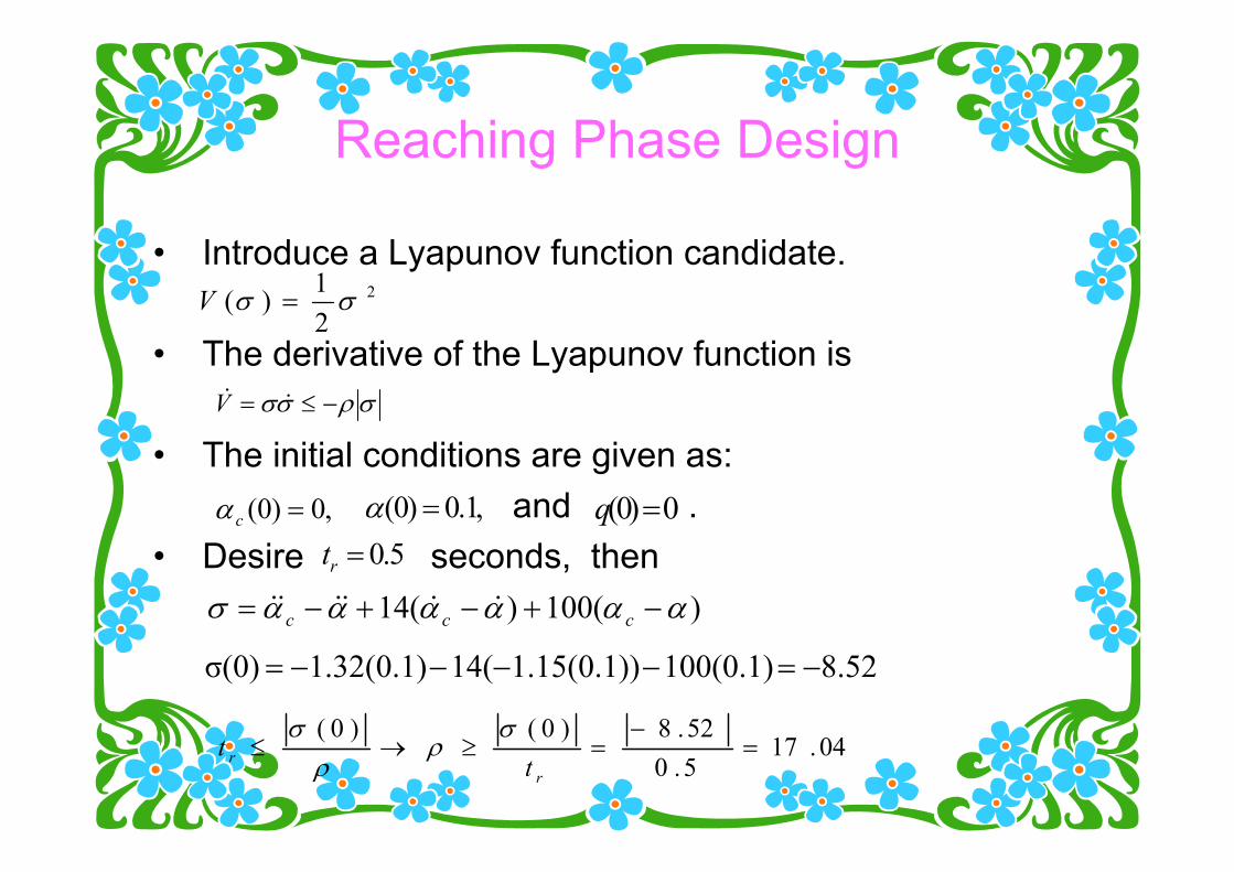
Reaching Phase Design

• Introduce a Lyapunov function candidate.

• The derivative of the Lyapunov function is

• The initial conditions are given as:and .

• Desire seconds, then

04.175.052.8)0()0(

=−

=≥→≤r

r tt

σρ

ρσ

σρσσ −≤= &&V

2

21)( σσ =V

,1.0)0( =α 0)0( =q,0)0( =cα

8.52100(0.1)1.15(0.1))14(1.32(0.1)σ(0) −=−−−−=

5.0=rt

)(100)(14 αααααασ −+−+−= ccc &&&&&&

SMC Controller Design

• The controller can be implemented with the signum function as follows:

( ) )(σρ signLu +−=

)3sin( tL ≥ .5.1let 1 ≈≥ LL

04.175.052.8 =≥ρ

)(5.18 σsignu −=

Simulink Diagram for Traditionial SMC

Supertwist Design

It has been shown (not in this brief) that the solution to the following differential equation

and its derivative converge to zero in finite time if, , and .

On this basis u is introduced as:

σσβσσα dsignsignu )()(2/1∫+=

L2/1≥α L4≥β Lt ≤)(ξ

)()()(2/1 tdzsignzsignzz ξτβα =++ ∫&

Supertwist Design

• Supertwist utilizes the same sliding surface and values as the traditional SMC. The signumcontrol function is replaced with the function:

• The values for L=1.5 are:

σσβσσα dsignsignu )()(2/1∫+=

L2/1≥α L4≥β

612.5.12/1 =≥α

,6)5.1(4 =≥β

Supertwist Block Diagram

SMC Observer Design

.ˆ )(

)3( ))(())(( :yields )(

with ˆ ngsubstituti and Eq(2) of inequality the to(1) Eq. Applying(2) 0ˆ,ˆ(1) )(

)(:yields solving and into ngsubstituti and atingDifferenti

:follows as

designed is and as introduced is variableslidingauxiliary newA ˆ0 11

ρρϕ

ϕ

ρρρ

ϕϕσ

σ

ϕϕϕ

+≥≤⋅

+≤+⋅=

+

>−<

+⋅=+−+⋅=+=

+−=+=

⋅=>+=+⋅=→=+⋅=

LandLwhere

swsignLswsssswsignL

sssws

wvvzszs

wvzandzs

s)( and v, Kv-Kσv

v where)(σv, bu, bu)(σ

&

&

&

&&&

&

&

&&

SMC Observer Design

).(ˆobtain filter to pass-low a of meansby filter tonecessary isit of switchingfrequency -high theremove To

).( and0 surface sliding in the mode sliding theof existance indicates which Eq.(3) as same theis which ˆ)ss( ˆ))(s(

thenˆˆ)(

))( ˆ( )ˆ)((then

(4) ˆ:asselected is SMCIf

eq ⋅−=

⋅==

−≤→−≤+⋅

−≤+−⋅

+≤+⋅

+=

ϕ

ϕϕ

ϕ

ϕ

www

w ssρsρw

sρ)sign(s)) ρ(Ls(

ssign)sign(s)ρL-(Ls)sign(s)ρ-(Ls

)sign(s)ρ-(Lww

eq

&

Disturbance Observer Block Diagram

Agenda

••• Background of SMCBackground of SMCBackground of SMC••• DefinitionsDefinitionsDefinitions••• SMC design MethodologySMC design MethodologySMC design Methodology••• DerivationsDerivationsDerivations

––– Traditional SMCTraditional SMCTraditional SMC––– SupertwistSupertwistSupertwist––– SMC driven by SMC observerSMC driven by SMC observerSMC driven by SMC observer

• Simulation Results••• ConclusionsConclusionsConclusions

Disturbances

Phase Diagramof the Sliding Surface

Traditional SMC

Supertwist

SMC Observer

Agenda

••• Background of SMCBackground of SMCBackground of SMC••• DefinitionsDefinitionsDefinitions••• SMC design MethodologySMC design MethodologySMC design Methodology••• DerivationsDerivationsDerivations

––– Traditional SMCTraditional SMCTraditional SMC––– SupertwistSupertwistSupertwist––– SMC driven by SMC observerSMC driven by SMC observerSMC driven by SMC observer

••• Simulation ResultsSimulation ResultsSimulation Results• Conclusions

Conclusion and Comments

• Traditional SMC.– High frequency switching controller.– Simple controller design.– High quality control.

• Supertwist – Continuous control function.– Controller is more complex.– High quality control.

• Disturbance SMC Driven by SMC Observer– Continuous controller.– More complex than supertwist.– Very high quality control.

• All SMC designs provided high quality of control without disturbance waveform modeling.

Summary

• Reviewed some background and definitions related to SMC.

• Derived three types of sliding mode controllers, traditional, Supertwist, and SMC Driven by a SMC Observer.

• Simulated each controller in Simulink using a partial plant model of a F-16 aircraft.

• Simulated a phase portrait of the sliding surface in state space.

• Compared simulation results of the error and control output for each design.

References

• Shtessel, Y., Buffington, J., and Banda, S.”MultipleTimescale Flight Control Using Reconfigurable Sliding Modes, “Journal of Guidance, Control, and Dynamics”,Vol. 22, No. 6, Nov. Dec. 1999, pp. 873-883

• Edwards, Christopher, and Surgeon, Sarah, K. “Sliding Mode Control, Theory and Applications”, Taylor and Frances Inc., 1900 Frost Road, Suite 101, Bristol, PA 19007

• Brogan, William, L. “Modern Control Theory”, Third edition, Prentice Hall, Englewood Cliffs, New Jersey 07632

• Dorf, Richard, C., and Bishop, Robert, H, “Modern Control Systems”, Ninth edition, Prentice Hall, Upper Saddle River, NJ 07457