Embed Size (px)
Citation preview
Nonlinear Course
Professor : Dr. H.Taghirad
Winter 2008
A Survey on Singularly Perturbed Systems
Nima Monshizadeh
Abstract:
Multiple time-scale phenomena are almost unavoidable in real systems and the
singular perturbation approach has proven to be a powerful tool for system analysis
and control design. Singular perturbation theory has received a lot of attention in the
past decades.
In this article, first the concept of perturbation and singular perturbation are studied.
Then the related theories and analysis followed by some chosen examples are given in
some details. Note that discussions given in the solution of these examples are mainly
according to my personal understanding and perception and therefore it might have
some deficiencies and imperfections. At the next chapter, the recent work in around
30 journal papers have been categorized due to their subject. This chapter will
addresses those who want to research in this area to the useful papers. Moreover, for
some of these papers, the concept of the proposed methods is discussed. In section
2.3, some applications regard to singular perturbation problem is mentioned. Finally a
typical example has been simulated and the obtained results are discussed.
Introduction:
Exact closed-form analytic solutions of nonlinear differential equations are possible
only for a limited number of special classes of differential equations.
There for we have to resort to approximate methods.
Suppose we are given the state equation:
),t,x(fx ε=•
Where ε is a small scalar parameter and, under certain conditions, the equation has
an exact solution ),t(x ε . We want to find an approximate solution such that
the approximation error is negligible for small
),t(x~
ε
),t(x),t(x~
εε − ε . Moreover it is
evident that to make our original problem easier, the approximated solution
must be expressed in terms of equations simpler than the original equation.Quite
often, the solution of the state equation exhibits the phenomenon that some variables
move in time faster than other variables, leading to the classification of variables as
“slow” and “fast”. If the state equations depend smoothly on parameter
),t(x~
ε
ε , then the
approximated method can be achieved through the regular perturbation and averaging
method, while in the singular perturbation problem, we face a more difficult
perturbation problem characterized by discontinuous dependence of system properties
on the perturbation parameterε , which involves more coupling between the fast and
slow modes of system.
CHAPTER 1:
Singular Perturbation Method:
1.1 Introducing the Standard Singular Perturbation model:
Let x denote the “slow” variables and z denote the fast ones, then the standard
singular perturbation problem are stated as follows:
),,z,x,t ( g z ),,z,x , t ( f x εε
ε= ×
= •
•
z )2.1()1.1(x
m
n
ℜ∈ℜ∈
We assume f and g are continuously differentiable in their arguments.
We see that setting ε to zero, causes an abrupt change in dynamic properties of the
system and the dimensions of state equations reduces from n+m to n.
Thus, the differential equation (1.2) will change to:
)3.1(),z,x,t(g0 ε=
Let us show the roots of this equation by
)4.1(k,...,1,1i),x,t(hz i ==
With assumption of isolated real roots, we have k reduced model that each one
corresponds to the related root. If we substitute the (1.4) into (1.1), we have:
)5.1()0),x,t(h,x,t(fx i=•
Since a small value of ε leads to the fast convergence of z to a root of (1.3)
(which is the equilibrium of (1.2).) , this equation is sometimes called a quasi-steady-
state model. On the other hand, since (1.5) deals with the slow variables x, this model
is also known as the slow model.
1.2 Singular Perturbation Modelling
Converting physical model into the standard singular perturbation problem is not
usually easy. The choice of state variables and choice of ε require a careful thought.
Sometimes we can model the parasitic terms like small time constants, masses,
capacitors… through singular perturbation form. These mentioned terms are usually
ignored in the simplified model. Thus singular perturbation provides us a tool for
modelling these extra terms in some over-simplified models. Let us analyze some
chosen examples (from [1]) to see how to model a problem into singular perturbation
form.
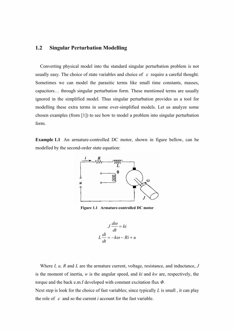
Example 1.1 An armature-controlled DC motor, shown in figure bellow, can be
modelled by the second-order state equation:
Figure 1.1 Armature-controlled DC motor
uRikdtdiL
kidtdJ
+−−=
=
ω
ω
Where I, u, R and L are the armature current, voltage, resistance, and inductance, J
is the moment of inertia, w is the angular speed, and ki and kw are, respectively, the
torque and the back e.m.f developed with constant excitation flux Φ.
Next step is look for the choice of fast variables; since typically L is small , it can play
the role of ε and so the current i account for the fast variable.
In singular perturbation modelling it is preferable to have dimensionless state
variables and perturbation parameters. Therefore it is suitable to normalize the above
system equations. The new system equations can be represented as:
rrrr
e
rr
m
uidtdiT
idt
dwT
+−−=
=
ω
Where Tm and Te are mechanical and electrical time constants respectively.
In the above equations the state variables are dimensionless but the perturbation
parameter Te ( Te<< Tm ) is still have dimension. It can be seen that if we let Tm to be
the time unit ( m
r Ttt = , then
m
e
TT is a dimensionless parameter which can play the
role ofε . Therefore we can rewrite the normalized system equations in the following
form:
rrrr
m
e
rr
r
uidtdi
TT
idtd
+−−=
=
ω
ω
Now assuming m
e
TT as ε , the above equation is in the form of standard singular
perturbation problem. Setting ε to zero leads to the equation:
ui0 rr +−−= ω .
To obtain the reduced model as we discussed earlier we should substitute the root
of this equation into the torque equation, thus we obtain the quasi-steady-state model :
rrr
r udtd
−= ωω
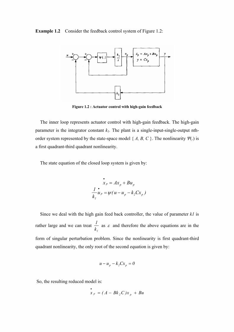
Example 1.2 Consider the feedback control system of Figure 1.2:
Figure 1.2 : Actuator control with high-gain feedback
The inner loop represents actuator control with high-gain feedback. The high-gain
parameter is the integrator constant k1. The plant is a single-input-single-output nth-
order system represented by the state-space model { A, B, C }. The nonlinearity Ψ(.) is
a first quadrant-third quadrant nonlinearity.
The state equation of the closed loop system is given by:
)Cxkuu(uk1
BuAxx
p2pp
1
ppp
−−=
+=•
•
ψ
Since we deal with the high gain feed back controller, the value of parameter k1 is
rather large and we can treat 1k
1 as ε and therefore the above equations are in the
form of singular perturbation problem. Since the nonlinearity is first quadrant-third
quadrant nonlinearity, the only root of the second equation is given by:
0Cxkuu p2p =−−
So, the resulting reduced model is:
Bux)CBkA(x p2p +−=•
This result is also evident form the figure 1.2 : setting ε to zero is the same as
assuming k1 to have infinity value. This value causes the inner loop to behave like a
constant gain equal to1. Therefore the simplified model is given by
BuyBkAxx 2pp +−=•
Which corresponds to the pervious answer since pCxy = .
1.2 Singular Perturbed System Analysis:
In the pervious section we have somehow learned how to model a typical physical
problem into a singular perturbation model.
We have discussed that the singular perturbation model includes two categories of
slow and fast variables. The reduced model actually ignores the fast transient response
and is related to the slow response of the system. Recall that we have set ε to zero to
obtain the reduced model. But, having set the ε to zero, will make the fast variable z
instantaneous, and there is no guarantee for the convergence of z to its quasi-steady-
state. This convergence must be hold for the validity of our simplified model.
To skip some boring mathematical analysis let us consider this concept through an
example:
Example 1.3 Consider the singular perturbation problem for the DC motor of
example 1.1:
0
0
)0(z)t(uzxz
)0(xzx
ηε
ξ
=+−−=
==•
•
Suppose u(t) = t for t > 0 and we want to solve the state equation over the interval
[0, 1] .
The unique root of the fast state variable equation is:
tx)t(ux)x,t(h +−=+−= .
To obtain the reduced model as we said earlier we should substitute the root
into the slow state variable equation, Thus we have the reduced model as:
)x,t(h
0)0(xtxx ξ=+−=•
.
Since we want to analyze the convergence of the fast variable z to its quasi-steady-
state, it is quite suitable to shift this quasi-steady-state (i.e. h(t,x) ) to the origin. To
do this task, we define new variable y such that )x,t(hzy −= .
As a result the new system equations obtained as follows:
zxh
th)t(u)x,t(hyxy)t(u))x,t(hy(x))x,t(hy(
)x,t(hyx
∂∂
−∂∂
−+−−−=⇒++−−=+
+=
•••
•
εεεε
With the initial state:
00
0
)0(y
)0(x
ηξ
ξ
+=
=
As we discussed earlier due to the presence of fast and slow states, singular
perturbation shows multi-time scale behaviour, therefore it seems appropriate that we
analyze the slow and fast state variables in different time scale. Let us define the new
time-scale τ for the analysis of the fast transient dynamic. Note that we want to have
a better view of what is happening for the fast transient, on the other hand all the
events related to the fast transient occurs at a quite small interval after t0 . Therefore
the time-axis should be stretched so that we can see these events much more clear. As
a result we define: ε
τ )tt( 0−=
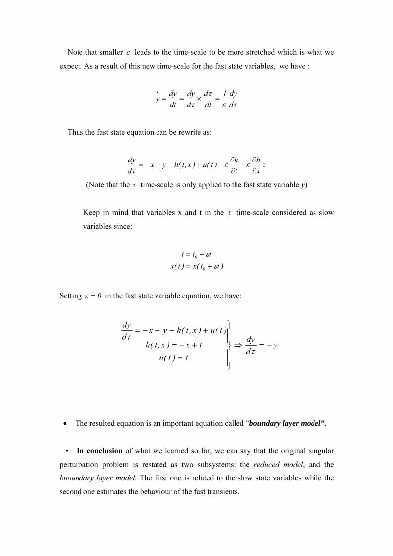
Note that smaller ε leads to the time-scale to be more stretched which is what we
expect. As a result of this new time-scale for the fast state variables, we have :
τετ
τ ddy1
dtd
ddy
dtdyy =×==
•
Thus the fast state equation can be rewrite as:
zxh
th)t(u)x,t(hyx
ddy
∂∂
−∂∂
−+−−−= εετ
(Note that the τ time-scale is only applied to the fast state variable y)
Keep in mind that variables x and t in the τ time-scale considered as slow
variables since:
)tt(x)t(xttt
0
0
εε+=
+=
Setting 0=ε in the fast state variable equation, we have:
yddy
t)t(utx)x,t(h
)t(u)x,t(hyxddy
−=⇒
⎪⎪⎭
⎪⎪⎬
⎫
=+−=
+−−−=
τ
τ
• The resulted equation is an important equation called “boundary layer model”.
• In conclusion of what we learned so far, we can say that the original singular
perturbation problem is restated as two subsystems: the reduced model, and the
bnoundary layer model. The first one is related to the slow state variables while the
second one estimates the behaviour of the fast transients.
In our example we obtained these mentioned two models as:
⎪⎩
⎪⎨
⎧
+=−=
=+−=
00
0
)0(yyddy
)0(xtxdtdx
ηξτ
ξ
The reduced model response is:
t0
~e)1()1t()t(x −++−= ξ
The boundary layer system is globally exponentially stable and its response is:
τηξτ −+= e)()(y oo
~.
Therefore the approximate response of our original variable z would be equal to :
t0
t
oo
~~~~e)1(1e)()t(z)x,t(h)t(y)t(z −−
+−++=⎯→⎯+= ξηξ ε
We can see from the above result that the approximation of the fast state variable ,
starts form the boundary layer and rapidly converges to the reduced model.
~z
• Generally the reduced and boundary model can be obtained by the following
equations:
)7.1()0),x,t(hy,x,t(gddy
)6.1()0),x,t(h,x,t(fdtdx
+=
=
τ
1.4 Geometric view of Singular Perturbation Problem:
In this section we want to give a geometric view of the singular perturbation
problem including reduced and boundary model. First it is necessary to get familiar
with the concept of Integral Manifold.
Integral Manifold ( Invariant Manifold ) :
Consider the following differential equation:
)8.1()X,t(Nx =•
where . The set is said to be an integral manifold if for
, the solution
nN,X ℜ∈ nℜ×ℜ⊂Μ
Μ∈∀ )X,t( 00 00 X)t(X)),t(x,t( = , is in Μ , for all . ℜ∈t
If only for a finite interval of time, Μ∈))t(x,t( , then M is said to be a local integral
manifold.
This definition implies that if the initial state start on Μ the trajectories of the
system remains in Μ thereafter.
Now, let us illustrate the geometric view of our singular perturbation problem
through a simple example:
Example 1.4 Consider the singular perturbed system :
)xz1(tanz
zxx
1 −−=
+−=
−•
•
ε
The second equation has the isolated root equal to : )x1(z −= . This equation
represents a one-dimensional manifold in , this manifold is considered as the 2ℜ
slow manifold, since it refers to the reduced ( slow ) model. The corresponding slow
model is obtained by : , which has an asymptotically stable equilibrium
point P = (1/2,1/2). Therefore if the trajectories start on this slow manifold it would
exponentially converges to point P and so this manifold also represents an integral
manifold.
1x2x +−=•
In order to have a overall view of the phase plane of the system I think it is helpful
to look into the ratiodzdx . This ratio can be reconsidered as:
)9.1()z,x(g
)z,x(f
dtdzdtdx
dzdx ×
==ε
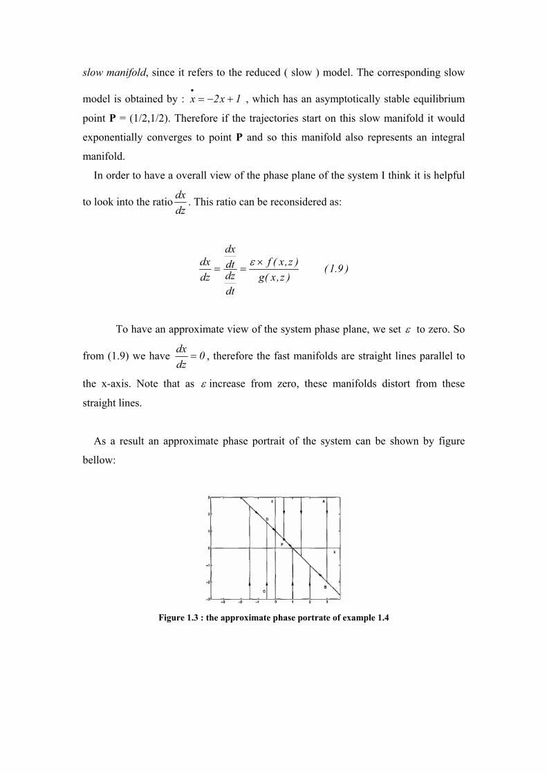
To have an approximate view of the system phase plane, we set ε to zero. So
from (1.9) we have 0dzdx
= , therefore the fast manifolds are straight lines parallel to
the x-axis. Note that as ε increase from zero, these manifolds distort from these
straight lines.
As a result an approximate phase portrait of the system can be shown by figure
bellow:
Figure 1.3 : the approximate phase portrate of example 1.4
It is useful to look at the boundary layer model in this problem:
According to (1.7) the boundary layer model is:
)y(tan)y(tanddy 11 −− −=−=τ
Form the above equation we can see that when the ( ) then 0y > )x,t(hz >
0ddy
<τ
. Consequently the variable y decreases and the fast variable z converges to
h(t,x) along the fast manifold. This is the case when in figure 1.5 the trajectories start
from a point above the line 1xz +−= .
When (0y < )x,t(hz < ) then 0ddy
>τ
. Consequently the variable y increases and
the fast variable z converges to h(t,x) along the fast manifold. This is the case when in
figure 1.3 the trajectories start from a point over the line 1xz +−= .
When the trajectory start on the line 1xz +−= then 0ddy0y =⎯→⎯=τ
and the
trajectory does not distort from the line and converges to the equilibrium point
according to the reduced model equation: . 1x2x +−=•
1.5 Stability Analysis :
Here, we devote our attention to one of the theories in this field that has an
extremely important concept. This theory verifies the robustness of exponential
stability to the unmodeled fast dynamics. This theory also relates the stability of
reduced model and boundary layer model to the whole (actual) system stability.
Theorem: Consider the singularly perturbed system:
),z,x,t(gz
),z,x,t(fx
εε
ε
=
=
•
•
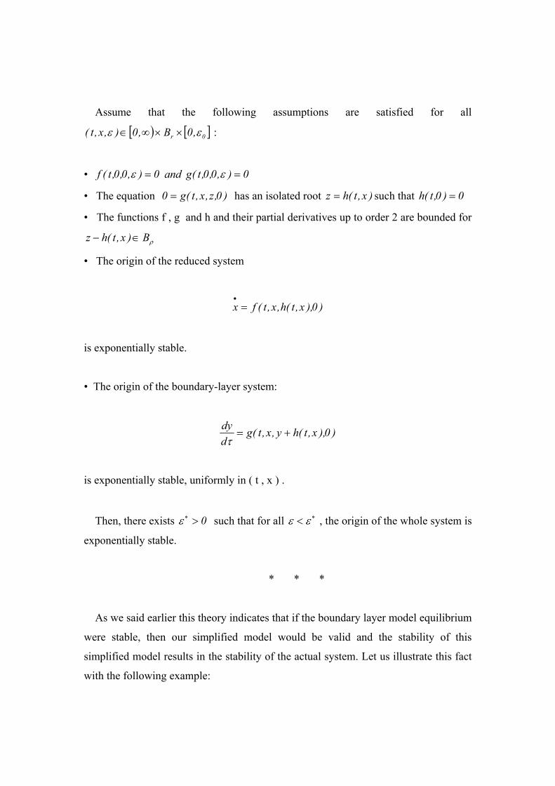
Assume that the following assumptions are satisfied for all
[ ) [ ]0r ,0B,0),x,t( εε ××∞∈ :
• 0),0,0,t(f =ε and 0),0,0,t(g =ε
• The equation )0,z,x,t(g0 = has an isolated root )x,t(hz = such that 0)0,t(h =
• The functions f , g and h and their partial derivatives up to order 2 are bounded for
ρB)x,t(hz ∈−
• The origin of the reduced system
)0),x,t(h,x,t(fx =•
is exponentially stable.
• The origin of the boundary-layer system:
)0),x,t(hy,x,t(gddy
+=τ
is exponentially stable, uniformly in ( t , x ) .
Then, there exists such that for all , the origin of the whole system is
exponentially stable.
0>∗ε ∗< εε
* * *
As we said earlier this theory indicates that if the boundary layer model equilibrium
were stable, then our simplified model would be valid and the stability of this
simplified model results in the stability of the actual system. Let us illustrate this fact
with the following example:
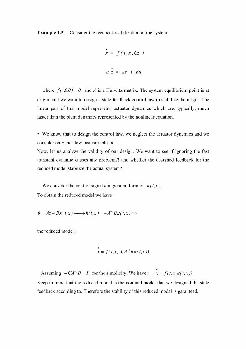
Example 1.5 Consider the feedback stabilization of the system
BuAzz
)Cz,x,t(fx
+=
=
•
•
ε
where 0)0,0,t(f = and A is a Hurwitz matrix. The system equilibrium point is at
origin, and we want to design a state feedback control law to stabilize the origin. The
linear part of this model represents actuator dynamics which are, typically, much
faster than the plant dynamics represented by the nonlinear equation.
• We know that to design the control law, we neglect the actuator dynamics and we
consider only the slow fast variables x.
Now, let us analyze the validity of our design. We want to see if ignoring the fast
transient dynamic causes any problem?! and whether the designed feedback for the
reduced model stabilize the actual system?!
We consider the control signal u in general form of )x,t(κ .
To obtain the reduced model we have :
⇒−=⎯→⎯+= − )x,t(BA)x,t(h)x,t(BAz0 1 κκ
the reduced model :
))x,t(BCA,x,t(fx 1 κ−•
−=
Assuming for the simplicity, We have : IBCA 1 =− − ))x,t(,x,t(fx κ=•
Keep in mind that the reduced model is the nominal model that we designed the state
feedback according to. Therefore the stability of this reduced model is garanteed.
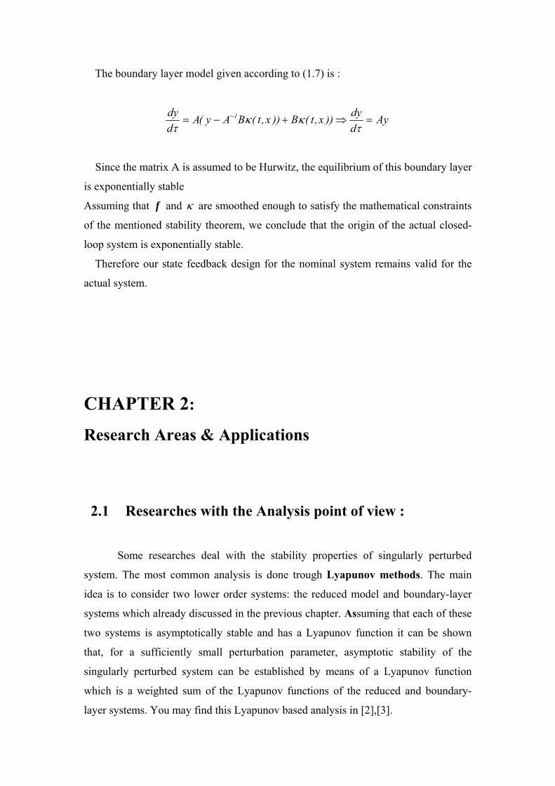
The boundary layer model given according to (1.7) is :
Ayddy))x,t(B))x,t(BAy(A
ddy 1 =⇒+−= −
τκκ
τ
Since the matrix A is assumed to be Hurwitz, the equilibrium of this boundary layer
is exponentially stable
Assuming that f and κ are smoothed enough to satisfy the mathematical constraints
of the mentioned stability theorem, we conclude that the origin of the actual closed-
loop system is exponentially stable.
Therefore our state feedback design for the nominal system remains valid for the
actual system.
CHAPTER 2:
Research Areas & Applications
2.1 Researches with the Analysis point of view :
Some researches deal with the stability properties of singularly perturbed
system. The most common analysis is done trough Lyapunov methods. The main
idea is to consider two lower order systems: the reduced model and boundary-layer
systems which already discussed in the previous chapter. Assuming that each of these
two systems is asymptotically stable and has a Lyapunov function it can be shown
that, for a sufficiently small perturbation parameter, asymptotic stability of the
singularly perturbed system can be established by means of a Lyapunov function
which is a weighted sum of the Lyapunov functions of the reduced and boundary-
layer systems. You may find this Lyapunov based analysis in [2],[3].
Furthermore, in [3] this composite Lyapunov function is used it to obtain estimates
of the domain of attraction. The method given in [3] is however limited to a special
case where the boundary-layer system is linear.
In [4] a general case in which the boundary-layer system is also nonlinear is studied
and in addition to stability analysis, the quadratic-type composite Lyapunov function
is used to obtain an upper bound on the perturbation parameter and also to estimate
the domain of attraction. It is also shown that the choice of the weights of the
composite Lyapunov function involves a trade off between obtaining a large estimate
of the domain of attraction and a large upper bound on the perturbation parameter. ε
In [10] an alternative stability analysis can be found: A kind of LFT form of the
singular perturbed system has been proposed. Using linear fractional transformations,
a singularly perturbed system is formulated into a standard μ - interconnection
framework. Also a set of new stability conditions for the system by defining the real
structured singular value μ is derived. Note that this method is only limited to linear
singular perturbed system.
• Those who are interested in Lur’se problem can find the circle criterion for the
singular perturbed system in [11].
*************************************************
The stability analysis and stability properties of the Time Delayed Singularly
Perturbed System is one of the interesting research subjects in the field of singular
perturbed system. A small delay in the feedback loop of a singularly perturbed system
may destabilize it; however, without the delay, it is stable for all small enough values
of a singular perturbation parameter.
In [5] the stability of a linear time invariant singularly perturbed system with time-
delay in slow states is discussed. An upper bound for perturbation parameter is
given, such that the stability of the full-order system can be inferred from the analysis
∗ε
of the reduced-order model in separate time scales. It also provided a way to find the
range for time delay such that the stability of the system is guaranteed for . ∗<≤ εε0
• Generally two main approaches have been developed for the treatment of the
effects of small delays: frequency domain techniques and direct analysis of
characteristic equation. The stability of singularly perturbed systems with delays in
the frequency domain can be found in [6] and [7].
However, the method of LMIs is more suitable for robust stability of systems with
uncertainties and for other control problems. (see e.g. [8]).
In [9] sufficient and necessary conditions for preserving stability, for all small
enough values of delay and ε , are given in two cases: in the case of delay
proportional to ε and in the case of independent delay and ε . Also the sufficient
conditions are given in terms of an LMI for the second case.
2.2 Design Methods :
2.2.1 Linear Singular Perturbed System:
• Optimum Control Design:
Consider the problem of finding the optimal state feedback gains solving the linear-
quadratic regulator (LQR) problem for the following singularly perturbed linear, time-
invariant system:
2211
22221212
12121111
xCxCy
uBxAxAx
uBxAxAx
+=
++=
++=
•
•
ε
The above system is said to be in standard form if A22 is invertible. There are
generally three representative options for solving
this problem :
(1) The special structure of the above system may be ignored, and the full
regulator algebraic Riccati equation (ARE) is solved.
This method leads to numerical difficulties. Further, we will have missed the chance
to reduce the size and complexity of our controller which is a particularly important
consideration for large systems. (see e.g. [11]).
(2) The second method is related to what we have illustrated in the previous
chapter: transforming the actual system into two subsystems, the reduced model and
the boundary layer model. Then the Regulator AREs are solved independently for
these two subsystems to obtain slow and fast feedback gains, sΚ and fΚ .Then the
composite control ffss xxu ΚΚ += an approximation of the true optimal value. (see
e.g. [12]).
This is a valuable result since two smaller computations are preferred to a single
large one, and also the resulting compensator complexity is reduced. However, the
near optimality of the solution (and even stability) is guaranteed asymptotically, only
for sufficiently smallε .
• The extension of this design method into Non-standard case where A22 is not
invertible is discussed in [15].
• In [16] considering the reduced model and boundary layer model, the output
feedback design is discussed in the discrete singular perturbed system.
(3) In this method first we construct the Hamiltonian form of the optimal
closed-loop system, with new slow states consisting of x1 and the slow co-states, and
new fast states consisting of x2 augmented by the fast co-states. Their results are
motivated and enabled by the observation that the Hamiltonian system maintains its
Hamiltonian structure under the exact decoupling transformation.
Manipulation of the decoupled pure-slow and pure-fast Hamiltonian systems results
again in two AREs, which may be solved for the pure-slow and pure-fast state
feedback gains. This approach differs from the second method in two important ways:
The first is that the corresponding composite control in this approach is exactly the
optimal control. The second is that the decoupled regulator
AREs are non-symmetric. (see e.g. [13])
• The above methods were about the time-invariant system. In [14] a new method is
proposed for the time-varying case.
*************************************************
• Control problem for singularly perturbed systems has been extensively
studied in the 90s . (see e.g. [17],[18],[19]). In these articles it is showed that an
∞Η
∞Η sub-optimal controller for a singularly perturbed system can be obtained by a
two-stage design procedure. First, design a ∞Η , sub-optimal controller for its fast
subsystem, and then design an sub-optimal controller for the modified slow sub-
system. It is obvious that the decomposability of the original singularly perturbed
system must be assumed to guarantee the applicability of the two-stage procedure,
thus their results apply only to standard singularly perturbed system.
∞Η
In [20], a set of ε -independent conditions for the existence of an sub-optimal
controller is derived for small
∞Η
ε from the decomposition of the Riccati equations.
This sub-optimal controller constructed form the total system is also singularly
perturbed, and its fast (slow) part is an ∞Η sub-optimal controller for the fast (slow)
subsystems of the full system, respectively. Finally, a procedure for designing an
independent suboptimal controller is proposed. The design method given in this
paper is also applicable for non-standard singularly perturbed systems.
∞Η
In [21], a robust sampeled-data control method is proposed and state-feedback
control problem for linear singularly perturbed systems with norm-bounded
uncertainties is studied. Also Linear Matrix Inequalities (LMIs) criteria are derived
for the system stability.
∞Η
[22] deals with the design of robust controllers for linear time invariant uncertain
singularly perturbed systems using Periodic Output Feedback. It is shown that a
periodic output feedback controller designed from slow uncertain model will stabilize
the actual full order system model for sufficiently small perturbation parameter(
provided fast modes are asymptotically stable.)
2.2.2 Nonlinear Singular Perturbed System:
• Integral Manifold Based Approach:
The technique of applying invariant manifold methods to singularly perturbed non-
linear differential equations was first recognized by Zadiraka in 1957. In his first
paper [22] he showed the existence of a local integral manifold. In a later paper [23],
he proved in 1965 the existence of a global integral manifold.
A common feature in the invariant manifold method is that the integral manifolds
were constructed by extrapolating the degenerate manifold (i.e. the manifold obtained
when 0=ε ). More techniques and results are also available for analyzing and
constructing integral manifolds (see e.g. [24],[25]).
In [26 ] the basic elements of the integral manifold method in the context of control
system design ( namely, the existence of an integral manifold, its attractivity, and
stability of the equilibrium ) while the dynamics are restricted to the manifold, are
studied. A controller is proposed with a composite control law that consists of a fast
component, as well as a slow component that was designed based on the integral
manifold approach.
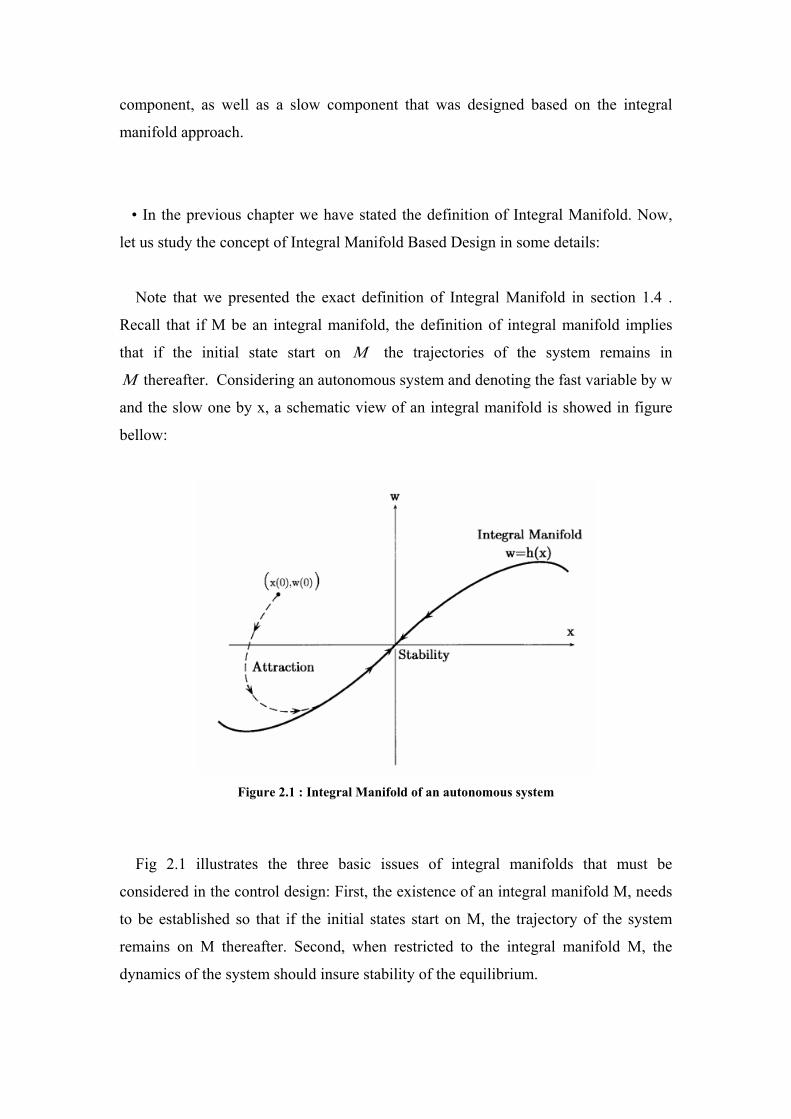
• In the previous chapter we have stated the definition of Integral Manifold. Now,
let us study the concept of Integral Manifold Based Design in some details:
Note that we presented the exact definition of Integral Manifold in section 1.4 .
Recall that if M be an integral manifold, the definition of integral manifold implies
that if the initial state start on Μ the trajectories of the system remains in
thereafter. Considering an autonomous system and denoting the fast variable by w
and the slow one by x, a schematic view of an integral manifold is showed in figure
bellow:
Μ
Figure 2.1 : Integral Manifold of an autonomous system
Fig 2.1 illustrates the three basic issues of integral manifolds that must be
considered in the control design: First, the existence of an integral manifold M, needs
to be established so that if the initial states start on M, the trajectory of the system
remains on M thereafter. Second, when restricted to the integral manifold M, the
dynamics of the system should insure stability of the equilibrium.
Third, the integral manifold M should be attractive so that if the initial conditions
are off M as shown in Fig 2.1, the solution trajectory asymptotically converges to M.
In a control system design context, the challenge is therefore to devise an appropriate
control law u(x, w) that insures the existence of an attractive integral manifold, and
furthermore, insures stability of the system when the dynamics are restricted to the
integral manifold. Note that the fundamental advantage of an integral manifold
approach to control system design is that once an attractive integral manifold is
designed for a dynamical system, the stability problem of the original system reduces
to a stability problem of a lower dimensional system on the manifold which is
typically much easier to deal with.( Note that the fast and the slow manifold for the
singular perturbed system have discussed in the first chapter).
*************************************************
• Robust State and Output Feedback Design :
The problem of designing controllers for nonlinear systems with uncertain variables, is another interesting research subject. In, [27] robust state feedback controllers were synthesized for nonlinear singularly
perturbed systems with time-varying uncertain variables.
[28], studies the problem of synthesizing a robust output feedback controller for
nonlinear singularly perturbed systems with uncertain variables, for which the fast
subsystem is asymptotically stable and the slow subsystem is input/output linearizable
and possesses input-to-state stable inverse dynamics. A dynamic controller is
synthesized, through combination of a high-gain observer with a robust state feedback
controller synthesized via Lyapunov's direct method that ensures boundedness of the
state and achieves asymptotic attenuation of the effect of the uncertain variables on
the output of the closed-loop system. The derived controller enforces the requested
objectives in the closed-loop system, for initial conditions, as long as the singular
perturbation parameter is sufficiently small and the observer gain is sufficiently large.
*************************************************
• Sliding Surface Design :
In [29], Sliding Surface Design for Singularly Perturbed Systems is discussed
and a composite control method through variable structure control design has been
proposed.
In this regard, let us have some discussion about the relationship between the
equilibrium manifold of a singularly perturbed to the sliding surface and also similar
behaviour of fast time and slow time responses to the “reaching mode” and “sliding
mode”:
As we discussed in first chapter the two-time-scale behaviour of a singularly
perturbed system is characterized by a slow and a fast motion in the system dynamics.
The slow motion, approximated by a reduced model, is usually related to a variable
structure system as “sliding mode”. The fast transients, represented by a “boundary
layer” correspond to the “reaching mode” before the state trajectory lies on the sliding
surface. (to have some sense about these similarity, our discussion about fast and slow
manifolds which was given in the first chapter is quite useful).
The composite control method (composition of fast and slow modes control) has a
strong correlation with sliding surface design in that it seeks to determine an
appropriate equilibrium manifold for the slow system to "stay" in. Although this
manifold has an equivalent meaning to a sliding surface, there exist two important
distinctions: First, the dimension of the equilibrium manifold is equal to the number
of fast state variables; while that of a sliding surface is equal to the number of control
variables. Secondly, the way to drive the system into the equilibrium manifold is by

properly designing the fast control part law, which renders an asymptotically stable
boundary layer; while in variable structure design the sliding mode is attained directly
by m ( number of control variables ) discontinuous controls. Lyapunov's approach can
treated as a bridge to soften these differences; that is, to create a sliding motion that
shares the same Lyapunov function as the feedback singularly perturbed system.
2.3 Applications:
Recently, much effort has focused on the stability criteria and control design of
singularly perturbed systems. This is due not only to theoretical interests but also to
the relevance of this topic in control engineering applications. Typical singularly
perturbed systems include direct-drive robots, flexible joint robots, flexible space
structures, armatured-controlled DC motors, high-gain control systems (recall
example 1.2 in first chapter), flexible mechanical systems, tunnel diode circuits,
control system of an airplane, control system of an inverted pendulum, and
nonlinear time-invariant RLC networks.
As we discussed in section 2.2.2 , in [26] the integral manifold design method is
studied. The results are applied to the control problem of multi-body systems with
rigid links and flexible joints in which the inverse of joint stiffness plays the role of
the small parameter.
The proposed composite controller in [26] has the following properties:
(i) It enables the exact characterization and computation of an integral
manifold
(ii) It makes the manifold exponentially attractive
(iii) It forces the dynamics of the reduced flexible system on the integral
manifold to coincide with the dynamics of the corresponding rigid system
(i.e. the one obtained by making stiffness very large) implying that any
control law that stabilizes the rigid system would stabilize the dynamics of
the flexible system on the manifold.
• In [30] the proposed control (geometry approach) has been applied to the
nonlinear automobile idle-speed control system.
The parameterized co-ordinate transformation to transform the original nonlinear
system into singularly perturbed model and the composite Lyapunov approach is then
applied for output tracking.
• In [31] the singular perturbation approach is used to study the diagnosability of
linear two-time scale systems. Based on a power series expansion of the slow
manifold around 0=ε , higher order corrected models for both slow and fast
subsystems are obtained. It is shown that if the original singularly perturbed system is
fault diagnosable, a composite observer-based residual generator for the original
system with actuator faults can be synthesized from the observers of the two separate
subsystems.
• The economic dynamics of reservoir sedimentation management using the hydro
suction-dredging sediment-removal system is analyzed in [32]. In this ariticle, system
dynamics depend on two interdependent hydraulic processes evolving at different
rates. The accumulation of water impounded in the reservoir evolves on a ‘fast’ time
scale, while the loss of water storage capacity to trapped sediments evolves on a
‘slow’ time scale. A multidimensional optimal control problem with singularly
perturbed equations of motion is formulated. Singular perturbation method is applied
to approximate a ‘slow’ manifold and reduce multi-dimensional solution space to the
single-dimensional subspace confining long-term dynamics.
• For the application of singular perturbation in chemical processes, in [33] a
singularly perturbed system of second-order differential equations is considered. This
system describes the steady state of a chemical process that involves three species,
two reactions (one of which is fast), and diffusion.
CHAPTER 3:
Case Study
• Consider the following nonlinear singular perturbed system:
[ ] [ ] 0
2
)0(z)t1(zzx)t1(zz
1)0(xz
)t1(xx
ηε =+−++−=
=+
=
•
•
)2.3(
)1.3(
This system is a bit more complicated that what we have studied in the first chapter,
in a way that setting 0=ε in (3.2), we obtain three isolated roots.
These three roots are :
0z:)3(x)t1(z:)2(
x)t1(z:)1(
=+=+−=
The corresponding boundary layer model to the first root according to (1.7) is given
by:
[ ][ ] )3.3()t1(x)t1(yx)t1(yyddy
+−+−+−−=τ
Using a Lyapunov candidate : 2y21V = ,
[ ][ )t1(x)t1(yx)t1(yyyyyv 2 +−+−+−−==∂∂ •
]
⇓
[ ] [ ] )t1(x)t1(yyx)t1(yyyv 222 ++−++−−=∂∂
In order to having a stable boundary layer model, the function yV∂∂ , must be
negative definite. It is seen that the first term in above equation is negative definite.
To make the second term also negative definite, the condition : must
hold. (due to the existence of coefficient this constraints satisfy the condition
x)t1(y +<
2y
2ycyV
−<∂∂ ).
Assuming x)t1(y +< , the corresponding reduced model for the first root is
obtained as:
)4.3(1)0(xxx =−=•
For the second root the corresponding boundary layer model using (1.7) is given
by:
[ ][ ] )5.3()t1(x)t1(yx)t1(yyddy
++++++−=τ
Using again the Lyapunov candidate : 2y21V = , we have:
[ ][ )t1(x)t1(y)t1(yyyyyv 2 ++++++−==∂∂ •
]
Similar to what we mentioned regard to the first root, here the constraint
must be hold for the stability of the boundary layer model(3.5). x)t1(y +−>
Assuming this constraint is satisfied, we have the following reduced model:
)6.3(1)0(xxx 2 ==•
• Note that (3.6) has a solution )t1(
1x−
= , therefore the simulation time must be
sufficiently smaller than the escape time in 1 sec.
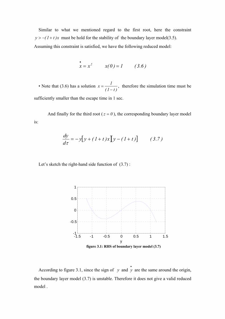
And finally for the third root ( 0z = ), the corresponding boundary layer model
is:
[ ][ ] )7.3()t1(yx)t1(yyddy
+−++−=τ
Let’s sketch the right-hand side function of (3.7) :
-1.5 -1 -0.5 0 0.5 1 1.5-1
-0.5
0
0.5
1
y figure 3.1: RHS of boundary layer model (3.7)
According to figure 3.1, since the sign of and are the same around the origin,
the boundary layer model (3.7) is unstable. Therefore it does not give a valid reduced
model .
y•
y
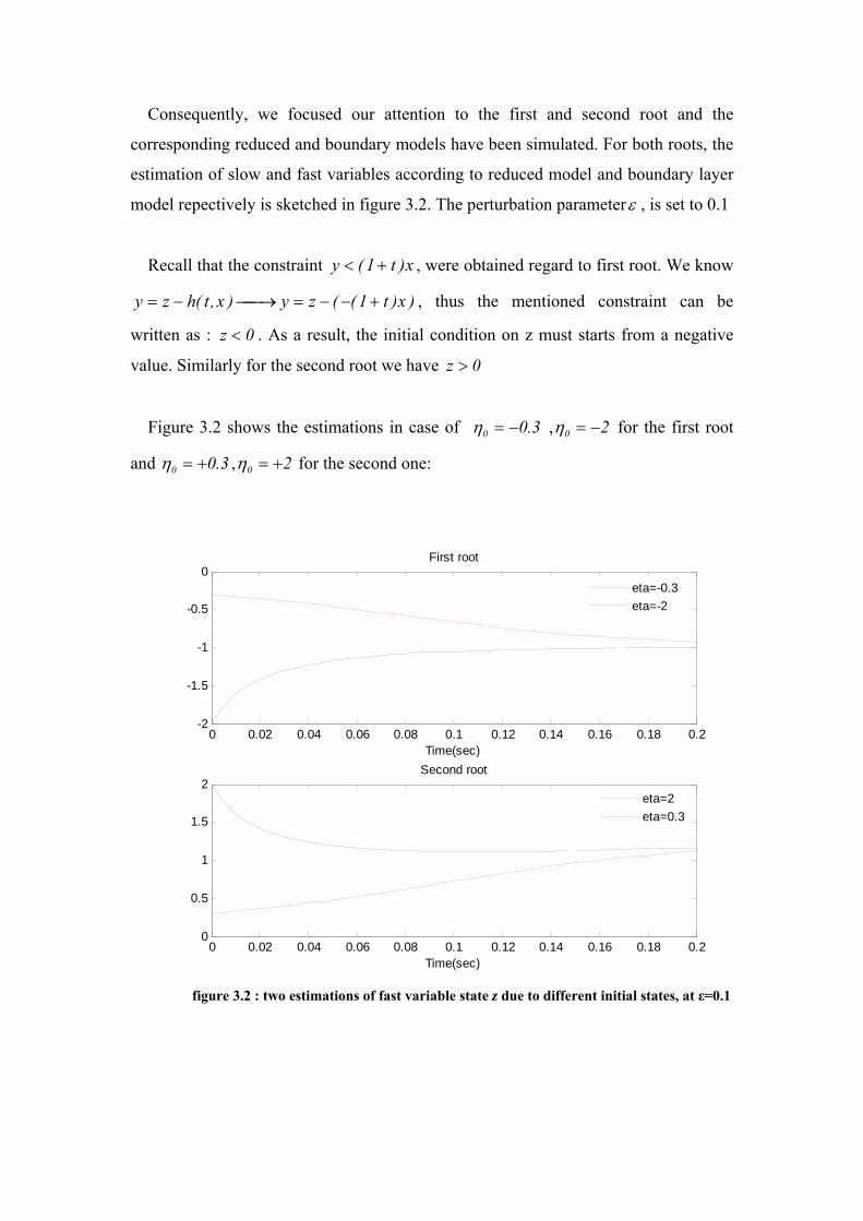
Consequently, we focused our attention to the first and second root and the
corresponding reduced and boundary models have been simulated. For both roots, the
estimation of slow and fast variables according to reduced model and boundary layer
model repectively is sketched in figure 3.2. The perturbation parameterε , is set to 0.1
Recall that the constraint x)t1(y +< , were obtained regard to first root. We know
, thus the mentioned constraint can be
written as : . As a result, the initial condition on z must starts from a negative
value. Similarly for the second root we have
)x)t1((zy)x,t(hzy +−−=⎯→⎯−=
0z <
0z >
Figure 3.2 shows the estimations in case of 3.00 −=η , 20 −=η for the first root
and 3.00 +=η , 20 +=η for the second one:
0 0.02 0.04 0.06 0.08 0.1 0.12 0.14 0.16 0.18 0.2-2
-1.5
-1
-0.5
0First root
Time(sec)
0 0.02 0.04 0.06 0.08 0.1 0.12 0.14 0.16 0.18 0.20
0.5
1
1.5
2
Time(sec)
Second root
eta=2eta=0.3
eta=-0.3eta=-2
figure 3.2 : two estimations of fast variable state z due to different initial states, at ε=0.1
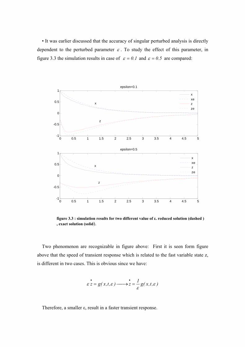
• It was earlier discussed that the accuracy of singular perturbed analysis is directly
dependent to the perturbed parameter ε . To study the effect of this parameter, in
figure 3.3 the simulation results in case of 1.0=ε and 5.0=ε are compared:
0 0.5 1 1.5 2 2.5 3 3.5 4 4.5 5-1
-0.5
0
0.5
1epsilon=0.1
0 0.5 1 1.5 2 2.5 3 3.5 4 4.5 5-1
-0.5
0
0.5
1epsilon=0.5
xxezze
xxezze
x
z
x
z
figure 3.3 : simulation results for two different value of ε. reduced solution (dashed ) , exact solution (solid).
Two phenomenon are recognizable in figure above: First it is seen form figure
above that the speed of transient response which is related to the fast variable state z,
is different in two cases. This is obvious since we have:
),t,x(g1z),t,x(gz εε
εε =⎯→⎯=••
Therefore, a smaller ε, result in a faster transient response.
Second, the figure 3.3 shows that state variables converges to their exact value
faster in case of 1.0=ε . Also the estimation error in this case is fairly lower than the
other case ( 5.0=ε ). This fact can be illustrated as when the value of ε is smaller, as
we said the rate of fast state response is higher, though we can say that when ε, accept
a smaller value, the fast and slow variables are more decoupled. So, the estimation
error is decreased and the convergence rate increases. Lets say the mentioned reason
in another way: recall that the boundary layer model was achieved by setting ε to
zero; so, the boundary layer model and the corresponding reduced model are achieved
on the assumption of ε to be sufficiently close to zero. Therefore, it is logic that
increasing the value of ε, will cause some imperfections.
Conclusion:
We have found the singular perturbed theory a powerful tool for design and
analysis for systems show multiple-time scale behaviour.
We have reviewed important concept and theories involved in singular
perturbation. We found integral manifolds as a useful definition both in analysis and
design of singular perturbed system. In research area chapter, it was seen that the
design methods for the singular perturbed system is completely an open issue. And in
the last chapter we have learned that our estimations are fairly dependent to initial
values and especially to the singular perturbation parameter.
References:
[1] Hassan K. Khalil, Nonlinear systems, Prentice Hall, 2nd edition, (1996).
[2] L.T. Grujic, Uniform asymptotic stability of nonlinear singularly perturbed and large
scale systems, Int. J. Conrr., vol. 33, no. 3., pp 481-504, (1981).
[3] J. H. Chow. Asymptotic stability of a class of nonlinear singularly perturbed systems,
J. Franklin Inst. vol. 305, no. 5, pp. 275-28i, (1978).
[4] A. Saberi, H. Khalil, “Quadratic-Type Lyapunov Functions for Singularly Perturbed
Systems”, IEEE Transaction on Automatic Control, VOL. AC-29, NO. 6, June (1984).
[5] Z.H. Shao and J.R. Rowland, “The Stability Bounds of Linear Time-Delay Singularly
Perturbed Systems”, Proceeding of the American Control Conference, Baltimore, Maryland,
June (1994)
[6] Luse, D. W. “Multivariable singularly perturbed feedback systems with time delay”,
IEEE Transactions on Automatic Control, (1987).
[7] Pan, S.-T., Hsiao, F.-H., & Teng, C. “Stability bound of multiple time delay
singularly perturbed systems”, Electronic Letters, 32, (1996).
[8] Li, X., & de Souza, C. “Criteria for robust stability and stabilization of uncertain
linear systems with state delay”, Automatica, 33, 1657–1662. , (1997).
[9] E. Fridman, “Effects of small delays on stability of singularly perturbed systems.”,
Automatica, 38, 897 – 902, (2002).
[10] M.-C Tsai, “Robust analysis of singularly perturbed system”, Proceeding of the 30th
Conference on Decision and Control, Brighton, England, December (1991).
[11] H. Kwakernaak, & R. Sivan, “Linear optimal control systems”, New York: Wiley,
(1972)
[12] J. H. Chow & P. V. Kokotovic, “Decomposition of near-optimum regulators for
systems with slow and fast modes”, IEEE Transactions on Automatic Control, AC-21, 701–
705, (1976)
[13] Z. GajiAc. & M.-T. Lim, “Optimal control of singularly perturbed linear systems and
applications: High accuracy techniques.“, New York, Marcel Dekker, (2001)
[14] H. D. Tuan and S. Hosoe, “A new design method for regulator problems for
singularly perturbed systems with constrained control”, IEEE Transaction on Automatic
Control, vol. 42, No. 2, February (1997).
[15] H. K. Khalil, “Feedback control of non-standard perturbed systems”, IEEE
Transaction on Automatic Control, vol. 34, No. 10, October (1997).
[16] T.-H S. Lit, M-S. Wang, and Y. Sun, “Dynamic output feedback design for singularly
perturbed discrete systems.”, IMA Journal of Mathematical Control & Information 13. 105-
115
, (1996).
[17] H. K. Khalil, and F. Chen. “H∞ control of two-time-scale systems.”, Systems Control
lett., 19, 35 42, (1992).
[18] H. Oloomi, and M. E. Sawan, “An algorithm for computing the two frequency scale
model matching compensatory”, Proc. ACC. 1640-1641, (1992).
[19] Pan, Z. G. and T. Basar, “H∞ optimal control for singularly perturbed systems”,
Automatica, 29, 401-423, (1993).
[20 W. TAN, T. LEUNGS and Q. TU, “H, Control for Singularly Perturbed Systems”,
Automatica, Vol. 34, No. 2, pp. 255-260, (1998).
[21] E. Fridman, “Robust Sampled-Data Control of Linear Singularly Perturbed Systems”,
Proceedings of the
44th IEEE Conference on Decision and Control, December (2005).
[22] K. V. Zadiraka, “On the integral manifold of a system of differential equations
containing small parameters”, (1957).
[23] K.V. Zadiraka, “On a nonlocal integral manifold of a non-regularly perturbed
differential system.”, (1965).
[24] H.W. Knobloch, B. Aulback, “Singular perturbations and integral manifolds”, J.
Math. Phys. Sci. 18 (5) (1984).
[25] H.W. Knobloch, “Invariant manifolds for ordinary differential equations”, in: C.
Bennewitz (Ed.), Differential Equations and
Mathematical Physics, Mathematics in Science and Engineering, vol. 186, Academic Press,
New York, (1992).
[26] F. Ghorbel, M. W. Spong, “Integral manifolds of singularly perturbed systems with
application to rigid-link flexible-joint multibody systems.”, International Journal of Non-
Linear Mechanics 35 133}155, (2000).
[27] P. D. Christofides, A. R. Teel, and P. Daoutidis,. “Robust semi-global output tracking
for nonlinear singularly perturbed systems.”, International Journal of Control, 65, 639-666,
(1996).
[28] P. D. Christofides “Robust output feedback control of nonlinear singularly perturbed
systems”, Automatica 36 45-52, (2000).
[29] W. C. Su, “Sliding surface design for singularly perturbed systems”, Proceedings of
the American Control Conference, Philadelphia, Pennsylvania, June (1998).
[30] T.-Li. Chiena, C.-C. Chenb and C-Y. Hsu, “Tracking control of nonlinear automobile
idle-speed time-delay system via differential geometry approach.”, Journal of the Franklin
Institute 342 760–775, (2005).
[31] F. Gong and K. Khorasani, “Fault Diagnosis of linear singularly perturbed systems”,
Proceedings of the 44th IEEE Conference on Decision and Control, December (2005).
[32] R. Huffakera, R. Hotchkissb, “Economic dynamics of reservoir sedimentation
management: Optimal control with singularly perturbed equations of motion.”, Journal of
Economic Dynamics & Control 30 2553–2575, (2006).
[33] L. V. Kalachev and T. I. Seidman, “Singular perturbation analysis of a stationary
diffusion/reaction system whose solution exhibits a corner-type behavior in the interior of the
domain”, J. Math. Anal. Appl. 288 722–743, (2003).