January 2008

Oklahoma Councilof Public Affairs

2

Executive Summary

Oklahoma imposes a relatively low taxburden: total state and local tax revenues are9.0% of total state personal income. Nation-ally, the average state and local tax revenuesare 11.0% of total state personal income. Verylow property tax burdens are an importantreason Oklahoma’s overall tax burden is solow.

Not surprisingly, Oklahoma’s relativeeconomic growth compares very favorably tothe nation’s. Per capita personal income in2006 grew by 7.8% in Oklahoma compared to5.6% for the nation as a whole.

While Oklahoma’s relatively low state andlocal tax burden provides a competitiveadvantage for the state, there are someconcerns. Oklahoma’s marginal tax rates onpersonal income, corporate income, andcapital gains are relatively high—especiallycompared to those of neighboring Texas andColorado. High marginal tax rates on incomeand capital gains diminish economic incen-tives to produce, save, and invest in Okla-homa. On the spending side, the recentacceleration in expenditures is also troubling,as the higher expenditures, if not curtailed,will negatively impact Oklahoma’s positiveeconomic growth environment.

Oklahoma’s experience since the 1970sillustrates the importance of establishing astrong pro-growth tax environment. Histori-cally, when Oklahoma’s state and local taxburden was rising compared to the nationalaverage, economic growth in the state laggedoverall national economic growth. The reversehas occurred when Oklahoma’s state andlocal tax burden was declining relative to thenational average. This real-world experienceis precisely what the theory of pro-growth taxpolicies predicts.

Based on the theory of pro-growth taxpolicy, OCPA reviewed Oklahoma’s tax sys-tem. Our analysis indicates that, while overallOklahoma’s tax system is good, there areseveral key areas for improvement, especiallyin comparison to neighboring Texas andColorado. Specifically:• Oklahoma’s low overall state and local tax

burden and low property tax burden areimportant competitive advantages for thestate, which should be maintained.

• Oklahoma’s top marginal personal incomeand corporate income tax rates are toohigh—especially compared to neighboringTexas and Colorado. Tax reforms shouldlower these top marginal tax rates to bringthem closer in line with neighboring Texasand Colorado.

• Oklahoma’s personal income tax has seventax brackets, which is progressive. In gen-eral, progressive tax structures add signifi-cant complexity to the tax code, while thehigher top marginal income tax rates tendto diminish pro-growth incentives through-out the economy. In Oklahoma, the topmarginal personal income tax rate becomeseffective at $8,700 for a single filer, which isless than the annual salary for a full-timeminimum wage worker. The low incomethreshold for the top marginal income tax inOklahoma creates an additional argumentfor eliminating the progressive income taxstructure in Oklahoma and replacing thecomplex structure with a simpler flat-ratetax.

• Oklahoma imposes a relatively high capitalgains tax rate. This rate should be reducedand, at a bare minimum, brought into linewith the capital gains taxes that are im-posed in neighboring states.

• While Oklahoma’s spending record hastraditionally been competitive from a na-tional perspective, overall spending hasbeen growing at a troubling pace as of late.Furthermore, spending per capita in thestate has been above several key neigh-bors, including Texas and Colorado. Inorder to enhance the effectiveness of thepro-growth tax reforms suggested above,the per capita spending of state and localgovernments should be brought into linewith Texas and Colorado.Ideas for restraining spending in Oklahoma

are not wanting. For instance, OCPA annuallypresents detailed spending budgets whichlimit government growth.

3

Oklahoma’s tax and spending policies have alarge and significant impact on the state’s overalleconomic performance. When Oklahoma’s stateand local tax burden is increasing, Oklahoma’seconomic performance is less than the nationalaverage. Conversely, when Oklahoma’s state andlocal tax burden is decreasing, Oklahoma’s eco-nomic performance exceeds the national average.

On the surface, the trade-off between low taxesand economic growth appears to imply a trade-offbetween economic growth and adequate rev-enues for the state and local governments. Inreality, the reverse is true. The optimal tax systemfor Oklahoma ensures adequate and stablerevenues for state and local governments over thelong term while simulta-neously ensuring strongeconomic growth for the stateand its citizens. This paperwill discuss the importance ofestablishing pro-growth fiscalpolicies and illustrate thatimplementing pro-growth taxreforms with sound budgetpractices will maintain thestrong economic performance as of late, whilemaximizing Oklahoma’s long-run economicgrowth potential and providing a solid and stablerevenue source for state and local governments.

Before we apply the lessons of past fiscalpolicies to Oklahoma, it is useful to review thehistory and theory of pro-growth tax policies. Thefirst half of this paper reviews the theories andlessons from past tax policy changes. With thisbackground, the second half of this paper reviewsOklahoma’s tax and spending history, applyingthe lessons of the past to Oklahoma’s future.The Theory Behind Low, Broad-Based Taxes

Excessive taxation is detrimental to labor andcapital, poor and rich, men and women, and oldand young. Excessive taxation is an equal oppor-tunity tormentor. In the short run, higher taxes onlabor or capital lower after-tax earnings. In thelonger run, mobile factors “vote with their feet”and leave the state, while immobile factors (suchas low-wage workers and land and property) areleft to suffer the tax burden. The principals ofArduin, Laffer & Moore Econometrics have pro-duced decades of research demonstrating thatstates where taxes are high and/or increasingrelative to the national norm experience decliningrelative income growth, declining relative popula-

tion growth, rising relative unemployment, anddeclining housing values.

The mode of taxation is as important as theamount of taxation, as noted by 19th centuryAmerican economist Henry George:

The mode of taxation is, in fact, quite asimportant as the amount. As a small burdenbadly placed may distress a horse that couldcarry with ease a much larger one properlyadjusted, so a people may be impoverishedand their power of producing wealth destroyedby taxation, which, if levied in any other way,could be borne with ease.1

While the world is dynamic and many of its upsand downs are outside the control of state govern-

ment, there are a number ofcriteria for judging theefficacy of a state’s taxsystem. These were summa-rized well by Henry George:

The best tax by whichpublic revenues can beraised is evidently thatwhich will closest conformto the following conditions:

1. That it bear as lightly as possible uponproduction—so as least to check the increaseof the general fund from which taxes must bepaid and the community maintained.2. That it be easily and cheaply collected, andfall as directly as may be upon the ultimatepayers—so as to take from the people as littleas possible in addition to what it yields thegovernment.3. That it be certain—so as to give the leastopportunity for tyranny or corruption on thepart of officials, and the least temptation tolawbreaking and evasion on the part of thetaxpayers.4. That it bear equally—so as to give nocitizen an advantage or put any at a disad-vantage, as compared with others.2

The theory of incentives provides the basis forestablishing an optimal tax policy. Incentives canbe either positive or negative. They are alternatelydescribed as carrots and sticks or pleasure andpain. Whatever their form, people seek positiveincentives and avoid negative incentives. Theprinciple is simple enough: If an activity should beshunned, a negative incentive is appropriate, andvice versa.

In the realm of economics, taxes are negative

High marginal tax rates on

income and capital gains

diminish economic

incentives to produce, save,

and invest in Oklahoma.

4

incentives, and government subsidies are positiveincentives, subject to all the subtleties and intrica-cies of the general theory of incentives. Peopleattempt to avoid taxed activities—the higher thetax, the greater their attempt to avoid. As with allnegative incentives, no one can be sure how theavoidance will be carried out.

Changes to marginal tax rates are critical forgrowth because they change incentives to de-mand, and to supply work effort and capital.Firms base their decisions to employ workers, inpart, on the workers’ total cost to the firm. Holdingall else equal, the greater the cost to the firm ofemploying each additional worker, the fewerworkers the firm will employ. Conversely, the lowerthe marginal cost per worker, the more workersthe firm will hire. For the firm, the decision toemploy is based upon gross wages paid, a conceptwhich encompasses all costs borne by the firm.

Workers, on the other hand, care little about thecost to the firm of employing them. Of concernfrom a worker’s standpoint is how much the

worker receives for providing work effort, net of alldeductions and taxes. Workers concentrate on netwages received. The greater the net wagesreceived, the more willing a worker is to work. Ifwages received fall, workers find work effort lessattractive and they will do less of it. The differencebetween what it costs a firm to employ a workerand what that worker receives net is the tax wedge.Tax Policy Matters for Economic Growth

Rising tax burdens are detrimental to economicgrowth. States that have high and/or increasingtaxes relative to the national average experiencerelative declines in income, housing values, andpopulation, as well as rising relative unemploy-ment rates.

Consistently, economic growth rates in thestates with the highest tax burdens lag the eco-nomic growth rates in the states with the lowesttax burdens. Table 1 summarizes the latest results.

Economic growth in the 10 states with thelowest tax burden, defined as total state and localtaxes as a percentage of personal income,

Table 1State and Local Tax Burden vs. 10-Year Economic Performance(2006 state and local tax burden vs. economic performance between 1996 and 2006, unless otherwise noted)

Net Domestic Non-Farm 2006 Personal In-Migration Payroll Unemployment S&L Tax Income Population as a % of Employment Rate, Burden Growth Growth Population Growth 2006

South Dakota $87.40 76.0% 5.2% -1.8% 14.5% 3.2% Tennessee $88.99 63.6% 11.9% 4.3% 9.6% 5.2% Alabama $90.44 61.6% 6.1% 0.8% 8.0% 3.5% New Hampshire $90.51 73.0% 13.2% 6.0% 15.9% 3.4% Colorado $94.00 88.5% 21.9% 5.1% 19.5% 4.4% Missouri $98.48 56.6% 7.8% 1.3% 7.3% 4.8% Texas $99.49 87.2% 20.6% 2.1% 20.8% 5.0% Oklahoma $100.21 70.1% 7.2% 0.1% 13.8% 3.9% Oregon $101.10 65.0% 14.3% 4.7% 16.0% 5.4% Georgia $102.50 78.1% 23.8% 6.4% 15.7% 4.7%

10 States WithLowest Tax Burden $95.31 72.0% 13.2% 2.9% 14.1% 4.4%

10 States With Highest Tax Burden $132.31 59.5% 5.5% -2.3% 12.9% 4.4%Connecticut $119.41 61.6% 5.6% -3.1% 5.6% 4.3% Wisconsin $121.73 59.8% 6.8% 0.6% 10.3% 4.7% West Virginia $123.38 46.3% -0.4% -0.5% 8.2% 4.8% Rhode Island $125.32 60.5% 5.8% -1.9% 11.8% 5.3% Alaska $131.39 52.6% 9.8% -3.9% 19.4% 6.8% Hawaii $133.05 46.9% 6.5% -6.5% 16.5% 2.6% Maine $134.56 62.6% 6.3% 3.7% 13.1% 4.6% Wyoming $140.43 86.0% 5.0% -2.0% 23.9% 3.2% Vermont $143.29 64.9% 5.8% 1.0% 11.9% 3.5% New York $150.52 53.8% 3.9% -10.1% 8.3% 4.5%

Sources: U.S. Bureau of Economic Analysis, U.S. Census, U.S. Bureau of Labor Statistics, and ALME calculations

5

exceeds the economic growth in the 10 states withthe highest tax burdens. Overall economic growth,as measured by total economic activity (stateGDP) or residents’ total personal income, hasbeen significantly higher in the low-tax states.

Not surprisingly, stronger economic growth hasled to more jobs and lower unemployment rates—this despite the higher population growth in thelow-tax states, as more and more people chooseto relocate to the lower-taxed states. Similar to theexperience of the low-tax states, economic growthin the states with no personal income tax exceedseconomic growth in the states with the highestpersonal income tax burdens. Table 2 illustratesthis relationship.

Further substantiating the relationship betweenpersonal income taxes and economic growth, weexamined the top marginal state and local per-sonal income tax rates and compared them toeach state’s overall economic growth for 2006.While there is some dispersion in the results, duein part to other factors that will impact state

economic growth, there is a definite negativerelationship between a state’s top marginalpersonal income tax rate and the economicgrowth rate in the state—the higher the top mar-ginal personal income tax rate, the lower theexpected economic growth rate.3 This relationshipis not unique to 2006 either. Since 1999, the stateswith higher marginal income tax rates tend tohave slower state personal income growth, exceptfor the recession year of 2001.Voting With Their Feet: A Hypothetical Example

Each state in the U.S. is analogous to a countrywith open borders. Just as the U.S. competes withother countries for the location of economicactivity, states compete with each other for thelocation of factories, offices, and jobs within theU.S. This competition is seen through tax-cuttingbattles between neighboring states and targetedtax incentives to encourage corporate relocation.As states seek to hold companies and workerswithin their borders and attract new ones, thewinners and the losers will be separated by their

Table 2Relationship between 2006 State Personal Income Growthand Top Marginal Personal Income Tax Rate (State and Local) Personal Net Domestic Non-Farm Top GDP Personal Income In-Migration Payroll Unemployment PIT by State Income Per Capita Population as a % of Employment Rate, Rate Growth Growth Growth Growth Population Growth 2006

Alaska 0.00% 70.2% 52.6% 39.6% 9.8% -3.9% 19.4% 6.8%Florida 0.00% 94.0% 83.9% 46.4% 22.4% 8.9% 30.4% 3.2%Nevada 0.00% 123.7% 120.1% 44.6% 52.7% 20.5% 52.9% 4.1%New Hampshire 0.00% 73.9% 73.0% 55.2% 13.2% 6.0% 15.9% 3.4%South Dakota 0.00% 71.0% 76.0% 62.1% 5.2% -1.8% 14.5% 3.2%Tennessee 0.00% 66.3% 63.6% 46.9% 11.9% 4.3% 9.6% 5.2%Texas 0.00% 96.9% 87.2% 54.6% 20.6% 2.1% 20.8% 5.0%Washington 0.00% 72.7% 70.6% 49.5% 14.7% 3.1% 18.6% 5.0%Wyoming 0.00% 101.5% 86.0% 74.8% 5.0% -2.0% 23.9% 3.2%9 States WithNo PIT 0.00% 85.6% 79.2% 52.6% 17.3% 4.1% 22.9% 4.3%9 StatesWith HighestMarginal PIT Rate 9.12% 62.1% 59.6% 49.5% 7.6% -1.8% 12.1% 4.6%Kentucky 8.20% 49.6% 61.0% 51.0% 7.4% 1.7% 10.4% 5.8%Hawaii 8.25% 49.2% 46.9% 38.1% 6.5% -6.5% 16.5% 2.6%Maine 8.50% 57.8% 62.6% 55.2% 6.3% 3.7% 13.1% 4.6%Ohio 8.87% 47.3% 45.0% 44.4% 2.3% -2.8% 3.0% 5.4%New Jersey 8.97% 59.1% 63.3% 51.2% 7.9% -4.2% 12.1% 4.8%Oregon 9.00% 81.8% 65.0% 44.0% 14.3% 4.7% 16.0% 5.4%Vermont 9.50% 69.2% 64.9% 58.7% 5.8% 1.0% 11.9% 3.5%California 10.30% 80.1% 74.1% 53.3% 14.0% -3.5% 17.7% 4.8%New York 10.50% 64.4% 53.8% 49.6% 3.9% -10.1% 8.3% 4.5%

Sources: U.S. Bureau of Economic Analysis, U.S. Census, U.S. Bureau of Labor Statistics, and ALME calculations

6

ability to understand the competitive environmentin which they exist and take steps to enhance theirown state’s appeal. Since monetary policy andfederal fiscal policy are basically the same for allof the states, and inherent state advantages anddisadvantages (such as climate, natural re-sources, distances to desirable areas, etc.) remainfairly constant over time, state and local fiscalpolicies are far and away the most importantfactors determining changes in the competitive-ness and, hence, relative economic growth ratesamong the states.

The overall level of taxation in a state is alsocritical. Overtaxed states per se restrain growth,while states—even if they currently aren’t over-taxed—that raise taxes inhibit growth. A reductionin tax rates reduces the cost of doing business ina state. This increasesdemand for the now less-expensive goods and ser-vices produced within thestate. The higher demand forthe state’s goods and ser-vices will result in an in-creased profitability forbusinesses located within thestate. Business failures willdecrease in states withdeclining relative tax burdens, and businessstarts will rise. If all else remains the same, areduction in tax rates increases the return tocapital and work effort, leading to increases in thesupplies of capital and labor within the state.

Symmetrically, every state that raises its rela-tive tax burden will find it difficult to retain exist-ing facilities and attract new businesses andworkers. In tax-raising states, new business startswill decline, and business failures will increase.

Competition among the many states results, inlarge part, from the ability of mobile factors ofproduction to “vote with their feet” and relocate topolitical jurisdictions pursuing more favorableeconomic policies. Changes in tax rates have thegreatest impact on the supplies of factors ofproduction that are highly mobile. For example, aworker who is prepared to relocate to achieve ahigher standard of living will be extremely sensi-tive to a change in his state’s tax rates. By con-trast, the supplies of immobile factors of produc-tion and/or real estate will be affected onlyslightly by tax rate changes. For example, capitalin the form of a new manufacturing plant, as in

the case of the example below, is highly immobile.Its operating level initially will be relatively unaf-fected by an increase in a state’s tax rates. Themajor impact of state tax rate changes will be onthe plant’s after-tax profits and, ultimately,whether to close down or to remain open. Theimplication of this analysis is that taxes levied onmobile factors will be passed on to the immobilefactors located within the state. Thus, the burdenof state and local taxes may very well be differentfrom its initial incidence.

Consider two hypothetical manufacturingcompanies with production plants located withinjust miles of each other. One is located in Okla-homa, and the other, virtually identical to the first,is located just across the border in Texas. Sincewe assume both companies sell virtually identical

products in the U.S. market,competition will force themto sell their products atapproximately the sameprice. Because eachcompany’s plant is sepa-rated by just a thin andinvisible state line, bothhave to pay the same inter-est cost on borrowings, thesame after-tax wages to

their employees, and the same prices to theirsuppliers.

Now, consider what would happen if Oklahomawere to put through a large corporate income taxincrease, while Texas held constant or lowered itscorporate income tax rate. Because the market forthe companies’ product is highly competitive, theOklahoma company would not be able to passthe tax hike forward to its customers in the form ofhigher prices. Likewise, the Oklahoma companywould not be able to pass the tax hike backwardonto its suppliers or employees. The Oklahomafirm would have to absorb the tax increasethrough lower after-tax profits. This drop in profitswould be reflected by a fall in the Oklahomacompany’s stock price. Clearly, the identicalcompetitor in Texas would benefit.

Whether the price of a commodity or factor ofproduction is equilibrated across states on apretax or after-tax basis depends on each item’smobility. This means that changes in tax rates willhave two general effects. First, they will changethe quantity and pretax price of mobile factorswithin the state and leave their after-tax rates of

President Kennedy

understood that tax

reduction ‘sets off a process

that can bring gains for

everyone, gains won by

marshalling resources that

would otherwise stand idle.’

7

return unchanged. Second, they will change therate of return of factors of production that cannotleave the state and leave the quantity within thestate unchanged.

As time horizons lengthen following tax in-creases or tax cuts, the process of adjustment willincorporate the movement of capital and laborinto or out of the state. This migration of factors ofproduction will continue until after-tax returns formobile factors within the state are equalized withafter-tax returns for their counterparts elsewherein the economy. The returns of state-specificimmobile factors will reap the benefit or bear theburden of the result of the tax change.The Dynamic Effects of Lower Marginal

Tax Rates

It is always difficult to project the dynamiceffects of supply-side policy changes. Estimatingwhat will happen as a consequence of a taxincrease or tax cut is precarious to say the least.But failing to estimate the dynamic consequencesof tax changes will always be wrong. With incred-ible clarity, none other than John Maynard Keynesdescribed these difficulties:

When, on the contrary, I show, a little elabo-rately, as in the ensuing chapter, that to createwealth will increase the national income andthat a large proportion of any increase in thenational income will accrue to an Exchequer,amongst whose largest outgoings is the pay-ment of incomes to those who are unemployedand whose receipts are a proportion of theincomes of those who are occupied, I hope thereader will feel, whether or not he thinks himselfcompetent to criticize the argument in detail,that the answer is just what he would expect—that it agrees with the instinctive promptings ofhis common sense.

Nor should the argument seem strange thattaxation may be so high as to defeat its object,and that, given sufficient time to gather thefruits, a reduction of taxation will run a betterchance than an increase of balancing thebudget. For to take the opposite view today is toresemble a manufacturer who, running at aloss, decides to raise his price, and when hisdeclining sales increase the loss, wrappinghimself in the rectitude of plain arithmetic,decides that prudence requires him to raise theprice still more—and who, when at last hisaccount is balanced with nought on both sides,is still found righteously declaring that it would

have been the act of a gambler to reduce theprice when you were already making a loss.4

There are several major tax changes that haveoccurred at the state and federal levels. Each oneof these case studies illustrates the positiveeconomic impact pro-growth tax reform can have.California’s Proposition 13

In 1978, a force that had been building strengthfor several years finally brought a huge anddramatic change to the California economy. Thepublic’s frustration with high and rising state andlocal (particularly property) taxes found expres-sion in the passage of Proposition 13—an initia-tive to limit state and local spending and taxation.In June 1978, Proposition 13 roiled the entrenchedpolitical establishment. Proposition 13 was a stateconstitutional amendment that (1) set propertytaxes not to exceed 1% of a property’s value(down from the 3.5% rate that existed at the time),(2) rolled assessed property tax values back totheir 1976 levels, (3) allowed the base value togrow no more than 2% per year unless the prop-erty changed hands, and (4) required that all newor increased taxes be voted in by a supermajorityof the electorate. Proposition 13 won in a landslide.

Following on Proposition 13’s heels was anelimination of the state’s inheritance tax, anindexing of the state’s income tax, and an elimi-nation of the state’s business inventory tax. In1979, Proposition 4 passed, locking the tax gainsinto place by requiring (1) spending to grow nofaster than the sum of population growth andinflation and (2) all surplus revenues to be re-turned to the taxpayers.

Prior to the passage of Proposition 13 in Marchof 1978, Arthur Laffer wrote an economic analysiswhich was used by the United Organization ofTaxpayers, detailing support for the passage ofProp 13.5 This analysis included forecasts of whatthe initiative’s effects would be, and almost allwere spot on. In the aftermath of this tax revolt thepreviously chronically depressed Californiaenjoyed a remarkable economic resurgence,outperforming the nation in nearly every conceiv-able measure. Naturally, the state’s high taxburden fell like a stone, from $124.57 to $95.19 justone year later.6 In 1977, California per capitapersonal income was 15% above the nationalaverage.7 Three years later, it was 18% above thenational average.8 California’s unemploymentrate was 1.2 percentage points higher than theU.S. rate in 1977; in 1980 the California rate was

lower than the national rate by 0.4 percentagepoints.9 Between 1978 and 1988 the number ofjobs in California increased by 32%, twice the16% increase in jobs nationwide.10 The populationin California increased by 24% from 1978 to 1988,over twice the national increase of 10.7%.11

Housing prices in the state soared. There isperhaps no better barometer for changes in theafter-tax rate of return on assets than the price ofthe ultimate immobile factor: housing. In thesecond quarter of 1978, right before Proposition13’s passage, the median home price in Califor-nia was $70,677, which was 7.4 times per capitapersonal income in the state and 21% moreexpensive relative to the U.S.12 Over the decade ofthe 1980s absolute and relative housing prices inCalifornia took off and never looked back. In thethird quarter of 1981, themedian home price inCalifornia was $108,455, or8.1 times per capita per-sonal income and 42% moreexpensive relative to theU.S. By the end of thedecade, per capita personalincome-adjusted housingprices in California werenearly double those for theU.S.13

Prop 13 did what it was advertised to do. Thehistorical record also shows that Proposition 13did not have any long-term deleterious effect onthe finances of the state’s various levels of govern-ment. The Great California Tax Revolt more thanpaid for itself.

The private sector of the economy fared beauti-fully in the aftermath of Proposition 13, but oppo-nents questioned whether this private sectorsuccess might have come at the expense of thepublic sector. They feared that post-Proposition 13revenues would be absolutely gutted, forcingexpenditure cuts well beyond the elimination ofwasteful spending. Vital services, they said, wouldsuffer; schools would have to close; fire andpolice protection would no longer be adequate.But the fears of citizens concerned about main-taining adequate levels of state and local govern-ment services were allayed very soon after thechanges were enacted.

First looking at revenues, Proposition 13 passedon June 6, 1978, one month prior to the end ofFY1978. State and local property tax revenues fell

$5.0 billion, from $11.0 billion in FY1978 to $6.0billion in FY1979, far short of the static revenueloss forecasts of $7 billion. In addition, this dropwas largely offset by higher revenues in everyother major tax category. Total state and localrevenues fell by only $1.1 billion that first year.14

Looking at the bigger picture, the combinedstate and local tax burden per $1,000 of personalincome fell from $124.57 in FY1978 to $94.93 inFY1982, a 24% reduction.15 Yet, in spite of theprecipitous fall in the state’s average tax rate,state and local revenues did not fall proportion-ately. In fact, total tax revenue grew by 19% from$27.4 billion in FY1978 to $32.5 billion in FY1982.16

The tax base expanded more than enough tooffset the reduction in tax rates. Even after adjust-ing for inflation, which can distort economic data

during this high inflationaryperiod, tax revenues fellmuch less than the reduc-tion in the state and localtax burden.

Economic expansion andhigher property values ledto healthy property taxgrowth over the followingyears, and by FY1985property tax collections were

back to their FY1978 $11.0 billion level.17 Thedisruptive shortage of funds so widely anticipatednever materialized.

Turning our attention to spending, total stateand local direct general expenditures were notslashed between FY1978 and FY1979 as skepticshad predicted; in fact, expenditures increased1.6% from $36.9 billion to $37.5 billion over thisperiod.18 The tax reduction which had invigoratedthe state’s economy so profoundly did not imposeany significant reduction in government services.

The state’s balanced budgets during thisperiod reflect the remarkable success of combin-ing lower tax rates and increased output, employ-ment, and production with restrained spending.California’s experience following Proposition 13exemplifies the types of pro-growth dynamics thatfollow sound tax reform. These effects have beenexperienced at the federal level as well.The Harding/Coolidge Tax Cuts

In 1913, the federal progressive income tax wasput into place with a top marginal rate of 7%.Thanks in part to World War I, this tax rate wasquickly increased significantly and peaked at

8

The real-world experiences of

California’s Prop 13—as well

as the Harding/Coolidge,

Kennedy, and Reagan tax

cuts/reforms—illustrate the

power of reducing marginal

income tax rates.

77% in 1918. Then, through a series of tax-ratereductions, the Harding/Coolidge tax cutsdropped the top personal marginal income taxrate to 25% in 1925.

While tax collection data for the NationalIncome and Product Accounts (from the U.S.Bureau of Economic Analysis) do not exist for the1920s, we do have total federal receipts from theU.S. budget tables. During the four years prior to1925 (the year the tax cut was fully enacted),inflation-adjusted revenues declined by an aver-age of 9.2% per year. Over the four years follow-ing the tax-rate cuts, revenues remained volatilebut averaged an inflation-adjusted gain of 0.1%per year. The economy responded strongly to thetax cuts, with output nearly doubling and unem-ployment falling sharply.

Perhaps most illustrative of the power of theHarding/Coolidge tax cuts was the increase inGDP, the fall in unemployment, and the improve-ment in the average American’s quality of life overthis decade. Table 3 demonstrates the remarkableincrease in American quality of life, as reflectedby the percentage of Americans owning items in1930 that previously had only been owned by thewealthy (or by no one at all).

Table 3Percentage of Americans Owning Selected ItemsItem 1920 1930

Autos 26% 60%

Radios 0% 46%

Electric lighting 35% 68%

Washing machines 8% 24%

Vacuum cleaners 9% 30%

Flush toilets 20% 51%Source: Stanley Lebergott, Pursuing Happiness: AmericanConsumers in the Twentieth Century (Princeton: PrincetonUniversity Press, 1993), pp. 102, 113, 130, 137.

The Kennedy Tax Cuts

During the Depression and World War II the topmarginal income tax rate rose steadily, peaking atan incredible 94% in 1944 and 1945. The rateremained above 90% well into President John F.Kennedy’s term in office, which began in 1961.Kennedy’s fiscal policy stance made it clear hewas a believer in pro-growth, supply-side taxmeasures. Kennedy said it all in January of 1963in the Economic Report of the President:

Tax reduction thus sets off a process that canbring gains for everyone, gains won by mar-

shalling resources that would otherwise standidle—workers without jobs and farm andfactory capacity without markets. Yet manytaxpayers seemed prepared to deny the nationthe fruits of tax reduction because they questionthe financial soundness of reducing taxes whenthe federal budget is already in deficit. Let memake clear why, in today’s economy, fiscalprudence and responsibility call for tax reduc-tion even if it temporarily enlarged the federaldeficit—why reducing taxes is the best wayopen to us to increase revenues.19

Kennedy further reiterated his beliefs in his TaxMessage to Congress on January 24, 1963:

In short, this tax program will increase ourwealth far more than it increases our publicdebt. The actual burden of that debt—asmeasured in relation to our total output—willdecline. To continue to increase our debt as aresult of inadequate earnings is a sign ofweakness. But to borrow prudently in order toinvest in a tax revision that will greatly increaseour earning power can be a source of strength.20

President Kennedy proposed massive tax-ratereductions which passed Congress and went intolaw after he was assassinated. The 1964 tax cutreduced the top marginal personal income taxrate from 91% to 70% by 1965. The cut reducedlower-bracket rates as well. In the four years priorto the 1965 tax-rate cuts, federal governmentincome tax revenue, adjusted for inflation, hadincreased at an average annual rate of 2.1%,while total government income tax revenue (fed-eral plus state and local) had increased 2.6% peryear.21 In the four years following the tax cut thesetwo measures of revenue growth rose to 8.6% and9.0%, respectively.22 Government income taxrevenue not only increased in the years followingthe tax cut, it increased at a much faster rate inspite of the tax cuts.

The Kennedy tax cut set the example thatRonald Reagan would follow some 17 years later.By increasing incentives to work, produce, andinvest, real GDP growth increased in the yearsfollowing the tax cuts, more people worked, andthe tax base expanded. Additionally, the expendi-ture side of the budget benefited as well becausethe unemployment rate was significantly reduced.

Testifying before Congress in 1977, WalterHeller, President Kennedy’s Chairman of theCouncil of Economic Advisors, summed it all up:

What happened to the tax cut in 1965 is

9

difficult to pin down, but insofar as we are ableto isolate it, it did seem to have a tremendouslystimulative effect, a multiplied effect on theeconomy. It was the major factor that led to ourrunning a $3 billion surplus by the middle of1965 before escalation in Vietnam struck us. Itwas a $12 billion tax cut, which would be about$33 or $34 billion in today’s terms, and withinone year the revenues into the Federal Treasurywere already above what they had been beforethe tax cut.

Did the tax cut pay for itself in increased rev-enues? I think the evidence is very strong that it did.23

The Reagan Tax Cuts

In August of 1981, Ronald Reagan signed intolaw the Economic Recovery Tax Act (ERTA, alsoknown as Kemp-Roth). ERTAslashed marginal earnedincome tax rates by 25%across the board over athree-year period. Thehighest marginal tax rate onunearned income dropped to50% from 70% immediately(the Broadhead Amend-ment), and the tax rate oncapital gains also fell imme-diately from 28% to 20%. Five percentage pointsof the 25% cut went into effect on October 1, 1981.An additional 10 percentage points of the cut thenwent into effect on July 1, 1982, and the final 10percentage points of the cut began on July 1, 1983.

Looking at the cumulative effects of ERTA interms of tax (calendar) years, the tax cut provideda reduction in tax rates of 1.25% through theentirety of 1981, 10% through 1982, 20% through1983, and the full 25% through 1984.

As a provision of ERTA, Reagan also saw to itthat the tax brackets were indexed for inflationbeginning in 1985.

To properly discern the effects of the tax-ratecuts on the economy, we use the starting date ofJanuary 1, 1983, given that the bulk of the cutswere in place on that date. However, a case couldbe made for a start date of January 1, 1984, thedate the full cut was in effect.

These across-the-board marginal tax-rate cutsresulted in higher incentives to work, produce,and invest, and the economy responded. Between1978 and 1982 the economy grew at a 0.9% rate inreal terms, but from 1983 to 1986 this growth rateincreased to 4.8%.24

Prior to the tax cut, the economy was chokingon high inflation, high interest rates, and highunemployment. All three of these economicbellwethers dropped sharply after the tax cuts.The unemployment rate, which had peaked at9.7% in 1982, began a steady decline, reaching7.0% by 1986 and 5.3% when Reagan left office inJanuary 1989.25

Inflation-adjusted revenue growth dramaticallyimproved. Over the four years prior to 1983,federal income tax revenue declined at an aver-age rate of 2.8% per year, and total governmentincome tax revenue declined at an annual rate of2.6%. Between 1983 and 1986 these figures were apositive 2.7% and 3.5%, respectively.26

The most controversial portion of Reagan’s taxrevolution was the big dropin the highest marginalincome tax rate from 70%when he took office to 28%in 1988. However, InternalRevenue Service data revealthat tax collections from thewealthy, as measured bypersonal income taxes paidby top percentile earners,increased between 1980 and

1988 despite significantly lower tax rates.Lessons for Oklahoma’s Tax Policy

The real world experiences of California’sProposition 13 or the Harding/Coolidge, Kennedy,and Reagan tax cuts/reforms at the federal levelillustrate the power of reducing marginal incometax rates. In Oklahoma, reforms to the state taxcode should heed the lessons from the previousmajor tax reforms.

All tax changes create two primary economiceffects. Economists deem these the income effectand the substitution effect. The income effectexamines the changed behavior that directlyarises from changes in income or wealth. Forexample, people will tend to increase the amountof consumption in response to an increase inincome. The substitution effect examines thechanged behavior that arises from changes in therelative costs of different goods or activities. Forexample, a switch in tax policy that reduces thecosts of one good compared to another willprovide incentives for people to consume more ofthe former at the expense of the latter.

Any proposed tax reform will have both incomeand substitution effects. The tax reform should

10

Tax and spending reforms

should be implemented that

leverage the lessons from

Oklahoma’s state tax

policy history.

11

reduce the penalty from additional work, savings,and investment and subsequently encourageincreased• Work effort• Work demand (and, subsequently, wages)• Savings• Investment (and, subsequently, greater capital

accumulation)For any economic decision (i.e., work effort,

saving, or investing) the marginal tax rate on thenext dollar earned is crucial. To see why themarginal tax rate matters, imagine the work orinvesting incentives a person would face if themarginal tax rate on the next dollar earned was100.0 percent. Under this scenario, every extradollar a person earns would go straight to thegovernment. Regardless if the tax rate on theprevious dollar earned was zero, there is verylittle incentive for anyone to work, save, or investunder such a punitive tax rate. Now imagine thework or investing incentives a person would face ifthe marginal tax rate on the next dollar earnedwas zero. Under this scenario, the investor orworker would get to keep the full value of theincome or return that they earned. Obviously, thesecond scenario is more favorable to the workeror investor than the first.

The proposed tax reforms should increase theafter-tax income for the next dollar earned, raisethe reward to work, and thereby increase the costof leisure—the cost of leisure can be measured bythe amount of other consumption goods thatpeople could purchase (e.g., sending the kids to abetter school or purchasing a high-definition TV)with the extra work effort. This opportunity cost toleisure increases following a decrease in themarginal income tax rate. Whenever a good’s costincreases, rational people will economize on itsuse. These incentives are encapsulated by theaforementioned substitution effect that inducespeople to work more. Because the substitutioneffect captures the trade-off between work andleisure, it is the marginal tax rate (the amount ofextra consumption that a person must give up by notworking) that is the appropriate incentive driver.

Government revenues are not immune from theincentive drivers either. Tax collections are agame of cat and mouse—the individual wants tomaximize his return on labor (after-tax income)and the government wants to maximize revenuesit receives from the working individual. It is clearthat the government will raise no revenue by

levying a zero percent tax on income; the govern-ment takes none of the income earned, so govern-ment revenues are zero. Similarly, the governmentcan expect to raise no revenue by levying a 100.0percent tax on income; there is no incentive foranyone to work, so taking 100 percent of nothingis still nothing. This effect (i.e., the Laffer CurveEffect) incorporates the economy’s dynamicrealities and importantly illustrates that govern-ment revenues are not always raised when themarginal tax rate is increased (see Figure 1).

Government revenues can be significantlyenhanced when tax reforms lead to positivegrowth-enhancing incentives that grow the taxbase. The government will, consequently, share inthe beneficial growth impacts. The resultinggrowth in the economy, and consequently theconsumption base, will lead to a larger tax baseand even larger revenues over the aforemen-tioned static estimates.Pro-Growth Fiscal Policy Criteria

The following economic policy “checklist”contains general rules that summarize what’sbeen learned from historical experiences whichwill guide the recommendations that follow:• During prosperous times, life is relatively easy

in the state legislatures, as high levels ofeconomic activity result in abundant tax rev-enues and spending that often grows unre-strained with few consequences; it is during thebad times that flaws are exposed. Bad timesexpose fiscal flaws, spending flaws, pensionflaws, and, yes, flaws in the tax codes.

Figure 1The Laffer Curve

• There is never truly a good time toraise taxes, but raising taxes duringdifficult times is especially bad. Taxincreases serve to only worseneconomic downturns. By raising taxesduring depressed economic condi-tions, employers and employees faceadditional impediments just to keepfrom moving backwards. It makes nosense to raise taxes on the last threepeople working. People don’t work topay taxes, nor do businesses locatetheir plant facilities as a matter ofsocial conscience. People work toearn what they can—after all taxes.During tough times after-tax earningsare depressed naturally, which is whyunemployment rates are so high.Piling on more taxes only exacer-bates the problem. Businesses locatetheir plant facilities to make after-taxreturns for their owners. Duringdepressed times, businesses areoften desperate to reduce costsbecause of a shortfall in revenues.Increased taxes in one location canbe the final straw leading to busi-nesses relocating to more tax-friendlylocations or to make the ultimatedecision to close down operations.

• Raising tax revenues is far from costfree. Obviously, when tax rates on anactivity are raised, the volume of thatactivity shrinks, leading to a revenueoffset. There are also substantialcollection costs to both the govern-ment and the taxpayer from raisingtaxes, which result in less moneybeing collected than is paid. To theextent taxpayers seek to avoid orevade taxes, or otherwise shelter andhide their taxable income, theamount of additional revenues is alsogreatly reduced and can, in fact, endup costing the government money directly as aconsequence of raising taxes. Capital flightand labor flight, along with companies goingout of business, are classic responses to in-creased taxation at the state and local levels. Inmany of these cases the state and local govern-ments actually lose revenues when they raisetaxes.

• If raising taxes were actually to improve astate’s fiscal circumstances, it would do so byworsening the fiscal circumstances of those itgoverns. No phrase is more important forgovernment to adhere to than primum non

nocere (first of all do no harm). Balancing thegovernment’s budget by unbalancing its citi-zens’ budgets is contrary to the tax policy goals

12

Figure 2

Average Growth in State GDP

Oklahoma Compared to U.S. and Neighbors, 1997 – 2006

Figure 3

Average Growth in State Personal Income

Oklahoma Compared to U.S. and Neighbors, 1997 – 2006

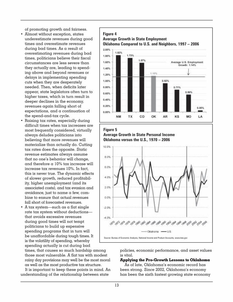
Figure 5Average Growth in State Personal IncomeOklahoma versus the U.S., 1970 – 2006

Source: Bureau of Economic Analysis, National Income and Product Accounts, www.bea.gov

13

of promoting growth and fairness.• Almost without exception, states

underestimate revenues during goodtimes and overestimate revenuesduring bad times. As a result ofoverestimating revenues during badtimes, politicians believe their fiscalcircumstances are less severe thanthey actually are, leading to spend-ing above and beyond revenues ordelays in implementing spendingcuts when they are desperatelyneeded. Then, when deficits laterappear, state legislators often turn tohigher taxes, which in turn result indeeper declines in the economy,revenues again falling short ofexpectations, and a continuation ofthe spend-and-tax cycle.

• Raising tax rates, especially duringdifficult times when tax increases aremost frequently considered, virtuallyalways deludes politicians intobelieving that more revenues willmaterialize than actually do. Cuttingtax rates does the opposite. Staticrevenue estimates always assumethat no one’s behavior will change,and therefore a 10% tax increase willincrease tax revenues 10%. In fact,this is never true. The dynamic effectsof slower growth, reduced profitabil-ity, higher unemployment (and itsassociated costs), and tax evasion andavoidance, just to name a few, com-bine to ensure that actual revenuesfall short of forecasted revenues.

• A tax system—such as a flat singlerate tax system without deductions—that avoids excessive revenuesduring good times will not temptpoliticians to build up expensivespending programs that in turn willbe unaffordable during tough times. Itis the volatility of spending, wherebyspending actually is cut during badtimes, that causes so much hardship amongthose most vulnerable. A flat tax with modestrainy day provisions may well be the most moralas well as the most productive tax structure.It is important to keep these points in mind. An

understanding of the relationship between state

policies, economic performance, and asset valuesis vital.Applying the Pro-Growth Lessons to Oklahoma

As of late, Oklahoma’s economic record hasbeen strong. Since 2002, Oklahoma’s economyhas been the sixth fastest growing state economy

Figure 4Average Growth in State EmploymentOklahoma Compared to U.S. and Neighbors, 1997 – 2006

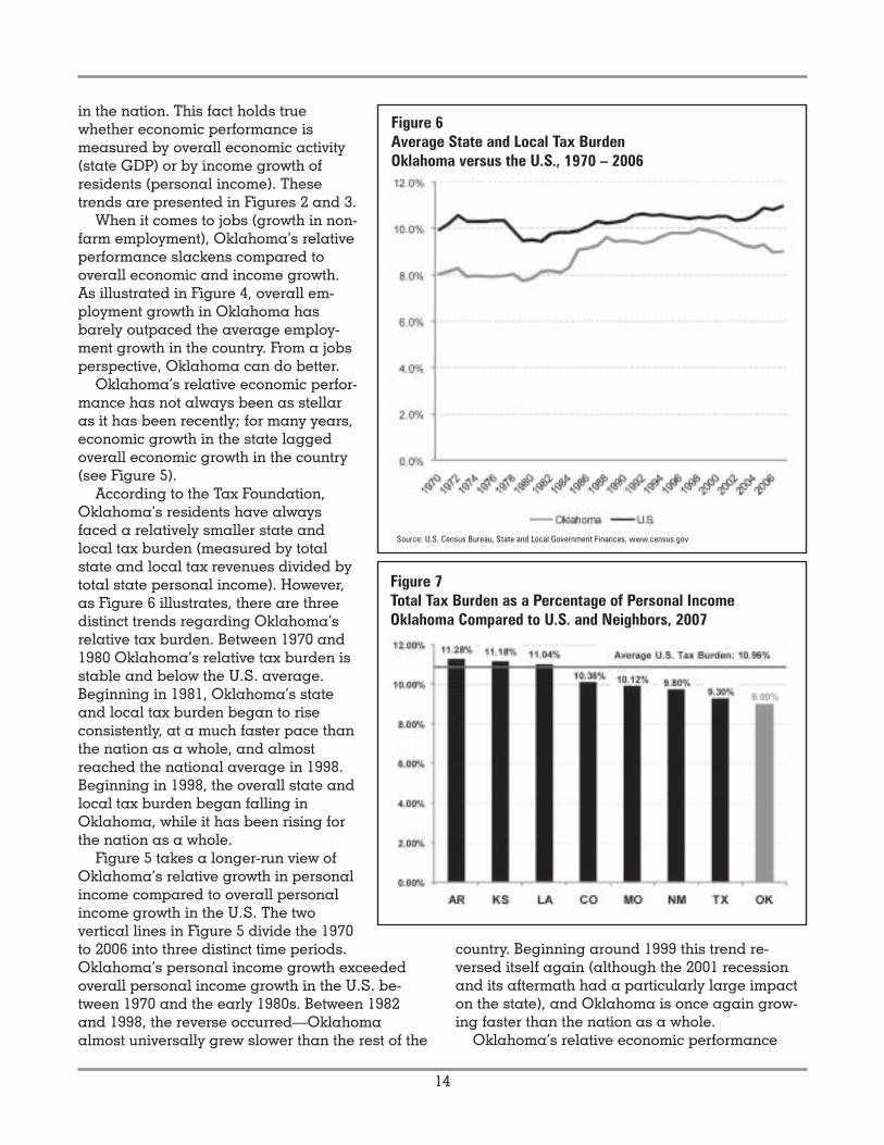
Figure 6Average State and Local Tax BurdenOklahoma versus the U.S., 1970 – 2006

Source: U.S. Census Bureau, State and Local Government Finances, www.census.gov

in the nation. This fact holds truewhether economic performance ismeasured by overall economic activity(state GDP) or by income growth ofresidents (personal income). Thesetrends are presented in Figures 2 and 3.

When it comes to jobs (growth in non-farm employment), Oklahoma’s relativeperformance slackens compared tooverall economic and income growth.As illustrated in Figure 4, overall em-ployment growth in Oklahoma hasbarely outpaced the average employ-ment growth in the country. From a jobsperspective, Oklahoma can do better.

Oklahoma’s relative economic perfor-mance has not always been as stellaras it has been recently; for many years,economic growth in the state laggedoverall economic growth in the country(see Figure 5).

According to the Tax Foundation,Oklahoma’s residents have alwaysfaced a relatively smaller state andlocal tax burden (measured by totalstate and local tax revenues divided bytotal state personal income). However,as Figure 6 illustrates, there are threedistinct trends regarding Oklahoma’srelative tax burden. Between 1970 and1980 Oklahoma’s relative tax burden isstable and below the U.S. average.Beginning in 1981, Oklahoma’s stateand local tax burden began to riseconsistently, at a much faster pace thanthe nation as a whole, and almostreached the national average in 1998.Beginning in 1998, the overall state andlocal tax burden began falling inOklahoma, while it has been rising forthe nation as a whole.

Figure 5 takes a longer-run view ofOklahoma’s relative growth in personalincome compared to overall personalincome growth in the U.S. The twovertical lines in Figure 5 divide the 1970to 2006 into three distinct time periods.Oklahoma’s personal income growth exceededoverall personal income growth in the U.S. be-tween 1970 and the early 1980s. Between 1982and 1998, the reverse occurred—Oklahomaalmost universally grew slower than the rest of the

14

country. Beginning around 1999 this trend re-versed itself again (although the 2001 recessionand its aftermath had a particularly large impacton the state), and Oklahoma is once again grow-ing faster than the nation as a whole.

Oklahoma’s relative economic performance

Figure 7Total Tax Burden as a Percentage of Personal IncomeOklahoma Compared to U.S. and Neighbors, 2007

over the past 37 years has not been random. Asthe theories described above illustrate, states thatimpose rising tax burdens experience decliningeconomic growth, and states that reduce taxburdens experience increasing economic growth.Oklahoma exemplifies this relationship since 1970.

Combining the results of Figures 5 and 6, thethree distinct periods evident in Figure 5 arealigned with the three distinct periods in Figure 6.When Oklahoma’s tax burden is rising relative tothe national average, the state’s economy isunderperforming the national average; con-versely, when Oklahoma’s tax burden is fallingrelative to the national average, the state’seconomy is outperforming the national average.Going forward, tax and spending reforms shouldbe implemented that leverage these lessons fromOklahoma’s state tax policy history.

From an overall perspective, compared to otherstates’ tax and regulatory policies, Oklahoma’stax policies are solid. However, there are areas forimprovement. Addressing these areas will helpensure the positive economic outcomes thatOklahoma has been experiencing continue, asopposed to reversing to the poorer economicperformance of the past.Oklahoma’s Tax Burden

While Oklahoma’s tax system has been improv-ing, and its tax burden as a percentage of stateincome has fallen, there are a variety of concerns.Additionally, other states in Oklahoma’s region(especially Texas) have very competitive taxsystems. In consequence, it is important to seehow Oklahoma’s tax system stacks up in its regionand nationally.

As Figure 6 illustrates, Oklahoma imposes arelatively small state and local tax burden on itscitizens. According to the Tax Foundation, totalstate and local taxes comprised 9.0% of totalpersonal income in 2007, which is the sixth smallesttax burden in the nation and substantially smallerthan all of Oklahoma’s neighbors (see Figure 7).27

Top Marginal Personal Income Tax Rate

While Oklahoma’s overall tax burden is verycompetitive, the state’s top marginal income taxrate is less so. Compared to Oklahoma’s neigh-bors, four states (Arkansas, Kansas, Missouri, andLouisiana) have higher top marginal income taxrates, but three states (New Mexico, Colorado, andTexas) have lower top marginal income tax rates(see figure 8). Oklahoma’s top marginal incometax rate is also higher than the average top

marginal income tax rate in the nation by over0.16 percentage points or $1.60 in higher taxes forevery $1,000 earned.

Top marginal income tax rates are not neces-sarily comparable. For instance, California’s toprate does not apply until an income of $1 million,while Pennsylvania imposes a flat income tax of3.07%. The median top bracket becomes effectiveonce an income of $25,000 has been reached.

Ideally, states will tax the largest possible taxbase at the lowest possible tax rate. Personalincome tax codes often fall far short of this eco-nomic ideal. Despite the fact that both mightgenerate a similar revenue stream, the tax struc-ture of a state which imposes a low flat-rate tax ona broad range of personal income providesgreater economic efficiency and growth incentives,and subsequently experiences greater economicperformance than the tax structure of a state witha narrow, highly progressive personal income tax.

Oklahoma’s top bracket becomes effective at$8,700 of income. Since that’s below the annualsalary for someone earning minimum wage, mostpeople face a flat 5.65% marginal income tax formost of their income earned.Sales Tax Rate and Burden

Due to the differences in state sales tax basesand the complexity that local sales taxes add, wecompare Oklahoma’s sales tax burden using twodifferent measures: state and local sales taxrates, and state and local sales tax revenues per$1,000 of personal income. Table 4 comparesOklahoma’s state and local sales tax rate to itsneighbors based on the lowest combined stateand local sales tax rates, as well as the highestcombined state and local sales tax rates.

15

Table 4Minimum and Maximum State and Local Sales Tax RatesOklahoma Compared to U.S. and Neighbors, 2007

Minimum State Maximum Stateand Local Sales and Local Sales

Tax Rate Tax RateArkansas 6.00% 11.50%Colorado 2.90% 9.90%Kansas 5.30% 8.30%Louisiana 4.00% 10.75%Missouri 4.28% 8.98%New Mexico 5.13% 7.88%Oklahoma 4.50% 10.50%Texas 6.25% 8.25%U.S. Average 5.00% 7.01%

When the areas with the minimumstate and local sales tax rates arecompared, Oklahoma’s minimum stateand local sales tax rate of 4.50% com-pares favorably both to the averageU.S. rate and to its neighbors—the onlyneighbors that have lower minimumstate and local sales tax rates areColorado, Louisiana, and Missouri.However, when comparing those locali-ties with the highest state and localsales tax rates, Oklahoma looks lessfavorable. Oklahoma’s localities withthe highest combined state and localsales tax rates (10.5%) are above thenational average, and only two states(Arkansas and Louisiana) have ahigher maximum combined state andlocal sales tax rate.

Total sales tax revenue per $1,000 ofpersonal income provides a measure ofthe pervasiveness of the low versus highcombined state and local sales taxrates. Figure 9 compares the sales taxburden per $1,000 of personal income inOklahoma to its neighbors, as well as theU.S. average.

Figure 9 illustrates that Oklahomaand its neighbors impose a relativelyhigh sales tax burden compared to thecountry as a whole. However, Oklahoma’soverall tax burden is well below thestates with the highest burdens—Louisiana, Arkansas, and New Mexico.Combination Tax Rate

The above review of the main statetax revenue sources—individual incometaxes and sales taxes—does not pro-vide an immediate answer with respectto which state has a more competitivetax system. In order to grasp this morefully we have constructed a “combina-tion” tax index in Tables 5 and 6. The combinationtax index shows the marginal tax bite for themajor tax systems (personal income and salestaxes) combined.28

The combination tax would be appropriate fora wage earner or someone who is receivingincome that does not pass through the Oklahoma(or other states) corporate income tax system. InOklahoma, a person earning above $8,700 a yearwould confront a 5.65% top marginal income tax

rate, and when this after-tax income is consumed,would have to confront the state and local salestaxes between 4.50% and 10.50%. According tothe Tax Foundation, the weighted average localtax rate in Oklahoma is 2.39%, for a total stateand local sales tax burden of 6.89%. The rates forOklahoma and its neighbors are summarized inTable 5.

Based on the values in Table 5, we calculatethe combination tax. The combination tax

16

Figure 8Top Marginal Personal Income Tax RateOklahoma Compared to U.S. and Neighbors, 2007

Figure 9State and Local Sales Tax Burden per $1,000 of Personal Income,Oklahoma Compared to U.S. and Neighbors, 2007

calculates the amount of money that the state andlocal income and sales taxes take for every $100of earnings in the respective states, assuming thatthe income earnings face the highest state mar-ginal income tax rate. The average state andlocal sales tax rate is adjusted because not allincome is spent on goods and services that pay astate and local sales tax, and this percentagevaries by state. Total state sales tax rates areadjusted based on each state’s sales tax base asa percentage of GDP. For instance, in Oklahoma,the 4.5% state sales tax rate raised $1.8 billion in2006.29 This implies a sales tax base of $40 billion.Total state GDP in Oklahoma was $134.7 billion in2006. Consequently, the sales tax base was 29.7%of total state GDP. The 29.7% figure is applied tothe combined state and local sales tax rate toaccount for the 70% of all income in Oklahoma

that is not part of the state sales tax base.The results of the personal combination tax are

summarized in Table 6. In Oklahoma, when aperson facing the top state marginal income taxrate earns $100, he must pay the personal incometax of 5.65%, or $5.65 in income taxes. This leavesthe person with $94.35 of income (disregardingthe effect of federal taxes). The 6.89% state andlocal sales tax (applied to 29.7% of all income)subtracts another $1.92, leaving $92.42 in after-taxincome for the individual.

Oklahoma ranks in the middle of the regiontaking 7.58% of each marginal dollar earnedthrough income and sales taxes, based on thecombination tax rate. Perhaps more troubling,Oklahoma’s combination tax is very uncompetitivecompared to Texas and Colorado. Additionally,according to the personal combination tax,Oklahoma exceeds the national average by 0.09percentage points.

Entrepreneurs, as opposed to locating inOklahoma, could settle in Texas, where thecombination marginal tax rate is significantly lessthan the tax rates they would face in Oklahoma.Or our entrepreneurs could settle in Colorado,where the combination tax rate is about 24%smaller. The comparison of Oklahoma’s combina-tion tax rates indicates that the state should lowerthese costs in order to induce more businessesand economic activity into Oklahoma.Top Marginal Corporate Income Tax Rate

As opposed to the top personal income tax rate,Oklahoma imposes a top marginal corporateincome tax rate that is below the national average.However, compared to its neighbors, Oklahoma’s

17

Table 5Combination Tax RatesOklahoma Compared to U.S. and Neighbors, 2007

Personal Weighted AverageIncome Tax State and Local

Top Rate Sales Tax Rate

Arkansas 7.00% 7.37%

Colorado 4.63% 3.83%

Kansas 6.45% 6.84%

Louisiana 6.00% 8.03%

Missouri 6.00% 7.17%

New Mexico 5.30% 5.97%

Oklahoma 5.65% 6.89%

Texas 0.00% 6.69%

U.S. 5.49% 5.94%

Table 6Combination Tax Rate Oklahoma Compared to U.S. and Neighbors, 2007

Starting Personal Income - Personal Income - PersonalPersonal Personal Personal Income Tax - CombinationIncome Income Tax Sales Tax Burden Rate

Arkansas $100.00 $93.00 $89.55 10.45%

Louisiana $100.00 $94.00 $90.65 9.35%

Kansas $100.00 $93.55 $91.25 8.75%

Missouri $100.00 $94.00 $91.81 8.19%

New Mexico $100.00 $94.70 $92.11 7.89%

Oklahoma $100.00 $94.35 $92.42 7.58%

Colorado $100.00 $95.37 $94.22 5.78%

Texas $100.00 $100.00 $98.36 1.64%

U.S. $100.00 $94.51 $92.51 7.49%

Source: ALME Calculation

top marginal corporate income tax rateis less competitive, with three neighborshaving lower top marginal income taxrates (see Figure 10).Capital Gains Taxes

Oklahoma taxes capital gains(whether they are short-term or long-term) at 5.65% (see Figure 11). Com-pared to Oklahoma’s neighbors, fourstates have higher capital gains taxes,and three states have a higher capitalgains tax on long-term capital gains.Nationally, Oklahoma’s capital gainstaxes are around 16-20 percent higherthan the average state capital gains tax.

Capital gains taxes discourageinvestment and, due to their volatility,lead to significant revenue swings forthe state. Additionally, income, sales,and severance taxes account for nearly85% of total state tax revenues. As aconsequence, the minimal amount ofrevenue that Oklahoma raises fromcapital gains taxes come at a higheconomic cost.Property Tax Burden

In 2006, Oklahoma’s property taxburden is $17.06 per $1,000 of personalincome (see Figure 12). Compared to thenation as a whole, this is the fourthsmallest property tax burden, andArkansas is the only neighbor that has asmaller property tax burden than Okla-homa. However, most of Oklahoma’sneighbors have low property tax bur-dens. The exceptions are Texas andKansas, which have higher than aver-age property tax burdens.

Oklahoma’s low property tax burdenhas played an important role in keepingOklahoma’s overall tax burden belowthe national average. As such, theproperty tax burden is a significantcompetitive advantage both nationallyand compared to the majority of its neighbors.Regulatory Burdens

Regulatory burdens can also create positive ornegative economic incentives. Burdensomeregulations that increase business costs exces-sively will tend to reduce overall economic incen-tives, while the opposite will tend to increaseoverall economic incentives. In this examination,

we focus on four regulatory-type costs that tend tohave important impacts on a state’s overalleconomic competitiveness: the state liability tortsystem, state minimum wage, worker’s compensa-tion costs, and whether the state is a “right towork” state. Overall, Oklahoma ranks belowaverage with respect to the regulatory costs thestate imposes on businesses due to the additional

18

Figure 10Top Marginal Corporate Income Tax RateOklahoma Compared to U.S. and Neighbors, 2007

Figure 11Short-term and Long-term Capital Gains Tax RatesOklahoma Compared to U.S. and Neighbors, 2007

*Texas imposes a 1.0% tax on the gross receipts on all companies (GRT). To put this rate on a comparable basis,

we scaled the Texas’ GRT up by the ratio of national income to total corporate profits, proprietor’s income and

rental income.

19

costs of its tort system and higher-than-average worker’s compensation costs.

In order to assess Oklahoma’s statetort system, ALME relied upon a tortsystem survey performed by the U.S.Chamber of Commerce. Based on thisstudy, the Laffer Associates study ranksOklahoma 38th (out of 50). This below-average rank indicates that Oklahoma’stort liability system adds greater thanaverage costs to businesses that operatein Oklahoma, compared to businessesthat operate in other states. This placesOklahoma at a distinct competitivedisadvantage when it comes to attractingbusinesses and jobs to the state.

Worker’s compensation costs imposeadditional costs on employers in Okla-homa. When employers consider hiringadditional workers, it is the total costfrom increasing employment that isrelevant, which includes all salaries,benefits, taxes, and regulatory costs.Worker’s compensation increases thecosts of employing additional workers;consequently, these regulations in-crease overall unemployment anddecrease a state’s potential economicgrowth. Oklahoma again ranks 38th (outof 50) with respect to the additionalcosts it imposes on employers due toworker’s compensation. Along with thehigher tort liability costs, the worker’scompensation costs are another barrier tobusiness and job creation in Oklahoma.

On the positive side, Oklahomamandates that businesses in the statemeet only the federal minimum wagestandard. Minimum wage laws canhave only one of two effects: either theminimum wage is below the wage thatwould be paid to any employee and isirrelevant, or the minimum wage lawraises the wage costs for employers,leading to greater unemployment. Byimposing the federal minimum wage,Oklahoma is not unnecessarily increasing em-ployer costs. In so doing, business flexibility isincreased, and overall employment in the state isenhanced.

Oklahoma is also a “right to work” state. Thislaw prohibits trade union membership from being

a prerequisite for employment, which, if allowed,would adversely affect overall employment andeconomic growth.Spending Discipline

Lastly, fiscal discipline in Oklahoma comparedto the national average has been competitive,

Figure 12Property Tax Burden per $1,000 of Personal IncomeOklahoma Compared to U.S. and Neighbors, 2007

Figure 13Growth in State Spending Per CapitaOklahoma Compared to U.S., 1978 – 2005

20

when compared over a long timeperiod. Figure 13 traces out the growthin spending per capita in Oklahomacompared to the average state spend-ing growth. As Figure 13 shows, percapita spending growth in Oklahomabetween 1978 and 2001 had beengenerally around the average stategrowth in expenditures per capita, andsometimes even below average.

However, expenditures in 2001spiked, both in absolute and relativeterms. According to the U.S. Census, thedriver of this spending spike was anincrease in public welfare expendituresthat increased from $911 million in 2000to $2.7 billion in 2001. Since the spend-ing spike in 2001, per capita spendinghas appeared to return to its typicalpattern for state and local spending;however, state spending has beengenerally above trend. Overall, state spending inOklahoma grew 8.1% between 2000 and 2005,compared to 6.3% for the average state in thenation.

Through 2005, Oklahoma’s total expendituresper capita ($4,434) were below the nationalaverage of $4,959 (see Figure 14). While such anexpenditure level is competitive on a nationalbasis, it is above average compared to several ofOklahoma’s neighbors—especially Colorado,Missouri, and Texas.

The spending discrepancy with Texas andColorado is especially disconcerting. Except forOklahoma’s lower property tax burden, Texas andColorado have lower capital gains tax rates,lower top marginal corporate income tax rates,and a lower combination tax rate (top personalmarginal income tax and sales tax). Increasingoverall tax competitiveness vis-à-vis these statesis enhanced by implementing increased spendingcontrol that brings overall spending per capita inline with Texas and Colorado—the two neighborsthat have tax systems that are more competitiveand pro-growth than Oklahoma.

Additionally, the expenditure data from the U.S.Census is only current through 2005. Since 2005,the spending record of Oklahoma has worsened,making the imperative to control spending moreurgent. Based on the 2006 Comprehensive AnnualFinancial Report, total expenditures in 2006accelerated, growing 10.1% in 2006 compared to

2005.30 Such expenditure growth worsensOklahoma’s disadvantage, compared to neigh-boring Texas and Colorado, and reduces thestate’s competitiveness vis-à-vis the remainder ofthe country. Consequently, controlling statespending is an important step for ensuring acontinuation of Oklahoma’s recent strong eco-nomic performance.

Ideas for restraining spending in Oklahomaare not wanting. For instance, the OklahomaCouncil of Public Affairs presented a detailedspending budget for FY2007 that would limitspending to a 4.2% increase (inflation plus popu-lation growth in Oklahoma).31 This proposalrepresents large potential savings that couldsignificantly help increase Oklahoma’s economiccompetitiveness.Tax Reform Suggestions

Figure 15 summarizes Oklahoma’s relativeeconomic performance and environment for 16key policy variables—which include many of thetax and regulatory policies discussed above. Asshown in Figure 15, Oklahoma’s fiscal and regula-tory policies are competitive nationally in certainareas—especially the property tax burden andrecent tax reductions. However, as discussed inmore detail above, there are areas for improve-ment. Combining the theory of pro-growth taxpolicies with our review of Oklahoma’s tax systemprovides several observations with respect to taxreform. These observations include:

Figure 14Average Expenditures per CapitaOklahoma Compared to U.S. and Neighbors, 2005

21

Figure 15. Oklahoma Fiscal and Economic Performance and Rank, 2007

22

• Oklahoma’s low overall state and local taxburden and low property tax burden are impor-tant competitive advantages for the state, whichshould be maintained.

• The state’s top marginal personal income andcorporate income tax rates are too high, espe-cially compared to neighboring Texas andColorado. Tax reforms should lower these topmarginal tax rates to bring them closer in linewith neighboring Texas and Colorado.

• The personal income tax has seven tax brack-ets, which is progressive. In general, progres-sive tax structures add significant complexity tothe tax code, while the higher top marginalincome tax rates tend to diminish pro-growthincentives throughout the economy. In Okla-homa, the top marginal personal income taxrate becomes effective at $8,700 for a singlefiler, which is less than the annual salary for afull-time minimum wage worker. The low in-come threshold for the top marginal income taxin Oklahoma creates an additional argument

for eliminating the progressive income taxstructure in Oklahoma and replacing thecomplex structure with a simpler flat tax rate.

• Oklahoma imposes a relatively high capitalgains tax rate. This rate should be reducedand, at a bare minimum, brought into line withthe capital gains taxes that are imposed inneighboring states.

• While Oklahoma’s spending record has, tradi-tionally, been competitive from a nationalperspective, overall spending has been grow-ing at a troubling pace. Furthermore, spendingper capita in the state has been above severalkey neighbors, including Texas and Colorado.In order to enhance the effectiveness of the pro-growth tax reforms suggested above, the percapita spending of state and local governmentsshould be brought in line with Texas andColorado.

—This study was conducted for OCPA by the firm

Arduin, Laffer & Moore Econometrics

(arduinlaffermoore.com).

Footnotes1George, Henry. Progress and Poverty.2 Ibid.3 Based on 2006 data across all 50 states, every 1.0 percentage

point increase in the top marginal income tax rate was associ-

ated with a reduction in total economic growth of 0.08%, on

average.4 Keynes, John Maynard (1972). The Collected Writings of John

Maynard Keynes. London: Macmillan Cambridge University

Press.5 Laffer, Arthur B. (1978). Revitalizing California’s Economy: A

Discussion of the Impact of Proposition 13. United Organization

of Taxpayers. March 22.6 ALME calculation based on data from the U.S. Census, State

and Local Government Finances, www.census.gov, and Bureau of

Economic Analysis, www.bea.gov.7 Bureau of Economic Analysis, www.bea.gov.8 Ibid.9 Bureau of Labor Statistics, www.bls.gov.10 Bureau of Labor Statistics, www.bls.gov.11 U.S. Department of Census, www.census.gov.12 U.S. Bureau of Economic Analysis; Housing prices from

California Association of Realtors, National Association of

Realtors and the Office of Federal Housing Enterprise Oversight.13 Ibid.14 U.S. Census Bureau, State and Local Government Finances,

www.census.gov.15 Ibid.16 U.S. Census Bureau, State and Local Government Finances,

www.census.gov.17 Ibid.18 Ibid.19 The White House (1963). Economic Report of the President:

Together With the Annual Report of the Council of Economic

Advisors. January.

20 Kennedy, John F. (1963). Special Message to the Congress on

Tax Reduction and Reform. January 24.21 Bureau of Economic Analysis, National Income and Product

Accounts, www.bea.gov.22 Ibid.23 Heller, Walter (1977). Testimony before the Joint Economic

Committee, U.S. Congress; quoted in Bartlett, Bruce (1978).

National Review, October 27.24 Bureau of Economic Analysis, National Income and Product

Accounts, www.bea.gov.25 Bureau of Labor Statistics, www.bls.gov.26 Bureau of Economic Analysis, National Income and Product

Accounts, www.bea.gov.27 Tax Foundation, http://www.taxfoundation.org/taxdata/.28 The combination tax rate does not account for corporate

income, dividend, and capital gains taxes. Nor does the

combination tax incorporate property taxes, which are exception-

ally low in Oklahoma. As designed, the combination tax provides

a means to compare the marginal tax rates across states for the

personal income and sales tax only.29 State Government Tax Collections Data, U.S. Census,

www.census.gov.30 Henry, Brad (2006). 2006 Comprehensive Annual Financial

Report, Fiscal Year Ended June 30, 2006. Office of State Finance.31 The Oklahoma Council of Public Affairs provides perspective

on the problems and consequences of excessive spending

growth in Oklahoma and provides a detailed budget that

allocates budget authority across departments while maintaining

the overall 4.2% expenditure cap; see Anderson, Steve, Brandon

Dutcher, and Grant Gulibon (2007). OCPA State Budget: A State

Budget That Respects Your Family Budget. Oklahoma Council of

Public Affairs.

The Oklahoma Council of Public Affairs, Inc. is anindependent, nonprofit, nonpartisan research andeducational organization devoted to improving the quality oflife for all Oklahomans by promoting sound solutions to stateand local policy questions. For more information on this

policy paper or other OCPA publications, please contact:

1401 N. Lincoln Boulevard

Oklahoma City, OK 73104

(405) 602-1667 • FAX: (405) 602-1238

www.ocpathink.org • ocpa@ocpathink.org

OCPA Trustees

Blake ArnoldOklahoma City

Mary Lou AveryOklahoma City

Lee J. BaxterLawton

Steve W. BeebeDuncan

G.T. BlankenshipOklahoma City

John A. BrockTulsa

David R. Brown, M.D.Oklahoma City

Aaron BurlesonAltus

Paul A. CoxOklahoma City

William FlanaganClaremore

Josephine FreedeOklahoma City

Kent FrizzellClaremore

John T. HanesOklahoma City

Ralph HarveyOklahoma City

John A. Henry IIIOklahoma City

Paul H. HitchGuymon

Henry F. KaneBartlesville

Robert KaneTulsa

Tom H. McCasland IIIDuncan

David McLaughlinEnid

Lew MeibergenEnid

Ronald L. MercerBethany

Lloyd Noble IITulsa

Robert E. PattersonTulsa

Russell M. PerryEdmond

Bill PriceOklahoma City

Patrick RooneyOklahoma City

Melissa SandeferNorman

Richard SiasOklahoma City

Charles SublettTulsa

Robert SullivanTulsa

Lew WardEnid

William E. Warnock, Jr.Tulsa

Gary W. Wilson, M.D.Edmond

Daryl WoodardTulsa

Daniel J. ZaloudekTulsa

OCPA Adjunct Scholars

Will Clark, Ph.D.University of Oklahoma

David Deming, Ph.D.University of Oklahoma

Bobbie L. Foote, Ph.D.University of Oklahoma (Ret.)

Kyle Harper, Ph.D.University of Oklahoma

E. Scott Henley, Ph.D., J.D., D.Ph.Oklahoma City University (Ret.)

James E. Hibdon, Ph.D.University of Oklahoma (Ret.)

Russell W. Jones, Ph.D.University of Central Oklahoma

Andrew W. Lester, J.D.Oklahoma City University (Adjunct)

David L. May, Ph.D.Oklahoma City University

Ronald L. Moomaw, Ph.D.Oklahoma State University

Ann Nalley, Ph.D.Cameron University

Bruce Newman, Ph.D.Western Oklahoma State College

Stafford North, Ph.D.Oklahoma Christian University

Michael Scaperlanda, J.D.University of Oklahoma

Andrew C. Spiropoulos, J.D.Oklahoma City University

OCPA FellowsSteven J. Anderson, MBA, CPA

Research Fellow

J. Rufus Fears, Ph.D.Dr. David and Ann Brown Distinguished Fellow

for Freedom Enhancement

Patrick B. McGuigan, M.A.Research Fellow

J. Scott Moody, M.A.Research Fellow

Wendy P. Warcholik, Ph.D.Research Fellow

OCPA Legal CounselDeBee Gilchrist � Oklahoma City

OCPA StaffHopper T. Smith / President

Brett A. Magbee / VP for OperationsBrandon Dutcher / VP for Policy

Margaret Ann Hoenig / Director of DevelopmentBrian Hobbs / Director of Marketing and Public Affairs

Sandra Leaver / Operations Assistant