Embed Size (px)
Citation preview

A testing technique for concrete under confinement at
high rates of strain
Pascal Forquin, Gerard Gary, Fabrice Gatuingt
To cite this version:
Pascal Forquin, Gerard Gary, Fabrice Gatuingt. A testing technique for concrete under con-finement at high rates of strain. International Journal of Impact Engineering, Elsevier, 2008,35 (6), pp.425-446. <10.1016/j.ijimpeng.2007.04.007>. <hal-00994320>
HAL Id: hal-00994320
https://hal.archives-ouvertes.fr/hal-00994320
Submitted on 21 May 2014
HAL is a multi-disciplinary open accessarchive for the deposit and dissemination of sci-entific research documents, whether they are pub-lished or not. The documents may come fromteaching and research institutions in France orabroad, or from public or private research centers.
L’archive ouverte pluridisciplinaire HAL, estdestinee au depot et a la diffusion de documentsscientifiques de niveau recherche, publies ou non,emanant des etablissements d’enseignement et derecherche francais ou etrangers, des laboratoirespublics ou prives.

www.elsevier.com/locate/ijimpeng
Author’s Accepted Manuscript
A testing technique for concrete under confinementat high rates of strain
P. Forquin, G. Gary, F. Gatuingt
PII: S0734-743X(07)00067-XDOI: doi:10.1016/j.ijimpeng.2007.04.007Reference: IE 1483
To appear in: International Journal of Impact
Accepted date: 25 April 2007
Cite this article as: P. Forquin, G. Gary and F. Gatuingt, A testing technique for con-crete under confinement at high rates of strain, International Journal of Impact (2007),doi:10.1016/j.ijimpeng.2007.04.007
This is a PDF file of an unedited manuscript that has been accepted for publication. Asa service to our customers we are providing this early version of the manuscript. Themanuscript will undergo copyediting, typesetting, and review of the resulting galley proofbefore it is published in its final citable form. Please note that during the production processerrors may be discovered which could affect the content, and all legal disclaimers that applyto the journal pertain.pe
er-0
0499
102,
ver
sion
1 -
9 Ju
l 201
0Author manuscript, published in "International Journal of Impact Engineering 35, 6 (2008) 425"
DOI : 10.1016/j.ijimpeng.2007.04.007

Accep
ted m
anusc
ript
1
A testing technique for concrete under confinement at high rates of strain
P. Forquin1, , G. Gary2 & F. Gatuingt3
1 Laboratoire de Physique et de Mécanique des matériaux, Université de Metz, 57045 Metz, France
2 Laboratoire de Mécanique des Solides, Ecole Polytechnique, 91128 Palaiseau, France
[email protected] - http://lmsX.polytechnique.fr/LMSX/
3 Laboratoire de Mécanique et Technologie, E.N.S. de Cachan, 94235 Cachan, France
Abstract: A testing device is presented for the experimental study of dynamic compaction
of concrete under high strain-rates. The specimen is confined in a metallic ring and loaded
by means of a hard steel Hopkinson pressure bar (80 mm diameter, 6 m long) allowing for
the testing of specimens large enough regarding the aggregates size. The constitutive law
for the metal of the ring being known, transverse gauges glued on its lateral surface allow
for the measurement of the confining pressure. The hydrostatic and the deviatoric response
of the specimen can then be computed. The proposed method is validated by several
numerical simulations of tests involving a set of 4 different concrete-like behaviours and
different friction coefficients between the cell and the specimen. Finally, 3 tests performed
with the MB50 concrete at 3 different strain rates are processed with the method and are
compared with literature results for the same material under quasi-static loadings.
peer
-004
9910
2, v
ersi
on 1
- 9
Jul 2
010

Accep
ted m
anusc
ript
2
Keywords: 1D-strain compression test, Hopkinson pressure bar, Deviatoric strength and
compaction law, High-performance concrete.
1. Introduction
Compaction of concrete with a volume decrease of 10% or more occurs under high pressures.
Such situations are found in military applications or in studies connected with the safety of
buildings (power plants) regarding an accidental internal loading or external loading (plane
crash).
On the one hand, the stress needed for compaction is high (around 1000 MPa) with a large
pressure component. On the other hand, the specimens must be large enough to be representative
with respect to the size of aggregates. Consequently, the forces required are so large that only a
few testing procedures are available in this field. In the quasi-static load regime multiaxial tests
use compression cells that are able to support very high pressures [1, 2]. Dynamic plate impact
tests are also used [3], for which the strain-rates obtainable are in the range of 105 s-1 or greater.
The testing device presented in this paper is a method of obtaining results between quasi-static
and high speed loading rates (from 200 to 2000 s-1) where only a few results involving
compaction are found.
In this range of loading pressures, the behaviour of concrete is generally described by means
of plasticity theories where the hydrostatic and the deviatoric responses are considered separately.
The major differences between different models are found in the way both responses are coupled.
Corresponding author. Tel.: +33-3-87-54-72-49; fax: +33-3-87-31-53-66; email address: [email protected]
peer
-004
9910
2, v
ersi
on 1
- 9
Jul 2
010

Accep
ted m
anusc
ript
3
A clear understanding has then to be based on well-defined loading paths. As real loading
situations leading to compaction are generally dynamic ones, the study of strain rate effects is
important.
A significant literature exists on rate the sensitivity of rock tested at medium strain rates, for
example in ancient papers [4, 5], and a more recent one [6]. The early tests on concrete under
dynamic loading were performed with pendulum and drop weight tests. An arrangement using
impulse loading of a cylindrical specimen made of concrete was used by Goldsmith and co-
workers [7] to study the tensile fracture feature of concrete. The use of the compressive Split
Hopkinson Pressure Bar (SHPB) to determine the rate sensitivity of concrete can be found in
recent works [8-12]. However, the test analysis must consider both material and geometric
aspects. For example, the increase of the stress with the strain rate can be due to the radial
confinement induced by inertia and/or by the intrinsic rate sensitivity of the material. Indeed, for
a material with a non-zero Poisson’s ratio, the lateral expansion associated with the compression
is restrained by inertia effects [13, 14, 15, 16]. As rock-like materials are very sensitive to the
lateral pressure when they are axially loaded, they can show geometry dependent strain-rate
sensitivity. In the present case, the confinement cell considerably reduces the radial displacement
so the radial pressure induced by inertia does not act.
Dynamic axial compression testing with lateral pressure is not very common. For lower lateral
pressures, experimental data have been obtained using a SHPB axial loading system combined
with a pressure cell [5, 12, 17, 18]. This technique does not produce the high pressures required
for compaction.
A new testing device has been designed and studied by Burlion et al. [2] for the case of quasi-
static loading, involving axial and lateral stresses in the range of expected dynamic values. In the
peer
-004
9910
2, v
ersi
on 1
- 9
Jul 2
010

Accep
ted m
anusc
ript
4
present work, an attempt was made to extend this technique to the dynamic range using a SHPB
to produce axial loading and to measure axial forces and displacements. Following a few authors
[12, 17, 19], we then propose a test where the specimen is confined in an instrumented metallic
ring and loaded by means of a Hopkinson pressure bar (SHPB) especially designed for this
purpose.
2. General description of the confining compression test
Specimen and Cell geometry
The general idea of the test is described in figure 1. A cylindrical specimen embedded in a
steel confinement ring is compressed using 2 cylindrical plugs (Fig. 1a). The concrete specimen
has a diameter of 30 mm and is 40 mm long. The steel plugs have the same diameter and a
thickness of 10 mm. The steel ring has an outer diameter of 65 mm and is 45 mm long.
The “MB50” concrete
The selected high strength concrete “MB50” has already been extensively studied [20, 21, 22,
23]. The specimens to be tested were machined in a concrete block after being dried (40 days) to
prevent the effects of drying shrinkage of the concrete. The composition and the mean
mechanical properties of MB50 are detailed in table 1.
peer
-004
9910
2, v
ersi
on 1
- 9
Jul 2
010

Accep
ted m
anusc
ript
5
Interface product between the specimen and the cell
A gap, about 0.2 mm thick, is left between the concrete specimen and the ring. It is filled with
an epoxy resin, coated with Teflon. This material is highly incompressible and hence does not
reduce the confinement pressure. It also has a weak shear strength allowing for easier relative
displacements between the ring and the specimen.
Direct strain measurements on the cell
Three hoop strain gauges were glued onto the external surface of the metallic ring. Their
outputs allow the deduction of the radial stress and strain within the specimen. One gauge is
located in the middle of the ring (n°2), as shown in figure 1b and the two others (n°1 and 3) are
located at a distance from the middle equal to ¾ of the half-length of the ring. Three axial gauges
(n°4, 5, 6) are located on the same axial planes (Fig. 1b). From their outputs, it is expected to
deduce the friction force between the specimen and the ring and to quantify the barrelling of the
ring.
Brief description of the test
The cell and its plugs are inserted between the two Hopkinson bars. The loading produces
compression of the concrete and a subsequent increase of the internal pressure supported by the
cylindrical cell. The signals recorded on the two Hopkinson bar gauges allow for the computation
of the axial forces and of the corresponding displacements. The signals recorded with the gauges
glued on the cell give information on its response under pressure from the concrete specimen.
peer
-004
9910
2, v
ersi
on 1
- 9
Jul 2
010

Accep
ted m
anusc
ript
6
3. The SHPB loading device
Basic description of the SHPB system
The SHPB (Split Hopkinson Pressure Bar) system, also called Kolsky's apparatus is a
commonly used experimental technique in the study of the constitutive laws of materials at high
strain rates. The first use of a long thin bar to measure stresses under impact conditions has been
reported in [24]. The experimental set-up with two long bars, widely used today, was pioneered
by Kolsky [25].
A typical SHPB testing device is composed of long input (or incident) and output (or
transmitter) bars with a short specimen placed between them. With the impact of a projectile (or
striker) at the free end of the input bar, a compressive longitudinal "incident" wave ( )tIε is
created in the input bar. Once the incident wave reaches the interface between the specimen and
the bar, a reflected pulse ( )tRε in the input bar and a transmitted pulse ( )tTε in the output bar are
developed. With the gauges that are glued on the input and output bars (named A and B,
respectively), these three basic waves are recorded. Their processing allows for the knowledge of
forces and particle velocities at both faces of the specimen [25].
Recall of the processing technique
As both the incident and the reflected waves have to be known, the optimal position of a single
peer
-004
9910
2, v
ersi
on 1
- 9
Jul 2
010
Accep
ted m
anusc
ript
7
gauge station “A” that allows for the longest loading time is the middle of the input bar. The
maximum theoretical length of the striker is then half the length of the input bar. In fact, because
of the non-zero rising time of the incident wave, the length of the striker has more often to be
around 80% of the theoretical one.
The forces and the particle velocities at the specimen faces are calculated with waves shifted
to the same points. For slender elastic bars, it is assumed that the elastic waves propagate without
dispersion so that they are simply time shifted to the bar ends.
Let us call )(tiε , )(trε and )(ttε the corresponding (shifted) waves. For the sake of simplicity,
a one-dimensional analysis gives the usual relations between jumps of stress (∆σ), particle
velocity (∆v) and strain (∆ε) [26], when a single direction of propagation is considered.
∆σ = ±ρc∆v , (1a)
and, in the 1-D purely elastic case
/v cε∆ = ±∆ (1b)
where c is the bar wave speed (c = (E/ρ)1/2) of a 1-D wave propagating in the bars. Using these
equations together with the superposition principle, the velocities and the forces at both specimen
faces are given by the following formulas (2a and 2b).
Vin (t) = −c(εi(t) −εr(t))
Vout (t) = −c(εt (t)), (2a)
Fin (t) = Sb E(εi(t) + εr (t))
Fout (t) = Sb Eεt (t), (2b)
peer
-004
9910
2, v
ersi
on 1
- 9
Jul 2
010

Accep
ted m
anusc
ript
8
where V is the velocity, F the force, bS the area of the bars, E the Young's modulus of the bars.
Subscripts in and out indicate the input and output sides, respectively.
Present SHPB device and processing technique
The SHPB set-up (striker, input bar and transmitter bar) used here is made of steel bars (elastic
limit 1200 MPa) with a diameter of 80 mm. The striker, the input bar and the output bar are 2.2m,
6m and 4 m long, respectively. The strains at points A (middle of input bar) and B (1 m away
from the specimen) are measured with strain gauges. Considering the elastic response of the bar
and assuming a uniaxial state of stress at the gauges stations, an improved measurement of the
strain is made by using a complete gauge bridge. At the given position of the gauge station, each
couple of transverse and longitudinal gauges are diametrically opposed on the surface of the bar
to eliminate a possible bending component of the strain. The transverse strain is equal to the
longitudinal strain multiplied by the Poisson's ratio. The gauges that are used are “2mm, Kyowa -
KSN-2-120-F3-11” type. The bridge is supplied by a monitored 8 Volts supply and the signals are
amplified (amplifier gain 100-200-500-1000, six channels, bandwidth 200 kHz). They are then
recorded with a data acquisition card (12 bits) with the time base set to the value of 1 µs.
Knowing that the wave speed is equal to 5120 m/s, it can be simply deduced from the dimensions
of the set up that the loading pulse duration is equal to 860 µs. The beginning of the reflected
wave arises 300 µs later than the end of the incident pulse. Both waves are thus easily separated
(Fig. 2).
The shifting of the waves to the specimen ends takes account of dispersion. We use a
dispersion relation that is the first mode solution of the Pochhammer [27] and Chree [28]
peer
-004
9910
2, v
ersi
on 1
- 9
Jul 2
010

Accep
ted m
anusc
ript
9
equation, computed for the material constants of our bars. Since the bars have an unusually large
diameter, it is worth checking that only the first mode is involved. A spectral analysis of the
gauge signals recorded shows a negligible amplitude for frequencies greater than 20 kHz. The
cut-off frequency of the second mode is, in the case of our bars, close to the same value (from
Davies [29] it is known that the minimum phase velocity for the second mode corresponds to
25.0=Λa and the minimum group velocity corresponds to 3.0=Λ
a where a is the radius of
the bar and Λ the wavelength. Here, a and c (equation 1) are equal to 0.04 m and 5120 m/s
respectively. The corresponding cut-off frequencies are equal to 32 kHz and 38.4 kHz
respectively). An easy check of the quality of the dispersion correction can be performed by the
long distance travel of a wave using the input bar with both free ends after the loading (as shown
in [30, 31]).
It was also checked that below 20 kHz, the proportionality of lateral and longitudinal strain is
true to better than 99% (from Tyas and Watson [32]) taking account of the energy spectrum of
our waves. A complete bridge involving lateral and axial strains can then be safely used for this
measurement.
For precise time shifting, an assisted delay setting method was used. This is based on the
existence of an initial elastic response of the specimen. During the corresponding time, real
reflected and transmitted waves are compared with theoretical ones computed from the
knowledge of the incident wave and an assumed elastic behaviour of the specimen [33, 30]. This
data processing method ensures precise measurements at low strains (in the range of strains lower
than 1%) [11].
Using equations (2), the forces and the velocities (and the displacements, by integration) at
both sides of the complete specimen (including the plugs) are calculated. These data are the
peer
-004
9910
2, v
ersi
on 1
- 9
Jul 2
010

Accep
ted m
anusc
ript
10
results of a one-dimensional analysis. The force is the integral of the axial stress over the
specimen area while the velocity is the mean velocity of the bar end.
The compression device used for dynamic testing
The device used for dynamic testing was briefly described in figure 1. The complete cell
composed of the specimen, the steel ring and the plugs is inserted between two Hopkinson bars.
It would have been easier to use a cell with the same inner diameter as bars and avoid the use of
plugs. However, to produce the expected axial stress level (evaluated from quasi-static test
results) of -1000 MPa, the value of the striker speed of a steel SHPB needed in this case should
have been 50 m/s. We have experienced that such a striker speed induces the unsticking of the
strain gauges and for this reason it is necessary to keep the striker speed under 20 m/s. A
reduction of area between the specimen and the bar is therefore necessary. This explains the
design dimensions of the bars and of the specimen and the use of steel plugs.
The elastic limit of the plugs is higher than the maximum stress obtained in our tests and the
elastic shortening of the plugs can easily be subtracted from the total shortening measured.
For a more precise correction, a test with the two plugs alone was performed within the range
of the maximum force observed in tests with the complete device. From the corresponding
relation between the force and the displacement, a lower Young’s modulus than that for steel was
found. The reason is that the total average displacement (regarding the section of the bar) is the
sum of the elastic compression of the plugs and the local elastic punching of bar ends. This needs
to be subtracted from the displacement measured in the tests with the complete device.
peer
-004
9910
2, v
ersi
on 1
- 9
Jul 2
010
Accep
ted m
anusc
ript
11
4. A method to measure states of stress and strain during
confined 1D-strain compression tests
At high stress levels, a high axial strain and rather small (but not negligible) radial strain of the
specimen are observed. In order to evaluate the compaction law of the concrete, an accurate
measurement of the state of stress and strain within the specimen is needed. For this, one first
needs to know the elastic (and possibly elastoplastic) behaviour of the material of the ring. The
identification of the mechanical behaviour of this material is presented in subsection 4.2.
The complete method used to compute the mechanical behaviour of the sample is explained in
subsection 4.3. With this method, the state of strain and stress is measured knowing, on the one
hand, the axial forces and displacements at the specimen end surfaces and, on the other hand, the
outer strain of the ring. The lateral pressure between the ring and the specimen is deduced from
the strains measured on the ring and is corrected for the real length of the specimen. The axial
stress is computed from the axial forces taking into account the (small) lateral expansion - the
radial strain - of the specimen.
Several numerical simulations were performed and are presented in subsection 4.4 with
different sets of parameters for the Krieg, Swenson and Taylor model with 2 friction coefficients
to validate the method and its robustness. In the section 5, this method is applied to three 1-D-
strain compression tests.
peer
-004
9910
2, v
ersi
on 1
- 9
Jul 2
010

Accep
ted m
anusc
ript
12
4.1. BASIC ANALYSIS
Considering that the cell is elastic and that its cylindrical shape is undeformed (that means that a
possible barrelling effect is neglected), a basic analysis of the test can be done. The hoop external
strain ( extθθε ) and the internal pressure (Pint) are related in the following way (formula valid for an
infinite cylinder):
)(
222
2int
ie
i
c
ext
RRR
EP
−=θθε , (3)
where Ec, Ri, Re are the Young’s modulus of the cell and the inside and outside radius of the cell,
respectively.
The length of the specimen will vary during the test, so that friction forces will appear
between the specimen and the cell. These forces will contribute to the overall compression force
measured by the SHPB. They also should induce an axial strain in the cell. Assuming a state of
equilibrium of the cell and a constant friction force, the loading can be described with two
opposite and symmetric homogeneous axial forces acting along the internal diameter of the cell.
The subsequent axial strain within the steel ring will decrease (in absolute value) from the
middle, where its value is equal to fraxial
maxε , to zero at the specimen ends. In that case, one has:
max 2 2int
1 /( )axial i e ifrc
f P R H R RE
ε = − , (4)
where H is the height of the cell and f the friction coefficient.
Following this elementary analysis, the internal pressure and the friction forces could then be
peer
-004
9910
2, v
ersi
on 1
- 9
Jul 2
010

Accep
ted m
anusc
ript
13
measured and the axial stress could be calculated from the global force and from the friction
forces. The main difficulty with this analysis is that it needs a cell thin enough to provide
measurable strains (due to friction) but also a cell thick enough to prevent barrelling. It is shown
in the following that both requirements cannot be met and that the processing of the strain data
measured on the cell must be more sophisticated.
4.2. IDENTIFICATION OF THE BEHAVIOR OF THE STEEL OF THE
CELL
The behaviour of the steel used for the ring component was identified by means of two dynamic
compression tests performed at strain rates of approximately 200 s-1 and 300 s-1. The strong strain
hardening and the high failure strain observed (Fig. 3) allow avoiding any strain localisation
within the steel ring. The plastic behaviour of the steel is described by a piece-wise linear law
(Fig. 3). It is assumed to be the same for any part of the cell. The Young’s modulus is taken equal
to 2x10⁵ MPa.
4.3. NUMERICAL ANALYSIS OF THE RESPONSE OF THE CELL FOR
THE TEST ANALYSIS
In order to analyse the response of the cell submitted to internal pressure and friction forces
numerical simulations were undertaken. They take account of the variable axial length where the
pressure is applied (simulating the change of the specimen length during the loading) and of the
elastoplastic behaviour of the cell.
peer
-004
9910
2, v
ersi
on 1
- 9
Jul 2
010

Accep
ted m
anusc
ript
14
4.3.1 Strains induced by a uniform pressure applied to the inner surface of the cell
First, it was determined how the pressure applied by the concrete to the inner surface of the cell is
related to the hoop strain measured at its outer surface. To do so, numerical simulations of the
cell loaded by an internal pressure were carried out using the finite element computer code
Abaqus Implicit [34]. A similar approach had previously been successfully applied to a smaller
steel ring whose elastic limit was lower [35]. The computations showed a noticeable barrelling of
the cell. In the present case, the geometry of the cell was as described before (outer diameter 65
mm, inner diameter 30 mm and height 45 mm). Two numerical simulations were carried out to
take account of the change in length of the specimen during the test. In both cases, a radial
compressive stress was applied to the inner surface (cylindrical). In the first case, this pressure
was applied to a central part of the cell 40 mm long (smaller than the cell length), equal to the
initial length of the sample. In the second numerical simulation, the pressure was applied to a
shorter central part 34 mm long (equal to the specimen length at the end of the test in the case of
a nominal axial strain equal to -15%). This value is close to the ultimate level of strain that is
reached during the tests. The two curves (internal-radial-stress versus external-hoop-strain) are
plotted in figure 4. A linear interpolation between these 2 results is used to take account of the
real length of the sample during the test. The length of the specimen is directly deduced from
SHPB data.
From both simulations, it was shown that the cell remains in the elastic range when the
internal pressure is lower than approximately 300 MPa, and the external hoop strain is
approximately lower than 0.1%. Anyway, the post-processing of the data proposed below, based
on the interpolation between the above loadings, is still possible when the cell is plastically
peer
-004
9910
2, v
ersi
on 1
- 9
Jul 2
010
Accep
ted m
anusc
ript
15
loaded. In such a case, the same cell could not be used more than once.
The radial inner stress (int)radialσ is related to the measured outer hoop strain εθθ
(z=0, ext) in the
following way:
(int) ( 0, ) ( 0, ) ( 0, )( , ) 1 ( ) ( )z ext z ext z extaxial axialradial axial A B
B Bθθ θθ θθ
ε εσ ε ε σ ε σ εε ε
= = = − = − +
, (5)
where Aσ and Bσ are the functions identified from figure 4, associated with a null strain
(specimen length 40 mm) and a strain Bε equal to 0.15 (specimen length 34 mm), respectively. It
will be assumed in the following that the radial stress is homogeneous in the sample and
consequently is equal to the radial stress applied by the sample to the cell ( (int) Sradial rrσ σ= ).
Moreover, in the above simulations, the strains (and stresses) can be calculated at any
point in the cell. Fig. 5 shows the evolution of the inner hoop strain at points (z = 0, the axial
symmetry plane and z = h0/2, the initial specimen ends) for both simulated loading cases (A and
B) as a function of the external hoop strain (εθθ(z=0, ext)). It appears (as expected) that the barrelling
effect is stronger in case B (hpress = 34 mm) than in case A (hpress = 40 mm).
It is then possible to compute the average inner hoop strain along the specimen height
(between z = 0 to z = hspecimen/2) knowing the outer hoop strains measured on the cell and the
axial strain of the specimen. The average radial strain of the specimen being known, the average
specimen area may be also computed as a function of the outer hoop strain (εθθ(z=0, ext)):
( 0, )0 (1 ( ))z ext
sA A f θθε == +
The average axial stress is then:
peer
-004
9910
2, v
ersi
on 1
- 9
Jul 2
010

Accep
ted m
anusc
ript
16
s
axialSZZ A
F=σ , (6)
This value axialF is not directly computable by the SHPB analysis as the force deduced
from SHPB measurements also includes the force induced by friction mechanisms. In order to
evaluate the importance of the corresponding friction force, new simulations were made: the cell
is loaded with a uniform shear stress combined with the uniform pressure previously applied to
the inner surface.
4.3.2 Effect of a uniform shear stress applied to the inner surface of the cell in addition to the
internal pressure
The above simulations confirm that the internal pressure induces a barrelling of the ring.
Friction between the specimen and the ring would also induce barrelling. It is thus important to
check how such friction could modify the value of the external hoop strain from which the
internal pressure is calculated. Furthermore, as explained in subsection 4.1, the friction forces
would induce an overestimation of the axial stress in the specimen if the stress level was directly
deduced from the axial force given by standard SHPB analysis.
So, in the simulation, shear stresses were applied, in addition to the internal pressure. These
shear stresses were set to be equal to 10% of the normal stress (corresponding to a friction
coefficient equal to 0.1). They are imposed via nodal forces (for reasons of convenience) in the
direction –z (for z > 0), so the direction of these nodal forces does not change with the cell
deformation. The result of one simulation (with shear) is illustrated in figure 6 showing the
evolution of the internal pressure according to the outer hoop strain (a slope of pressure from 0 to
peer
-004
9910
2, v
ersi
on 1
- 9
Jul 2
010

Accep
ted m
anusc
ript
17
800 MPa and shear stress from 0 to -80 MPa were applied over a height hpress of 40 mm). This
curve is compared with the first simulation without friction previously presented in figure 4.
It is observed that, for the same outer hoop strain, the radial stress is decreased by 3 to 5%
when friction is added to the internal pressure. Neglecting the friction would then lead to a
slightly overestimated internal pressure deduced from the external hoop strain. It is explained, in
other words, by the fact that the barrelling of the cell, and consequently the external hoop strain,
is increased by the shear at a given pressure.
As it is planned to measure the friction from the axial strain at the outer surface, figure 7 shows a
comparison of the ratio between the external axial strain and the hoop strain at the measuring
middle point (z = 0) with and without friction, for a height of the loaded area equal to 34 and 40
mm. The results are plotted as a function of the internal pressure increasing from 0 to 600 MPa
(the pressure range observed during the tests will be given latter). The axial strain at measuring
points n°4 or n°6 (z = 3H/8) appears very small. Consequently, it was not used in the data
processing.
The external axial strain appears to be much more influenced by the height of the loaded area
than by the amplitude of the friction, so that it seems difficult to evaluate friction from the outer
axial strain of the cell. However, figure 7 shows some indications about how the friction might be
evaluated from the axial strain. For example, if the internal pressure was lower than 300 MPa
(elastic deformation of the cell) and if a small axial strain of the specimen was considered (hpress
= 40 mm), the outer axial strain would appear negative without friction or positive if friction
forces were acting. In fact, a negative axial strain is the consequence of the uniaxial stress state
that exists close to the outer surface of the specimen (because σθθ > 0, σzz ≈ σrr ≈ 0) whereas a
positive axial strain is the result of the barrelling deformation due to friction. In contrast to the
peer
-004
9910
2, v
ersi
on 1
- 9
Jul 2
010

Accep
ted m
anusc
ript
18
simple analytical solution (equation 4), friction is seen to induce a positive increment of axial
strain.
The same figure shows that, if an internal pressure higher than 300 MPa is considered, the axial
strain level is strongly influenced by the height of the loaded area and weakly by the magnitude
of the friction. In this case, the ratio between the measured hoop strains at points 1 and 2 appears
more reliable (figure 8).
The ratio between the hoop strains measured ( ( 3 /8, ) ( 0, )/z H ext z extθθ θθε ε= = ) is as much influenced
by the friction as by the internal height of the loaded area (figure 8). Nevertheless, the level of the
remote hoop strain is much higher than that of the axial strain and the sensitiveness of the
measure is increased. If the internal pressure is less than 300 MPa (elastic deformation of the cell)
and if the axial strain of the specimen is lower than a few percents (hpress = 40 mm), the ratio of
hoop strains will be equal to 0.84 without friction and to 0.76 with friction. It corresponds to a
decrease of 9% due to friction. If the internal pressure is equal to 600 MPa, the ratio of hoop
strains decreases to 0.70 (hpress = 40 mm) or 0.57 (hpress = 34 mm). So, knowing the internal
pressure applied and the axial strain of the specimen, the ratio of hoop strains could be used to
evaluate the magnitude of the friction.
These observations show that an extra "barrelling" deformation is generated by a shear
stress applied along the inner surface. This deformation leads to an increase of the difference
between the outer hoop strains measured (εθθ(z=3H/8, ext), εθθ
(z=0, ext)) and an increase of outer axial
strain (εzz(z=0, ext)). Moreover, a friction coefficient of 0.1 between the cell and the sample can
induce a slight over-estimation of the inner radial stress (of approximately 4%) and of the inner
hoop strain (of approximately 6%) not detailed above.
peer
-004
9910
2, v
ersi
on 1
- 9
Jul 2
010

Accep
ted m
anusc
ript
19
4.3.3 Evaluation of the possible influence of friction forces (added to the force resulting from
pure axial stresses) on the computed specimen behaviour
As explained before, the friction leads to an over-estimation of the axial stress. The
corresponding maximum relative error can be related to the contact forces:
222( )
4
fr rrax rr
zzax zz
zz
hD fF hErr fDF D
π σ σσσπ σ
= = = , with
P
Pdev
dev
zz
rr
σ
σ
σσ
321
311
+
−= (7, 8)
where f is the friction coefficient, h and D the height and the diameter of the sample respectively.
σrr and σzz, are the average radial stress and the axial stress in the sample, respectively. So, the
corresponding error can be evaluated knowing the geometry of the specimen, the friction
coefficient and the ratio between the deviatoric strength and pressure. The smaller this ratio, the
higher is the error (equations 7 and 8). The tests that are presented later in the paper show that the
ratio (σdev/P) always remained above 0.9. Therefore, the maximum ratio between the radial stress
level and the axial stress level is approximately 0.44 (equation 8). If the initial dimensions of the
specimen are considered (h = 40 mm, D = 30 mm) it appears that the relative error in the axial
stress induced by a friction coefficient f is always under 1.2f (i.e. 12% if f = 0.1, equation 7). The
numerical simulations done with and without friction will give a more precise evaluation of the
error that could arise from neglecting the friction.
4.3.4 Computation of the mechanical fields involved in the material behaviour
The radial stress being known, the average deviatoric stress is:
peer
-004
9910
2, v
ersi
on 1
- 9
Jul 2
010

Accep
ted m
anusc
ript
20
S S Sdeviatoric zz rrσ σ σ= − , (9)
the average hydrostatic pressure and the volumetric strain are given by the formulas:
( )1 23
S S Shydrostatic zz rrP σ σ= − + , (10)
2(1 )(1 ) 1S Svolumic axial rrε ε ε= + + − . (11)
Knowing the axial stress and the internal pressure, the deviatoric behaviour (i.e. the supposed
evolution of the deviatoric stress versus the hydrostatic pressure) and hydrostatic behaviour
(variation of the volumetric strain versus the hydrostatic pressure) can be calculated.
4.4. A NUMERICAL VALIDATION OF THE METHOD
In order to check the validity of the proposed method used to process the experimental data,
artificial experimental tests were performed using numerical simulations. These simulations use
the concrete plasticity model (the KST model, see underneath) with 4 different sets of parameters
in order to evaluate a large enough range of possible behaviours. Meanwhile, the main hypothesis
introduced in subsection 4.3 will be justified (influence of the specimen shortening, of the cell
expansion, and of the friction coefficient).
This material model is not rate-sensitive. In the dynamic range, very small rate sensitivity for the
tested concrete will be demonstrated (chapter 5) that validates the present assumption.
4.4.1 The Krieg, Swenson and Taylor (KST) model
peer
-004
9910
2, v
ersi
on 1
- 9
Jul 2
010

Accep
ted m
anusc
ript
21
The model of Krieg, Swenson and Taylor [36, 37] is relatively simple and was implemented as a
Fortran procedure (Vumat) in the Abaqus-explicit code [38]. It describes the hydrostatic
behaviour by a compaction law linking the volumetric strain to the hydrostatic pressure (figure 9,
right). The final constant bulk modulus Kf (Table 2) was used for the highest pressures (P > 1
GPa). Moreover, the Von Mises equivalent stress σ eq cannot exceed some function of the
hydrostatic pressure P (equation 12).
( )2 max0 1 2min ,eq misesP
a a P a Pσ σ= + + (12)
The coefficients (a0, a1, a2) used in the subsequent simulations where identified from triaxial
compression tests carried out under different confining pressures with MB50 concrete [23]. These
coefficients are given in table 2. The numerical simulations of the 1D-strain compression test
were performed with 4 different sets of parameters illustrated in figure 9 (table 2).
4.4.2 Numerical simulations of one 1D-strain compression test
Half of the cylindrical concrete specimen was compressed between a cylindrical steel
compression plug and the symmetry plane (z = 0, figure 10) where a boundary condition of null
axial displacement is imposed. An axial velocity is imposed on the upper surface of the
compression plug. This dynamic numerical simulation will then account for radial inertia effects.
The axial velocity imposed at one face of (half) the specimen is time dependent, in a close way,
to the (half) difference of input and output speeds measured with SHPB. It then takes account of
axial transient effects in the specimen. Only the axial movements of rigid bodies are neglected.
peer
-004
9910
2, v
ersi
on 1
- 9
Jul 2
010
Accep
ted m
anusc
ript
22
They are proved to be negligible by the fact that, at the end of the test, the global relative
displacement between the specimen and the cell is then than 2 mm. These assumptions follow
usual assumptions used to process standard SHPB tests [25]. Under-integrated axi-symmetric
finite elements CAX4R were used. The numerical simulation of figure 10 uses parameters given
in table 2 (concrete n°1). Figures 10a and 10b show the iso-contours of the axial and hoop strains
for a nominal axial strain nearly equal to -20%. One can notice the continuity of the hoop strain
field between the sample and the cell. The axial strain and the stress fields are also almost
homogeneous in the sample (–1100 MPa > σzz > –1400 MPa). A concentration of stresses is
observed near the contact between the plug and the sample. This is due to the smaller diameter of
the plug (figure 10d). Moreover, it is observed that the radial stress is homogeneous in the sample
and is constant at the contact surface between the plug and the sample (figure 10c). This point
reinforces the assumptions used for the numerical simulations involving the cell only (figure 4).
4.4.3 Validation of the processing method by its application to numerically simulated data
The following figures (11 to 13) show the results of the procedure applied to numerical
simulations. The loading is applied up to an axial strain of -25%. The left-hand side figures
present the deviatoric behaviour (evolution of the deviatoric stress versus the hydrostatic
pressure) while the right-hand ones show the hydrostatic behaviour (compaction). As explained
in section 4.3, in the processing method, the mean radial stress and the mean strain of the
specimen are computed knowing the external hoop strain of the cell and the mean axial strain of
the specimen (equation 5); the axial stress is computed as a function of the axial force and the
radial strain of the specimen (equation 6). Therefore, the “measured” (i.e. processed) deviatoric
peer
-004
9910
2, v
ersi
on 1
- 9
Jul 2
010
Accep
ted m
anusc
ript
23
stress ( " "measureddeviatoricσ ), the “measured” hydrostatic pressure ( " "measured
hydrostaticP ) and the “measured”
volumetric strain ( " "measuredvolumicε ) are deduced from equations 9, 10 and 11 using the variables defined
underneath (13, 14 and 15).
( , )S ext cell Srr axialθθσ ε ε− (13)
( , )S ext cell Srr axialθθε ε ε− (14)
( , )S Szz axial rrFσ ε (15)
Independently of the processing method, a direct knowledge of the specimen/cell contact force
(Fradial) is provided by the numerical simulations. A new mean radial stress may be computed
from this contact force and the axial strain of the specimen (defined in 16). This radial stress may
be compared, at any time, with the one of the processing method computed with equation 5
(defined in 13).
( , )S Srr radial axialFσ ε (16)
The “contact” deviatoric stress ( " "contactdeviatoricσ ) and the hydrostatic pressure ( " "contact
hydrostaticP ) are deduced
from equations 9 and 10 using the variables defined in15 and 16.
Consequently, for each following graph, three curves are presented: the first curve (A -plain line)
corresponds to the imposed material behaviours according to figure 9 (table 2). The second (B -
dotted curves with triangles) is obtained with the method proposed in subsection 4.3 that will be
used to process experimental data (defined in 13, 14 and 15). The third curve (C -with round
peer
-004
9910
2, v
ersi
on 1
- 9
Jul 2
010
Accep
ted m
anusc
ript
24
symbols) is plotted using the stresses (defined in 15 and 16) obtained from the contact forces
directly given by the numerical simulation. A comparison of the 3 curves on the right and left-
hand sides in the corresponding figures shows the influence of the main assumptions. The
difference between the plain curve (A) and the dotted curve (C) indicates the error made by
neglecting the heterogeneity of the stresses in the sample. The difference between curve (B) and
the previous one (C) especially highlights the effects of a possible imperfect relation between the
external hoop strain and the internal pressure.
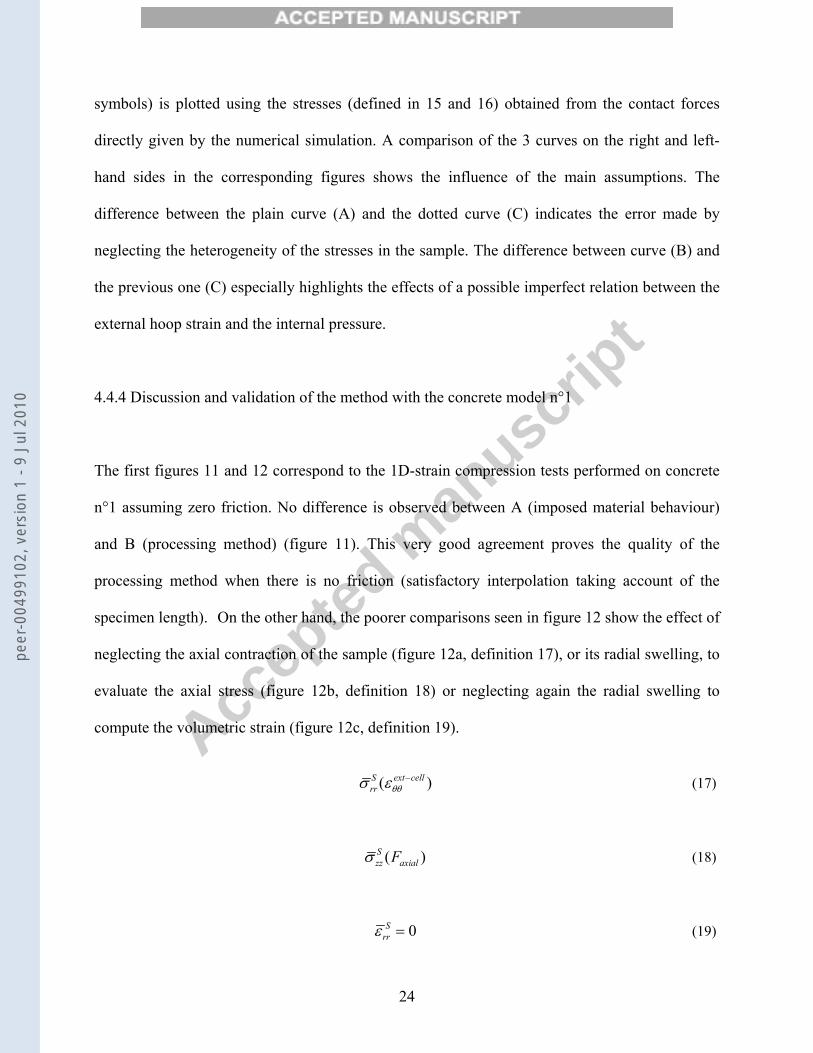
4.4.4 Discussion and validation of the method with the concrete model n°1
The first figures 11 and 12 correspond to the 1D-strain compression tests performed on concrete
n°1 assuming zero friction. No difference is observed between A (imposed material behaviour)
and B (processing method) (figure 11). This very good agreement proves the quality of the
processing method when there is no friction (satisfactory interpolation taking account of the
specimen length). On the other hand, the poorer comparisons seen in figure 12 show the effect of
neglecting the axial contraction of the sample (figure 12a, definition 17), or its radial swelling, to
evaluate the axial stress (figure 12b, definition 18) or neglecting again the radial swelling to
compute the volumetric strain (figure 12c, definition 19).
( )S ext cellrr θθσ ε − (17)
( )Szz axialFσ (18)
0Srrε = (19)
peer
-004
9910
2, v
ersi
on 1
- 9
Jul 2
010
Accep
ted m
anusc
ript
25
It would appear essential to take into account the plastic behaviour of the cell despite its
thickness. Indeed, with the assumption of purely elastic behaviour, one notes an important error
in the analysis of the deviatoric and hydrostatic behaviours when the inner pressure reaches
approximately 400 MPa. However, this pressure is largely exceeded in the tests presented later.
4.4.5 Influence of the concrete behaviour on the precision of the analysis
Figure 13 presents the analysis of the numerical simulations for types-2, 3 and 4 concretes. When
the compaction of the sample is more important (figures 13a and 13c) the analysis appears even
more precise. This is explained by the lower stresses and radial strains in the sample. One can
note that the method remains relevant up to an equivalent stress of 1000 MPa (figures 13b and
13c). The final bulk modulus, which is reached for a pressure higher than 1 GPa, is correctly
described (figure 13b). These 4 numerical simulations confirm that the method correctly predicts
the hydrostatic and deviatoric behaviours of geomaterials for a large range of volumetric strains
and hydrostatic pressures. The influence of friction on the quality of the analysis is discussed in
the following section.
4.4.6 Influence of the friction on the precision of the analysis
In the calculations leading to figure 14, a coefficient of friction equal to 0.1 was used at the
concrete sample/ring interface. The contact between the plug and the sample is assumed to be
frictionless. In the first case (figure 14a, concrete n°1), one observes a maximum difference (≈
9%) between curves A and B which is definitely more important than the case without friction
peer
-004
9910
2, v
ersi
on 1
- 9
Jul 2
010

Accep
ted m
anusc
ript
26
(figure 11). A significant difference (between 10% and 17%) is also observed between curves A
and C. This last comparison shows that the difference does not come from a poor estimation of
the radial stress but is rather due to the shear stresses induced by the friction. It is also seen that
the volumetric strain (from curves B or C) is underestimated at the end of the loading. Both
results are in very good agreement with the evaluation of the effects of the friction made in
subsections 4.3.3 (overestimation of the axial stress, equation 7) and 4.3.2 (increase of radial
strain). Finally, the observed difference between curves A and B (volumetric strain) is less than
about 5%, up to a pressure of 900 MPa (figure 14a).
Surprisingly, for the type-3 concrete, the deviatoric stress given by curve (B) is not over-
estimated compared to that calculated from curve (C). Once again, this is explained by the
calculations of subsection 4.3.3 (see equations 7 and 8 with σdev/P ≈ 1 and f = 0.1). Indeed, it is
shown that a friction coefficient equal to 0.1 leads to a relative over-estimation of the axial stress
close to 10% and to a relative over-estimation of the radial stress close to 4% (figure 6). When
the deviatoric stress increases with pressure with a ratio (σdev/P) close to one (as it is the case in
figure 14b), these two effects compensate very well and the deviation (comparing curve B to
curve A) in the analysis disappears in spite of the friction (see equations 9 and 10). It follows that
curve (B) is very close to curve (A) (figure 14b).
These calculations with friction (f = 0.1) were also performed in the case of type-2 and 4 concrete
models (corresponding to 20% compaction for a hydrostatic pressure of 1 GPa). One observes a
relative deviation smaller than that obtained with the concrete models 1 and 3 due to a lower
radial stress level.
These numerical simulations made it possible to evaluate the quality and the robustness of
the proposed processing method for 1D-strain compression tests. It appears necessary to take into
peer
-004
9910
2, v
ersi
on 1
- 9
Jul 2
010

Accep
ted m
anusc
ript
27
account the plastic strain of the confining cell when the inner pressure exceeds approximately
400 MPa. Moreover, as shown in the numerical simulations of the test, one also needs to take into
account the sample shortening and its small radial expansion. Friction has a limited influence
when the friction coefficient does not exceed 0.1. To conclude, according to these numerical
simulations, the deviation from real values of the deviatoric stress and of the volumetric strain
due to the method will remain less than 10% and 5%, respectively. According to the last
numerical simulation, the deviation of the deviatoric stress will not exceed a few percent if the
deviatoric stress increases with pressure with a ratio (σdev/P) close to one. This situation
corresponds to the concrete tested, the results of which are presented in the next section.
5. Dynamic behaviour of MB50 concrete
Three dynamic 1D-strain compression tests were carried out with MB50 concrete samples
(diameter: 30 mm, height: 40 mm) and with the confining cells described above. These samples
were loaded with the Split Hopkinson Pressure Bars described in section 3. The method used for
the analysis of the test results has been presented in section 4.3. The assumption of negligible
friction between the cell and the specimen was especially addressed. The deviatoric behaviour
(evolution of the deviatoric stress versus the hydrostatic pressure) and the hydrostatic behaviour
(evolution of the hydrostatic pressure versus volumetric strain) are computed. A comparison
between the 3 tests will allow for an evaluation of the strain-rate effect.
peer
-004
9910
2, v
ersi
on 1
- 9
Jul 2
010

Accep
ted m
anusc
ript
28
5.1 GENERAL FEATURES
As explained in section 3, SHPB data processing provides forces and displacements at the
bar ends. Checks were performed that the input and output forces were close enough to each
other to ensure the homogeneity of stress fields in the specimen. Equation 2b shows that the
output force is a direct measurement (directly proportional to the strain of the transmitted wave)
by contrast with the input force (proportional to the algebraic sum of waves with opposite signs).
This input force is therefore more affected by experimental noise. Confidence in the specimen
equilibrium having also been obtained by numerical simulations (not reported in the paper), the
axial force is, in the following, deduced from the output force only. This is in perfect agreement
with the traditional data processing of the SHPB [25]. The nominal axial strain-rate is directly
derived from formula 2a. Its evolution versus time basically depends on the stress-strain response
of the specimen, as is always the case with the SHPB. Having measured the variation of strain-
rate with time, the average strain rate is arbitrary defined, in what follows, as the mean value
between the time corresponding to the maximum strain rate (≈ 110 µs, figure 15a) and the end of
the test (≈ 870 µs, figure 15a). The strain versus time shown in figure 15a looks monotonic as the
result of integration.
The results of three tests are presented corresponding to three axial strain-rates: 80 s-1, 141
s-1, 221 s-1 (associated with striker speeds of 6.13, 12.5 and 19.23 m/s, respectively)
5.2. TEST ANALYSIS (special focus on test n°2)
Note that, in the case of tests n°1 and 3, the same figures as those presented later may be found in
peer
-004
9910
2, v
ersi
on 1
- 9
Jul 2
010

Accep
ted m
anusc
ript
29
appendix A, with particular comments when needed. A special focus on test n°2 is made. This
test corresponds to a 1D-strain compression test carried out at a mean strain rate equal to 141 s-1.
The velocity of the striker is equal to 12.5 m/s. The maximum strain rate reached during the test
is equal to 223 s-1.
5.2.1 Experimental data
The evolution of the hoop strains (figure 15b) shows that the strain level at gauge G2, middle of
specimen (z = 0 in figure 1b), is higher than at gauges G1 and G3 (z = ± 3H/8) which is in
agreement with calculations made in subsection 4.3 (figure 8).
The maximum hoop strain G2 is equal to 0.15%. Consequently, the cell does not have a purely
elastic behaviour (by contrast with test n°1 – see appendix A). Moreover, the strain recorded by
the G5 (axial, z = 0) gauge is negative during the first 100 µs. This axial strain evolution (εzz(z=0,
ext)) is in agreement with the simulations done without friction (f = 0) that are presented in section
4 (figure 7 for instance). When the shortening of the sample is small, the positive hoop strain due
to internal pressure induces a negative axial strain (by the Poisson’s ratio effect). The barrelling
of the cell which appears later with the shortening of the specimen induces a positive (tension)
axial strain.
5.2.2 Data processing using the proposed method
Looking at the average stress fields in the sample (figure 15c), two phases are observed. Between
0 and 200 µs, the axial stress increases whereas the radial stress remains very low, just as in a
peer
-004
9910
2, v
ersi
on 1
- 9
Jul 2
010

Accep
ted m
anusc
ript
30
uniaxial compression test. The deviatoric stress is then very close to the axial stress. Between 200
and 800 µs, the deviatoric stress increases slowly. The radial stress reaches 450 MPa at the end of
the loading while the hydrostatic pressure exceeds 640 MPa. The axial strain evolves from 0 to -
12% (figure 15d) and the inner radial strain remains negligible by comparison with the axial
strain (|εrrmax/εzz
max| = 3.4%). The test is thus proved to be a quasi-1D-strain compression test.
5.2.3 Hydrostatic and deviatoric behaviours
The deviatoric and the hydrostatic behaviours of this test are plotted in figure 16. The deviatoric
stress shows a change in the response for a pressure of the order of 100 MPa. The hydrostatic
behaviour is quasi-linear for a pressure greater than 100 MPa and has an apparent bulk modulus
around 6 GPa. Very close values are found in the three tests (figure 17).
The measured hydrostatic and deviatoric behaviours do not show strong differences with those
assumed for the KST model (particularly in the case of concrete model n°4 that compares figure
13c with figures 16 and 17). It confirms that the above numerical simulations are realistic.
5.3. DISCUSSION
5.3.1 Comparison of the deviatoric and the hydrostatic behaviours obtained for the 3 tests
The results obtained in the 3 tests are very close to each other (figure 17, left hand side). Indeed,
the corresponding curves are almost superimposed in the pressure range from 50 to 500 MPa.
This suggests that the strain rate has a weak influence on the deviatoric behaviour in the observed
peer
-004
9910
2, v
ersi
on 1
- 9
Jul 2
010

Accep
ted m
anusc
ript
31
domain.
In the same way, the curves describing the hydrostatic behaviour of the 3 tests are well
superimposed in the volumetric strain range from 0 to -11% (figure 17, right hand side). The
hydrostatic behaviour also seems weakly influenced by the strain rate in the observed range.
5.3.2 Comparison of the results given by test n°2 with those found in the literature
Figure 18 shows a comparison of the results of the 1D-strain test n°2 (141 s-1) with results found
in the literature for the same concrete (MB50): quasi-static 1D-strain tests performed by Gatuingt
[21] with a smaller cell (external diameter: 50 mm) allowed the hydrostatic (figure 18, right hand
side) and the deviatoric behaviours (figure 18, left hand side) [39] to be obtained. Despite the
small variations in properties of MB50 concrete, the purpose of the following comparison is not
to elaborate a precise concrete model. It is to reinforce the validation of the test and of the
processing method by showing that the results are not in contradiction with other results found in
the literature. MB50 concrete was also submitted to quasi-static tri-axial tests [23], the results of
which are also plotted in figure 18 (left hand side). During these tests, the specimen was first
loaded under a pure hydrostatic pressure and then submitted to an axial loading. Several loading
paths are shown in figure 18 (left hand side) ending with the maximum deviatoric stress which is
reached. The hydrostatic response to pure hydrostatic loading is shown in figure 18 (right hand
side).
The deviatoric behaviours are very similar in the intermediate range of pressure (300 MPa-600
MPa). In this range, the influence of the strain rate and of the loading path appears quite small.
For higher pressures, a difference appears: the dynamic test can lead to a higher deviatoric stress
(950 MPa, test n°3, 221 s-1, figure 17) than that of the triaxial test (550 MPa, figure 18)
peer
-004
9910
2, v
ersi
on 1
- 9
Jul 2
010

Accep
ted m
anusc
ript
32
performed with the highest pressure of confinement (800 MPa).
When quasi-static and 1-D strain tests are observed together, the hydrostatic behaviour of
concrete MB50 appears to be influenced by the loading rate. When quasi-static 1D-strain test and
the response under a pure hydrostatic loading are compared, it appears to significantly depend on
the loading path.
Conclusion
The three 1D-strain compression tests show that the deviatoric and hydrostatic behaviours
appear almost independent of the strain rate in the (rather narrow) studied range of strain rates
(80-221 s-1). The deviatoric strength increases monotonically with the hydrostatic pressure to
reach 950 MPa under a pressure of 900 MPa (test n°3).
This result is different from that obtained in triaxial quasi-static compression tests on the same
concrete (MB50), for which a maximum in the deviatoric resistance of around 550 MPa was
observed [23]. This difference can be attributed to a strain-rate effect (4 orders of magnitude
between quasi-static and the present tests) or it indicates a possible influence of the loading path
on the response.
Considering the hydrostatic behaviour, an almost constant dynamic bulk modulus (around 5 to
6 GPa) was observed with the three 1D-strain compression tests up to a pressure of 900 MPa.
This is smaller than that deduced from purely hydrostatic compression tests (9 to 20 GPa in that
case) using a tri-axial cell (same concrete) [23] but greater than that obtained with a quasi-static
1D-strain test (3 to 4 GPa in that case). The influence of the strain-rate for equivalent loading
paths (1D-strain) appears sizeable. However, the comparison between the two quasi-static tests
peer
-004
9910
2, v
ersi
on 1
- 9
Jul 2
010

Accep
ted m
anusc
ript
33
underlines once again the importance of the loading path.
New information is provided by the tests presented in this paper. The most important, at the
present stage, is the description of a new testing device giving 1D strain loading of geomaterials
in the dynamic range and the proposition of a method to efficiently analyse experimental data.
This method leads to the knowledge of the deviatoric and hydrostatic behaviours of the material
tested. It is shown that the plastic behaviour of the cell as well as the shortening and the swelling
of the specimen have to be taken into account in the analysis. The possible influence of a friction
coefficient (smaller than 0.1) between the specimen and the cell was investigated by means of
numerical simulations of the cell loaded by internal pressure and internal shear stress. Various
numerical simulations of the test were carried out with different sets of parameters for the
concrete plasticity model of Krieg, Swenson and Taylor. The method was applied successfully to
artificial experimental data (free of noise) provided by those simulations. Moreover, two
numerical simulations were performed with a constant friction coefficient equal to 0.1. These
proved there is a weak influence of friction (between the cell and the sample) on the computed
response of the concrete behaviour. This is especially true when the deviatoric resistance
monotonically increases with the hydrostatic pressure with a ratio close to one. In addition, two
methods of assessing the friction based on the outer strains ratio were also proposed and
discussed. These two methods were used in experiments showing the friction coefficient is closer
to 0 than to 0.1.
A high level of compaction strain (20%) can be produced with this testing device. It mostly
operates in a 1D-strain situation. Stresses up to 1000 MPa, confinement pressures up to 600 MPa
and a strain rate range between 100 and 500 s-1 can be achieved to provide suitable data to
evaluate the dynamic behaviour of concrete and other rock-like materials under multiaxial
dynamic loadings.
peer
-004
9910
2, v
ersi
on 1
- 9
Jul 2
010

Accep
ted m
anusc
ript
34
Appendix A
TEST N°1 (average strain rate: 80 s-1)
The striker velocity for this test was 6.13 m/s, leading to a maximum strain rate of 145 s-1 and to
an average strain rate of about 80 s-1. The external hoop-strains that were recorded on the cell are
presented in figure 19b. The maximum hoop strain G2 is 0.064%. Consequently and according to
the numerical simulations presented in subsection 4.3 (figure 4), the behaviour of the cell remains
in the elastic domain. The difference between the signals of gauges G1 and G3 could be due to a
slight relative global displacement between the specimen and the cell.
The average radial stress in the sample (figure 19c) and its average radial strain (figure 19d) are
deduced from the measured hoop strains. The axial stress is deduced from the output force and
corrected for the above computed radial strain. It is observed that the loading can be divided into
two phases: Between 0 and 200 µs, the axial stress increases and the radial stress remains very
low, like in a uniaxial compression test. The deviatoric stress is therefore very close to the axial
stress. Later, between 200 and 800 µs, the deviatoric stress increases slowly. The hydrostatic and
deviatoric behaviours corresponding to test n°1 are shown in figure 17 (curve “80 s-1”).
TEST N°3 (average strain rate: 221 s-1)
This test corresponds to a 1D-strain compression test carried out at a mean strain rate equal to
peer
-004
9910
2, v
ersi
on 1
- 9
Jul 2
010

Accep
ted m
anusc
ript
35
221 s-1. The striker velocity was 19.23 m/s. The strain rate reached a maximum value equal to
415 s-1. Experimental data are plotted in figures 20a and 20b.
The maximum hoop strain G2 was 0.2%. Consequently, the cell did not have a purely elastic
behaviour, according to the numerical simulations presented in the subsection 4.3. According to
figure 7 in section 4.3., the negative sign of the axial strain (G5 gauge, z = 0) at the beginning of
the test indicates that the friction coefficient was closer to 0 than to 0.1 The same conclusion is
deduced from the small value of the ratio ( ( 0, ) ( 0, )/z ext z extzz θθε ε= = < 0.25) observed when the axial
strain was equal to 15% (t = 600 µs).
It is observed that the loading can again be divided into two phases (figure 20c). Between 0 and
100 µs, the axial stress increases and the radial stress remains very low, as in a uniaxial
compression test. Between 100 and 800 µs, the deviatoric stress and the hydrostatic pressure
increase up to 1000 MPa and 900 MPa, respectively. The radial stress reaches 570 MPa at the end
of the test. The axial strain reaches a maximum value of –19%. The inner radial strain remains
very small. Consequently this test was close to a 1D-strain compression test. The hydrostatic and
deviatoric behaviours corresponding to test n°3 are shown in figure 17 (curve “221 s-1”).
The ratio of the outer hoop strains (εθθ(z=3H/8, ext)/εθθ
(z=0, ext), figure 21) was computed from the
experimental data shown in figure 20b. It should be emphasised that this ratio remains equal to
approximately 0.8 whereas the axial strain is lower than -0.1. This ratio can be compared with
that calculated by numerical simulation in the case of a cell subjected to an internal pressure
(figure 8, section 4.3). In the case of hpress = 34 mm, the computed ratio varied from 0.64 to 0.68,
depending on the internal pressure applied. The same ratio varied from 0.58 to 0.62 when an
internal shear loading corresponding to a friction coefficient equal to 0.1 was added. The value
peer
-004
9910
2, v
ersi
on 1
- 9
Jul 2
010

Accep
ted m
anusc
ript
36
found in the experiments (0.8) is closer to the result of the 1st numerical simulation (f = 0) than to
the result of the second simulation (f = 0.1). Thus, as explained in section 4.3, this ratio could be
used to compute an estimated value of the friction coefficient. In the present test, it indicates
again that the friction coefficient is closer to 0 than to 0.1.
peer
-004
9910
2, v
ersi
on 1
- 9
Jul 2
010

Accep
ted m
anusc
ript
37
References
[1] Burlion, N. Compaction des bétons : éléments de modélisation et caractérisation expérimentale.
PhD thesis. ENS Cachan, 1997. [2] Burlion N., Pijaudier-Cabot G. and Dahan N. Experimental analysis of compaction of concrete and
mortar. Int. J. Numer. Anal. Meth. Geomec 2001; 25:467-1486. [3] Le Vu O. Etude et modélisation du comportement du béton sous sollicitations de grande amplitude.
PhD thesis. Ecole Polytechnique, 1998. [4] Lindholm U. S., Yeakley L. M. and Nagy A. The dynamic strength and fracture properties of
Dressel basalt. International Journal of Rock Mechanical Mining Sciences and Geomechanical Abstract 1974; 11:181-199.
[5] Christensen R.J., Swansow S. R. and Brown W. S. Split Hopkinson bar test on rock under confining pressure. Experimental Mechanics 1972 ; 12:508-541.
[6] Klepaczko J. R., Gary G. and Barberis P. Behaviour of rock salt in uniaxial compression at medium and high strain rates. Archives of Mechanics, Warsawa 1991; pp.499-517.
[7] Goldsmith W., Polivka M., and Yang T. Dynamic behaviour of concrete, Experimental Mechanics, 1966; 6:65-79.
[8] Gong J.C., Malvern L.E. and Jenkins D.A. Dispersion investigation in the split Hopkinson pressure bar, Journal of Engineering Material Technology 1990; 112:309-314.
[9] Tang T., Malvern L.E. and Jenkins D.A., Rate effects in uniaxial dynamic compression of concrete, Journal of Engineering Mechanics 1992; 118:108-124.
[10] Gary G. and Klepaczko J. R. Essai de compression dynamique sur béton, GRECO Geomaterial scientific report, 1992, pp.105-118.
[11] Gary G. and Zhao H., Measurements of the dynamic behaviour of concrete under impact loading, In Chinese Journal Mechanics Press. Proceedings of 2nd ISIE'96. Beijing (China). 1996. p. 208-213.
[12] Malvern L.E., Jenkinds D.A., Tang T. and McLure S. Dynamic testing of laterally confined concrete, In: Micromechanics of failure of quasi brittle materials, Elsevier Applied Science, 1991, 343-352.
[13] Bertholf L.D., Karnes J. Two-dimensional analysis of the split Hopkinson pressure bar system, J. Mech. Phys. Solids 1975, 23:1-19.
[14] Davies E.D.H., Hunter S.C. The dynamic compression testing of solids by the method of the split Hopkinson pressure bar. J. Mech. Phys. Solids 1963, 11:155-179.
[15] Malinowski J. Z. and Klepaczko J. R. A unified analytic and numerical approach to specimen behaviour in split Hopkinson pressure bar system, Int J. Mech. Sci. 1986; 28: 381-391.
[16] Gorham, D.A. Specimen inertia in high strain-rate compression. J.Phys D Appl.Phys 1989; 22:1888-1893.
[17] Semblat J.F., Gary G. and Luong M.P., Dynamic response of sand using 3D Hopkinson bar, In: Proceedings of IS-TOKYO'95 First International Conference on Earthquake Geotechnical Engineering, Tokyo (Japan), 1995.
[18] Gary G., Bailly P., Behaviour of a quasi-brittle material at high strain rate. Experiment and modelling, European Journal of Mechanics 1998; 17(3):403-420.
[19] Bragov A.M., Grushevsky G.M. and Lomunov A.K., Use of the Kolsky Method for Studying Shear Resistance of Soils, Dymat Journal 1994; 3:253-259.
[20] Toutlemonde, F. Résistance au choc de structures en béton, PhD thesis, Ecole Nationale des Ponts et Chaussées, 1994.
[21] Gatuingt, F. Prévision de la rupture des ouvrages en béton sollicités en dynamique rapide, PhD
peer
-004
9910
2, v
ersi
on 1
- 9
Jul 2
010

Accep
ted m
anusc
ript
38
thesis, ENS Cachan, 1999. [22] Gatuingt F. and Pijaudier-Cabot G. Coupled damage and plasticity modelling in transient dynamic
analysis of concrete. Int. J. Numer. Anal. Meth. Geomec. 2002 ; 26 :1--24. [23] Buzaud, E. Performances mécaniques et balistiques du microbéton MB50. DGA/Centre d'Etudes de
Gramat report 1998. [24] Hopkinson B. A Method of measuring the pressure in the deformation of high explosive by impact
of bullets, Philosophical Transactions of the Royal Society of London 1914; A213:437-456. [25] Kolsky H. An investigation of mechanical properties of materials at very high rates of loading,
Proceedings of the Physical Society London 1949; B 62:676-700. [26] Achenbach, J.D. Wave propagation in elastic solids. Amsterdam. Elsevier Science Publisher. 1993. [27] Pochhammer L. Uber die fortpflanzungsgeschwindigkeiten kleiner schwingungen in einem
unbergrenzten isotropen kreiszylinder. J. für die Reine und Angewandte Mathematik 1876; 81:324-336.
[28] Chree, C. The equations of an isotropic elastic solid in polar and cylindrical coordinates, their solutions and applications. Trans. Cambridge Philos. Soc. 1889; 14: 250-369.
[29] Davies R.M. A critical study of the Hopkinson pressure bar. Phil. Trans. Of the Royal Soc 1948; A 240:375-457.
[30] Zhao H. and Gary G. On the use of SHPB technique to determine the dynamic behavior of the materials in the range of small strains, International Journal of Solids & Structures 1996; 33:3363-3375.
[31] Jahsman W.E. Re-examination of the Kolsky Technique for measuring dynamic Material behavior, J. Appl. Mech, 38. (1971): 77-82.
[32] Tyas A. and Watson A. J. An investigation of frequency domain dispersion correction of pressure signals, Int.J. Impact Eng. 2001; 25: 87-101.
[33] Gary G., Klepaczko J.R. and Zhao H. Corrections for wave dispersion and analysis of small strains with Split Hopkinson Bar, In: Proceedings of "International Symposium of Impact Engineering", Sendaï (Japan) 1992, 1:73-78.
[34] Hibitt H.D., Karlsson B.I., and Sorensen P. Abaqus User’s manuel, ABAQUS/IMPLICIT 6.1 2001. [35] Forquin P., Arias A., Zaera R. An experimental method of measuring the confined compression
strength of geomaterials. Int. J. Solids and Structures (Article in Press, Available on line) 2006. [36] Krieg R.D. A simple constitutive description for soils and crushable foams. Report, SC-DR-
7260883, Sandia National Laboratory 1978. [37] Swenson D.V. and Taylor L.M. A finite element model for the analysis of tailored pulse stimulation
of boreholes. Int. J. Num. Analyt. Meth. Geomech. 1983; 7:469-484. [38] Hibitt H.D., Karlsson B.I., and Sorensen P. Abaqus User’s manuel, ABAQUS/EXPLICIT 6.1 2001. [39] Forquin, P. Endommagement et fissuration de matériaux fragiles sous impact balistique, rôle de la
microstructure, PhD Thesis, ENS Cachan, 2003.
peer
-004
9910
2, v
ersi
on 1
- 9
Jul 2
010
Accep
ted m
anusc
ript
39
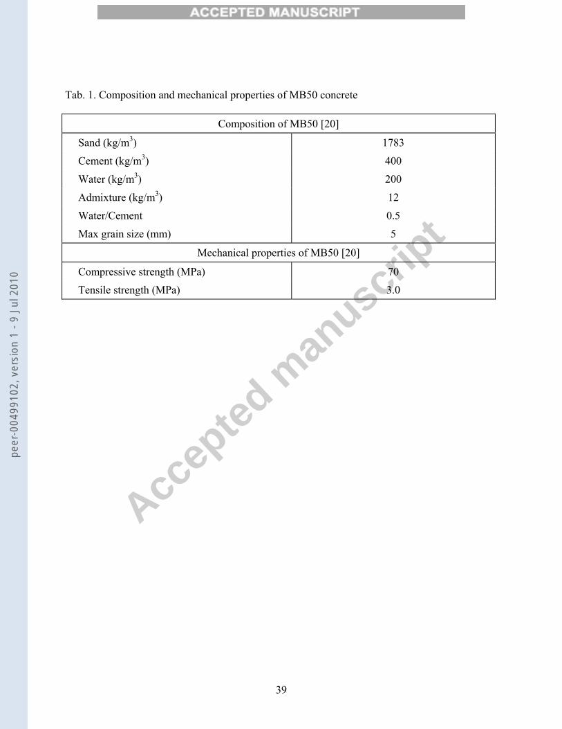
Tab. 1. Composition and mechanical properties of MB50 concrete
Composition of MB50 [20]
Sand (kg/m3) 1783
Cement (kg/m3) 400
Water (kg/m3) 200
Admixture (kg/m3) 12
Water/Cement 0.5
Max grain size (mm) 5
Mechanical properties of MB50 [20]
Compressive strength (MPa) 70
Tensile strength (MPa) 3.0
peer
-004
9910
2, v
ersi
on 1
- 9
Jul 2
010

Accep
ted m
anusc
ript
40
Tab. 2. Parameters of the Krieg, Swenson and Taylor model used in the numerical simulations
Density, Young’s modulus, Poisson’s ratio:
First point of the compaction curve:
Initial and final bulk moduli:
ρ, E, ν
εv(1), P(1)
Ki , Kf
2.386, 36 GPa, 0.2
-0.003, 60 MPa
20 GPa, 20 GPa
Coefficients of the elliptic equation: a0, a1, a2 1800 MPa2, 240 MPa, 0.6
4 sets of parameters used in the numerical simulations (cf. figure 9)
Concrete n°1:
Concrete n°2:
Concrete n°3:
Concrete n°4:
σmisesmax, εv
(2), P(2)
550 MPa, -0.1, 1 GPa
550 MPa, -0.2, 1 GPa
1000 MPa, -0.1, 1 GPa
1000 MPa, -0.2, 1 GPa
peer
-004
9910
2, v
ersi
on 1
- 9
Jul 2
010

Accep
ted m
anusc
ript
41
metallic ringconcrete cylinder
metallic compression plugs Fig.1a Fig.1b Position of the 6 gauges
Fig.1. Complete loading cell
G1 G2 G3
G4 G5 G6
3H/8 3H/8 H
peer
-004
9910
2, v
ersi
on 1
- 9
Jul 2
010

Accep
ted m
anusc
ript
42
Fig. 2. Basic waves recorded in test n°2 (striker speed: 12.5 m/s).
peer
-004
9910
2, v
ersi
on 1
- 9
Jul 2
010

Accep
ted m
anusc
ript
43
0
200
400
600
800
1000
1200
1400
0 0,02 0,04 0,06 0,08 0,1 0,12 0,14 0,16 0,18 0,2Plastic strain
Axi
al s
tres
s (M
Pa)
Test n°1
Test n°2
Identification
Fig. 3. 1D stress-strain behaviour of the steel of the cell
peer
-004
9910
2, v
ersi
on 1
- 9
Jul 2
010

Accep
ted m
anusc
ript
44
Fig. 4. Internal pressure versus external hoop strain, from the numerical simulation of a cell
internally loaded by a pressure applied to its central part (case A: 40 mm, case B: 34 mm)
peer
-004
9910
2, v
ersi
on 1
- 9
Jul 2
010

Accep
ted m
anusc
ript
45
Fig. 5. Internal hoop strains (z = 0 and z = h0 /2) versus external hoop strain (εθθ(z=0, ext)),
from the numerical simulation of a cell internally loaded by a pressure applied to its central part
(case A: 40 mm, case B: 34 mm)
peer
-004
9910
2, v
ersi
on 1
- 9
Jul 2
010

Accep
ted m
anusc
ript
46
Without shear loading:
With shear loading:
Fig. 6. Numerical simulation of a cell under internal pressure (0-800 MPa) and shear (0-80 MPa)
loading. Height of the loaded area: 40 mm
hpress /2
hpress /2
peer
-004
9910
2, v
ersi
on 1
- 9
Jul 2
010

Accep
ted m
anusc
ript
47
Fig. 7. Ratio of the external axial strain at middle point (z = 0) to the hoop strain at the same
point
peer
-004
9910
2, v
ersi
on 1
- 9
Jul 2
010

Accep
ted m
anusc
ript
48
Fig. 8. Ratio of hoop strain at point z = 3H/8 to the hoop strain at middle point (z = 0)
peer
-004
9910
2, v
ersi
on 1
- 9
Jul 2
010

Accep
ted m
anusc
ript
49
Fig. 9. Behaviour laws used for concretes n°1, 2, 3 and 4 (Left hand side: deviatoric strength
versus pressure, Right hand side: pressure versus volumetric strain)
peer
-004
9910
2, v
ersi
on 1
- 9
Jul 2
010
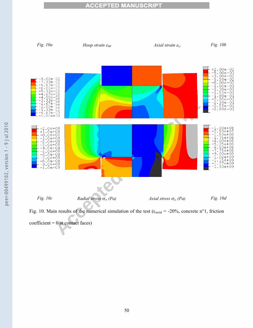
Accep
ted m
anusc
ript
50
Fig. 10a Hoop strain εθθ Axial strain εzz Fig. 10b
Fig. 10c Radial stress σrr (Pa) Axial stress σzz (Pa) Fig. 10d
Fig. 10. Main results of the numerical simulation of the test (εaxial = -20%, concrete n°1, friction
coefficient = 0 at contact faces)
peer
-004
9910
2, v
ersi
on 1
- 9
Jul 2
010

Accep
ted m
anusc
ript
51
Fig. 11. Results of the numerical simulation of the 1D-strain compression test (no friction
between the specimen and the cell, Concrete n°1)
peer
-004
9910
2, v
ersi
on 1
- 9
Jul 2
010

Accep
ted m
anusc
ript
52
Fig. 12. Illustration of possible uncompleted assumptions used in the processing of experimental
data (based on the results of the numerical simulation of the 1D-strain compression test - no
friction, concrete model n°1)
Fig. 12a, left. The shortening of the specimen is neglected to compute the radial stress
Fig. 12b, centre. The swelling of the specimen is neglected to compute the axial stress
Fig. 12c, right. The swelling of the specimen is neglected to compute the volumetric strain
peer
-004
9910
2, v
ersi
on 1
- 9
Jul 2
010

Accep
ted m
anusc
ript
53
Fig. 13a
Fig. 13b
Fig. 13c
Fig. 13. Results of numerical simulations of 1D-strain compression test
Fig. 13a. Concrete model n°2, no friction between the specimen and the cell
Fig. 13b. Concrete model n°3, no friction between the specimen and the cell
Fig. 13c. Concrete model n°4, no friction between the specimen and the cell
peer
-004
9910
2, v
ersi
on 1
- 9
Jul 2
010

Accep
ted m
anusc
ript
54
Fig. 14a
Fig. 14b
Fig. 14. Results of numerical simulations of 1D-strain compression test
Fig. 14a. Concrete model n°1, friction between the specimen and the cell: f = 0.1
Fig. 14b. Concrete model n°3, friction between the specimen and the cell: f = 0.1
peer
-004
9910
2, v
ersi
on 1
- 9
Jul 2
010
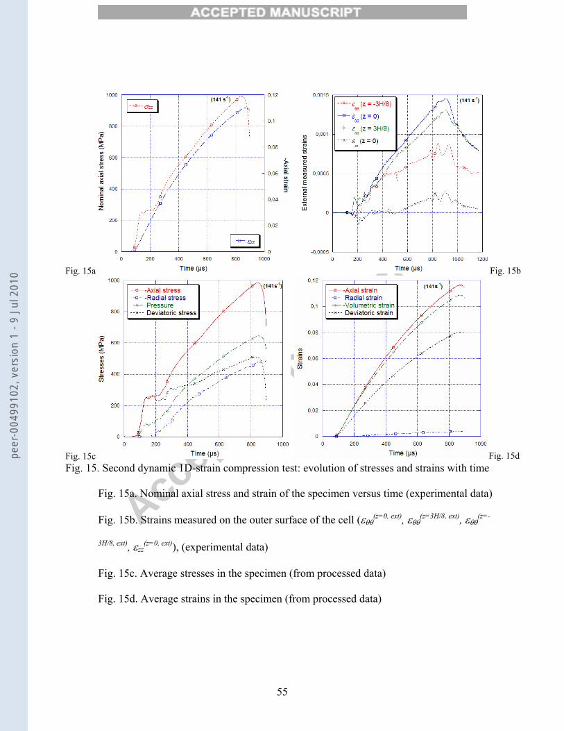
Accep
ted m
anusc
ript
55
Fig. 15a Fig. 15b
Fig. 15c Fig. 15dFig. 15. Second dynamic 1D-strain compression test: evolution of stresses and strains with time
Fig. 15a. Nominal axial stress and strain of the specimen versus time (experimental data)
Fig. 15b. Strains measured on the outer surface of the cell (εθθ(z=0, ext), εθθ
(z=3H/8, ext), εθθ(z=-
3H/8, ext), εzz(z=0, ext)), (experimental data)
Fig. 15c. Average stresses in the specimen (from processed data)
Fig. 15d. Average strains in the specimen (from processed data)
peer
-004
9910
2, v
ersi
on 1
- 9
Jul 2
010

Accep
ted m
anusc
ript
56
Fig. 16. Behaviours of concrete MB50 at strain rate of 141 s-1 compared with that of concrete
models n°1 and 4
peer
-004
9910
2, v
ersi
on 1
- 9
Jul 2
010

Accep
ted m
anusc
ript
57
Fig. 17. Comparison of the behaviour deduced from tests 1 to 3
peer
-004
9910
2, v
ersi
on 1
- 9
Jul 2
010

Accep
ted m
anusc
ript
58
Fig. 18. Comparison of behaviours of concrete MB50 based on measurements made with three
different experimental devices: 1D-strain test n°2; Quasi-static 1D-strain tests [21, 39]; Quasi-
static triaxial and purely hydrostatic compression tests (from Buzaud [23]).
peer
-004
9910
2, v
ersi
on 1
- 9
Jul 2
010

Accep
ted m
anusc
ript
59
Fig. 19a Fig. 19b
Fig. 19c Fig. 19dFig. 19. First dynamic 1D-strain compression test: evolution of stresses and strains with time
Fig. 19a. Nominal axial stress and strain of the specimen versus time (experimental data)
Fig. 19b. Strains measured on the outer surface of the cell (εθθ(z=0, ext), εθθ
(z=3H/8, ext), εθθ(z=-
3H/8, ext)), (experimental data)
Fig. 19c. Average stresses in the specimen (from processed data)
Fig. 19d. Average strains in the specimen (from processed data)
peer
-004
9910
2, v
ersi
on 1
- 9
Jul 2
010
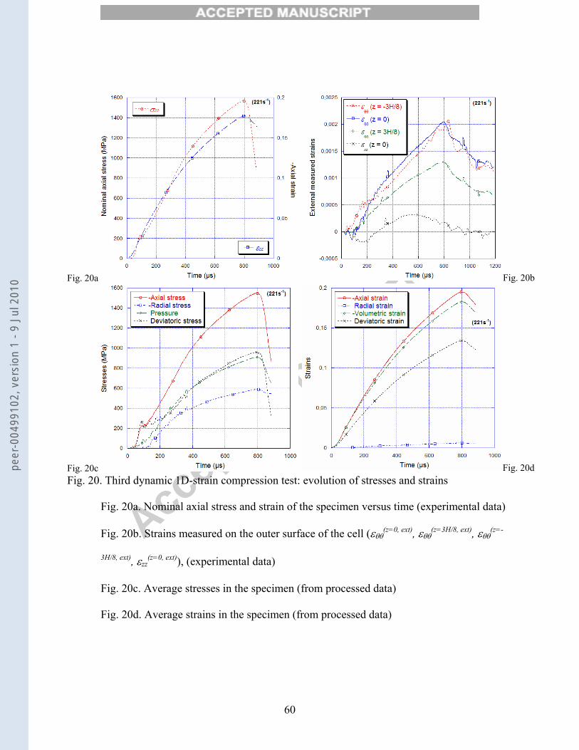
Accep
ted m
anusc
ript
60
Fig. 20a Fig. 20b
Fig. 20c Fig. 20dFig. 20. Third dynamic 1D-strain compression test: evolution of stresses and strains
Fig. 20a. Nominal axial stress and strain of the specimen versus time (experimental data)
Fig. 20b. Strains measured on the outer surface of the cell (εθθ(z=0, ext), εθθ
(z=3H/8, ext), εθθ(z=-
3H/8, ext), εzz(z=0, ext)), (experimental data)
Fig. 20c. Average stresses in the specimen (from processed data)
Fig. 20d. Average strains in the specimen (from processed data)
peer
-004
9910
2, v
ersi
on 1
- 9
Jul 2
010

Accep
ted m
anusc
ript
61
Fig. 21. Ratio of external hoop strains (εθθ
(z=3H/8, ext)/εθθ(z=0, ext))
peer
-004
9910
2, v
ersi
on 1
- 9
Jul 2
010