Embed Size (px)
Citation preview

A Theory of Demographic Transition and Fertility Rebound in the Process of Economic Development
Dimitrios Varvarigos, University of Leicester
Working Paper No. 13/19
September 2013

1
A Theory of Demographic Transition and Fertility Rebound in the Process of Economic Development
Dimitrios Varvarigos‡ University of Leicester
This Version: August 2013
Abstract Recent evidence of increasing fertility rates in developed countries, offers support to the idea that, from the onset of early industrialisation to the present day, the dynamics of fertility can be represented by an N-shaped curve. An OLG model with parental investment in human capital can account for these observed movements in fertility rates during the different phases of demographic change. A demographic transition with declining fertility emerges at the intermediate phase, when parents engage on a child quantity-quality trade-off. At later stages however, the continuing process of economic growth generates sufficient resources so that households can rear more children while still providing the desirable amount of educational investment per child.
Keywords: Demographic transition; Fertility rebound; Human capital
JEL Classification: J11, O41
‡ Address: Department of Economics, University of Leicester, Astley Clarke Building, University Road, Leicester LE1 7RH, United Kingdom. Telephone: ++44 (0) 116 252 2184. Email: [email protected].

2
1 Introduction
The analysis of the relation between economic development and demographic change has
received considerable attention over the last three decades. The prevailing approach seems
to favour the view that, since the onset of early industrialisation, population changes can be
categorised into two broad, but largely distinct, stages. During the first stage, fertility rates
and population growth increased drastically, while the second stage witnessed a demographic
transition for which one of the major characteristics is the striking decrease in fertility rates
(Galor 2005). Although the majority of existing theories have tended to focus mainly on the
second stage of the aforementioned changes (e.g., Galor and Weil 1996; Iyigun 2000;
Blackburn and Cipriani 2002; Bhattacharya and Chakraborty 2012; Varvarigos and Zakaria
2013), some seminal analyses have endeavoured to offer theoretical frameworks that account
for all the distinct phases of demographic change. For example, Becker et al. (1990)
constructed a theoretical model to show the existence of multiple development regimes in
which the low (high) income equilibrium corresponds to high (low) fertility rates. Tamura
(1996); Galor and Weil (2000); Lagerlöf (2003); and Strulik and Weisdorf (2008) have
provided more complete accounts of the circumstances under which an economy can
experience the transition from the early to the late stages of demo-economic outcomes.1
The process that commenced with the demographic transition, and continued during
most of the 20th century, led to a marked decline in fertility. In fact, some developed
countries experienced fertility rates that fell below replacement levels. To some extent,
demographers viewed this as a worrying trend, considering that the related outcome of
population ageing in these countries seemed to lay the foundations for a ‘trap’ in which the
low fertility rates could persist (Goldstein et al. 2009). This is because the fraction of the
population that belongs to their reproductive age declined as well, reinforcing the incidence
of low fertility rates – an outcome that could lead to far-reaching consequences for the
overall socio-economic environment of the countries that experienced such circumstances.
Nevertheless, more recent projections and empirical evidence are appeasing some of
these concerns. Many researchers now agree that developed economies are entering a new
phase of demographic change – a phase that is characterised by (once more) increasing
fertility rates. Alkema et al. (2011) constructed a Bayesian projection model that they used to 1 Tabata (2003) and Strulik (2008) also offer frameworks under which the dynamics of fertility can be traced along an inverted U-shaped curve.

3
forecast the trend in the Total Fertility Rate (TFR) for each country, up to the year 2100.
With few exceptions, their projections indicate that the phase of increasing fertility rates
among developed nations will most probably become a permanent characteristic during the
coming decades, thus indicating that the fertility rebound reflects a change in trend rather
than a mere temporary (or cyclical) change. A similar change in trend is suggested by Collins
and Richards (2013) who use quantitative population models in order to project the
evolution of fertility rates. In fact, recent empirical evidence suggests that the phase
characterising the fertility rebound can already be observed in developed countries. Myrskylä
et al. (2009) apply panel data estimation techniques for a sample of 37 countries from 1975 to
2005 and find that the relation between the Human Development Index (HDI) and the TFR
is U-shaped. Particularly, there is a threshold level for the HDI below which the relation
with the TFR is negative, whereas above it the relation with the TFR is positive. Despite the
fact that per capita GDP is a major component of the HDI, Luci and Théveron (2010)
argued that the results of Myrskylä et al. (2009) may not indicate the pure effect of economic
development on the observed fertility rebound. For this reason, they use a panel data set of
30 OECD countries over the period that spans from 1980 to 2007, in order to estimate the
effect of GDP per capita on the TFR. Their results, however, verify the idea that the decline
in fertility is halted and fertility rates start increasing at higher stages of economic
development, as they also find a U-shaped relation between the TFR and per capita GDP. It
is important to note that, in both the aforementioned analyses, the significance of this type
of non-monotonic effect is robust to adjustments in the TFR that are made to account for
the fact that the timing of childbearing may shift to later stages of the reproductive age – an
outcome that is conventionally used to account for subsequent reversals in fertility trends
(Lee 2003). Goldstein et al. (2009) argue that “the trend of increasing TFR has not been
limited to the countries with very low fertility, but took place across the developed world”
(page 670). Among the possible explanations for this phenomenon, they include the
improvement in economic conditions, such as the increase in GDP per capita. It is worth
noting that while conventional wisdom would attribute this effect to immigration, the
empirical analysis of Tromans et al. (2009) does not support this argument. Using the recent
increase of the TFR in the United Kingdom, they show that a large part of the increase in
the TFR is attributed to UK born women rather than foreign born ones, thus suggesting that
immigration is not the only factor behind the fertility rebound.

4
The aforementioned evidence on the fertility rebound in developed economies,
combined with the changes in fertility trends since the beginning of early industrialisation,
offers credence to the idea that the dynamics of fertility, along the various stages of
economic development, can be traced on an N-shaped curve. In the first stage, fertility rates
increase; the second stage witnesses a demographic transition, characterised by declining
fertility rates; and in the third stage, the trend is once more reversed as fertility rates are
increasing. The purpose of this paper is to offer a theory that accounts for such fertility
dynamics. Since the aforementioned evidence has shown that the ‘tempo’ effect and
immigration are not the only drivers of the recent fertility rebound in developed economies,
this theory will focus on the impact of increasing income that is associated with the
economy’s transition to higher stages of economic development.
I construct an overlapping generations model in which households care about both the
size of their family and the human capital of their children. Both child-rearing and the
parental investment on education entail costs that are measured in units of output. The
government collects taxes and uses them to finance the provision of public services, the
various effects of which can be manifested as either complements or substitutes to private
education investment. At low levels of development, households find optimal not to invest
any of their income towards their children’s education; therefore, a rise in disposable income
leads to an increase in the number of children raised. As the economy grows, there is a
critical level of development at which parents start investing in the education of each of their
children. The high return to educational investment, coupled with the relatively limited
resources at the disposal of each household, lead to a quantity-quality trade-off. Parental
investment in human capital occurs at the expense of family size; thus, fertility rates decline.
Nevertheless, as per capita income grows even further, families are not constrained by such
trade-offs. Instead, disposable income is high enough so that fertility rates increase, while
parents can still invest resources towards their children’s education.
With regard to the existing literature, this paper is related to the analyses that have
examined the joint determination of economic and demographic outcomes on the basis of
models that introduce choices for fertility and parental investment towards each child’s
education. In addition to the analyses that have already been mentioned, other influential
papers on this strand of literature are those by Kalemli-Ozcan (2002); Hazan and Berdugo
(2002); de la Croix and Doepke (2004, 2009); Moav (2005); and Galor and Mountford (2008)

5
among others.2 Contrary to these analyses, I consider the case where the total costs
associated with having children (i.e., both rearing and education) are measured in units of
output rather than units of time. This approach is justified by the fact that the direct
pecuniary costs of child rearing represent a considerable fraction of a household’s total
income. For instance, Lino (2012) estimates that for a family with two children, the direct
child-related expenditures (per each child) on items such as shelter, food, clothing, health
care, child care, education, entertainment and other personal items account for roughly 20%
of a household’s income. While it is not my intention to downgrade the importance of the
opportunity costs of raising a child (stemming from the time/effort devoted by parents),
these statistics are a testament to the significance of the direct expenses associated with
child-rearing. Therefore, their consideration certainly merits more attention, especially since
the majority of analyses in the economic growth-demography nexus have mainly focused on
the time costs of raising the household’s offspring. As it turns out, the focus on pecuniary
expenditures facilitates an otherwise standard model in generating a fertility rebound at
higher stages of economic development. This is because the process of economic growth
generates enough resources so that a household’s decision to invest in education need not
necessarily be associated with the need to raise fewer children.
The exposition of the remaining analysis is as follows. In Section 2, I provide a detailed
description of the basic economic set-up. Section 3 considers the household’s (lifetime)
utility maximisation problem. In Section 4, I analyse the dynamics of human capital
accumulation while Section 5 analyses the dynamics of fertility. Section 6 concludes.
2 The Economy
Time is discrete and indexed by t . The economy is populated by overlapping generations of
households that have a lifespan of two periods – childhood and adulthood. During childhood,
individuals are reared by their parents and receive education that determines the stock of
human capital, or effective labour, that will be available to them when they become adults.
During adulthood, they receive a salary by offering their labour to perfectly competitive
firms. These firms produce units of the economy’s consumption good by utilising effective
labour under a linear production technology. This technology implies that the wage per unit 2 For empirical evidence on the quantity-quality trade-off, see Black et al. (2005) and Becker et al. (2010) among others.

6
of effective labour is constant over time. Henceforth, I denote the (constant) wage by 0ω
and assume that labour income is subject to a tax rate (0,1)τ . Adult households decide
how to allocate their after-tax (disposable) income between consumption, child-rearing, and
education expenditures per child.
Consider a household that begins adulthood during period t and suppose that the
members of the household wish to bear tn children. Rearing each child entails a fixed cost
of 0q units of output. Furthermore, parents may wish to spend resources towards the
education of each of their offspring. Denoting the amount of education expenditures per
child by tx , we can write the household’s budget constraint as
(1 ) ( )t t t tc τ ωh n q x , (1)
where tc denotes consumption and th is the stock of human capital, i.e., the variable that
ultimately determines the amount of effective labour available to each household.
As noted earlier, parents can affect each child’s human capital by devoting resources
towards their education. Particularly, given that each parent devotes tx units of output per
child, human capital will be
1t t t th ιz λm x , (2)
where , 0ι λ . Shortly, we shall see that the terms tz and tm represent functions that
incorporate the effect of public spending towards activities that support human capital
accumulation and the efficiency of labour. The government devotes tg units of output
towards these activities, an amount financed by the collected tax revenues according to a
balanced budget rule. Denoting the population of adult households by tN , the
government’s budget can be formally written as
t t tg τωh N . (3)
In order to avoid the complication that arises from scale effects, I am going to assume that
the benefit of publicly provided services on human capital depends on the amount of public
spending per household. Particularly, it is assumed that ( / )t t tz Z g N and
( / )t t tm M g N such that ( ) 0z and ( ) 0M respectively. Henceforth, I will employ
the specific functional forms

7
η
t tt
t t
g gz Z q
N N
, (0,1)η , (4)
and
(1 )ε
t tt
t t
g gm M q
N N
, (0,1)ε , (5)
where (0,1)q is a parameter that determines the allocation of expenditures among
different types of public services. Substituting (3)-(5) in Equation (2), we can write the
dynamics of human capital according to
1η ε
t t t th φh ψh x , (6)
where ( )ηφ ι qτω and ( ) (1 )ε εψ λ τω q are composite parameter terms.
Note that the ideas embedded in (2), (4) and (5) allow us to consider the general case
where the overall impact of public services entails both complementary and substitute effects
to the private resources devoted towards human capital improvements. Such a scenario is
actually quite intuitive. Whereas services on public education can be thought as a reasonable
substitute for the resources that the private sector dedicates to the accumulation of human
capital, other forms of public infrastructure investment, such as public health, public
transport, law and order etc., can support private investment towards activities that improve
the efficiency of labour. My framework allows the manifestation of both possibilities
concerning the overall effect of public services.
At this point, it is worth commenting on the technical role of introducing productive
public spending in the model. As it must be evident from Equations (3)-(6), including public
services as an input to the education technology is a convenient device to generate dynamics
in the formation of human capital, i.e., a direct relation between th and 1th . However, the
same outcome is possible without the need to resort to the idea of productive public
spending. For instance, I could have assumed that the dynamics of human capital are derived
directly from Equation (6), a scenario for which the effect of th would capture
intergenerational externalities in the formation of human capital, in the same manner as in
the large majority of overlapping generations models with education – too numerous to
mention here but the reader may consult Chapter 5.2 of de la Croix and Michel (2002).
Furthermore, the presence of the parameter 0φ would allow some basic knowledge to be

8
available, even in the absence of parental investment in education. It goes without saying
that my subsequent results would remain intact.
Another issue that should be noted is that the specification of the human capital
technology in (6) will be consistent with a stationary solution for the human capital stock, as
I shall establish shortly. Nevertheless, this property of the model is not crucial for the
determination of my results. Later it will become clear that the dynamics of fertility remain
identical even if one sets 1ε in (6), thus creating the conditions that allow an ever
increasing stock of human capital and, consequently, growth in the long-run.
The lifetime utility of the household is given by
1ln( ) (1 ) ln( ) ln( )t t t t tu γ c γ β n θ n h , (7)
where (0,1)γ and , 0β θ are preference parameters. In addition to the utility accruing
from the consumption of goods, households enjoy utility by the children they bear and raise
over their lifetime. In this context however, children are not only valued per se but also in
terms of their human capital, i.e., households also enjoy greater felicity by more educated
children – an (imperfectly) altruistic motive that may capture the idea that parents care about
their children’s human capital because this improves their future prospects.3
3 The Household’s Problem
Households make their choices so as to maximise their lifetime utility in (7), subject to the
constraints in Equations (2) and (6). In order to solve this problem, we can substitute these
constraints in (7) and maximise with respect to tn and tx . The respective first order
conditions are given by
( ) (1 )( )
, 0(1 ) ( )
tt
t t t t
γ q x γ β θn
τ ωh n q x n
, (8)
and
(1 )
, 0(1 ) ( )
εt t
tη εt t t t t t
γn γ θψhx
τ ωh n q x φh ψh x
. (9)
3 Rewriting the second part of the utility function as 1(1 ) ( ) ln( ) ln( )t tγ β θ n θ h , we can see that the
formulation in (7) implies that the utility weight on the number of children each household gives birth to is higher than the utility weight attached to human capital per child. This assumption is essential for the existence of an equilibrium with an interior solution for tn . The same technical condition has been used by Moav (2005) and de la Croix and Doepke (2009) among others.

9
The expressions in (8) and (9) offer some familiar conditions according to which the
marginal benefit from each activity must be equal to the corresponding marginal cost – both
expressed in terms of utility. The marginal utility cost in both cases is associated with the loss
of consumption that results from the increase in the resources required to raise and educate
the household’s offspring. The marginal utility benefit stems from the idea that parents enjoy
raising children, as well as supporting their education.
We can express (8) as an equality and solve it to get
(1 )( )
( ) (1 )(1 )( )t t t
γ β θn q x τ ωh
γ γ β θ
. (10)
According to Equation (10), a household will dedicate a fixed fraction of disposable labour
income in order to finance the total costs associated with having children – costs that
include both rearing and education. This fraction corresponds to the relative weight attached
to the utility that parents enjoy from their offspring. Next, we can substitute (8) in (9) and
express the latter as an equality. Solving this, we get
(1 )(1 )
(1 )( )η εt
t tt
τ ωhγ θ φx h
γ γ β θ n ψ
. (11)
Equation (11) reveals that the amount of resources that parents spend for the education of
each child has two components. With regard to the first component, the fraction of
disposable income devoted for total education expenditures is associated with the relative
weight attached to the utility accruing from the number of children, when these are
measured in effective terms (i.e., augmented by each child’s human capital). Naturally, the
educational resources per child are negatively related to the total number of children raised
by the household. As for the second component, it reveals that the substitutability associated
with public services reduces the incentive to provide private resources towards each child’s
education, thus reducing the private spending on education per child. This effect is mitigated
by the fact that public services also entail complementary effects, meaning that higher public
spending may also tend to increase the return to private investment in education.
The system of equations in (10) and (11) can be solved simultaneously to yield the
solutions for private education expenditures per child and fertility. These solutions are given
by
1
( ) max 0, ( ) η εt t t
φx χ h θq θ β h
β ψ
, (12)

10
and
1
(1 )(1 )( )if 0
(1 )( )
( )
(1 )(1 )if 0
(1 )( )
tt
t t
ε ηt
tε ηt
τ ωhγ β θx
γ γ β θ q
n ν h
τ ωψhγ βx
γ γ β θ qψh φ
, (13)
respectively. These two results can facilitate us in analysing and understanding the dynamics
of demo-economic development. The following section will focus on the evolution of
human capital, whereas the dynamics of population growth will be formally analysed in a
subsequent part of the paper.
4 Economic Dynamics
A closer look at the result in (12) reveals that there are circumstances under which parents
may find optimal not to invest any resources towards the education of their offspring. The
underlying cause for this possibility lies on the fact that as long as 0 0ι φ , each child
will still be endowed with units of efficient labour, due to the presence of human capital-
enhancing public services, even though parents may not invest any private resources towards
their education. In order to keep the analysis consistent with the existing literature and the
empirical evidence on the matter, it is natural to focus attention to the case where the
decision not to invest in the children’s education materialises at low levels of economic
development. Henceforth, I will be assuming that the condition ε η holds. Given this,
when the stock of human capital is relatively low, the utility cost of foregone consumption
outweighs the utility benefit of educating the children and increasing their efficiency.
Nevertheless, when the stock of human capital is relatively high, the complementary effect
of public services becomes strong enough to guarantee that the return to private investment
in education is sufficiently high to compensate parents for the utility loss due to decreased
consumption. The main message from this discussion can be summarised in
Lemma 1. Assuming that ε η holds, there exists a threshold
1
( ) ε ηθ β φh
θψq
such that

11
0
( )
[ ( )( / ) ]/
t
t tη εt t
if h h
x χ h
θq θ β φ ψ h β if h h
. (14)
Proof. From Equation (12), we can see that ( ) 0χ h and 1( )( )( ) 0η ε
t t
ε η θ β φχ h h
βψ .
Therefore, 0tx if and only if th h . Furthermore, the non-negativity constraint implies
that 0tx th h . □
The outcome summarised in Lemma 1 allows us to combine Equations (6) and (14) in
order to write the dynamics of human capital as follows:
1
for
( )
( / )( ) for
ηt t
t tε ηt t t
φh h h
h F h
θ β ψqh φh h h
. (15)
Using (15), we can characterise the dynamics of human capital through
Proposition 1. Assume that (1 )/(1 )ε ηθ βψq φ
θ
holds. Then, for any 0 0h , the economy will
converge to an asymptotically stable steady state h , such that h h .
Proof. See the Appendix. □
The dynamics of human capital are illustrated in the phase diagram of Figure 1. The
return to human capital investment is high enough so that the economy will eventually
exceed the threshold that governs the households’ decision to devote private resources for
the education of their children. This outcome supports the formation of human capital and
leads to a (relatively) high steady state equilibrium h .
The proof to Proposition 1 (see the Appendix) also reveals the outcome that transpires
when the condition (1 )/(1 )ε ηθ βψq φ
θ
is not satisfied. In the case where

12
(1 )/(1 )ε ηθ βψq φ
θ
, it is h h and ( ) (0,1)F h η
. Consequently, h
will emerge as a
stable steady state, at least for some range on the domain of th . Given that this equilibrium
is associated with 0tx , whereas my purpose is to examine a scenario for which a
transition from 0tx to 0tx will occur, I rule out this possibility when I analyse the
dynamics of fertility in the following section.
5 Fertility Dynamics
The purpose of this section is to trace the dynamics of fertility along the process of
economic development. I shall begin the analysis by using the results in (13) in order to
examine how fertility varies with the stock of human capital. This analysis leads to
Lemma 2. Consider ( )t tn ν h . It is straightforward to establish that
i. When 0tx , then ( ) 0tν h ;
ii. When 0tx , then there exists
1
(1 )ˆε ηε η φ
hψq
such that
th 0
( )tF h
1th
1t th h
h h
h h
Figure 1. The dynamics of human capital

13
ˆ0
( )
ˆ0
t
t
t
for h h
ν h
for h h
.
Proof. See the Appendix. □
It will be useful to make a comparison between the threshold values h and h . This exercise
is undertaken in
Lemma 3. As long as (1 )
1ε η θ
θ β
holds, it is h h .
Proof. The condition h h implies
1 1
(1 ) ( )ε η ε ηε η φ θ β φ
qψ θqψ
which is indeed true for
(1 ) /( ) 1ε η θ θ β . □
Now, we can gather the previous results in order to understand the qualitative impact of the
human capital stock on fertility. This is summarised in
Proposition 2. Consider ( )t tn ν h . Then
0
ˆ( ) 0
ˆ0
t
t t
t
for h h
ν h for h h h
for h h
. (16)
Proof. It follows from Lemmas 2 and 3. □

14
My objective is to analyse an economy that goes through all the stages of the possible
demographic changes, as it converges to the long-run equilibrium that is characterised by h .
With this in mind, let us consider
Lemma 4. Assume that (1 )/(1 ) (1 )/(1 )
1
( )/(1 )
(1 ) ( )max ,
( )
ε ηε η ε η
η
ε η η
β ε η φ θ β φqψ
θ ε η θ
holds. Then
ˆh h .
Proof. See the Appendix. □
The results in Proposition 2 and Lemmas 3 and 4 allow us to understand the movements
in fertility, and therefore population growth, as the economy goes through different stages of
the development process towards its convergence to the stationary equilibrium. From these
results, it follows that for an initial stock of human capital that satisfies 0h h , the economy
will initially exceed the threshold indicated by h and will subsequently exceed the threshold
indicated by h as well. Let us define time periods T and T such that
0, ... 1
, ...t
h for t T
h
h for t T
, (17)
and
ˆ ˆ, ...
ˆ ˆ 1, ...
t
h for t T T
h
h for t T
, (18)
where it should be noted that T T holds by virtue of Proposition 1 and Lemma 3. Given
these, a formal characterisation of the dynamics of fertility is possible through
Proposition 3. There are three different stages of fertility dynamics. Fertility increases from 0t to
1t T , it declines from 1t T to ˆt T , and it increases again from ˆt T onwards.

15
Proof. It follows from Equations (16)-(18). □
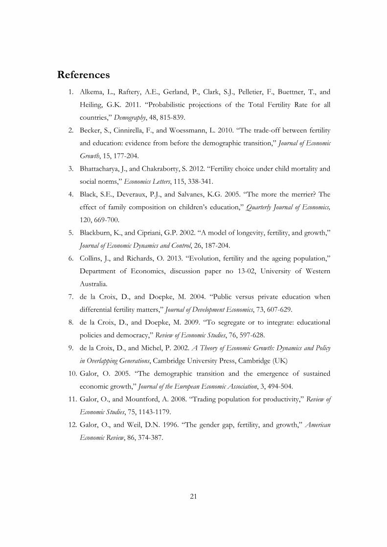
The dynamics of fertility/population growth are illustrated in Figure 2, where it is clear
that they depict an N-shaped graph. The intuition is the following. At the first stage
(corresponding to th h ), the return to the parental investment in education is so low that
parents decide to spend the amount of income that they do not consume, entirely for child-
rearing purposes. As disposable income grows, families have more resources so that they can
rear more children (see Equation 10 for 0tx , where child-rearing absorbs a constant
fraction of disposable income). Gradually however, the threshold defined by h will be
exceeded and the return to private education spending will be high enough to motivate
households to dedicate part of their resources towards this purpose. A better explanation of
the outcomes that transpire from this point onwards is possible if we use (13) and (14) to
write child-rearing and total education expenditures as fractions of disposable income. That
is
(1 )
( )(1 ) (1 )( )
ε ηt t
tε ηt t
qn qψhγ βδ h
τ ωh γ γ β θ qψh φ
, (19)
and
(1 )( )
( )(1 ) (1 )( )
ε ηt
t ttε η
t t
θqψh φ
β θn x γ β θζ h
τ ωh γ γ β θ qψh φ
, (20)
from where we can easily check that ( ) (0,1)tδ h and ( ) (0,1)tζ h for th h . From (19)
and (20), it follows that ( ) 0tδ h and ( ) 0tζ h , i.e., as the economy develops, parents
devote a decreasing fraction of their income towards child-rearing and an increasing part of
their income towards the education of their offspring. In fact, the return to education
spending is so high during the second stage (corresponding to ˆth h h ) that we observe
what is effectively a quantity-quality trade-off. In other words, households actually reduce
the number of children they rear in order to finance the optimal amount of education
expenditures per child. Nevertheless, the economy continues to grow and eventually reaches
the third stage (corresponding to ˆth h ). Now, disposable income is sufficiently high so that
a quantity-quality trade-off is not necessary. In other words, the share of total income on

16
child-rearing may be declining, but the increase in income is so pronounced that the overall
amount available for raising children is higher. Households have enough resources to raise
more children and still provide the desirable amount of education spending for each of
them, as the economy converges to its long-run equilibrium.
Despite the fact that I employ an education technology that results in a stationary
solution for human capital (see Proposition 1), the qualitative results of the model remain
intact even under a different specification that permits long-run growth. For instance, setting
1ε in (6) will alter the dynamics of human capital in the sense that, once in exceeds the
threshold defined by h , the economy will be able to sustain an equilibrium where the human
capital stock grows without bound. This would be the only qualitative change of the model’s
equilibrium behaviour though. The interested reader can use 1ε in Lemmas 1-4 and
Propositions 2-3 to verify that the results concerning the equilibrium characteristics of tx
and tn , as well as the dynamics of fertility, remain qualitatively identical. Therefore, the
fertility rebound at later stages of economic development is not a result that should be
attributed to the stationarity of human capital and GDP per capita since the same result
emerges under a set-up that allows growth in the long-run.
t 0
tn
T 1T
Figure 2. The evolution of the fertility rate

17
6 Conclusion
Recent empirical evidence suggests that those countries that have witnessed marked
reductions in their fertility since the onset of demographic transition, now appear to
experience a ‘fertility rebound’ with rising fertility rates. Among the various explanations for
this reversal, empirical evidence suggests that economic development – in the past, the main
engine behind the demographic transition – is now one of the driving forces behind this new
phase of demographic change.
This new evidence indicates that, from the beginning of early industrialisation to the
present day, the dynamics of fertility can be traced along an N-shaped curve. In this paper, I
presented a theory that accounts for this dynamic behaviour. The main theme of the analysis
is that the child quantity-quality trade-off – one of the main explanations for the
demographic transition in the economics literature – materialises in an intermediate phase
where the joint effects of the high return to human capital investment and the income
constraint faced by households, implies that parents can increase the investment towards
their children’s education, only at the expense of the number of children they bear over their
reproductive age. As incomes grow even further though, there is a new phase where parents
can provide the desirable expenditures towards the education of their offspring without
necessarily reducing the number of children they give birth to.
As it became evident from the main part of the paper, the model that underlines my
theory is qualitative rather than quantitative. Furthermore, it was constructed with the
purpose of offering analytical solutions that pinpoint the main mechanisms that characterise
the equilibrium outcomes without blurring their intuition. Naturally, a more general
framework that will be simulated numerically can be a fruitful avenue for future research.
Nevertheless, even in this simple form, my model is able to draw attention to an outcome
that, although is supported by recent evidence in demographic research, it has so far evaded
the attention of the literature on the nexus between economic growth and the demography.
As a final note, I should emphasise that my theory formalises just one of a variety of
possible explanations behind the fertility rebound in developed economies – the outcome
that is ultimately responsible for the emergence of N-shaped fertility dynamics. This should
not be viewed as a stance against other legitimate explanations for this phenomenon (e.g.,
the ‘tempo’ effect; immigration etc). These may offer important accounts behind the reversal

18
of fertility trends in developed countries; therefore their exploration certainly merits formal
analysis through future research work. In any case however, existing evidence (cited in the
Introduction) reveals that the ‘tempo’ effect and immigration cannot fully account for the
change in fertility trends in developed countries. Therefore, offering an additional or
complementary explanation was an endeavour certainly worth undertaking.
Appendix
Proof of Proposition 1
Consider the case where th h . According to (15), we have ( ) ηt tF h φh where
1( ) 0ηt tF h ηφh , (0)F and 2( ) ( 1) 0η
t tF h η ηφh . Furthermore, note that
11η ηh φh h φ
. However, it is true that h h
given that (1 )/(1 )ε ηθ βψq φ
θ
holds by
assumption. Consequently ( )t tF h h th h , meaning that the economy will not reach
the steady state h
because the dynamic behaviour of human capital will change when its
stock exceeds h . According to (15), the transition equation becomes ( ) ( )ε ηt t t
θF h ψqh φh
β
thereafter. Note that, by the definition of h
1
( ) ε ηθ β φh
θψq
( )ε ηθψqh θ β φ
ε ηθ θ βψqh φh
β β
1ε η ηθ θ βψqh φh φh
β β
( )ε η ηθψqh φh φh
β
lim ( ) lim ( )t t
t th h h h
F h F h
.
It is,

19
1 1( ) ( )ε ηt t t
θF h εψqh ηφh
β , (A1)
so that ( ) 0tF h as long as
1 1ε ηt tεψqh ηφh
ε ηt
ηφh
εψq
1ε η
t
ηφh h
εψq
,
which is true because h h
for ε η . Furthermore, given , (0,1)η ε , Equation (A1) reveals
that ( ) 0F . Therefore, for th h , the transition graph will cross the 045 line at a point
h , such that ( )h F h and
for
( )
for
t t
t
t t
h h h h
F h
h h h
.
It follows that ( ) (0,1)F h , allowing us to conclude that the fixed point h corresponds to
a stable equilibrium. □
Proof of Lemma 2
The first part of Lemma 2 is easily proven after using (13) for 0tx , and showing that
(1 )( ) (1 )( ) 0
(1 )( )t
γ β θ τ ων h
γ γ β θ q
. Next, we can consider the expression for fertility that
corresponds to 0tx . First of all, notice that the denominator ε ηtqψh φ is positive for
th h . Calculating the derivative, we get
1 1
2
(1 ) ( ) ( )(1 )( ) (1 )
(1 )( ) ( )
ε η ε η ε η ε ηt t t t
t ε ηt
ε η h qψh φ h ε η qψhγ βν h τ ωψ
γ γ β θ qψh φ
.
Obviously, the sign of the derivative will depend on the sign of the expression inside squared
brackets. In particular, it will be ( ) 0tν h as long as
1 1(1 ) ( ) ( ) 0ε η ε η ε η ε ηt t t tε η h qψh φ h ε η qψh

20
2( ) 2( )(1 ) (1 ) ( ) 0ε η ε η ε ηt t tε η h qψ ε η φh ε η h qψ
2( ) (1 ) 0ε η ε ηt th qψ ε η φh
[ (1 ) ] 0ε η ε ηt th h qψ ε η φ
1
(1 ) ˆε η
t
ε η φh h
qψ
.
Therefore, for ˆth h it is ( ) 0tν h . □
Proof of Lemma 4
Given ( )F h h and ( )t tF h h for th h , it is sufficient to show that ˆ ˆ( )F h h . This
condition corresponds to
ˆ ˆ ˆ( )ε ηθψqh φh h
β
1ˆ ˆ( )ε η ηθψqh φ h
β
1ˆ ˆε η ηβψqh φ h
θ
1
(1 ) (1 )η
ε ηε η φ β ε η φψq φ
qψ θ qψ
1
(1 )( )
η
ε ηβ ε η φε η φ
θ qψ
(1 )/(1 )
1
( )/(1 )
(1 )
( )
ε ηε η
η
ε η η
β ε η φqψ
θ ε η
.
Together with the fact that (1 )/(1 )( ) ε ηθ β φ
qψθ
holds by virtue of Proposition 1, then
(1 )/(1 ) (1 )/(1 )1
( )/(1 )
(1 ) ( )max ,
( )
ε ηε η ε η
η
ε η η
β ε η φ θ β φqψ
θ ε η θ
is sufficient to establish that ˆh h .
□
21
References
1. Alkema, L., Raftery, A.E., Gerland, P., Clark, S.J., Pelletier, F., Buettner, T., and
Heiling, G.K. 2011. “Probabilistic projections of the Total Fertility Rate for all
countries,” Demography, 48, 815-839.
2. Becker, S., Cinnirella, F., and Woessmann, L. 2010. “The trade-off between fertility
and education: evidence from before the demographic transition,” Journal of Economic
Growth, 15, 177-204.
3. Bhattacharya, J., and Chakraborty, S. 2012. “Fertility choice under child mortality and
social norms,” Economics Letters, 115, 338-341.
4. Black, S.E., Deveraux, P.J., and Salvanes, K.G. 2005. “The more the merrier? The
effect of family composition on children’s education,” Quarterly Journal of Economics,
120, 669-700.
5. Blackburn, K., and Cipriani, G.P. 2002. “A model of longevity, fertility, and growth,”
Journal of Economic Dynamics and Control, 26, 187-204.
6. Collins, J., and Richards, O. 2013. “Evolution, fertility and the ageing population,”
Department of Economics, discussion paper no 13-02, University of Western
Australia.
7. de la Croix, D., and Doepke, M. 2004. “Public versus private education when
differential fertility matters,” Journal of Development Economics, 73, 607-629.
8. de la Croix, D., and Doepke, M. 2009. “To segregate or to integrate: educational
policies and democracy,” Review of Economic Studies, 76, 597-628.
9. de la Croix, D., and Michel, P. 2002. A Theory of Economic Growth: Dynamics and Policy
in Overlapping Generations, Cambridge University Press, Cambridge (UK)
10. Galor, O. 2005. “The demographic transition and the emergence of sustained
economic growth,” Journal of the European Economic Association, 3, 494-504.
11. Galor, O., and Mountford, A. 2008. “Trading population for productivity,” Review of
Economic Studies, 75, 1143-1179.
12. Galor, O., and Weil, D.N. 1996. “The gender gap, fertility, and growth,” American
Economic Review, 86, 374-387.

22
13. Galor, O., and Weil, D.N. 2000. “Population, technology, and growth: from
Malthusian stagnation to demographic transition and beyond,” American Economic
Review, 90, 806-828.
14. Goldstein, J.R., Sobotka, T., and Jasilioniene, A. 2009. “The end of ‘lowest-low’
fertility?,” Population and Development Review, 15, 663-699.
15. Hazan, M., and Berdugo, B. 2002. “Child labour, fertility, and economic growth,”
Economic Journal, 112, 810-828.
16. Iyigun, M.F. 2000. “Timing of childbearing and economic growth,” Journal of
Development Economics, 61, 255-269.
17. Kalemli-Ozcan, S. 2002. “Does the mortality decline promote economic growth?,”
Journal of Economic Growth, 7, 411-439.
18. Lagerlöf, N.P. 2003. “From Malthus to modern growth: can epidemics explain the
three regimes?,” International Economic Review, 44, 755-777.
19. Lee, R. “The demographic transition: three centuries of fundamental change,” Journal
of Economic Perspectives, 17, 167-190.
20. Lino, M. 2012. “Expenditures on children by families, 2011,” U.S. Department of
Agriculture, Centre for Nutrition Policy and Promotion report no. 1528-2011.
21. Luci, A., and Théveron, O. 2010. “Does economic development drive the fertility
rebound in OECD countries?,” Institut National d'Études Démographiques (INED)
working paper no. 167.
22. Moav, O. 2005. “Cheap children and the persistence of poverty,” Economic Journal,
115, 88-110.
23. Myrskylä, M., Kohler, H.P., and Billari, F. 2009. “Advances in development reverse
fertility rates,” Nature, 460, 741-743.
24. Strulik, H. 2008. “Geography, health, and the pace of demo-economic
development,” Journal of Development Economics, 86, 61-75.
25. Strulik, H., and Weisdorf, J.L. 2008. “Population, food, and knowledge: a simple
unified growth theory,” Journal of Economic Growth, 13, 195-216.
26. Tabata, K. 2003. “Inverted U-shaped fertility dynamics, the poverty trap and
growth,” Economics Letters, 81, 241-248.
27. Tamura, R. 1996. “From decay to growth: a demographic transition to economic
growth,” Journal of Economic Dynamics and Control, 20, 1237-1261.

23
28. Tromans, N., Natamba, E., and Jefferies, J. 2009. “Have the women born outside the
UK driven the rise in UK births since 2001?” Population Trends, 136, 28-42.
29. Varvarigos, D., and Zakaria, I.Z. 2013. “Endogenous fertility in a growth model with
public and private health expenditures,” Journal of Population Economics, 26, 67-85.