A THEORY OF SURPLUS LABOUR

Kaushik Basu

Delhi School of Economics Delhi - 110 007

India

CONTENTS

1. The Problem

2. Basic Concepts

3. A Simple Model: The Casual Labour Market

3.1 Partial Equilibrium 3.2 General Equilibrium

3.3 Surplus Labou

r 4. Some Policy Issues

5. A Generalized Model 6.

Conclusion

1.

1. THE PROBLEM

Broadly speaking, an economy is said to have surplus labour or

disguised unemployment if it is possible to remove a part of its employed

labour force without causing a fall in aggregate output. The subject of

surplus labour once held the centre-stage of debates on subsistence

economies and agrarian structure and had generated an enormous literature.

However, the theoretical basis of these models was increasingly called into

question and interest in the subject faded out. Indeed, a closer

examination of these early works shows that explanations of surplus labour

were often based on either an unwitting use of irrational behaviour on the

part of agents or the use of very special assumptions concerning

preferences or technology.

This paper revisits this old subject in the belief that we can

rigorously define and explain surplus labour by drawing on recent advances

in the theory of efficiency wage, as exemplified by the works of Mirrlees

(1975), Rodgers (1975), Stiglitz (1976), Bliss and Stem (1978), and

Dasgupta and Ray (1986). I am referring here to the class of

efficiency-wage models which originate from Leibenstein's (1957, 1958) work

2 and shall refer to these writings as the efficiency-wage literature. The

basic axiom used in this literature is that in low-income economies there

exists a positive relation between the wages received by labourers and

their productivity.

The suggestion that this basic axiom can explain surplus labour is

not new. It was, in fact, an important motivation for Leibenstein's

original exploration (see also Mazumdar, 1959; Wonnacott, 1962). However,

as the efficiency-wage literature advanced, it became clear that the basic

2.

axiom cannot explain surplus labour or disguised unemployment within the

context of these models. It may be true that the withdrawal of a part; of

the labour force causes wages to rise and this in turn would cause the

remaining labourers to be more productive. But it is very easy to show (see

section 5 below) that in the existing models (e.g., Mirrlees, 1975) this

increased productivity can never be enough to fully compensate for the

3 withdrawn labourers,3 what the efficiency wage literature can explain well

is open unemployment and recent focus has been in that direction (Dasgupta

and Ray, 1986).

It will be argued in this paper that the basic axiom does indeed

4 provide a basis for surplus labour. The efficiency wage literature fails

to explain surplus labour because whenever it uses the basic axiom it uses

it in conjunction with another assumption, to wit, that the positive

relation between wage and labour productivity is perceived fully by each

employer. I shall refer to this as the perception axiom.

It will be argued in this paper that the two axioms are independent

and there are situations where, even though the basic axiom is valid, the

perception axiom is untenable. To understand this it is important to

recognise that there is a time-lag, often quite long, between wages and

productivity (see Bliss and Stem, 1978; Dasgupta and Ray, 1987; Osmani,

1987). Hence, in markets where landlords face a high labour turnover there

may be little relation between the wage paid by a particular landlord and

the productivity of his workers even though the basic axiom may be valid at

the aggregate level, that is, between the equilibrium market wage and

average productivity of labourers. The extreme example is provided by the

casual labour market where labourers are hired afresh each day. I shall

assume that the casual labour market is one where there is no relation

3.

between wage and productivity at the level of each landlord and model this

in section 3. Not only does this provide an analytically convenient polar

case, but the widespread existence of casual labour markets in reality (see

7 Binswanger and Rosenzweig, 1984; and Dreze and Mukherjee, 1987) makes this

model of some practical interest.

The polar case provides a plausible and theoretically consistent

explanation of surplus labour, raises some interesting policy issues

(section 4) and demonstrates the importance of modelling the case that has

been ignored in the literature, where the basic axiom is valid but the

perception axiom is not.

What happens in between the two polar cases of the efficiency-wage

literature and the model of section 3, that is, where the wage-productivity

link is not totally absent at the micro-level but neither is it fully

captured as required by the perception axiom? This is explored in section

5. It is shown that in this case both open and disguised unemployment can

be explained. Clearly, the exaggerated view of the non-existence of

disguised unemployment originated from the fact that the entire

efficiency-wage literature considers the polar case, which is also the only

case, where disguised unemployment cannot occur.

In the theory that is constructed in this paper, though the basic

axiom is true, each employer may have little or no incentive in resisting

wage cuts. This is consistent with experience (Rudra, 1982; Dreze and

Mukherjee, 1987) and suggests that for explaining rigidities we may have to

turn to labourers' preference and behaviour, rather than those of

employers.

2. BASIC CONCEPTS 4.

In this paper we need to distinguish between 'efficiency units' of

labour, hours of labour and labourers. Efficiency units capture the idea

of labour productivity. Production depends on the number of efficiency

units of labour used. The number of efficiency units that emerge from each

hour of labour depends on the wage rate (per hour), w, that the labourer

9

h = h(w), h'(w) ̂ 0 (1)

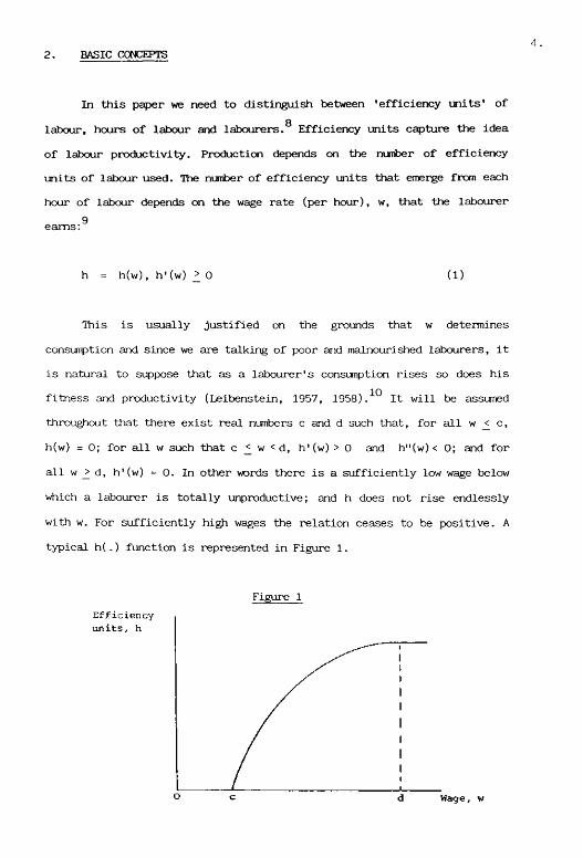
This is usually justified on the grounds that w determines

consumption and since we are talking of poor and malnourished labourers, it

is natural to suppose that as a labourer's consumption rises so does his

fitness and productivity (Leibenstein, 1957, 1958). It will be assumed

throughout that there exist real numbers c and d such that, for all w < c,

h(w) = 0; for all w such that c < w < d, h'(w) > 0 and h"(w)< 0; and for

all w > d, h'(w) = 0. In other words there is a sufficiently low wage below

which a labourer is totally unproductive; and h does not rise endlessly

with w. For sufficiently high wages the relation ceases to be positive. A

typical h(.) function is represented in Figure 1.

Figure 1

5.

The output produced on a landlord's farm depends on the number of

efficiency units of labour that is employed. If n hours of labour is

employed and each hour of labour produces h efficiency units, then output,

x, is given by:

x = x(nh), x' > 0, x" < 0 (2)

It will be assumed that, for all real number r for which x'(r) > 0, it must

be the case that x"(r) <0.

6.

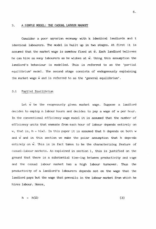
3. A SIMPLE MODEL: THE CASUAL LABOUR MARKET

Consider a poor agrarian economy with k identical landlords and t

identical labourers. The model is built up in two stages. At first it is

assumed that the market wage is somehow fixed at w. Each landlord believes

he can hire as many labourers as he wishes at w. Using this assumption the

landlord's behaviour is modelled. This is referred to as the 'partial

equilibrium' model. The second stage consists of endogenously explaining

the market wage w and is referred to as the 'general equilibrium'.

3.1 Partial Equilibrium

Let w be the exogenously given market wage. Suppose a landlord

decides to employ n labour hours and decides to pay a wage of w per hour.

In the conventional efficiency wage model it is assumed that the number of

efficiency units that emanate from each hour of labour depends entirely on

w, that is, h = h(w). In this paper it is assumed that h depends on both w

and w and in this section we make the polar assumption that h depends

entirely on w. This is in fact taken to be the characterizing feature of

casual-labour markets. As explained in section 1, this is justified on the

ground that there is a substantial time-lag between productivity and wage

and the casual labour market has a high labour turnover. Thus the

productivity of a landlord's labourers depends not on the wage that the

landlord pays but the wage that prevails in the labour market from which he

hires labour. Hence,

h = h(w) (3)

7.

Assuming that the price of the good is unity, the landlord's profit,

R, is given by:

R(n,w) = x(nh(w)) - nw (4)

If the landlord pays a wage below w, no labour will come to him. So his aim

is to maximize R(n,w) subject to w > w.

It is easy to see that the landlord would like to pay as low a wage

as possible. Hence, he sets wage equal to w. Having done so, he chooses n

to maximise R(n, w). Clearly the value of n depends on w. So we write

n = n(w) (5)

Since n(w) maximizes R(n,w), hence, using the first-order condition, we

know:

x'(n(w)h(w)) = w (6) hlw)

Given (5) we can compute the aggregate employment in the economy by

simply multiplying n(w) by k. This completes our description of the partial

equilibrium. If the wage prevailing in the labour market is w, then each

landlord pays a wage of w and hires n(w) hours of labour, where n(w) is

defined implicitly by (6). Our next task is to enquire into the

determination of w.

3,

3.2 General Equilibrium

In section 3.1 we learned to compute the total demand for labour,

given an exogenous w. If we do this experiment for different values of w,

what we end up deriving is the aggregate demand function for labour:

D = kn(w), (7)

where D is the total demand for labour.

To derive the equilibrium market wage, w, all we have to do is to

specify the aggregate supply curve of labour and then find the wage at

which demand equals supply. Before going on to such an exercise, let us

analyse the shape of the demand curve. The basic axiom renders the shape

unusual and our subsequent theorems require us to appreciate this.

It is useful to begin by locating what is known in the traditional

literature as the efficiency wage. This is the wage at which w/h(w) is

minimized. We shall denote such a wage by w*. In the left-hand panel of

Figure 2, we reproduce the h-function of Figure 1 and illustrate the

efficiency wage, w*. This is clearly the point where the 'average' and the

'marginal' of the h-function coincide.

It will now be shown that for all w > w*, the aggregate demand curve

is downward sloping in the usual way, that is, D/ w <0. Note that if w >

w*, then a rise in w causes w/h(w) to rise. Since x" < 0, it follows from

(6) that as w rises, n(w)h(w) must fall. Since h'(w)> 0, it follows that

n(w) falls. Thus kn(w) falls. This proof is easily verified geometrically

on Figure 2. For w <w*, a rise in w would cause a rise or fall in aggregate

9.

demand for labour. The exact nature of the curve does not matter. Figure 2

illustrates a plausible case, if, for instance, x'(0) is a positive real

number, it can be shown that the aggregate demand for labour goes to zero

for a sufficiently low w, which is the case illustrated in Figure 2.

Figure 2

10.

Now, let us turn to the supply curve. Consider one of the t identical

labourers. I shall assume that the number of hours of labour, s, supplied

by the labourer is positively related to the wage, w, that he gets. Thus,

s = s(w), s'(w) _> 0 (8)

The aggregate labour supply, s, is therefore given by:

s = ts(w) (9)

The wage, we , will be described as an equilibrium wage if supply

eQ

equals demand a t we , t h a t i s ,

kn(we) = t s ( w e ) . (10)

In Figure 2, an equilibrium wage, we , is illustrated. In what follows

I shall assume that there is a unique equilibrium wage, as in Figure 2.

This is not necessary but for my purpose the additional complication of

multiple equilibria is an unnecessary encumbrance. For exercises with a

different motivation it may in fact be of interest to analyse such cases.

It is useful to note some properties of the general equilibrium:

(a) Though the basic axiom is valid (since productivity, h, does depend

on wage) the equilibrium wage, we , could be above or below the efficiency

wage. This is in contrast to the standard result in the efficiency wage

literature that the wage must settle at or above the efficiency wage.

11.

(b) There cannot be any open unemployment in the equilibrium. This is

again in contrast to the standard efficiency wage models. What is

interesting is that the basic axiom now manifests itself in disguised

unemployment. This is shown in section 3.3.

(c) If the equilibrium is unique it must also be 'stable', in the sense

that there is a neighbourhood of w such that for all w above we in this

neighbourhood there is an excess supply of labour and for all w below we in

this neighbourhood, there is an excess demand.

3.3

Surplus Labour

From (10) it is clear that if k is fixed then we could think of the

equilibrium wage, we, to be a function of t, the number of labourers in the

economy. We shall therefore write we = we (t), where we(t) is the

equilibrium wage given that the number of labourers is t. Clearly we (t) is

defined implicitly by:

kn(we(t)) = ts(we(t)).

We shall say that there is surplus labour or disguised unemployment

in the economy if a fall in the number of labourers results in output

rising or remaining constant. A more formal definition could be given using

the functions n(w) and we (t), as follows: An economy which has t labourers

has surplus labour or disguised unemployment if there exists t0 < t such

that

X(t°)= x(n(we(t°))h(we(t°))) > x(n(we(t))h(we(t)))= X(t),

where X(t) is the total output in an economy with t labourers.

12.

To prove that there can exist surplus labour in equilibrium, note

12 that as the number of labourers fall, equilibrium wage must rise. This is

obvious from Figure 2. Clearly a fall in t causes the aggregate supply

curve to pivot upwards around its intercept on the wage-axis. Thus, for

instance, if t0 <t, the aggregate labour supply curve, given t0 , will look

like the broken line marked S0 , Hence a fall in t causes the equilibrium

wage to rise.

As a second step, check that as long as the equilibrium wage happens

to be below the efficiency wage, w*, every rise in the equilibrium wage

results in a rise in aggregate output: As already shown, it follows from

the nature of the h-function that if w* > w' > w0 , then:

w' < w°

h(w') h(w )

This and (6) imply that:

x'(n(w')h(w')) <x'(n(w0)h(w°)) (11)

Since x"<0, (11) implies:

n(w')h(w') >n(w )h(w ).

13 What we have established therefore is this:

w* >w' > w° kx(n(w')h(w'))> kx(n(w°)h(w°)) (12)

Suppose now that t is such that we (t) is below w*. If a part of the

labour force is removed, then, as shown above, the equilibrium wage will

13.

rise and (12) shows that output must rise as well. Thus there is surplus

labour or disguised unemployment in the economy whenever equilibrium wage

happens to be below the efficiency wage (and there is no reason why this

cannot happen).

Finally, a comment on the amount of surplus labour. In the empirical

literature the amount of surplus labour is usually defined as the maximum

number of labourers that can be removed without causing output to be

smaller than the original output. Let us refer to this as definition 1.

The model in this paper suggests that there can be another

definition. Define t* as the number of labourers that result in the

aggregate output in the economy to be maximized. It is easy to check (using

(12) and footnote 10) that t* is defined implicitly by we (t*) = w*.

According to definition 2, the amount of surplus labour in an economy which

has; t labourers is max {t-t*,0}.

I draw attention to these two definitions in order to argue that,

although definition 1 is the popular one, 2 is conceptually more

attractive. The most important reason for this is that 2 satisfies a kind

of path independence property. Clearly one property that we would expect a

measure of surplus labour to possess is this: Suppose in a particular

situation z labourers are found to be in surplus and m(<z) of these

labourers are removed. In this new situation we should have z-m surplus

labourers. It is easy to check that definition 2 satisfies this property

and 1 does not.

14.

4. SOME POLICY ISSUES

The original interest in surplus labour arose from policy matters,

especially project evaluation and planning. If labour was to be drawn from

the rural sector for industrial projects, how would it affect rural

production? It was realised that if surplus labour existed then this

withdrawal of labour was likely to be painless.

In this section, however, I analyse some other policy issues. It

would seem from the above model that in the presence of disguised

unemployment the correct policy is to somehow shore up the labourers1

consumption level. This could be done indirectly by giving a wage subsidy

or by the direct method of giving free food rations or stamps. In what

follows both these policies are analyzed. It is assumed throughout this

section that the status quo equilibrium is one which has disguised

unemployment.

The consequence of a wage subsidy is easy to analyse; so let us

consider this first. Suppose that the government announces that for each

person employed the employer will be given a subsidy of D(> 0). The

individual employer's profit function is now a little more elaborate than

(4), and may be denoted as follows:

R(n,w,D) = x(nh(w)) - n(w-D).

The landlord maximises this by choosing n and w, subject to w > w. As

before, he sets w = w and chooses n so as to satisfy:

15.

x'(nh(w)) = w-D

Rw)

Let n(w,D) be the solution of this. Since x"< 0, it follows that as D rises

n(w,D) rises. Hence the consequence of giving a wage subsidy (i.e. raising

D from zero to some positive number) is to shift the aggregate demand curve

for labour rightwards. Hence, equilibrium wage will rise, aggregate output

14 will rise and surplus labour will fall.

Somewhat surprisingly, the effect of the direct policy of giving food

15 rations or stamps is more ambiguous. It would raise aggregate output only

under certain elasticity conditions. To state these simply, let us define

the elasticity of the marginal product of labour with respect to efficiency

units by m. That is,

m = -x"(nh) . nh (12) x'(nh)

Now suppose the government implements a free food-ration scheme (for

example, the kind that was effective in Sri Lanka from the 1940s until the

late 1970s). Each person is given f units of food. What will be the

consequence of this on output and surplus labour? In the presence of such a

policy an individual landlord's profit function (4) has to be modified to

the following:

R(n,f) = x(nh(w+f)) - nw

Note that this takes into account the fact that the landlord will always

set w equal to w. The landlord maximises this with respect to n. Hence,

from the first-order condition we have:

16.

x'(nh(w+f))h(w+f) = w. (13)

First, we want to check the effect on demand for labour of an increase in

f. Hence by treating w as constant and taking total differentials in (13),

we get:

h(w+f)x"(nh(w+f)) {nh'(w+f)df + h(w+f)dn} +

x'(nh(w+f))h'(w+f)df = 0

Rearranging the terms and, for brevity, suppressing the arguments in the

functions, we get:

dn = - nh' - x'h'

df h x"h2

Since x' >0, h' > 0 and x" < 0, this cannot be signed, unconditionally.

Using (13), we see that dn/df> 0 if and only if

m< 1.

Hence, only if the marginal product curve is sufficiently flat would

a food ration scheme cause an increase in the demand for labour, in the

same way as a wage subsidy. However, unlike in the case of a wage subsidy,

we have to go one more step before we can talk about the effect on

employment, wages and surplus labour. This is because a food ration scheme

is likely to affect the supply curve of labour as well.

Let us use the simple specification that a lump-sum subsidy decreases

the supply of labour hours. That is, if an individual gets free food

17.

rations, his supply curve of labour shifts to the left. This is in keeping

with the textbook theory of labour supply as long as leisure happens to be

a normal good.

Now we can analyse the effect of implementing a free food ration

policy. If m < 1, the effect of a food-ration scheme is to shift the

aggregate demand curve right and supply left. This is shown in Figure 3,

which reproduces the right-hand panel of Figure 1. The subscript o refers

to the original position and 1 to the new one, and E0 and E1. are the old

and new equilibria. The effect of the policy is to raise wages, decrease

surplus labour, and increase output.

Figure 3

18.

If m >1, the effect of a food ration policy is not predictable. This

is easy to check using a diagrammatic exercise as in Figure 3. So the

popular intuition about what to do in the event of a 'nutrition'-based

disguised unemployment (see, e.g., Robinson, 1969, p.375) is correct only

conditionally. If landlords are price takers, then conditions on m are

restrictions on technology. Thus the effect of this policy hinges on the

nature of technology.

Finally, a comment on infrastructural investment. What would happen

if the government invested in rural infrastructure? In much the same way as

in the wage-subsidy case, it can be seen that this would raise the

aggregate demand for labour, assuming of course that improved

17 infrastructure raises the marginal productivity of labour.

In this section I merely sketched the consequences of different kinds

of policies, without attempting to rank them. The results in this section

are necessary for conducting an exercise in ranking policies but not

sufficient.

19.

5. A GENERALIZED MODEL

It was mentioned above that a reason why an individual landlord may

notice no relation between the wage he pays and the productivity of his

labourers, is because there is a time-lag between wage and productivity and

the landlord's labour may be having a positive turnover. In this section we

make this explicit and allow for the fact that there may be some

wage-productivity relation even at the micro level of an individual

landlord.

Consider a very simple lag-structure in which a worker's productivity

in period t depends on his wage r periods ago:

ht = h(wt_r)

Assume that q is the fraction of the labour force that quits a firm

(or landlord) each period (and are replaced by new labourers) and p (=l-q)

is the fraction that stays on. There has been work on the determination of

q in a general framework (e.g. Salop and Salop, 1976) and also in a

developmental context (see Stiglitz, 1974; Basu, 1984); but I shall here

treat q as exogenous.

Now, if a landlord employs m labourers, the number of them that will

remain with him after r years is pr m. Suppose, as before, that there are k

landlords and the reservation wage of labour is w. Let w be the wage paid

by a landlord and n the number of labour hours employed by him. Then in a

steady state, the output per period that he gets is:

2 0 .

x = x(prnh(w) + (l-pr)nh(w)) (14)

The landlord's problem is to

Max R(n,w) = x(p nh(w) + (1-p )nh(w)) - nw (15)

n,w

subject to w > w

To solve this, first ignore the constraint and derive the first-order

conditions:

5R = x'(.)(prh(w) + (l-pr)h(w)) - w = 0 (16) 3n

_3R = x'(.)prnh'(w) - n = 0 (17) 3w

Denote the solution of this by (n0 ,w0 ).

Now let us bring in the constraint on the wage.

Note that (for all w >c):

32R/3W2 = xM(.)(prnh'(w))2 + x'(.)prnh"(w) ^ 0

since h" < 0 and x" _< 0. It follows that if w0 is not attainable because of

the constraint, it is profit-maximizing to get as close as possible to w0.

Hence, denoting the w which solves the landlord's problem by w, we know

that:

21.

w = max {w0,w>}

Inserting w in (16) we can solve for the optimum n. Call this n.

Since w and n depend on w, I shall write these as w(w), n(w).

To close the model we simply have to endogenize w. Now for every

reservation wage, w, we can compute the market demand for labour, D, as

before:

D = kn(w)

The aggregate supply curve is the same as in section 3, i.e. supply equals

ts(w) (see (9)).

We have a general equilibrium if the reservation wage, w, is such

that:

kn(w) = ts(w).

What is interesting about the general equilibrium in this generalized model

is that it can explain both disguised and open unemployment. Before

discussing this I want to draw attention to one conceptual problem which

arises when there is open unemployment and the assumption that can help us

skirt the problem.

In the event of open, involuntary unemployment an individual employer

would face a reservation wage which is below the wage prevailing in this

market. It is then not clear why this wage should be relevant in

determining the productivity of newly hired labourers, as is implicitly

22

assumed in the production function, (14). This may be justified by assuming

either that leisure serves the same role as consumption in bolstering a

worker's productivity or that the worker has another source of consumption

which is open to him only if he is not working for any of these k landlords

and his supply price of labour is equal to this alternative consumption. It

is also assumed that in the presence of open unemployment, the new recruits

during labour turnover come from the pool of unemployed. This assumption

could be dropped but in that case w would have to be replaced by a weighted

average of w and w in (14) and in the subsequent analysis.

Now let us demonstrate how there could occur equilibria with

disguised unemployment and equilibria with open unemployment. To

demonstrate the former we need to establish a lemma:

Given that w is the general equilibrium reservation wage, if w <w*,

then w(w) <w*.

To prove this, check that (16), (17) and the fact that w0 is a.

solution of (16) and (17) imply that:

h'(w°) = h(vP) + (l-pT). h(w) . (18) o r o w p w

Therefore, h'(w°) > h(w°) o w

From the shape of the h-function, it follows that (since the 'marginal' is;

greater than the 'average' at w0) w0must be less than w*. Hence w < w*

implies:

23.

w(w) = max (w ,w)<w* .

From the description of the general equilibrium it is clear that we

can construct examples where w(w) = w <w*, and as t falls, w increases.

From the above lemma it follows that t can be decreased such that w(w)

increases but does not cross w*. Hence by a familiar argument (see (12)),

aggregate output must rise. This establishes the possibility of disguised

unemployment.

To see the possibility of open unemployment we simply have to

consider the case where w > w. From the definition of general equilibrium,

we know that kn(w) = ts(w). Since the supply curve is upward sloping and

w(w) must be equal to w , hence ts(w(w)) > n(w). Thus at the wage that is

being paid by the landlords, the number of labour hours supplied exceeds

19 the number of labour hours in employment. Figure 4 gives a pictorial

representation of this case.

Figure 4

24.

Finally let us consider two special cases of this generalized model.

Case 1. If pr = 0, then (15) collapses to (4) and we get the model of

section 3.

Case 2. If r = 0 or p = 1, i.e. either there is no lag in the

wage-productivity link or the labour turnover is zero, then the landlord's

objective function in (15) becomes:

R(n,w) = x(nh(w)) - nw,

which is exactly the form used in the standard efficiency-wage literature,

for example, Mirrlees (1975) and Stiglitz (1976). In this case it is easy

to show that the equilibrium wage must be at least as large as the

efficiency wage. Now, if the number of labourers diminish sufficiently the

equilibrium wage can certainly rise. But in the light of what has already

been proved in section 3 (see footnote 10), it follows that such a rise in

wage must cause total output to decline. So, in this special case, surplus

labour can never occur.

Given the demonstration in this section that surplus labour can occur

if p is anywhere in the half-open interval [0,1), it is clear that our

rejection of the possibility of surplus labour may have been exaggerated by

virtue of the fact that the traditional literature is entirely based on the

assumption of p r being equal to 1. Our finding is not incompatible with the

empirical evidence. While it is true that the evidence is mixed, a large

number of economists have reported evidence of surplus labour (for a survey

see Kao, Anschel and Eicher, 1964); and not just from over-populated Asian

economies but even from Latin America (de Janvry, 1981).

25,

6. CONCLUSION

In this paper a model was constructed in which there is a positive

relation between wage and labour-productivity but the relation is not fully

perceived at the micro level of each individual employer. The model was

used to explain the possibility of surplus labour in an economy with

rational agents. It was also used to analyse the effects of some standard

policy prescriptions. It was shown that wage subsidies could be used to cut

down surplus labour and increase output. A policy of free food rations

could achieve the same if technology was such that the marginal product of

labour did not vary too much with changes in labour use.

26.

FOOTNOTES

1. Robinson (1937); Navarrete and Navarrete (1951); Georgescu-Roegen

(1960); Schultz (1964); Islam (1965); Paglin (1965); Sen (1966,

1967); Desai and Mazumdar (1970). For surveys of this labyrinthine

literature, see Kao, Anschel and Eicher (1964); Mathur (1965);

Robinson (1969).

2. This is a mild abuse of tradition since the term 'efficiency wage' is

generally used to describe any model where the downward stickiness of

wage is explained in terms of the employer's preference.

3. A paper by Agarwala (1979) has surveyed existing results and

established this proposition under several different conditions.

4. In a lucid paper, Guha (1987) has used a similar framework to explain

surplus labour, though his model is very different from the one

developed here. In Stiglitz's (1976) paper also there is a case where

surplus labour can occur. But this is only when production is

organised in family farms in which income is divided equally among

the members.

5. This is well-recognized in the efficiency-wage literature but is

ignored for simplicity. It is of course the point of this paper that

the lag is not an inconsequential complication.

27.

It is also possible that even though there is a link between wage and

productivity at the level of each landlord, landlords do not perceive

this. After all, in the theory of competitive industry we do assume

that the aggregate demand curve is downward-sloping but each firm

perceives price as unchangeable.

It is true that the duration of labourer-employer relation is usually

longer than stipulated in a contract (see Bardhan, 1984, pp.83-4),

but in the absence of a long-term contract it may not be in the

landlord's interest to increase wage with a view to enhancing labour

productivity in the long-run.

The importance of distinguishing between labour hours and labourers

for studying disguised unemployment was recognized by Sen (1966)

(see, also, Mellor, 1967). The further differentiation with

efficiency units arose with the incorporation of the basic axiom in

labour market theories.

The assumption that the relation is between h and per hour wage

(instead of total wage earned by the labourer) keeps the algebra

simpler. Also, it is not too strong an assumption in this model since

it will be assumed that each labourer chooses voluntarily the number

of hours he will work, given the per-hour wage rate.

Myrdal (1968) also discusses this in his chapter on

"under-employment".

The 'neighbourhood' qualification is not really necessary if there is

only one equilibrium.

28.

12. This is always true if there is a unique equilibrium. if there are

multiple equilibria then this is true for all stable equilibria.

13. Following the same method it is possible to show the following:

w' >w° ^ w* - kx(n(w')h(w')) < kx(n(w°)h(w°)).

Though this is not important here, we need to refer to this in

section 5.

14. This is assuming, of course, that D is not so large, that the

equilibrium wage rises well past the efficiency wage. In that case it;

would have a depressing effect on output.

15. These policies are relevant to less developed economies, especially

the South Asian ones, as there has been a long history of

experimentation with alternative schemes in this class of policies

(see Dreze and Sen, 1987).

16. Subject to, of course, a similar qualification as in footnote 14.

17. This is indeed an assumption. It is often taken for granted that if

there are two factors of production, a rise in one increases the

marginal productivity of the other. That this need not be so is easy

to see: If a factory employs red-haired and green-haired labour,

there is diminishing marginal productivity for each labour-type and

from the point of production the colour of a labourer's hair does not

matter, then clearly an increase in greens must cause a drop in the

productivity of reds.

29.

18. Implicit in this definition is the assumption that, if there is open

unemployment, then the reservation wage of any unemployed labour is

greater than the reservation wage of any employed labour.

19. The kind of unenployment that occurs here, namely, that all labourers

would want to work more, is at times referred to as 'visible

under-employment' (see Squire, 1981, pp. 69-74). At the expense of a

more complex analysis it is possible to demonstrate open unenployment

where some labourers fail to sell any labour, despite wishing to do

so. Indeed this has been done in the efficiency wage literature.

30.

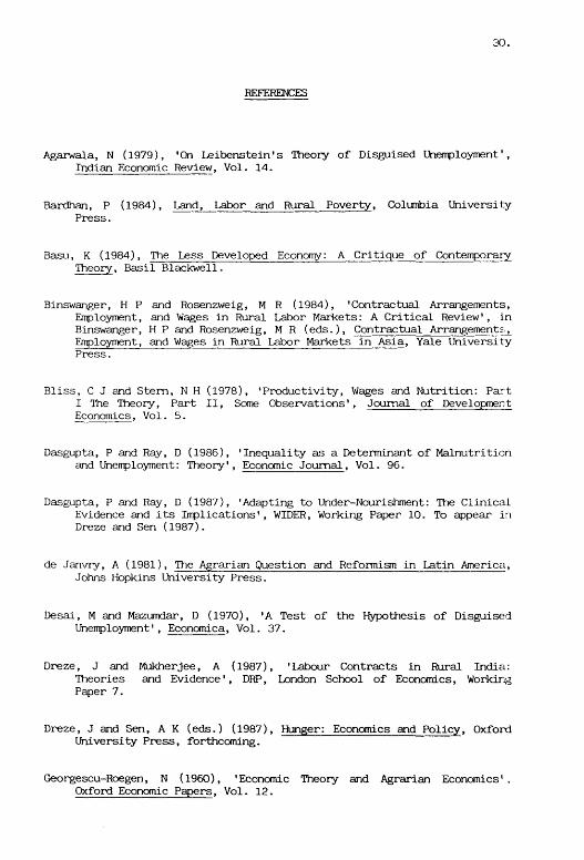
REFERENCES

Agarwala, N (1979), 'On Leibenstein's Theory of Disguised Unemployment', Indian Economic Review, Vol. 14.

Bardhan, P (1984), Land, Labor and Rural Poverty, Columbia University Press.

Basu, K (1984), The Less Developed Economy: A Critique of Contemporary Theory, Basil Blackwell.

Binswanger, H P and Rosenzweig, M R (1984), 'Contractual Arrangements, Employment, and Wages in Rural Labor Markets: A Critical Review' , in Binswanger, H P and Rosenzweig, M R (eds.), Contractual Arrangements, Employment, and Wages in Rural Labor Markets in Asia, Yale University Press.

Bliss, C J and Stem, N H (1978), 'Productivity, Wages and Nutrition: Part I The Theory, Part II, Some Observations', Journal of Development Economics, Vol. 5.

Dasgupta, P and Ray, D (1986), 'Inequality as a Determinant of Malnutrition and Unemployment: Theory', Economic Journal, Vol. 96.

Dasgupta, P and Ray, D (1987), 'Adapting to Under-Nourishment: The Clinical Evidence and its Implications' , WIDER, Working Paper 10. To appear in Dreze and Sen (1987).

de Janvry, A (1981), The Agrarian Question and Reformism in Latin America, Johns Hopkins University Press.

Desai, M and Mazumdar, D (1970), 'A Test of the Hypothesis of Disguised Unemployment', Economica, Vol. 37.

Dreze, J and Mukherjee, A (1987), 'Labour Contracts in Rural India: Theories and Evidence', DRP, London School of Economics, Working Paper 7.

Dreze, J and Sen, A K (eds.) (1987), Hunger: Economics and Policy, Oxford University Press, forthcoming.

Georgescu-Roegen, N (1960), 'Economic Theory and Agrarian Economies', Oxford Economic Papers, Vol. 12.

31.

Guha, A (1987), 'Consumption, Efficiency Wage and Surplus Labour', mimeo, J.N.U., New Delhi.

Islam, N (1965), 'Concept and Measurement of Unemployment and Underemployment in Developing Economies', International Labour Review, March.

Kao, C H C, Anschel, K R and Eicher, C (1964), 'Disguised Unemployment in Agriculture', in Eicher, C and Witt, L (eds.), Agriculture in Economic Development, McGraw-Hill.

Leibenstein, H (1957), 'The Theory of Underemployment in Backward Economies', Journal of Political Economy, Vol. 65.

Leibenstein, H (1958), 'Underemployment in Backward Economies: Some Additional Notes', Journal of Political Economy, Vol. 66.

Mathur, A (1965), 'The Anatomy of Disguised Unemployment', Oxford Economic Papers, Vol. 17.

Mazumdar, D (1959), "The Marginal Productivity Theory of Wages and Disguised Unemployment', Review of Economic Studies, Vol. 26.

Mellor, J W (1967), 'Towards a Theory of Agricultural Development', in Southworth, H M and Johnson, B F (eds.), Agricultural Development and Economic Growth, Cornell University Press.

Mirrlees, J A (1975), 'Pure Theory of Underdeveloped Economies', in Reynolds, L G (ed.), Agriculture in Development Theory, Yale University Press.

Myrdal, G (1968), Asian Drama, Pantheon.

Navarrete, A and Navarrete, I M (1951), 'La subocupacion en las economias poco desarrolladas', El Trimestre Economico. English translation in International Economic Papers, 1953, Vol. 3.

Osmani, S R (1987), 'Nutrition and the Economics of Food: Implications of Some Recent Controversy', in Dreze and Sen (1987).

Paglin, M (1965), '"Surplus" Agricultural Labor and Development', American Economic Review, Vol. 55.

32.

Robinson, J (1937), Essays in The Theory of Employment, Macmillan.

Robinson, W C (1969), 'Types of Disguised Rural Unemployment and Some Policy Implications', Oxford Economic Papers, Vol. 21.

Rodgers, G B (1975), 'Nutritionally Based Wage Determination in the Low-Income Labour Market', Oxford Economic Papers, Vol. 27.

Rudra, A (1982), Indian Agricultural Economics: Myths and Realities, Allied Publishers.

Salop, J and Salop, S (1976), 'Self-selection and Turnovers in the Labour Market', Quarterly Journal of Economics, Vol. 40.

Schultz, T W (1964), Transforming Traditional Agriculture, Yale University Press.

Sen, A K (1966), 'Peasants and Dualism with or without Surplus Labour', Journal of Political Economy, Vol. 74.

Sen, A K (1967), 'Surplus Labour in India: A Critique of Schultz's Statistical Test', Economic Journal, Vol. 77.

Squire, L (1981), Employment Policy in Developing Countries, Oxford University Press.

Stiglitz, J E (1974), 'Alternative Theories of Wage Determination and Unemployment in LDCs: The Labour Turnover Model', Quarterly Journal of Economics, Vol. 88.

Stiglitz, J E (1976), 'The Efficiency Wage Hypothesis, Surplus Labour and the Distribution of Labour in LDCs', Oxford Economic Papers, Vol. 28.

Wonnacott, P (1962), 'Disguised and Overt Unemployment in Underdeveloped Economies', Quarterly Journal of Economics, Vol. 26.