A Turing Machine simulator for academic uses … · Conversion from and to the JFlap Turing Machine format. 1. 4 Extensions Possible extensions are: I. Two-tape features. ! 2! II

The candidate confirms that the work submitted is their own and the appropriate credit has been given where reference has been made to the work of others. I understand that failure to attribute material which is obtained from another source may be considered as plagiarism. (Signature of student) _______________________________

A Turing Machine simulator for

academic uses Alexandros James Psarras

Computer Science 2009/2010

i

Summary

The objective of this project was to develop a graphical Turing Machine simulator for academic uses.

The simulator, TuringSlashPython, has deterministic and non-deterministic features, using one tape or

two tapes. The output of the simulation is shown both graphically and in a more low-level format. The

users have the ability to save their work and to resume from where they stopped. When loading a

Turing Machine, the simulator will show all errors made. An autocorrect function is available that

will correct all the errors made and that will complete any missing data.

There are many other Turing Machines simulators that can be found online; the most noticeable one is

JFlap. TuringSlashPython can convert Turing Machines from and to the JFlap format. What makes

my simulator different from any other simulator are the loading features that output any error made

and the high-level commands that come with TuringSlashPython. These commands can help build

more complex Turing Machines.

ii

Acknowledgements

I would like to thank my supervisor, Dr Haiko Müller for his guidance, support and feedback

throughout the project. His help was greatly appreciated.

I would like to thank my friends and family for their support and help during my project.

A special thank you to Victoria Mawer for proof reading my report and for trying to understand how a

Turing Machine works.

Also, a big thank you to all the people who give up their time to help out with the project evaluation.

Finally, I would like to thank my mother and father. Had it not been for them, I would not be where I

am today.

iii

Contents

1 Introduction 1

1. 1 Aim . . . . . . . . . . . . . . . . . . . . . . . . . . . . . . . . . . . . . . . . . . . . . . . . . . . . . . . . 1

1. 2 Objectives . . . . . . . . . . . . . . . . . . . . . . . . . . . . . . . . . . . . . . . . . . . . . . . . . . . 1

1. 3 Minimum Requirements . . . . . . . . . . . . . . . . . . . . . . . . . . . . . . . . . . . . . . . . 1

1. 4 Extensions . . . . . . . . . . . . . . . . . . . . . . . . . . . . . . . . . . . . . . . . . . . . . . . . . . . 1

1. 5 Deliverables . . . . . . . . . . . . . . . . . . . . . . . . . . . . . . . . . . . . . . . . . . . . . . . . . . 2

1. 6 Initial Project Schedule . . . . . . . . . . . . . . . . . . . . . . . . . . . . . . . . . . . . . . . . . 2

1. 7 Final Project Schedule . . . . . . . . . . . . . . . . . . . . . . . . . . . . . . . . . . . . . . . . . . 3

2 Background Reading and Research 4 2. 1 Overview . . . . . . . . . . . . . . . . . . . . . . . . . . . . . . . . . . . . . . . . . . . . . . . . . . . . 4

2. 2 Variations of Turing Machines . . . . . . . . . . . . . . . . . . . . . . . . . . . . . . . . . . . 4

2. 2. 1 Deterministic Turing Machines . . . . . . . . . . . . . . . . . . . . . . . . . . . 4

2. 2. 2 Non-deterministic Turing Machines . . . . . . . . . . . . . . . . . . . . . . . 6

2. 2. 3 Multi-tape Turing Machines . . . . . . . . . . . . . . . . . . . . . . . . . . . . . 7

2. 2. 4 Universal Turing Machines . . . . . . . . . . . . . . . . . . . . . . . . . . . . . . 7

2. 3 Turing Machine simulators . . . . . . . . . . . . . . . . . . . . . . . . . . . . . . . . . . . . . . 8

3 Project Management 9

3. 1 Introduction . . . . . . . . . . . . . . . . . . . . . . . . . . . . . . . . . . . . . . . . . . . . . . . . . . 9

3. 2 Personal Extreme Programming (PXP) . . . . . . . . . . . . . . . . . . . . . . . . . . . . . 9

3. 3 Evolutionary Prototyping . . . . . . . . . . . . . . . . . . . . . . . . . . . . . . . . . . . . . . . . 10

3. 3. 1 Version 1.0 . . . . . . . . . . . . . . . . . . . . . . . . . . . . . . . . . . . . . . . . . . . 11

3. 3. 2 Version 1.1 . . . . . . . . . . . . . . . . . . . . . . . . . . . . . . . . . . . . . . . . . . . 11

3. 3. 3 Version 1.2 . . . . . . . . . . . . . . . . . . . . . . . . . . . . . . . . . . . . . . . . . . . 11

3. 3. 4 Version 1.3 . . . . . . . . . . . . . . . . . . . . . . . . . . . . . . . . . . . . . . . . . . . 12

3. 3. 5 Version 1.4 . . . . . . . . . . . . . . . . . . . . . . . . . . . . . . . . . . . . . . . . . . . 12

3. 3. 6 Version 1.5 . . . . . . . . . . . . . . . . . . . . . . . . . . . . . . . . . . . . . . . . . . . 12

iv

3. 3. 7 Version 1.6 . . . . . . . . . . . . . . . . . . . . . . . . . . . . . . . . . . . . . . . . . . . 12

3. 4 Software Justification . . . . . . . . . . . . . . . . . . . . . . . . . . . . . . . . . . . . . . . . . . . 13

4 Implementation 15

4. 1 Iteration 1 . . . . . . . . . . . . . . . . . . . . . . . . . . . . . . . . . . . . . . . . . . . . . . . . . . . . 15

4. 2 Iteration 2 . . . . . . . . . . . . . . . . . . . . . . . . . . . . . . . . . . . . . . . . . . . . . . . . . . . . 18

4. 3 Iteration 3 . . . . . . . . . . . . . . . . . . . . . . . . . . . . . . . . . . . . . . . . . . . . . . . . . . . . 23

4. 4 Iteration 4 . . . . . . . . . . . . . . . . . . . . . . . . . . . . . . . . . . . . . . . . . . . . . . . . . . . . 27

4. 5 Iteration 5 . . . . . . . . . . . . . . . . . . . . . . . . . . . . . . . . . . . . . . . . . . . . . . . . . . . . 29

4. 6 Iteration 6 . . . . . . . . . . . . . . . . . . . . . . . . . . . . . . . . . . . . . . . . . . . . . . . . . . . . 31

4. 7 Iteration 7 . . . . . . . . . . . . . . . . . . . . . . . . . . . . . . . . . . . . . . . . . . . . . . . . . . . . 33

4. 8 Conclusion . . . . . . . . . . . . . . . . . . . . . . . . . . . . . . . . . . . . . . . . . . . . . . . . . . . 34

5 High-level commands 35

5. 1 Introduction . . . . . . . . . . . . . . . . . . . . . . . . . . . . . . . . . . . . . . . . . . . . . . . . . . 35

5. 2 High-level commands for one tape . . . . . . . . . . . . . . . . . . . . . . . . . . . . . . . . 35

5. 2. 1 The “go2start(q0, q1)” command . . . . . . . . . . . . . . . . . . . . . . . . . . 35

5. 2. 2 The “go2end(q0, q1)” command . . . . . . . . . . . . . . . . . . . . . . . . . . 36

5. 2. 3 The “add2start(q0, q1, 1)” command . . . . . . . . . . . . . . . . . . . . . . . 36

5. 2. 4 The “add2end(q0, q1, 1)” command . . . . . . . . . . . . . . . . . . . . . . . 36

5. 2. 5 The “find(q0, q1, q2, 1, D)” command . . . . . . . . . . . . . . . . . . . . . 37

5. 2. 6 The “replace(q0, q1, q2, 1, a, D)” command . . . . . . . . . . . . . . . . . 37

5. 2. 7 The “replaceall(q0, q1, q2, 1, a)” command . . . . . . . . . . . . . . . . . 37

5. 2. 8 The “remove(q0, q1, 1)” command . . . . . . . . . . . . . . . . . . . . . . . . 38

5. 2. 9 The “copy(q0, q1, #, %)” command . . . . . . . . . . . . . . . . . . . . . . . 38

5. 2. 10 The “compare(q0, q1, q2, #, %)” command . . . . . . . . . . . . . . . . 40

5. 3 High-level commands for two tapes . . . . . . . . . . . . . . . . . . . . . . . . . . . . . . . 42

5. 3. 1 The “go2start(q0, q1)” command . . . . . . . . . . . . . . . . . . . . . . . . . . 42

5. 3. 2 The “go2start1(q0, q1)” and “go2start2(q0, q1)” commands . . . . 42

5. 3. 3 The “go2end(q0, q1)” command . . . . . . . . . . . . . . . . . . . . . . . . . . 43

5. 3. 4 The “go2end1(q0, q1)” and “go2end2(q0, q1)” commands . . . . . . 43

5. 3. 5 The “add2start(q0, q1, 1)” command . . . . . . . . . . . . . . . . . . . . . . . 43

v

5. 3. 6 The “add2start1(q0, q1, 1)” and “add2start2(q0, q1, 1)”

commands . . . . . . . . . . . . . . . . . . . . . . . . . . . . . . . . . . . . . . . . . . . 44

5. 3. 7 The “add2end(q0, q1, 1)” command . . . . . . . . . . . . . . . . . . . . . . . 44

5. 3. 8 The “add2end1(q0, q1, 1)” and “add2end2(q0, q1, 1)”

commands . . . . . . . . . . . . . . . . . . . . . . . . . . . . . . . . . . . . . . . . . . . 44

5. 3. 9 The “find(q0, q1, q2, 1, 2, D)” command . . . . . . . . . . . . . . . . . . . 45

5. 3. 10 The “find1(q0, q1, q2, 1, D)” and “find2(q0, q1, q2, 1, D)”

commands . . . . . . . . . . . . . . . . . . . . . . . . . . . . . . . . . . . . . . . . . . . 45

5. 3. 11 The “replace(q0, q1, q2, 1, 2, 3, 4, D)” command . . . . . . . . . . . . 45

5. 3. 12 The “replace1(q0, q1, q2, 1, a, D)” and “replace2(q0, q1, q2, 1, a, D)”

commands . . . . . . . . . . . . . . . . . . . . . . . . . . . . . . . . . . . . . . . . . . . 46

5. 3. 13 The “replaceall(q0, q1, q2, 1, 2, 3, 4)” command . . . . . . . . . . . . . 46

5. 3. 14 The “replaceall1(q0, q1, q2, 1, a)” and “replaceall2(q0, q1, q2, 1, a)”

commands . . . . . . . . . . . . . . . . . . . . . . . . . . . . . . . . . . . . . . . . . . . 46

5. 3. 15 The “remove(q0, q1, 1, 2)” command . . . . . . . . . . . . . . . . . . . . . . 47

5. 3. 16 The “remove1(q0, q1, 1)” and “remove2(q0, q1, 1)”

commands . . . . . . . . . . . . . . . . . . . . . . . . . . . . . . . . . . . . . . . . . . . 47

5. 3. 17 The “copy(q0, q1, #, %)” command . . . . . . . . . . . . . . . . . . . . . . . 47

5. 3. 18 The “copy1(q0, q1, #, %)” and “copy2(q0, q1, #, %)”

commands . . . . . . . . . . . . . . . . . . . . . . . . . . . . . . . . . . . . . . . . . . . 48

5. 3. 19 The “compare(q0, q1, q2, #, %)” command . . . . . . . . . . . . . . . . . 48

5. 3. 20 The “compare1(q0, q1, q2, #, %)” and “compare2(q0, q1, q2, #, %)”

commands . . . . . . . . . . . . . . . . . . . . . . . . . . . . . . . . . . . . . . . . . . . 49

6 Evaluation 50 6. 1 Introduction . . . . . . . . . . . . . . . . . . . . . . . . . . . . . . . . . . . . . . . . . . . . . . . . . . 50

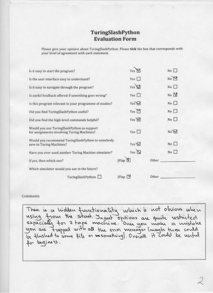
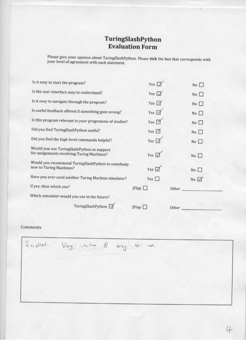
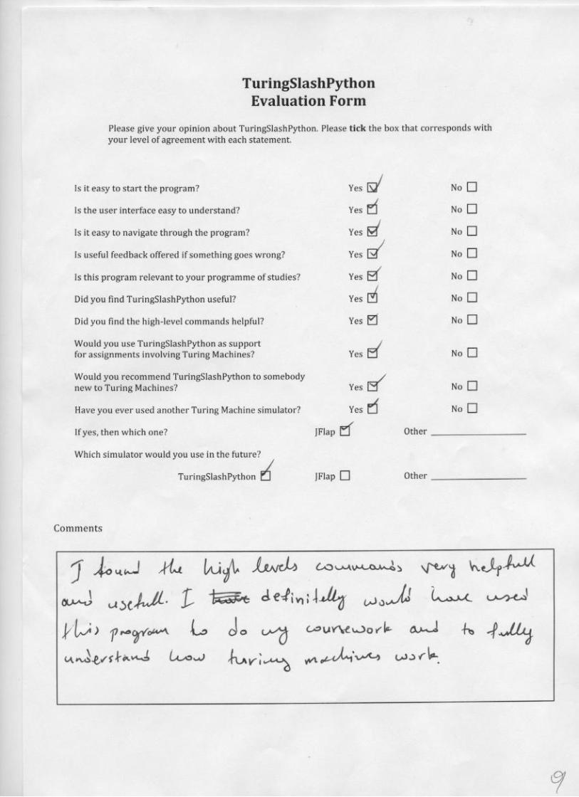
6. 2 User Feedback . . . . . . . . . . . . . . . . . . . . . . . . . . . . . . . . . . . . . . . . . . . . . . . . 50

6. 3 TuringSlashPython Evaluation . . . . . . . . . . . . . . . . . . . . . . . . . . . . . . . . . . . . 52

6. 4 Comparison with JFlap . . . . . . . . . . . . . . . . . . . . . . . . . . . . . . . . . . . . . . . . . . 55

References 56

A Personal Reflection 58

vi

B Schedules 60

C How-to tips 63

D TuringSlashPython in Action 70

E High-level command examples 97

F In the CD 145

G Tutorial and feedback forms 146

1

Chapter 1: Introduction

1. 1 Aim

The aim of the project is to produce a Turing Machine simulator for academic uses.

1. 2 Objectives

The main objective of the project is to produce a Turing Machine simulator in

Python. The steps to achieve the aim of the project are:

I. Analysis of the problem and investigation of other Turing Machine simulators.

II. Formulation of an appropriate development process.

III. Development of the graphical simulator in wxPython.

IV. Evaluation of the final version of the program.

1. 3 Minimum Requirements

The minimum requirements are:

I. The creation of a one-tape deterministic Turing Machine.

II. The use of XML to input and output Turing Machines.

III. Conversion from and to the JFlap Turing Machine format.

1. 4 Extensions

Possible extensions are:

I. Two-tape features.

2

II. Non-deterministic features.

III. A more detailed output, including the initial, final and maximum length of the tape.

IV. Autofill / autocorrect features.

V. High-level command features.

VI. Comparison of different Turing Machines.

VII. Combination of multiple Turing Machines in one simulation.

1. 5 Deliverables

With this report, I submit a CD containing the final version of my Python Turing

Machine simulator, TuringSlashPython.

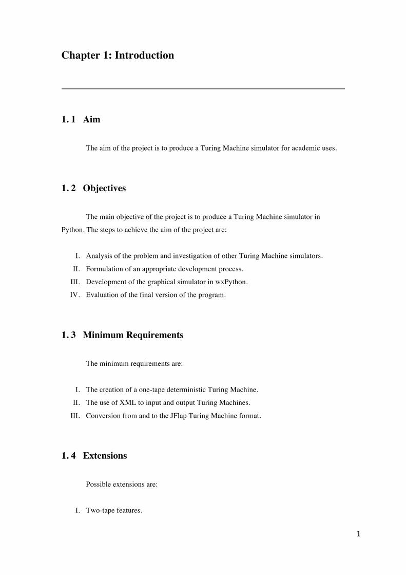
1. 6 Initial Project Schedule

Figure 1.1: Initial Project Schedule

3

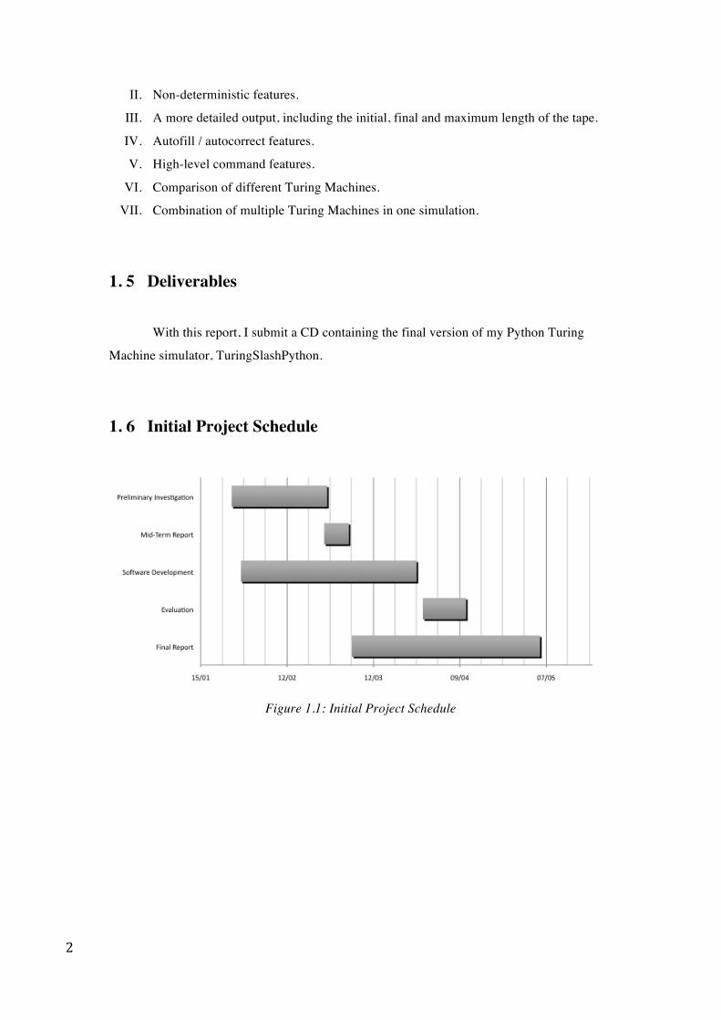
1. 7 Final Project Schedule

Figure 1.2: Final Project Schedule

Figure 1.2 shows the final schedule of the project including the breakdown of the

software development into seven iterations (see Paragraph 4.2 in Chapter 4). In Figure 1.1,

the evaluation the project was scheduled for the 28th of May. However since a major part of

the evaluation is derived from user feedback, this task was delayed by 22 days due to the

Easter break. This change is reflected in Figure 1.2. The final update on Figure 1.2 is the

addition of the ‘Proof reading and corrections’ task starting on the 5th of May and ending on

the 12th of May. Larger versions of Figures 1.1 and 1.2 can be found in Appendix B, including

the start and ending dates of each task.

4

Chapter 2: Background Reading and Research

2. 1 Overview

A Turing Machine (TM) is a theoretical computing machine, first described by Alan

Turing [1] that investigates the limits of computation. A Turing Machine has three parts:

1. An infinite tape that is divided into cells. This tape can move left and right.

2. A head that can read the cells on the tape and write symbols in the cells. The head has

a property known as “state”, that determines the action the head will take.

3. A set of instructions on how the head should move on the tape and how it should

change the symbol in each cell.

A move[2] of a Turing Machine is a function of the state on the head and the symbol

on the cell being scanned. In one move:

1. The state will change. However, the next state could be the same as the current state.

2. A tape symbol will be written on the cell being scanned according to the instructions.

If the symbol to be written and the current symbol are the same, then no change is

made.

3. The tape will move left or right.

The Turing Machine begins the computation when the input is given. The head goes

to the cell with the first symbol of the input. The Turing Machine moves until it reaches an

accepting state or a rejecting state, also known as final states. If no final states are reached,

then the computation never halts.

2. 2 Variations of Turing Machines

2. 2. 1 Deterministic Turing Machines

A deterministic Turing Machine (DTM) is described by the 7-tuple M = (Q, Σ, Γ, δ,

5

q0, b, F)[2], where:

• Q: is the finite set of states of the finite control.

• Σ: is the finite set of input symbols (alphabet).

• Γ: is the complete set of tape symbols (tape alphabet), Σ ⊆ Γ \ {b}.

• δ: is the transition function. The arguments of δ(q, X) are a state q and a tape

symbol X. If it’s defined, the value of δ(q, X) is the triple (p, Y, D), where:

1. p is the next state, in Q.

2. Y is the symbol, in Γ, replacing the symbol in the cell being

scanned.

3. D is the direction, either left (L) or right (R), telling us in which

direction the head will move.

δ: (Q \ F) x Γ Q x Γ x {L, R}

• q0: is the start state, q0 ∈ Q.

• b: is the blank symbol, b ∈ Γ and b ∉ Σ.

• F: is the set of final or halting states, F ⊂ Q.

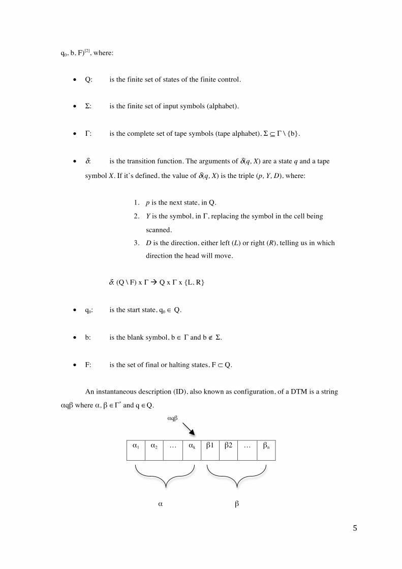
An instantaneous description (ID), also known as configuration, of a DTM is a string

αqβ where α, β ∈Γ* and q ∈Q.

αqβ

α1 α2 … αk β1 β2 … βn

α β

6

We do not distinguish between IDs that differ in prefix and/or suffix in {b}*. A move

of a Turing Machine M is described by ⊢M, or just ⊢ if M is understood. The symbol ⊢ *M, or

just ⊢ * if M is understood, represents zero or move moves of the Turing Machine so that:

αapbβ ⊢M αacqβ ⇔ δ (p, b) = (q, c, R)

αapbβ ⊢M αqacβ ⇔ δ (p, b) = (q, c, L)

where p, q ∈ Q, a, b, c ∈ Γ and α, β ∈Γ*

The language accepted by M is denoted by:

L(M) = { w ∈Σ*, | ∃α ∈ Γ* ∃β ∈ Γ* (q0w ⊢ *M αpβ) }, where p ∈ F

2. 2. 2 Non-deterministic Turing Machines

A non-deterministic Turing Machine (NTM) is a DTM that has more than one

available transition in at least one point. For every possible transition, a new ‘parallel’ run is

created using that transition. NTMs are defined just like deterministic Turing Machines,

however the transition function δ is different. The arguments of δ(q, X) are a state q and a tape

symbol X. If it’s defined, the value of δ(q, X) is a set of triples {(p1, Y1, D1), (p2, Y2, D2),…(pk,

Yk, Dk)}, where:


2. Y is the symbol, in Γ, replacing the symbol in the cell being scanned.

3. D is the direction, either left (L) or right (R), telling us in which direction the

head will move.

δ: (Q \ F) x Γ P(Q x Γ x {L, R}), where P denotes a power set

The instantaneous description of a NTM is defined as for a DTM but the successor ID is not

unique. NTMs are equivalent to DTMs and it is possible to simulate a NTM with a DTM.

7

2. 2. 3 Multi-tape Turing Machines

Multi-tape Turing Machines work in a similar manner to single-tape Turing Machines.

Each tape i has its own tape alphabet Γi and its own head. In many of the following chapters,

the tape alphabet Γ of a multi-tape Turing Machine is described as the product of the tape

alphabet of each tape. For example, the tape alphabet of a two-tape TM is Γ = Γ1 x Γ2, where

Γ1 is the tape alphabet of tape one and Γ2 is the tape alphabet of tape two. At each step, the

Turing Machine reads the symbols under each head and acts according to the instructions.

Each head reads and write symbols only on its tape. The direction each head moves could be

different. The Turing Machine loops and halts just like any other single-tape Turing Machine.

For a two-tape TM the arguments of the transition function δ(q, A, B) are a state q, a tape

symbol A on tape one and a tape symbol B on tape two. If it’s defined, the value of δ(q, A, B)

is the quintuple (p, X, Y, D1, D2) where:


2. X is the symbol in Γ1, replacing the symbol in the cell being scanned on tape

one.

3. Y is the symbol in Γ2, replacing the symbol in the cell being scanned on tape

two.

4. D1 is the direction, either left (L) or right (R), telling us in which direction the

head on tape one will move.

5. D2 is the direction, either left (L) or right (R), telling us in which direction the

head on tape two will move.

2. 2. 4 Universal Turing Machines

A Universal Turing Machine[3] can simulate itself. A Universal Turing Machine U

takes as its input the description of an arbitrary Turing Machine M with the input w of the

tape of M, this string is denoted by <M, w>. The Universal Turing Machine U simulates the

Turing Machine on the input w. If M reaches a final state on the given input w, then U will

reach the same final state if <M, w> is the input.

8

2. 3 Turing Machine simulators

Many Turing Machine simulators can be found on the Internet but the most used

simulator is JFlap[4,5]. Amongst other features, JFlap simulates deterministic and non-

deterministic Turing Machines using up to 5 tapes. It can also simulate Universal Turing

Machines. It also gives the user various options when inputting the tape:

• Step

Going through each move of the TM, step by step.

• Fast Run

Computing the TM in background and outputting the final solution.

• Multiple Runs

Inputting multiple tapes and running them one at a time.

JFlap has some autofill features. If a value of δ(q, X) is missing then it is assumed

that the value missing is the triple (r, Y, D), where r is the rejecting state. JFlap can also

combine Turing Machine. However on the downside, JFlap does not load the Turing

Machine, so the errors in the machine are not outputted. When the user runs a simulation,

JFlap does not do any checks to determine the correctness of the input as it is assumed to be

correct. Also, JFlap has no high-level command features; all the commands given are low-

level commands in the form δ(q, X) = (r, Y, D). See Section 6.4 of Chapter 6 for a side-by-

side comparison of JFlap and TuringSlashPython.

9

Chapter 3: Project Management

3. 1 Introduction

“A methodology is a set of guidelines or principles that can be tailored and applied to

a specific situation. In a project environment, these guidelines might be a list of things to do.

A methodology could also be a specific approach, template, forms, and even checklists used

over the project”[6]. There are many types of methodologies currently used. Each

methodology has its advantages and disadvantages. There is no methodology that suits all

projects so when managing a project, it is important to select a reliable and well-suited

methodology.

The majority of methodologies are designed for large projects so the selected

methodology would have to be modified to suit a small project for single person. After careful

consideration of all the possible methodologies, I decided to use the Personal Extreme

Programming (PXP) methodology (see Section 3.2) with Evolutionary Prototyping techniques

(see Section 3.3).

3. 2 Personal Extreme Programming (PXP)

The Personal Extreme Programming (PXP)[7] methodology is a combination of

Extreme Programming (XP) and Personal Software Process (PSP). XP is one of the best

known and widely used agile methods[8]. All the coding is done in pairs. Many releases are

published very fast until the client is happy with the final version. XP is more suitable for

small projects as it is too minimal for larger projects. PSP was designed to improve the

quality and productivity of software engineers who are working on an individual project[9].

The aim of the PSP is to enhance the standards of a one-man project and to produce results on

schedule, with little or no errors.

My selected methodology is PXP as it is suitable for one programmer instead of two.

PXP inherits XP and PSP emphasis on providing quality products through vigorous testing.

PXP was modified to suit this project, keeping only the features that are relevant.

10

The first step in managing this project is to produce the minimum requirements and to

create User Stories from the requirements. Each User Story is then translated into a feature of

the program. Each feature of the program was discussed in the weekly meeting with my

project supervisor before it was implemented. Feedback was provided on the characteristics

of each feature. The implementation of each feature would begin once its attributes were

established. Once a new feature has been created, the feature will undergo a number of tests

that examine if it meets its requirements. If a mistake has been found then the feature will be

re-implemented so that its attributes are as expected.

The first minimum requirement, “The creation of a one-tape deterministic Turing

Machine”, was implemented in the second version of the program (see Section 3.3.2). The

second and third minimum requirements, “The use of XML to input and output Turing

Machines” and “Conversion from and to the JFlap Turing Machine format”, were both

implemented in the third version of the program (see Section 3.3.3).

The minimum requirements needed twelve days to be implemented. So at this stage

of the project, it was agreed in the weekly meeting to explore the possible extensions of the

project. The first two extensions incorporate two-tape features and non-deterministic features

to the program (see Section 3.3.4 and Section 3.3.5). Both extensions took eleven days to be

included in the program. The implementation of these features took longer that expected. The

next extension, introducing autofill and autocorrect features (see Section 3.3.6), also took

longer that expected. This is because this version of the program should correct the input of

four different types of Turing Machines – one-tape DTM, one-tape NTM, two-tape DTM and

two-tape NTM. This task turned out to be more complex that originally estimated. The forth

and last extension introduces high-level commands (see Section 3.3.7). 10 one-tape and 29

two-tape high-level commands were implemented. These commands were selected in the

weekly meetings and their behaviour was discussed and analyzed before they were

implemented.

At this point, I decided to stop implementing extensions of the program as I already

dedicated 78 days to software development and it was time to start the evaluation of the

project and the write-up.

3. 3 Evolutionary Prototyping

Evolutionary Prototyping[8] is one of variation of Software Prototyping. A prototype

is a partially finished version of the software program being created. The objective of

Evolutionary Prototyping is to rapidly produce the working system, this is done though a

11

prototype that is continuously remodeled and improved. The system is developed and

delivered in series of increments. In my case, seven different versions of the Turing Machine

simulator were implemented before the final system was completed. In every new version of

the system, major new features are included. This ensures that if something goes wrong with

the coding, I have a previous version from which I can restart the implementation of the new

feature.

3. 3. 1 Version 1. 0

1st Iteration – Start Date: 28/01/10, End Date: 01/02/10, Duration: 4 days

This is the initial version. The system is a simple Graphical User Interface (GUI)

converted from pen and paper models of the final version. The prototype has no Turing

Machine simulator features. In later versions, more elements are included in the GUI that

supports the new features (see Section 4.1).

3. 3. 2 Version 1. 1

2nd Iteration – Start Date: 01/02/10, End Date: 05/02/10, Duration: 4 days

In this version, one-tape simulator features are integrated to the GUI. The user can

enter the Turing Machine details. When the input is executed, the simulator will check the

validity of the input and outputs any errors. If the input is correct, then the simulator will run

successfully (see Section 4.2).

3. 3. 3 Version 1. 2

3rd Iteration – Start Date: 05/02/10, End Date: 09/02/10, Duration: 4 days

In version 1.2, the user can open and save Turing Machines. This is done with the use

of Extensible Markup Language (XML). The user is also able to convert from and to the

JFlap format (see Section 4.3).

12

3. 3. 4 Version 1. 3

4th Iteration – Start Date: 09/02/10, End Date: 12/02/10, Duration: 3 days

Two-tape simulator features are integrated to the GUI in version 1.3. The user is able

to change the number of tapes in the interface (see Section 4.4).

3. 3. 5 Version 1. 4


In version 1.4, the user can run one tape and two tape non-deterministic Turing

Machines (see Section 4.5).

3. 3. 6 Version 1. 5


This version introduces autofill and autocomplete features. If any errors are found

then they will be corrected (see Section 4.6).

3. 3. 7 Version 1. 6


This is the final version of the Turing Machine simulator. 10 one-tape and 29 two-

tape high-level commands are introduced (see Section 4.7).

13

3. 4 Software Justification

The first major decision I had to make was whether I should extend an existing

Turing Machine simulator or build one from scratch. There are many Turing Machine

simulators that can be found online[4, 10-15]. The majority of simulators are written in Java and

can be modified to extend their features. However the only simulator I considered modifying

was JFlap as it is the only one that stands out. As mentioned earlier, amongst other features,

JFlap is used as a Turing Machine simulator. It was created in 1990 and since then it has

undergone a series of modifications by students of the Rensselaer Polytechnic Institute and

the Duke University.

The idea of altering and extending code that was not written by myself was not

appealing. Even if the code was well documented and comments were provided on how the

program works, valuable time would be lost to familiarise myself with the structure of the

code. On the other hand, by building a program from scratch I am in control of the design and

the properties of the program. It might be time consuming to create a new simulator from

scratch but in the long run it would be faster to extend my own code than code written by

many different people with different coding styles. The decision to build a Turing Machine

simulator from scratch influenced the choice of programming language.

Due to time constraints, I considered only three different programming languages for

this project. From experience with different programming languages, it is my opinion that the

use of an object-orientated programming language would be best suited for this project.

Whilst deciding which programming language to choose I had to consider the suitability to

the project and to my skills. The programming language would determine how long the

coding part of the project would take. Choosing a strong language that I am unfamiliar with

was out of the question. Therefore the three possible programming languages I could have

chosen were: Visual Basic (VB), Java and Python.

The first language I considered was VB. VB is an event-driven language that

provides a number of tools for developing applications with a GUI interface[16]. Programming

in VB would make it easy for me to complete the requirements of the project in half the time.

But VB was quickly dropped because:

1. VB is not cross-platform.

2. The use of VB is encouraged in the Rapid Application Development (RAD)

methodology[8] but not in the Personal Extreme Programming methodology.

14

3. It is my opinion that creating a TM simulator in VB is not suitable for a final

year project, as I do not find it challenging to write code in VB compared to

Java and Python.

By eliminating VB, the remaining languages were Java and Python. The next step

was to do a side-to-side comparison of both programming language so I could choose the best

suited for this project. Java and Python are both popular object-oriented languages that can

run on almost any computer. On one hand, Java is a very popular language, that is used

almost everywhere. Java combines the abilities of an interpreted language and a compiled

language. On the other hand, Python is easier and quicker to write and the code written is

cleaner. Python compiles whilst running the program, i.e. it interpreted, while Java is

compiled. This gives Python the upper hand as compiling, run and debugging the Java code

can be time consuming. Java is statically typed while Python is dynamically typed. My

opinion is that dynamically typed languages are stronger compared to statically typed

languages. Dynamically typed languages are more simple and flexible and improve

productivity as less time is spent writing code to initialize variables.

Both Python and Java have interface toolkits that would be used in the project. Java

has the Swing toolkit while Python has Tkinter and wxPython. Tkinter comes with the Python

distribution but it also comes with a steep learning curve. Also the widgets used are not native

to the operating system. wxPython does not come with the Python distribution and needs to

be downloaded and installed. In my opinion, this seems to be the only downside of wxPython

as the learning curve is steady and the wxPython widgets are native to any operating system

(OS). So the decision to choose wxPython over Tkinter was simple and easy. The comparison

of Swing and wxPython is similar to Java and Python. wxPython is less complicated, easier to

use and is not as lengthy as Swing. However Swing is faster and more stable that wxPython.

I decided to choose Python over Java because I have more experience writing code in

Python and wxPython. This and the simplicity of Python code made a great impact in my

decision. Not only I would be able to produce code faster in Python compared to Java, but

also anyone who would want to extend new features, would find it easier reading Python code

than Java code. Another reason why I chose Python is that debugging code would only take a

few minutes instead of hours or days in Java. This said, if the final year project had to be

developed over two semesters instead of one, then I would have chosen to implement the

Turing Machine simulator in Python and then I would convert the code to Java.

15

Chapter 4: Implementation

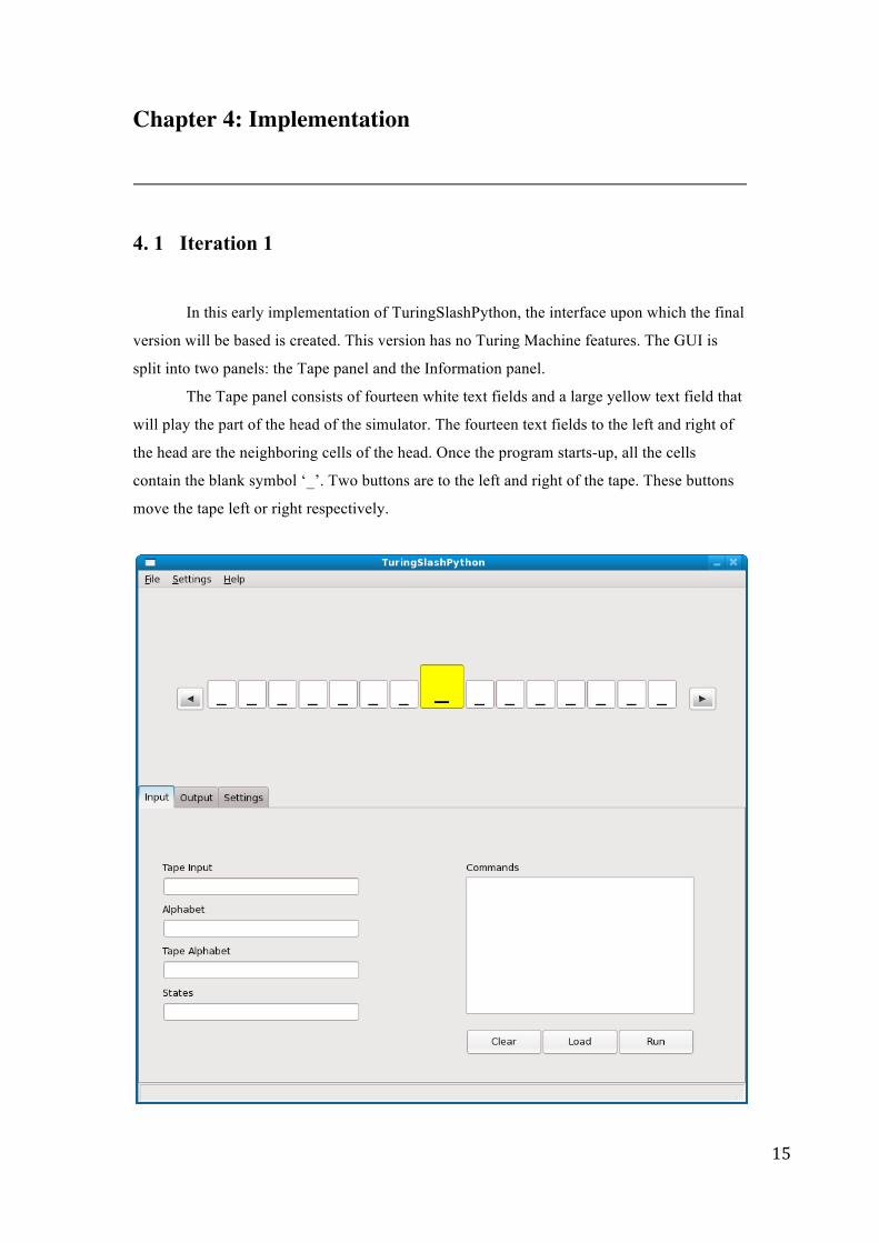
4. 1 Iteration 1

In this early implementation of TuringSlashPython, the interface upon which the final

version will be based is created. This version has no Turing Machine features. The GUI is

split into two panels: the Tape panel and the Information panel.

The Tape panel consists of fourteen white text fields and a large yellow text field that

will play the part of the head of the simulator. The fourteen text fields to the left and right of

the head are the neighboring cells of the head. Once the program starts-up, all the cells

contain the blank symbol ‘_’. Two buttons are to the left and right of the tape. These buttons

move the tape left or right respectively.

16

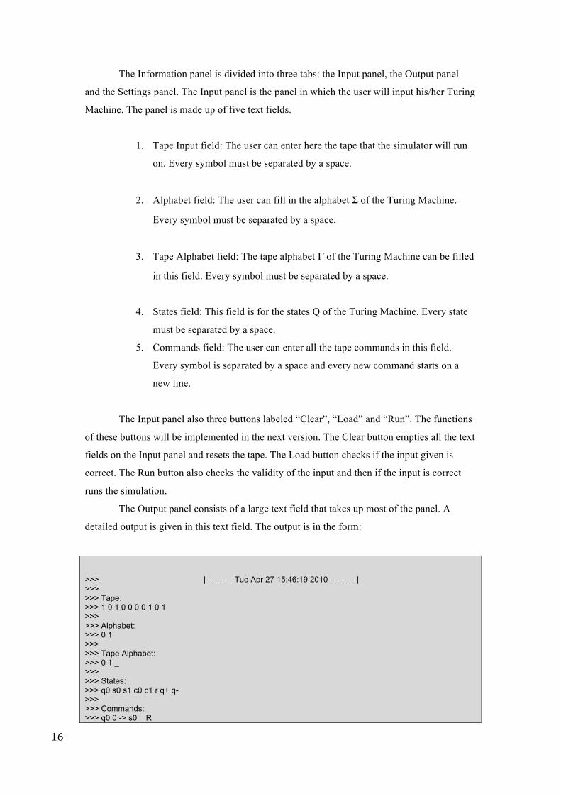
The Information panel is divided into three tabs: the Input panel, the Output panel

and the Settings panel. The Input panel is the panel in which the user will input his/her Turing

Machine. The panel is made up of five text fields.

1. Tape Input field: The user can enter here the tape that the simulator will run

on. Every symbol must be separated by a space.

2. Alphabet field: The user can fill in the alphabet Σ of the Turing Machine.

Every symbol must be separated by a space.

3. Tape Alphabet field: The tape alphabet Γ of the Turing Machine can be filled

in this field. Every symbol must be separated by a space.

4. States field: This field is for the states Q of the Turing Machine. Every state

must be separated by a space.

5. Commands field: The user can enter all the tape commands in this field.

Every symbol is separated by a space and every new command starts on a

new line.

The Input panel also three buttons labeled “Clear”, “Load” and “Run”. The functions

of these buttons will be implemented in the next version. The Clear button empties all the text

fields on the Input panel and resets the tape. The Load button checks if the input given is

correct. The Run button also checks the validity of the input and then if the input is correct

runs the simulation.

The Output panel consists of a large text field that takes up most of the panel. A

detailed output is given in this text field. The output is in the form:

>>> |---------- Tue Apr 27 15:46:19 2010 ----------| >>> >>> Tape: >>> 1 0 1 0 0 0 0 1 0 1 >>> >>> Alphabet: >>> 0 1 >>> >>> Tape Alphabet: >>> 0 1 _ >>> >>> States: >>> q0 s0 s1 c0 c1 r q+ q- >>> >>> Commands: >>> q0 0 -> s0 _ R

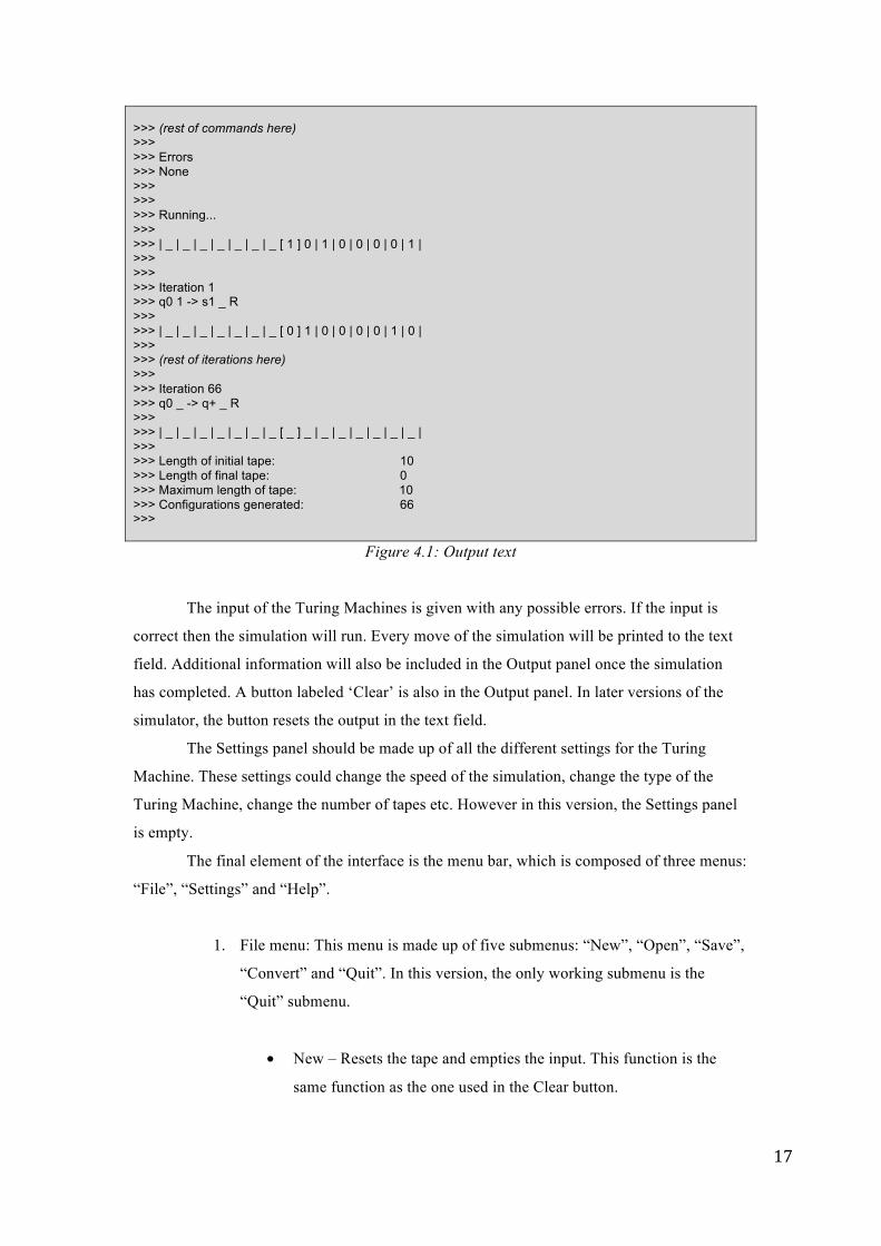
17

>>> (rest of commands here) >>> >>> Errors >>> None >>> >>> >>> Running... >>> >>> | _ | _ | _ | _ | _ | _ | _ [ 1 ] 0 | 1 | 0 | 0 | 0 | 0 | 1 | >>> >>> >>> Iteration 1 >>> q0 1 -> s1 _ R >>> >>> | _ | _ | _ | _ | _ | _ | _ [ 0 ] 1 | 0 | 0 | 0 | 0 | 1 | 0 | >>> >>> (rest of iterations here) >>> >>> Iteration 66 >>> q0 _ -> q+ _ R >>> >>> | _ | _ | _ | _ | _ | _ | _ [ _ ] _ | _ | _ | _ | _ | _ | _ | >>> >>> Length of initial tape: 10 >>> Length of final tape: 0 >>> Maximum length of tape: 10 >>> Configurations generated: 66 >>>

Figure 4.1: Output text

The input of the Turing Machines is given with any possible errors. If the input is

correct then the simulation will run. Every move of the simulation will be printed to the text

field. Additional information will also be included in the Output panel once the simulation

has completed. A button labeled ‘Clear’ is also in the Output panel. In later versions of the

simulator, the button resets the output in the text field.

The Settings panel should be made up of all the different settings for the Turing

Machine. These settings could change the speed of the simulation, change the type of the

Turing Machine, change the number of tapes etc. However in this version, the Settings panel

is empty.

The final element of the interface is the menu bar, which is composed of three menus:

“File”, “Settings” and “Help”.

1. File menu: This menu is made up of five submenus: “New”, “Open”, “Save”,

“Convert” and “Quit”. In this version, the only working submenu is the

“Quit” submenu.

• New – Resets the tape and empties the input. This function is the

same function as the one used in the Clear button.

18

• Open – Opens a dialog from which you can choose a XML file that

contains a Turing Machine. Clears the current input and replaces it

with the content of the file chosen. Useful if the user wants to review

a previously saved Turing Machine.

• Save – Opens a dialog from which you can create a new XML file or

replace an old file within which the input of the Turing Machine is

saved.

• Convert – This submenu gives you the option to convert from or to

the JFlap format.

• Quit – Exits the program.

2. Settings menu: This menu has all the elements found in the Settings tab of the

Information panel. In this version, the settings menu is empty.

3. Help menu: This menu is made up of two submenus: “How to” and “About”.

• How to: Displays tips on how to use TuringSlashPython. These tips

can be found in Appendix C.

• About: Displays a dialog that shows some information about the

program.

4. 2 Iteration 2

In this version, one-tape Turing Machine features are appended to the GUI. A new

text field is added to the Tape panel under the tape. This text field will output the current

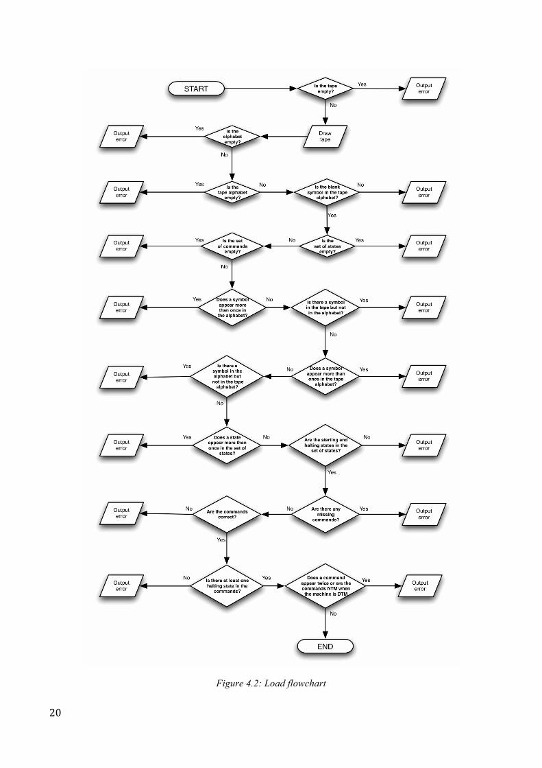
command used when the simulation is running. When the Load button is pressed, the validity

of the input will be checked (see Figure 4.2). Any mistake made will be outputted in the form

of a message dialog. The simulator will check if the tape is empty. If a value is given then it

will draw the tape to the interface. Then it will check if the other text fields are empty. If all

the text fields have a value then the simulator will examine the values given to determine the

correctness of the values. This is done through a series of questions (see Figure 4.2):

19

1. Is the tape empty?

2. Is the alphabet empty?

3. Is the tape alphabet empty?

4. Is the blank symbol in the tape alphabet?

5. Is the set of states empty?

6. Is the set of commands empty?

7. Does a symbol appear more than once in the alphabet?

8. Is there a symbol in the tape that is not in the alphabet?

9. Does a symbol appear more than once in the tape alphabet?

10. Is there a symbol in the alphabet that is not in the tape alphabet?

11. Does a state appear more than once in the set of states?

12. Are the starting and halting states in the set of states?

13. Are there any missing commands and in the right format?

14. Are the commands correct?

15. Is there at least one halting state in the commands?

16. Does a command appear twice?

17. Are the commands non-deterministic when the machine is deterministic?

20

Figure 4.2: Load flowchart

21

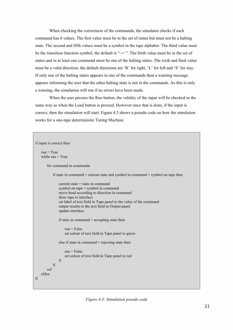
When checking the correctness of the commands, the simulator checks if each

command has 6 values. The first value must be in the set of states but must not be a halting

state. The second and fifth values must be a symbol in the tape alphabet. The third value must

be the transition function symbol, the default is “ -> ”. The forth value must be in the set of

states and in at least one command must be one of the halting states. The sixth and final value

must be a valid direction; the default directions are ‘R’ for right, ‘L’ for left and ‘S’ for stay.

If only one of the halting states appears in one of the commands then a warning message

appears informing the user that the other halting state is not in the commands. As this is only

a warning, the simulation will run if no errors have been made.

When the user presses the Run button, the validity of the input will be checked in the

same way as when the Load button is pressed. However once that is done, if the input is

correct, then the simulation will start. Figure 4.3 shows a pseudo code on how the simulation

works for a one-tape deterministic Turing Machine.

if input is correct then run = True while run = True for command in commands if state in command = current state and symbol in command = symbol on tape then current state = state in command symbol on tape = symbol in command move head according to direction in command draw tape to interface set label of text field in Tape panel to the value of the command output results to the text field in Output panel update interface if state in command = accepting state then run = False set colour of text field in Tape panel to green else if state in command = rejecting state then run = False set colour of text field in Tape panel to red fi fi rof elihw fi

Figure 4.3: Simulation pseudo code

22

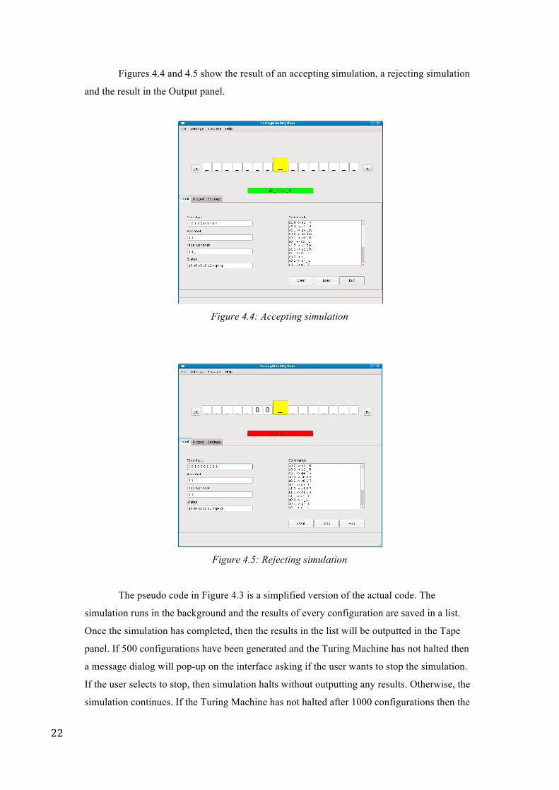
Figures 4.4 and 4.5 show the result of an accepting simulation, a rejecting simulation

and the result in the Output panel.

Figure 4.4: Accepting simulation

Figure 4.5: Rejecting simulation

The pseudo code in Figure 4.3 is a simplified version of the actual code. The

simulation runs in the background and the results of every configuration are saved in a list.

Once the simulation has completed, then the results in the list will be outputted in the Tape

panel. If 500 configurations have been generated and the Turing Machine has not halted then

a message dialog will pop-up on the interface asking if the user wants to stop the simulation.

If the user selects to stop, then simulation halts without outputting any results. Otherwise, the

simulation continues. If the Turing Machine has not halted after 1000 configurations then the

23

user is given the same option again. Every time the user decides to continue the next number

of configurations in which the pop-up dialog will appear will double, i.e. 500, 1000, 2000,

4000 and so on.

4. 3 Iteration 3

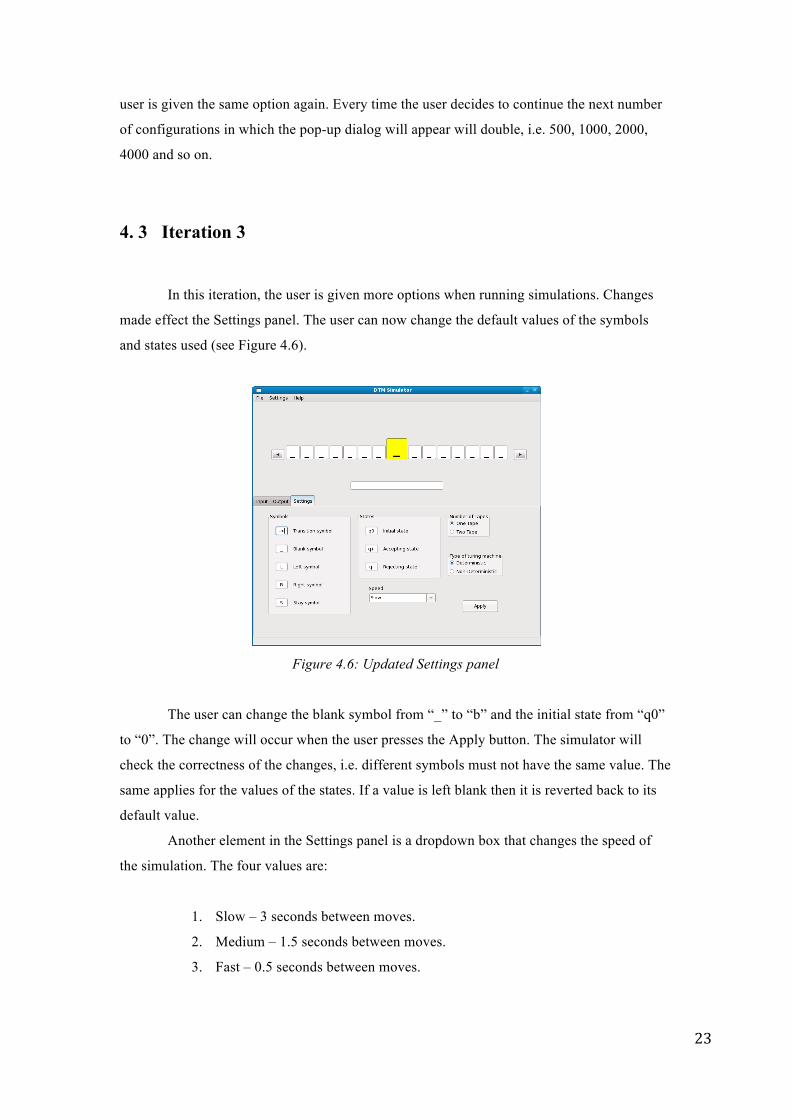
In this iteration, the user is given more options when running simulations. Changes

made effect the Settings panel. The user can now change the default values of the symbols

and states used (see Figure 4.6).

Figure 4.6: Updated Settings panel

The user can change the blank symbol from “_” to “b” and the initial state from “q0”

to “0”. The change will occur when the user presses the Apply button. The simulator will

check the correctness of the changes, i.e. different symbols must not have the same value. The

same applies for the values of the states. If a value is left blank then it is reverted back to its

default value.

Another element in the Settings panel is a dropdown box that changes the speed of

the simulation. The four values are:

1. Slow – 3 seconds between moves.

2. Medium – 1.5 seconds between moves.

3. Fast – 0.5 seconds between moves.

24

4. Compute – Only the final result in the list of configurations is outputted in

the Tape panel.

Two more elements are included in the Settings panel, two radio button fields. In later

versions, these radio buttons allow the user to change the type of the Turing Machine between

DTM and NTM and to change the number of tapes between one tape and two tapes.

Four more features are introduced in this iteration of the code:

1. Open (File -> Open)

2. Save (File -> Save)

3. Convert from JFlap (File -> Convert -> JFlap -> From JFlap)

4. Convert to JFlap (File -> Convert -> JFlap -> To JFlap)

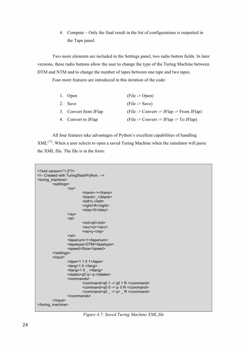
All four features take advantages of Python’s excellent capabilities of handling

XML[17]. When a user selects to open a saved Turing Machine when the simulator will parse

the XML file. The file is in the form:

<?xml version="1.0"?>  <turing_machine> <settings> <sy> <trans>-></trans> <blank>_</blank> <left>L</left> <right>R</right> <stay>S</stay> </sy> <st> <init>q0</init> <acc>q+</acc> <rej>q-</rej> </st> <tapenum>1</tapenum> <tapetype>DTM</tapetype> <speed>Slow</speed> </settings> <input> <tape>1 1 0 1</tape> <lang>1 0 </lang> <tlang>1 0 _ </tlang> <states>q0 q+ q-</states> <commands> <command>q0 1 -> q0 1 R </command> <command>q0 0 -> q- 0 R </command> <command>q0 _ -> q+ _ R </command> </commands> </input> </turing_machine>

Figure 4.7: Saved Turing Machine XML file

25

When saving a Turing Machine, all the input values are gathered and saved in a XML

file. Apart from saving the obvious information like the commands or the set of states, the

settings of the Turing Machine are also saved. When opening a saved Turing Machine file,

the input fields are filled with the values found in the file.

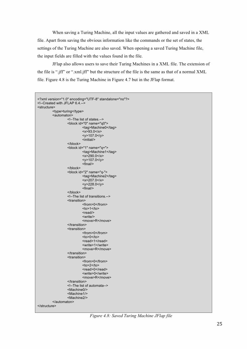
JFlap also allows users to save their Turing Machines in a XML file. The extension of

the file is “.jff” or “.xml.jff” but the structure of the file is the same as that of a normal XML

file. Figure 4.8 is the Turing Machine in Figure 4.7 but in the JFlap format.

<?xml version="1.0" encoding="UTF-8" standalone="no"?>  <structure> <type>turing</type> <automaton>  <block id="0" name="q0"> <tag>Machine0</tag> <x>93.0</x> <y>107.0</y> <initial/> </block> <block id="1" name="q+"> <tag>Machine1</tag> <x>290.0</x> <y>107.0</y> <final/> </block> <block id="2" name="q-"> <tag>Machine2</tag> <x>207.0</x> <y>228.0</y> <final/> </block>  <transition> <from>0</from> <to>1</to> <read/> <write/> <move>R</move> </transition> <transition> <from>0</from> <to>0</to> <read>1</read> <write>1</write> <move>R</move> </transition> <transition> <from>0</from> <to>2</to> <read>0</read> <write>0</write> <move>R</move> </transition>  <Machine0/> <Machine1/> <Machine2/> </automaton> </structure>

Figure 4.8: Saved Turing Machine JFlap file

26

Converting from the JFlap format is similar to opening Turing Machine that is in the

TuringSlashPython format (see Figures 4.7 and 4.8). The conversion will happen in the

background and the input fields are filled with the values converted from the file. The

conversion has successfully completed and the user can run the simulation or the save the

Turing Machine in the TuringSlashPython format (File -> Save). As you can see in Figure

4.8, the tags used in the JFlap format are different but the file can be easily converted.

The information for each state is between the “<block>” or “<state>” tags.

• The default name of the state is determined by the value of the attribute “id”.

E.g. 0 is the id of state q0, 1 is the id of the state q1.

• The user can change the name of the state. The new name is the value of the

attribute “name”.

• The values between the “<x>” and the “<y>” indicate the position of the state

on the screen.

• The tag “<initial/>” indicates that the state is the initial state.

• The tag “<final/>” indicates that the state is a halting state.

The information for every transition or command is between the “<transition>” tags.

• The value between the “<from>” tags indicates the current state.

• The value between the “<to>” tags indicates the new state.

• Between the “<read>” tags is the symbol on the tape that the head scans.

• If there is a single “</read>” tag then the head scans a blank symbol.

• Between the “<write>” tags is the new symbol that the head will write on the

tape.

• If there is a single “</write>” tag then the head writes a blank symbol to the

tape.

• The value between the “<move>” tags is the direction in which the head will

move, 'L', 'R' or 'S' (left, right or stay)

E.g.

<from>0</from>

<to>5</to>

<read></read>

<write></write>

<move>L</move>

27

In the TuringSlashPython translates to:

<command>q0 _ -> q5 _ L</command>

Figure 4.9: JFlap conversion menu

The user can also convert from the TuringSlashPython format to the JFlap format.

This function is similar to the save function (File -> Save). All the input values that are

relevant to JFlap are collected. The settings that apply only for TuringSlashPython, for

example the speed of simulation, are ignored. The information gathered is saved in the JFlap

file structure (see Figure 4.8).

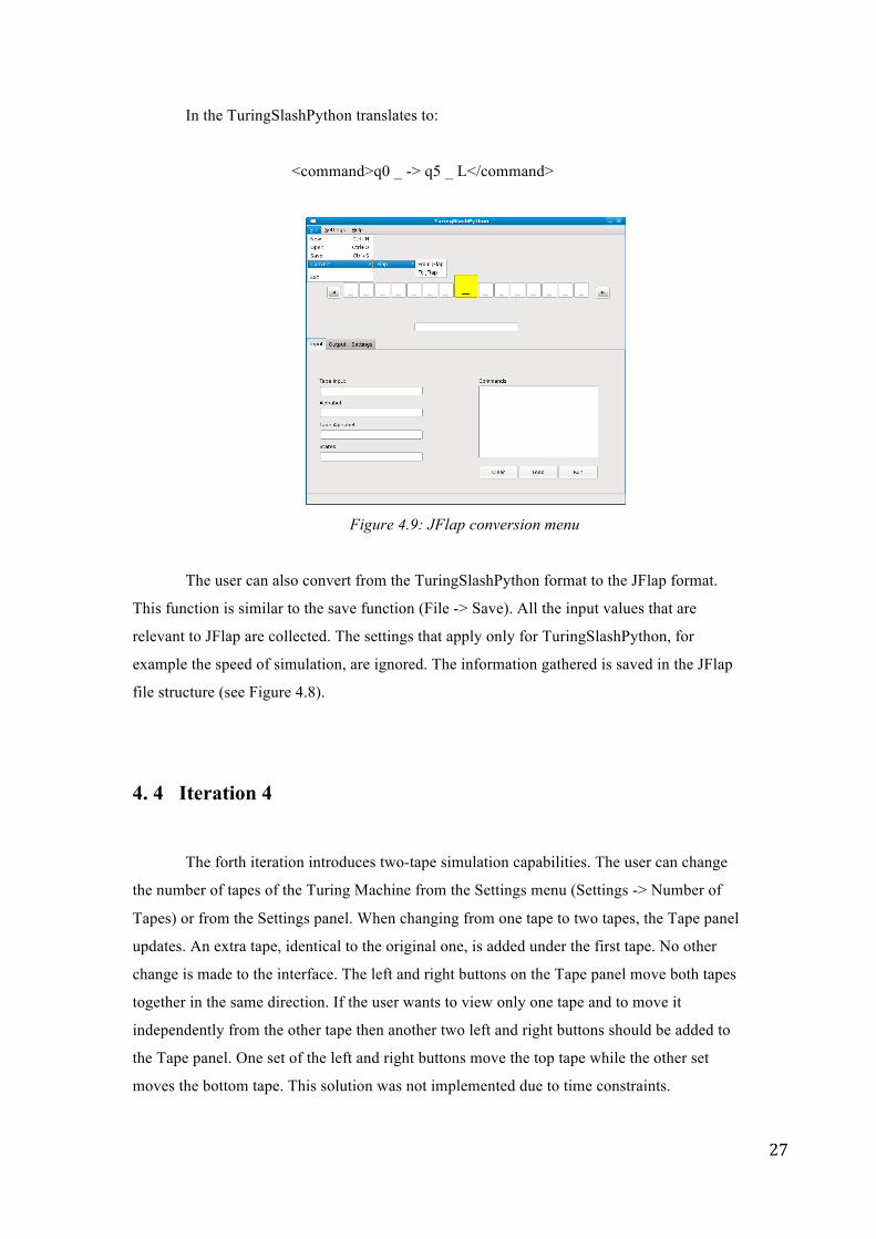
4. 4 Iteration 4

The forth iteration introduces two-tape simulation capabilities. The user can change

the number of tapes of the Turing Machine from the Settings menu (Settings -> Number of

Tapes) or from the Settings panel. When changing from one tape to two tapes, the Tape panel

updates. An extra tape, identical to the original one, is added under the first tape. No other

change is made to the interface. The left and right buttons on the Tape panel move both tapes

together in the same direction. If the user wants to view only one tape and to move it

independently from the other tape then another two left and right buttons should be added to

the Tape panel. One set of the left and right buttons move the top tape while the other set

moves the bottom tape. This solution was not implemented due to time constraints.

28

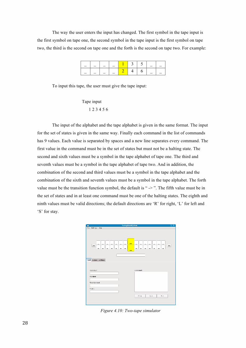
The way the user enters the input has changed. The first symbol in the tape input is

the first symbol on tape one, the second symbol in the tape input is the first symbol on tape

two, the third is the second on tape one and the forth is the second on tape two. For example:

_ _ _ _ 1 3 5 _ _ _ _ _ _ 2 4 6 _ _

To input this tape, the user must give the tape input:

Tape input

1 2 3 4 5 6

The input of the alphabet and the tape alphabet is given in the same format. The input

for the set of states is given in the same way. Finally each command in the list of commands

has 9 values. Each value is separated by spaces and a new line separates every command. The

first value in the command must be in the set of states but must not be a halting state. The

second and sixth values must be a symbol in the tape alphabet of tape one. The third and

seventh values must be a symbol in the tape alphabet of tape two. And in addition, the

combination of the second and third values must be a symbol in the tape alphabet and the

combination of the sixth and seventh values must be a symbol in the tape alphabet. The forth

value must be the transition function symbol, the default is “ -> ”. The fifth value must be in

the set of states and in at least one command must be one of the halting states. The eighth and

ninth values must be valid directions; the default directions are ‘R’ for right, ‘L’ for left and

‘S’ for stay.

Figure 4.10: Two-tape simulator

29

When the user loads the Turing Machine, the input is processed in a similar fashion

when loading the input for one tape (see Figure 4.2). The same questions are asked when

determining the correctness of a two-tape Turing Machine. However some minor

readjustments are made, as the input is in a different form to that of a one-tape Turing

Machine.

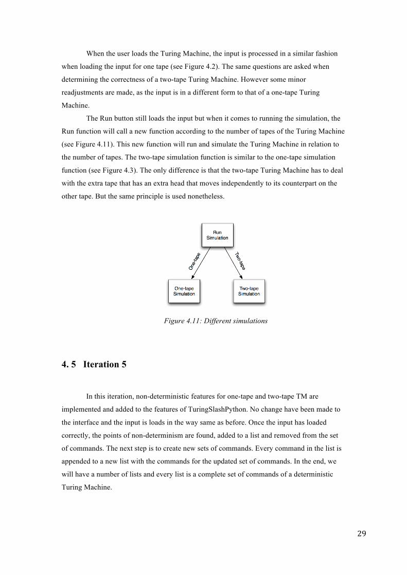
The Run button still loads the input but when it comes to running the simulation, the

Run function will call a new function according to the number of tapes of the Turing Machine

(see Figure 4.11). This new function will run and simulate the Turing Machine in relation to

the number of tapes. The two-tape simulation function is similar to the one-tape simulation

function (see Figure 4.3). The only difference is that the two-tape Turing Machine has to deal

with the extra tape that has an extra head that moves independently to its counterpart on the

other tape. But the same principle is used nonetheless.

Figure 4.11: Different simulations

4. 5 Iteration 5

In this iteration, non-deterministic features for one-tape and two-tape TM are

implemented and added to the features of TuringSlashPython. No change have been made to

the interface and the input is loads in the way same as before. Once the input has loaded

correctly, the points of non-determinism are found, added to a list and removed from the set

of commands. The next step is to create new sets of commands. Every command in the list is

appended to a new list with the commands for the updated set of commands. In the end, we

will have a number of lists and every list is a complete set of commands of a deterministic

Turing Machine.

30

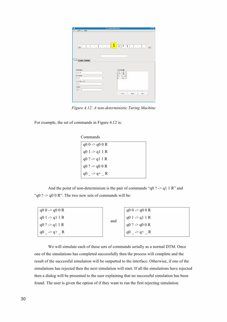
Figure 4.12: A non-deterministic Turing Machine

For example, the set of commands in Figure 4.12 is:

Commands

q0 0 -> q0 0 R

q0 1 -> q1 1 R

q0 ? -> q1 1 R

q0 ? -> q0 0 R

q0 _ -> q+ _ R

And the point of non-determinism is the pair of commands “q0 ? -> q1 1 R” and

“q0 ? -> q0 0 R”. The two new sets of commands will be:

q0 0 -> q0 0 R

q0 1 -> q1 1 R

q0 ? -> q1 1 R

q0 _ -> q+ _ R

and

q0 0 -> q0 0 R

q0 1 -> q1 1 R

q0 ? -> q0 0 R

q0 _ -> q+ _ R

We will simulate each of these sets of commands serially as a normal DTM. Once

one of the simulations has completed successfully then the process will complete and the

result of the successful simulation will be outputted to the interface. Otherwise, if one of the

simulations has rejected then the next simulation will start. If all the simulations have rejected

then a dialog will be presented to the user explaining that no successful simulation has been

found. The user is given the option of if they want to run the first rejecting simulation.

31

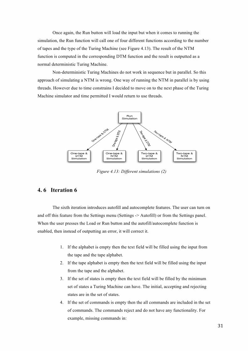
Once again, the Run button will load the input but when it comes to running the

simulation, the Run function will call one of four different functions according to the number

of tapes and the type of the Turing Machine (see Figure 4.13). The result of the NTM

function is computed in the corresponding DTM function and the result is outputted as a

normal deterministic Turing Machine.

Non-deterministic Turing Machines do not work in sequence but in parallel. So this

approach of simulating a NTM is wrong. One way of running the NTM in parallel is by using

threads. However due to time constrains I decided to move on to the next phase of the Turing

Machine simulator and time permitted I would return to use threads.

Figure 4.13: Different simulations (2)

4. 6 Iteration 6

The sixth iteration introduces autofill and autocomplete features. The user can turn on

and off this feature from the Settings menu (Settings -> Autofill) or from the Settings panel.

When the user presses the Load or Run button and the autofill/autocomplete function is

enabled, then instead of outputting an error, it will correct it.

1. If the alphabet is empty then the text field will be filled using the input from

the tape and the tape alphabet.

2. If the tape alphabet is empty then the text field will be filled using the input

from the tape and the alphabet.

3. If the set of states is empty then the text field will be filled by the minimum

set of states a Turing Machine can have. The initial, accepting and rejecting

states are in the set of states.

4. If the set of commands is empty then the all commands are included in the set

of commands. The commands reject and do not have any functionality. For

example, missing commands in:

32

a) A one-tape TM δ(q, X) = (r, Y, D), where ‘r’ is the rejecting state,

Y is X and the direction is right.

b) A two-tape TM δ(q, A, B) = (r, X, Y, D1, D2), where ‘r’ is the

rejecting state, X is A, Y is B and D1 and D2 are right.

5. Any duplicate values of a symbol in the alphabet will be removed.

6. If a symbol is in the tape but not in the alphabet then it will be added to the

alphabet.

7. Any duplicate values of a symbol in the tape alphabet will be removed.

8. If a symbol is in the alphabet but not in the tape alphabet then it will be added

to the tape alphabet.

9. Any duplicate values of a state in the set of states will be removed.

10. If the initial, accepting and rejecting states are missing from the set of states

then they will be appended to the set of states.

11. Missing commands will be appended to the set of commands (see step 4).

12. If a state in a command is not in the set of commands, then a message dialog

will give the user the option to delete the command, to include the state in the

set of states or to include the command in the set of commands. If the user

decides to append the state to the set of states then the user might need to

load the input again. If the user decides to keep the command, then he/she

can correct the mistake manually.

13. If the first value in a command is a halting state then a message dialog will

give the user the option to delete the command or to include it in the set of

commands. If the user decides to keep the command, then he/she can correct

the mistake manually.

14. If a symbol in a command is not in the tape alphabet, then a message dialog

will give the user the option to delete the command, to include the symbol in

the tape alphabet or to include the command in the set of commands. If the

user decides to append the symbol to the tape alphabet then the user might

need to load the input again. If the user decides to keep the command, then

he/she can correct the mistake manually.

15. If the third value of a one-tape command or the forth value of a two-tape

command is not the transition symbol then a message dialog will give the

user the option to correct the mistake, to delete the command or to include it

in the set of commands. If the user decides to keep the command, then he/she

can correct the mistake manually.

33

16. If an invalid direction is given then a message dialog will give the user the

option to delete the command or to include it in the set of commands. If the

user decides to keep the command, then he/she can correct the mistake

manually.

The aim of the autofill/autocomplete function is to help correct possible mistakes

anyone who is new to Turing Machines might make. However, it is not only aimed at

beginners, anyone can use the autofill/autocomplete function as a shortcut to filling in the

input of a Turing Machine.

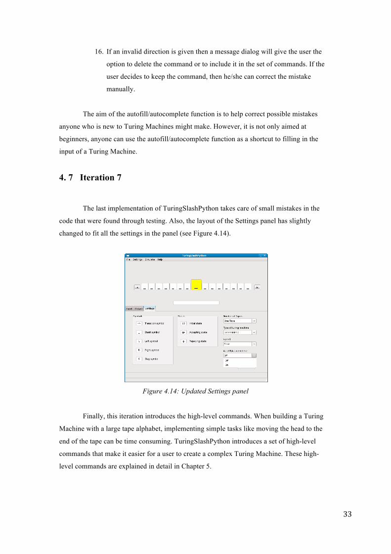
4. 7 Iteration 7

The last implementation of TuringSlashPython takes care of small mistakes in the

code that were found through testing. Also, the layout of the Settings panel has slightly

changed to fit all the settings in the panel (see Figure 4.14).

Figure 4.14: Updated Settings panel

Finally, this iteration introduces the high-level commands. When building a Turing

Machine with a large tape alphabet, implementing simple tasks like moving the head to the

end of the tape can be time consuming. TuringSlashPython introduces a set of high-level

commands that make it easier for a user to create a complex Turing Machine. These high-

level commands are explained in detail in Chapter 5.

34

4. 8 Conclusion

TuringSlashPython is aimed at people who are new to Turing Machines. It is assumed

that the users have made some mistakes and the error will be outputted or corrected. This

results in long loading times for large Turing Machine. Other Turing Machine simulators like

JFlap assume that the input given by the user is correct. See Appendix D for examples on how

TuringSlashPython works in practice.

35

Chapter 5: High-level commands

5. 1 Introduction

What makes TuringSlashPython unique compared to other Turing Machine

simulators are the high-level commands that make it easier for a user to create a complex

Turing Machine. When building a Turing Machine with a large tape alphabet, implementing

even the simplest task, for example moving the head to the end of the tape, can be time

consuming. A careful combination of high-level commands and the autofill function could

decrease the time needed to create a complex Turing Machine. A number of constraints are

given for every high-level command. These arguments act as variables that will be added to

the input if the autocorrect function is on. You can find the translations of every high-level

command with examples in Appendix E.

5. 2 High-level commands for one tape

5. 2. 1 The ‘go2start(q0, q1)’ command

This high-level command moves the head to the leftmost cell containing a non-black

symbol when in the state ‘q0’ and enters ‘q1’ once completed.

go2start(q0, q1) translates to:

q0 b q1 b R where ‘b’ is the blank symbol

q0 k q0 k L ∀ k ∈ Γ \ {‘b’}

Constraints

The tape input must be surrounded by blank symbols and there must not be a blank symbol within the

string. The arguments ‘q0’ and ‘q1’ must not be the same. The states ‘q0’ and ‘q1’ must be in the set of

states.

36

5. 2. 2 The ‘go2end(q0, q1)’ command

This high-level command moves the head to the rightmost cell containing a non-black

symbol when in the state ‘q0’ and enters ‘q1’ once completed.

go2end(q0, q1) translates to:

q0 b q1 b L where ‘b’ is the blank symbol

q0 k q0 k R ∀ k ∈ Γ \ {‘b’}

Constraints



states.

5. 2. 3 The ‘add2start(q0, q1, a)’ command

This high-level command moves the head to the leftmost cell containing a non-black

symbol when in the state ‘q0’ adds the symbol ‘a’ to the start and enters ‘q1’ once completed.

Constraints


string. The arguments ‘q0’ and ‘q1’ must not be the same. The symbol ‘a’ must be in the tape alphabet.

The states ‘q0’ and ‘q1’ must be in the set of states.

5. 2. 4 The ‘add2end(q0, q1, a)’ command

This high-level command moves the head to the rightmost cell containing a non-black

symbol when in the state ‘q0’ adds the symbol ‘a’ to the end and enters ‘q1’ once completed.

Constraints The tape input must be surrounded by blank symbols and there must not be a blank symbol within the


states. The symbol ‘a’ must be in the tape alphabet.

37

5. 2. 5 The ‘find(q0, q1, q2, a, D)’ command

This high-level command finds the first occurrence of the symbol ‘a’ when the state

is ‘q0’. If the symbol is found, the head enters the state ‘q1’ else the head enters ‘q2’. The

head will go in the direction ‘D’. If the symbol is not found then the head will move into the

opposite direction, “ D’ “. The symbol found will be the first occurrence nearest to the

position of the head when the state is ‘q0’ but might not be the first occurrence of the symbol

‘a’ in the whole of the string.

Constraints


string. The states ‘q0’, ‘q1’ and ‘q2’ must be in the set of states. The arguments ‘q0’, ‘q1’ and ‘q2’

must not be the same. The symbol ‘a’ must be in the tape alphabet. ‘D’ must be a valid direction.

5. 2. 6 The ‘replace(q0, q1, q2, a, b, D)’ command

This high-level command replaces the first occurrence of the symbol ‘a’ with the

symbol ‘b’, when the state is ‘q0’. If the symbol is found, the head enters the state ‘q1’ else

the head enters ‘q2’. The head will go in the direction ‘D’. If the symbol is not found then the

head will move into the opposite direction, “ D’ “. The symbol found will be the first

occurrence nearest to the position of the head when the state is ‘q0’ but might not be the first

occurrence of the symbol ‘a’ in the whole of the string.

Constraints


string. The states arguments ‘q0’, ‘q1’ and ‘q2’ must not be the same. The symbol arguments ‘a’ and

‘b’ must not be the same. The states ‘q0’, ‘q1’ and ‘q2’ must be in the set of states. The symbols ‘a’

and ‘b’ must be in the tape alphabet. ‘D’ must be a valid direction.

5. 2. 7 The ‘replaceall(q0, q1, q2, a, b)’ command

This high-level command replaces all occurrences of the symbol ‘a’ with ‘b’, when

the state is ‘q0’. The head will go to the start of the string and the state changes to ‘r’. By

going to the start of the string, we ensure that we replace all the symbols ‘a’. Once in state ‘r’,

38

if the symbol ‘1’ is found, the state changes to ‘ra’ and the symbol is replaced with the

symbol ‘a’, otherwise the head enters the state ‘q2’ and moves left. If the head is in the state

‘ra’ then we know that there is at least one occurrence of the symbol ‘a’. So the head can

continue replacing the symbols. Once the head is at the end of the string, all occurrences of

the symbol have been replaced; the head enters the state ‘q1’ and moves left.

Constraints



‘b’ must not be the same. The states ‘q0’, ‘q1’ and ‘q2’ must be in the set of states. The symbols ‘a’

and ‘b’ must be in the tape alphabet.

5. 2. 8 The ‘remove(q0, q1, a)’ command

This high-level command removes all occurrences of the symbol ‘a’, when the state is

‘q0’. The head will go to the start of the string and the state changes to ‘st’. By going to the

start of the string, we ensure that we remove all the symbols ‘a’. Once in state ‘st’, if the

symbol ‘a’ is found, the state changes to ‘re’, otherwise the head enters the state ‘q1’ and

moves left. If the state is ‘re’, the head will go to the start of the tape in order to shift the tape

by one cell to the right, thus overwriting the symbol ‘a’. Once the symbol ‘a’ has been

replaced by the symbol to its left, the head will enter the state ‘st’ and this process loops until

all occurrences of the symbol ‘a’ have been removed. When shifting the tape to the right, the

head has to ‘remember’ the symbol to the left of the current position of the head. This is done

through a state. ‘rwk’ is a state that indicates the previous symbol. For every k ∈Γ there is a

state ‘rwk’ and the symbol ‘k’ is remembered through the state ‘rwk’.

Constraints



states. The symbol ‘a’ must be in the tape alphabet.

5. 2. 9 The ‘copy(q0, q1, #, %)’ command

This high-level command copies the string between the ‘#’ symbols to a new location

between the ‘%’ symbols. The head will copy every symbol to the new location. When a

symbol s is copied, it is replaced by s’, so we know which cells have been copied. This

39

assures us that the same cell will not be copied again. These new symbols are added to the

tape alphabet. The set of the new symbols is denoted by Γ’. We define the function f so that

f(s) = s’, where s ∈ ( Γ \ ( {‘#’, ‘%’} ∪ Γ’ )) ∧ s’ ∈ Γ’.

The copy starts when the head is in the state ‘q0’. The head moves left until it finds

the first ‘#’ and then moves right to start reading the symbols between the ‘#’ symbols. The

head enters ‘st’ when the first symbol ‘#’ is found.

The head will ‘remember’ the symbol it scans through the state. Every symbol ‘k’ in

Γ \ ( {‘#’, ‘%’} ∪ Γ’ ) is connected to a state ‘cpk’. This state ‘memorises’ the symbol ‘k’ that

it scanned. If ‘#’ is scanned when the state is ‘st’ then ‘end’ is entered. This state denotes the

end of the string that is being copied.

When the state is ‘cpk’, the head will go right until the symbol scanned is the ‘%’

symbol and the state will change to ‘cpik’. The states ‘cpk’ and ‘cpik’ are connected to the

symbol ‘k’. However, when the state is ‘cpik’, the Turing Machine knows that the head has

passed the first ‘%’ symbol. The head will write the symbol ‘k’ when the symbol scanned is a

‘%’ or a blank symbol. The second ‘%’ symbol will be overwritten by the first symbol to be

copied. This is not a problem as when the state is ‘end’; the ‘%’ symbol is added to the end of

the new string.

When the symbol ‘k’ has been copied in the new location, the state changes to ‘re’, In

this state, the head will go left until it scans a symbol k’ ∈ Γ’. This is the symbol that was last

copied and any symbol to the right has been already copied. The head will go right to the next

symbol to be copied. The state ‘st’ is entered and this computation loops.

Eventually the string will have been copied in the new location. The next symbol the

head scans is the ‘#’ symbol at the end of the string and enters the ‘end’ state. The head will

go right until the symbol scanned is the ‘%’ symbol and the state will change to ‘endi’. The

state ‘endi’ works like the state ‘cpik’ but instead of adding the symbol ‘k’ to the end of the

new string, it adds the ‘%’ symbol that was overwritten.

Once that is done, all that is left to do is to go back to the original string and to

convert every symbol s’ ∈ Γ’ back to its original form. We define the function g so that

g(s’) = s, where s’ ∈ Γ’ ∧ s ∈ ( Γ \ ( {‘#’, ‘%’} ∪ Γ’ )). The head will enter the state ‘cl’. In

this state, the head goes left until it finds the ‘#’ symbol. Then the state will change to ‘cli’.

The head will convert every symbol s’ back to its original form. When the head scans the

other ‘#’ symbol, the state will change to ‘q1’, the head will move right and the process of

copying the string has completed.

Constraints


40

string. The string to be copied must have the symbol ‘#’ at the beginning and at the end of the string.

There must be at least one ‘%’ symbol to the right of the string to be copied. There must not be another

string to the right of the ‘%’ symbols. The symbols in Γ’ must not be in the original tape alphabet. The

state arguments ‘q0’ and ‘q1’ must not be the same. The symbol arguments ‘#’ and ‘%’ must not be the

same. The states ‘q0’ and ‘q1’ must be in the set of states. The symbols ‘#’ and ‘%’ must be in the tape

alphabet. The head should be between the symbols ‘#’ when the state is ‘q0’.

5. 2. 10 The ‘compare(q0, q1, q2, #, %)’ command

This high-level command will compare two strings. The first string is between ‘#’

symbols and the second one, to the right of the first, is between ‘%’ symbols. The head will

replace the first symbol s in the first string with s’. These new symbols are added to the tape

alphabet. The set of the new symbols is denoted by Γ’. We define the function f so that f(s) =

s’, where s ∈ ( Γ \ ( {‘#’, ‘%’} ∪ Γ’ )) ∧ s’ ∈ Γ’. The symbol s is ‘remembered’ through the

state and is compared with the first possible symbol in the second string. This process will

loop until an error is found; otherwise the strings are the same.

Once the state is ‘q0’, the head will go left until the beginning of the first string is

found. Then the head enters the state ‘st’. Now the head will scan the first symbol s in the first

string, replace it with s’ and ‘memorise’ it through the state, ‘cmk’.

The head will ‘remember’ the symbol it scans through the state. Every symbol ‘k’ in

Γ \ ( {‘#’, ‘%’} ∪ Γ’ ) is connected to a state ‘cmk’. This state ‘memorises’ the symbol ‘k’

that it scanned. If ‘#’ is scanned when the state is ‘st’ then ‘end’ is entered. This state denotes

the end of the first string.

The head will go right until it finds the ‘%’ symbol; this is the start of the second

string. The head will enter the state ‘cmik’. The states ‘cmk’ and ‘cmik’ are connected to the

symbol ‘k’. However, when the state is ‘cmik’, the Turing Machine knows that the head has

passed the first ‘%’ symbol. If the state is ‘cmik’, the head will skip any symbol that has

already been compared. Once the head scans a cell that hasn’t been inspected, it will compare

it to the symbol ‘k’ from the first string.

If the comparison is correct, the symbol s will be replaced by the symbol s’ and the

head will enter the state ‘re’. The head will go left until it finds the ‘#’ symbol at the end of

the first string. The state will change to ‘rei’. In this state, the head will go left until it finds

the last symbol it compared in the first string, k’ ∈ Γ’. The head will enter the state ‘st’ and

will move right.

Unless an error is found, the next cell to be compared will be at the end of the first

41

string containing the ‘#’ symbol. So the head will enter the ‘end’ state and will move right

until it finds the start of the second string. The state ‘endi’ is reached when the head has

scanned the ‘%’ symbol at the beginning of the second string.

The head will find the first cell that has not been compared. The symbol in the cell

should be the second ‘%’ symbol at the end of the second string; otherwise the strings have

different lengths. If the strings are the same, then the head enters the state ‘acc’. In this state,

the head will move left converting all the symbols s’ ∈ Γ’ back to their original form,

s ∈ Γ \ ( {‘#’, ‘%’} ∪ Γ’ ). We define the function g so that g(s’) = s, where s’ ∈ Γ’ ∧

∧ s ∈ ( Γ \ ( {‘#’, ‘%’} ∪ Γ’ )).

The head will continue to do this until it scans the symbol ‘#’ at the end of the first

string. The head will enter the state ‘acci’ and will continue to move left. The state ‘acci’ is

similar to ‘acc’, however the head will convert the symbols s’ ∈ Γ’ in the first string, back to

their original form with the use of the function g. The head will continue to do this until it

reaches the symbol ‘#’ at the beginning of the first string. The head will enter the state ‘q1’

and will move right and the comparison will complete successfully.

If at any point the comparison is incorrect, the head will enter the state ‘rej’. Just like

the state ‘acc’, ‘rej’ will convert all the symbols s’ ∈ Γ’ in the second string, back to their

original form.

The head will continue to move left until the symbol ‘#’ at the end of the first string

has been scanned. The head will enter the state ‘reji’. The state ‘reji’ is similar to the state

‘acci’, however since an error was found, there is a possibility that there is a cell that has not

been compared and the symbol within has not been converted. Once the head is in the state

‘reji’ will just skip those cells and will move left. The head will continue moving along the

first string until it scans the ‘#’ symbol at the beginning of the first string. The head will enter

the state ‘q2’ and the comparison with terminate unsuccessfully.

Constraints


string. The first string to be compared must have the symbol ‘#’ at the beginning and at the end of the

string. The second string to be compared must have the symbol ‘%’ at the beginning and at the end of

the string. The second string must be at the right of the first string. The symbols in Γ’ must not be in

the original tape alphabet. The state arguments ‘q0’, ‘q1’ and ‘q2’ must not be the same. The symbol

arguments ‘#’ and ‘%’ must not be the same. The states ‘q0’, ‘q1’ and ‘q2’ must be in the set of states.

The symbols ‘#’ and ‘%’ must be in the tape alphabet. The head should be between the symbols ‘#’

when the state is ‘q0’.

42

5. 3 High-level commands for two tapes

5. 3. 1 The ‘go2start(q0, q1)’ command

This high-level command moves both heads to the leftmost cell containing a non-

black symbol (see Sections 5.2.1 and E.2.1).


q0 b b q1 b b R R where ‘b’ is the blank symbol

q0 k n q0 k n L L ∀ (k, n) ∈ Γ \ {(‘b’, ‘b’)} ∧ n ≠ ‘b’ ∧ k ≠ ‘b’

q0 k b q0 k b L S ∀ (k, ‘b’) ∈ Γ ∧ k ≠ ‘b’

q0 b k q0 b k S L ∀ (‘b’, k) ∈ Γ ∧ k ≠ ‘b’

Constraints



states.

5. 3. 2 The ‘go2start1(q0, q1)’ and ‘go2start2(q0, q1)’ commands

The command ‘go2start1’ (see Section E.2.2) moves only the head on tape one. The

command ‘go2start2’ (see Section E.2.3) moves only the head on tape two. Both commands

are the same as ‘go2start’ for one tape (see Section 5.2.1).

go2start1(q0, q1) translates to:

q0 b n q1 b n R S ∀ (‘b’, n) ∈ Γ, where ‘b’ is the blank symbol

q0 k n q0 k n L S ∀ (k, n) ∈ Γ ∧ k ≠ ‘b’


q0 n b q1 n b S R ∀ (n, ‘b’) ∈ Γ, where ‘b’ is the blank symbol

q0 n k q0 n k S L ∀ (n, k) ∈ Γ ∧ k ≠ ‘b’

43

Constraints



states.

5. 3. 3 The ‘go2end(q0, q1)’ command

This high-level command moves both heads to the rightmost cell containing a non-

black symbol (see Sections 5.2.2 and E.2.4)

Constraints



states.

5. 3. 4 The ‘go2end1(q0, q1)’ and ‘go2end2(q0, q1) commands

The command ‘go2end1’ (see Section E.2.5) moves only the head on tape one. The

command ‘go2end2’ (see Section E.2.6) moves only the head on tape two. Both commands

are the same as ‘go2end’ for one tape (see Section 5.2.2).

Constraints



states.

5. 3. 5 The ‘add2start(q0, q1, a)’ command

This high-level command adds the symbol ‘a’ to the start of both strings (see Sections

5.2.3 and E.2.7).

Constraints


string. The arguments ‘q0’ and ‘q1’ must not be the same. The symbol (‘a’, ‘a’) must be in the tape

alphabet. The states ‘q0’ and ‘q1’ must be in the set of states.

44

5. 3. 6 The ‘add2start1(q0, q1, a)’ and ‘add2start2(q0, q1, a)’

commands

The command ‘add2start1’ (see Section E.2.8) moves only the head on tape one. The

command ‘add2start2’ (see Section E.2.9) moves only the head on tape two. Both commands

are the same as ‘add2start’ for one tape (see Section 5.2.3).

Constraints


string. The arguments ‘q0’ and ‘q1’ must not be the same. The symbol ‘a’ must be in the tape alphabet

of tape one, if the command is ‘add2start1’ or in the tape alphabet of tape two, if the command is

‘add2start2’. The states ‘q0’ and ‘q1’ must be in the set of states.

5. 3. 7 The ‘add2end(q0, q1, a)’ command

This high-level command adds the symbol ‘a’ to the end of both strings (see Sections

5.2.4 and E.2.10).

Constraints


string. The arguments ‘q0’ and ‘q1’ must not be the same. The symbol (‘a’, ‘a’) must be in the tape

alphabet. The states ‘q0’ and ‘q1’ must be in the set of states.

5. 3. 8 The ‘add2end1(q0, q1, a)’ and ‘add2end2(q0, q1, a)’

commands

The command ‘add2end1’ (see Section E.2.11) moves only the head on tape one. The

command ‘add2end2’ (see Section E.2.12) moves only the head on tape two. Both commands

are the same as ‘add2end’ for one tape (see Section 5.2.4).

Constraints


string. The arguments ‘q0’ and ‘q1’ must not be the same. The symbol ‘a’ must be in the tape alphabet

of tape one, if the command is ‘add2start1’ or in the tape alphabet of tape two, if the command is

‘add2start2’. The states ‘q0’ and ‘q1’ must be in the set of states.

45

5. 3. 9 The ‘find(q0, q1, q2, a, b, D)’ command

This high-level command finds the first occurrence of the symbol (‘a’, ‘b’) (see

Sections 5.2.5 and E.2.13).

Constraints



must not be the same. The symbol (‘a’, ‘b’) must be in the tape alphabet. ‘D’ must be a valid direction.

5. 3. 10 The ‘find1(q0, q1, q2, a, D)’ and ‘find2(q0, q1, q2, a, D)’

commands

The command ‘find1’ (see Section E.2.14) moves only the head on tape one. The

command ‘find2’ (see Section E.2.15) moves only the head on tape two. Both commands are

the same as ‘find’ for one tape (see Section 5.2.5).

Constraints



must not be the same. The symbol ‘a’ must be in the tape alphabet of the tape one if the command is

‘find1’ or in the tape alphabet of the tape two if the command is ‘find2’. ‘D’ must be a valid direction.

5. 3. 11 The ‘replace(q0, q1, q2, a, b, c, d, D)’ command

This high-level command replaces the first occurrence of the symbol (‘a’, ‘b’) with

(‘c’, ‘d’) (see Sections 5.2.6 and E.2.16).

Constraints


string. The states arguments ‘q0’, ‘q1’ and ‘q2’ must not be the same. The symbol arguments (‘a’, ‘b’)

and (‘c’, ‘a’) must not be the same. The states ‘q0’, ‘q1’ and ‘q2’ must be in the set of states. The

symbols (‘a’, ‘b’) and (‘c’, ‘d’) must be in the tape alphabet. ‘D’ must be a valid direction.

46

5. 3. 12 The ‘replace1(q0, q1, q2, 1, a, D)’ and

‘replace2(q0, q1, q2, 1, a, D)’ commands

The command ‘replace1’ (see Section E.2.17) moves only the head on tape one. The

command ‘replace2’ (see Section E.2.18) moves only the head on tape two. Both commands

are the same as ‘replace’ for one tape (see Section 5.2.6).

Constraints


string. The states arguments ‘q0’, ‘q1’ and ‘q2’ must not be the same. The symbol arguments ‘1’ and

‘a’ must not be the same. The states ‘q0’, ‘q1’ and ‘q2’ must be in the set of states. The symbols ‘1’

and ‘a’ must be in the tape alphabet of tape one if the command is ‘replace1’ or in the tape alphabet of

tape two if the command is ‘replace2’. ‘D’ must be a valid direction.

5. 3. 13 The ‘replaceall(q0, q1, q2, a, b, c, d)’ command

This high-level command replaces all occurrences of the symbol (‘a’, ‘b’) with the

symbol (‘c’, ‘d’) (see Sections 5.2.7 and E.2.19).

Constraints


string. The states arguments ‘q0’, ‘q1’ and ‘q2’ must not be the same. The symbol arguments (‘a’, ‘b’)

and (‘c’, ‘d’) must not be the same. The states ‘q0’, ‘q1’ and ‘q2’ must be in the set of states. The

symbols (‘a’, ‘b’) and (‘c’, ‘d’) must be in the tape alphabet.

5. 3. 14 The ‘replaceall1(q0, q1, q2, a, b)’ and

‘replaceall2(q0, q1, q2, a, b)’ commands

The command ‘replaceall1’ (see Section E.2.20) moves only the head on tape one.

The command ‘replaceall2’ (see Section E.2.21) moves only the head on tape two. Both

commands are the same as ‘replaceall’ for one tape (see Section 5.2.7).

Constraints



47

‘b’ must not be the same. The states ‘q0’, ‘q1’ and ‘q2’ must be in the set of states. The symbols ‘a' and

‘b’ must be in the tape alphabet of tape one if the command is ‘replaceall1’ or in the tape alphabet of

tape two if the command is ‘replaceall2’.

5. 3. 15 The ‘remove(q0, q1, a, b)’ command

This high-level command removes all occurrences of the symbol (‘a’, ’b’) (see

Sections 5.2.8 and E.2.22).

Constraints



states. The symbol (‘a’, ‘b’) must be in the tape alphabet.

5. 3. 16 The ‘remove1(q0, q1, a)’ and ‘remove2(q0, q1, a)’

commands

The command ‘remove1’ (see Section E.2.23) moves only the head on tape one. The

command ‘remove2’ (see Section E.2.24) moves only the head on tape two. Both commands

are the same as ‘remove’ for one tape (see Section 5.2.8).

Constraints



states. The symbol ‘a’ must be in the tape alphabet of tape one if the command is ‘remove1’ or in the

tape alphabet of tape two if the command is ‘remove2’.

5. 3. 17 The ‘copy(q0, q1, #, %)’ command

This high-level command copies the string between the ‘#’ symbols to a new location

between the ‘%’ symbols (see Sections 5.2.9 and E.2.25)

Constraints


48






alphabet. The head should be between the symbols ‘#’ when the state is ‘q0’.

5. 3. 18 The ‘copy1(q0, q1, #, %)’ and ‘copy2(q0, q1, #, %)’

commands

The command ‘copy1’ (see Section E.2.26) moves only the head on tape one. The

command ‘copy2’ (see Section E.2.27) moves only the head on tape two. Both commands are

the same as ‘copy’ for one tape (see Section 5.2.9).

Constraints







alphabet of the corresponding tape. The head on the corresponding tape should be between the symbols

‘#’ when the state is ‘q0’.

5. 3. 19 The ‘compare(q0, q1, q2, #, %)’ command

The ‘compare’ high-level command is not supported for two tapes. If the user tries to

input this command, he/she is presented with an error dialog explaining their mistake and

suggesting an alternative way of comparing both tapes by using the ‘compare1’ and

‘compare2’ high-level commands.

49

5. 3. 20 The ‘compare1(q0, q1, q2, #, %)’ and

‘compare2(q0, q1, q2, #, %)’ commands

The command ‘compare1’ (see Section E.2.28) moves only the head on tape one. The

command ‘compare2’ (see Section E.2.29) moves only the head on tape two. Both commands

are the same as ‘compare’ for one tape (see Section 5.2.10).

Constraints


string. The first string to be compared must have the symbol ‘#’ at the beginning and at the end of the

string. The second string to be compared must have the symbol ‘%’ at the beginning and at the end of

the string. The second string must be at the right of the first string. The symbols in Γ’ must not be in

the original tape alphabet. The state arguments ‘q0’, ‘q1’ and ‘q2’ must not be the same. The symbol

arguments ‘#’ and ‘%’ must not be the same. The states ‘q0’, ‘q1’ and ‘q2’ must be in the set of states.

The symbols ‘#’ and ‘%’ must be in the tape alphabet. The head on the corresponding tape should be

between the symbols ‘#’ when the state is ‘q0’.

50

Chapter 6: Evaluation

6. 1 Introduction

The evaluation of this project is split into three parts:

1. Student Feedback

2. TuringSlashPython Evaluation

3. Comparison with the JFlap Turing Machine simulator

6. 2 User Feedback

Third year students of the School of Computing of the University of Leeds were

asked to go through a tutorial that introduced them to TuringSlashPython and its

features. Once they completed the tutorial, the students were asked to fill in a feedback

form that focused on their experience with TuringSlashPython. The tutorial was aimed

at students who have some prior knowledge of Turing Machines and who attended the

COMP3930 – “Complexity & Approximation” module in which Turing Machines were

introduced. You can find the tutorial in Appendix G with the completed feedback forms.

Out of the eighteen students who took the COMP3930 module (excluding

myself), nine completed the tutorial and the filled in the feedback form.

Question 1: Is it easy to start the program? Yes (9), No (0)

Question 2: Is the user interface easy to understand? Yes (8), No (1)

Question 3: Is it easy to navigate through the program? Yes (9), No (0)

Question 4: Is useful feedback offered if something goes wrong? Yes (8), No(1)

Question 5: Is this program relevant to your programme of studies? Yes (9), No (0)

Question 6: Did you find TuringSlashPython useful? Yes (9), No (0)

Question 7: Did you find the high-‐level commands helpful? Yes (9), No (0)

Question 8: Would you use TuringSlashPython as support for assignments

involving Turing Machines? Yes (8), No (1)

51

Question 9: Would you recommend TuringSlashPython to somebody new to

Turing Machines? Yes (9), No (0)

Question 10: Have you ever used another Turing Machine simulator? Yes (4), No (5)

Question 11: If yes, then which one? JFlap (4), Other (0)

Question 12: Which simulator would you use in the future?

TuringSlashPython (8), JFlap (1), Other (0)

Variety of comments from the feedback forms:

Form 2: “There is hidden functionality which is not obvious when using

from the start. Input options are quite restricted especially for 2 tape machine. Once you

make a mistake you are trapped with all the error messages (maybe those could be

flushed to some file or something). Overall it could be useful for beginers.”

Form 3: “The warning message dialog should not be the only indicator

of a warning. Put the warning in the output panel. Otherwise easy to use and useful high

level commands.”

Form 9: “I found the high level commands very helpfull and usefull. I

definitelly would have used this program to do my coursework and to fully understand

how turing machines work.”

My role in this part of the project evaluation was to observe and note the

students’ reactions to the program and to answer any questions they might have.

Overall, the students completed the tutorial with little or no help within 10 to 15

minutes. The majority commented that their understanding of Turing Machines had

improved and that the high-‐level commands were above their expectations. However,

one student (Form 2) did not find the error messages useful and did not understand

how the autofill/autocomplete function worked. The student did not have a good

understanding of Turing Machines and could not comprehend the mistakes made and

the error messages outputted. The student turned down help when it was offered

claiming that they understood the mistakes made. Finally, one student (Form 3)

commented that the message in the warning dialog should be included in the Output

panel. A warning in the simulation of a Turing Machine does not stop the simulation

from running. The reason why I did not implement this was because I wanted to have a

minimal output in the Output panel.

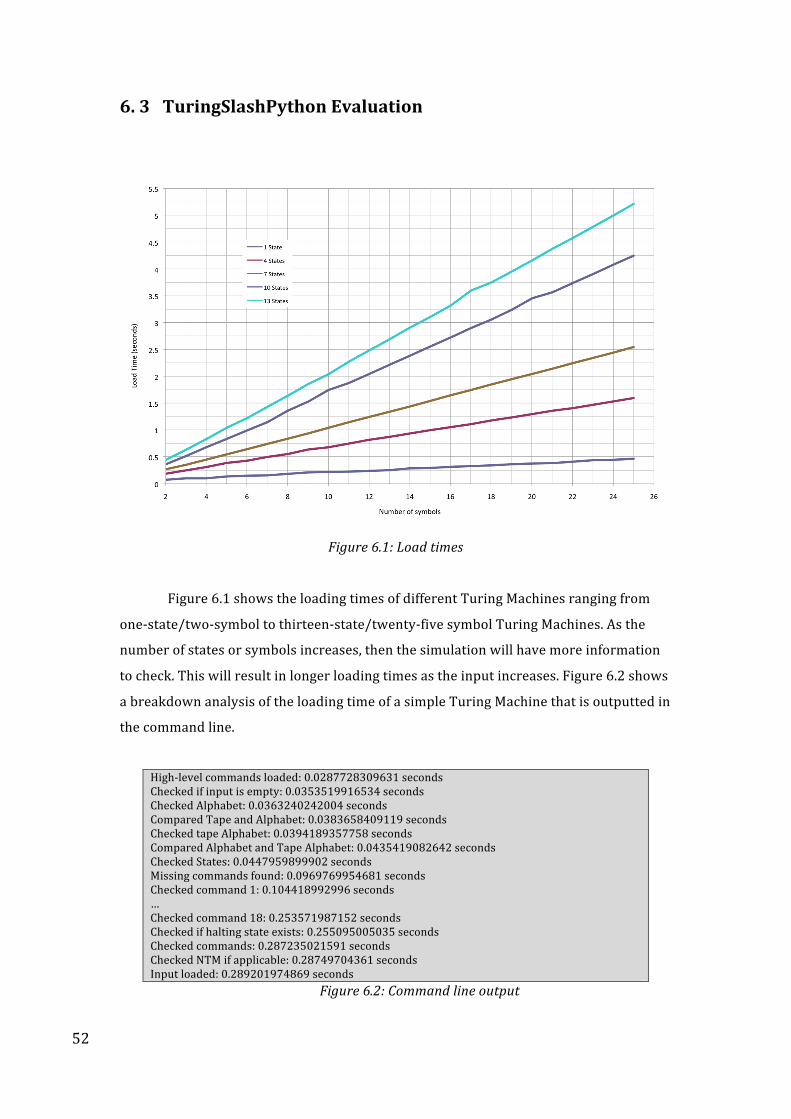
52

6. 3 TuringSlashPython Evaluation

Figure 6.1: Load times

Figure 6.1 shows the loading times of different Turing Machines ranging from

one-‐state/two-‐symbol to thirteen-‐state/twenty-‐five symbol Turing Machines. As the

number of states or symbols increases, then the simulation will have more information

to check. This will result in longer loading times as the input increases. Figure 6.2 shows

a breakdown analysis of the loading time of a simple Turing Machine that is outputted in

the command line.

High-‐level commands loaded: 0.0287728309631 seconds Checked if input is empty: 0.0353519916534 seconds Checked Alphabet: 0.0363240242004 seconds Compared Tape and Alphabet: 0.0383658409119 seconds Checked tape Alphabet: 0.0394189357758 seconds Compared Alphabet and Tape Alphabet: 0.0435419082642 seconds Checked States: 0.0447959899902 seconds Missing commands found: 0.0969769954681 seconds Checked command 1: 0.104418992996 seconds … Checked command 18: 0.253571987152 seconds Checked if halting state exists: 0.255095005035 seconds Checked commands: 0.287235021591 seconds Checked NTM if applicable: 0.28749704361 seconds Input loaded: 0.289201974869 seconds

Figure 6.2: Command line output

53

If the input has loaded successfully then the simulation will start. Every

configuration by the simulator takes 0.0003 to 0.0006 seconds to be generated. So for

most Turing Machines finding the result of the simulation is faster than checking the

validity of the input. A simple Turing Machine that checks if a string that consists of 0’s

and 1’s is a palindrome takes 0.45 to 0.6 seconds to load. While running this Turing

Machine on a palindrome that consists of 42 0’s and 1’s takes 0.42 to 0.43 seconds to

complete (946 configurations).

When a user runs the same simulation twice, the input is checked twice. If the

simulation is correct and no change has been made in the input after the first simulation

then the input should not be checked for validity the second time. Unfortunately,

TuringSlashPython will always check the correctness of the input and due to time

restraints I was not able to produce an improved solution. The loading time of a Turing

Machines increases as the states and symbols increase (See Figure 6.1). This loading

time could be avoided if the same Turing Machine is simulated twice. For example, if a

user would like to run the same Turing Machine on two different tape inputs, then in the

second simulation only the tape input should be checked for correctness, thus reducing

the loading time dramatically. This can be achieved by saving the alphabet, the tape

alphabet, the set of states and the set of commands of a Turing Machine that has loaded

successfully. When the user loads or runs a second simulation, then if the current input

given is the same input as in the previous simulation, then the input should not be

checked, as TuringSlashPython knows that the input is correct.

Another issue with the simulator that was mentioned in one of the tutorial

sessions was the lack of a “Stop” button. Once the simulation has started it cannot be

stopped. If the input is loading or the actual simulation is running on the tape, the

interface will lock and the user cannot interact with it. This is why a “Stop” button does

not replace the “Run” button on the Input panel once the simulation has started. A

possible solution would be to use threads to split the simulating part from the interface

part of the program. By doing this, the user would be able to interact with the interface

while the simulation is running. The user would be allowed to stop the simulation using

the “Stop” button or to change the speed of the simulation.

High-‐level commands are translated very fast when the input is loaded. The

process of translating a high-‐level command is a small fraction of the overall loading

time. More complex high-‐level commands (see table 6.4) create more low-‐level

commands as more states and symbols are introduced. The translation of a complex

high-‐level command needs more time to complete, however this is still a small fraction

of the overall loading time, as more commands must be checked.

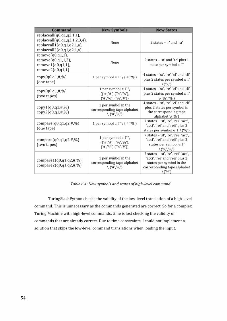
54

Command New Symbols New States replaceall(q0,q1,q2,1,a), replaceall(q0,q1,q2,1,2,3,4), replaceall1(q0,q1,q2,1,a), replaceall2(q0,q1,q2,1,a)

None 2 states – ‘r’ and ‘ra’

remove(q0,q1,1), remove(q0,q1,1,2), remove1(q0,q1,1), remove2(q0,q1,1)

None 2 states – ‘st’ and ‘re’ plus 1 state per symbol ∈ Γ

copy(q0,q1,#,%) (one tape)

1 per symbol ∈ Γ \ {‘#’,’%’}

4 states – ‘st’, ‘re’, ‘cl’ and ‘cli’ plus 2 states per symbol ∈ Γ

\{‘%’}

copy(q0,q1,#,%) (two tapes)

1 per symbol ∈ Γ \ {(‘#’,’#’),(’%’,’%’), (‘#’,’%’),(’%’,’#’)}

4 states – ‘st’, ‘re’, ‘cl’ and ‘cli’ plus 2 states per symbol ∈ Γ

\{‘%’, ‘%’}

copy1(q0,q1,#,%) copy2(q0,q1,#,%)

1 per symbol in the corresponding tape alphabet

\ {‘#’,’%’}

4 states – ‘st’, ‘re’, ‘cl’ and ‘cli’ plus 2 states per symbol in the corresponding tape

alphabet \{‘%’}

compare(q0,q1,q2,#,%) (one tape)

1 per symbol ∈ Γ \ {‘#’,’%’}

7 states – ‘st’, ‘re’, ‘rei’, ‘acc’, ‘acci’, ‘rej’ and ‘reji’ plus 2 states per symbol ∈ Γ \{‘%’}

compare(q0,q1,q2,#,%) (two tapes)

1 per symbol ∈ Γ \ {(‘#’,’#’),(’%’,’%’), (‘#’,’%’),(’%’,’#’)}

7 states – ‘st’, ‘re’, ‘rei’, ‘acc’, ‘acci’, ‘rej’ and ‘reji’ plus 2 states per symbol ∈ Γ

\{‘%’,‘%’}

compare1(q0,q1,q2,#,%) compare2(q0,q1,q2,#,%)

1 per symbol in the corresponding tape alphabet

\ {‘#’,’%’}

7 states – ‘st’, ‘re’, ‘rei’, ‘acc’, ‘acci’, ‘rej’ and ‘reji’ plus 2 states per symbol in the

corresponding tape alphabet \{‘%’}

Table 6.4: New symbols and states of high-level command

TuringSlashPython checks the validity of the low-‐level translation of a high-‐level

command. This is unnecessary as the commands generated are correct. So for a complex

Turing Machine with high-‐level commands, time is lost checking the validity of

commands that are already correct. Due to time constraints, I could not implement a

solution that skips the low-‐level command translations when loading the input.

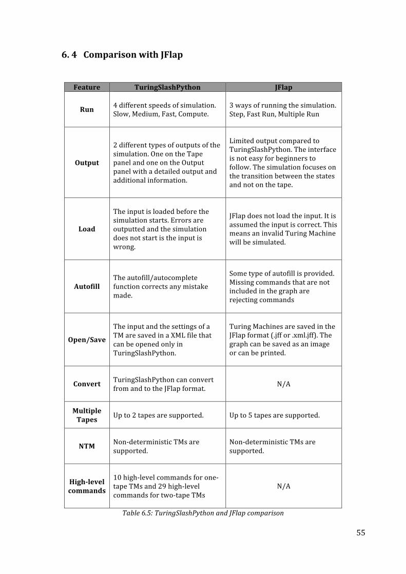
55

6. 4 Comparison with JFlap

Feature TuringSlashPython JFlap

Run

4 different speeds of simulation. Slow, Medium, Fast, Compute.

3 ways of running the simulation. Step, Fast Run, Multiple Run

Output

2 different types of outputs of the simulation. One on the Tape panel and one on the Output panel with a detailed output and additional information.

Limited output compared to TuringSlashPython. The interface is not easy for beginners to follow. The simulation focuses on the transition between the states and not on the tape.

Load

The input is loaded before the simulation starts. Errors are outputted and the simulation does not start is the input is wrong.

JFlap does not load the input. It is assumed the input is correct. This means an invalid Turing Machine will be simulated.

Autofill The autofill/autocomplete function corrects any mistake made.

Some type of autofill is provided. Missing commands that are not included in the graph are rejecting commands

Open/Save

The input and the settings of a TM are saved in a XML file that can be opened only in TuringSlashPython.

Turing Machines are saved in the JFlap format (.jff or .xml.jff). The graph can be saved as an image or can be printed.

Convert

TuringSlashPython can convert from and to the JFlap format.

N/A

Multiple Tapes

Up to 2 tapes are supported.

Up to 5 tapes are supported.

NTM

Non-‐deterministic TMs are supported.

Non-‐deterministic TMs are supported.

High-level commands

10 high-‐level commands for one-‐tape TMs and 29 high-‐level commands for two-‐tape TMs

N/A

Table 6.5: TuringSlashPython and JFlap comparison

56

References

[1] Turing, Alan M. “On Computable Numbers, with an Application to the

Entscheidungsproblem”. Proceedings of the London Mathematical Society, 1937, 2 (42),

230-265.

[2] Hopcroft, John E.; Rajeev Motwani and Ullman, Jeffrey D., 2000, Introduction to

Automata Theory, Languages, and Computation (2nd ed), Addison-Wesley Publishers

Limited.

[3] Jarvis, Jonathan and Lucas, Joan M. “Understanding the Universal Turing Machine: An

implementation in JFlap”. Journal of Computing Sciences in Colleges, 2008 23 (5), 180-

188.

[4] Duke University Department of Computer Science. JFlap [online]. 2010. [Accessed 29

January 2010]. Available from:

http://www.cs.duke.edu/csed/jflap/

[5] Rodger, Susan H. and Finley, Thomas W., 2006, JFlap: An Interactive Formal

Languages and Automata Package, Jones and Bartlett Publishers.

[6] Charvat, Jason, 2003, Project Management Methodologies: Selecting, Implementing,

and Supporting Methodologies and Processes for Projects, John Wiley & Sons, Inc.

[7] Agarwal, R. and Umphress, D, 2008. “Extreme programming for a single person team”. In

Proceedings of the 46th Annual Southeast Regional Conference on XX (Auburn,

Alabama, March 28 - 29, 2008). ACM-SE 46. ACM, New York, NY, 82-87.

[8] Sommerville, Ian, 2007, Software Engineering (8th edition), Addidon-Wesley Publishers

Limited.

[9] Humphrey, Watts S., 1996, Introduction to the Personal Software Process. Addison

Wesley Longman.

57

[10] Hodges, A. JavaScript Turing Machines [online]. 2010. [Accessed 29 January 2010].

Available from:

http://www.turing.org.uk/turing/scrapbook/tmjava.html

[11] SourceForge.net. Tuatara Turing Machine Simulator [online]. 2010. [Accessed 29

January 2010]. Available from:

http://sourceforge.net/projects/tuataratmsim/

[12] Britton, S. Turing Machine Simulator [online]. 2010. [Accessed 29 January 2010].

Available from:

http://ironphoenix.org/tril/tm/

[13] Buena Vista University. Turing Machine [online]. 2010. [Accessed 29 January 2010].

Available from:

http://web.bvu.edu/faculty/schweller/Turing/Turing.html

[14] Kennedy, J. Turing Machine Simulator [online]. 2010. [Accessed 29 January 2010].

Available from:

http://archives.math.utk.edu/software/msdos/miscellaneous/jkturing/.html

[15] Wittenberg University. A Turing Machine Simulator Program [online]. 2010. [Accessed

29 January 2010]. Available from:

http://www3.wittenberg.edu/bshelburne/Turing.htm

[16] Jones, Phil, 1998, Visual Basic: A Complete Course. Thomson Learning.

[17] Jones, Christopher A., 2002, Python & XML. O’Reilly.

58

Appendix A: Personal Reflection

I enjoyed developing this program as I was given the opportunity to turn something

theoretical into to something practical for the benefit of future students. I am pleased with the

end result and satisfied with how smoothly it went with no major barriers. I have never

worked on a project of this scale before and I felt the experience beneficial for future projects

I may come across. In the last three years, I have learnt valuable lessons that will stay with me

throughout my career, but though my life also.

When choosing a project, I carefully analysed the requirements of the projects that

that I found interesting and this allowed me to choose a project that I felt I could produce to

the highest level. On the downside, I had a few difficulties fitting everything in my schedule

over one semester. However, good understanding of the problem, choosing appropriate

methodologies and asking of help when stuck, made the task simpler.

A major part of my project was the evaluation. I chose my evaluation style before the

implementation of the program had finished. I had to postpone the evaluation for a later date

until I had completed the program with all the desirable features. Part of the evaluation

depended on user feedback. The task of convincing others to take some time to evaluate my

program turned to be trickier that what I expected as the majority of people where busy with

their own projects.

To conclude, I am happy with solution I developed, the skills that I have gained will

help me progress through my future career. Further skills I feel I have acquired throughout

my three years at the University of Leeds are both academic and social, from this I believe

that I have made the most of my student life, whilst trying to keep a balance between

university work and personal time. If I had to do the project again, I would have spent some

time improving the program based on the user feedback.

To future 3rd year students:

• Select a project that you are interested in.

59

• Plan your time schedule properly to avoid any disappointment. Set

milestones and do not miss deadlines. Keep a balance between work and

rest.

• Your background research is the cornerstone of your project. Fully

understanding the task in hand by researching the problem is the first step

to success.

• Keep detailed notes and write your progress in a dairy. These will come

in handy during your write-up.

• Don’t be afraid to ask questions. Your supervisor is there to point you in

the right direction when you get stuck.

• Start your write-up early to get feedback.

• Don’t forget to have fun!

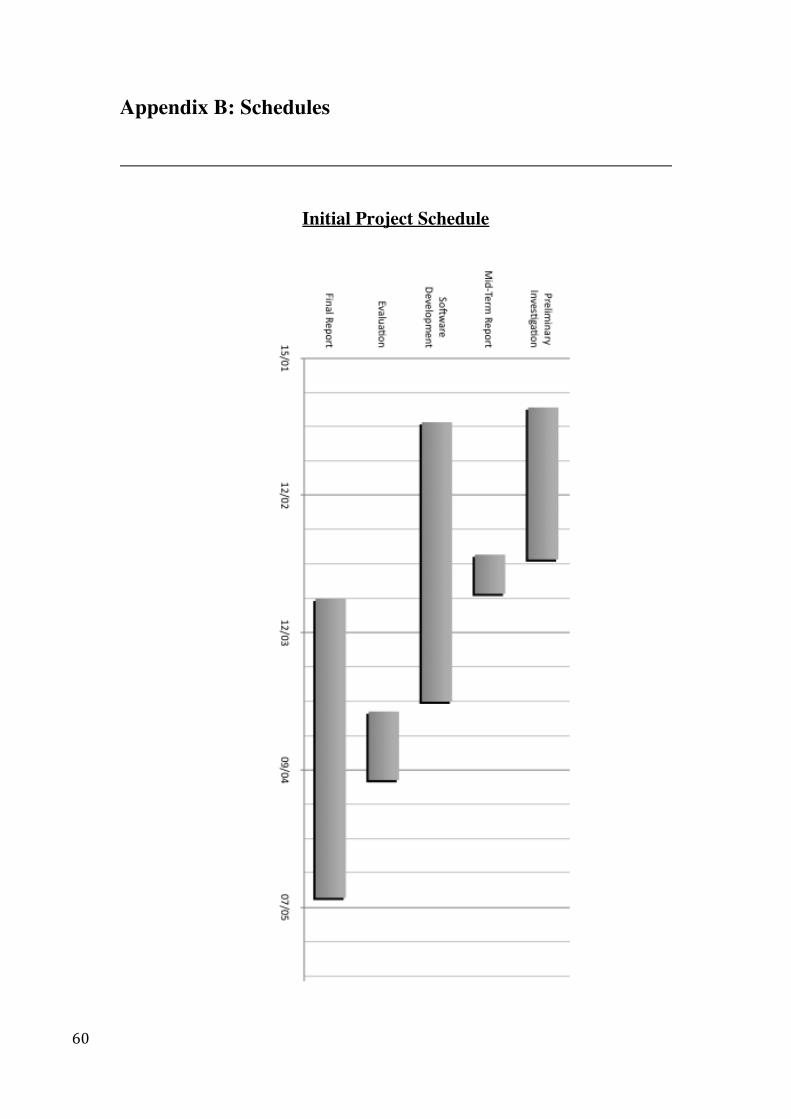
60

Appendix B: Schedules

Initial Project Schedule

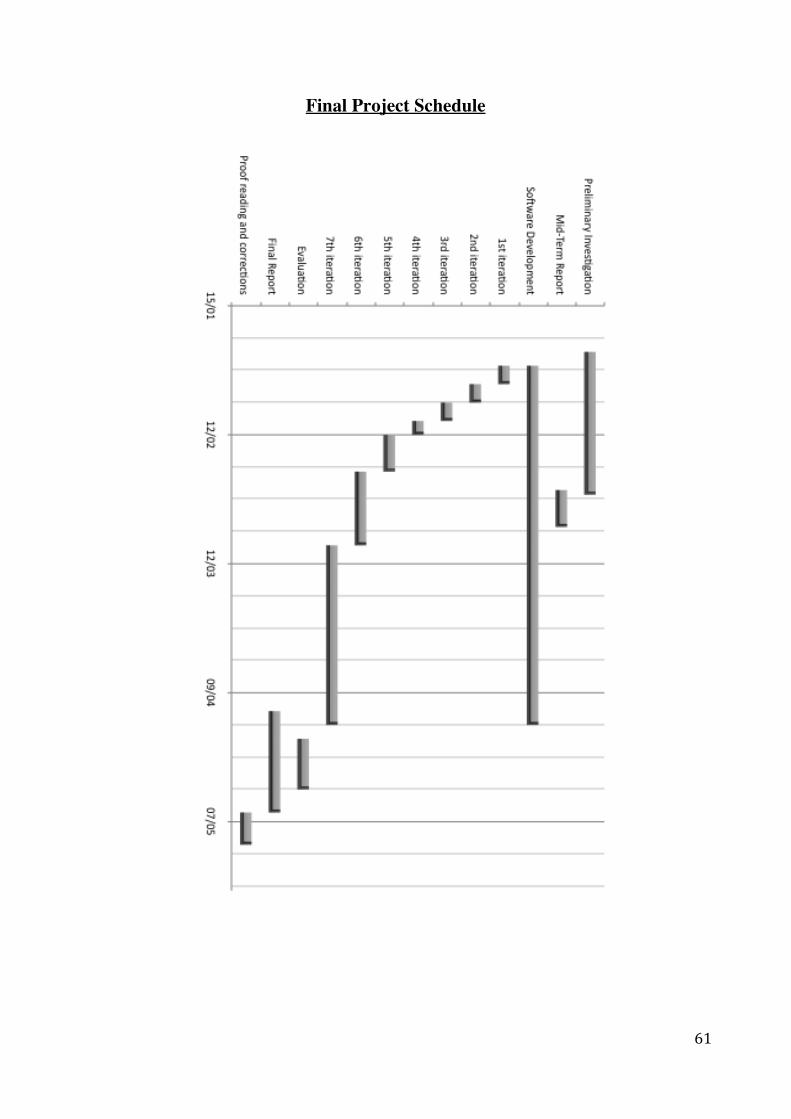
61

Final Project Schedule

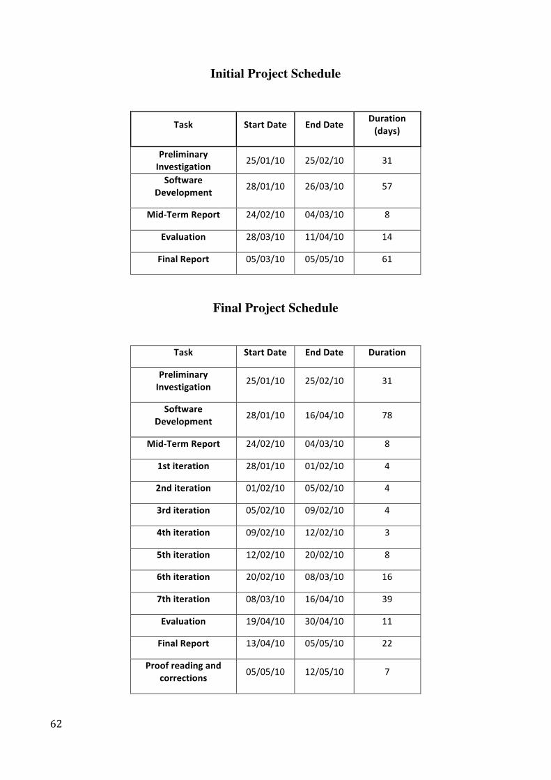
62

Initial Project Schedule

Task Start Date End Date Duration (days)

Preliminary Investigation

25/01/10 25/02/10 31

Software Development

28/01/10 26/03/10 57

Mid-‐Term Report 24/02/10 04/03/10 8

Evaluation 28/03/10 11/04/10 14

Final Report 05/03/10 05/05/10 61

Final Project Schedule

Task Start Date End Date Duration

Preliminary Investigation

25/01/10 25/02/10 31

Software Development

28/01/10 16/04/10 78

Mid-‐Term Report 24/02/10 04/03/10 8

1st iteration 28/01/10 01/02/10 4

2nd iteration 01/02/10 05/02/10 4

3rd iteration 05/02/10 09/02/10 4

4th iteration 09/02/10 12/02/10 3

5th iteration 12/02/10 20/02/10 8

6th iteration 20/02/10 08/03/10 16

7th iteration 08/03/10 16/04/10 39

Evaluation 19/04/10 30/04/10 11

Final Report 13/04/10 05/05/10 22

Proof reading and corrections

05/05/10 12/05/10 7

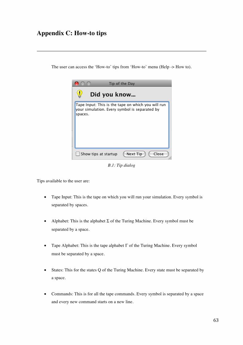
63

Appendix C: How-to tips

The user can access the ‘How-to’ tips from ‘How-to’ menu (Help -> How to).

B.1: Tip dialog

Tips available to the user are:

• Tape Input: This is the tape on which you will run your simulation. Every symbol is

separated by spaces.

• Alphabet: This is the alphabet Σ of the Turing Machine. Every symbol must be

separated by a space.

• Tape Alphabet: This is the tape alphabet Γ of the Turing Machine. Every symbol

must be separated by a space.

• States: This for the states Q of the Turing Machine. Every state must be separated by

a space.

• Commands: This is for all the tape commands. Every symbol is separated by a space

and every new command starts on a new line.

64

• Settings: You can change the settings of the Turing Machine simulator from the

Settings tab or the settings menu.

• Settings: Remember to press the Apply button if you are changing the settings from

the Settings tab.

• Load: The Load button checks if the input given is correct. If you make a mistake,

you will get an error message.

• Run: The Run button checks if the input given is correct and the runs the simulation.

If you make a mistake, you will get an error message and the simulation will not start.

• Symbols: The transition symbol is '->', the blank symbol is 'b', the left symbol is 'L',

the right symbol is 'R' and the stay symbol is 'S'. You can change all these symbols in

the Settings tab.

• States: The initial state is 'q0', the accepting state is 'q+' and the rejecting state is 'q-'.

You can change all these states in the Settings tab.

• Tape Input: If the number of tapes is 2 then the 1st symbol in the tape input is on tape

one, the 2nd symbol is on tape two, the 3rd is on tape one, the 4th is on tape two and

so on...

• Alphabet and Tape Alphabet: If the number of tapes is 2 then the 1st symbol belongs

to tape one, the 2nd symbol belongs to tape two, the 3rd belongs to tape one, the 4th

belongs to tape two and so on...

• Autofill: You can turn on the autofill / autocorrect function from the Settings tab or

from the Settings menu (Settings -> Autofill).

• Autofill: The autofill / autocorrect function will autofill any missing input and

corrects any reasonable mistake.

• High-level commands: High-level commands make it easier to create a more complex

Turing Machine.

65

• High-level commands: (One tape and two tapes) 'go2start(q0,q1)', 'go2end(q0,q1)',

'add2start(q0,q1,a)', add2end(q0,q1,a), copy(q0,q1,#,%), compare(q0,q1,q2,#,%)

• High-level commands: (One tape only) find(q0,q1,q2,1,D), replace(q0,q1,q2,1,a,D),

replaceall(q0,q1,q2,1,a), remove(q0,q1,1)

• High-level commands: (Two tapes only) go2start1(q0,q1), go2start2(q0,q1),

go2end1(q0,q1), go2end2(q0,q1), 'add2start1(q0,q1,a)','add2start2(q0,q1,a)',

add2end1(q0,q1,a), add2end2(q0,q1,a), find(q0,q1,q2,1,2,D), find1(q0,q1,q2,1,D),

find2(q0,q1,q2,1,D), replace(q0,q1,q2,1,2,3,4,D), replace1(q0,q1,q2,1,2,D),

replace2(q0,q1,q2,1,2,D), replaceall(q0,q1,q2,1,2,3,4), replaceall1(q0,q1,q2,1,a),

replaceall2(q0,q1,q2,1,a), remove(q0,q1,1,2), remove1(q0,q1,1), remove2(q0,q1,1)

• High-level commands: Note that commas and no spaces must separate the arguments

in the high-level commands.

• High-level commands: Make sure the autofill function is on before running a

complex high-level command.

• High-level commands: 'go2start(q0,q1)'. This high-level command moves the head

(or heads if the number of tapes is 2) to the start of the tape when in the state q0 and

enters q1 once completed (One tape and two tapes).

• High-level commands: 'go2start1(q0,q1)'. This high-level command moves the head

on tape one to the start of the tape when in the state q0 and enters q1 once completed

(Two tapes).

• High-level commands: 'go2start2(q0,q1)'. This high-level command moves the head

on tape two to the start of the tape when in the state q0 and enters q1 once completed

(Two tapes).

• High-level commands: 'go2end(q0,q1)'. This high-level command moves the head (or

heads if the number of tapes is 2) to the end of the tape when in the state q0 and


66

• High-level commands: 'go2end1(q0,q1)'. This high-level command moves the head

on tape one to the end of the tape when in the state q0 and enters q1 once completed

(Two tapes).

• High-level commands: 'go2end2(q0,q1)'. This high-level command moves the head

on tape two to the end of the tape when in the state q0 and enters q1 once completed

(Two tapes).

• High-level commands: 'add2start(q0,q1,1)'. This high-level command adds the

symbol 1 (or 1 1 if the number of tapes is 2) to the start of the tape when in the state

q0 and enters q1 once completed (One tape and two tapes).

• High-level commands: 'add2start1(q0,q1,1)'. This high-level command adds the

symbol 1 to the start of tape one when in the state q0 and enters q1 once completed

(Two tapes).

• High-level commands: 'add2start2(q0,q1,1)'. This high-level command adds the

symbol 1 to the start of tape two when in the state q0 and enters q1 once completed

(Two tapes).

• High-level commands: 'add2end(q0,q1,1)'. This high-level command adds the symbol

1 (or 1 1 if the number of tapes is 2) to the end of the tape when in the state q0 and


• High-level commands: 'add2end1(q0,q1,1)'. This high-level command adds the

symbol 1 to the end of tape one when in the state q0 and enters q1 once completed

(Two tapes).

• High-level commands: 'add2end2(q0,q1,1)'. This high-level command adds the

symbol 1 to the end of tape two when in the state q0 and enters q1 once completed

(Two tapes).

• High-level commands: 'find(q0,q1,q2,1,D)'. This high-level command moves the

head in direction D and finds the symbol 1 on the tape when in the state q0 and enters

q1 if found, otherwise it enters q2 (One tape).

67

• High-level commands: 'find(q0,q1,q2,1,2,D)'. This high-level command moves the

heads in direction D and finds the symbol 1 2 on the tape when in the state q0 and

enters q1 if found, otherwise it enters q2 (Two tapes).

• High-level commands: 'find1(q0,q1,q2,1,D)'. This high-level command moves the

head on tape one in direction D and finds the symbol 1 on tape one when in the state

q0 and enters q1 if found, otherwise it enters q2 (Two tapes).

• High-level commands: 'find2(q0,q1,q2,1,D)'. This high-level command moves the

head on tape two in direction D and finds the symbol 1 on tape two when in the state

q0 and enters q1 if found, otherwise it enters q2 (Two tapes).

• High-level commands: 'replace(q0,q1,q2,1,a,D)'. This high-level command moves the

head in direction D and replaces the symbol 1 on the tape with the symbol a when in

the state q0 and enters q1 if found, otherwise it enters q2 (One tape).

• High-level commands: 'replace(q0,q1,q2,1,2,3,4,D)'. This high-level command moves

the heads in direction D and replaces the symbol 1 2 on the tape with the symbol 3 4

when in the state q0 and enters q1 if found, otherwise it enters q2 (Two tapes).

• High-level commands: 'replace1(q0,q1,q2,1,a,D)'. This high-level command moves

the head on tape one in direction D and replaces the symbol 1 on tape one with the

symbol a when in the state q0 and enters q1 if found, otherwise it enters q2 (Two

tapes).

• High-level commands: 'replace2(q0,q1,q2,1,a,D)'. This high-level command moves

the head on tape two in direction D and replaces the symbol 1 on tape two with the

symbol a when in the state q0 and enters q1 if found, otherwise it enters q2 (Two

tapes).

• High-level commands: 'replaceall(q0,q1,q2,1,a)'. This high-level command replaces

all occurrences of the symbol 1 on the tape with the symbol a when in the state q0

and enters q1 once completed, otherwise it enters q2 (One tape).

68

• High-level commands: 'replaceall(q0,q1,q2,1,2,3,4)'. This high-level command

replaces all occurrences of the symbol 1 2 on the tape with the symbol 3 4 when in

the state q0 and enters q1 once completed, otherwise it enters q2 (Two tapes).

• High-level commands: 'replaceall1(q0,q1,q2,1,a)'. This high-level command replaces

all occurrences of the symbol 1 on tape one with the symbol a when in the state q0

and enters q1 once completed, otherwise it enters q2 (Two tapes).

• High-level commands: 'replaceall2(q0,q1,q2,1,a)'. This high-level command replaces

all occurrences of the symbol 1 on tape two with the symbol a when in the state q0

and enters q1 once completed, otherwise it enters q2 (Two tapes).

• High-level commands: 'remove(q0,q1,1)'. This high-level command removes all

occurrences of the symbol 1 on the tape when in the state q0 and enters q1 once

completed (One tape).

• High-level commands: 'remove(q0,q1,1,2)'. This high-level command removes all

occurrences of the symbol 1 2 on the tape when in the state q0 and enters q1 once

completed (Two tapes).

• High-level commands: 'remove1(q0,q1,1)'. This high-level command removes all

occurrences of the symbol 1 on tape one when in the state q0 and enters q1 once


• High-level commands: 'remove2(q0,q1,1)'. This high-level command removes all

occurrences of the symbol 1 on tape two when in the state q0 and enters q1 once


• High-level commands: 'copy(q0,q1,#,%)'. This high-level command copies the string

between the # to the location between the % and enters q1 once completed (One tape

and two tapes).

• High-level commands: 'copy1(q0,q1,#,%)'. This high-level command copies the

string between the # to the location between the % on tape one and enters q1 once


69

• High-level commands: 'copy2(q0,q1,#,%)'. This high-level command copies the

string between the # to the location between the % on tape two and enters q1 once


• High-level commands: 'compare(q0,q1,q2,#,%)'. This high-level command compares

the strings between the # and the % and enters q1 if correct, otherwise it enters q2

(One tape and two tapes).

• High-level commands: 'compare1(q0,q1,q2,#,%)'. This high-level command

compares the strings between the # and the % on tape one and enters q1 if correct,

otherwise it enters q2 (Two tapes).

• High-level commands: 'compare2(q0,q1,q2,#,%)'. This high-level command

compares the strings between the # and the % on tape two and enters q1 if correct,

otherwise it enters q2 (Two tapes).

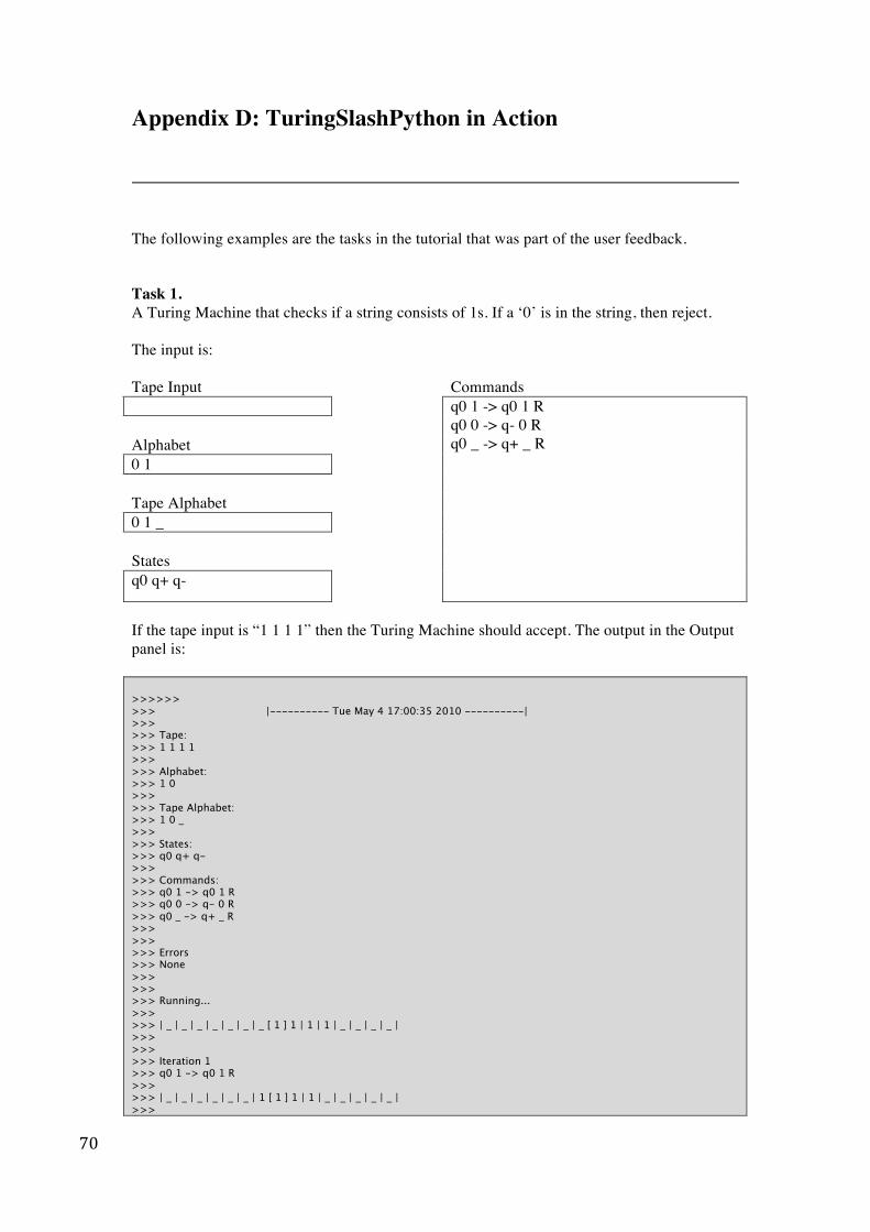
70

Appendix D: TuringSlashPython in Action

The following examples are the tasks in the tutorial that was part of the user feedback.

Task 1. A Turing Machine that checks if a string consists of 1s. If a ‘0’ is in the string, then reject. The input is: Tape Input Commands Alphabet 0 1 Tape Alphabet 0 1 _ States q0 q+ q-

q0 1 -> q0 1 R q0 0 -> q- 0 R q0 _ -> q+ _ R

If the tape input is “1 1 1 1” then the Turing Machine should accept. The output in the Output panel is: >>>>>> >>> |---------- Tue May 4 17:00:35 2010 ----------| >>> >>> Tape: >>> 1 1 1 1 >>> >>> Alphabet: >>> 1 0 >>> >>> Tape Alphabet: >>> 1 0 _ >>> >>> States: >>> q0 q+ q- >>> >>> Commands: >>> q0 1 -> q0 1 R >>> q0 0 -> q- 0 R >>> q0 _ -> q+ _ R >>> >>> >>> Errors >>> None >>> >>> >>> Running... >>> >>> | _ | _ | _ | _ | _ | _ | _ [ 1 ] 1 | 1 | 1 | _ | _ | _ | _ | >>> >>> >>> Iteration 1 >>> q0 1 -> q0 1 R >>> >>> | _ | _ | _ | _ | _ | _ | 1 [ 1 ] 1 | 1 | _ | _ | _ | _ | _ | >>>

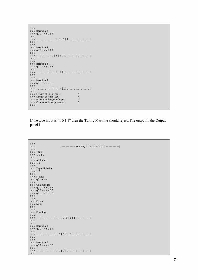
71

>>> >>> Iteration 2 >>> q0 1 -> q0 1 R >>> >>> | _ | _ | _ | _ | _ | 1 | 1 [ 1 ] 1 | _ | _ | _ | _ | _ | _ | >>> >>> >>> Iteration 3 >>> q0 1 -> q0 1 R >>> >>> | _ | _ | _ | _ | 1 | 1 | 1 [ 1 ] _ | _ | _ | _ | _ | _ | _ | >>> >>> >>> Iteration 4 >>> q0 1 -> q0 1 R >>> >>> | _ | _ | _ | 1 | 1 | 1 | 1 [ _ ] _ | _ | _ | _ | _ | _ | _ | >>> >>> >>> Iteration 5 >>> q0 _ -> q+ _ R >>> >>> | _ | _ | _ | 1 | 1 | 1 | 1 [ _ ] _ | _ | _ | _ | _ | _ | _ | >>> >>> Length of initial tape: 4 >>> Length of final tape: 4 >>> Maximum length of tape: 4 >>> Configurations generated: 5 >>> If the tape input is “1 0 1 1” then the Turing Machine should reject. The output in the Output panel is: >>> >>> |---------- Tue May 4 17:05:37 2010 ----------| >>> >>> Tape: >>> 1 0 1 1 >>> >>> Alphabet: >>> 1 0 >>> >>> Tape Alphabet: >>> 1 0 _ >>> >>> States: >>> q0 q+ q- >>> >>> Commands: >>> q0 1 -> q0 1 R >>> q0 0 -> q- 0 R >>> q0 _ -> q+ _ R >>> >>> >>> Errors >>> None >>> >>> >>> Running... >>> >>> | _ | _ | _ | _ | _ | _ | _ [ 1 ] 0 | 1 | 1 | _ | _ | _ | _ | >>> >>> >>> Iteration 1 >>> q0 1 -> q0 1 R >>> >>> | _ | _ | _ | _ | _ | _ | 1 [ 0 ] 1 | 1 | _ | _ | _ | _ | _ | >>> >>> >>> Iteration 2 >>> q0 0 -> q- 0 R >>> >>> | _ | _ | _ | _ | _ | _ | 1 [ 0 ] 1 | 1 | _ | _ | _ | _ | _ | >>>

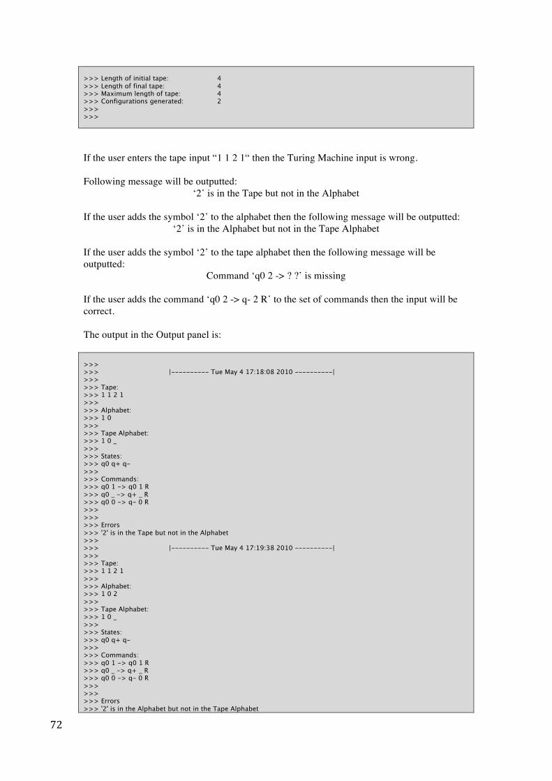
72

>>> Length of initial tape: 4 >>> Length of final tape: 4 >>> Maximum length of tape: 4 >>> Configurations generated: 2 >>> >>>

If the user enters the tape input “1 1 2 1“ then the Turing Machine input is wrong. Following message will be outputted:

‘2’ is in the Tape but not in the Alphabet

If the user adds the symbol ‘2’ to the alphabet then the following message will be outputted: ‘2’ is in the Alphabet but not in the Tape Alphabet

If the user adds the symbol ‘2’ to the tape alphabet then the following message will be outputted:

Command ‘q0 2 -> ? ?’ is missing If the user adds the command ‘q0 2 -> q- 2 R’ to the set of commands then the input will be correct. The output in the Output panel is: >>> >>> |---------- Tue May 4 17:18:08 2010 ----------| >>> >>> Tape: >>> 1 1 2 1 >>> >>> Alphabet: >>> 1 0 >>> >>> Tape Alphabet: >>> 1 0 _ >>> >>> States: >>> q0 q+ q- >>> >>> Commands: >>> q0 1 -> q0 1 R >>> q0 _ -> q+ _ R >>> q0 0 -> q- 0 R >>> >>> >>> Errors >>> '2' is in the Tape but not in the Alphabet >>> >>> |---------- Tue May 4 17:19:38 2010 ----------| >>> >>> Tape: >>> 1 1 2 1 >>> >>> Alphabet: >>> 1 0 2 >>> >>> Tape Alphabet: >>> 1 0 _ >>> >>> States: >>> q0 q+ q- >>> >>> Commands: >>> q0 1 -> q0 1 R >>> q0 _ -> q+ _ R >>> q0 0 -> q- 0 R >>> >>> >>> Errors >>> '2' is in the Alphabet but not in the Tape Alphabet

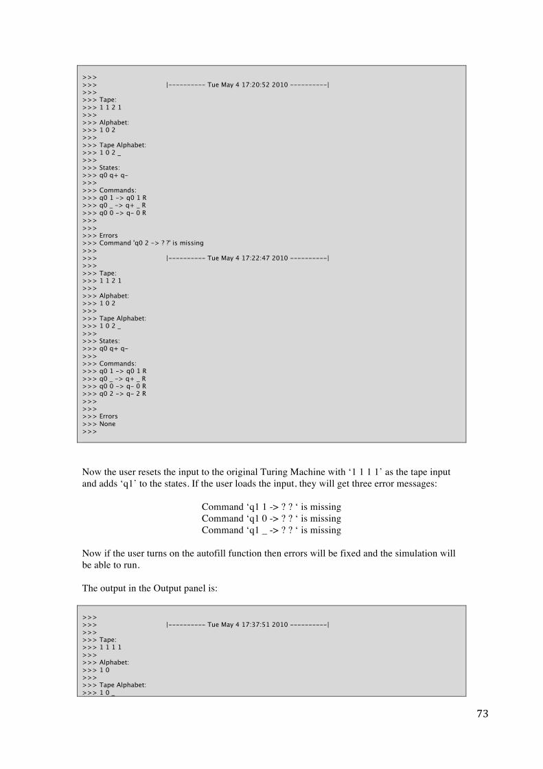
73

>>> >>> |---------- Tue May 4 17:20:52 2010 ----------| >>> >>> Tape: >>> 1 1 2 1 >>> >>> Alphabet: >>> 1 0 2 >>> >>> Tape Alphabet: >>> 1 0 2 _ >>> >>> States: >>> q0 q+ q- >>> >>> Commands: >>> q0 1 -> q0 1 R >>> q0 _ -> q+ _ R >>> q0 0 -> q- 0 R >>> >>> >>> Errors >>> Command 'q0 2 -> ? ?' is missing >>> >>> |---------- Tue May 4 17:22:47 2010 ----------| >>> >>> Tape: >>> 1 1 2 1 >>> >>> Alphabet: >>> 1 0 2 >>> >>> Tape Alphabet: >>> 1 0 2 _ >>> >>> States: >>> q0 q+ q- >>> >>> Commands: >>> q0 1 -> q0 1 R >>> q0 _ -> q+ _ R >>> q0 0 -> q- 0 R >>> q0 2 -> q- 2 R >>> >>> >>> Errors >>> None >>>

Now the user resets the input to the original Turing Machine with ‘1 1 1 1’ as the tape input and adds ‘q1’ to the states. If the user loads the input, they will get three error messages:

Command ‘q1 1 -> ? ? ‘ is missing Command ‘q1 0 -> ? ? ‘ is missing Command ‘q1 _ -> ? ? ‘ is missing

Now if the user turns on the autofill function then errors will be fixed and the simulation will be able to run. The output in the Output panel is: >>> >>> |---------- Tue May 4 17:37:51 2010 ----------| >>> >>> Tape: >>> 1 1 1 1 >>> >>> Alphabet: >>> 1 0 >>> >>> Tape Alphabet: >>> 1 0 _

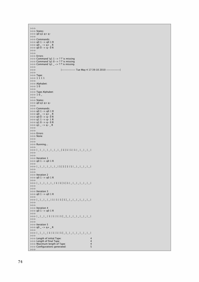
74

>>> >>> States: >>> q0 q1 q+ q- >>> >>> Commands: >>> q0 1 -> q0 1 R >>> q0 _ -> q+ _ R >>> q0 0 -> q- 0 R >>> >>> >>> Errors >>> Command 'q1 1 -> ? ?' is missing >>> Command 'q1 0 -> ? ?' is missing >>> Command 'q1 _ -> ? ?' is missing >>> >>> |---------- Tue May 4 17:39:10 2010 ----------| >>> >>> Tape: >>> 1 1 1 1 >>> >>> Alphabet: >>> 1 0 >>> >>> Tape Alphabet: >>> 1 0 _ >>> >>> States: >>> q0 q1 q+ q- >>> >>> Commands: >>> q0 1 -> q0 1 R >>> q0 _ -> q+ _ R >>> q0 0 -> q- 0 R >>> q1 1 -> q- 1 R >>> q1 0 -> q- 0 R >>> q1 _ -> q- _ R >>> >>> >>> Errors >>> None >>> >>> >>> Running... >>> >>> | _ | _ | _ | _ | _ | _ | _ [ 1 ] 1 | 1 | 1 | _ | _ | _ | _ | >>> >>> >>> Iteration 1 >>> q0 1 -> q0 1 R >>> >>> | _ | _ | _ | _ | _ | _ | 1 [ 1 ] 1 | 1 | _ | _ | _ | _ | _ | >>> >>> >>> Iteration 2 >>> q0 1 -> q0 1 R >>> >>> | _ | _ | _ | _ | _ | 1 | 1 [ 1 ] 1 | _ | _ | _ | _ | _ | _ | >>> >>> >>> Iteration 3 >>> q0 1 -> q0 1 R >>> >>> | _ | _ | _ | _ | 1 | 1 | 1 [ 1 ] _ | _ | _ | _ | _ | _ | _ | >>> >>> >>> Iteration 4 >>> q0 1 -> q0 1 R >>> >>> | _ | _ | _ | 1 | 1 | 1 | 1 [ _ ] _ | _ | _ | _ | _ | _ | _ | >>> >>> >>> Iteration 5 >>> q0 _ -> q+ _ R >>> >>> | _ | _ | _ | 1 | 1 | 1 | 1 [ _ ] _ | _ | _ | _ | _ | _ | _ | >>> >>> Length of initial Tape: 4 >>> Length of final Tape: 4 >>> Maximum length of Tape: 4 >>> Configurations generated: 5 >>>

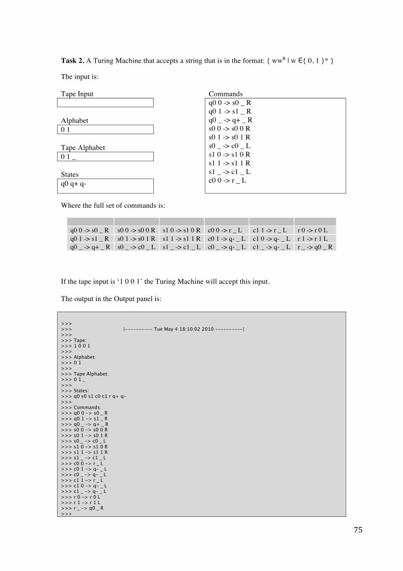
75

Task 2. A Turing Machine that accepts a string that is in the format: { wwR | w ∈{ 0, 1 }* } The input is: Tape Input Commands Alphabet 0 1 Tape Alphabet 0 1 _ States q0 q+ q-

q0 0 -> s0 _ R q0 1 -> s1 _ R q0 _ -> q+ _ R s0 0 -> s0 0 R s0 1 -> s0 1 R s0 _ -> c0 _ L s1 0 -> s1 0 R s1 1 -> s1 1 R s1 _ -> c1 _ L c0 0 -> r _ L

Where the full set of commands is:

q0 0 -> s0 _ R s0 0 -> s0 0 R s1 0 -> s1 0 R c0 0 -> r _ L c1 1 -> r _ L r 0 -> r 0 L q0 1 -> s1 _ R s0 1 -> s0 1 R s1 1 -> s1 1 R c0 1 -> q- _ L c1 0 -> q- _ L r 1 -> r 1 L q0 _ -> q+ _ R s0 _ -> c0 _ L s1 _ -> c1 _ L c0 _ -> q- _ L c1 _ -> q- _ L r _ -> q0 _ R

If the tape input is ‘1 0 0 1’ the Turing Machine will accept this input. The output in the Output panel is: >>> >>> |---------- Tue May 4 18:10:02 2010 ----------| >>> >>> Tape: >>> 1 0 0 1 >>> >>> Alphabet: >>> 0 1 >>> >>> Tape Alphabet: >>> 0 1 _ >>> >>> States: >>> q0 s0 s1 c0 c1 r q+ q- >>> >>> Commands: >>> q0 0 -> s0 _ R >>> q0 1 -> s1 _ R >>> q0 _ -> q+ _ R >>> s0 0 -> s0 0 R >>> s0 1 -> s0 1 R >>> s0 _ -> c0 _ L >>> s1 0 -> s1 0 R >>> s1 1 -> s1 1 R >>> s1 _ -> c1 _ L >>> c0 0 -> r _ L >>> c0 1 -> q- _ L >>> c0 _ -> q- _ L >>> c1 1 -> r _ L >>> c1 0 -> q- _ L >>> c1 _ -> q- _ L >>> r 0 -> r 0 L >>> r 1 -> r 1 L >>> r _ -> q0 _ R >>>

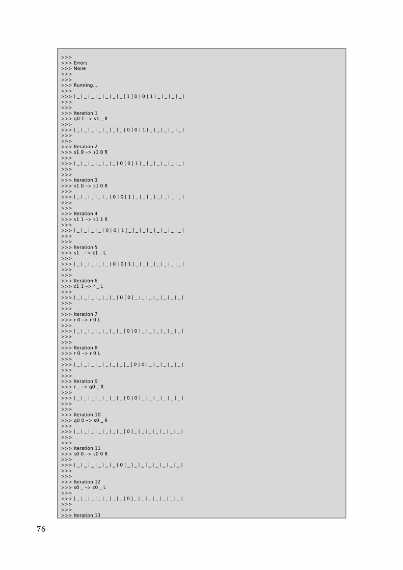
76

>>> >>> Errors >>> None >>> >>> >>> Running... >>> >>> | _ | _ | _ | _ | _ | _ | _ [ 1 ] 0 | 0 | 1 | _ | _ | _ | _ | >>> >>> >>> Iteration 1 >>> q0 1 -> s1 _ R >>> >>> | _ | _ | _ | _ | _ | _ | _ [ 0 ] 0 | 1 | _ | _ | _ | _ | _ | >>> >>> >>> Iteration 2 >>> s1 0 -> s1 0 R >>> >>> | _ | _ | _ | _ | _ | _ | 0 [ 0 ] 1 | _ | _ | _ | _ | _ | _ | >>> >>> >>> Iteration 3 >>> s1 0 -> s1 0 R >>> >>> | _ | _ | _ | _ | _ | 0 | 0 [ 1 ] _ | _ | _ | _ | _ | _ | _ | >>> >>> >>> Iteration 4 >>> s1 1 -> s1 1 R >>> >>> | _ | _ | _ | _ | 0 | 0 | 1 [ _ ] _ | _ | _ | _ | _ | _ | _ | >>> >>> >>> Iteration 5 >>> s1 _ -> c1 _ L >>> >>> | _ | _ | _ | _ | _ | 0 | 0 [ 1 ] _ | _ | _ | _ | _ | _ | _ | >>> >>> >>> Iteration 6 >>> c1 1 -> r _ L >>> >>> | _ | _ | _ | _ | _ | _ | 0 [ 0 ] _ | _ | _ | _ | _ | _ | _ | >>> >>> >>> Iteration 7 >>> r 0 -> r 0 L >>> >>> | _ | _ | _ | _ | _ | _ | _ [ 0 ] 0 | _ | _ | _ | _ | _ | _ | >>> >>> >>> Iteration 8 >>> r 0 -> r 0 L >>> >>> | _ | _ | _ | _ | _ | _ | _ [ _ ] 0 | 0 | _ | _ | _ | _ | _ | >>> >>> >>> Iteration 9 >>> r _ -> q0 _ R >>> >>> | _ | _ | _ | _ | _ | _ | _ [ 0 ] 0 | _ | _ | _ | _ | _ | _ | >>> >>> >>> Iteration 10 >>> q0 0 -> s0 _ R >>> >>> | _ | _ | _ | _ | _ | _ | _ [ 0 ] _ | _ | _ | _ | _ | _ | _ | >>> >>> >>> Iteration 11 >>> s0 0 -> s0 0 R >>> >>> | _ | _ | _ | _ | _ | _ | 0 [ _ ] _ | _ | _ | _ | _ | _ | _ | >>> >>> >>> Iteration 12 >>> s0 _ -> c0 _ L >>> >>> | _ | _ | _ | _ | _ | _ | _ [ 0 ] _ | _ | _ | _ | _ | _ | _ | >>> >>> >>> Iteration 13

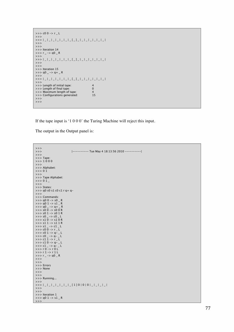
77

>>> c0 0 -> r _ L >>> >>> | _ | _ | _ | _ | _ | _ | _ [ _ ] _ | _ | _ | _ | _ | _ | _ | >>> >>> >>> Iteration 14 >>> r _ -> q0 _ R >>> >>> | _ | _ | _ | _ | _ | _ | _ [ _ ] _ | _ | _ | _ | _ | _ | _ | >>> >>> >>> Iteration 15 >>> q0 _ -> q+ _ R >>> >>> | _ | _ | _ | _ | _ | _ | _ [ _ ] _ | _ | _ | _ | _ | _ | _ | >>> >>> Length of initial tape: 4 >>> Length of final tape: 0 >>> Maximum length of tape: 4 >>> Configurations generated: 15 >>> >>> If the tape input is ‘1 0 0 0’ the Turing Machine will reject this input. The output in the Output panel is: >>> >>> |---------- Tue May 4 18:13:56 2010 ----------| >>> >>> Tape: >>> 1 0 0 0 >>> >>> Alphabet: >>> 0 1 >>> >>> Tape Alphabet: >>> 0 1 _ >>> >>> States: >>> q0 s0 s1 c0 c1 r q+ q- >>> >>> Commands: >>> q0 0 -> s0 _ R >>> q0 1 -> s1 _ R >>> q0 _ -> q+ _ R >>> s0 0 -> s0 0 R >>> s0 1 -> s0 1 R >>> s0 _ -> c0 _ L >>> s1 0 -> s1 0 R >>> s1 1 -> s1 1 R >>> s1 _ -> c1 _ L >>> c0 0 -> r _ L >>> c0 1 -> q- _ L >>> c0 _ -> q- _ L >>> c1 1 -> r _ L >>> c1 0 -> q- _ L >>> c1 _ -> q- _ L >>> r 0 -> r 0 L >>> r 1 -> r 1 L >>> r _ -> q0 _ R >>> >>> >>> Errors >>> None >>> >>> >>> Running... >>> >>> | _ | _ | _ | _ | _ | _ | _ [ 1 ] 0 | 0 | 0 | _ | _ | _ | _ | >>> >>> >>> Iteration 1 >>> q0 1 -> s1 _ R >>>

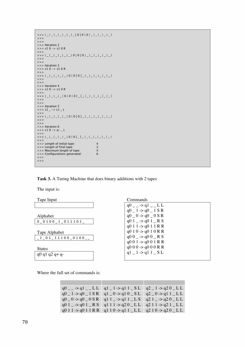
78

>>> | _ | _ | _ | _ | _ | _ | _ [ 0 ] 0 | 0 | _ | _ | _ | _ | _ | >>> >>> >>> Iteration 2 >>> s1 0 -> s1 0 R >>> >>> | _ | _ | _ | _ | _ | _ | 0 [ 0 ] 0 | _ | _ | _ | _ | _ | _ | >>> >>> >>> Iteration 3 >>> s1 0 -> s1 0 R >>> >>> | _ | _ | _ | _ | _ | 0 | 0 [ 0 ] _ | _ | _ | _ | _ | _ | _ | >>> >>> >>> Iteration 4 >>> s1 0 -> s1 0 R >>> >>> | _ | _ | _ | _ | 0 | 0 | 0 [ _ ] _ | _ | _ | _ | _ | _ | _ | >>> >>> >>> Iteration 5 >>> s1 _ -> c1 _ L >>> >>> | _ | _ | _ | _ | _ | 0 | 0 [ 0 ] _ | _ | _ | _ | _ | _ | _ | >>> >>> >>> Iteration 6 >>> c1 0 -> q- _ L >>> >>> | _ | _ | _ | _ | _ | 0 | 0 [ _ ] _ | _ | _ | _ | _ | _ | _ | >>> >>> Length of initial tape: 4 >>> Length of final tape: 2 >>> Maximum length of tape: 4 >>> Configurations generated: 6 >>> >>> Task 3. A Turing Machine that does binary additions with 2 tapes The input is: Tape Input Commands Alphabet 0 _ 0 1 0 0 _ 1 _ 0 1 1 1 0 1 _ Tape Alphabet _ 1 _ 0 1 _ 1 1 1 0 0 _ 0 1 0 0 _ _ States q0 q1 q2 q+ q-

q0 _ _ -> q1 _ _ L L q0 _ 1 -> q0 _ 1 S R q0 _ 0 -> q0 _ 0 S R q0 1 _ -> q0 1 _ R S q0 1 1 -> q0 1 1 R R q0 1 0 -> q0 1 0 R R q0 0 _ -> q0 0 _ R S q0 0 1 -> q0 0 1 R R q0 0 0 -> q0 0 0 R R q1 _ 1 -> q1 1 _ S L


q0 _ _ -> q1 _ _ L L q1 _ 1 -> q1 1 _ S L q2 _ 1 -> q2 0 _ L L q0 _ 1 -> q0 _ 1 S R q1 _ 0 -> q1 0 _ S L q2 _ 0 -> q1 1 _ L L q0 _ 0 -> q0 _ 0 S R q1 1 _ -> q1 1 _ L S q2 1 _ -> q2 0 _ L L q0 1 _ -> q0 1 _ R S q1 1 1 -> q2 0 _ L L q2 1 1 -> q2 1 _ L L q0 1 1 -> q0 1 1 R R q1 1 0 -> q1 1 _ L L q2 1 0 -> q2 0 _ L L

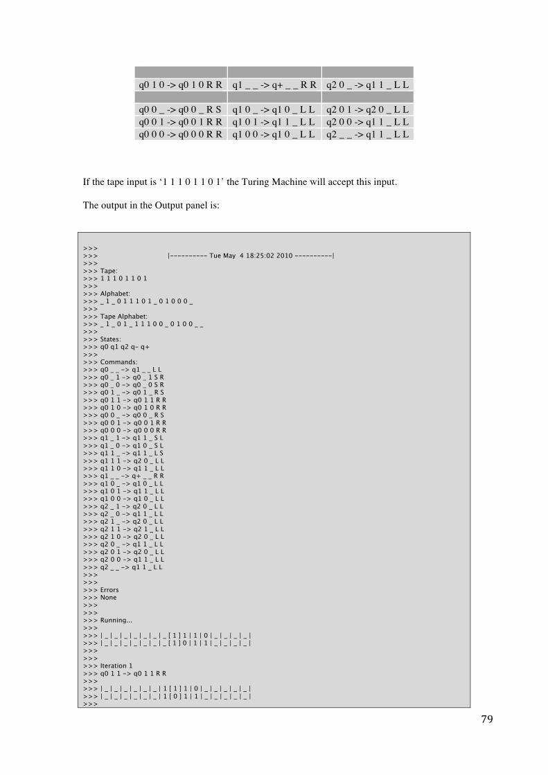
79

q0 1 0 -> q0 1 0 R R q1 _ _ -> q+ _ _ R R q2 0 _ -> q1 1 _ L L q0 0 _ -> q0 0 _ R S q1 0 _ -> q1 0 _ L L q2 0 1 -> q2 0 _ L L q0 0 1 -> q0 0 1 R R q1 0 1 -> q1 1 _ L L q2 0 0 -> q1 1 _ L L q0 0 0 -> q0 0 0 R R q1 0 0 -> q1 0 _ L L q2 _ _ -> q1 1 _ L L

If the tape input is ‘1 1 1 0 1 1 0 1’ the Turing Machine will accept this input. The output in the Output panel is:

>>> >>> |---------- Tue May 4 18:25:02 2010 ----------| >>> >>> Tape: >>> 1 1 1 0 1 1 0 1 >>> >>> Alphabet: >>> _ 1 _ 0 1 1 1 0 1 _ 0 1 0 0 0 _ >>> >>> Tape Alphabet: >>> _ 1 _ 0 1 _ 1 1 1 0 0 _ 0 1 0 0 _ _ >>> >>> States: >>> q0 q1 q2 q- q+ >>> >>> Commands: >>> q0 _ _ -> q1 _ _ L L >>> q0 _ 1 -> q0 _ 1 S R >>> q0 _ 0 -> q0 _ 0 S R >>> q0 1 _ -> q0 1 _ R S >>> q0 1 1 -> q0 1 1 R R >>> q0 1 0 -> q0 1 0 R R >>> q0 0 _ -> q0 0 _ R S >>> q0 0 1 -> q0 0 1 R R >>> q0 0 0 -> q0 0 0 R R >>> q1 _ 1 -> q1 1 _ S L >>> q1 _ 0 -> q1 0 _ S L >>> q1 1 _ -> q1 1 _ L S >>> q1 1 1 -> q2 0 _ L L >>> q1 1 0 -> q1 1 _ L L >>> q1 _ _ -> q+ _ _ R R >>> q1 0 _ -> q1 0 _ L L >>> q1 0 1 -> q1 1 _ L L >>> q1 0 0 -> q1 0 _ L L >>> q2 _ 1 -> q2 0 _ L L >>> q2 _ 0 -> q1 1 _ L L >>> q2 1 _ -> q2 0 _ L L >>> q2 1 1 -> q2 1 _ L L >>> q2 1 0 -> q2 0 _ L L >>> q2 0 _ -> q1 1 _ L L >>> q2 0 1 -> q2 0 _ L L >>> q2 0 0 -> q1 1 _ L L >>> q2 _ _ -> q1 1 _ L L >>> >>> >>> Errors >>> None >>> >>> >>> Running... >>> >>> | _ | _ | _ | _ | _ | _ | _ [ 1 ] 1 | 1 | 0 | _ | _ | _ | _ | >>> | _ | _ | _ | _ | _ | _ | _ [ 1 ] 0 | 1 | 1 | _ | _ | _ | _ | >>> >>> >>> Iteration 1 >>> q0 1 1 -> q0 1 1 R R >>> >>> | _ | _ | _ | _ | _ | _ | 1 [ 1 ] 1 | 0 | _ | _ | _ | _ | _ | >>> | _ | _ | _ | _ | _ | _ | 1 [ 0 ] 1 | 1 | _ | _ | _ | _ | _ | >>>

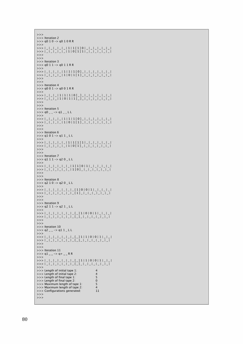
80

>>> >>> Iteration 2 >>> q0 1 0 -> q0 1 0 R R >>> >>> | _ | _ | _ | _ | _ | 1 | 1 [ 1 ] 0 | _ | _ | _ | _ | _ | _ | >>> | _ | _ | _ | _ | _ | 1 | 0 [ 1 ] 1 | _ | _ | _ | _ | _ | _ | >>> >>> >>> Iteration 3 >>> q0 1 1 -> q0 1 1 R R >>> >>> | _ | _ | _ | _ | 1 | 1 | 1 [ 0 ] _ | _ | _ | _ | _ | _ | _ | >>> | _ | _ | _ | _ | 1 | 0 | 1 [ 1 ] _ | _ | _ | _ | _ | _ | _ | >>> >>> >>> Iteration 4 >>> q0 0 1 -> q0 0 1 R R >>> >>> | _ | _ | _ | 1 | 1 | 1 | 0 [ _ ] _ | _ | _ | _ | _ | _ | _ | >>> | _ | _ | _ | 1 | 0 | 1 | 1 [ _ ] _ | _ | _ | _ | _ | _ | _ | >>> >>> >>> Iteration 5 >>> q0 _ _ -> q1 _ _ L L >>> >>> | _ | _ | _ | _ | 1 | 1 | 1 [ 0 ] _ | _ | _ | _ | _ | _ | _ | >>> | _ | _ | _ | _ | 1 | 0 | 1 [ 1 ] _ | _ | _ | _ | _ | _ | _ | >>> >>> >>> Iteration 6 >>> q1 0 1 -> q1 1 _ L L >>> >>> | _ | _ | _ | _ | _ | 1 | 1 [ 1 ] 1 | _ | _ | _ | _ | _ | _ | >>> | _ | _ | _ | _ | _ | 1 | 0 [ 1 ] _ | _ | _ | _ | _ | _ | _ | >>> >>> >>> Iteration 7 >>> q1 1 1 -> q2 0 _ L L >>> >>> | _ | _ | _ | _ | _ | _ | 1 [ 1 ] 0 | 1 | _ | _ | _ | _ | _ | >>> | _ | _ | _ | _ | _ | _ | 1 [ 0 ] _ | _ | _ | _ | _ | _ | _ | >>> >>> >>> Iteration 8 >>> q2 1 0 -> q2 0 _ L L >>> >>> | _ | _ | _ | _ | _ | _ | _ [ 1 ] 0 | 0 | 1 | _ | _ | _ | _ | >>> | _ | _ | _ | _ | _ | _ | _ [ 1 ] _ | _ | _ | _ | _ | _ | _ | >>> >>> >>> Iteration 9 >>> q2 1 1 -> q2 1 _ L L >>> >>> | _ | _ | _ | _ | _ | _ | _ [ _ ] 1 | 0 | 0 | 1 | _ | _ | _ | >>> | _ | _ | _ | _ | _ | _ | _ [ _ ] _ | _ | _ | _ | _ | _ | _ | >>> >>> >>> Iteration 10 >>> q2 _ _ -> q1 1 _ L L >>> >>> | _ | _ | _ | _ | _ | _ | _ [ _ ] 1 | 1 | 0 | 0 | 1 | _ | _ | >>> | _ | _ | _ | _ | _ | _ | _ [ _ ] _ | _ | _ | _ | _ | _ | _ | >>> >>> >>> Iteration 11 >>> q1 _ _ -> q+ _ _ R R >>> >>> | _ | _ | _ | _ | _ | _ | _ [ _ ] 1 | 1 | 0 | 0 | 1 | _ | _ | >>> | _ | _ | _ | _ | _ | _ | _ [ _ ] _ | _ | _ | _ | _ | _ | _ | >>> >>> Length of initial tape 1: 4 >>> Length of initial tape 2: 4 >>> Length of final tape 1: 5 >>> Length of final tape 2: 0 >>> Maximum length of tape 1: 5 >>> Maximum length of tape 2: 4 >>> Configurations generated: 11 >>> >>>

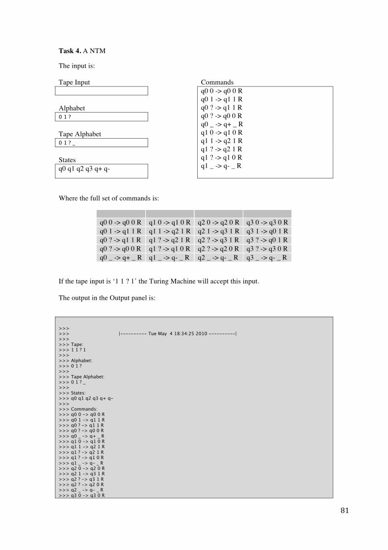
81

Task 4. A NTM

The input is: Tape Input Commands Alphabet 0 1 ? Tape Alphabet 0 1 ? _ States q0 q1 q2 q3 q+ q-

q0 0 -> q0 0 R q0 1 -> q1 1 R q0 ? -> q1 1 R q0 ? -> q0 0 R q0 _ -> q+ _ R q1 0 -> q1 0 R q1 1 -> q2 1 R q1 ? -> q2 1 R q1 ? -> q1 0 R q1 _ -> q- _ R


q0 0 -> q0 0 R q1 0 -> q1 0 R q2 0 -> q2 0 R q3 0 -> q3 0 R q0 1 -> q1 1 R q1 1 -> q2 1 R q2 1 -> q3 1 R q3 1 -> q0 1 R q0 ? -> q1 1 R q1 ? -> q2 1 R q2 ? -> q3 1 R q3 ? -> q0 1 R q0 ? -> q0 0 R q1 ? -> q1 0 R q2 ? -> q2 0 R q3 ? -> q3 0 R q0 _ -> q+ _ R q1 _ -> q- _ R q2 _ -> q- _ R q3 _ -> q- _ R

If the tape input is ‘1 1 ? 1’ the Turing Machine will accept this input. The output in the Output panel is:

>>> >>> |---------- Tue May 4 18:34:25 2010 ----------| >>> >>> Tape: >>> 1 1 ? 1 >>> >>> Alphabet: >>> 0 1 ? >>> >>> Tape Alphabet: >>> 0 1 ? _ >>> >>> States: >>> q0 q1 q2 q3 q+ q- >>> >>> Commands: >>> q0 0 -> q0 0 R >>> q0 1 -> q1 1 R >>> q0 ? -> q1 1 R >>> q0 ? -> q0 0 R >>> q0 _ -> q+ _ R >>> q1 0 -> q1 0 R >>> q1 1 -> q2 1 R >>> q1 ? -> q2 1 R >>> q1 ? -> q1 0 R >>> q1 _ -> q- _ R >>> q2 0 -> q2 0 R >>> q2 1 -> q3 1 R >>> q2 ? -> q3 1 R >>> q2 ? -> q2 0 R >>> q2 _ -> q- _ R >>> q3 0 -> q3 0 R

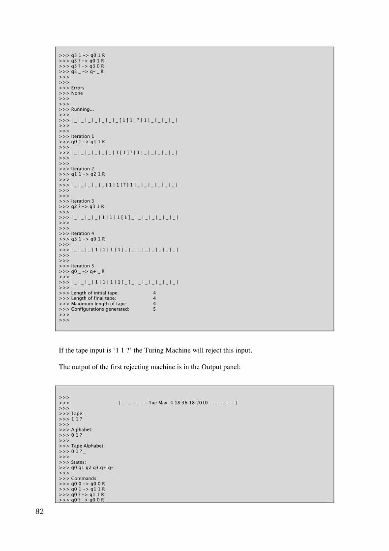
82

>>> q3 1 -> q0 1 R >>> q3 ? -> q0 1 R >>> q3 ? -> q3 0 R >>> q3 _ -> q- _ R >>> >>> >>> Errors >>> None >>> >>> >>> Running... >>> >>> | _ | _ | _ | _ | _ | _ | _ [ 1 ] 1 | ? | 1 | _ | _ | _ | _ | >>> >>> >>> Iteration 1 >>> q0 1 -> q1 1 R >>> >>> | _ | _ | _ | _ | _ | _ | 1 [ 1 ] ? | 1 | _ | _ | _ | _ | _ | >>> >>> >>> Iteration 2 >>> q1 1 -> q2 1 R >>> >>> | _ | _ | _ | _ | _ | 1 | 1 [ ? ] 1 | _ | _ | _ | _ | _ | _ | >>> >>> >>> Iteration 3 >>> q2 ? -> q3 1 R >>> >>> | _ | _ | _ | _ | 1 | 1 | 1 [ 1 ] _ | _ | _ | _ | _ | _ | _ | >>> >>> >>> Iteration 4 >>> q3 1 -> q0 1 R >>> >>> | _ | _ | _ | 1 | 1 | 1 | 1 [ _ ] _ | _ | _ | _ | _ | _ | _ | >>> >>> >>> Iteration 5 >>> q0 _ -> q+ _ R >>> >>> | _ | _ | _ | 1 | 1 | 1 | 1 [ _ ] _ | _ | _ | _ | _ | _ | _ | >>> >>> Length of initial tape: 4 >>> Length of final tape: 4 >>> Maximum length of tape: 4 >>> Configurations generated: 5 >>> >>>

If the tape input is ‘1 1 ?’ the Turing Machine will reject this input. The output of the first rejecting machine is in the Output panel:

>>> >>> |---------- Tue May 4 18:36:18 2010 ----------| >>> >>> Tape: >>> 1 1 ? >>> >>> Alphabet: >>> 0 1 ? >>> >>> Tape Alphabet: >>> 0 1 ? _ >>> >>> States: >>> q0 q1 q2 q3 q+ q- >>> >>> Commands: >>> q0 0 -> q0 0 R >>> q0 1 -> q1 1 R >>> q0 ? -> q1 1 R >>> q0 ? -> q0 0 R

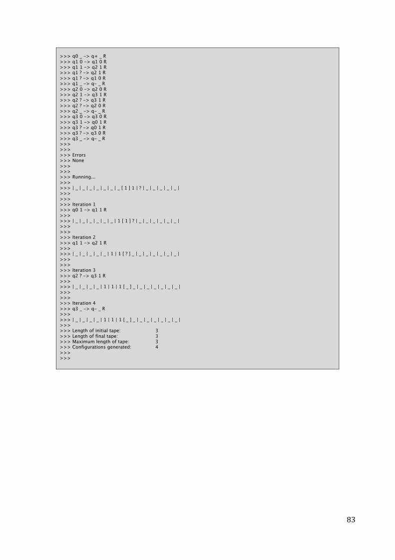
83

>>> q0 _ -> q+ _ R >>> q1 0 -> q1 0 R >>> q1 1 -> q2 1 R >>> q1 ? -> q2 1 R >>> q1 ? -> q1 0 R >>> q1 _ -> q- _ R >>> q2 0 -> q2 0 R >>> q2 1 -> q3 1 R >>> q2 ? -> q3 1 R >>> q2 ? -> q2 0 R >>> q2 _ -> q- _ R >>> q3 0 -> q3 0 R >>> q3 1 -> q0 1 R >>> q3 ? -> q0 1 R >>> q3 ? -> q3 0 R >>> q3 _ -> q- _ R >>> >>> >>> Errors >>> None >>> >>> >>> Running... >>> >>> | _ | _ | _ | _ | _ | _ | _ [ 1 ] 1 | ? | _ | _ | _ | _ | _ | >>> >>> >>> Iteration 1 >>> q0 1 -> q1 1 R >>> >>> | _ | _ | _ | _ | _ | _ | 1 [ 1 ] ? | _ | _ | _ | _ | _ | _ | >>> >>> >>> Iteration 2 >>> q1 1 -> q2 1 R >>> >>> | _ | _ | _ | _ | _ | 1 | 1 [ ? ] _ | _ | _ | _ | _ | _ | _ | >>> >>> >>> Iteration 3 >>> q2 ? -> q3 1 R >>> >>> | _ | _ | _ | _ | 1 | 1 | 1 [ _ ] _ | _ | _ | _ | _ | _ | _ | >>> >>> >>> Iteration 4 >>> q3 _ -> q- _ R >>> >>> | _ | _ | _ | _ | 1 | 1 | 1 [ _ ] _ | _ | _ | _ | _ | _ | _ | >>> >>> Length of initial tape: 3 >>> Length of final tape: 3 >>> Maximum length of tape: 3 >>> Configurations generated: 4 >>> >>>

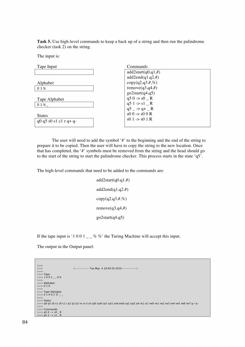
84

Task 5. Use high-level commands to keep a back up of a string and then run the palindrome checker (task 2) on the string.

The input is: Tape Input Commands Alphabet 0 1 % Tape Alphabet 0 1 % _ States q0 q5 s0 s1 c1 r q+ q-

add2start(q0,q1,#) add2end(q1,q2,#) copy(q2,q3,#,%) remove(q3,q4,#) go2start(q4,q5) q5 0 -> s0 _ R q5 1 -> s1 _ R q5 _ -> q+ _ R s0 0 -> s0 0 R s0 1 -> s0 1 R

The user will need to add the symbol ‘#’ to the beginning and the end of the string to prepare it to be copied. Then the user will have to copy the string to the new location. Once that has completed, the ‘#’ symbols must be removed from the string and the head should go to the start of the string to start the palindrome checker. This process starts in the state ‘q5’.

The high-level commands that need to be added to the commands are:

add2start(q0,q1,#)

add2end(q1,q2,#)

copy(q2,q3,#,%)

remove(q3,q4,#)

go2start(q4,q5)

If the tape input is ‘1 0 0 1 _ _ % %’ the Turing Machine will accept this input. The output in the Output panel:

>>> >>> |---------- Tue May 4 18:49:59 2010 ----------| >>> >>> Tape: >>> 1 0 0 1 _ _ % % >>> >>> Alphabet: >>> 0 1 % >>> >>> Tape Alphabet: >>> 0 1 # % 1' 0' _' _ >>> >>> States: >>> q0 q5 s0 s1 c0 c1 r q1 q2 q3 re st cl cli cp0 cpi0 cp1 cpi1 end endi cp2 cpi2 q4 re1 st1 rw0 rw1 rw2 rw3 rw4 rw5 rw6 rw7 q+ q- >>> >>> Commands: >>> q5 0 -> s0 _ R >>> q5 1 -> s1 _ R

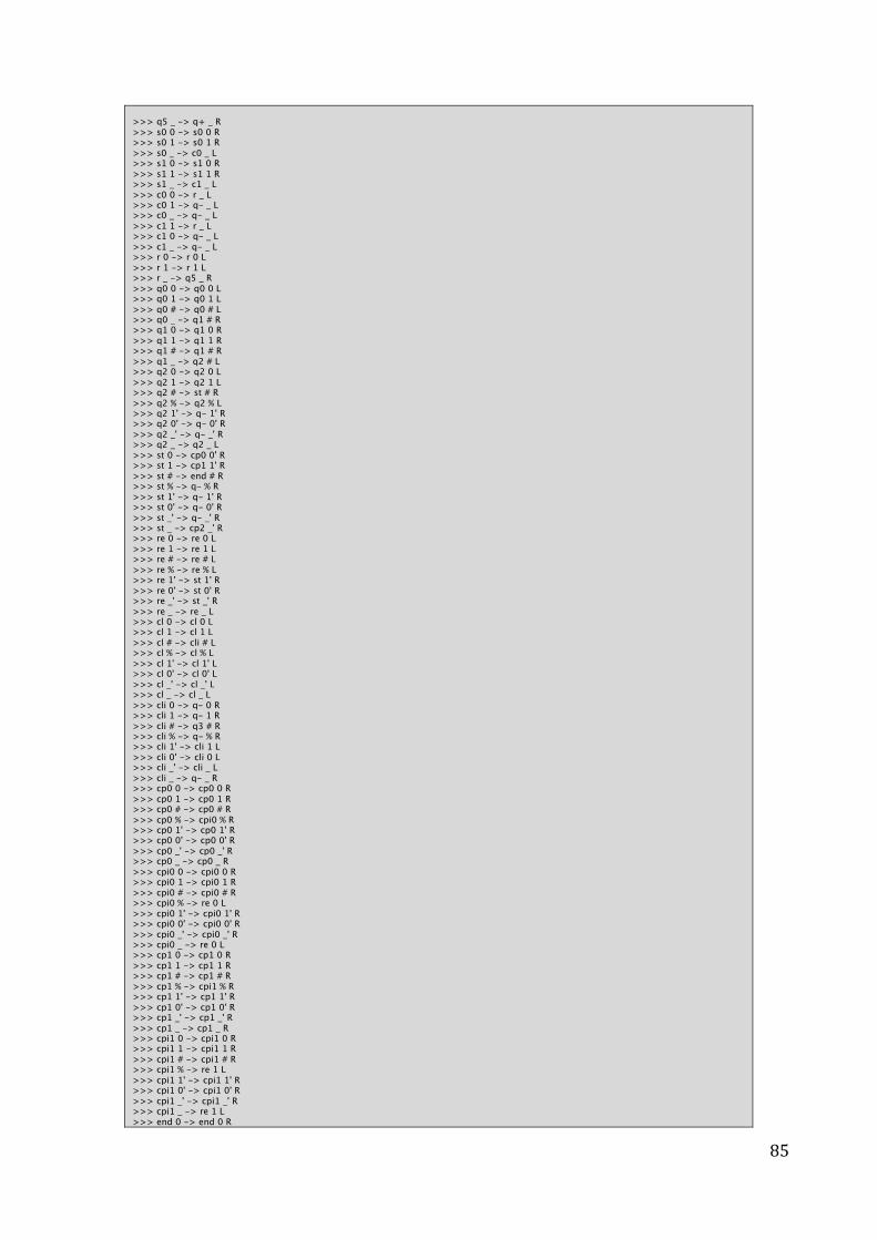
85

>>> q5 _ -> q+ _ R >>> s0 0 -> s0 0 R >>> s0 1 -> s0 1 R >>> s0 _ -> c0 _ L >>> s1 0 -> s1 0 R >>> s1 1 -> s1 1 R >>> s1 _ -> c1 _ L >>> c0 0 -> r _ L >>> c0 1 -> q- _ L >>> c0 _ -> q- _ L >>> c1 1 -> r _ L >>> c1 0 -> q- _ L >>> c1 _ -> q- _ L >>> r 0 -> r 0 L >>> r 1 -> r 1 L >>> r _ -> q5 _ R >>> q0 0 -> q0 0 L >>> q0 1 -> q0 1 L >>> q0 # -> q0 # L >>> q0 _ -> q1 # R >>> q1 0 -> q1 0 R >>> q1 1 -> q1 1 R >>> q1 # -> q1 # R >>> q1 _ -> q2 # L >>> q2 0 -> q2 0 L >>> q2 1 -> q2 1 L >>> q2 # -> st # R >>> q2 % -> q2 % L >>> q2 1' -> q- 1' R >>> q2 0' -> q- 0' R >>> q2 _' -> q- _' R >>> q2 _ -> q2 _ L >>> st 0 -> cp0 0' R >>> st 1 -> cp1 1' R >>> st # -> end # R >>> st % -> q- % R >>> st 1' -> q- 1' R >>> st 0' -> q- 0' R >>> st _' -> q- _' R >>> st _ -> cp2 _' R >>> re 0 -> re 0 L >>> re 1 -> re 1 L >>> re # -> re # L >>> re % -> re % L >>> re 1' -> st 1' R >>> re 0' -> st 0' R >>> re _' -> st _' R >>> re _ -> re _ L >>> cl 0 -> cl 0 L >>> cl 1 -> cl 1 L >>> cl # -> cli # L >>> cl % -> cl % L >>> cl 1' -> cl 1' L >>> cl 0' -> cl 0' L >>> cl _' -> cl _' L >>> cl _ -> cl _ L >>> cli 0 -> q- 0 R >>> cli 1 -> q- 1 R >>> cli # -> q3 # R >>> cli % -> q- % R >>> cli 1' -> cli 1 L >>> cli 0' -> cli 0 L >>> cli _' -> cli _ L >>> cli _ -> q- _ R >>> cp0 0 -> cp0 0 R >>> cp0 1 -> cp0 1 R >>> cp0 # -> cp0 # R >>> cp0 % -> cpi0 % R >>> cp0 1' -> cp0 1' R >>> cp0 0' -> cp0 0' R >>> cp0 _' -> cp0 _' R >>> cp0 _ -> cp0 _ R >>> cpi0 0 -> cpi0 0 R >>> cpi0 1 -> cpi0 1 R >>> cpi0 # -> cpi0 # R >>> cpi0 % -> re 0 L >>> cpi0 1' -> cpi0 1' R >>> cpi0 0' -> cpi0 0' R >>> cpi0 _' -> cpi0 _' R >>> cpi0 _ -> re 0 L >>> cp1 0 -> cp1 0 R >>> cp1 1 -> cp1 1 R >>> cp1 # -> cp1 # R >>> cp1 % -> cpi1 % R >>> cp1 1' -> cp1 1' R >>> cp1 0' -> cp1 0' R >>> cp1 _' -> cp1 _' R >>> cp1 _ -> cp1 _ R >>> cpi1 0 -> cpi1 0 R >>> cpi1 1 -> cpi1 1 R >>> cpi1 # -> cpi1 # R >>> cpi1 % -> re 1 L >>> cpi1 1' -> cpi1 1' R >>> cpi1 0' -> cpi1 0' R >>> cpi1 _' -> cpi1 _' R >>> cpi1 _ -> re 1 L >>> end 0 -> end 0 R

86

>>> end 1 -> end 1 R >>> end # -> q- # R >>> end % -> endi % R >>> end 1' -> q- 1' R >>> end 0' -> q- 0' R >>> end _' -> q- _' R >>> end _ -> end _ R >>> endi 0 -> endi 0 R >>> endi 1 -> endi 1 R >>> endi # -> q- # R >>> endi % -> cl % L >>> endi 1' -> q- 1' R >>> endi 0' -> q- 0' R >>> endi _' -> q- _' R >>> endi _ -> cl % L >>> cp2 0 -> cp2 0 R >>> cp2 1 -> cp2 1 R >>> cp2 # -> cp2 # R >>> cp2 % -> cpi2 % R >>> cp2 1' -> cp2 1' R >>> cp2 0' -> cp2 0' R >>> cp2 _' -> cp2 _' R >>> cp2 _ -> cp2 _ R >>> cpi2 0 -> cpi2 0 R >>> cpi2 1 -> cpi2 1 R >>> cpi2 # -> cpi2 # R >>> cpi2 % -> re _ L >>> cpi2 1' -> cpi2 1' R >>> cpi2 0' -> cpi2 0' R >>> cpi2 _' -> cpi2 _' R >>> cpi2 _ -> re _ L >>> q3 0 -> q3 0 L >>> q3 1 -> q3 1 L >>> q3 # -> q3 # L >>> q3 % -> q3 % L >>> q3 1' -> q3 1' L >>> q3 0' -> q3 0' L >>> q3 _' -> q3 _' L >>> q3 _ -> st1 _ R >>> st1 0 -> st1 0 R >>> st1 1 -> st1 1 R >>> st1 # -> re1 # L >>> st1 % -> st1 % R >>> st1 1' -> st1 1' R >>> st1 0' -> st1 0' R >>> st1 _' -> st1 _' R >>> st1 _ -> q4 _ L >>> re1 0 -> re1 0 L >>> re1 1 -> re1 1 L >>> re1 # -> q- # R >>> re1 % -> re1 % L >>> re1 1' -> re1 1' L >>> re1 0' -> re1 0' L >>> re1 _' -> re1 _' L >>> re1 _ -> rw7 _ R >>> rw0 0 -> rw0 0 R >>> rw0 1 -> rw1 0 R >>> rw0 # -> st1 0 R >>> rw0 % -> rw3 0 R >>> rw0 1' -> rw4 0 R >>> rw0 0' -> rw5 0 R >>> rw0 _' -> rw6 0 R >>> rw0 _ -> q- _ L >>> rw1 0 -> rw0 1 R >>> rw1 1 -> rw1 1 R >>> rw1 # -> st1 1 R >>> rw1 % -> rw3 1 R >>> rw1 1' -> rw4 1 R >>> rw1 0' -> rw5 1 R >>> rw1 _' -> rw6 1 R >>> rw1 _ -> q- _ L >>> rw2 0 -> rw0 # R >>> rw2 1 -> rw1 # R >>> rw2 # -> st1 # R >>> rw2 % -> rw3 # R >>> rw2 1' -> rw4 # R >>> rw2 0' -> rw5 # R >>> rw2 _' -> rw6 # R >>> rw2 _ -> q- _ L >>> rw3 0 -> rw0 % R >>> rw3 1 -> rw1 % R >>> rw3 # -> st1 % R >>> rw3 % -> rw3 % R >>> rw3 1' -> rw4 % R >>> rw3 0' -> rw5 % R >>> rw3 _' -> rw6 % R >>> rw3 _ -> q- _ L >>> rw4 0 -> rw0 1' R >>> rw4 1 -> rw1 1' R >>> rw4 # -> st1 1' R >>> rw4 % -> rw3 1' R >>> rw4 1' -> rw4 1' R >>> rw4 0' -> rw5 1' R >>> rw4 _' -> rw6 1' R >>> rw4 _ -> q- _ L >>> rw5 0 -> rw0 0' R >>> rw5 1 -> rw1 0' R

87

>>> rw5 # -> st1 0' R >>> rw5 % -> rw3 0' R >>> rw5 1' -> rw4 0' R >>> rw5 0' -> rw5 0' R >>> rw5 _' -> rw6 0' R >>> rw5 _ -> q- _ L >>> rw6 0 -> rw0 _' R >>> rw6 1 -> rw1 _' R >>> rw6 # -> st1 _' R >>> rw6 % -> rw3 _' R >>> rw6 1' -> rw4 _' R >>> rw6 0' -> rw5 _' R >>> rw6 _' -> rw6 _' R >>> rw6 _ -> q- _ L >>> rw7 0 -> rw0 _ R >>> rw7 1 -> rw1 _ R >>> rw7 # -> st1 _ R >>> rw7 % -> rw3 _ R >>> rw7 1' -> rw4 _ R >>> rw7 0' -> rw5 _ R >>> rw7 _' -> rw6 _ R >>> rw7 _ -> q- _ L >>> q4 0 -> q4 0 L >>> q4 1 -> q4 1 L >>> q4 # -> q4 # L >>> q4 % -> q4 % L >>> q4 1' -> q4 1' L >>> q4 0' -> q4 0' L >>> q4 _' -> q4 _' L >>> q4 _ -> q5 _ R >>> q0 % -> q- % R >>> q0 1' -> q- 1' R >>> q0 0' -> q- 0' R >>> q0 _' -> q- _' R >>> q5 # -> q- # R >>> q5 % -> q- % R >>> q5 1' -> q- 1' R >>> q5 0' -> q- 0' R >>> q5 _' -> q- _' R >>> s0 # -> q- # R >>> s0 % -> q- % R >>> s0 1' -> q- 1' R >>> s0 0' -> q- 0' R >>> s0 _' -> q- _' R >>> s1 # -> q- # R >>> s1 % -> q- % R >>> s1 1' -> q- 1' R >>> s1 0' -> q- 0' R >>> s1 _' -> q- _' R >>> c0 # -> q- # R >>> c0 % -> q- % R >>> c0 1' -> q- 1' R >>> c0 0' -> q- 0' R >>> c0 _' -> q- _' R >>> c1 # -> q- # R >>> c1 % -> q- % R >>> c1 1' -> q- 1' R >>> c1 0' -> q- 0' R >>> c1 _' -> q- _' R >>> r # -> q- # R >>> r % -> q- % R >>> r 1' -> q- 1' R >>> r 0' -> q- 0' R >>> r _' -> q- _' R >>> q1 % -> q- % R >>> q1 1' -> q- 1' R >>> q1 0' -> q- 0' R >>> q1 _' -> q- _' R >>> >>> >>> Errors >>> None >>> >>> >>> Running... >>> >>> | _ | _ | _ | _ | _ | _ | _ [ 1 ] 0 | 0 | 1 | _ | _ | % | % | >>> >>> >>> Iteration 1 >>> q0 1 -> q0 1 L >>> >>> | _ | _ | _ | _ | _ | _ | _ [ _ ] 1 | 0 | 0 | 1 | _ | _ | % | >>> >>> >>> Iteration 2 >>> q0 _ -> q1 # R >>> >>> | _ | _ | _ | _ | _ | _ | # [ 1 ] 0 | 0 | 1 | _ | _ | % | % | >>> >>> >>> Iteration 3 >>> q1 1 -> q1 1 R >>> >>> | _ | _ | _ | _ | _ | # | 1 [ 0 ] 0 | 1 | _ | _ | % | % | _ | >>> >>>

88

>>> Iteration 4 >>> q1 0 -> q1 0 R >>> >>> | _ | _ | _ | _ | # | 1 | 0 [ 0 ] 1 | _ | _ | % | % | _ | _ | >>> >>> >>> Iteration 5 >>> q1 0 -> q1 0 R >>> >>> | _ | _ | _ | # | 1 | 0 | 0 [ 1 ] _ | _ | % | % | _ | _ | _ | >>> >>> >>> Iteration 6 >>> q1 1 -> q1 1 R >>> >>> | _ | _ | # | 1 | 0 | 0 | 1 [ _ ] _ | % | % | _ | _ | _ | _ | >>> >>> >>> Iteration 7 >>> q1 _ -> q2 # L >>> >>> | _ | _ | _ | # | 1 | 0 | 0 [ 1 ] # | _ | % | % | _ | _ | _ | >>> >>> >>> Iteration 8 >>> q2 1 -> q2 1 L >>> >>> | _ | _ | _ | _ | # | 1 | 0 [ 0 ] 1 | # | _ | % | % | _ | _ | >>> >>> >>> Iteration 9 >>> q2 0 -> q2 0 L >>> >>> | _ | _ | _ | _ | _ | # | 1 [ 0 ] 0 | 1 | # | _ | % | % | _ | >>> >>> >>> Iteration 10 >>> q2 0 -> q2 0 L >>> >>> | _ | _ | _ | _ | _ | _ | # [ 1 ] 0 | 0 | 1 | # | _ | % | % | >>> >>> >>> Iteration 11 >>> q2 1 -> q2 1 L >>> >>> | _ | _ | _ | _ | _ | _ | _ [ # ] 1 | 0 | 0 | 1 | # | _ | % | >>> >>> >>> Iteration 12 >>> q2 # -> st # R >>> >>> | _ | _ | _ | _ | _ | _ | # [ 1 ] 0 | 0 | 1 | # | _ | % | % | >>> >>> >>> Iteration 13 >>> st 1 -> cp1 1' R >>> >>> | _ | _ | _ | _ | _ | # | 1' [ 0 ] 0 | 1 | # | _ | % | % | _ | >>> >>> >>> Iteration 14 >>> cp1 0 -> cp1 0 R >>> >>> | _ | _ | _ | _ | # | 1' | 0 [ 0 ] 1 | # | _ | % | % | _ | _ | >>> >>> >>> Iteration 15 >>> cp1 0 -> cp1 0 R >>> >>> | _ | _ | _ | # | 1' | 0 | 0 [ 1 ] # | _ | % | % | _ | _ | _ | >>> >>> >>> Iteration 16 >>> cp1 1 -> cp1 1 R >>> >>> | _ | _ | # | 1' | 0 | 0 | 1 [ # ] _ | % | % | _ | _ | _ | _ | >>> >>> >>> Iteration 17 >>> cp1 # -> cp1 # R >>> >>> | _ | # | 1' | 0 | 0 | 1 | # [ _ ] % | % | _ | _ | _ | _ | _ | >>> >>> >>> Iteration 18 >>> cp1 _ -> cp1 _ R >>> >>> | # | 1' | 0 | 0 | 1 | # | _ [ % ] % | _ | _ | _ | _ | _ | _ | >>> >>> >>> Iteration 19 >>> cp1 % -> cpi1 % R >>> >>> | 1' | 0 | 0 | 1 | # | _ | % [ % ] _ | _ | _ | _ | _ | _ | _ | >>> >>> >>> Iteration 20

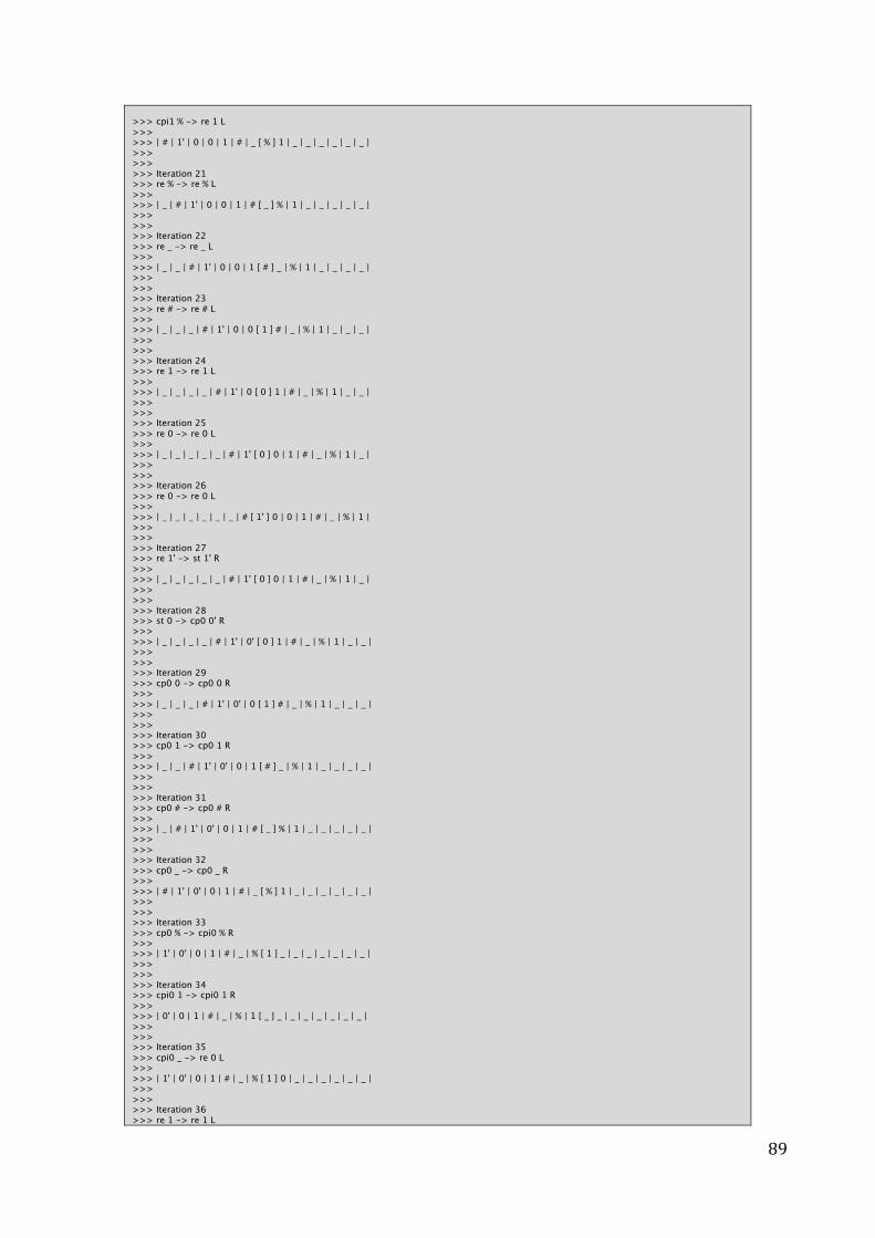
89

>>> cpi1 % -> re 1 L >>> >>> | # | 1' | 0 | 0 | 1 | # | _ [ % ] 1 | _ | _ | _ | _ | _ | _ | >>> >>> >>> Iteration 21 >>> re % -> re % L >>> >>> | _ | # | 1' | 0 | 0 | 1 | # [ _ ] % | 1 | _ | _ | _ | _ | _ | >>> >>> >>> Iteration 22 >>> re _ -> re _ L >>> >>> | _ | _ | # | 1' | 0 | 0 | 1 [ # ] _ | % | 1 | _ | _ | _ | _ | >>> >>> >>> Iteration 23 >>> re # -> re # L >>> >>> | _ | _ | _ | # | 1' | 0 | 0 [ 1 ] # | _ | % | 1 | _ | _ | _ | >>> >>> >>> Iteration 24 >>> re 1 -> re 1 L >>> >>> | _ | _ | _ | _ | # | 1' | 0 [ 0 ] 1 | # | _ | % | 1 | _ | _ | >>> >>> >>> Iteration 25 >>> re 0 -> re 0 L >>> >>> | _ | _ | _ | _ | _ | # | 1' [ 0 ] 0 | 1 | # | _ | % | 1 | _ | >>> >>> >>> Iteration 26 >>> re 0 -> re 0 L >>> >>> | _ | _ | _ | _ | _ | _ | # [ 1' ] 0 | 0 | 1 | # | _ | % | 1 | >>> >>> >>> Iteration 27 >>> re 1' -> st 1' R >>> >>> | _ | _ | _ | _ | _ | # | 1' [ 0 ] 0 | 1 | # | _ | % | 1 | _ | >>> >>> >>> Iteration 28 >>> st 0 -> cp0 0' R >>> >>> | _ | _ | _ | _ | # | 1' | 0' [ 0 ] 1 | # | _ | % | 1 | _ | _ | >>> >>> >>> Iteration 29 >>> cp0 0 -> cp0 0 R >>> >>> | _ | _ | _ | # | 1' | 0' | 0 [ 1 ] # | _ | % | 1 | _ | _ | _ | >>> >>> >>> Iteration 30 >>> cp0 1 -> cp0 1 R >>> >>> | _ | _ | # | 1' | 0' | 0 | 1 [ # ] _ | % | 1 | _ | _ | _ | _ | >>> >>> >>> Iteration 31 >>> cp0 # -> cp0 # R >>> >>> | _ | # | 1' | 0' | 0 | 1 | # [ _ ] % | 1 | _ | _ | _ | _ | _ | >>> >>> >>> Iteration 32 >>> cp0 _ -> cp0 _ R >>> >>> | # | 1' | 0' | 0 | 1 | # | _ [ % ] 1 | _ | _ | _ | _ | _ | _ | >>> >>> >>> Iteration 33 >>> cp0 % -> cpi0 % R >>> >>> | 1' | 0' | 0 | 1 | # | _ | % [ 1 ] _ | _ | _ | _ | _ | _ | _ | >>> >>> >>> Iteration 34 >>> cpi0 1 -> cpi0 1 R >>> >>> | 0' | 0 | 1 | # | _ | % | 1 [ _ ] _ | _ | _ | _ | _ | _ | _ | >>> >>> >>> Iteration 35 >>> cpi0 _ -> re 0 L >>> >>> | 1' | 0' | 0 | 1 | # | _ | % [ 1 ] 0 | _ | _ | _ | _ | _ | _ | >>> >>> >>> Iteration 36 >>> re 1 -> re 1 L

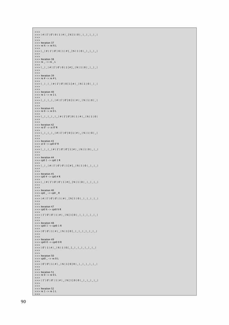
90

>>> >>> | # | 1' | 0' | 0 | 1 | # | _ [ % ] 1 | 0 | _ | _ | _ | _ | _ | >>> >>> >>> Iteration 37 >>> re % -> re % L >>> >>> | _ | # | 1' | 0' | 0 | 1 | # [ _ ] % | 1 | 0 | _ | _ | _ | _ | >>> >>> >>> Iteration 38 >>> re _ -> re _ L >>> >>> | _ | _ | # | 1' | 0' | 0 | 1 [ # ] _ | % | 1 | 0 | _ | _ | _ | >>> >>> >>> Iteration 39 >>> re # -> re # L >>> >>> | _ | _ | _ | # | 1' | 0' | 0 [ 1 ] # | _ | % | 1 | 0 | _ | _ | >>> >>> >>> Iteration 40 >>> re 1 -> re 1 L >>> >>> | _ | _ | _ | _ | # | 1' | 0' [ 0 ] 1 | # | _ | % | 1 | 0 | _ | >>> >>> >>> Iteration 41 >>> re 0 -> re 0 L >>> >>> | _ | _ | _ | _ | _ | # | 1' [ 0' ] 0 | 1 | # | _ | % | 1 | 0 | >>> >>> >>> Iteration 42 >>> re 0' -> st 0' R >>> >>> | _ | _ | _ | _ | # | 1' | 0' [ 0 ] 1 | # | _ | % | 1 | 0 | _ | >>> >>> >>> Iteration 43 >>> st 0 -> cp0 0' R >>> >>> | _ | _ | _ | # | 1' | 0' | 0' [ 1 ] # | _ | % | 1 | 0 | _ | _ | >>> >>> >>> Iteration 44 >>> cp0 1 -> cp0 1 R >>> >>> | _ | _ | # | 1' | 0' | 0' | 1 [ # ] _ | % | 1 | 0 | _ | _ | _ | >>> >>> >>> Iteration 45 >>> cp0 # -> cp0 # R >>> >>> | _ | # | 1' | 0' | 0' | 1 | # [ _ ] % | 1 | 0 | _ | _ | _ | _ | >>> >>> >>> Iteration 46 >>> cp0 _ -> cp0 _ R >>> >>> | # | 1' | 0' | 0' | 1 | # | _ [ % ] 1 | 0 | _ | _ | _ | _ | _ | >>> >>> >>> Iteration 47 >>> cp0 % -> cpi0 % R >>> >>> | 1' | 0' | 0' | 1 | # | _ | % [ 1 ] 0 | _ | _ | _ | _ | _ | _ | >>> >>> >>> Iteration 48 >>> cpi0 1 -> cpi0 1 R >>> >>> | 0' | 0' | 1 | # | _ | % | 1 [ 0 ] _ | _ | _ | _ | _ | _ | _ | >>> >>> >>> Iteration 49 >>> cpi0 0 -> cpi0 0 R >>> >>> | 0' | 1 | # | _ | % | 1 | 0 [ _ ] _ | _ | _ | _ | _ | _ | _ | >>> >>> >>> Iteration 50 >>> cpi0 _ -> re 0 L >>> >>> | 0' | 0' | 1 | # | _ | % | 1 [ 0 ] 0 | _ | _ | _ | _ | _ | _ | >>> >>> >>> Iteration 51 >>> re 0 -> re 0 L >>> >>> | 1' | 0' | 0' | 1 | # | _ | % [ 1 ] 0 | 0 | _ | _ | _ | _ | _ | >>> >>> >>> Iteration 52 >>> re 1 -> re 1 L >>>

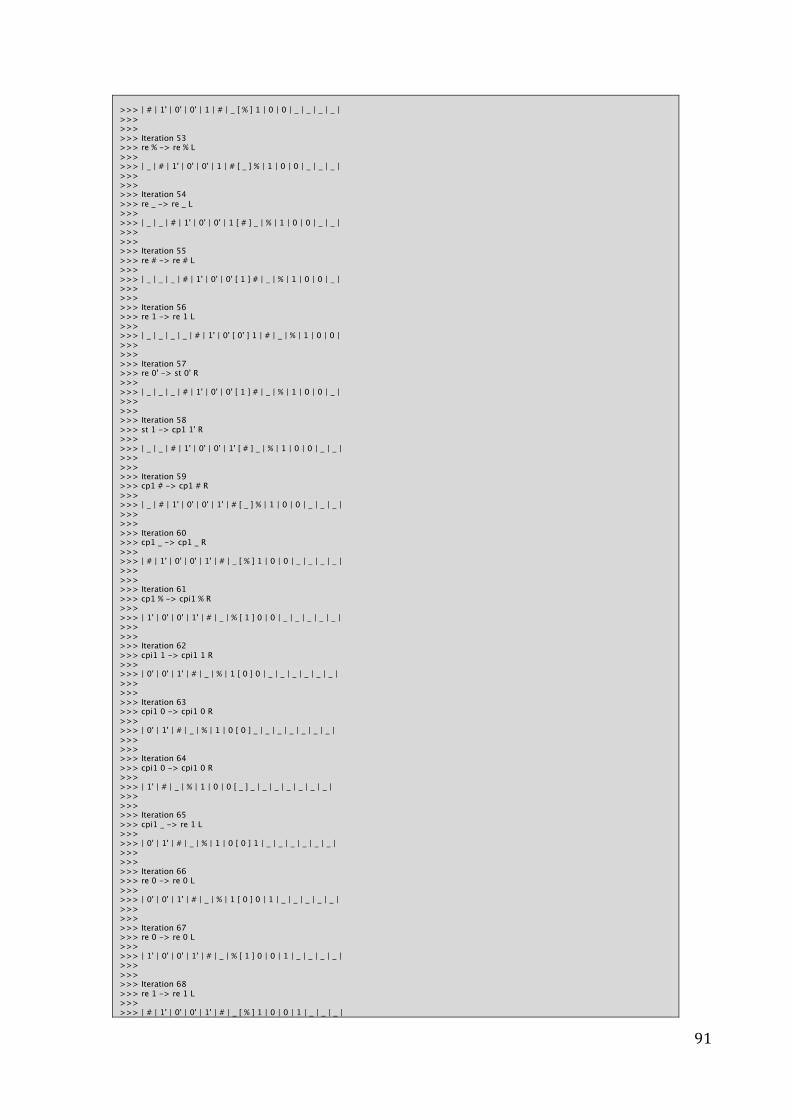
91

>>> | # | 1' | 0' | 0' | 1 | # | _ [ % ] 1 | 0 | 0 | _ | _ | _ | _ | >>> >>> >>> Iteration 53 >>> re % -> re % L >>> >>> | _ | # | 1' | 0' | 0' | 1 | # [ _ ] % | 1 | 0 | 0 | _ | _ | _ | >>> >>> >>> Iteration 54 >>> re _ -> re _ L >>> >>> | _ | _ | # | 1' | 0' | 0' | 1 [ # ] _ | % | 1 | 0 | 0 | _ | _ | >>> >>> >>> Iteration 55 >>> re # -> re # L >>> >>> | _ | _ | _ | # | 1' | 0' | 0' [ 1 ] # | _ | % | 1 | 0 | 0 | _ | >>> >>> >>> Iteration 56 >>> re 1 -> re 1 L >>> >>> | _ | _ | _ | _ | # | 1' | 0' [ 0' ] 1 | # | _ | % | 1 | 0 | 0 | >>> >>> >>> Iteration 57 >>> re 0' -> st 0' R >>> >>> | _ | _ | _ | # | 1' | 0' | 0' [ 1 ] # | _ | % | 1 | 0 | 0 | _ | >>> >>> >>> Iteration 58 >>> st 1 -> cp1 1' R >>> >>> | _ | _ | # | 1' | 0' | 0' | 1' [ # ] _ | % | 1 | 0 | 0 | _ | _ | >>> >>> >>> Iteration 59 >>> cp1 # -> cp1 # R >>> >>> | _ | # | 1' | 0' | 0' | 1' | # [ _ ] % | 1 | 0 | 0 | _ | _ | _ | >>> >>> >>> Iteration 60 >>> cp1 _ -> cp1 _ R >>> >>> | # | 1' | 0' | 0' | 1' | # | _ [ % ] 1 | 0 | 0 | _ | _ | _ | _ | >>> >>> >>> Iteration 61 >>> cp1 % -> cpi1 % R >>> >>> | 1' | 0' | 0' | 1' | # | _ | % [ 1 ] 0 | 0 | _ | _ | _ | _ | _ | >>> >>> >>> Iteration 62 >>> cpi1 1 -> cpi1 1 R >>> >>> | 0' | 0' | 1' | # | _ | % | 1 [ 0 ] 0 | _ | _ | _ | _ | _ | _ | >>> >>> >>> Iteration 63 >>> cpi1 0 -> cpi1 0 R >>> >>> | 0' | 1' | # | _ | % | 1 | 0 [ 0 ] _ | _ | _ | _ | _ | _ | _ | >>> >>> >>> Iteration 64 >>> cpi1 0 -> cpi1 0 R >>> >>> | 1' | # | _ | % | 1 | 0 | 0 [ _ ] _ | _ | _ | _ | _ | _ | _ | >>> >>> >>> Iteration 65 >>> cpi1 _ -> re 1 L >>> >>> | 0' | 1' | # | _ | % | 1 | 0 [ 0 ] 1 | _ | _ | _ | _ | _ | _ | >>> >>> >>> Iteration 66 >>> re 0 -> re 0 L >>> >>> | 0' | 0' | 1' | # | _ | % | 1 [ 0 ] 0 | 1 | _ | _ | _ | _ | _ | >>> >>> >>> Iteration 67 >>> re 0 -> re 0 L >>> >>> | 1' | 0' | 0' | 1' | # | _ | % [ 1 ] 0 | 0 | 1 | _ | _ | _ | _ | >>> >>> >>> Iteration 68 >>> re 1 -> re 1 L >>> >>> | # | 1' | 0' | 0' | 1' | # | _ [ % ] 1 | 0 | 0 | 1 | _ | _ | _ |

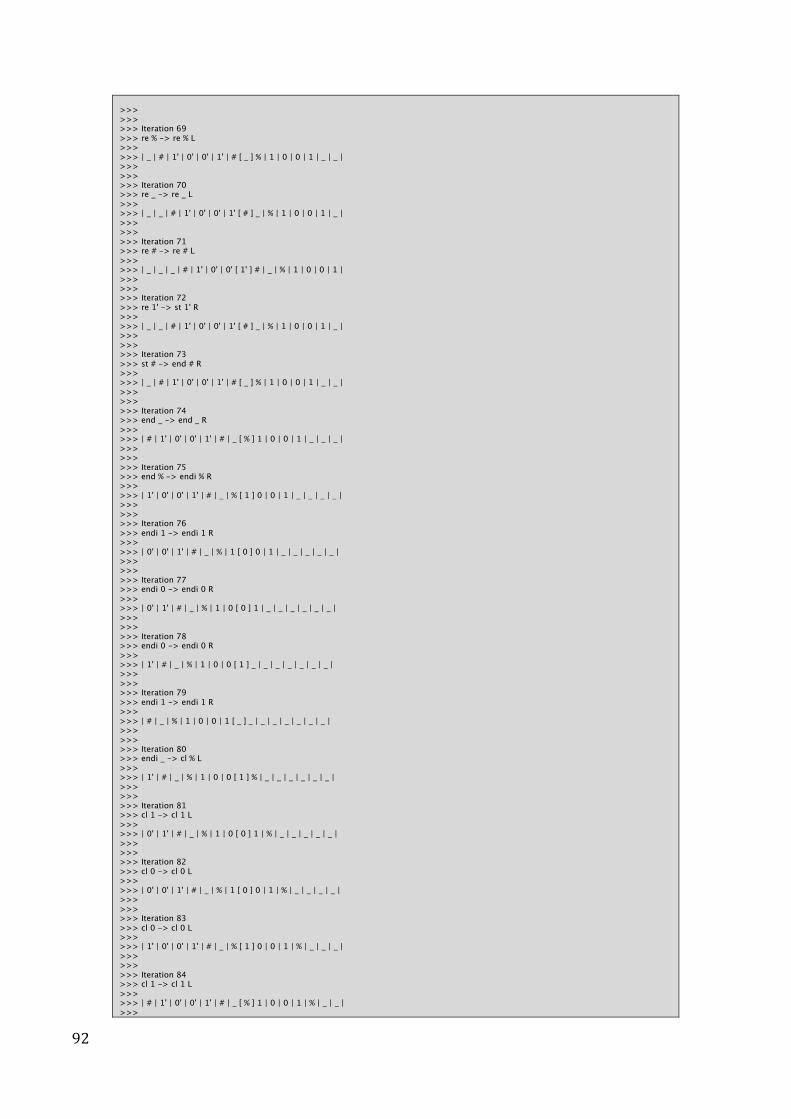
92

>>> >>> >>> Iteration 69 >>> re % -> re % L >>> >>> | _ | # | 1' | 0' | 0' | 1' | # [ _ ] % | 1 | 0 | 0 | 1 | _ | _ | >>> >>> >>> Iteration 70 >>> re _ -> re _ L >>> >>> | _ | _ | # | 1' | 0' | 0' | 1' [ # ] _ | % | 1 | 0 | 0 | 1 | _ | >>> >>> >>> Iteration 71 >>> re # -> re # L >>> >>> | _ | _ | _ | # | 1' | 0' | 0' [ 1' ] # | _ | % | 1 | 0 | 0 | 1 | >>> >>> >>> Iteration 72 >>> re 1' -> st 1' R >>> >>> | _ | _ | # | 1' | 0' | 0' | 1' [ # ] _ | % | 1 | 0 | 0 | 1 | _ | >>> >>> >>> Iteration 73 >>> st # -> end # R >>> >>> | _ | # | 1' | 0' | 0' | 1' | # [ _ ] % | 1 | 0 | 0 | 1 | _ | _ | >>> >>> >>> Iteration 74 >>> end _ -> end _ R >>> >>> | # | 1' | 0' | 0' | 1' | # | _ [ % ] 1 | 0 | 0 | 1 | _ | _ | _ | >>> >>> >>> Iteration 75 >>> end % -> endi % R >>> >>> | 1' | 0' | 0' | 1' | # | _ | % [ 1 ] 0 | 0 | 1 | _ | _ | _ | _ | >>> >>> >>> Iteration 76 >>> endi 1 -> endi 1 R >>> >>> | 0' | 0' | 1' | # | _ | % | 1 [ 0 ] 0 | 1 | _ | _ | _ | _ | _ | >>> >>> >>> Iteration 77 >>> endi 0 -> endi 0 R >>> >>> | 0' | 1' | # | _ | % | 1 | 0 [ 0 ] 1 | _ | _ | _ | _ | _ | _ | >>> >>> >>> Iteration 78 >>> endi 0 -> endi 0 R >>> >>> | 1' | # | _ | % | 1 | 0 | 0 [ 1 ] _ | _ | _ | _ | _ | _ | _ | >>> >>> >>> Iteration 79 >>> endi 1 -> endi 1 R >>> >>> | # | _ | % | 1 | 0 | 0 | 1 [ _ ] _ | _ | _ | _ | _ | _ | _ | >>> >>> >>> Iteration 80 >>> endi _ -> cl % L >>> >>> | 1' | # | _ | % | 1 | 0 | 0 [ 1 ] % | _ | _ | _ | _ | _ | _ | >>> >>> >>> Iteration 81 >>> cl 1 -> cl 1 L >>> >>> | 0' | 1' | # | _ | % | 1 | 0 [ 0 ] 1 | % | _ | _ | _ | _ | _ | >>> >>> >>> Iteration 82 >>> cl 0 -> cl 0 L >>> >>> | 0' | 0' | 1' | # | _ | % | 1 [ 0 ] 0 | 1 | % | _ | _ | _ | _ | >>> >>> >>> Iteration 83 >>> cl 0 -> cl 0 L >>> >>> | 1' | 0' | 0' | 1' | # | _ | % [ 1 ] 0 | 0 | 1 | % | _ | _ | _ | >>> >>> >>> Iteration 84 >>> cl 1 -> cl 1 L >>> >>> | # | 1' | 0' | 0' | 1' | # | _ [ % ] 1 | 0 | 0 | 1 | % | _ | _ | >>>

93

>>> >>> Iteration 85 >>> cl % -> cl % L >>> >>> | _ | # | 1' | 0' | 0' | 1' | # [ _ ] % | 1 | 0 | 0 | 1 | % | _ | >>> >>> >>> Iteration 86 >>> cl _ -> cl _ L >>> >>> | _ | _ | # | 1' | 0' | 0' | 1' [ # ] _ | % | 1 | 0 | 0 | 1 | % | >>> >>> >>> Iteration 87 >>> cl # -> cli # L >>> >>> | _ | _ | _ | # | 1' | 0' | 0' [ 1' ] # | _ | % | 1 | 0 | 0 | 1 | >>> >>> >>> Iteration 88 >>> cli 1' -> cli 1 L >>> >>> | _ | _ | _ | _ | # | 1' | 0' [ 0' ] 1 | # | _ | % | 1 | 0 | 0 | >>> >>> >>> Iteration 89 >>> cli 0' -> cli 0 L >>> >>> | _ | _ | _ | _ | _ | # | 1' [ 0' ] 0 | 1 | # | _ | % | 1 | 0 | >>> >>> >>> Iteration 90 >>> cli 0' -> cli 0 L >>> >>> | _ | _ | _ | _ | _ | _ | # [ 1' ] 0 | 0 | 1 | # | _ | % | 1 | >>> >>> >>> Iteration 91 >>> cli 1' -> cli 1 L >>> >>> | _ | _ | _ | _ | _ | _ | _ [ # ] 1 | 0 | 0 | 1 | # | _ | % | >>> >>> >>> Iteration 92 >>> cli # -> q3 # R >>> >>> | _ | _ | _ | _ | _ | _ | # [ 1 ] 0 | 0 | 1 | # | _ | % | 1 | >>> >>> >>> Iteration 93 >>> q3 1 -> q3 1 L >>> >>> | _ | _ | _ | _ | _ | _ | _ [ # ] 1 | 0 | 0 | 1 | # | _ | % | >>> >>> >>> Iteration 94 >>> q3 # -> q3 # L >>> >>> | _ | _ | _ | _ | _ | _ | _ [ _ ] # | 1 | 0 | 0 | 1 | # | _ | >>> >>> >>> Iteration 95 >>> q3 _ -> st1 _ R >>> >>> | _ | _ | _ | _ | _ | _ | _ [ # ] 1 | 0 | 0 | 1 | # | _ | % | >>> >>> >>> Iteration 96 >>> st1 # -> re1 # L >>> >>> | _ | _ | _ | _ | _ | _ | _ [ _ ] # | 1 | 0 | 0 | 1 | # | _ | >>> >>> >>> Iteration 97 >>> re1 _ -> rw7 _ R >>> >>> | _ | _ | _ | _ | _ | _ | _ [ # ] 1 | 0 | 0 | 1 | # | _ | % | >>> >>> >>> Iteration 98 >>> rw7 # -> st1 _ R >>> >>> | _ | _ | _ | _ | _ | _ | _ [ 1 ] 0 | 0 | 1 | # | _ | % | 1 | >>> >>> >>> Iteration 99 >>> st1 1 -> st1 1 R >>> >>> | _ | _ | _ | _ | _ | _ | 1 [ 0 ] 0 | 1 | # | _ | % | 1 | 0 | >>> >>> >>> Iteration 100 >>> st1 0 -> st1 0 R >>> >>> | _ | _ | _ | _ | _ | 1 | 0 [ 0 ] 1 | # | _ | % | 1 | 0 | 0 | >>> >>>

94

>>> Iteration 101 >>> st1 0 -> st1 0 R >>> >>> | _ | _ | _ | _ | 1 | 0 | 0 [ 1 ] # | _ | % | 1 | 0 | 0 | 1 | >>> >>> >>> Iteration 102 >>> st1 1 -> st1 1 R >>> >>> | _ | _ | _ | 1 | 0 | 0 | 1 [ # ] _ | % | 1 | 0 | 0 | 1 | % | >>> >>> >>> Iteration 103 >>> st1 # -> re1 # L >>> >>> | _ | _ | _ | _ | 1 | 0 | 0 [ 1 ] # | _ | % | 1 | 0 | 0 | 1 | >>> >>> >>> Iteration 104 >>> re1 1 -> re1 1 L >>> >>> | _ | _ | _ | _ | _ | 1 | 0 [ 0 ] 1 | # | _ | % | 1 | 0 | 0 | >>> >>> >>> Iteration 105 >>> re1 0 -> re1 0 L >>> >>> | _ | _ | _ | _ | _ | _ | 1 [ 0 ] 0 | 1 | # | _ | % | 1 | 0 | >>> >>> >>> Iteration 106 >>> re1 0 -> re1 0 L >>> >>> | _ | _ | _ | _ | _ | _ | _ [ 1 ] 0 | 0 | 1 | # | _ | % | 1 | >>> >>> >>> Iteration 107 >>> re1 1 -> re1 1 L >>> >>> | _ | _ | _ | _ | _ | _ | _ [ _ ] 1 | 0 | 0 | 1 | # | _ | % | >>> >>> >>> Iteration 108 >>> re1 _ -> rw7 _ R >>> >>> | _ | _ | _ | _ | _ | _ | _ [ 1 ] 0 | 0 | 1 | # | _ | % | 1 | >>> >>> >>> Iteration 109 >>> rw7 1 -> rw1 _ R >>> >>> | _ | _ | _ | _ | _ | _ | _ [ 0 ] 0 | 1 | # | _ | % | 1 | 0 | >>> >>> >>> Iteration 110 >>> rw1 0 -> rw0 1 R >>> >>> | _ | _ | _ | _ | _ | _ | 1 [ 0 ] 1 | # | _ | % | 1 | 0 | 0 | >>> >>> >>> Iteration 111 >>> rw0 0 -> rw0 0 R >>> >>> | _ | _ | _ | _ | _ | 1 | 0 [ 1 ] # | _ | % | 1 | 0 | 0 | 1 | >>> >>> >>> Iteration 112 >>> rw0 1 -> rw1 0 R >>> >>> | _ | _ | _ | _ | 1 | 0 | 0 [ # ] _ | % | 1 | 0 | 0 | 1 | % | >>> >>> >>> Iteration 113 >>> rw1 # -> st1 1 R >>> >>> | _ | _ | _ | 1 | 0 | 0 | 1 [ _ ] % | 1 | 0 | 0 | 1 | % | _ | >>> >>> >>> Iteration 114 >>> st1 _ -> q4 _ L >>> >>> | _ | _ | _ | _ | 1 | 0 | 0 [ 1 ] _ | % | 1 | 0 | 0 | 1 | % | >>> >>> >>> Iteration 115 >>> q4 1 -> q4 1 L >>> >>> | _ | _ | _ | _ | _ | 1 | 0 [ 0 ] 1 | _ | % | 1 | 0 | 0 | 1 | >>> >>> >>> Iteration 116 >>> q4 0 -> q4 0 L >>> >>> | _ | _ | _ | _ | _ | _ | 1 [ 0 ] 0 | 1 | _ | % | 1 | 0 | 0 | >>> >>> >>> Iteration 117

95

>>> q4 0 -> q4 0 L >>> >>> | _ | _ | _ | _ | _ | _ | _ [ 1 ] 0 | 0 | 1 | _ | % | 1 | 0 | >>> >>> >>> Iteration 118 >>> q4 1 -> q4 1 L >>> >>> | _ | _ | _ | _ | _ | _ | _ [ _ ] 1 | 0 | 0 | 1 | _ | % | 1 | >>> >>> >>> Iteration 119 >>> q4 _ -> q5 _ R >>> >>> | _ | _ | _ | _ | _ | _ | _ [ 1 ] 0 | 0 | 1 | _ | % | 1 | 0 | >>> >>> >>> Iteration 120 >>> q5 1 -> s1 _ R >>> >>> | _ | _ | _ | _ | _ | _ | _ [ 0 ] 0 | 1 | _ | % | 1 | 0 | 0 | >>> >>> >>> Iteration 121 >>> s1 0 -> s1 0 R >>> >>> | _ | _ | _ | _ | _ | _ | 0 [ 0 ] 1 | _ | % | 1 | 0 | 0 | 1 | >>> >>> >>> Iteration 122 >>> s1 0 -> s1 0 R >>> >>> | _ | _ | _ | _ | _ | 0 | 0 [ 1 ] _ | % | 1 | 0 | 0 | 1 | % | >>> >>> >>> Iteration 123 >>> s1 1 -> s1 1 R >>> >>> | _ | _ | _ | _ | 0 | 0 | 1 [ _ ] % | 1 | 0 | 0 | 1 | % | _ | >>> >>> >>> Iteration 124 >>> s1 _ -> c1 _ L >>> >>> | _ | _ | _ | _ | _ | 0 | 0 [ 1 ] _ | % | 1 | 0 | 0 | 1 | % | >>> >>> >>> Iteration 125 >>> c1 1 -> r _ L >>> >>> | _ | _ | _ | _ | _ | _ | 0 [ 0 ] _ | _ | % | 1 | 0 | 0 | 1 | >>> >>> >>> Iteration 126 >>> r 0 -> r 0 L >>> >>> | _ | _ | _ | _ | _ | _ | _ [ 0 ] 0 | _ | _ | % | 1 | 0 | 0 | >>> >>> >>> Iteration 127 >>> r 0 -> r 0 L >>> >>> | _ | _ | _ | _ | _ | _ | _ [ _ ] 0 | 0 | _ | _ | % | 1 | 0 | >>> >>> >>> Iteration 128 >>> r _ -> q5 _ R >>> >>> | _ | _ | _ | _ | _ | _ | _ [ 0 ] 0 | _ | _ | % | 1 | 0 | 0 | >>> >>> >>> Iteration 129 >>> q5 0 -> s0 _ R >>> >>> | _ | _ | _ | _ | _ | _ | _ [ 0 ] _ | _ | % | 1 | 0 | 0 | 1 | >>> >>> >>> Iteration 130 >>> s0 0 -> s0 0 R >>> >>> | _ | _ | _ | _ | _ | _ | 0 [ _ ] _ | % | 1 | 0 | 0 | 1 | % | >>> >>> >>> Iteration 131 >>> s0 _ -> c0 _ L >>> >>> | _ | _ | _ | _ | _ | _ | _ [ 0 ] _ | _ | % | 1 | 0 | 0 | 1 | >>> >>> >>> Iteration 132 >>> c0 0 -> r _ L >>> >>> | _ | _ | _ | _ | _ | _ | _ [ _ ] _ | _ | _ | % | 1 | 0 | 0 | >>> >>> >>> Iteration 133 >>> r _ -> q5 _ R

96

>>> >>> | _ | _ | _ | _ | _ | _ | _ [ _ ] _ | _ | % | 1 | 0 | 0 | 1 | >>> >>> >>> Iteration 134 >>> q5 _ -> q+ _ R >>> >>> | _ | _ | _ | _ | _ | _ | _ [ _ ] _ | _ | % | 1 | 0 | 0 | 1 | >>> >>> Length of initial tape: 8 >>> Length of final tape: 8 >>> Maximum length of tape: 14 >>> Configurations generated: 134 >>> >>>

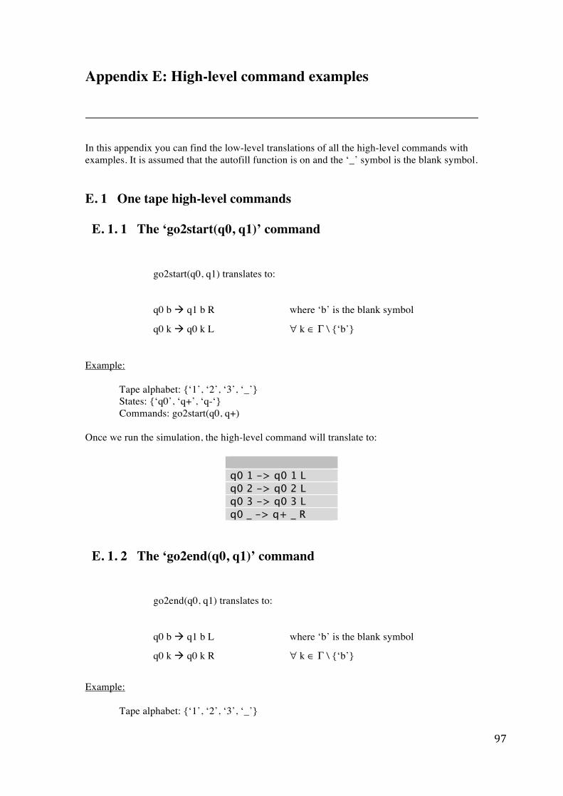
97

Appendix E: High-level command examples

In this appendix you can find the low-level translations of all the high-level commands with examples. It is assumed that the autofill function is on and the ‘_’ symbol is the blank symbol.

E. 1 One tape high-level commands E. 1. 1 The ‘go2start(q0, q1)’ command


q0 b q1 b R where ‘b’ is the blank symbol

q0 k q0 k L ∀ k ∈ Γ \ {‘b’} Example: Tape alphabet: {‘1’, ‘2’, ‘3’, ‘_’} States: {‘q0’, ‘q+’, ‘q-‘}

Commands: go2start(q0, q+)

Once we run the simulation, the high-level command will translate to:

q0 1 -> q0 1 L q0 2 -> q0 2 L q0 3 -> q0 3 L q0 _ -> q+ _ R

E. 1. 2 The ‘go2end(q0, q1)’ command


q0 b q1 b L where ‘b’ is the blank symbol

q0 k q0 k R ∀ k ∈ Γ \ {‘b’}

Example: Tape alphabet: {‘1’, ‘2’, ‘3’, ‘_’}

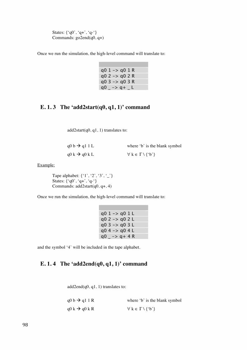
98

States: {‘q0’, ‘q+’, ‘q-‘} Commands: go2end(q0, q+)


q0 1 -> q0 1 R q0 2 -> q0 2 R q0 3 -> q0 3 R q0 _ -> q+ _ L

E. 1. 3 The ‘add2start(q0, q1, 1)’ command

add2start(q0, q1, 1) translates to:

q0 b q1 1 L where ‘b’ is the blank symbol

q0 k q0 k L ∀ k ∈ Γ \ {‘b’}

Example: Tape alphabet: {‘1’, ‘2’, ‘3’, ‘_’} States: {‘q0’, ‘q+’, ‘q-‘}

Commands: add2start(q0, q+, 4)


q0 1 -> q0 1 L q0 2 -> q0 2 L q0 3 -> q0 3 L q0 4 -> q0 4 L q0 _ -> q+ 4 R

and the symbol ‘4’ will be included in the tape alphabet. E. 1. 4 The ‘add2end(q0, q1, 1)’ command

add2end(q0, q1, 1) translates to:

q0 b q1 1 R where ‘b’ is the blank symbol

q0 k q0 k R ∀ k ∈ Γ \ {‘b’}

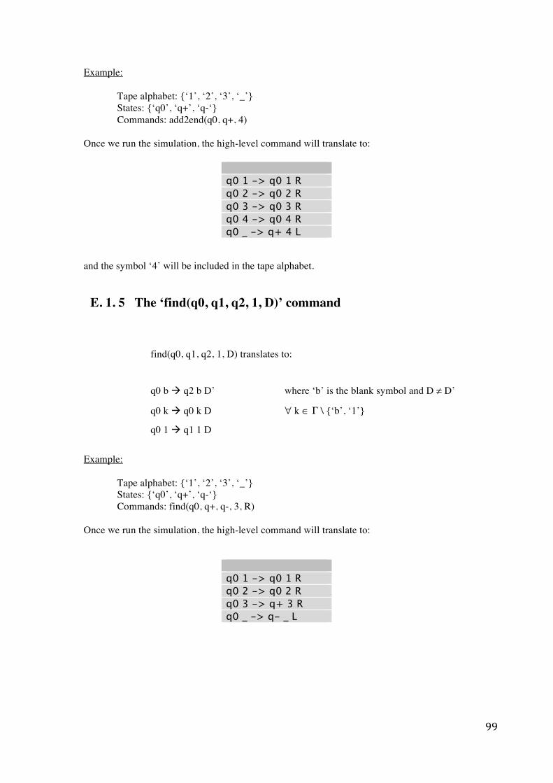
99


Commands: add2end(q0, q+, 4)


q0 1 -> q0 1 R q0 2 -> q0 2 R q0 3 -> q0 3 R q0 4 -> q0 4 R q0 _ -> q+ 4 L

and the symbol ‘4’ will be included in the tape alphabet. E. 1. 5 The ‘find(q0, q1, q2, 1, D)’ command

find(q0, q1, q2, 1, D) translates to:

q0 b q2 b D’ where ‘b’ is the blank symbol and D ≠ D’

q0 k q0 k D ∀ k ∈ Γ \ {‘b’, ‘1’}

q0 1 q1 1 D


Commands: find(q0, q+, q-, 3, R)


q0 1 -> q0 1 R q0 2 -> q0 2 R q0 3 -> q+ 3 R q0 _ -> q- _ L

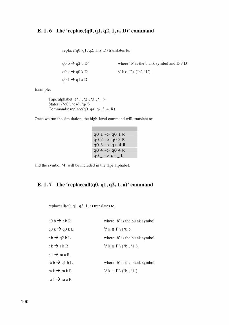
100

E. 1. 6 The ‘replace(q0, q1, q2, 1, a, D)’ command

replace(q0, q1, q2, 1, a, D) translates to:

q0 b q2 b D’ where ‘b’ is the blank symbol and D ≠ D’

q0 k q0 k D ∀ k ∈ Γ \ {‘b’, ‘1’}

q0 1 q1 a D


Commands: replace(q0, q+, q-, 3, 4, R)


q0 1 -> q0 1 R q0 2 -> q0 2 R q0 3 -> q+ 4 R q0 4 -> q0 4 R q0 _ -> q- _ L

and the symbol ‘4’ will be included in the tape alphabet.

E. 1. 7 The ‘replaceall(q0, q1, q2, 1, a)’ command

replaceall(q0, q1, q2, 1, a) translates to:

q0 b r b R where ‘b’ is the blank symbol

q0 k q0 k L ∀ k ∈ Γ \ {‘b’}

r b q2 b L where ‘b’ is the blank symbol

r k r k R ∀ k ∈ Γ \ {‘b’, ‘1’}

r 1 ra a R

ra b q1 b L where ‘b’ is the blank symbol

ra k ra k R ∀ k ∈ Γ \ {‘b’, ‘1’}

ra 1 ra a R

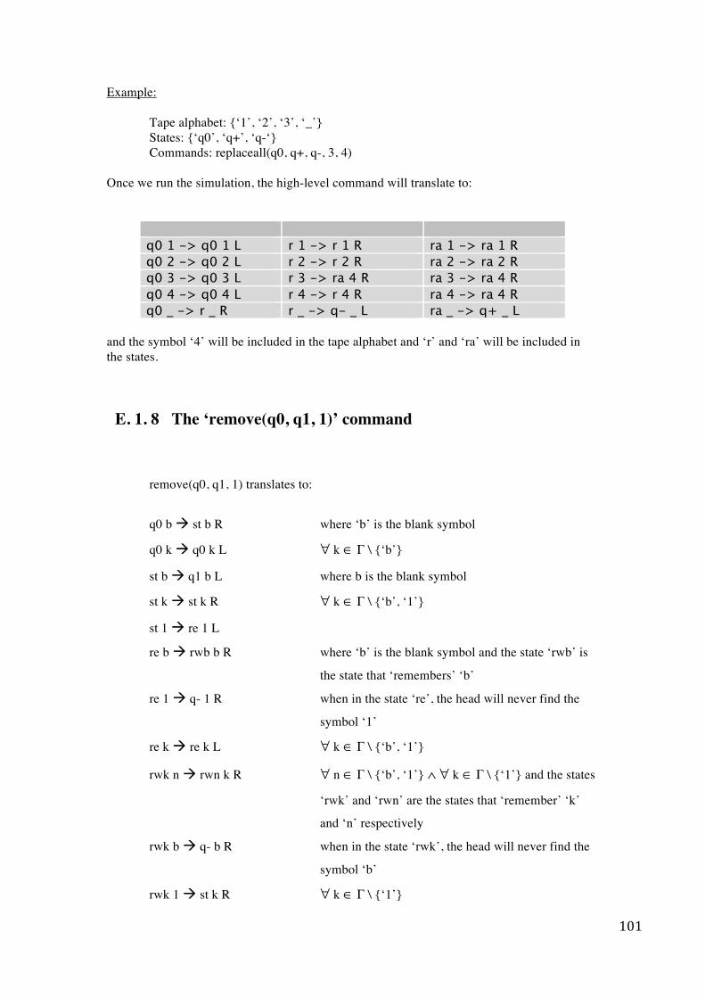
101


Commands: replaceall(q0, q+, q-, 3, 4)


q0 1 -> q0 1 L r 1 -> r 1 R ra 1 -> ra 1 R q0 2 -> q0 2 L r 2 -> r 2 R ra 2 -> ra 2 R q0 3 -> q0 3 L r 3 -> ra 4 R ra 3 -> ra 4 R q0 4 -> q0 4 L r 4 -> r 4 R ra 4 -> ra 4 R q0 _ -> r _ R r _ -> q- _ L ra _ -> q+ _ L

and the symbol ‘4’ will be included in the tape alphabet and ‘r’ and ‘ra’ will be included in the states.

E. 1. 8 The ‘remove(q0, q1, 1)’ command

remove(q0, q1, 1) translates to:

q0 b st b R where ‘b’ is the blank symbol

q0 k q0 k L ∀ k ∈ Γ \ {‘b’}

st b q1 b L where b is the blank symbol

st k st k R ∀ k ∈ Γ \ {‘b’, ‘1’}

st 1 re 1 L

re b rwb b R where ‘b’ is the blank symbol and the state ‘rwb’ is

the state that ‘remembers’ ‘b’

re 1 q- 1 R when in the state ‘re’, the head will never find the

symbol ‘1’

re k re k L ∀ k ∈ Γ \ {‘b’, ‘1’}

rwk n rwn k R ∀ n ∈ Γ \ {‘b’, ‘1’} ∧ ∀ k ∈ Γ \ {‘1’} and the states

‘rwk’ and ‘rwn’ are the states that ‘remember’ ‘k’

and ‘n’ respectively

rwk b q- b R when in the state ‘rwk’, the head will never find the

symbol ‘b’

rwk 1 st k R ∀ k ∈ Γ \ {‘1’}

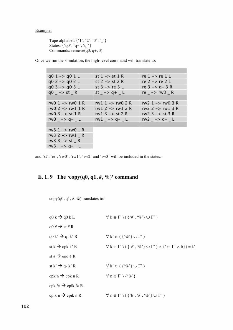
102


Commands: remove(q0, q+, 3) Once we run the simulation, the high-level command will translate to:

q0 1 -> q0 1 L st 1 -> st 1 R re 1 -> re 1 L q0 2 -> q0 2 L st 2 -> st 2 R re 2 -> re 2 L q0 3 -> q0 3 L st 3 -> re 3 L re 3 -> q- 3 R q0 _ -> st _ R st _ -> q+ _ L re _ -> rw3 _ R rw0 1 -> rw0 1 R rw1 1 -> rw0 2 R rw2 1 -> rw0 3 R rw0 2 -> rw1 1 R rw1 2 -> rw1 2 R rw2 2 -> rw1 3 R rw0 3 -> st 1 R rw1 3 -> st 2 R rw2 3 -> st 3 R rw0 _ -> q- _ L rw1 _ -> q- _ L rw2 _ -> q- _ L rw3 1 -> rw0 _ R rw3 2 -> rw1 _ R rw3 3 -> st _ R rw3 _ -> q- _ L

and ‘st’, ‘re’, ‘rw0’, ‘rw1’, ‘rw2’ and ‘rw3’ will be included in the states.

E. 1. 9 The ‘copy(q0, q1, #, %)’ command

copy(q0, q1, #, %) translates to:

q0 k q0 k L ∀ k ∈ Γ \ ( {‘#’, ‘%’} ∪ Γ’ )

q0 # st # R

q0 k’ q- k’ R ∀ k’ ∈ ( {‘%’} ∪ Γ’ )

st k cpk k’ R ∀ k ∈ Γ \ ( {‘#’, ‘%’} ∪ Γ’ ) ∧ k’ ∈ Γ’ ∧ f(k) = k’

st # end # R

st k’ q- k’ R ∀ k’ ∈ ( {‘%’} ∪ Γ’ )

cpk n cpk n R ∀ n ∈ Γ \ {‘%’}

cpk % cpik % R

cpik n cpik n R ∀ n ∈ Γ \ ( {‘b’, ‘#’, ‘%’} ∪ Γ’ )

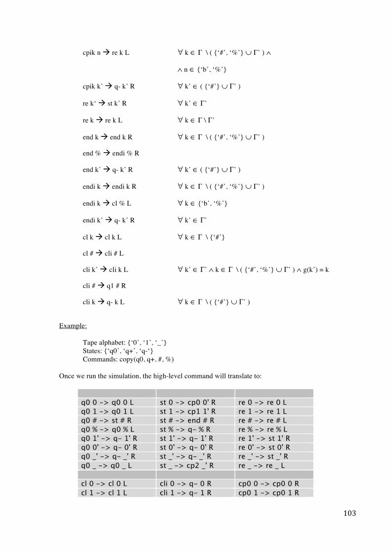
103

cpik n re k L ∀ k ∈ Γ \ ( {‘#’, ‘%’} ∪ Γ’ ) ∧

∧ n ∈ {‘b’, ‘%’}

cpik k’ q- k’ R ∀ k’ ∈ ( {‘#’} ∪ Γ’ )

re k‘ st k’ R ∀ k’ ∈ Γ’

re k re k L ∀ k ∈ Γ \ Γ’

end k end k R ∀ k ∈ Γ \ ( {‘#’, ‘%’} ∪ Γ’ )

end % endi % R

end k’ q- k’ R ∀ k’ ∈ ( {‘#’} ∪ Γ’ )

endi k endi k R ∀ k ∈ Γ \ ( {‘#’, ‘%’} ∪ Γ’ )

endi k cl % L ∀ k ∈ {‘b’, ‘%’}

endi k’ q- k’ R ∀ k’ ∈ Γ’

cl k cl k L ∀ k ∈ Γ \ {‘#’}

cl # cli # L

cli k’ cli k L ∀ k’ ∈ Γ’ ∧ k ∈ Γ \ ( {‘#’, ‘%’} ∪ Γ’ ) ∧ g(k’) = k

cli # q1 # R

cli k q- k L ∀ k ∈ Γ \ ( {‘#’} ∪ Γ’ )

Example: Tape alphabet: {‘0’, ‘1’, ‘_’} States: {‘q0’, ‘q+’, ‘q-‘}

Commands: copy(q0, q+, #, %)


q0 0 -> q0 0 L st 0 -> cp0 0' R re 0 -> re 0 L q0 1 -> q0 1 L st 1 -> cp1 1' R re 1 -> re 1 L q0 # -> st # R st # -> end # R re # -> re # L q0 % -> q0 % L st % -> q- % R re % -> re % L q0 1' -> q- 1' R st 1' -> q- 1' R re 1' -> st 1' R q0 0' -> q- 0' R st 0' -> q- 0' R re 0' -> st 0' R q0 _' -> q- _' R st _' -> q- _' R re _' -> st _' R q0 _ -> q0 _ L st _ -> cp2 _' R re _ -> re _ L cl 0 -> cl 0 L cli 0 -> q- 0 R cp0 0 -> cp0 0 R cl 1 -> cl 1 L cli 1 -> q- 1 R cp0 1 -> cp0 1 R

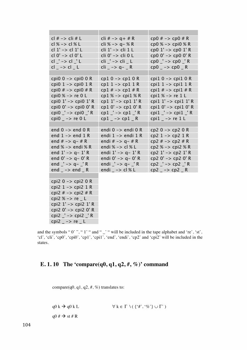
104

cl # -> cli # L cli # -> q+ # R cp0 # -> cp0 # R cl % -> cl % L cli % -> q- % R cp0 % -> cpi0 % R cl 1' -> cl 1' L cli 1' -> cli 1 L cp0 1' -> cp0 1' R cl 0' -> cl 0' L cli 0' -> cli 0 L cp0 0' -> cp0 0' R cl _' -> cl _' L cli _' -> cli _ L cp0 _' -> cp0 _' R cl _ -> cl _ L cli _ -> q- _ R cp0 _ -> cp0 _ R cpi0 0 -> cpi0 0 R cp1 0 -> cp1 0 R cpi1 0 -> cpi1 0 R cpi0 1 -> cpi0 1 R cp1 1 -> cp1 1 R cpi1 1 -> cpi1 1 R cpi0 # -> cpi0 # R cp1 # -> cp1 # R cpi1 # -> cpi1 # R cpi0 % -> re 0 L cp1 % -> cpi1 % R cpi1 % -> re 1 L cpi0 1' -> cpi0 1' R cp1 1' -> cp1 1' R cpi1 1' -> cpi1 1' R cpi0 0' -> cpi0 0' R cp1 0' -> cp1 0' R cpi1 0' -> cpi1 0' R cpi0 _' -> cpi0 _' R cp1 _' -> cp1 _' R cpi1 _' -> cpi1 _' R cpi0 _ -> re 0 L cp1 _ -> cp1 _ R cpi1 _ -> re 1 L end 0 -> end 0 R endi 0 -> endi 0 R cp2 0 -> cp2 0 R end 1 -> end 1 R endi 1 -> endi 1 R cp2 1 -> cp2 1 R end # -> q- # R endi # -> q- # R cp2 # -> cp2 # R end % -> endi % R endi % -> cl % L cp2 % -> cpi2 % R end 1' -> q- 1' R endi 1' -> q- 1' R cp2 1' -> cp2 1' R end 0' -> q- 0' R endi 0' -> q- 0' R cp2 0' -> cp2 0' R end _' -> q- _' R endi _' -> q- _' R cp2 _' -> cp2 _' R end _ -> end _ R endi _ -> cl % L cp2 _ -> cp2 _ R cpi2 0 -> cpi2 0 R cpi2 1 -> cpi2 1 R cpi2 # -> cpi2 # R cpi2 % -> re _ L cpi2 1' -> cpi2 1' R cpi2 0' -> cpi2 0' R cpi2 _' -> cpi2 _' R cpi2 _ -> re _ L

and the symbols “ 0’ ”, “ 1’ “ and “ _’ “ will be included in the tape alphabet and ‘re’, ‘st’, ‘cl’, ‘cli’, ‘cp0’, ‘cpi0’, ‘cp1’, ‘cpi1’, ‘end’, ‘endi’, ‘cp2’ and ‘cpi2’ will be included in the states.

E. 1. 10 The ‘compare(q0, q1, q2, #, %)’ command

compare(q0, q1, q2, #, %) translates to:

q0 k q0 k L ∀ k ∈ Γ \ ( {‘#’, ‘%’} ∪ Γ’ )

q0 # st # R

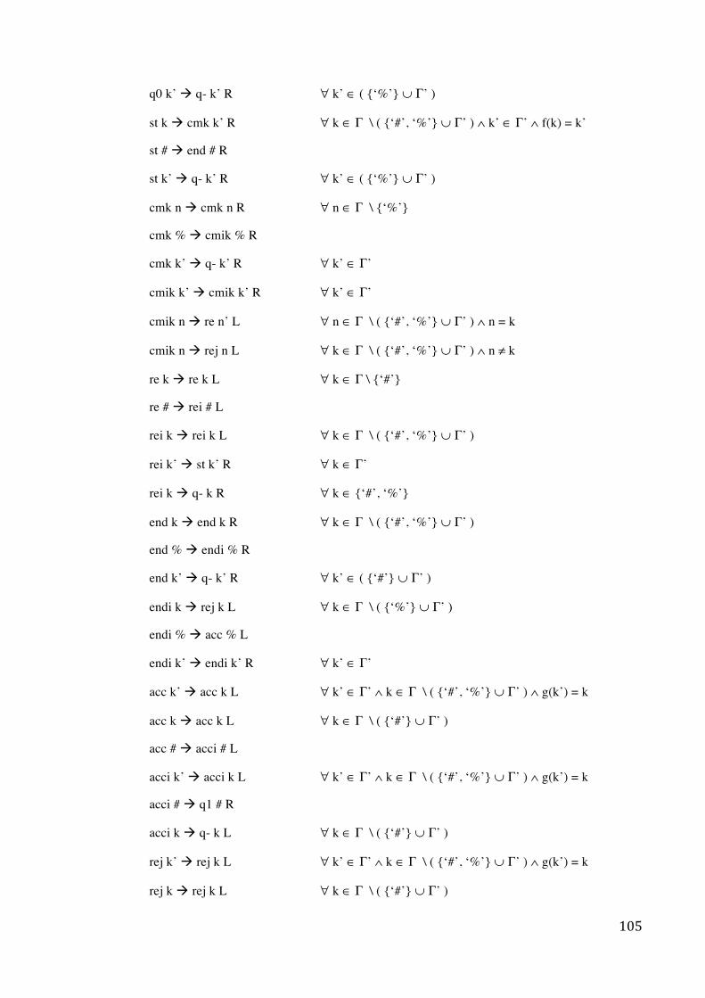
105

q0 k’ q- k’ R ∀ k’ ∈ ( {‘%’} ∪ Γ’ )

st k cmk k’ R ∀ k ∈ Γ \ ( {‘#’, ‘%’} ∪ Γ’ ) ∧ k’ ∈ Γ’ ∧ f(k) = k’

st # end # R

st k’ q- k’ R ∀ k’ ∈ ( {‘%’} ∪ Γ’ )

cmk n cmk n R ∀ n ∈ Γ \ {‘%’}

cmk % cmik % R

cmk k’ q- k’ R ∀ k’ ∈ Γ’

cmik k’ cmik k’ R ∀ k’ ∈ Γ’

cmik n re n’ L ∀ n ∈ Γ \ ( {‘#’, ‘%’} ∪ Γ’ ) ∧ n = k

cmik n rej n L ∀ k ∈ Γ \ ( {‘#’, ‘%’} ∪ Γ’ ) ∧ n ≠ k

re k re k L ∀ k ∈ Γ \ {‘#’}

re # rei # L

rei k rei k L ∀ k ∈ Γ \ ( {‘#’, ‘%’} ∪ Γ’ )

rei k’ st k’ R ∀ k ∈ Γ’

rei k q- k R ∀ k ∈ {‘#’, ‘%’}

end k end k R ∀ k ∈ Γ \ ( {‘#’, ‘%’} ∪ Γ’ )

end % endi % R

end k’ q- k’ R ∀ k’ ∈ ( {‘#’} ∪ Γ’ )

endi k rej k L ∀ k ∈ Γ \ ( {‘%’} ∪ Γ’ )

endi % acc % L

endi k’ endi k’ R ∀ k’ ∈ Γ’

acc k’ acc k L ∀ k’ ∈ Γ’ ∧ k ∈ Γ \ ( {‘#’, ‘%’} ∪ Γ’ ) ∧ g(k’) = k

acc k acc k L ∀ k ∈ Γ \ ( {‘#’} ∪ Γ’ )

acc # acci # L

acci k’ acci k L ∀ k’ ∈ Γ’ ∧ k ∈ Γ \ ( {‘#’, ‘%’} ∪ Γ’ ) ∧ g(k’) = k

acci # q1 # R

acci k q- k L ∀ k ∈ Γ \ ( {‘#’} ∪ Γ’ )

rej k’ rej k L ∀ k’ ∈ Γ’ ∧ k ∈ Γ \ ( {‘#’, ‘%’} ∪ Γ’ ) ∧ g(k’) = k

rej k rej k L ∀ k ∈ Γ \ ( {‘#’} ∪ Γ’ )

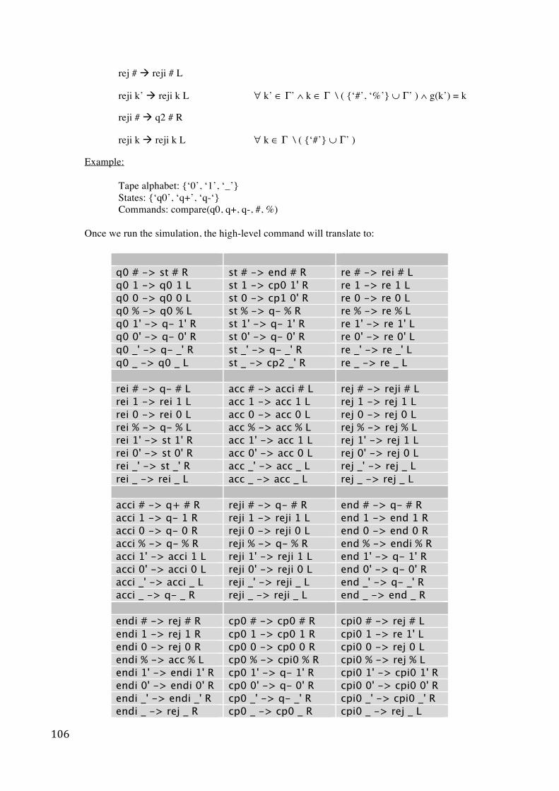
106

rej # reji # L

reji k’ reji k L ∀ k’ ∈ Γ’ ∧ k ∈ Γ \ ( {‘#’, ‘%’} ∪ Γ’ ) ∧ g(k’) = k

reji # q2 # R

reji k reji k L ∀ k ∈ Γ \ ( {‘#’} ∪ Γ’ )

Example: Tape alphabet: {‘0’, ‘1’, ‘_’} States: {‘q0’, ‘q+’, ‘q-‘}

Commands: compare(q0, q+, q-, #, %)


q0 # -> st # R st # -> end # R re # -> rei # L q0 1 -> q0 1 L st 1 -> cp0 1' R re 1 -> re 1 L q0 0 -> q0 0 L st 0 -> cp1 0' R re 0 -> re 0 L q0 % -> q0 % L st % -> q- % R re % -> re % L q0 1' -> q- 1' R st 1' -> q- 1' R re 1' -> re 1' L q0 0' -> q- 0' R st 0' -> q- 0' R re 0' -> re 0' L q0 _' -> q- _' R st _' -> q- _' R re _' -> re _' L q0 _ -> q0 _ L st _ -> cp2 _' R re _ -> re _ L rei # -> q- # L acc # -> acci # L rej # -> reji # L rei 1 -> rei 1 L acc 1 -> acc 1 L rej 1 -> rej 1 L rei 0 -> rei 0 L acc 0 -> acc 0 L rej 0 -> rej 0 L rei % -> q- % L acc % -> acc % L rej % -> rej % L rei 1' -> st 1' R acc 1' -> acc 1 L rej 1' -> rej 1 L rei 0' -> st 0' R acc 0' -> acc 0 L rej 0' -> rej 0 L rei _' -> st _' R acc _' -> acc _ L rej _' -> rej _ L rei _ -> rei _ L acc _ -> acc _ L rej _ -> rej _ L acci # -> q+ # R reji # -> q- # R end # -> q- # R acci 1 -> q- 1 R reji 1 -> reji 1 L end 1 -> end 1 R acci 0 -> q- 0 R reji 0 -> reji 0 L end 0 -> end 0 R acci % -> q- % R reji % -> q- % R end % -> endi % R acci 1' -> acci 1 L reji 1' -> reji 1 L end 1' -> q- 1' R acci 0' -> acci 0 L reji 0' -> reji 0 L end 0' -> q- 0' R acci _' -> acci _ L reji _' -> reji _ L end _' -> q- _' R acci _ -> q- _ R reji _ -> reji _ L end _ -> end _ R endi # -> rej # R cp0 # -> cp0 # R cpi0 # -> rej # L endi 1 -> rej 1 R cp0 1 -> cp0 1 R cpi0 1 -> re 1' L endi 0 -> rej 0 R cp0 0 -> cp0 0 R cpi0 0 -> rej 0 L endi % -> acc % L cp0 % -> cpi0 % R cpi0 % -> rej % L endi 1' -> endi 1' R cp0 1' -> q- 1' R cpi0 1' -> cpi0 1' R endi 0' -> endi 0' R cp0 0' -> q- 0' R cpi0 0' -> cpi0 0' R endi _' -> endi _' R cp0 _' -> q- _' R cpi0 _' -> cpi0 _' R endi _ -> rej _ R cp0 _ -> cp0 _ R cpi0 _ -> rej _ L

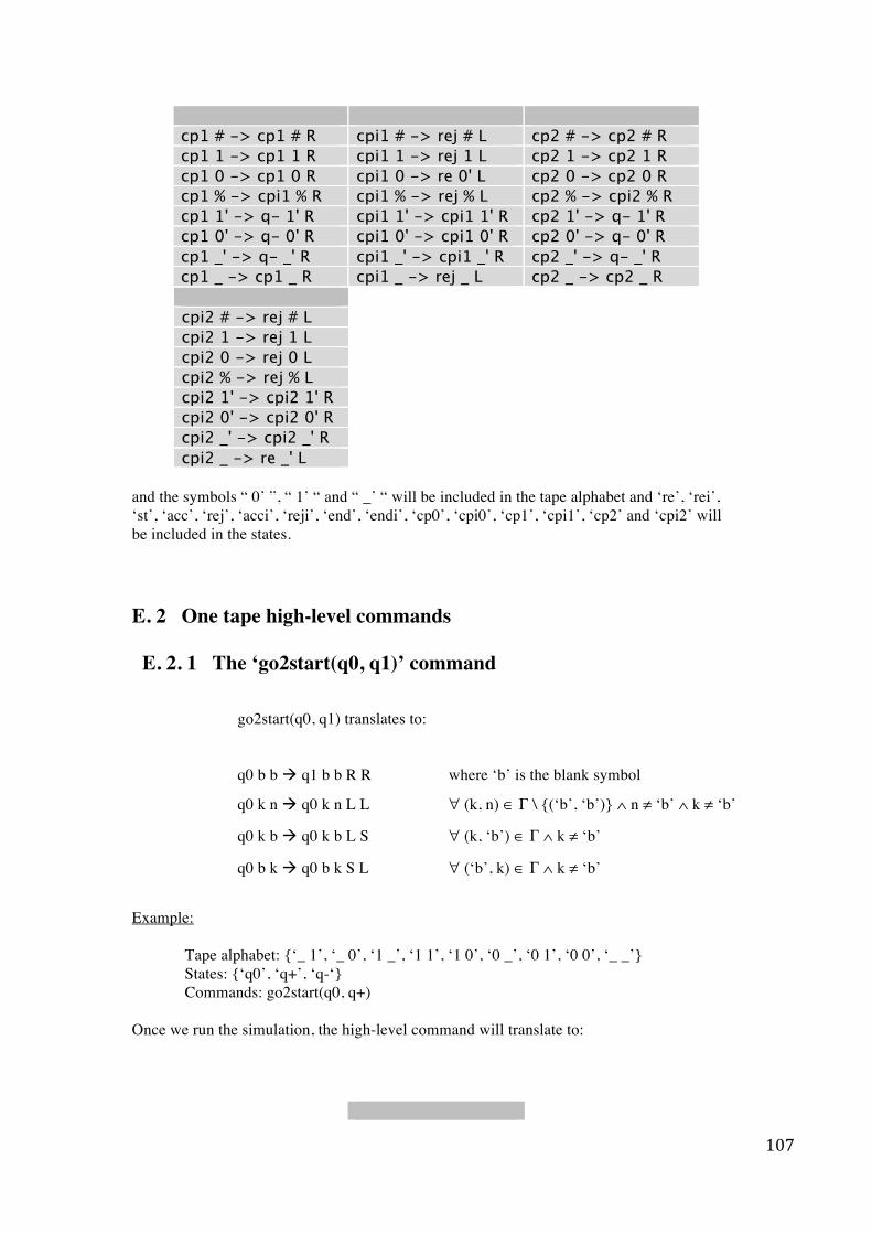
107

cp1 # -> cp1 # R cpi1 # -> rej # L cp2 # -> cp2 # R cp1 1 -> cp1 1 R cpi1 1 -> rej 1 L cp2 1 -> cp2 1 R cp1 0 -> cp1 0 R cpi1 0 -> re 0' L cp2 0 -> cp2 0 R cp1 % -> cpi1 % R cpi1 % -> rej % L cp2 % -> cpi2 % R cp1 1' -> q- 1' R cpi1 1' -> cpi1 1' R cp2 1' -> q- 1' R cp1 0' -> q- 0' R cpi1 0' -> cpi1 0' R cp2 0' -> q- 0' R cp1 _' -> q- _' R cpi1 _' -> cpi1 _' R cp2 _' -> q- _' R cp1 _ -> cp1 _ R cpi1 _ -> rej _ L cp2 _ -> cp2 _ R cpi2 # -> rej # L cpi2 1 -> rej 1 L cpi2 0 -> rej 0 L cpi2 % -> rej % L cpi2 1' -> cpi2 1' R cpi2 0' -> cpi2 0' R cpi2 _' -> cpi2 _' R cpi2 _ -> re _' L

and the symbols “ 0’ ”, “ 1’ “ and “ _’ “ will be included in the tape alphabet and ‘re’, ‘rei’, ‘st’, ‘acc’, ‘rej’, ‘acci’, ‘reji’, ‘end’, ‘endi’, ‘cp0’, ‘cpi0’, ‘cp1’, ‘cpi1’, ‘cp2’ and ‘cpi2’ will be included in the states. E. 2 One tape high-level commands E. 2. 1 The ‘go2start(q0, q1)’ command


q0 b b q1 b b R R where ‘b’ is the blank symbol


q0 k b q0 k b L S ∀ (k, ‘b’) ∈ Γ ∧ k ≠ ‘b’

q0 b k q0 b k S L ∀ (‘b’, k) ∈ Γ ∧ k ≠ ‘b’

Example: Tape alphabet: {‘_ 1’, ‘_ 0’, ‘1 _’, ‘1 1’, ‘1 0’, ‘0 _’, ‘0 1’, ‘0 0’, ‘_ _’} States: {‘q0’, ‘q+’, ‘q-‘}

Commands: go2start(q0, q+)


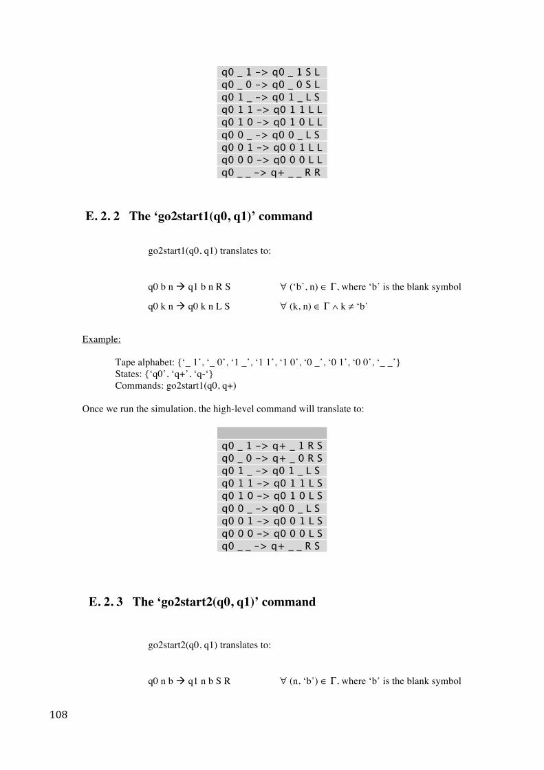
108

q0 _ 1 -> q0 _ 1 S L q0 _ 0 -> q0 _ 0 S L q0 1 _ -> q0 1 _ L S q0 1 1 -> q0 1 1 L L q0 1 0 -> q0 1 0 L L q0 0 _ -> q0 0 _ L S q0 0 1 -> q0 0 1 L L q0 0 0 -> q0 0 0 L L q0 _ _ -> q+ _ _ R R

E. 2. 2 The ‘go2start1(q0, q1)’ command


q0 b n q1 b n R S ∀ (‘b’, n) ∈ Γ, where ‘b’ is the blank symbol

q0 k n q0 k n L S ∀ (k, n) ∈ Γ ∧ k ≠ ‘b’


Commands: go2start1(q0, q+)


q0 _ 1 -> q+ _ 1 R S q0 _ 0 -> q+ _ 0 R S q0 1 _ -> q0 1 _ L S q0 1 1 -> q0 1 1 L S q0 1 0 -> q0 1 0 L S q0 0 _ -> q0 0 _ L S q0 0 1 -> q0 0 1 L S q0 0 0 -> q0 0 0 L S q0 _ _ -> q+ _ _ R S

E. 2. 3 The ‘go2start2(q0, q1)’ command


q0 n b q1 n b S R ∀ (n, ‘b’) ∈ Γ, where ‘b’ is the blank symbol

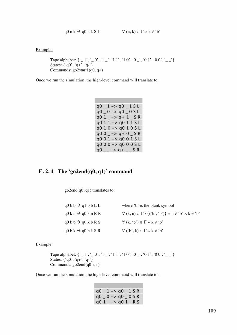
109

q0 n k q0 n k S L ∀ (n, k) ∈ Γ ∧ k ≠ ‘b’


Commands: go2start1(q0, q+) Once we run the simulation, the high-level command will translate to:

q0 _ 1 -> q0 _ 1 S L q0 _ 0 -> q0 _ 0 S L q0 1 _ -> q+ 1 _ S R q0 1 1 -> q0 1 1 S L q0 1 0 -> q0 1 0 S L q0 0 _ -> q+ 0 _ S R q0 0 1 -> q0 0 1 S L q0 0 0 -> q0 0 0 S L q0 _ _ -> q+ _ _ S R

E. 2. 4 The ‘go2end(q0, q1)’ command


q0 b b q1 b b L L where ‘b’ is the blank symbol

q0 k n q0 k n R R ∀ (k, n) ∈ Γ \ {(‘b’, ‘b’)} ∧ n ≠ ‘b’ ∧ k ≠ ‘b’

q0 k b q0 k b R S ∀ (k, ‘b’) ∈ Γ ∧ k ≠ ‘b’

q0 b k q0 b k S R ∀ (‘b’, k) ∈ Γ ∧ k ≠ ‘b’


Commands: go2end(q0, q+)


q0 _ 1 -> q0 _ 1 S R q0 _ 0 -> q0 _ 0 S R q0 1 _ -> q0 1 _ R S

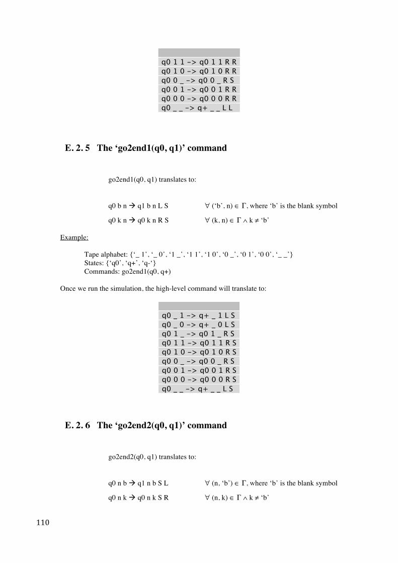
110

q0 1 1 -> q0 1 1 R R q0 1 0 -> q0 1 0 R R q0 0 _ -> q0 0 _ R S q0 0 1 -> q0 0 1 R R q0 0 0 -> q0 0 0 R R q0 _ _ -> q+ _ _ L L

E. 2. 5 The ‘go2end1(q0, q1)’ command

go2end1(q0, q1) translates to:

q0 b n q1 b n L S ∀ (‘b’, n) ∈ Γ, where ‘b’ is the blank symbol

q0 k n q0 k n R S ∀ (k, n) ∈ Γ ∧ k ≠ ‘b’ Example: Tape alphabet: {‘_ 1’, ‘_ 0’, ‘1 _’, ‘1 1’, ‘1 0’, ‘0 _’, ‘0 1’, ‘0 0’, ‘_ _’} States: {‘q0’, ‘q+’, ‘q-‘}

Commands: go2end1(q0, q+)


q0 _ 1 -> q+ _ 1 L S q0 _ 0 -> q+ _ 0 L S q0 1 _ -> q0 1 _ R S q0 1 1 -> q0 1 1 R S q0 1 0 -> q0 1 0 R S q0 0 _ -> q0 0 _ R S q0 0 1 -> q0 0 1 R S q0 0 0 -> q0 0 0 R S q0 _ _ -> q+ _ _ L S

E. 2. 6 The ‘go2end2(q0, q1)’ command

go2end2(q0, q1) translates to:

q0 n b q1 n b S L ∀ (n, ‘b’) ∈ Γ, where ‘b’ is the blank symbol

q0 n k q0 n k S R ∀ (n, k) ∈ Γ ∧ k ≠ ‘b’

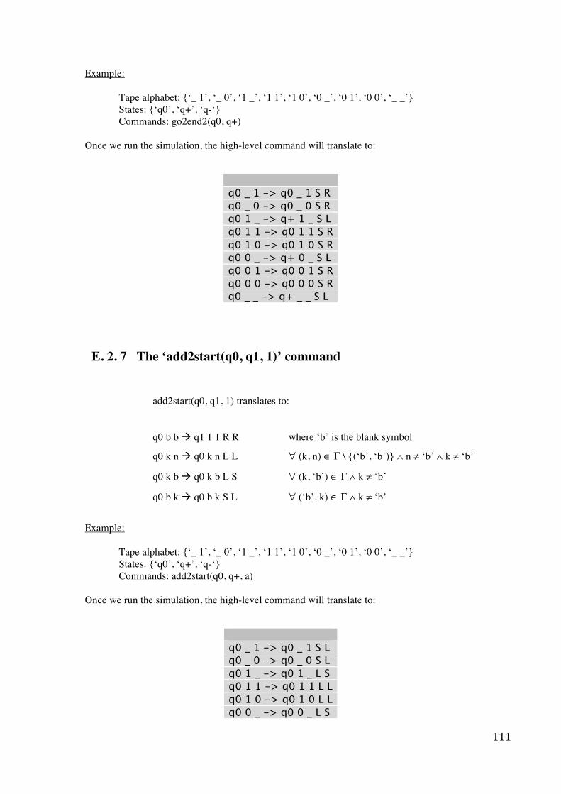
111


Commands: go2end2(q0, q+) Once we run the simulation, the high-level command will translate to:

q0 _ 1 -> q0 _ 1 S R q0 _ 0 -> q0 _ 0 S R q0 1 _ -> q+ 1 _ S L q0 1 1 -> q0 1 1 S R q0 1 0 -> q0 1 0 S R q0 0 _ -> q+ 0 _ S L q0 0 1 -> q0 0 1 S R q0 0 0 -> q0 0 0 S R q0 _ _ -> q+ _ _ S L

E. 2. 7 The ‘add2start(q0, q1, 1)’ command

add2start(q0, q1, 1) translates to:

q0 b b q1 1 1 R R where ‘b’ is the blank symbol


q0 k b q0 k b L S ∀ (k, ‘b’) ∈ Γ ∧ k ≠ ‘b’

q0 b k q0 b k S L ∀ (‘b’, k) ∈ Γ ∧ k ≠ ‘b’


Commands: add2start(q0, q+, a)


q0 _ 1 -> q0 _ 1 S L q0 _ 0 -> q0 _ 0 S L q0 1 _ -> q0 1 _ L S q0 1 1 -> q0 1 1 L L q0 1 0 -> q0 1 0 L L q0 0 _ -> q0 0 _ L S

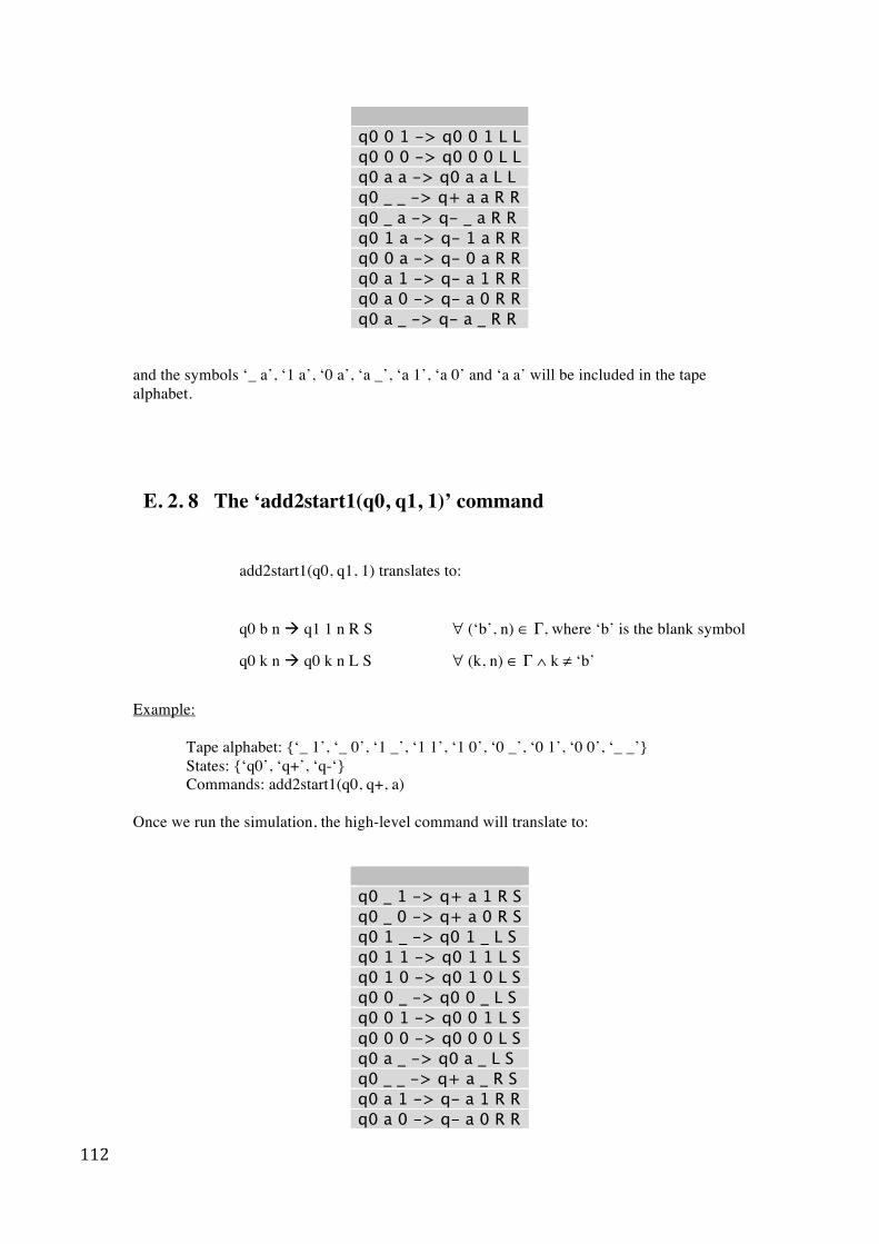
112

q0 0 1 -> q0 0 1 L L q0 0 0 -> q0 0 0 L L q0 a a -> q0 a a L L q0 _ _ -> q+ a a R R q0 _ a -> q- _ a R R q0 1 a -> q- 1 a R R q0 0 a -> q- 0 a R R q0 a 1 -> q- a 1 R R q0 a 0 -> q- a 0 R R q0 a _ -> q- a _ R R

and the symbols ‘_ a’, ‘1 a’, ‘0 a’, ‘a _’, ‘a 1’, ‘a 0’ and ‘a a’ will be included in the tape alphabet.

E. 2. 8 The ‘add2start1(q0, q1, 1)’ command

add2start1(q0, q1, 1) translates to:

q0 b n q1 1 n R S ∀ (‘b’, n) ∈ Γ, where ‘b’ is the blank symbol

q0 k n q0 k n L S ∀ (k, n) ∈ Γ ∧ k ≠ ‘b’


Commands: add2start1(q0, q+, a)


q0 _ 1 -> q+ a 1 R S q0 _ 0 -> q+ a 0 R S q0 1 _ -> q0 1 _ L S q0 1 1 -> q0 1 1 L S q0 1 0 -> q0 1 0 L S q0 0 _ -> q0 0 _ L S q0 0 1 -> q0 0 1 L S q0 0 0 -> q0 0 0 L S q0 a _ -> q0 a _ L S q0 _ _ -> q+ a _ R S q0 a 1 -> q- a 1 R R q0 a 0 -> q- a 0 R R

113

and the symbols ‘a _’, ‘a 1’ and ‘a 0’ will be included in the tape alphabet.

E. 2. 9 The ‘add2start2(q0, q1, 1)’ command

add2start2(q0, q1, 1) translates to:

q0 n b q1 n 1 S R ∀ (n, ‘b’) ∈ Γ, where ‘b’ is the blank symbol

q0 n k q0 n k S L ∀ (n, k) ∈ Γ ∧ k ≠ ‘b’


Commands: add2start2(q0, q+, a)


q0 _ 1 -> q0 _ 1 S L q0 _ 0 -> q0 _ 0 S L q0 1 _ -> q+ 1 a S R q0 1 1 -> q0 1 1 S L q0 1 0 -> q0 1 0 S L q0 0 _ -> q+ 0 a S R q0 0 1 -> q0 0 1 S L q0 0 0 -> q0 0 0 S L q0 _ a -> q0 _ a S L q0 _ _ -> q+ _ a S R q0 1 a -> q- 1 a R R q0 0 a -> q- 0 a R R

and the symbols ‘_ a’, ‘1 a’ and ‘0 a’ will be included in the tape alphabet.

E. 2. 10 The ‘add2end(q0, q1, 1)’ command

add2end(q0, q1, 1) translates to:

q0 b b q1 1 1 L L where ‘b’ is the blank symbol

114

q0 k n q0 k n R R ∀ (k, n) ∈ Γ \ {(‘b’, ‘b’)} ∧ n ≠ ‘b’ ∧ k ≠ ‘b’

q0 k b q0 k b R S ∀ (k, ‘b’) ∈ Γ ∧ k ≠ ‘b’

q0 b k q0 b k S R ∀ (‘b’, k) ∈ Γ ∧ k ≠ ‘b’


Commands: add2end(q0, q+, a)


q0 _ 1 -> q0 _ 1 S R q0 _ 0 -> q0 _ 0 S R q0 1 _ -> q0 1 _ R S q0 1 1 -> q0 1 1 R R q0 1 0 -> q0 1 0 R R q0 0 _ -> q0 0 _ R S q0 0 1 -> q0 0 1 R R q0 0 0 -> q0 0 0 R R q0 a a -> q0 a a R R q0 _ _ -> q+ a a L L q0 _ a -> q- _ a R R q0 1 a -> q- 1 a R R q0 0 a -> q- 0 a R R q0 a 1 -> q- a 1 R R q0 a 0 -> q- a 0 R R q0 a _ -> q- a _ R R

and the symbols ‘_ a’, ‘1 a’, ‘0 a’, ‘a _’, ‘a 1’, ‘a 0’ and ‘a a’ will be included in the tape alphabet.

E. 2. 11 The ‘add2end1(q0, q1, 1)’ command

add2end1(q0, q1, 1) translates to:

q0 b n q1 1 n L S ∀ (‘b’, n) ∈ Γ, where ‘b’ is the blank symbol

q0 k n q0 k n R S ∀ (k, n) ∈ Γ ∧ k ≠ ‘b’

115


Commands: add2end1(q0, q+, a)


q0 _ 1 -> q+ a 1 L S q0 _ 0 -> q+ a 0 L S q0 0 _ -> q0 0 _ R S q0 0 0 -> q0 0 0 R S q0 0 1 -> q0 0 1 R S q0 1 _ -> q0 1 _ R S q0 1 0 -> q0 1 0 R S q0 1 1 -> q0 1 1 R S q0 a 0 -> q0 a 0 R S q0 a 1 -> q0 a 1 R S q0 a _ -> q0 a _ R S q0 _ _ -> q+ a _ L S

and the symbols ‘a _’, ‘a 1’ and ‘a 0’ will be included in the tape alphabet.

E. 2. 12 The ‘add2end2(q0, q1, 1)’ command

add2end2(q0, q1, 1) translates to:

q0 n b q1 n 1 S L ∀ (n, ‘b’) ∈ Γ, where ‘b’ is the blank symbol

q0 n k q0 n k S R ∀ (n, k) ∈ Γ ∧ k ≠ ‘b’


Commands: add2end2(q0, q+, a)


116

q0 _ 0 -> q0 _ 0 S R q0 _ 1 -> q0 _ 1 S R q0 0 _ -> q+ 0 a S L q0 0 0 -> q0 0 0 S R q0 0 1 -> q0 0 1 S R q0 1 _ -> q+ 1 a S L q0 1 0 -> q0 1 0 S R q0 1 1 -> q0 1 1 S R q0 _ a -> q0 _ a S R q0 0 a -> q0 0 a S R q0 1 a -> q0 1 a S R q0 _ _ -> q+ _ a S L

and the symbols ‘_ a’, ‘1 a’ and ‘0 a’ will be included in the tape alphabet.

E. 2. 13 The ‘find(q0, q1, q2, 1, 2, D)’ command

find(q0, q1, q2, 1, 2, D) translates to:

q0 b b q2 b b D’ D’ where ‘b’ is the blank symbol and D ≠ D’

q0 k b q2 k b S D’ ∀ (k, ‘b’) ∈ Γ ∧ k ≠ ‘b’ and D ≠ D’

q0 b k q2 b k D’ S ∀ (‘b’, k) ∈ Γ ∧ k ≠ ‘b’ and D ≠ D’

q0 k n q0 k n D D ∀ (k, n) ∈ Γ \ {(‘1’,’2’), (‘b’,’b’)}

q0 1 2 q1 1 2 D D


Commands: find(q0, q+, q-, 1, 0, R)


q0 _ 0 -> q- _ 0 L S q0 _ 1 -> q- _ 1 L S q0 0 _ -> q- 0 _ S L q0 0 0 -> q0 0 0 R R q0 0 1 -> q0 0 1 R R

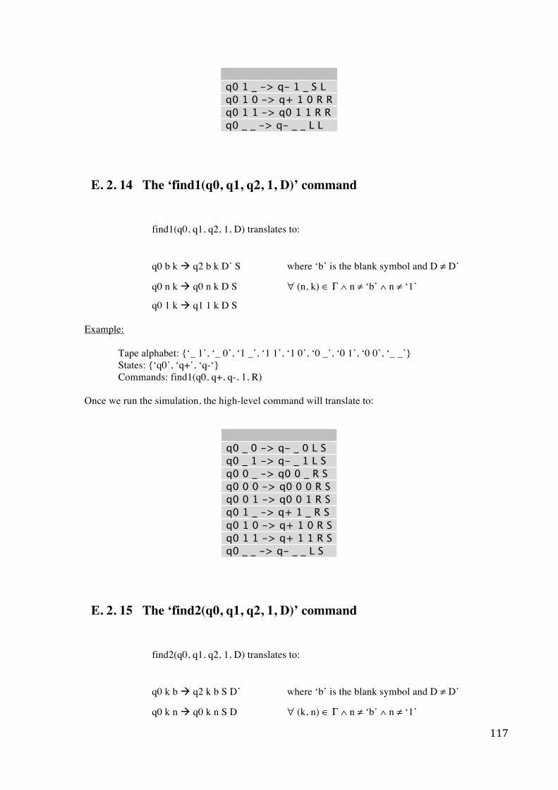
117

q0 1 _ -> q- 1 _ S L q0 1 0 -> q+ 1 0 R R q0 1 1 -> q0 1 1 R R q0 _ _ -> q- _ _ L L

E. 2. 14 The ‘find1(q0, q1, q2, 1, D)’ command

find1(q0, q1, q2, 1, D) translates to:

q0 b k q2 b k D’ S where ‘b’ is the blank symbol and D ≠ D’

q0 n k q0 n k D S ∀ (n, k) ∈ Γ ∧ n ≠ ‘b’ ∧ n ≠ ‘1’

q0 1 k q1 1 k D S Example: Tape alphabet: {‘_ 1’, ‘_ 0’, ‘1 _’, ‘1 1’, ‘1 0’, ‘0 _’, ‘0 1’, ‘0 0’, ‘_ _’} States: {‘q0’, ‘q+’, ‘q-‘}

Commands: find1(q0, q+, q-, 1, R)


q0 _ 0 -> q- _ 0 L S q0 _ 1 -> q- _ 1 L S q0 0 _ -> q0 0 _ R S q0 0 0 -> q0 0 0 R S q0 0 1 -> q0 0 1 R S q0 1 _ -> q+ 1 _ R S q0 1 0 -> q+ 1 0 R S q0 1 1 -> q+ 1 1 R S q0 _ _ -> q- _ _ L S

E. 2. 15 The ‘find2(q0, q1, q2, 1, D)’ command

find2(q0, q1, q2, 1, D) translates to:

q0 k b q2 k b S D’ where ‘b’ is the blank symbol and D ≠ D’

q0 k n q0 k n S D ∀ (k, n) ∈ Γ ∧ n ≠ ‘b’ ∧ n ≠ ‘1’

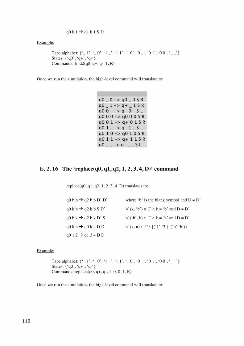
118

q0 k 1 q1 k 1 S D


Commands: find2(q0, q+, q-, 1, R)


q0 _ 0 -> q0 _ 0 S R q0 _ 1 -> q+ _ 1 S R q0 0 _ -> q- 0 _ S L q0 0 0 -> q0 0 0 S R q0 0 1 -> q+ 0 1 S R q0 1 _ -> q- 1 _ S L q0 1 0 -> q0 1 0 S R q0 1 1 -> q+ 1 1 S R q0 _ _ -> q- _ _ S L

E. 2. 16 The ‘replace(q0, q1, q2, 1, 2, 3, 4, D)’ command

replace(q0, q1, q2, 1, 2, 3, 4, D) translates to:

q0 b b q2 b b D’ D’ where ‘b’ is the blank symbol and D ≠ D’

q0 k b q2 k b S D’ ∀ (k, ‘b’) ∈ Γ ∧ k ≠ ‘b’ and D ≠ D’

q0 b k q2 b k D’ S ∀ (‘b’, k) ∈ Γ ∧ k ≠ ‘b’ and D ≠ D’

q0 k n q0 k n D D ∀ (k, n) ∈ Γ \ {(‘1’,’2’), (‘b’,’b’)}

q0 1 2 q1 3 4 D D


Commands: replace(q0, q+, q-, 1, 0, 0, 1, R)


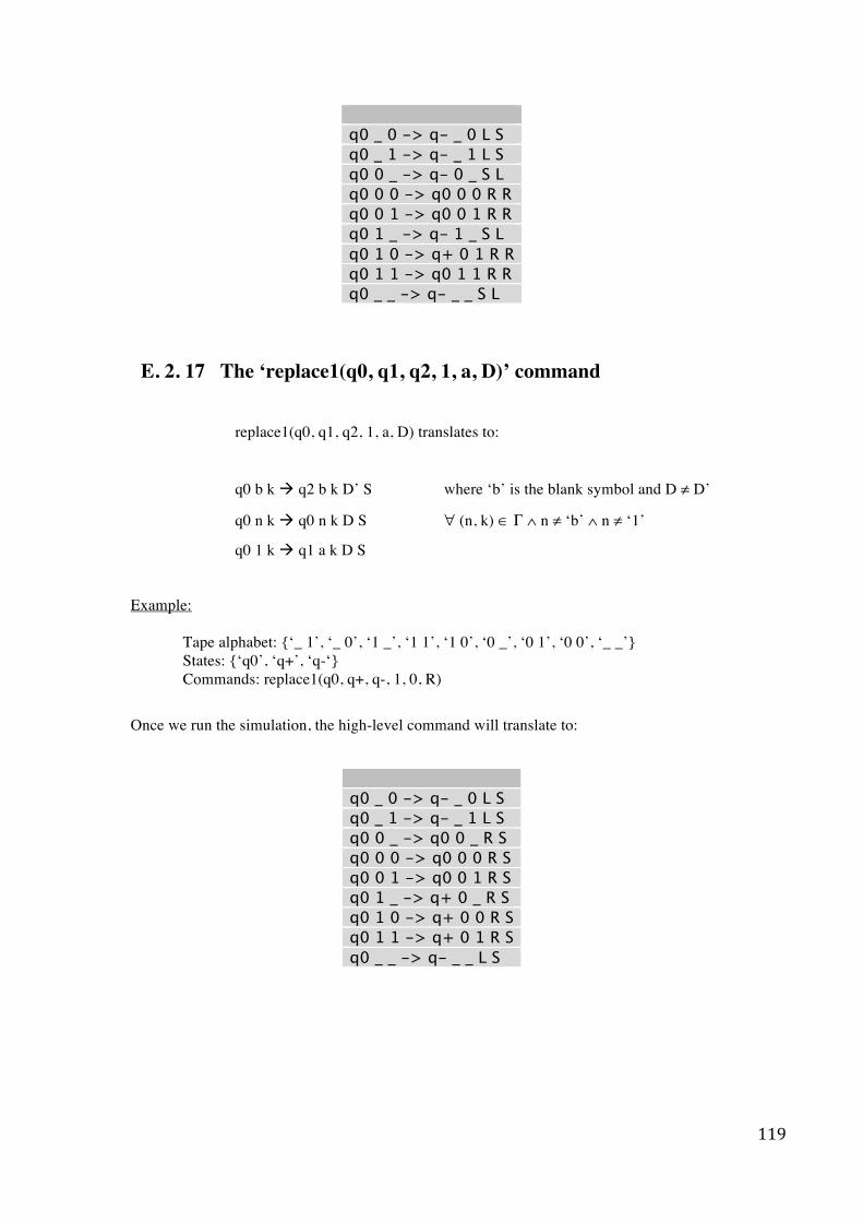
119

q0 _ 0 -> q- _ 0 L S q0 _ 1 -> q- _ 1 L S q0 0 _ -> q- 0 _ S L q0 0 0 -> q0 0 0 R R q0 0 1 -> q0 0 1 R R q0 1 _ -> q- 1 _ S L q0 1 0 -> q+ 0 1 R R q0 1 1 -> q0 1 1 R R q0 _ _ -> q- _ _ S L

E. 2. 17 The ‘replace1(q0, q1, q2, 1, a, D)’ command

replace1(q0, q1, q2, 1, a, D) translates to:

q0 b k q2 b k D’ S where ‘b’ is the blank symbol and D ≠ D’

q0 n k q0 n k D S ∀ (n, k) ∈ Γ ∧ n ≠ ‘b’ ∧ n ≠ ‘1’

q0 1 k q1 a k D S


Commands: replace1(q0, q+, q-, 1, 0, R)


q0 _ 0 -> q- _ 0 L S q0 _ 1 -> q- _ 1 L S q0 0 _ -> q0 0 _ R S q0 0 0 -> q0 0 0 R S q0 0 1 -> q0 0 1 R S q0 1 _ -> q+ 0 _ R S q0 1 0 -> q+ 0 0 R S q0 1 1 -> q+ 0 1 R S q0 _ _ -> q- _ _ L S

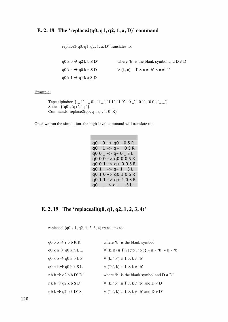
120

E. 2. 18 The ‘replace2(q0, q1, q2, 1, a, D)’ command

replace2(q0, q1, q2, 1, a, D) translates to:

q0 k b q2 k b S D’ where ‘b’ is the blank symbol and D ≠ D’

q0 k n q0 k n S D ∀ (k, n) ∈ Γ ∧ n ≠ ‘b’ ∧ n ≠ ‘1’

q0 k 1 q1 k a S D


Commands: replace2(q0, q+, q-, 1, 0, R)


q0 _ 0 -> q0 _ 0 S R q0 _ 1 -> q+ _ 0 S R q0 0 _ -> q- 0 _ S L q0 0 0 -> q0 0 0 S R q0 0 1 -> q+ 0 0 S R q0 1 _ -> q- 1 _ S L q0 1 0 -> q0 1 0 S R q0 1 1 -> q+ 1 0 S R q0 _ _ -> q- _ _ S L

E. 2. 19 The ‘replaceall(q0, q1, q2, 1, 2, 3, 4)’

replaceall(q0, q1, q2, 1, 2, 3, 4) translates to:

q0 b b r b b R R where ‘b’ is the blank symbol


q0 k b q0 k b L S ∀ (k, ‘b’) ∈ Γ ∧ k ≠ ‘b’

q0 b k q0 b k S L ∀ (‘b’, k) ∈ Γ ∧ k ≠ ‘b’

r b b q2 b b D’ D’ where ‘b’ is the blank symbol and D ≠ D’

r k b q2 k b S D’ ∀ (k, ‘b’) ∈ Γ ∧ k ≠ ‘b’ and D ≠ D’

r b k q2 b k D’ S ∀ (‘b’, k) ∈ Γ ∧ k ≠ ‘b’ and D ≠ D’

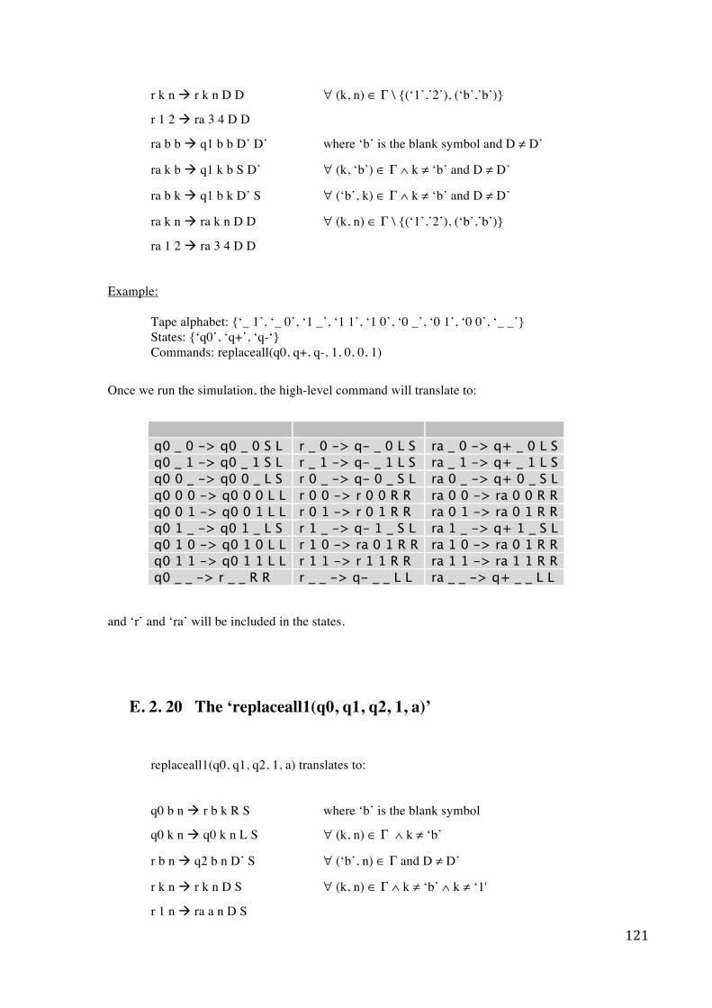
121

r k n r k n D D ∀ (k, n) ∈ Γ \ {(‘1’,’2’), (‘b’,’b’)}

r 1 2 ra 3 4 D D

ra b b q1 b b D’ D’ where ‘b’ is the blank symbol and D ≠ D’

ra k b q1 k b S D’ ∀ (k, ‘b’) ∈ Γ ∧ k ≠ ‘b’ and D ≠ D’

ra b k q1 b k D’ S ∀ (‘b’, k) ∈ Γ ∧ k ≠ ‘b’ and D ≠ D’

ra k n ra k n D D ∀ (k, n) ∈ Γ \ {(‘1’,’2’), (‘b’,’b’)}

ra 1 2 ra 3 4 D D


Commands: replaceall(q0, q+, q-, 1, 0, 0, 1)


q0 _ 0 -> q0 _ 0 S L r _ 0 -> q- _ 0 L S ra _ 0 -> q+ _ 0 L S q0 _ 1 -> q0 _ 1 S L r _ 1 -> q- _ 1 L S ra _ 1 -> q+ _ 1 L S q0 0 _ -> q0 0 _ L S r 0 _ -> q- 0 _ S L ra 0 _ -> q+ 0 _ S L q0 0 0 -> q0 0 0 L L r 0 0 -> r 0 0 R R ra 0 0 -> ra 0 0 R R q0 0 1 -> q0 0 1 L L r 0 1 -> r 0 1 R R ra 0 1 -> ra 0 1 R R q0 1 _ -> q0 1 _ L S r 1 _ -> q- 1 _ S L ra 1 _ -> q+ 1 _ S L q0 1 0 -> q0 1 0 L L r 1 0 -> ra 0 1 R R ra 1 0 -> ra 0 1 R R q0 1 1 -> q0 1 1 L L r 1 1 -> r 1 1 R R ra 1 1 -> ra 1 1 R R q0 _ _ -> r _ _ R R r _ _ -> q- _ _ L L ra _ _ -> q+ _ _ L L

and ‘r’ and ‘ra’ will be included in the states.

E. 2. 20 The ‘replaceall1(q0, q1, q2, 1, a)’

replaceall1(q0, q1, q2, 1, a) translates to:

q0 b n r b k R S where ‘b’ is the blank symbol

q0 k n q0 k n L S ∀ (k, n) ∈ Γ ∧ k ≠ ‘b’

r b n q2 b n D’ S ∀ (‘b’, n) ∈ Γ and D ≠ D’

r k n r k n D S ∀ (k, n) ∈ Γ ∧ k ≠ ‘b’ ∧ k ≠ ‘1'

r 1 n ra a n D S

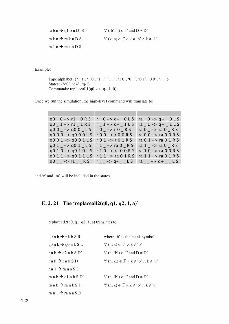
122

ra b n q1 b n D’ S ∀ (‘b’, n) ∈ Γ and D ≠ D’

ra k n ra k n D S ∀ (k, n) ∈ Γ ∧ k ≠ ‘b’ ∧ k ≠ ‘1'

ra 1 n ra a n D S


Commands: replaceall1(q0, q+, q-, 1, 0)


q0 _ 0 -> r1 _ 0 R S r _ 0 -> q- _ 0 L S ra _ 0 -> q+ _ 0 L S q0 _ 1 -> r1 _ 1 R S r _ 1 -> q- _ 1 L S ra _ 1 -> q+ _ 1 L S q0 0 _ -> q0 0 _ L S r 0 _ -> r 0 _ R S ra 0 _ -> ra 0 _ R S q0 0 0 -> q0 0 0 L S r 0 0 -> r 0 0 R S ra 0 0 -> ra 0 0 R S q0 0 1 -> q0 0 1 L S r 0 1 -> r 0 1 R S ra 0 1 -> ra 0 1 R S q0 1 _ -> q0 1 _ L S r 1 _ -> ra 0 _ R S ra 1 _ -> ra 0 _ R S q0 1 0 -> q0 1 0 L S r 1 0 -> ra 0 0 R S ra 1 0 -> ra 0 0 R S q0 1 1 -> q0 1 1 L S r 1 1 -> ra 0 1 R S ra 1 1 -> ra 0 1 R S q0 _ _ -> r1 _ _ R S r _ _ -> q- _ _ L S ra _ _ -> q+ _ _ L S


E. 2. 21 The ‘replaceall2(q0, q1, q2, 1, a)’

replaceall2(q0, q1, q2, 1, a) translates to:

q0 n b r k b S R where ‘b’ is the blank symbol

q0 n k q0 n k S L ∀ (n, k) ∈ Γ ∧ k ≠ ‘b’

r n b q2 n b S D’ ∀ (n, ‘b’) ∈ Γ and D ≠ D’

r n k r n k S D ∀ (n, k,) ∈ Γ ∧ k ≠ ‘b’ ∧ k ≠ ‘1'

r n 1 ra n a S D

ra n b q1 n b S D’ ∀ (n, ‘b’) ∈ Γ and D ≠ D’

ra n k ra n k S D ∀ (n, k) ∈ Γ ∧ k ≠ ‘b’ ∧ k ≠ ‘1'

ra n 1 ra n a S D

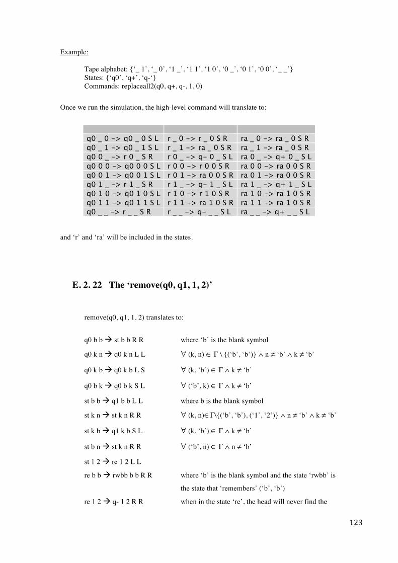
123


Commands: replaceall2(q0, q+, q-, 1, 0)


q0 _ 0 -> q0 _ 0 S L r _ 0 -> r _ 0 S R ra _ 0 -> ra _ 0 S R q0 _ 1 -> q0 _ 1 S L r _ 1 -> ra _ 0 S R ra _ 1 -> ra _ 0 S R q0 0 _ -> r 0 _ S R r 0 _ -> q- 0 _ S L ra 0 _ -> q+ 0 _ S L q0 0 0 -> q0 0 0 S L r 0 0 -> r 0 0 S R ra 0 0 -> ra 0 0 S R q0 0 1 -> q0 0 1 S L r 0 1 -> ra 0 0 S R ra 0 1 -> ra 0 0 S R q0 1 _ -> r 1 _ S R r 1 _ -> q- 1 _ S L ra 1 _ -> q+ 1 _ S L q0 1 0 -> q0 1 0 S L r 1 0 -> r 1 0 S R ra 1 0 -> ra 1 0 S R q0 1 1 -> q0 1 1 S L r 1 1 -> ra 1 0 S R ra 1 1 -> ra 1 0 S R q0 _ _ -> r _ _ S R r _ _ -> q- _ _ S L ra _ _ -> q+ _ _ S L


E. 2. 22 The ‘remove(q0, q1, 1, 2)’

remove(q0, q1, 1, 2) translates to:

q0 b b st b b R R where ‘b’ is the blank symbol


q0 k b q0 k b L S ∀ (k, ‘b’) ∈ Γ ∧ k ≠ ‘b’

q0 b k q0 b k S L ∀ (‘b’, k) ∈ Γ ∧ k ≠ ‘b’

st b b q1 b b L L where b is the blank symbol

st k n st k n R R ∀ (k, n)∈Γ\{(‘b’, ‘b’), (‘1’, ‘2’)} ∧ n ≠ ‘b’ ∧ k ≠ ‘b’

st k b q1 k b S L ∀ (k, ‘b’) ∈ Γ ∧ k ≠ ‘b’

st b n st k n R R ∀ (‘b’, n) ∈ Γ ∧ n ≠ ‘b’

st 1 2 re 1 2 L L

re b b rwbb b b R R where ‘b’ is the blank symbol and the state ‘rwbb’ is

the state that ‘remembers’ (‘b’, ‘b’)

re 1 2 q- 1 2 R R when in the state ‘re’, the head will never find the

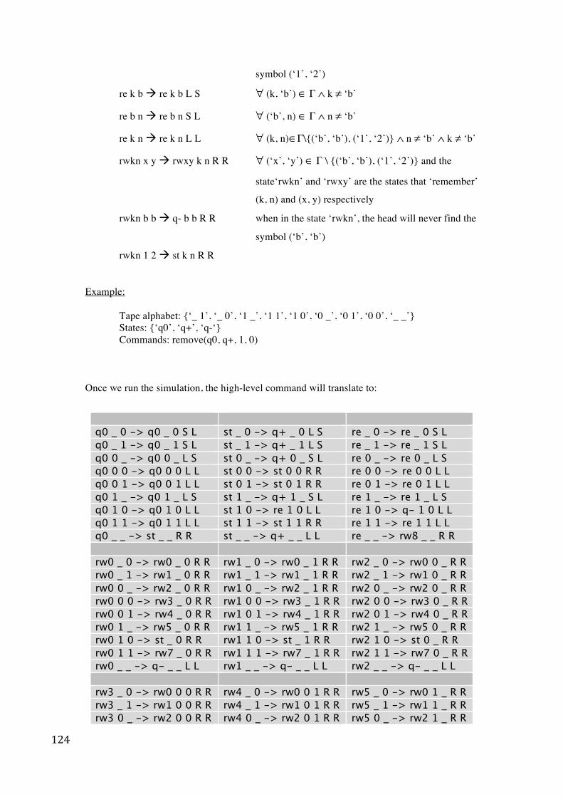
124

symbol (‘1’, ‘2’)

re k b re k b L S ∀ (k, ‘b’) ∈ Γ ∧ k ≠ ‘b’

re b n re b n S L ∀ (‘b’, n) ∈ Γ ∧ n ≠ ‘b’

re k n re k n L L ∀ (k, n)∈Γ\{(‘b’, ‘b’), (‘1’, ‘2’)} ∧ n ≠ ‘b’ ∧ k ≠ ‘b’

rwkn x y rwxy k n R R ∀ (‘x’, ‘y’) ∈ Γ \ {(‘b’, ‘b’), (‘1’, ‘2’)} and the

state‘rwkn’ and ‘rwxy’ are the states that ‘remember’

(k, n) and (x, y) respectively

rwkn b b q- b b R R when in the state ‘rwkn’, the head will never find the

symbol (‘b’, ‘b’)

rwkn 1 2 st k n R R


Commands: remove(q0, q+, 1, 0)


q0 _ 0 -> q0 _ 0 S L st _ 0 -> q+ _ 0 L S re _ 0 -> re _ 0 S L q0 _ 1 -> q0 _ 1 S L st _ 1 -> q+ _ 1 L S re _ 1 -> re _ 1 S L q0 0 _ -> q0 0 _ L S st 0 _ -> q+ 0 _ S L re 0 _ -> re 0 _ L S q0 0 0 -> q0 0 0 L L st 0 0 -> st 0 0 R R re 0 0 -> re 0 0 L L q0 0 1 -> q0 0 1 L L st 0 1 -> st 0 1 R R re 0 1 -> re 0 1 L L q0 1 _ -> q0 1 _ L S st 1 _ -> q+ 1 _ S L re 1 _ -> re 1 _ L S q0 1 0 -> q0 1 0 L L st 1 0 -> re 1 0 L L re 1 0 -> q- 1 0 L L q0 1 1 -> q0 1 1 L L st 1 1 -> st 1 1 R R re 1 1 -> re 1 1 L L q0 _ _ -> st _ _ R R st _ _ -> q+ _ _ L L re _ _ -> rw8 _ _ R R rw0 _ 0 -> rw0 _ 0 R R rw1 _ 0 -> rw0 _ 1 R R rw2 _ 0 -> rw0 0 _ R R rw0 _ 1 -> rw1 _ 0 R R rw1 _ 1 -> rw1 _ 1 R R rw2 _ 1 -> rw1 0 _ R R rw0 0 _ -> rw2 _ 0 R R rw1 0 _ -> rw2 _ 1 R R rw2 0 _ -> rw2 0 _ R R rw0 0 0 -> rw3 _ 0 R R rw1 0 0 -> rw3 _ 1 R R rw2 0 0 -> rw3 0 _ R R rw0 0 1 -> rw4 _ 0 R R rw1 0 1 -> rw4 _ 1 R R rw2 0 1 -> rw4 0 _ R R rw0 1 _ -> rw5 _ 0 R R rw1 1 _ -> rw5 _ 1 R R rw2 1 _ -> rw5 0 _ R R rw0 1 0 -> st _ 0 R R rw1 1 0 -> st _ 1 R R rw2 1 0 -> st 0 _ R R rw0 1 1 -> rw7 _ 0 R R rw1 1 1 -> rw7 _ 1 R R rw2 1 1 -> rw7 0 _ R R rw0 _ _ -> q- _ _ L L rw1 _ _ -> q- _ _ L L rw2 _ _ -> q- _ _ L L rw3 _ 0 -> rw0 0 0 R R rw4 _ 0 -> rw0 0 1 R R rw5 _ 0 -> rw0 1 _ R R rw3 _ 1 -> rw1 0 0 R R rw4 _ 1 -> rw1 0 1 R R rw5 _ 1 -> rw1 1 _ R R rw3 0 _ -> rw2 0 0 R R rw4 0 _ -> rw2 0 1 R R rw5 0 _ -> rw2 1 _ R R

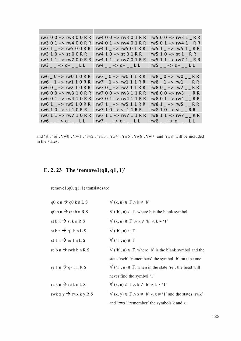
125

rw3 0 0 -> rw3 0 0 R R rw4 0 0 -> rw3 0 1 R R rw5 0 0 -> rw3 1 _ R R rw3 0 1 -> rw4 0 0 R R rw4 0 1 -> rw4 0 1 R R rw5 0 1 -> rw4 1 _ R R rw3 1 _ -> rw5 0 0 R R rw4 1 _ -> rw5 0 1 R R rw5 1 _ -> rw5 1 _ R R rw3 1 0 -> st 0 0 R R rw4 1 0 -> st 0 1 R R rw5 1 0 -> st 1 _ R R rw3 1 1 -> rw7 0 0 R R rw4 1 1 -> rw7 0 1 R R rw5 1 1 -> rw7 1 _ R R rw3 _ _ -> q- _ _ L L rw4 _ _ -> q- _ _ L L rw5 _ _ -> q- _ _ L L rw6 _ 0 -> rw0 1 0 R R rw7 _ 0 -> rw0 1 1 R R rw8 _ 0 -> rw0 _ _ R R rw6 _ 1 -> rw1 1 0 R R rw7 _ 1 -> rw1 1 1 R R rw8 _ 1 -> rw1 _ _ R R rw6 0 _ -> rw2 1 0 R R rw7 0 _ -> rw2 1 1 R R rw8 0 _ -> rw2 _ _ R R rw6 0 0 -> rw3 1 0 R R rw7 0 0 -> rw3 1 1 R R rw8 0 0 -> rw3 _ _ R R rw6 0 1 -> rw4 1 0 R R rw7 0 1 -> rw4 1 1 R R rw8 0 1 -> rw4 _ _ R R rw6 1 _ -> rw5 1 0 R R rw7 1 _ -> rw5 1 1 R R rw8 1 _ -> rw5 _ _ R R rw6 1 0 -> st 1 0 R R rw7 1 0 -> st 1 1 R R rw8 1 0 -> st _ _ R R rw6 1 1 -> rw7 1 0 R R rw7 1 1 -> rw7 1 1 R R rw8 1 1 -> rw7 _ _ R R rw6 _ _ -> q- _ _ L L rw7 _ _ -> q- _ _ L L rw8 _ _ -> q- _ _ L L

and ‘st’, ‘re’, ‘rw0’, ‘rw1’, ‘rw2’, ‘rw3’, ‘rw4’, ‘rw5’, ‘rw6’, ‘rw7’ and ‘rw8’ will be included in the states.

E. 2. 23 The ‘remove1(q0, q1, 1)’

remove1(q0, q1, 1) translates to:

q0 k n q0 k n L S ∀ (k, n) ∈ Γ ∧ k ≠ ‘b’

q0 b n q0 b n R S ∀ (‘b’, n) ∈ Γ, where b is the blank symbol

st k n st k n R S ∀ (k, n) ∈ Γ ∧ k ≠ ‘b’ ∧ k ≠ ‘1’

st b n q1 b n L S ∀ (‘b’, n) ∈ Γ

st 1 n re 1 n L S ∀ (‘1’, n) ∈ Γ

re b n rwb b n R S ∀ (‘b’, n) ∈ Γ, where ‘b’ is the blank symbol and the

state ‘rwb’ ‘remembers’ the symbol ‘b’ on tape one

re 1 n q- 1 n R S ∀ (‘1’, n) ∈ Γ, when in the state ‘re’, the head will

never find the symbol ‘1’

re k n re k n L S ∀ (k, n) ∈ Γ ∧ k ≠ ‘b’ ∧ k ≠ ‘1’

rwk x y rwx k y R S ∀ (x, y) ∈ Γ ∧ x ≠ ‘b’ ∧ x ≠ ‘1’ and the states ‘rwk’

and ‘rwx’ ‘remember’ the symbols k and x

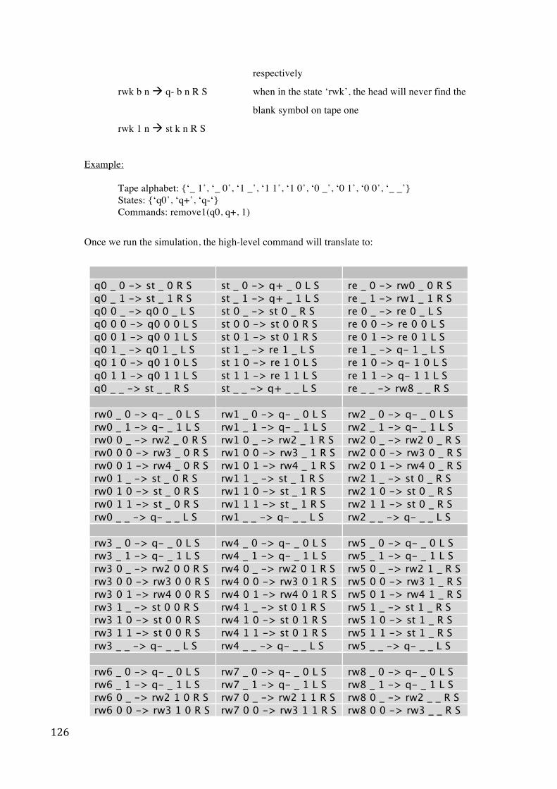
126

respectively

rwk b n q- b n R S when in the state ‘rwk’, the head will never find the

blank symbol on tape one

rwk 1 n st k n R S


Commands: remove1(q0, q+, 1)


q0 _ 0 -> st _ 0 R S st _ 0 -> q+ _ 0 L S re _ 0 -> rw0 _ 0 R S q0 _ 1 -> st _ 1 R S st _ 1 -> q+ _ 1 L S re _ 1 -> rw1 _ 1 R S q0 0 _ -> q0 0 _ L S st 0 _ -> st 0 _ R S re 0 _ -> re 0 _ L S q0 0 0 -> q0 0 0 L S st 0 0 -> st 0 0 R S re 0 0 -> re 0 0 L S q0 0 1 -> q0 0 1 L S st 0 1 -> st 0 1 R S re 0 1 -> re 0 1 L S q0 1 _ -> q0 1 _ L S st 1 _ -> re 1 _ L S re 1 _ -> q- 1 _ L S q0 1 0 -> q0 1 0 L S st 1 0 -> re 1 0 L S re 1 0 -> q- 1 0 L S q0 1 1 -> q0 1 1 L S st 1 1 -> re 1 1 L S re 1 1 -> q- 1 1 L S q0 _ _ -> st _ _ R S st _ _ -> q+ _ _ L S re _ _ -> rw8 _ _ R S rw0 _ 0 -> q- _ 0 L S rw1 _ 0 -> q- _ 0 L S rw2 _ 0 -> q- _ 0 L S rw0 _ 1 -> q- _ 1 L S rw1 _ 1 -> q- _ 1 L S rw2 _ 1 -> q- _ 1 L S rw0 0 _ -> rw2 _ 0 R S rw1 0 _ -> rw2 _ 1 R S rw2 0 _ -> rw2 0 _ R S rw0 0 0 -> rw3 _ 0 R S rw1 0 0 -> rw3 _ 1 R S rw2 0 0 -> rw3 0 _ R S rw0 0 1 -> rw4 _ 0 R S rw1 0 1 -> rw4 _ 1 R S rw2 0 1 -> rw4 0 _ R S rw0 1 _ -> st _ 0 R S rw1 1 _ -> st _ 1 R S rw2 1 _ -> st 0 _ R S rw0 1 0 -> st _ 0 R S rw1 1 0 -> st _ 1 R S rw2 1 0 -> st 0 _ R S rw0 1 1 -> st _ 0 R S rw1 1 1 -> st _ 1 R S rw2 1 1 -> st 0 _ R S rw0 _ _ -> q- _ _ L S rw1 _ _ -> q- _ _ L S rw2 _ _ -> q- _ _ L S rw3 _ 0 -> q- _ 0 L S rw4 _ 0 -> q- _ 0 L S rw5 _ 0 -> q- _ 0 L S rw3 _ 1 -> q- _ 1 L S rw4 _ 1 -> q- _ 1 L S rw5 _ 1 -> q- _ 1 L S rw3 0 _ -> rw2 0 0 R S rw4 0 _ -> rw2 0 1 R S rw5 0 _ -> rw2 1 _ R S rw3 0 0 -> rw3 0 0 R S rw4 0 0 -> rw3 0 1 R S rw5 0 0 -> rw3 1 _ R S rw3 0 1 -> rw4 0 0 R S rw4 0 1 -> rw4 0 1 R S rw5 0 1 -> rw4 1 _ R S rw3 1 _ -> st 0 0 R S rw4 1 _ -> st 0 1 R S rw5 1 _ -> st 1 _ R S rw3 1 0 -> st 0 0 R S rw4 1 0 -> st 0 1 R S rw5 1 0 -> st 1 _ R S rw3 1 1 -> st 0 0 R S rw4 1 1 -> st 0 1 R S rw5 1 1 -> st 1 _ R S rw3 _ _ -> q- _ _ L S rw4 _ _ -> q- _ _ L S rw5 _ _ -> q- _ _ L S rw6 _ 0 -> q- _ 0 L S rw7 _ 0 -> q- _ 0 L S rw8 _ 0 -> q- _ 0 L S rw6 _ 1 -> q- _ 1 L S rw7 _ 1 -> q- _ 1 L S rw8 _ 1 -> q- _ 1 L S rw6 0 _ -> rw2 1 0 R S rw7 0 _ -> rw2 1 1 R S rw8 0 _ -> rw2 _ _ R S rw6 0 0 -> rw3 1 0 R S rw7 0 0 -> rw3 1 1 R S rw8 0 0 -> rw3 _ _ R S

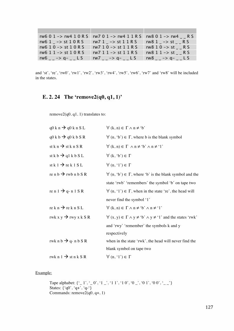
127

rw6 0 1 -> rw4 1 0 R S rw7 0 1 -> rw4 1 1 R S rw8 0 1 -> rw4 _ _ R S rw6 1 _ -> st 1 0 R S rw7 1 _ -> st 1 1 R S rw8 1 _ -> st _ _ R S rw6 1 0 -> st 1 0 R S rw7 1 0 -> st 1 1 R S rw8 1 0 -> st _ _ R S rw6 1 1 -> st 1 0 R S rw7 1 1 -> st 1 1 R S rw8 1 1 -> st _ _ R S rw6 _ _ -> q- _ _ L S rw7 _ _ -> q- _ _ L S rw8 _ _ -> q- _ _ L S

and ‘st’, ‘re’, ‘rw0’, ‘rw1’, ‘rw2’, ‘rw3’, ‘rw4’, ‘rw5’, ‘rw6’, ‘rw7’ and ‘rw8’ will be included in the states.

E. 2. 24 The ‘remove2(q0, q1, 1)’

remove2(q0, q1, 1) translates to:

q0 k n q0 k n S L ∀ (k, n) ∈ Γ ∧ n ≠ ‘b’

q0 k b q0 k b S R ∀ (n, ‘b’) ∈ Γ, where b is the blank symbol

st k n st k n S R ∀ (k, n) ∈ Γ ∧ n ≠ ‘b’ ∧ n ≠ ‘1’

st k b q1 k b S L ∀ (k, ‘b’) ∈ Γ

st k 1 re k 1 S L ∀ (n, ‘1’) ∈ Γ

re n b rwb n b S R ∀ (n, ‘b’) ∈ Γ, where ‘b’ is the blank symbol and the

state ‘rwb’ ‘remembers’ the symbol ‘b’ on tape two

re n 1 q- n 1 S R ∀ (n, ‘1’) ∈ Γ, when in the state ‘re’, the head will

never find the symbol ‘1’

re k n re k n S L ∀ (k, n) ∈ Γ ∧ n ≠ ‘b’ ∧ n ≠ ‘1’

rwk x y rwy x k S R ∀ (x, y) ∈ Γ ∧ y ≠ ‘b’ ∧ y ≠ ‘1’ and the states ‘rwk’

and ‘rwy’ ‘remember’ the symbols k and y

respectively

rwk n b q- n b S R when in the state ‘rwk’, the head will never find the

blank symbol on tape two

rwk n 1 st n k S R ∀ (n, ‘1’) ∈ Γ


Commands: remove2(q0, q+, 1)

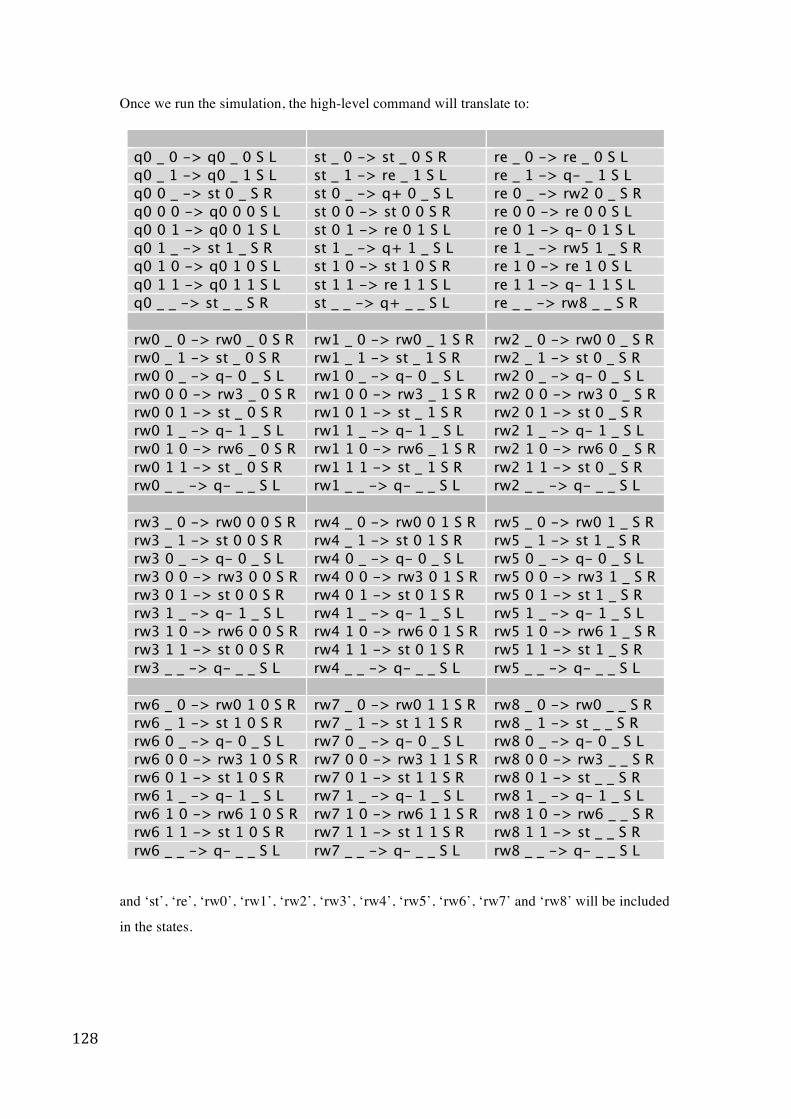
128

Once we run the simulation, the high-level command will translate to: q0 _ 0 -> q0 _ 0 S L st _ 0 -> st _ 0 S R re _ 0 -> re _ 0 S L q0 _ 1 -> q0 _ 1 S L st _ 1 -> re _ 1 S L re _ 1 -> q- _ 1 S L q0 0 _ -> st 0 _ S R st 0 _ -> q+ 0 _ S L re 0 _ -> rw2 0 _ S R q0 0 0 -> q0 0 0 S L st 0 0 -> st 0 0 S R re 0 0 -> re 0 0 S L q0 0 1 -> q0 0 1 S L st 0 1 -> re 0 1 S L re 0 1 -> q- 0 1 S L q0 1 _ -> st 1 _ S R st 1 _ -> q+ 1 _ S L re 1 _ -> rw5 1 _ S R q0 1 0 -> q0 1 0 S L st 1 0 -> st 1 0 S R re 1 0 -> re 1 0 S L q0 1 1 -> q0 1 1 S L st 1 1 -> re 1 1 S L re 1 1 -> q- 1 1 S L q0 _ _ -> st _ _ S R st _ _ -> q+ _ _ S L re _ _ -> rw8 _ _ S R rw0 _ 0 -> rw0 _ 0 S R rw1 _ 0 -> rw0 _ 1 S R rw2 _ 0 -> rw0 0 _ S R rw0 _ 1 -> st _ 0 S R rw1 _ 1 -> st _ 1 S R rw2 _ 1 -> st 0 _ S R rw0 0 _ -> q- 0 _ S L rw1 0 _ -> q- 0 _ S L rw2 0 _ -> q- 0 _ S L rw0 0 0 -> rw3 _ 0 S R rw1 0 0 -> rw3 _ 1 S R rw2 0 0 -> rw3 0 _ S R rw0 0 1 -> st _ 0 S R rw1 0 1 -> st _ 1 S R rw2 0 1 -> st 0 _ S R rw0 1 _ -> q- 1 _ S L rw1 1 _ -> q- 1 _ S L rw2 1 _ -> q- 1 _ S L rw0 1 0 -> rw6 _ 0 S R rw1 1 0 -> rw6 _ 1 S R rw2 1 0 -> rw6 0 _ S R rw0 1 1 -> st _ 0 S R rw1 1 1 -> st _ 1 S R rw2 1 1 -> st 0 _ S R rw0 _ _ -> q- _ _ S L rw1 _ _ -> q- _ _ S L rw2 _ _ -> q- _ _ S L rw3 _ 0 -> rw0 0 0 S R rw4 _ 0 -> rw0 0 1 S R rw5 _ 0 -> rw0 1 _ S R rw3 _ 1 -> st 0 0 S R rw4 _ 1 -> st 0 1 S R rw5 _ 1 -> st 1 _ S R rw3 0 _ -> q- 0 _ S L rw4 0 _ -> q- 0 _ S L rw5 0 _ -> q- 0 _ S L rw3 0 0 -> rw3 0 0 S R rw4 0 0 -> rw3 0 1 S R rw5 0 0 -> rw3 1 _ S R rw3 0 1 -> st 0 0 S R rw4 0 1 -> st 0 1 S R rw5 0 1 -> st 1 _ S R rw3 1 _ -> q- 1 _ S L rw4 1 _ -> q- 1 _ S L rw5 1 _ -> q- 1 _ S L rw3 1 0 -> rw6 0 0 S R rw4 1 0 -> rw6 0 1 S R rw5 1 0 -> rw6 1 _ S R rw3 1 1 -> st 0 0 S R rw4 1 1 -> st 0 1 S R rw5 1 1 -> st 1 _ S R rw3 _ _ -> q- _ _ S L rw4 _ _ -> q- _ _ S L rw5 _ _ -> q- _ _ S L rw6 _ 0 -> rw0 1 0 S R rw7 _ 0 -> rw0 1 1 S R rw8 _ 0 -> rw0 _ _ S R rw6 _ 1 -> st 1 0 S R rw7 _ 1 -> st 1 1 S R rw8 _ 1 -> st _ _ S R rw6 0 _ -> q- 0 _ S L rw7 0 _ -> q- 0 _ S L rw8 0 _ -> q- 0 _ S L rw6 0 0 -> rw3 1 0 S R rw7 0 0 -> rw3 1 1 S R rw8 0 0 -> rw3 _ _ S R rw6 0 1 -> st 1 0 S R rw7 0 1 -> st 1 1 S R rw8 0 1 -> st _ _ S R rw6 1 _ -> q- 1 _ S L rw7 1 _ -> q- 1 _ S L rw8 1 _ -> q- 1 _ S L rw6 1 0 -> rw6 1 0 S R rw7 1 0 -> rw6 1 1 S R rw8 1 0 -> rw6 _ _ S R rw6 1 1 -> st 1 0 S R rw7 1 1 -> st 1 1 S R rw8 1 1 -> st _ _ S R rw6 _ _ -> q- _ _ S L rw7 _ _ -> q- _ _ S L rw8 _ _ -> q- _ _ S L

and ‘st’, ‘re’, ‘rw0’, ‘rw1’, ‘rw2’, ‘rw3’, ‘rw4’, ‘rw5’, ‘rw6’, ‘rw7’ and ‘rw8’ will be included

in the states.

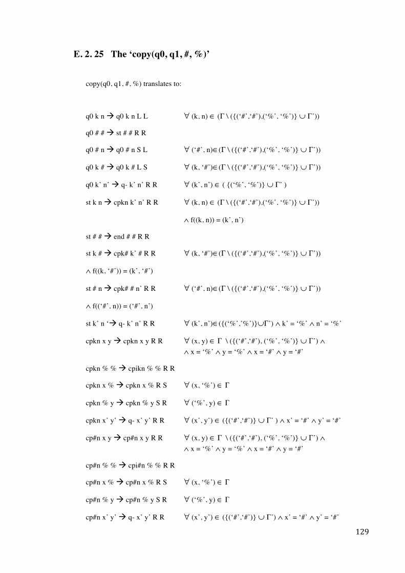
129

E. 2. 25 The ‘copy(q0, q1, #, %)’

copy(q0, q1, #, %) translates to:

q0 k n q0 k n L L ∀ (k, n) ∈ (Γ \ ({(‘#’,‘#’),(‘%’, ‘%’)} ∪ Γ’))

q0 # # st # # R R

q0 # n q0 # n S L ∀ (‘#’, n)∈(Γ \ ({(‘#’,‘#’),(‘%’, ‘%’)} ∪ Γ’))

q0 k # q0 k # L S ∀ (k, ‘#’)∈(Γ \ ({(‘#’,‘#’),(‘%’, ‘%’)} ∪ Γ’))

q0 k’ n’ q- k’ n’ R R ∀ (k’, n’) ∈ ( {(‘%’, ‘%’)} ∪ Γ’ )

st k n cpkn k’ n’ R R ∀ (k, n) ∈ (Γ \ ({(‘#’,‘#’),(‘%’, ‘%’)} ∪ Γ’))

∧ f((k, n)) = (k’, n’)

st # # end # # R R

st k # cpk# k’ # R R ∀ (k, ‘#’)∈(Γ \ ({(‘#’,‘#’),(‘%’, ‘%’)} ∪ Γ’))

∧ f((k, ‘#’)) = (k’, ‘#’)

st # n cpk# # n’ R R ∀ (‘#’, n)∈(Γ \ ({(‘#’,‘#’),(‘%’, ‘%’)} ∪ Γ’))

∧ f((‘#’, n)) = (‘#’, n’)

st k’ n ‘ q- k’ n’ R R ∀ (k’, n’)∈({(‘%’,’%’)}∪Γ’) ∧ k’ = ‘%’ ∧ n’ = ‘%’

cpkn x y cpkn x y R R ∀ (x, y) ∈ Γ \ ({(‘#’,‘#’), (‘%’, ‘%’)} ∪ Γ’) ∧ ∧ x = ‘%’ ∧ y = ‘%’ ∧ x = ‘#’ ∧ y = ‘#’

cpkn % % cpikn % % R R

cpkn x % cpkn x % R S ∀ (x, ‘%’) ∈ Γ

cpkn % y cpkn % y S R ∀ (‘%’, y) ∈ Γ

cpkn x’ y’ q- x’ y’ R R ∀ (x’, y’) ∈ ({(‘#’,‘#’)} ∪ Γ’ ) ∧ x’ = ‘#’ ∧ y’ = ‘#’

cp#n x y cp#n x y R R ∀ (x, y) ∈ Γ \ ({(‘#’,‘#’), (‘%’, ‘%’)} ∪ Γ’) ∧ ∧ x = ‘%’ ∧ y = ‘%’ ∧ x = ‘#’ ∧ y = ‘#’

cp#n % % cpi#n % % R R

cp#n x % cp#n x % R S ∀ (x, ‘%’) ∈ Γ

cp#n % y cp#n % y S R ∀ (‘%’, y) ∈ Γ

cp#n x’ y’ q- x’ y’ R R ∀ (x’, y’) ∈ ({(‘#’,‘#’)} ∪ Γ’) ∧ x’ = ‘#’ ∧ y’ = ‘#’

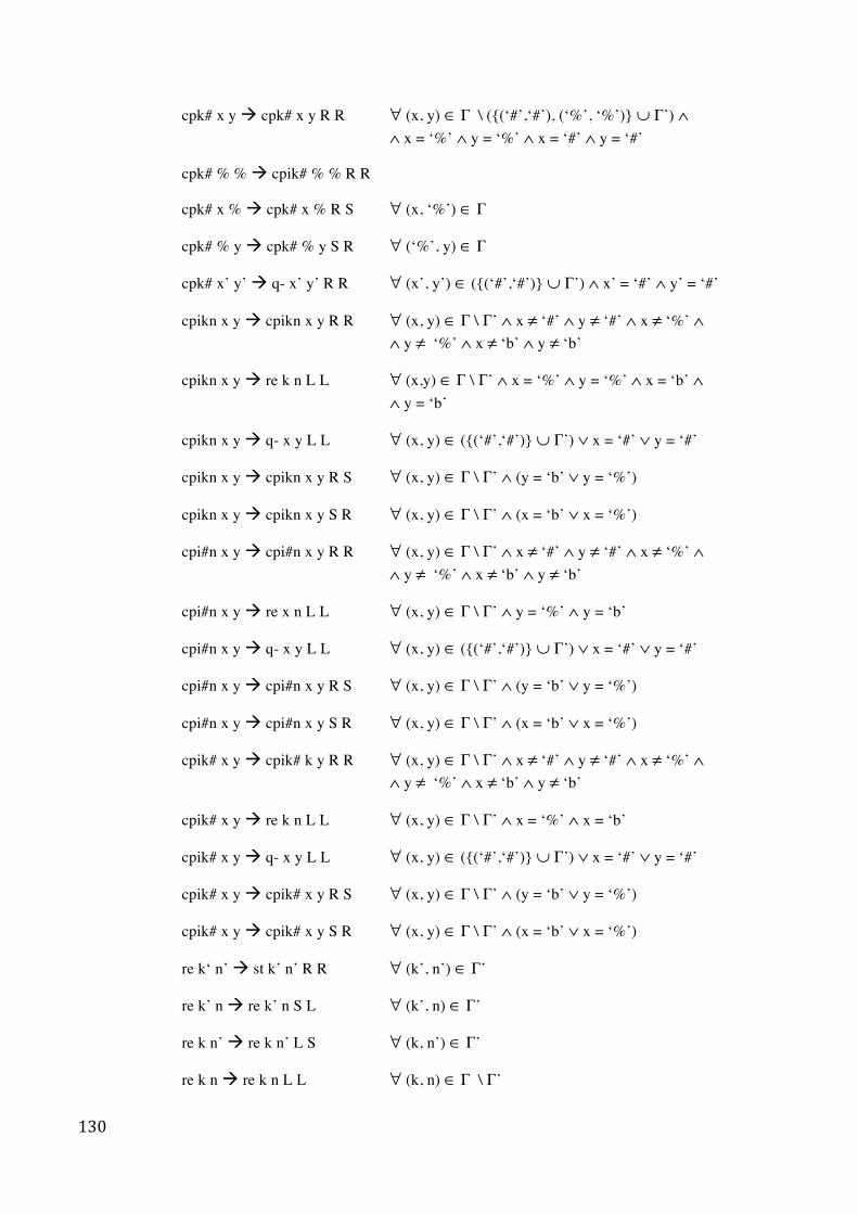
130

cpk# x y cpk# x y R R ∀ (x, y) ∈ Γ \ ({(‘#’,‘#’), (‘%’, ‘%’)} ∪ Γ’) ∧ ∧ x = ‘%’ ∧ y = ‘%’ ∧ x = ‘#’ ∧ y = ‘#’

cpk# % % cpik# % % R R

cpk# x % cpk# x % R S ∀ (x, ‘%’) ∈ Γ

cpk# % y cpk# % y S R ∀ (‘%’, y) ∈ Γ

cpk# x’ y’ q- x’ y’ R R ∀ (x’, y’) ∈ ({(‘#’,‘#’)} ∪ Γ’) ∧ x’ = ‘#’ ∧ y’ = ‘#’

cpikn x y cpikn x y R R ∀ (x, y) ∈ Γ \ Γ’ ∧ x ≠ ‘#’ ∧ y ≠ ‘#’ ∧ x ≠ ‘%’ ∧ ∧ y ≠ ‘%’ ∧ x ≠ ‘b’ ∧ y ≠ ‘b’

cpikn x y re k n L L ∀ (x,y) ∈ Γ \ Γ’ ∧ x = ‘%’ ∧ y = ‘%’ ∧ x = ‘b’ ∧ ∧ y = ‘b’

cpikn x y q- x y L L ∀ (x, y) ∈ ({(‘#’,‘#’)} ∪ Γ’) ∨ x = ‘#’ ∨ y = ‘#’

cpikn x y cpikn x y R S ∀ (x, y) ∈ Γ \ Γ’ ∧ (y = ‘b’ ∨ y = ‘%’)

cpikn x y cpikn x y S R ∀ (x, y) ∈ Γ \ Γ’ ∧ (x = ‘b’ ∨ x = ‘%’)

cpi#n x y cpi#n x y R R ∀ (x, y) ∈ Γ \ Γ’ ∧ x ≠ ‘#’ ∧ y ≠ ‘#’ ∧ x ≠ ‘%’ ∧ ∧ y ≠ ‘%’ ∧ x ≠ ‘b’ ∧ y ≠ ‘b’

cpi#n x y re x n L L ∀ (x, y) ∈ Γ \ Γ’ ∧ y = ‘%’ ∧ y = ‘b’

cpi#n x y q- x y L L ∀ (x, y) ∈ ({(‘#’,‘#’)} ∪ Γ’) ∨ x = ‘#’ ∨ y = ‘#’

cpi#n x y cpi#n x y R S ∀ (x, y) ∈ Γ \ Γ’ ∧ (y = ‘b’ ∨ y = ‘%’)

cpi#n x y cpi#n x y S R ∀ (x, y) ∈ Γ \ Γ’ ∧ (x = ‘b’ ∨ x = ‘%’)

cpik# x y cpik# k y R R ∀ (x, y) ∈ Γ \ Γ’ ∧ x ≠ ‘#’ ∧ y ≠ ‘#’ ∧ x ≠ ‘%’ ∧ ∧ y ≠ ‘%’ ∧ x ≠ ‘b’ ∧ y ≠ ‘b’

cpik# x y re k n L L ∀ (x, y) ∈ Γ \ Γ’ ∧ x = ‘%’ ∧ x = ‘b’

cpik# x y q- x y L L ∀ (x, y) ∈ ({(‘#’,‘#’)} ∪ Γ’) ∨ x = ‘#’ ∨ y = ‘#’

cpik# x y cpik# x y R S ∀ (x, y) ∈ Γ \ Γ’ ∧ (y = ‘b’ ∨ y = ‘%’)

cpik# x y cpik# x y S R ∀ (x, y) ∈ Γ \ Γ’ ∧ (x = ‘b’ ∨ x = ‘%’)

re k‘ n’ st k’ n’ R R ∀ (k’, n’) ∈ Γ’

re k’ n re k’ n S L ∀ (k’, n) ∈ Γ’

re k n’ re k n’ L S ∀ (k, n’) ∈ Γ’

re k n re k n L L ∀ (k, n) ∈ Γ \ Γ’

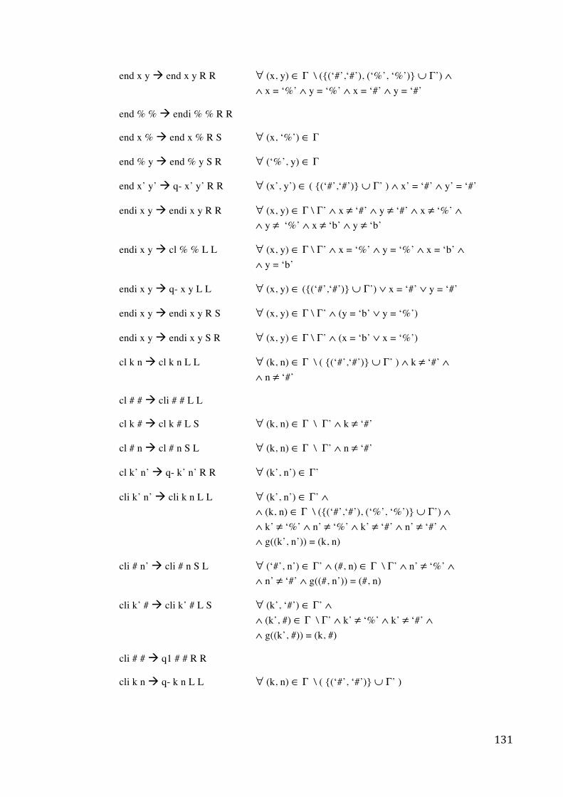
131

end x y end x y R R ∀ (x, y) ∈ Γ \ ({(‘#’,‘#’), (‘%’, ‘%’)} ∪ Γ’) ∧ ∧ x = ‘%’ ∧ y = ‘%’ ∧ x = ‘#’ ∧ y = ‘#’

end % % endi % % R R

end x % end x % R S ∀ (x, ‘%’) ∈ Γ

end % y end % y S R ∀ (‘%’, y) ∈ Γ

end x’ y’ q- x’ y’ R R ∀ (x’, y’) ∈ ( {(‘#’,‘#’)} ∪ Γ’ ) ∧ x’ = ‘#’ ∧ y’ = ‘#’

endi x y endi x y R R ∀ (x, y) ∈ Γ \ Γ’ ∧ x ≠ ‘#’ ∧ y ≠ ‘#’ ∧ x ≠ ‘%’ ∧ ∧ y ≠ ‘%’ ∧ x ≠ ‘b’ ∧ y ≠ ‘b’

endi x y cl % % L L ∀ (x, y) ∈ Γ \ Γ’ ∧ x = ‘%’ ∧ y = ‘%’ ∧ x = ‘b’ ∧ ∧ y = ‘b’

endi x y q- x y L L ∀ (x, y) ∈ ({(‘#’,‘#’)} ∪ Γ’) ∨ x = ‘#’ ∨ y = ‘#’

endi x y endi x y R S ∀ (x, y) ∈ Γ \ Γ’ ∧ (y = ‘b’ ∨ y = ‘%’)

endi x y endi x y S R ∀ (x, y) ∈ Γ \ Γ’ ∧ (x = ‘b’ ∨ x = ‘%’)

cl k n cl k n L L ∀ (k, n) ∈ Γ \ ( {(‘#’,‘#’)} ∪ Γ’ ) ∧ k ≠ ‘#’ ∧ ∧ n ≠ ‘#’

cl # # cli # # L L

cl k # cl k # L S ∀ (k, n) ∈ Γ \ Γ’ ∧ k ≠ ‘#’

cl # n cl # n S L ∀ (k, n) ∈ Γ \ Γ’ ∧ n ≠ ‘#’

cl k’ n’ q- k’ n’ R R ∀ (k’, n’) ∈ Γ’

cli k’ n’ cli k n L L ∀ (k’, n’) ∈ Γ’ ∧ ∧ (k, n) ∈ Γ \ ({(‘#’,‘#’), (‘%’, ‘%’)} ∪ Γ’) ∧ ∧ k’ ≠ ‘%’ ∧ n’ ≠ ‘%’ ∧ k’ ≠ ‘#’ ∧ n’ ≠ ‘#’ ∧ ∧ g((k’, n’)) = (k, n)

cli # n’ cli # n S L ∀ (‘#’, n’) ∈ Γ’ ∧ (#, n) ∈ Γ \ Γ’ ∧ n’ ≠ ‘%’ ∧ ∧ n’ ≠ ‘#’ ∧ g((#, n’)) = (#, n)

cli k’ # cli k’ # L S ∀ (k’, ‘#’) ∈ Γ’ ∧ ∧ (k’, #) ∈ Γ \ Γ’ ∧ k’ ≠ ‘%’ ∧ k’ ≠ ‘#’ ∧ ∧ g((k’, #)) = (k, #)

cli # # q1 # # R R

cli k n q- k n L L ∀ (k, n) ∈ Γ \ ( {(‘#’, ‘#’)} ∪ Γ’ )

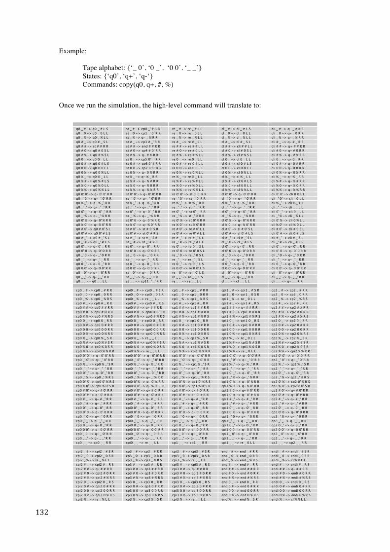
132

Example: Tape alphabet: {‘_ 0’, ‘0 _’, ‘0 0’, ‘_ _’} States: {‘q0’, ‘q+’, ‘q-‘}

Commands: copy(q0, q+, #, %)


q0 _ # -> q0 _ # L S st _ # -> cp0 _' # R R re _ # -> re _ # L L cl _ # -> cl _ # L S cli _ # -> q- _ # R R q0 _ 0 -> q0 _ 0 L L st _ 0 -> cp1 _' 0' R R re _ 0 -> re _ 0 L L cl _ 0 -> cl _ 0 L L cli _ 0 -> q- _ 0 R R q0 _ % -> q0 _ % L L st _ % -> q- _ % R R re _ % -> re _ % L L cl _ % -> cl _ % L L cli _ % -> q- _ % R R q0 # _ -> q0 # _ S L st # _ -> cp3 # _' R R re # _ -> re # _ L L cl # _ -> cl # _ S L cli # _ -> q- # _ R R q0 # # -> st # # R R st # # -> end # # R R re # # -> re # # L L cl # # -> cli # # L L cli # # -> q+ # # R R q0 # 0 -> q0 # 0 S L st # 0 -> cp4 # 0' R R re # 0 -> re # 0 L L cl # 0 -> cl # 0 S L cli # 0 -> q- # 0 R R q0 # % -> q0 # % S L st # % -> q- # % R R re # % -> re # % L L cl # % -> cl # % S L cli # % -> q- # % R R q0 0 _ -> q0 0 _ L L st 0 _ -> cp5 0' _' R R re 0 _ -> re 0 _ L L cl 0 _ -> cl 0 _ L L cli 0 _ -> q- 0 _ R R q0 0 # -> q0 0 # L S st 0 # -> cp6 0' # R R re 0 # -> re 0 # L L cl 0 # -> cl 0 # L S cli 0 # -> q- 0 # R R q0 0 0 -> q0 0 0 L L st 0 0 -> cp7 0' 0' R R re 0 0 -> re 0 0 L L cl 0 0 -> cl 0 0 L L cli 0 0 -> q- 0 0 R R q0 0 % -> q0 0 % L L st 0 % -> q- 0 % R R re 0 % -> re 0 % L L cl 0 % -> cl 0 % L L cli 0 % -> q- 0 % R R q0 % _ -> q0 % _ L L st % _ -> q- % _ R R re % _ -> re % _ L L cl % _ -> cl % _ L L cli % _ -> q- % _ R R q0 % # -> q0 % # L S st % # -> q- % # R R re % # -> re % # L L cl % # -> cl % # L S cli % # -> q- % # R R q0 % 0 -> q0 % 0 L L st % 0 -> q- % 0 R R re % 0 -> re % 0 L L cl % 0 -> cl % 0 L L cli % 0 -> q- % 0 R R q0 % % -> q0 % % L L st % % -> q- % % R R re % % -> re % % L L cl % % -> cl % % L L cli % % -> q- % % R R q0 0' 0' -> q- 0' 0' R R st 0' 0' -> q- 0' 0' R R re 0' 0' -> st 0' 0' R R cl 0' 0' -> q- 0' 0' R R cli 0' 0' -> cli 0 0 L L q0 _' 0' -> q- _' 0' R R st _' 0' -> q- _' 0' R R re _' 0' -> st _' 0' R R cl _' 0' -> q- _' 0' R R cli _' 0' -> cli _ 0 L L q0 % _' -> q- % _' R R st % _' -> q- % _' R R re % _' -> st % _' R R cl % _' -> q- % _' R R cli % _' -> cli % _ L L q0 _' _' -> q- _' _' R R st _' _' -> q- _' _' R R re _' _' -> st _' _' R R cl _' _' -> q- _' _' R R cli _' _' -> cli _ _ L L q0 0' _' -> q- 0' _' R R st 0' _' -> q- 0' _' R R re 0' _' -> st 0' _' R R cl 0' _' -> q- 0' _' R R cli 0' _' -> cli 0 _ L L q0 _' % -> q- _' % R R st _' % -> q- _' % R R re _' % -> st _' % R R cl _' % -> q- _' % R R cli _' % -> cli _ % L L q0 0' % -> q- 0' % R R st 0' % -> q- 0' % R R re 0' % -> st 0' % R R cl 0' % -> q- 0' % R R cli 0' % -> cli 0 % L L q0 % 0' -> q- % 0' R R st % 0' -> q- % 0' R R re % 0' -> st % 0' R R cl % 0' -> q- % 0' R R cli % 0' -> cli % 0 L L q0 # 0' -> q0 # 0' S L st # 0' -> st # 0' S R re # 0' -> re # 0' L L cl # 0' -> cl # 0' S L cli # 0' -> cli # 0 S L q0 0' # -> q0 0' # L S st 0' # -> st 0' # R S re 0' # -> re 0' # L L cl 0' # -> cl 0' # L S cli 0' # -> cli 0 # L S q0 # _' -> q0 # _' S L st # _' -> st # _' S R re # _' -> re # _' L L cl # _' -> cl # _' S L cli # _' -> cli # _ S L q0 _' # -> q0 _' # L S st _' # -> st _' # R S re _' # -> re _' # L L cl _' # -> cl _' # L S cli _' # -> cli _ # L S q0 0' _ -> q- 0' _ R R st 0' _ -> q- 0' _ R R re 0' _ -> re 0' _ S L cl 0' _ -> q- 0' _ R R cli 0' _ -> q- 0' _ R R q0 0' 0 -> q- 0' 0 R R st 0' 0 -> q- 0' 0 R R re 0' 0 -> re 0' 0 S L cl 0' 0 -> q- 0' 0 R R cli 0' 0 -> q- 0' 0 R R q0 _' 0 -> q- _' 0 R R st _' 0 -> q- _' 0 R R re _' 0 -> re _' 0 S L cl _' 0 -> q- _' 0 R R cli _' 0 -> q- _' 0 R R q0 _' _ -> q- _' _ R R st _' _ -> q- _' _ R R re _' _ -> re _' _ S L cl _' _ -> q- _' _ R R cli _' _ -> q- _' _ R R q0 0 _' -> q- 0 _' R R st 0 _' -> q- 0 _' R R re 0 _' -> re 0 _' L S cl 0 _' -> q- 0 _' R R cli 0 _' -> q- 0 _' R R q0 0 0' -> q- 0 0' R R st 0 0' -> q- 0 0' R R re 0 0' -> re 0 0' L S cl 0 0' -> q- 0 0' R R cli 0 0' -> q- 0 0' R R q0 _ 0' -> q- _ 0' R R st _ 0' -> q- _ 0' R R re _ 0' -> re _ 0' L S cl _ 0' -> q- _ 0' R R cli _ 0' -> q- _ 0' R R q0 _ _' -> q- _ _' R R st _ _' -> q- _ _' R R re _ _' -> re _ _' L S cl _ _' -> q- _ _' R R cli _ _' -> q- _ _' R R q0 _ _ -> q0 _ _ L L st _ _ -> cp11 _' _' R R re _ _ -> re _ _ L L cl _ _ -> cl _ _ L L cli _ _ -> q- _ _ R R cp0 _ # -> cp0 _ # R R cpi0 _ # -> cpi0 _ # S R cp1 _ # -> cp1 _ # R R cpi1 _ # -> cpi1 _ # S R cp2 _ # -> cp2 _ # R R cp0 _ 0 -> cp0 _ 0 R R cpi0 _ 0 -> cpi0 _ 0 S R cp1 _ 0 -> cp1 _ 0 R R cpi1 _ 0 -> cpi1 _ 0 S R cp2 _ 0 -> cp2 _ 0 R R cp0 _ % -> cp0 _ % R S cpi0 _ % -> re _ _ L L cp1 _ % -> cp1 _ % R S cpi1 _ % -> re _ 0 L L cp2 _ % -> cp2 _ % R S cp0 # _ -> cp0 # _ R R cpi0 # _ -> cpi0 # _ R S cp1 # _ -> cp1 # _ R R cpi1 # _ -> cpi1 # _ R S cp2 # _ -> cp2 # _ R R cp0 # # -> cp0 # # R R cpi0 # # -> q- # # R R cp1 # # -> cp1 # # R R cpi1 # # -> q- # # R R cp2 # # -> cp2 # # R R cp0 # 0 -> cp0 # 0 R R cpi0 # 0 -> cpi0 # 0 R R cp1 # 0 -> cp1 # 0 R R cpi1 # 0 -> cpi1 # 0 R R cp2 # 0 -> cp2 # 0 R R cp0 # % -> cp0 # % R S cpi0 # % -> cpi0 # % R S cp1 # % -> cp1 # % R S cpi1 # % -> cpi1 # % R S cp2 # % -> cp2 # % R S cp0 0 _ -> cp0 0 _ R R cpi0 0 _ -> cpi0 0 _ R S cp1 0 _ -> cp1 0 _ R R cpi1 0 _ -> cpi1 0 _ R S cp2 0 _ -> cp2 0 _ R R cp0 0 # -> cp0 0 # R R cpi0 0 # -> cpi0 0 # R R cp1 0 # -> cp1 0 # R R cpi1 0 # -> cpi1 0 # R R cp2 0 # -> cp2 0 # R R cp0 0 0 -> cp0 0 0 R R cpi0 0 0 -> cpi0 0 0 R R cp1 0 0 -> cp1 0 0 R R cpi1 0 0 -> cpi1 0 0 R R cp2 0 0 -> cp2 0 0 R R cp0 0 % -> cp0 0 % R S cpi0 0 % -> cpi0 0 % R S cp1 0 % -> cp1 0 % R S cpi1 0 % -> cpi1 0 % R S cp2 0 % -> cp2 0 % R S cp0 % _ -> cp0 % _ S R cpi0 % _ -> re _ _ L L cp1 % _ -> cp1 % _ S R cpi1 % _ -> re _ 0 L L cp2 % _ -> cp2 % _ S R cp0 % # -> cp0 % # S R cpi0 % # -> cpi0 % # S R cp1 % # -> cp1 % # S R cpi1 % # -> cpi1 % # S R cp2 % # -> cp2 % # S R cp0 % 0 -> cp0 % 0 S R cpi0 % 0 -> cpi0 % 0 S R cp1 % 0 -> cp1 % 0 S R cpi1 % 0 -> cpi1 % 0 S R cp2 % 0 -> cp2 % 0 S R cp0 % % -> cpi0 % % R R cpi0 % % -> re _ _ L L cp1 % % -> cpi1 % % R R cpi1 % % -> re _ 0 L L cp2 % % -> cpi2 % % R R cp0 0' 0' -> q- 0' 0' R R cpi0 0' 0' -> q- 0' 0' R R cp1 0' 0' -> q- 0' 0' R R cpi1 0' 0' -> q- 0' 0' R R cp2 0' 0' -> q- 0' 0' R R cp0 _' 0' -> q- _' 0' R R cpi0 _' 0' -> q- _' 0' R R cp1 _' 0' -> q- _' 0' R R cpi1 _' 0' -> q- _' 0' R R cp2 _' 0' -> q- _' 0' R R cp0 % _' -> cp0 % _' S R cpi0 % _' -> q- % _' R R cp1 % _' -> cp1 % _' S R cpi1 % _' -> q- % _' R R cp2 % _' -> cp2 % _' S R cp0 _' _' -> q- _' _' R R cpi0 _' _' -> q- _' _' R R cp1 _' _' -> q- _' _' R R cpi1 _' _' -> q- _' _' R R cp2 _' _' -> q- _' _' R R cp0 0' _' -> q- 0' _' R R cpi0 0' _' -> q- 0' _' R R cp1 0' _' -> q- 0' _' R R cpi1 0' _' -> q- 0' _' R R cp2 0' _' -> q- 0' _' R R cp0 _' % -> cp0 _' % R S cpi0 _' % -> q- _' % R R cp1 _' % -> cp1 _' % R S cpi1 _' % -> q- _' % R R cp2 _' % -> cp2 _' % R S cp0 0' % -> cp0 0' % R S cpi0 0' % -> q- 0' % R R cp1 0' % -> cp1 0' % R S cpi1 0' % -> q- 0' % R R cp2 0' % -> cp2 0' % R S cp0 % 0' -> cp0 % 0' S R cpi0 % 0' -> q- % 0' R R cp1 % 0' -> cp1 % 0' S R cpi1 % 0' -> q- % 0' R R cp2 % 0' -> cp2 % 0' S R cp0 # 0' -> q- # 0' R R cpi0 # 0' -> q- # 0' R R cp1 # 0' -> q- # 0' R R cpi1 # 0' -> q- # 0' R R cp2 # 0' -> q- # 0' R R cp0 0' # -> q- 0' # R R cpi0 0' # -> q- 0' # R R cp1 0' # -> q- 0' # R R cpi1 0' # -> q- 0' # R R cp2 0' # -> q- 0' # R R cp0 # _' -> q- # _' R R cpi0 # _' -> q- # _' R R cp1 # _' -> q- # _' R R cpi1 # _' -> q- # _' R R cp2 # _' -> q- # _' R R cp0 _' # -> q- _' # R R cpi0 _' # -> q- _' # R R cp1 _' # -> q- _' # R R cpi1 _' # -> q- _' # R R cp2 _' # -> q- _' # R R cp0 0' _ -> q- 0' _ R R cpi0 0' _ -> q- 0' _ R R cp1 0' _ -> q- 0' _ R R cpi1 0' _ -> q- 0' _ R R cp2 0' _ -> q- 0' _ R R cp0 0' 0 -> q- 0' 0 R R cpi0 0' 0 -> q- 0' 0 R R cp1 0' 0 -> q- 0' 0 R R cpi1 0' 0 -> q- 0' 0 R R cp2 0' 0 -> q- 0' 0 R R cp0 _' 0 -> q- _' 0 R R cpi0 _' 0 -> q- _' 0 R R cp1 _' 0 -> q- _' 0 R R cpi1 _' 0 -> q- _' 0 R R cp2 _' 0 -> q- _' 0 R R cp0 _' _ -> q- _' _ R R cpi0 _' _ -> q- _' _ R R cp1 _' _ -> q- _' _ R R cpi1 _' _ -> q- _' _ R R cp2 _' _ -> q- _' _ R R cp0 0 _' -> q- 0 _' R R cpi0 0 _' -> q- 0 _' R R cp1 0 _' -> q- 0 _' R R cpi1 0 _' -> q- 0 _' R R cp2 0 _' -> q- 0 _' R R cp0 0 0' -> q- 0 0' R R cpi0 0 0' -> q- 0 0' R R cp1 0 0' -> q- 0 0' R R cpi1 0 0' -> q- 0 0' R R cp2 0 0' -> q- 0 0' R R cp0 _ 0' -> q- _ 0' R R cpi0 _ 0' -> q- _ 0' R R cp1 _ 0' -> q- _ 0' R R cpi1 _ 0' -> q- _ 0' R R cp2 _ 0' -> q- _ 0' R R cp0 _ _' -> q- _ _' R R cpi0 _ _' -> q- _ _' R R cp1 _ _' -> q- _ _' R R cpi1 _ _' -> q- _ _' R R cp2 _ _' -> q- _ _' R R cp0 _ _ -> cp0 _ _ R R cpi0 _ _ -> re _ _ L L cp1 _ _ -> cp1 _ _ R R cpi1 _ _ -> re _ 0 L L cp2 _ _ -> cp2 _ _ R R cpi2 _ # -> cpi2 _ # S R cp3 _ # -> cp3 _ # R R cpi3 _ # -> cpi3 _ # S R end _ # -> end _ # R R endi _ # -> endi _ # S R cpi2 _ 0 -> cpi2 _ 0 S R cp3 _ 0 -> cp3 _ 0 R R cpi3 _ 0 -> cpi3 _ 0 S R end _ 0 -> end _ 0 R R endi _ 0 -> endi _ 0 S R cpi2 _ % -> re _ % L L cp3 _ % -> cp3 _ % R S cpi3 _ % -> re _ _ L L end _ % -> end _ % R S endi _ % -> cl % % L L cpi2 # _ -> cpi2 # _ R S cp3 # _ -> cp3 # _ R R cpi3 # _ -> cpi3 # _ R S end # _ -> end # _ R R endi # _ -> endi # _ R S cpi2 # # -> q- # # R R cp3 # # -> cp3 # # R R cpi3 # # -> q- # # R R end # # -> end # # R R endi # # -> q- # # R R cpi2 # 0 -> cpi2 # 0 R R cp3 # 0 -> cp3 # 0 R R cpi3 # 0 -> cpi3 # 0 R R end # 0 -> end # 0 R R endi # 0 -> endi # 0 R R cpi2 # % -> cpi2 # % R S cp3 # % -> cp3 # % R S cpi3 # % -> cpi3 # % R S end # % -> end # % R S endi # % -> endi # % R S cpi2 0 _ -> cpi2 0 _ R S cp3 0 _ -> cp3 0 _ R R cpi3 0 _ -> cpi3 0 _ R S end 0 _ -> end 0 _ R R endi 0 _ -> endi 0 _ R S cpi2 0 # -> cpi2 0 # R R cp3 0 # -> cp3 0 # R R cpi3 0 # -> cpi3 0 # R R end 0 # -> end 0 # R R endi 0 # -> endi 0 # R R cpi2 0 0 -> cpi2 0 0 R R cp3 0 0 -> cp3 0 0 R R cpi3 0 0 -> cpi3 0 0 R R end 0 0 -> end 0 0 R R endi 0 0 -> endi 0 0 R R cpi2 0 % -> cpi2 0 % R S cp3 0 % -> cp3 0 % R S cpi3 0 % -> cpi3 0 % R S end 0 % -> end 0 % R S endi 0 % -> endi 0 % R S cpi2 % _ -> re _ % L L cp3 % _ -> cp3 % _ S R cpi3 % _ -> re _ _ L L end % _ -> end % _ S R endi % _ -> cl % % L L

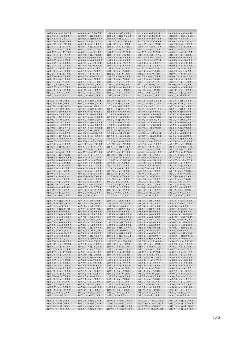
133

cpi2 % # -> cpi2 % # S R cp3 % # -> cp3 % # S R cpi3 % # -> cpi3 % # S R end % # -> end % # S R endi % # -> endi % # S R cpi2 % 0 -> cpi2 % 0 S R cp3 % 0 -> cp3 % 0 S R cpi3 % 0 -> cpi3 % 0 S R end % 0 -> end % 0 S R endi % 0 -> endi % 0 S R cpi2 % % -> re _ % L L cp3 % % -> cpi3 % % R R cpi3 % % -> re _ _ L L end % % -> endi % % R R endi % % -> cl % % L L cpi2 0' 0' -> q- 0' 0' R R cp3 0' 0' -> q- 0' 0' R R cpi3 0' 0' -> q- 0' 0' R R end 0' 0' -> q- 0' 0' R R endi 0' 0' -> q- 0' 0' R R cpi2 _' 0' -> q- _' 0' R R cp3 _' 0' -> q- _' 0' R R cpi3 _' 0' -> q- _' 0' R R end _' 0' -> q- _' 0' R R endi _' 0' -> q- _' 0' R R cpi2 % _' -> q- % _' R R cp3 % _' -> cp3 % _' S R cpi3 % _' -> q- % _' R R end % _' -> end % _' S R endi % _' -> q- % _' R R cpi2 _' _' -> q- _' _' R R cp3 _' _' -> q- _' _' R R cpi3 _' _' -> q- _' _' R R end _' _' -> q- _' _' R R endi _' _' -> q- _' _' R R cpi2 0' _' -> q- 0' _' R R cp3 0' _' -> q- 0' _' R R cpi3 0' _' -> q- 0' _' R R end 0' _' -> q- 0' _' R R endi 0' _' -> q- 0' _' R R cpi2 _' % -> q- _' % R R cp3 _' % -> cp3 _' % R S cpi3 _' % -> q- _' % R R end _' % -> end _' % R S endi _' % -> q- _' % R R cpi2 0' % -> q- 0' % R R cp3 0' % -> cp3 0' % R S cpi3 0' % -> q- 0' % R R end 0' % -> end 0' % R S endi 0' % -> q- 0' % R R cpi2 % 0' -> q- % 0' R R cp3 % 0' -> cp3 % 0' S R cpi3 % 0' -> q- % 0' R R end % 0' -> end % 0' S R endi % 0' -> q- % 0' R R cpi2 # 0' -> q- # 0' R R cp3 # 0' -> q- # 0' R R cpi3 # 0' -> q- # 0' R R end # 0' -> q- # 0' R R endi # 0' -> q- # 0' R R cpi2 0' # -> q- 0' # R R cp3 0' # -> q- 0' # R R cpi3 0' # -> q- 0' # R R end 0' # -> q- 0' # R R endi 0' # -> q- 0' # R R cpi2 # _' -> q- # _' R R cp3 # _' -> q- # _' R R cpi3 # _' -> q- # _' R R end # _' -> q- # _' R R endi # _' -> q- # _' R R cpi2 _' # -> q- _' # R R cp3 _' # -> q- _' # R R cpi3 _' # -> q- _' # R R end _' # -> q- _' # R R endi _' # -> q- _' # R R cpi2 0' _ -> q- 0' _ R R cp3 0' _ -> q- 0' _ R R cpi3 0' _ -> q- 0' _ R R end 0' _ -> q- 0' _ R R endi 0' _ -> q- 0' _ R R cpi2 0' 0 -> q- 0' 0 R R cp3 0' 0 -> q- 0' 0 R R cpi3 0' 0 -> q- 0' 0 R R end 0' 0 -> q- 0' 0 R R endi 0' 0 -> q- 0' 0 R R cpi2 _' 0 -> q- _' 0 R R cp3 _' 0 -> q- _' 0 R R cpi3 _' 0 -> q- _' 0 R R end _' 0 -> q- _' 0 R R endi _' 0 -> q- _' 0 R R cpi2 _' _ -> q- _' _ R R cp3 _' _ -> q- _' _ R R cpi3 _' _ -> q- _' _ R R end _' _ -> q- _' _ R R endi _' _ -> q- _' _ R R cpi2 0 _' -> q- 0 _' R R cp3 0 _' -> q- 0 _' R R cpi3 0 _' -> q- 0 _' R R end 0 _' -> q- 0 _' R R endi 0 _' -> q- 0 _' R R cpi2 0 0' -> q- 0 0' R R cp3 0 0' -> q- 0 0' R R cpi3 0 0' -> q- 0 0' R R end 0 0' -> q- 0 0' R R endi 0 0' -> q- 0 0' R R cpi2 _ 0' -> q- _ 0' R R cp3 _ 0' -> q- _ 0' R R cpi3 _ 0' -> q- _ 0' R R end _ 0' -> q- _ 0' R R endi _ 0' -> q- _ 0' R R cpi2 _ _' -> q- _ _' R R cp3 _ _' -> q- _ _' R R cpi3 _ _' -> q- _ _' R R end _ _' -> q- _ _' R R endi _ _' -> q- _ _' R R cpi2 _ _ -> re _ % L L cp3 _ _ -> cp3 _ _ R R cpi3 _ _ -> re _ _ L L end _ _ -> end _ _ R R endi _ _ -> cl % % L L cp4 _ # -> cp4 _ # R R cpi4 _ # -> cpi4 _ # S R cp5 _ # -> cp5 _ # R R cpi5 _ # -> cpi5 _ # S R cp6 _ # -> cp6 _ # R R cp4 _ 0 -> cp4 _ 0 R R cpi4 _ 0 -> cpi4 _ 0 S R cp5 _ 0 -> cp5 _ 0 R R cpi5 _ 0 -> cpi5 _ 0 S R cp6 _ 0 -> cp6 _ 0 R R cp4 _ % -> cp4 _ % R S cpi4 _ % -> re _ 0 L L cp5 _ % -> cp5 _ % R S cpi5 _ % -> re 0 _ L L cp6 _ % -> cp6 _ % R S cp4 # _ -> cp4 # _ R R cpi4 # _ -> cpi4 # _ R S cp5 # _ -> cp5 # _ R R cpi5 # _ -> cpi5 # _ R S cp6 # _ -> cp6 # _ R R cp4 # # -> cp4 # # R R cpi4 # # -> q- # # R R cp5 # # -> cp5 # # R R cpi5 # # -> q- # # R R cp6 # # -> cp6 # # R R cp4 # 0 -> cp4 # 0 R R cpi4 # 0 -> cpi4 # 0 R R cp5 # 0 -> cp5 # 0 R R cpi5 # 0 -> cpi5 # 0 R R cp6 # 0 -> cp6 # 0 R R cp4 # % -> cp4 # % R S cpi4 # % -> cpi4 # % R S cp5 # % -> cp5 # % R S cpi5 # % -> cpi5 # % R S cp6 # % -> cp6 # % R S cp4 0 _ -> cp4 0 _ R R cpi4 0 _ -> cpi4 0 _ R S cp5 0 _ -> cp5 0 _ R R cpi5 0 _ -> cpi5 0 _ R S cp6 0 _ -> cp6 0 _ R R cp4 0 # -> cp4 0 # R R cpi4 0 # -> cpi4 0 # R R cp5 0 # -> cp5 0 # R R cpi5 0 # -> cpi5 0 # R R cp6 0 # -> cp6 0 # R R cp4 0 0 -> cp4 0 0 R R cpi4 0 0 -> cpi4 0 0 R R cp5 0 0 -> cp5 0 0 R R cpi5 0 0 -> cpi5 0 0 R R cp6 0 0 -> cp6 0 0 R R cp4 0 % -> cp4 0 % R S cpi4 0 % -> cpi4 0 % R S cp5 0 % -> cp5 0 % R S cpi5 0 % -> cpi5 0 % R S cp6 0 % -> cp6 0 % R S cp4 % _ -> cp4 % _ S R cpi4 % _ -> re _ 0 L L cp5 % _ -> cp5 % _ S R cpi5 % _ -> re 0 _ L L cp6 % _ -> cp6 % _ S R cp4 % # -> cp4 % # S R cpi4 % # -> cpi4 % # S R cp5 % # -> cp5 % # S R cpi5 % # -> cpi5 % # S R cp6 % # -> cp6 % # S R cp4 % 0 -> cp4 % 0 S R cpi4 % 0 -> cpi4 % 0 S R cp5 % 0 -> cp5 % 0 S R cpi5 % 0 -> cpi5 % 0 S R cp6 % 0 -> cp6 % 0 S R cp4 % % -> cpi4 % % R R cpi4 % % -> re _ 0 L L cp5 % % -> cpi5 % % R R cpi5 % % -> re 0 _ L L cp6 % % -> cpi6 % % R R cp4 0' 0' -> q- 0' 0' R R cpi4 0' 0' -> q- 0' 0' R R cp5 0' 0' -> q- 0' 0' R R cpi5 0' 0' -> q- 0' 0' R R cp6 0' 0' -> q- 0' 0' R R cp4 _' 0' -> q- _' 0' R R cpi4 _' 0' -> q- _' 0' R R cp5 _' 0' -> q- _' 0' R R cpi5 _' 0' -> q- _' 0' R R cp6 _' 0' -> q- _' 0' R R cp4 % _' -> cp4 % _' S R cpi4 % _' -> q- % _' R R cp5 % _' -> cp5 % _' S R cpi5 % _' -> q- % _' R R cp6 % _' -> cp6 % _' S R cp4 _' _' -> q- _' _' R R cpi4 _' _' -> q- _' _' R R cp5 _' _' -> q- _' _' R R cpi5 _' _' -> q- _' _' R R cp6 _' _' -> q- _' _' R R cp4 0' _' -> q- 0' _' R R cpi4 0' _' -> q- 0' _' R R cp5 0' _' -> q- 0' _' R R cpi5 0' _' -> q- 0' _' R R cp6 0' _' -> q- 0' _' R R cp4 _' % -> cp4 _' % R S cpi4 _' % -> q- _' % R R cp5 _' % -> cp5 _' % R S cpi5 _' % -> q- _' % R R cp6 _' % -> cp6 _' % R S cp4 0' % -> cp4 0' % R S cpi4 0' % -> q- 0' % R R cp5 0' % -> cp5 0' % R S cpi5 0' % -> q- 0' % R R cp6 0' % -> cp6 0' % R S cp4 % 0' -> cp4 % 0' S R cpi4 % 0' -> q- % 0' R R cp5 % 0' -> cp5 % 0' S R cpi5 % 0' -> q- % 0' R R cp6 % 0' -> cp6 % 0' S R cp4 # 0' -> q- # 0' R R cpi4 # 0' -> q- # 0' R R cp5 # 0' -> q- # 0' R R cpi5 # 0' -> q- # 0' R R cp6 # 0' -> q- # 0' R R cp4 0' # -> q- 0' # R R cpi4 0' # -> q- 0' # R R cp5 0' # -> q- 0' # R R cpi5 0' # -> q- 0' # R R cp6 0' # -> q- 0' # R R cp4 # _' -> q- # _' R R cpi4 # _' -> q- # _' R R cp5 # _' -> q- # _' R R cpi5 # _' -> q- # _' R R cp6 # _' -> q- # _' R R cp4 _' # -> q- _' # R R cpi4 _' # -> q- _' # R R cp5 _' # -> q- _' # R R cpi5 _' # -> q- _' # R R cp6 _' # -> q- _' # R R cp4 0' _ -> q- 0' _ R R cpi4 0' _ -> q- 0' _ R R cp5 0' _ -> q- 0' _ R R cpi5 0' _ -> q- 0' _ R R cp6 0' _ -> q- 0' _ R R cp4 0' 0 -> q- 0' 0 R R cpi4 0' 0 -> q- 0' 0 R R cp5 0' 0 -> q- 0' 0 R R cpi5 0' 0 -> q- 0' 0 R R cp6 0' 0 -> q- 0' 0 R R cp4 _' 0 -> q- _' 0 R R cpi4 _' 0 -> q- _' 0 R R cp5 _' 0 -> q- _' 0 R R cpi5 _' 0 -> q- _' 0 R R cp6 _' 0 -> q- _' 0 R R cp4 _' _ -> q- _' _ R R cpi4 _' _ -> q- _' _ R R cp5 _' _ -> q- _' _ R R cpi5 _' _ -> q- _' _ R R cp6 _' _ -> q- _' _ R R cp4 0 _' -> q- 0 _' R R cpi4 0 _' -> q- 0 _' R R cp5 0 _' -> q- 0 _' R R cpi5 0 _' -> q- 0 _' R R cp6 0 _' -> q- 0 _' R R cp4 0 0' -> q- 0 0' R R cpi4 0 0' -> q- 0 0' R R cp5 0 0' -> q- 0 0' R R cpi5 0 0' -> q- 0 0' R R cp6 0 0' -> q- 0 0' R R cp4 _ 0' -> q- _ 0' R R cpi4 _ 0' -> q- _ 0' R R cp5 _ 0' -> q- _ 0' R R cpi5 _ 0' -> q- _ 0' R R cp6 _ 0' -> q- _ 0' R R cp4 _ _' -> q- _ _' R R cpi4 _ _' -> q- _ _' R R cp5 _ _' -> q- _ _' R R cpi5 _ _' -> q- _ _' R R cp6 _ _' -> q- _ _' R R cp4 _ _ -> cp4 _ _ R R cpi4 _ _ -> re _ 0 L L cp5 _ _ -> cp5 _ _ R R cpi5 _ _ -> re 0 _ L L cp6 _ _ -> cp6 _ _ R R cpi6 _ # -> cpi6 _ # S R cp7 _ # -> cp7 _ # R R cpi7 _ # -> cpi7 _ # S R cp8 _ # -> cp8 _ # R R cpi8 _ # -> cpi8 _ # S R cpi6 _ 0 -> cpi6 _ 0 S R cp7 _ 0 -> cp7 _ 0 R R cpi7 _ 0 -> cpi7 _ 0 S R cp8 _ 0 -> cp8 _ 0 R R cpi8 _ 0 -> cpi8 _ 0 S R cpi6 _ % -> re 0 _ L L cp7 _ % -> cp7 _ % R S cpi7 _ % -> re 0 0 L L cp8 _ % -> cp8 _ % R S cpi8 _ % -> re 0 % L L cpi6 # _ -> cpi6 # _ R S cp7 # _ -> cp7 # _ R R cpi7 # _ -> cpi7 # _ R S cp8 # _ -> cp8 # _ R R cpi8 # _ -> cpi8 # _ R S cpi6 # # -> q- # # R R cp7 # # -> cp7 # # R R cpi7 # # -> q- # # R R cp8 # # -> cp8 # # R R cpi8 # # -> q- # # R R cpi6 # 0 -> cpi6 # 0 R R cp7 # 0 -> cp7 # 0 R R cpi7 # 0 -> cpi7 # 0 R R cp8 # 0 -> cp8 # 0 R R cpi8 # 0 -> cpi8 # 0 R R cpi6 # % -> cpi6 # % R S cp7 # % -> cp7 # % R S cpi7 # % -> cpi7 # % R S cp8 # % -> cp8 # % R S cpi8 # % -> cpi8 # % R S cpi6 0 _ -> cpi6 0 _ R S cp7 0 _ -> cp7 0 _ R R cpi7 0 _ -> cpi7 0 _ R S cp8 0 _ -> cp8 0 _ R R cpi8 0 _ -> cpi8 0 _ R S cpi6 0 # -> cpi6 0 # R R cp7 0 # -> cp7 0 # R R cpi7 0 # -> cpi7 0 # R R cp8 0 # -> cp8 0 # R R cpi8 0 # -> cpi8 0 # R R cpi6 0 0 -> cpi6 0 0 R R cp7 0 0 -> cp7 0 0 R R cpi7 0 0 -> cpi7 0 0 R R cp8 0 0 -> cp8 0 0 R R cpi8 0 0 -> cpi8 0 0 R R cpi6 0 % -> cpi6 0 % R S cp7 0 % -> cp7 0 % R S cpi7 0 % -> cpi7 0 % R S cp8 0 % -> cp8 0 % R S cpi8 0 % -> cpi8 0 % R S cpi6 % _ -> re 0 _ L L cp7 % _ -> cp7 % _ S R cpi7 % _ -> re 0 0 L L cp8 % _ -> cp8 % _ S R cpi8 % _ -> re 0 % L L cpi6 % # -> cpi6 % # S R cp7 % # -> cp7 % # S R cpi7 % # -> cpi7 % # S R cp8 % # -> cp8 % # S R cpi8 % # -> cpi8 % # S R cpi6 % 0 -> cpi6 % 0 S R cp7 % 0 -> cp7 % 0 S R cpi7 % 0 -> cpi7 % 0 S R cp8 % 0 -> cp8 % 0 S R cpi8 % 0 -> cpi8 % 0 S R cpi6 % % -> re 0 _ L L cp7 % % -> cpi7 % % R R cpi7 % % -> re 0 0 L L cp8 % % -> cpi8 % % R R cpi8 % % -> re 0 % L L cpi6 0' 0' -> q- 0' 0' R R cp7 0' 0' -> q- 0' 0' R R cpi7 0' 0' -> q- 0' 0' R R cp8 0' 0' -> q- 0' 0' R R cpi8 0' 0' -> q- 0' 0' R R cpi6 _' 0' -> q- _' 0' R R cp7 _' 0' -> q- _' 0' R R cpi7 _' 0' -> q- _' 0' R R cp8 _' 0' -> q- _' 0' R R cpi8 _' 0' -> q- _' 0' R R cpi6 % _' -> q- % _' R R cp7 % _' -> cp7 % _' S R cpi7 % _' -> q- % _' R R cp8 % _' -> cp8 % _' S R cpi8 % _' -> q- % _' R R cpi6 _' _' -> q- _' _' R R cp7 _' _' -> q- _' _' R R cpi7 _' _' -> q- _' _' R R cp8 _' _' -> q- _' _' R R cpi8 _' _' -> q- _' _' R R cpi6 0' _' -> q- 0' _' R R cp7 0' _' -> q- 0' _' R R cpi7 0' _' -> q- 0' _' R R cp8 0' _' -> q- 0' _' R R cpi8 0' _' -> q- 0' _' R R cpi6 _' % -> q- _' % R R cp7 _' % -> cp7 _' % R S cpi7 _' % -> q- _' % R R cp8 _' % -> cp8 _' % R S cpi8 _' % -> q- _' % R R cpi6 0' % -> q- 0' % R R cp7 0' % -> cp7 0' % R S cpi7 0' % -> q- 0' % R R cp8 0' % -> cp8 0' % R S cpi8 0' % -> q- 0' % R R cpi6 % 0' -> q- % 0' R R cp7 % 0' -> cp7 % 0' S R cpi7 % 0' -> q- % 0' R R cp8 % 0' -> cp8 % 0' S R cpi8 % 0' -> q- % 0' R R cpi6 # 0' -> q- # 0' R R cp7 # 0' -> q- # 0' R R cpi7 # 0' -> q- # 0' R R cp8 # 0' -> q- # 0' R R cpi8 # 0' -> q- # 0' R R cpi6 0' # -> q- 0' # R R cp7 0' # -> q- 0' # R R cpi7 0' # -> q- 0' # R R cp8 0' # -> q- 0' # R R cpi8 0' # -> q- 0' # R R cpi6 # _' -> q- # _' R R cp7 # _' -> q- # _' R R cpi7 # _' -> q- # _' R R cp8 # _' -> q- # _' R R cpi8 # _' -> q- # _' R R cpi6 _' # -> q- _' # R R cp7 _' # -> q- _' # R R cpi7 _' # -> q- _' # R R cp8 _' # -> q- _' # R R cpi8 _' # -> q- _' # R R cpi6 0' _ -> q- 0' _ R R cp7 0' _ -> q- 0' _ R R cpi7 0' _ -> q- 0' _ R R cp8 0' _ -> q- 0' _ R R cpi8 0' _ -> q- 0' _ R R cpi6 0' 0 -> q- 0' 0 R R cp7 0' 0 -> q- 0' 0 R R cpi7 0' 0 -> q- 0' 0 R R cp8 0' 0 -> q- 0' 0 R R cpi8 0' 0 -> q- 0' 0 R R cpi6 _' 0 -> q- _' 0 R R cp7 _' 0 -> q- _' 0 R R cpi7 _' 0 -> q- _' 0 R R cp8 _' 0 -> q- _' 0 R R cpi8 _' 0 -> q- _' 0 R R cpi6 _' _ -> q- _' _ R R cp7 _' _ -> q- _' _ R R cpi7 _' _ -> q- _' _ R R cp8 _' _ -> q- _' _ R R cpi8 _' _ -> q- _' _ R R cpi6 0 _' -> q- 0 _' R R cp7 0 _' -> q- 0 _' R R cpi7 0 _' -> q- 0 _' R R cp8 0 _' -> q- 0 _' R R cpi8 0 _' -> q- 0 _' R R cpi6 0 0' -> q- 0 0' R R cp7 0 0' -> q- 0 0' R R cpi7 0 0' -> q- 0 0' R R cp8 0 0' -> q- 0 0' R R cpi8 0 0' -> q- 0 0' R R cpi6 _ 0' -> q- _ 0' R R cp7 _ 0' -> q- _ 0' R R cpi7 _ 0' -> q- _ 0' R R cp8 _ 0' -> q- _ 0' R R cpi8 _ 0' -> q- _ 0' R R cpi6 _ _' -> q- _ _' R R cp7 _ _' -> q- _ _' R R cpi7 _ _' -> q- _ _' R R cp8 _ _' -> q- _ _' R R cpi8 _ _' -> q- _ _' R R cpi6 _ _ -> re 0 _ L L cp7 _ _ -> cp7 _ _ R R cpi7 _ _ -> re 0 0 L L cp8 _ _ -> cp8 _ _ R R cpi8 _ _ -> re 0 % L L cp9 _ # -> cp9 _ # R R cpi9 _ # -> cpi9 _ # S R cp10 _ # -> cp10 _ # R R cpi10 _ # -> cpi10 _ # S R cp11 _ # -> cp11 _ # R R cp9 _ 0 -> cp9 _ 0 R R cpi9 _ 0 -> cpi9 _ 0 S R cp10 _ 0 -> cp10 _ 0 R R cpi10 _ 0 -> cpi10 _ 0 S R cp11 _ 0 -> cp11 _ 0 R R cp9 _ % -> cp9 _ % R S cpi9 _ % -> re % _ L L cp10 _ % -> cp10 _ % R S cpi10 _ % -> re % 0 L L cp11 _ % -> cp11 _ % R S cp9 # _ -> cp9 # _ R R cpi9 # _ -> cpi9 # _ R S cp10 # _ -> cp10 # _ R R cpi10 # _ -> cpi10 # _ R S cp11 # _ -> cp11 # _ R R

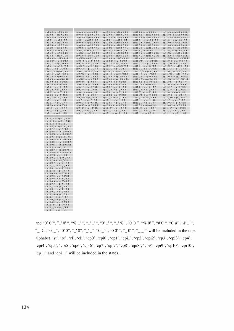
134

cp9 # # -> cp9 # # R R cpi9 # # -> q- # # R R cp10 # # -> cp10 # # R R cpi10 # # -> q- # # R R cp11 # # -> cp11 # # R R cp9 # 0 -> cp9 # 0 R R cpi9 # 0 -> cpi9 # 0 R R cp10 # 0 -> cp10 # 0 R R cpi10 # 0 -> cpi10 # 0 R R cp11 # 0 -> cp11 # 0 R R cp9 # % -> cp9 # % R S cpi9 # % -> cpi9 # % R S cp10 # % -> cp10 # % R S cpi10 # % -> cpi10 # % R S cp11 # % -> cp11 # % R S cp9 0 _ -> cp9 0 _ R R cpi9 0 _ -> cpi9 0 _ R S cp10 0 _ -> cp10 0 _ R R cpi10 0 _ -> cpi10 0 _ R S cp11 0 _ -> cp11 0 _ R R cp9 0 # -> cp9 0 # R R cpi9 0 # -> cpi9 0 # R R cp10 0 # -> cp10 0 # R R cpi10 0 # -> cpi10 0 # R R cp11 0 # -> cp11 0 # R R cp9 0 0 -> cp9 0 0 R R cpi9 0 0 -> cpi9 0 0 R R cp10 0 0 -> cp10 0 0 R R cpi10 0 0 -> cpi10 0 0 R R cp11 0 0 -> cp11 0 0 R R cp9 0 % -> cp9 0 % R S cpi9 0 % -> cpi9 0 % R S cp10 0 % -> cp10 0 % R S cpi10 0 % -> cpi10 0 % R S cp11 0 % -> cp11 0 % R S cp9 % _ -> cp9 % _ S R cpi9 % _ -> re % _ L L cp10 % _ -> cp10 % _ S R cpi10 % _ -> re % 0 L L cp11 % _ -> cp11 % _ S R cp9 % # -> cp9 % # S R cpi9 % # -> cpi9 % # S R cp10 % # -> cp10 % # S R cpi10 % # -> cpi10 % # S R cp11 % # -> cp11 % # S R cp9 % 0 -> cp9 % 0 S R cpi9 % 0 -> cpi9 % 0 S R cp10 % 0 -> cp10 % 0 S R cpi10 % 0 -> cpi10 % 0 S R cp11 % 0 -> cp11 % 0 S R cp9 % % -> cpi9 % % R R cpi9 % % -> re % _ L L cp10 % % -> cpi10 % % R R cpi10 % % -> re % 0 L L cp11 % % -> cpi11 % % R R cp9 0' 0' -> q- 0' 0' R R cpi9 0' 0' -> q- 0' 0' R R cp10 0' 0' -> q- 0' 0' R R cpi10 0' 0' -> q- 0' 0' R R cp11 0' 0' -> q- 0' 0' R R cp9 _' 0' -> q- _' 0' R R cpi9 _' 0' -> q- _' 0' R R cp10 _' 0' -> q- _' 0' R R cpi10 _' 0' -> q- _' 0' R R cp11 _' 0' -> q- _' 0' R R cp9 % _' -> cp9 % _' S R cpi9 % _' -> q- % _' R R cp10 % _' -> cp10 % _' S R cpi10 % _' -> q- % _' R R cp11 % _' -> cp11 % _' S R cp9 _' _' -> q- _' _' R R cpi9 _' _' -> q- _' _' R R cp10 _' _' -> q- _' _' R R cpi10 _' _' -> q- _' _' R R cp11 _' _' -> q- _' _' R R cp9 0' _' -> q- 0' _' R R cpi9 0' _' -> q- 0' _' R R cp10 0' _' -> q- 0' _' R R cpi10 0' _' -> q- 0' _' R R cp11 0' _' -> q- 0' _' R R cp9 _' % -> cp9 _' % R S cpi9 _' % -> q- _' % R R cp10 _' % -> cp10 _' % R S cpi10 _' % -> q- _' % R R cp11 _' % -> cp11 _' % R S cp9 0' % -> cp9 0' % R S cpi9 0' % -> q- 0' % R R cp10 0' % -> cp10 0' % R S cpi10 0' % -> q- 0' % R R cp11 0' % -> cp11 0' % R S cp9 % 0' -> cp9 % 0' S R cpi9 % 0' -> q- % 0' R R cp10 % 0' -> cp10 % 0' S R cpi10 % 0' -> q- % 0' R R cp11 % 0' -> cp11 % 0' S R cp9 # 0' -> q- # 0' R R cpi9 # 0' -> q- # 0' R R cp10 # 0' -> q- # 0' R R cpi10 # 0' -> q- # 0' R R cp11 # 0' -> q- # 0' R R cp9 0' # -> q- 0' # R R cpi9 0' # -> q- 0' # R R cp10 0' # -> q- 0' # R R cpi10 0' # -> q- 0' # R R cp11 0' # -> q- 0' # R R cp9 # _' -> q- # _' R R cpi9 # _' -> q- # _' R R cp10 # _' -> q- # _' R R cpi10 # _' -> q- # _' R R cp11 # _' -> q- # _' R R cp9 _' # -> q- _' # R R cpi9 _' # -> q- _' # R R cp10 _' # -> q- _' # R R cpi10 _' # -> q- _' # R R cp11 _' # -> q- _' # R R cp9 0' _ -> q- 0' _ R R cpi9 0' _ -> q- 0' _ R R cp10 0' _ -> q- 0' _ R R cpi10 0' _ -> q- 0' _ R R cp11 0' _ -> q- 0' _ R R cp9 0' 0 -> q- 0' 0 R R cpi9 0' 0 -> q- 0' 0 R R cp10 0' 0 -> q- 0' 0 R R cpi10 0' 0 -> q- 0' 0 R R cp11 0' 0 -> q- 0' 0 R R cp9 _' 0 -> q- _' 0 R R cpi9 _' 0 -> q- _' 0 R R cp10 _' 0 -> q- _' 0 R R cpi10 _' 0 -> q- _' 0 R R cp11 _' 0 -> q- _' 0 R R cp9 _' _ -> q- _' _ R R cpi9 _' _ -> q- _' _ R R cp10 _' _ -> q- _' _ R R cpi10 _' _ -> q- _' _ R R cp11 _' _ -> q- _' _ R R cp9 0 _' -> q- 0 _' R R cpi9 0 _' -> q- 0 _' R R cp10 0 _' -> q- 0 _' R R cpi10 0 _' -> q- 0 _' R R cp11 0 _' -> q- 0 _' R R cp9 0 0' -> q- 0 0' R R cpi9 0 0' -> q- 0 0' R R cp10 0 0' -> q- 0 0' R R cpi10 0 0' -> q- 0 0' R R cp11 0 0' -> q- 0 0' R R cp9 _ 0' -> q- _ 0' R R cpi9 _ 0' -> q- _ 0' R R cp10 _ 0' -> q- _ 0' R R cpi10 _ 0' -> q- _ 0' R R cp11 _ 0' -> q- _ 0' R R cp9 _ _' -> q- _ _' R R cpi9 _ _' -> q- _ _' R R cp10 _ _' -> q- _ _' R R cpi10 _ _' -> q- _ _' R R cp11 _ _' -> q- _ _' R R cp9 _ _ -> cp9 _ _ R R cpi9 _ _ -> re % _ L L cp10 _ _ -> cp10 _ _ R R cpi10 _ _ -> re % 0 L L cp11 _ _ -> cp11 _ _ R R cpi11 _ # -> cpi11 _ # S R cpi11 _ 0 -> cpi11 _ 0 S R cpi11 _ % -> re _ _ L L cpi11 # _ -> cpi11 # _ R S cpi11 # # -> q- # # R R cpi11 # 0 -> cpi11 # 0 R R cpi11 # % -> cpi11 # % R S cpi11 0 _ -> cpi11 0 _ R S cpi11 0 # -> cpi11 0 # R R cpi11 0 0 -> cpi11 0 0 R R cpi11 0 % -> cpi11 0 % R S cpi11 % _ -> re _ _ L L cpi11 % # -> cpi11 % # S R cpi11 % 0 -> cpi11 % 0 S R cpi11 % % -> re _ _ L L cpi11 0' 0' -> q- 0' 0' R R cpi11 _' 0' -> q- _' 0' R R cpi11 % _' -> q- % _' R R cpi11 _' _' -> q- _' _' R R cpi11 0' _' -> q- 0' _' R R cpi11 _' % -> q- _' % R R cpi11 0' % -> q- 0' % R R cpi11 % 0' -> q- % 0' R R cpi11 # 0' -> q- # 0' R R cpi11 0' # -> q- 0' # R R cpi11 # _' -> q- # _' R R cpi11 _' # -> q- _' # R R cpi11 0' _ -> q- 0' _ R R cpi11 0' 0 -> q- 0' 0 R R cpi11 _' 0 -> q- _' 0 R R cpi11 _' _ -> q- _' _ R R cpi11 0 _' -> q- 0 _' R R cpi11 0 0' -> q- 0 0' R R cpi11 _ 0' -> q- _ 0' R R cpi11 _ _' -> q- _ _' R R cpi11 _ _ -> re _ _ L L

and “0’ 0’“, ”_' 0' “, “% _' “, “_' _' “, “0' _' “, “_' %”, “0' %”, “% 0' ”, “# 0' “, “0' #”, “# _' “,

“_' #”, “0' _”, “0' 0”, “_' 0”, “_' _”, “0 _' “, “0 0' “, “_ 0' “, “_ _' “ will be included in the tape

alphabet. ‘st’, ‘re’, ‘cl’, ‘cli’, ‘cp0’, ‘cpi0’, ‘cp1’, ‘cpi1’, ‘cp2’, ‘cpi2’, ‘cp3’, ‘cpi3’, ‘cp4’,

‘cpi4’, ‘cp5’, ‘cpi5’, ‘cp6’, ‘cpi6’, ‘cp7’, ‘cpi7’, ‘cp8’, ‘cpi8’, ‘cp9’, ‘cpi9’, ‘cp10’, ‘cpi10’,

‘cp11’ and ‘cpi11’ will be included in the states.

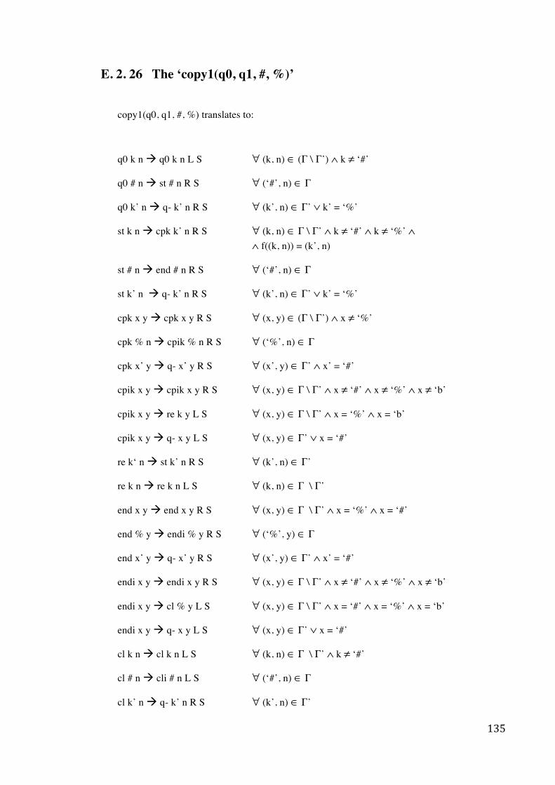
135

E. 2. 26 The ‘copy1(q0, q1, #, %)’

copy1(q0, q1, #, %) translates to:

q0 k n q0 k n L S ∀ (k, n) ∈ (Γ \ Γ’) ∧ k ≠ ‘#’

q0 # n st # n R S ∀ (‘#’, n) ∈ Γ

q0 k’ n q- k’ n R S ∀ (k’, n) ∈ Γ’ ∨ k’ = ‘%’

st k n cpk k’ n R S ∀ (k, n) ∈ Γ \ Γ’ ∧ k ≠ ‘#’ ∧ k ≠ ‘%’ ∧ ∧ f((k, n)) = (k’, n)

st # n end # n R S ∀ (‘#’, n) ∈ Γ

st k’ n q- k’ n R S ∀ (k’, n) ∈ Γ’ ∨ k’ = ‘%’

cpk x y cpk x y R S ∀ (x, y) ∈ (Γ \ Γ’) ∧ x ≠ ‘%’

cpk % n cpik % n R S ∀ (‘%’, n) ∈ Γ

cpk x’ y q- x’ y R S ∀ (x’, y) ∈ Γ’ ∧ x’ = ‘#’

cpik x y cpik x y R S ∀ (x, y) ∈ Γ \ Γ’ ∧ x ≠ ‘#’ ∧ x ≠ ‘%’ ∧ x ≠ ‘b’

cpik x y re k y L S ∀ (x, y) ∈ Γ \ Γ’ ∧ x = ‘%’ ∧ x = ‘b’

cpik x y q- x y L S ∀ (x, y) ∈ Γ’ ∨ x = ‘#’

re k‘ n st k’ n R S ∀ (k’, n) ∈ Γ’

re k n re k n L S ∀ (k, n) ∈ Γ \ Γ’

end x y end x y R S ∀ (x, y) ∈ Γ \ Γ’ ∧ x = ‘%’ ∧ x = ‘#’

end % y endi % y R S ∀ (‘%’, y) ∈ Γ

end x’ y q- x’ y R S ∀ (x’, y) ∈ Γ’ ∧ x’ = ‘#’

endi x y endi x y R S ∀ (x, y) ∈ Γ \ Γ’ ∧ x ≠ ‘#’ ∧ x ≠ ‘%’ ∧ x ≠ ‘b’

endi x y cl % y L S ∀ (x, y) ∈ Γ \ Γ’ ∧ x = ‘#’ ∧ x = ‘%’ ∧ x = ‘b’

endi x y q- x y L S ∀ (x, y) ∈ Γ’ ∨ x = ‘#’

cl k n cl k n L S ∀ (k, n) ∈ Γ \ Γ’ ∧ k ≠ ‘#’

cl # n cli # n L S ∀ (‘#’, n) ∈ Γ

cl k’ n q- k’ n R S ∀ (k’, n) ∈ Γ’

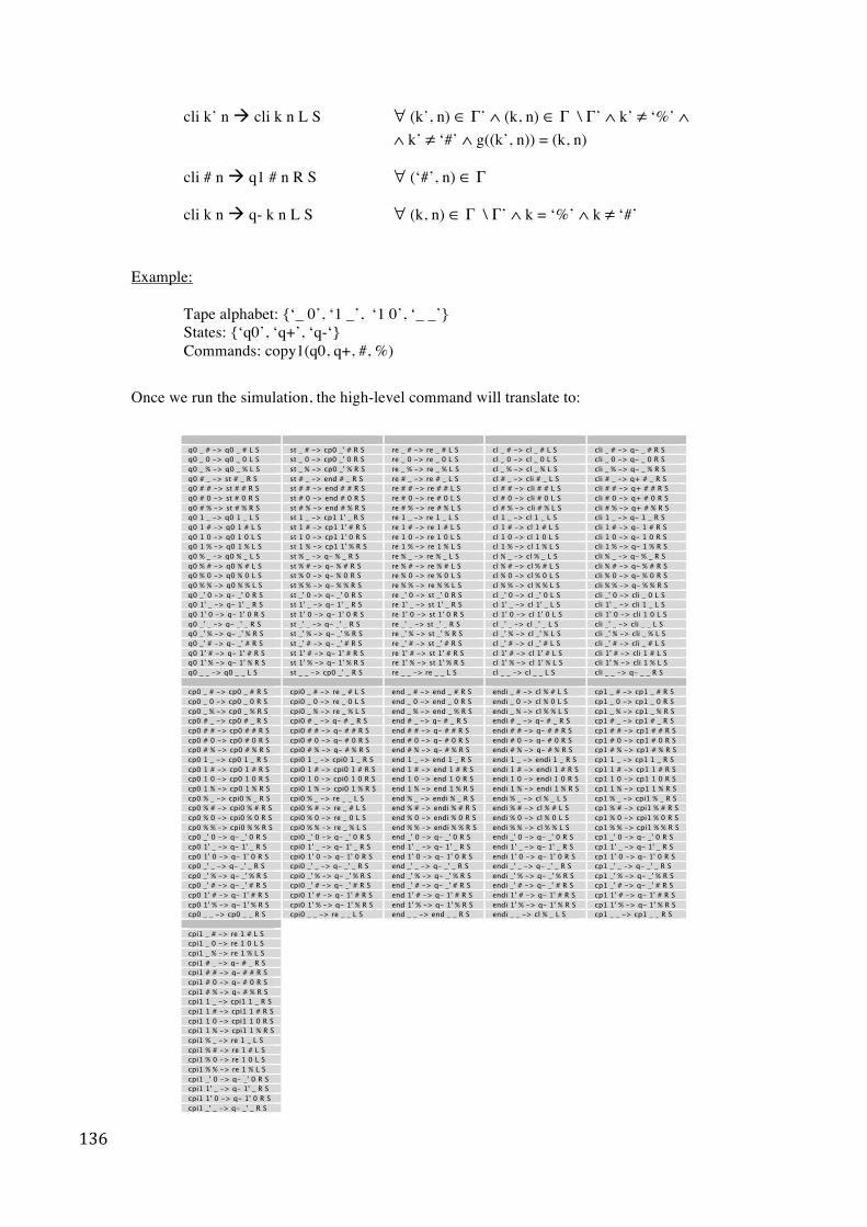
136

cli k’ n cli k n L S ∀ (k’, n) ∈ Γ’ ∧ (k, n) ∈ Γ \ Γ’ ∧ k’ ≠ ‘%’ ∧ ∧ k’ ≠ ‘#’ ∧ g((k’, n)) = (k, n)

cli # n q1 # n R S ∀ (‘#’, n) ∈ Γ

cli k n q- k n L S ∀ (k, n) ∈ Γ \ Γ’ ∧ k = ‘%’ ∧ k ≠ ‘#’


Commands: copy1(q0, q+, #, %)


q0 _ # -> q0 _ # L S st _ # -> cp0 _' # R S re _ # -> re _ # L S cl _ # -> cl _ # L S cli _ # -> q- _ # R S q0 _ 0 -> q0 _ 0 L S st _ 0 -> cp0 _' 0 R S re _ 0 -> re _ 0 L S cl _ 0 -> cl _ 0 L S cli _ 0 -> q- _ 0 R S q0 _ % -> q0 _ % L S st _ % -> cp0 _' % R S re _ % -> re _ % L S cl _ % -> cl _ % L S cli _ % -> q- _ % R S q0 # _ -> st # _ R S st # _ -> end # _ R S re # _ -> re # _ L S cl # _ -> cli # _ L S cli # _ -> q+ # _ R S q0 # # -> st # # R S st # # -> end # # R S re # # -> re # # L S cl # # -> cli # # L S cli # # -> q+ # # R S q0 # 0 -> st # 0 R S st # 0 -> end # 0 R S re # 0 -> re # 0 L S cl # 0 -> cli # 0 L S cli # 0 -> q+ # 0 R S q0 # % -> st # % R S st # % -> end # % R S re # % -> re # % L S cl # % -> cli # % L S cli # % -> q+ # % R S q0 1 _ -> q0 1 _ L S st 1 _ -> cp1 1' _ R S re 1 _ -> re 1 _ L S cl 1 _ -> cl 1 _ L S cli 1 _ -> q- 1 _ R S q0 1 # -> q0 1 # L S st 1 # -> cp1 1' # R S re 1 # -> re 1 # L S cl 1 # -> cl 1 # L S cli 1 # -> q- 1 # R S q0 1 0 -> q0 1 0 L S st 1 0 -> cp1 1' 0 R S re 1 0 -> re 1 0 L S cl 1 0 -> cl 1 0 L S cli 1 0 -> q- 1 0 R S q0 1 % -> q0 1 % L S st 1 % -> cp1 1' % R S re 1 % -> re 1 % L S cl 1 % -> cl 1 % L S cli 1 % -> q- 1 % R S q0 % _ -> q0 % _ L S st % _ -> q- % _ R S re % _ -> re % _ L S cl % _ -> cl % _ L S cli % _ -> q- % _ R S q0 % # -> q0 % # L S st % # -> q- % # R S re % # -> re % # L S cl % # -> cl % # L S cli % # -> q- % # R S q0 % 0 -> q0 % 0 L S st % 0 -> q- % 0 R S re % 0 -> re % 0 L S cl % 0 -> cl % 0 L S cli % 0 -> q- % 0 R S q0 % % -> q0 % % L S st % % -> q- % % R S re % % -> re % % L S cl % % -> cl % % L S cli % % -> q- % % R S q0 _' 0 -> q- _' 0 R S st _' 0 -> q- _' 0 R S re _' 0 -> st _' 0 R S cl _' 0 -> cl _' 0 L S cli _' 0 -> cli _ 0 L S q0 1' _ -> q- 1' _ R S st 1' _ -> q- 1' _ R S re 1' _ -> st 1' _ R S cl 1' _ -> cl 1' _ L S cli 1' _ -> cli 1 _ L S q0 1' 0 -> q- 1' 0 R S st 1' 0 -> q- 1' 0 R S re 1' 0 -> st 1' 0 R S cl 1' 0 -> cl 1' 0 L S cli 1' 0 -> cli 1 0 L S q0 _' _ -> q- _' _ R S st _' _ -> q- _' _ R S re _' _ -> st _' _ R S cl _' _ -> cl _' _ L S cli _' _ -> cli _ _ L S q0 _' % -> q- _' % R S st _' % -> q- _' % R S re _' % -> st _' % R S cl _' % -> cl _' % L S cli _' % -> cli _ % L S q0 _' # -> q- _' # R S st _' # -> q- _' # R S re _' # -> st _' # R S cl _' # -> cl _' # L S cli _' # -> cli _ # L S q0 1' # -> q- 1' # R S st 1' # -> q- 1' # R S re 1' # -> st 1' # R S cl 1' # -> cl 1' # L S cli 1' # -> cli 1 # L S q0 1' % -> q- 1' % R S st 1' % -> q- 1' % R S re 1' % -> st 1' % R S cl 1' % -> cl 1' % L S cli 1' % -> cli 1 % L S q0 _ _ -> q0 _ _ L S st _ _ -> cp0 _' _ R S re _ _ -> re _ _ L S cl _ _ -> cl _ _ L S cli _ _ -> q- _ _ R S cp0 _ # -> cp0 _ # R S cpi0 _ # -> re _ # L S end _ # -> end _ # R S endi _ # -> cl % # L S cp1 _ # -> cp1 _ # R S cp0 _ 0 -> cp0 _ 0 R S cpi0 _ 0 -> re _ 0 L S end _ 0 -> end _ 0 R S endi _ 0 -> cl % 0 L S cp1 _ 0 -> cp1 _ 0 R S cp0 _ % -> cp0 _ % R S cpi0 _ % -> re _ % L S end _ % -> end _ % R S endi _ % -> cl % % L S cp1 _ % -> cp1 _ % R S cp0 # _ -> cp0 # _ R S cpi0 # _ -> q- # _ R S end # _ -> q- # _ R S endi # _ -> q- # _ R S cp1 # _ -> cp1 # _ R S cp0 # # -> cp0 # # R S cpi0 # # -> q- # # R S end # # -> q- # # R S endi # # -> q- # # R S cp1 # # -> cp1 # # R S cp0 # 0 -> cp0 # 0 R S cpi0 # 0 -> q- # 0 R S end # 0 -> q- # 0 R S endi # 0 -> q- # 0 R S cp1 # 0 -> cp1 # 0 R S cp0 # % -> cp0 # % R S cpi0 # % -> q- # % R S end # % -> q- # % R S endi # % -> q- # % R S cp1 # % -> cp1 # % R S cp0 1 _ -> cp0 1 _ R S cpi0 1 _ -> cpi0 1 _ R S end 1 _ -> end 1 _ R S endi 1 _ -> endi 1 _ R S cp1 1 _ -> cp1 1 _ R S cp0 1 # -> cp0 1 # R S cpi0 1 # -> cpi0 1 # R S end 1 # -> end 1 # R S endi 1 # -> endi 1 # R S cp1 1 # -> cp1 1 # R S cp0 1 0 -> cp0 1 0 R S cpi0 1 0 -> cpi0 1 0 R S end 1 0 -> end 1 0 R S endi 1 0 -> endi 1 0 R S cp1 1 0 -> cp1 1 0 R S cp0 1 % -> cp0 1 % R S cpi0 1 % -> cpi0 1 % R S end 1 % -> end 1 % R S endi 1 % -> endi 1 % R S cp1 1 % -> cp1 1 % R S cp0 % _ -> cpi0 % _ R S cpi0 % _ -> re _ _ L S end % _ -> endi % _ R S endi % _ -> cl % _ L S cp1 % _ -> cpi1 % _ R S cp0 % # -> cpi0 % # R S cpi0 % # -> re _ # L S end % # -> endi % # R S endi % # -> cl % # L S cp1 % # -> cpi1 % # R S cp0 % 0 -> cpi0 % 0 R S cpi0 % 0 -> re _ 0 L S end % 0 -> endi % 0 R S endi % 0 -> cl % 0 L S cp1 % 0 -> cpi1 % 0 R S cp0 % % -> cpi0 % % R S cpi0 % % -> re _ % L S end % % -> endi % % R S endi % % -> cl % % L S cp1 % % -> cpi1 % % R S cp0 _' 0 -> q- _' 0 R S cpi0 _' 0 -> q- _' 0 R S end _' 0 -> q- _' 0 R S endi _' 0 -> q- _' 0 R S cp1 _' 0 -> q- _' 0 R S cp0 1' _ -> q- 1' _ R S cpi0 1' _ -> q- 1' _ R S end 1' _ -> q- 1' _ R S endi 1' _ -> q- 1' _ R S cp1 1' _ -> q- 1' _ R S cp0 1' 0 -> q- 1' 0 R S cpi0 1' 0 -> q- 1' 0 R S end 1' 0 -> q- 1' 0 R S endi 1' 0 -> q- 1' 0 R S cp1 1' 0 -> q- 1' 0 R S cp0 _' _ -> q- _' _ R S cpi0 _' _ -> q- _' _ R S end _' _ -> q- _' _ R S endi _' _ -> q- _' _ R S cp1 _' _ -> q- _' _ R S cp0 _' % -> q- _' % R S cpi0 _' % -> q- _' % R S end _' % -> q- _' % R S endi _' % -> q- _' % R S cp1 _' % -> q- _' % R S cp0 _' # -> q- _' # R S cpi0 _' # -> q- _' # R S end _' # -> q- _' # R S endi _' # -> q- _' # R S cp1 _' # -> q- _' # R S cp0 1' # -> q- 1' # R S cpi0 1' # -> q- 1' # R S end 1' # -> q- 1' # R S endi 1' # -> q- 1' # R S cp1 1' # -> q- 1' # R S cp0 1' % -> q- 1' % R S cpi0 1' % -> q- 1' % R S end 1' % -> q- 1' % R S endi 1' % -> q- 1' % R S cp1 1' % -> q- 1' % R S cp0 _ _ -> cp0 _ _ R S cpi0 _ _ -> re _ _ L S end _ _ -> end _ _ R S endi _ _ -> cl % _ L S cp1 _ _ -> cp1 _ _ R S cpi1 _ # -> re 1 # L S cpi1 _ 0 -> re 1 0 L S cpi1 _ % -> re 1 % L S cpi1 # _ -> q- # _ R S cpi1 # # -> q- # # R S cpi1 # 0 -> q- # 0 R S cpi1 # % -> q- # % R S cpi1 1 _ -> cpi1 1 _ R S cpi1 1 # -> cpi1 1 # R S cpi1 1 0 -> cpi1 1 0 R S cpi1 1 % -> cpi1 1 % R S cpi1 % _ -> re 1 _ L S cpi1 % # -> re 1 # L S cpi1 % 0 -> re 1 0 L S cpi1 % % -> re 1 % L S cpi1 _' 0 -> q- _' 0 R S cpi1 1' _ -> q- 1' _ R S cpi1 1' 0 -> q- 1' 0 R S cpi1 _' _ -> q- _' _ R S

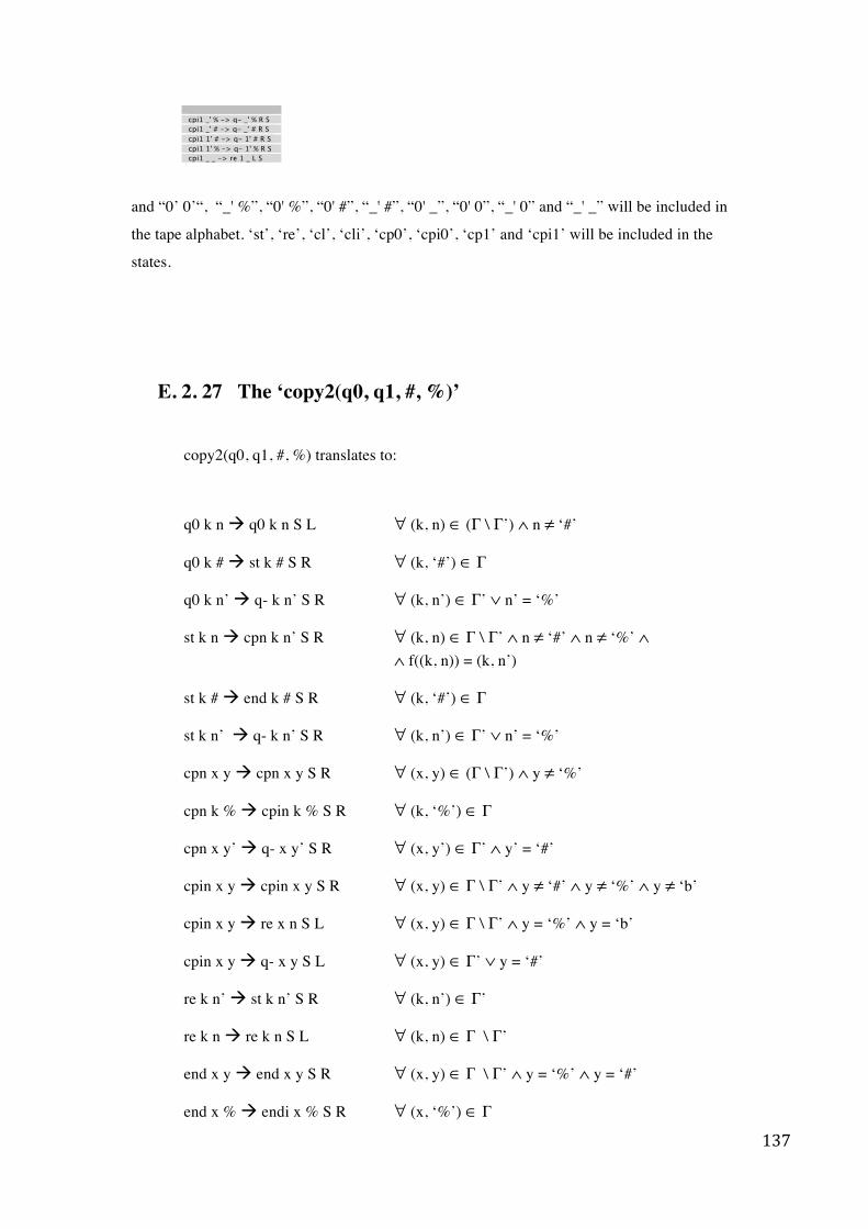
137

cpi1 _' % -> q- _' % R S cpi1 _' # -> q- _' # R S cpi1 1' # -> q- 1' # R S cpi1 1' % -> q- 1' % R S cpi1 _ _ -> re 1 _ L S

and “0’ 0’“, “_' %”, “0' %”, “0' #”, “_' #”, “0' _”, “0' 0”, “_' 0” and “_' _” will be included in

the tape alphabet. ‘st’, ‘re’, ‘cl’, ‘cli’, ‘cp0’, ‘cpi0’, ‘cp1’ and ‘cpi1’ will be included in the

states.

E. 2. 27 The ‘copy2(q0, q1, #, %)’

copy2(q0, q1, #, %) translates to:

q0 k n q0 k n S L ∀ (k, n) ∈ (Γ \ Γ’) ∧ n ≠ ‘#’

q0 k # st k # S R ∀ (k, ‘#’) ∈ Γ

q0 k n’ q- k n’ S R ∀ (k, n’) ∈ Γ’ ∨ n’ = ‘%’

st k n cpn k n’ S R ∀ (k, n) ∈ Γ \ Γ’ ∧ n ≠ ‘#’ ∧ n ≠ ‘%’ ∧ ∧ f((k, n)) = (k, n’)

st k # end k # S R ∀ (k, ‘#’) ∈ Γ

st k n’ q- k n’ S R ∀ (k, n’) ∈ Γ’ ∨ n’ = ‘%’

cpn x y cpn x y S R ∀ (x, y) ∈ (Γ \ Γ’) ∧ y ≠ ‘%’

cpn k % cpin k % S R ∀ (k, ‘%’) ∈ Γ

cpn x y’ q- x y’ S R ∀ (x, y’) ∈ Γ’ ∧ y’ = ‘#’

cpin x y cpin x y S R ∀ (x, y) ∈ Γ \ Γ’ ∧ y ≠ ‘#’ ∧ y ≠ ‘%’ ∧ y ≠ ‘b’

cpin x y re x n S L ∀ (x, y) ∈ Γ \ Γ’ ∧ y = ‘%’ ∧ y = ‘b’

cpin x y q- x y S L ∀ (x, y) ∈ Γ’ ∨ y = ‘#’

re k n’ st k n’ S R ∀ (k, n’) ∈ Γ’

re k n re k n S L ∀ (k, n) ∈ Γ \ Γ’

end x y end x y S R ∀ (x, y) ∈ Γ \ Γ’ ∧ y = ‘%’ ∧ y = ‘#’

end x % endi x % S R ∀ (x, ‘%’) ∈ Γ

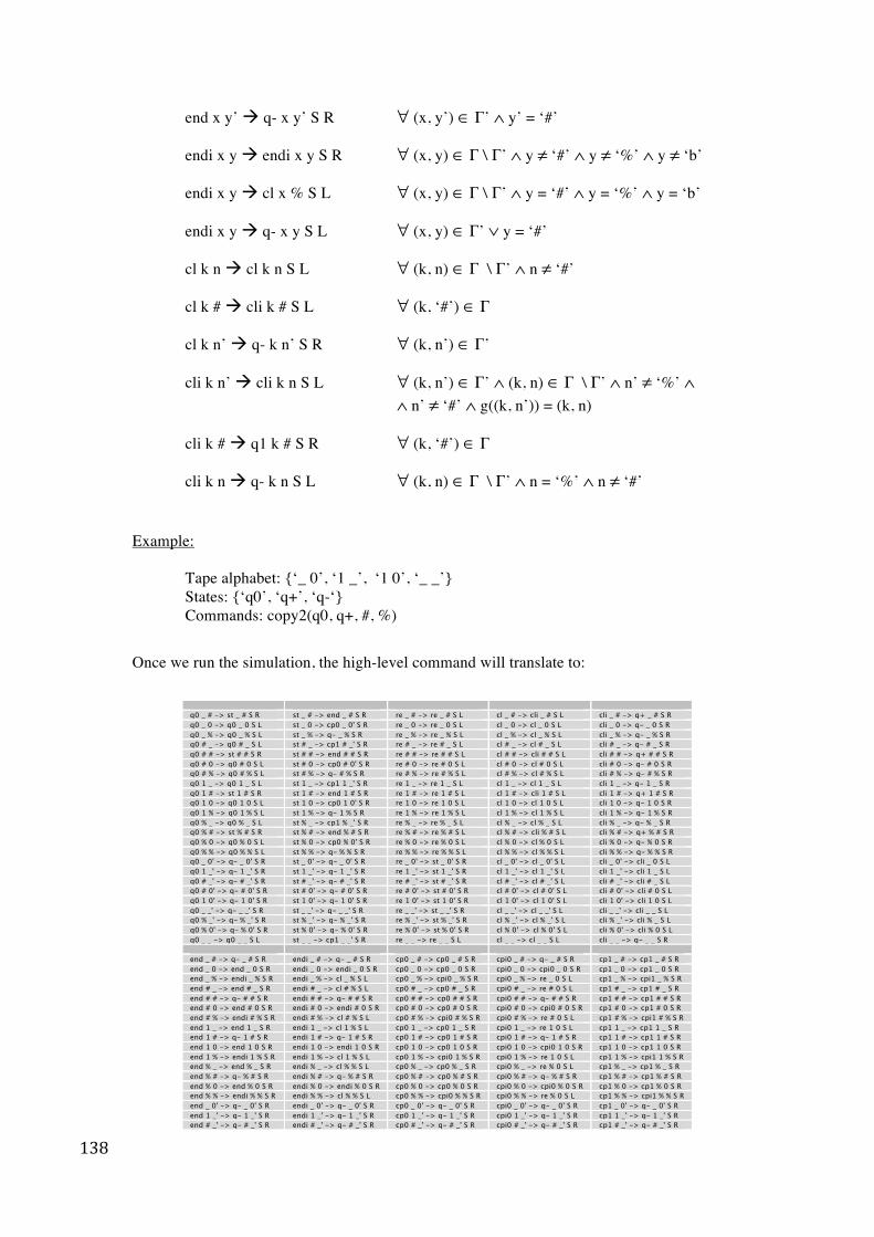
138

end x y’ q- x y’ S R ∀ (x, y’) ∈ Γ’ ∧ y’ = ‘#’

endi x y endi x y S R ∀ (x, y) ∈ Γ \ Γ’ ∧ y ≠ ‘#’ ∧ y ≠ ‘%’ ∧ y ≠ ‘b’

endi x y cl x % S L ∀ (x, y) ∈ Γ \ Γ’ ∧ y = ‘#’ ∧ y = ‘%’ ∧ y = ‘b’

endi x y q- x y S L ∀ (x, y) ∈ Γ’ ∨ y = ‘#’

cl k n cl k n S L ∀ (k, n) ∈ Γ \ Γ’ ∧ n ≠ ‘#’

cl k # cli k # S L ∀ (k, ‘#’) ∈ Γ

cl k n’ q- k n’ S R ∀ (k, n’) ∈ Γ’

cli k n’ cli k n S L ∀ (k, n’) ∈ Γ’ ∧ (k, n) ∈ Γ \ Γ’ ∧ n’ ≠ ‘%’ ∧ ∧ n’ ≠ ‘#’ ∧ g((k, n’)) = (k, n)

cli k # q1 k # S R ∀ (k, ‘#’) ∈ Γ

cli k n q- k n S L ∀ (k, n) ∈ Γ \ Γ’ ∧ n = ‘%’ ∧ n ≠ ‘#’


Commands: copy2(q0, q+, #, %)


q0 _ # -> st _ # S R st _ # -> end _ # S R re _ # -> re _ # S L cl _ # -> cli _ # S L cli _ # -> q+ _ # S R q0 _ 0 -> q0 _ 0 S L st _ 0 -> cp0 _ 0' S R re _ 0 -> re _ 0 S L cl _ 0 -> cl _ 0 S L cli _ 0 -> q- _ 0 S R q0 _ % -> q0 _ % S L st _ % -> q- _ % S R re _ % -> re _ % S L cl _ % -> cl _ % S L cli _ % -> q- _ % S R q0 # _ -> q0 # _ S L st # _ -> cp1 # _' S R re # _ -> re # _ S L cl # _ -> cl # _ S L cli # _ -> q- # _ S R q0 # # -> st # # S R st # # -> end # # S R re # # -> re # # S L cl # # -> cli # # S L cli # # -> q+ # # S R q0 # 0 -> q0 # 0 S L st # 0 -> cp0 # 0' S R re # 0 -> re # 0 S L cl # 0 -> cl # 0 S L cli # 0 -> q- # 0 S R q0 # % -> q0 # % S L st # % -> q- # % S R re # % -> re # % S L cl # % -> cl # % S L cli # % -> q- # % S R q0 1 _ -> q0 1 _ S L st 1 _ -> cp1 1 _' S R re 1 _ -> re 1 _ S L cl 1 _ -> cl 1 _ S L cli 1 _ -> q- 1 _ S R q0 1 # -> st 1 # S R st 1 # -> end 1 # S R re 1 # -> re 1 # S L cl 1 # -> cli 1 # S L cli 1 # -> q+ 1 # S R q0 1 0 -> q0 1 0 S L st 1 0 -> cp0 1 0' S R re 1 0 -> re 1 0 S L cl 1 0 -> cl 1 0 S L cli 1 0 -> q- 1 0 S R q0 1 % -> q0 1 % S L st 1 % -> q- 1 % S R re 1 % -> re 1 % S L cl 1 % -> cl 1 % S L cli 1 % -> q- 1 % S R q0 % _ -> q0 % _ S L st % _ -> cp1 % _' S R re % _ -> re % _ S L cl % _ -> cl % _ S L cli % _ -> q- % _ S R q0 % # -> st % # S R st % # -> end % # S R re % # -> re % # S L cl % # -> cli % # S L cli % # -> q+ % # S R q0 % 0 -> q0 % 0 S L st % 0 -> cp0 % 0' S R re % 0 -> re % 0 S L cl % 0 -> cl % 0 S L cli % 0 -> q- % 0 S R q0 % % -> q0 % % S L st % % -> q- % % S R re % % -> re % % S L cl % % -> cl % % S L cli % % -> q- % % S R q0 _ 0' -> q- _ 0' S R st _ 0' -> q- _ 0' S R re _ 0' -> st _ 0' S R cl _ 0' -> cl _ 0' S L cli _ 0' -> cli _ 0 S L q0 1 _' -> q- 1 _' S R st 1 _' -> q- 1 _' S R re 1 _' -> st 1 _' S R cl 1 _' -> cl 1 _' S L cli 1 _' -> cli 1 _ S L q0 # _' -> q- # _' S R st # _' -> q- # _' S R re # _' -> st # _' S R cl # _' -> cl # _' S L cli # _' -> cli # _ S L q0 # 0' -> q- # 0' S R st # 0' -> q- # 0' S R re # 0' -> st # 0' S R cl # 0' -> cl # 0' S L cli # 0' -> cli # 0 S L q0 1 0' -> q- 1 0' S R st 1 0' -> q- 1 0' S R re 1 0' -> st 1 0' S R cl 1 0' -> cl 1 0' S L cli 1 0' -> cli 1 0 S L q0 _ _' -> q- _ _' S R st _ _' -> q- _ _' S R re _ _' -> st _ _' S R cl _ _' -> cl _ _' S L cli _ _' -> cli _ _ S L q0 % _' -> q- % _' S R st % _' -> q- % _' S R re % _' -> st % _' S R cl % _' -> cl % _' S L cli % _' -> cli % _ S L q0 % 0' -> q- % 0' S R st % 0' -> q- % 0' S R re % 0' -> st % 0' S R cl % 0' -> cl % 0' S L cli % 0' -> cli % 0 S L q0 _ _ -> q0 _ _ S L st _ _ -> cp1 _ _' S R re _ _ -> re _ _ S L cl _ _ -> cl _ _ S L cli _ _ -> q- _ _ S R end _ # -> q- _ # S R endi _ # -> q- _ # S R cp0 _ # -> cp0 _ # S R cpi0 _ # -> q- _ # S R cp1 _ # -> cp1 _ # S R end _ 0 -> end _ 0 S R endi _ 0 -> endi _ 0 S R cp0 _ 0 -> cp0 _ 0 S R cpi0 _ 0 -> cpi0 _ 0 S R cp1 _ 0 -> cp1 _ 0 S R end _ % -> endi _ % S R endi _ % -> cl _ % S L cp0 _ % -> cpi0 _ % S R cpi0 _ % -> re _ 0 S L cp1 _ % -> cpi1 _ % S R end # _ -> end # _ S R endi # _ -> cl # % S L cp0 # _ -> cp0 # _ S R cpi0 # _ -> re # 0 S L cp1 # _ -> cp1 # _ S R end # # -> q- # # S R endi # # -> q- # # S R cp0 # # -> cp0 # # S R cpi0 # # -> q- # # S R cp1 # # -> cp1 # # S R end # 0 -> end # 0 S R endi # 0 -> endi # 0 S R cp0 # 0 -> cp0 # 0 S R cpi0 # 0 -> cpi0 # 0 S R cp1 # 0 -> cp1 # 0 S R end # % -> endi # % S R endi # % -> cl # % S L cp0 # % -> cpi0 # % S R cpi0 # % -> re # 0 S L cp1 # % -> cpi1 # % S R end 1 _ -> end 1 _ S R endi 1 _ -> cl 1 % S L cp0 1 _ -> cp0 1 _ S R cpi0 1 _ -> re 1 0 S L cp1 1 _ -> cp1 1 _ S R end 1 # -> q- 1 # S R endi 1 # -> q- 1 # S R cp0 1 # -> cp0 1 # S R cpi0 1 # -> q- 1 # S R cp1 1 # -> cp1 1 # S R end 1 0 -> end 1 0 S R endi 1 0 -> endi 1 0 S R cp0 1 0 -> cp0 1 0 S R cpi0 1 0 -> cpi0 1 0 S R cp1 1 0 -> cp1 1 0 S R end 1 % -> endi 1 % S R endi 1 % -> cl 1 % S L cp0 1 % -> cpi0 1 % S R cpi0 1 % -> re 1 0 S L cp1 1 % -> cpi1 1 % S R end % _ -> end % _ S R endi % _ -> cl % % S L cp0 % _ -> cp0 % _ S R cpi0 % _ -> re % 0 S L cp1 % _ -> cp1 % _ S R end % # -> q- % # S R endi % # -> q- % # S R cp0 % # -> cp0 % # S R cpi0 % # -> q- % # S R cp1 % # -> cp1 % # S R end % 0 -> end % 0 S R endi % 0 -> endi % 0 S R cp0 % 0 -> cp0 % 0 S R cpi0 % 0 -> cpi0 % 0 S R cp1 % 0 -> cp1 % 0 S R end % % -> endi % % S R endi % % -> cl % % S L cp0 % % -> cpi0 % % S R cpi0 % % -> re % 0 S L cp1 % % -> cpi1 % % S R end _ 0' -> q- _ 0' S R endi _ 0' -> q- _ 0' S R cp0 _ 0' -> q- _ 0' S R cpi0 _ 0' -> q- _ 0' S R cp1 _ 0' -> q- _ 0' S R end 1 _' -> q- 1 _' S R endi 1 _' -> q- 1 _' S R cp0 1 _' -> q- 1 _' S R cpi0 1 _' -> q- 1 _' S R cp1 1 _' -> q- 1 _' S R end # _' -> q- # _' S R endi # _' -> q- # _' S R cp0 # _' -> q- # _' S R cpi0 # _' -> q- # _' S R cp1 # _' -> q- # _' S R

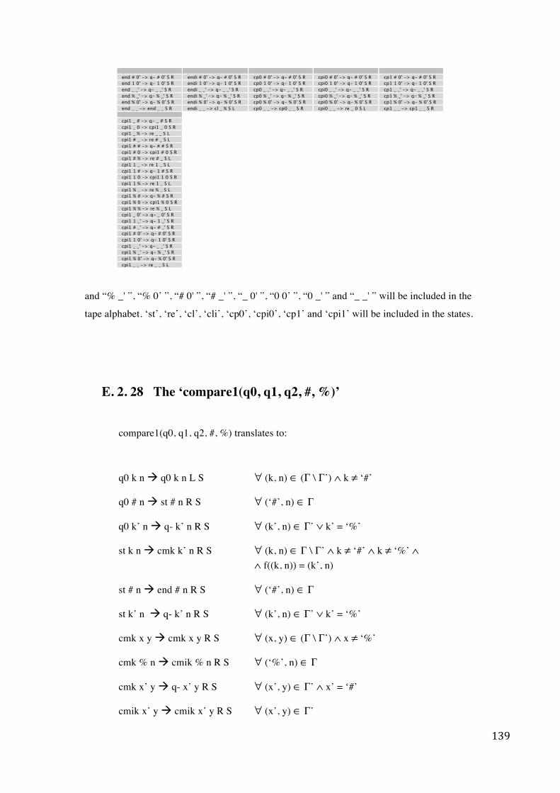
139

end # 0' -> q- # 0' S R endi # 0' -> q- # 0' S R cp0 # 0' -> q- # 0' S R cpi0 # 0' -> q- # 0' S R cp1 # 0' -> q- # 0' S R end 1 0' -> q- 1 0' S R endi 1 0' -> q- 1 0' S R cp0 1 0' -> q- 1 0' S R cpi0 1 0' -> q- 1 0' S R cp1 1 0' -> q- 1 0' S R end _ _' -> q- _ _' S R endi _ _' -> q- _ _' S R cp0 _ _' -> q- _ _' S R cpi0 _ _' -> q- _ _' S R cp1 _ _' -> q- _ _' S R end % _' -> q- % _' S R endi % _' -> q- % _' S R cp0 % _' -> q- % _' S R cpi0 % _' -> q- % _' S R cp1 % _' -> q- % _' S R end % 0' -> q- % 0' S R endi % 0' -> q- % 0' S R cp0 % 0' -> q- % 0' S R cpi0 % 0' -> q- % 0' S R cp1 % 0' -> q- % 0' S R end _ _ -> end _ _ S R endi _ _ -> cl _ % S L cp0 _ _ -> cp0 _ _ S R cpi0 _ _ -> re _ 0 S L cp1 _ _ -> cp1 _ _ S R cpi1 _ # -> q- _ # S R cpi1 _ 0 -> cpi1 _ 0 S R cpi1 _ % -> re _ _ S L cpi1 # _ -> re # _ S L cpi1 # # -> q- # # S R cpi1 # 0 -> cpi1 # 0 S R cpi1 # % -> re # _ S L cpi1 1 _ -> re 1 _ S L cpi1 1 # -> q- 1 # S R cpi1 1 0 -> cpi1 1 0 S R cpi1 1 % -> re 1 _ S L cpi1 % _ -> re % _ S L cpi1 % # -> q- % # S R cpi1 % 0 -> cpi1 % 0 S R cpi1 % % -> re % _ S L cpi1 _ 0' -> q- _ 0' S R cpi1 1 _' -> q- 1 _' S R cpi1 # _' -> q- # _' S R cpi1 # 0' -> q- # 0' S R cpi1 1 0' -> q- 1 0' S R cpi1 _ _' -> q- _ _' S R cpi1 % _' -> q- % _' S R cpi1 % 0' -> q- % 0' S R cpi1 _ _ -> re _ _ S L

and “% _' ”, “% 0’ ”, “# 0' ”, “# _' ”, “_ 0' ”, “0 0’ ”, “0 _' ” and “_ _' ” will be included in the

tape alphabet. ‘st’, ‘re’, ‘cl’, ‘cli’, ‘cp0’, ‘cpi0’, ‘cp1’ and ‘cpi1’ will be included in the states.

E. 2. 28 The ‘compare1(q0, q1, q2, #, %)’

compare1(q0, q1, q2, #, %) translates to:

q0 k n q0 k n L S ∀ (k, n) ∈ (Γ \ Γ’) ∧ k ≠ ‘#’

q0 # n st # n R S ∀ (‘#’, n) ∈ Γ

q0 k’ n q- k’ n R S ∀ (k’, n) ∈ Γ’ ∨ k’ = ‘%’

st k n cmk k’ n R S ∀ (k, n) ∈ Γ \ Γ’ ∧ k ≠ ‘#’ ∧ k ≠ ‘%’ ∧ ∧ f((k, n)) = (k’, n)

st # n end # n R S ∀ (‘#’, n) ∈ Γ

st k’ n q- k’ n R S ∀ (k’, n) ∈ Γ’ ∨ k’ = ‘%’

cmk x y cmk x y R S ∀ (x, y) ∈ (Γ \ Γ’) ∧ x ≠ ‘%’

cmk % n cmik % n R S ∀ (‘%’, n) ∈ Γ

cmk x’ y q- x’ y R S ∀ (x’, y) ∈ Γ’ ∧ x’ = ‘#’

cmik x’ y cmik x’ y R S ∀ (x’, y) ∈ Γ’

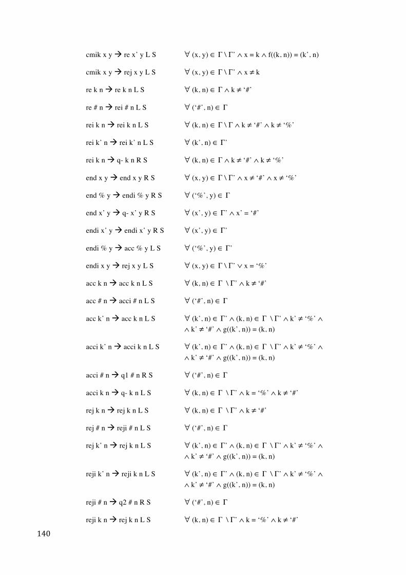
140

cmik x y re x’ y L S ∀ (x, y) ∈ Γ \ Γ’ ∧ x = k ∧ f((k, n)) = (k’, n)

cmik x y rej x y L S ∀ (x, y) ∈ Γ \ Γ’ ∧ x ≠ k

re k n re k n L S ∀ (k, n) ∈ Γ ∧ k ≠ ‘#’

re # n rei # n L S ∀ (‘#’, n) ∈ Γ

rei k n rei k n L S ∀ (k, n) ∈ Γ \ Γ ∧ k ≠ ‘#’ ∧ k ≠ ‘%’

rei k’ n rei k’ n L S ∀ (k’, n) ∈ Γ’

rei k n q- k n R S ∀ (k, n) ∈ Γ ∧ k ≠ ‘#’ ∧ k ≠ ‘%’

end x y end x y R S ∀ (x, y) ∈ Γ \ Γ’ ∧ x ≠ ‘#’ ∧ x ≠ ‘%’

end % y endi % y R S ∀ (‘%’, y) ∈ Γ

end x’ y q- x’ y R S ∀ (x’, y) ∈ Γ’ ∧ x’ = ‘#’

endi x’ y endi x’ y R S ∀ (x’, y) ∈ Γ’

endi % y acc % y L S ∀ (‘%’, y) ∈ Γ’

endi x y rej x y L S ∀ (x, y) ∈ Γ \ Γ’ ∨ x = ‘%’

acc k n acc k n L S ∀ (k, n) ∈ Γ \ Γ’ ∧ k ≠ ‘#’

acc # n acci # n L S ∀ (‘#’, n) ∈ Γ

acc k’ n acc k n L S ∀ (k’, n) ∈ Γ’ ∧ (k, n) ∈ Γ \ Γ’ ∧ k’ ≠ ‘%’ ∧ ∧ k’ ≠ ‘#’ ∧ g((k’, n)) = (k, n)

acci k’ n acci k n L S ∀ (k’, n) ∈ Γ’ ∧ (k, n) ∈ Γ \ Γ’ ∧ k’ ≠ ‘%’ ∧ ∧ k’ ≠ ‘#’ ∧ g((k’, n)) = (k, n)

acci # n q1 # n R S ∀ (‘#’, n) ∈ Γ

acci k n q- k n L S ∀ (k, n) ∈ Γ \ Γ’ ∧ k = ‘%’ ∧ k ≠ ‘#’

rej k n rej k n L S ∀ (k, n) ∈ Γ \ Γ’ ∧ k ≠ ‘#’

rej # n reji # n L S ∀ (‘#’, n) ∈ Γ

rej k’ n rej k n L S ∀ (k’, n) ∈ Γ’ ∧ (k, n) ∈ Γ \ Γ’ ∧ k’ ≠ ‘%’ ∧ ∧ k’ ≠ ‘#’ ∧ g((k’, n)) = (k, n)

reji k’ n reji k n L S ∀ (k’, n) ∈ Γ’ ∧ (k, n) ∈ Γ \ Γ’ ∧ k’ ≠ ‘%’ ∧ ∧ k’ ≠ ‘#’ ∧ g((k’, n)) = (k, n)

reji # n q2 # n R S ∀ (‘#’, n) ∈ Γ

reji k n rej k n L S ∀ (k, n) ∈ Γ \ Γ’ ∧ k = ‘%’ ∧ k ≠ ‘#’

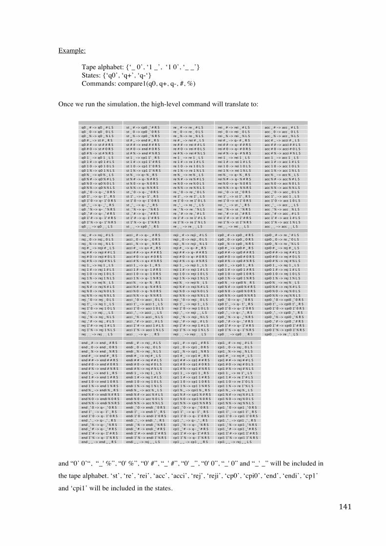
141


Commands: compare1(q0, q+, q-, #, %)


q0 _ # -> q0 _ # L S st _ # -> cp0 _' # R S re _ # -> re _ # L S rei _ # -> rei _ # L S acc _ # -> acc _ # L S q0 _ 0 -> q0 _ 0 L S st _ 0 -> cp0 _' 0 R S re _ 0 -> re _ 0 L S rei _ 0 -> rei _ 0 L S acc _ 0 -> acc _ 0 L S q0 _ % -> q0 _ % L S st _ % -> cp0 _' % R S re _ % -> re _ % L S rei _ % -> rei _ % L S acc _ % -> acc _ % L S q0 # _ -> st # _ R S st # _ -> end # _ R S re # _ -> rei # _ L S rei # _ -> q- # _ R S acc # _ -> acci # _ L S q0 # # -> st # # R S st # # -> end # # R S re # # -> rei # # L S rei # # -> q- # # R S acc # # -> acci # # L S q0 # 0 -> st # 0 R S st # 0 -> end # 0 R S re # 0 -> rei # 0 L S rei # 0 -> q- # 0 R S acc # 0 -> acci # 0 L S q0 # % -> st # % R S st # % -> end # % R S re # % -> rei # % L S rei # % -> q- # % R S acc # % -> acci # % L S q0 1 _ -> q0 1 _ L S st 1 _ -> cp1 1' _ R S re 1 _ -> re 1 _ L S rei 1 _ -> rei 1 _ L S acc 1 _ -> acc 1 _ L S q0 1 # -> q0 1 # L S st 1 # -> cp1 1' # R S re 1 # -> re 1 # L S rei 1 # -> rei 1 # L S acc 1 # -> acc 1 # L S q0 1 0 -> q0 1 0 L S st 1 0 -> cp1 1' 0 R S re 1 0 -> re 1 0 L S rei 1 0 -> rei 1 0 L S acc 1 0 -> acc 1 0 L S q0 1 % -> q0 1 % L S st 1 % -> cp1 1' % R S re 1 % -> re 1 % L S rei 1 % -> rei 1 % L S acc 1 % -> acc 1 % L S q0 % _ -> q0 % _ L S st % _ -> q- % _ R S re % _ -> re % _ L S rei % _ -> q- % _ R S acc % _ -> acc % _ L S q0 % # -> q0 % # L S st % # -> q- % # R S re % # -> re % # L S rei % # -> q- % # R S acc % # -> acc % # L S q0 % 0 -> q0 % 0 L S st % 0 -> q- % 0 R S re % 0 -> re % 0 L S rei % 0 -> q- % 0 R S acc % 0 -> acc % 0 L S q0 % % -> q0 % % L S st % % -> q- % % R S re % % -> re % % L S rei % % -> q- % % R S acc % % -> acc % % L S q0 _' 0 -> q- _' 0 R S st _' 0 -> q- _' 0 R S re _' 0 -> re _' 0 L S rei _' 0 -> st _' 0 R S acc _' 0 -> acc _ 0 L S q0 1' _ -> q- 1' _ R S st 1' _ -> q- 1' _ R S re 1' _ -> re 1' _ L S rei 1' _ -> st 1' _ R S acc 1' _ -> acc 1 _ L S q0 1' 0 -> q- 1' 0 R S st 1' 0 -> q- 1' 0 R S re 1' 0 -> re 1' 0 L S rei 1' 0 -> st 1' 0 R S acc 1' 0 -> acc 1 0 L S q0 _' _ -> q- _' _ R S st _' _ -> q- _' _ R S re _' _ -> re _' _ L S rei _' _ -> st _' _ R S acc _' _ -> acc _ _ L S q0 _' % -> q- _' % R S st _' % -> q- _' % R S re _' % -> re _' % L S rei _' % -> st _' % R S acc _' % -> acc _ % L S q0 _' # -> q- _' # R S st _' # -> q- _' # R S re _' # -> re _' # L S rei _' # -> st _' # R S acc _' # -> acc _ # L S q0 1' # -> q- 1' # R S st 1' # -> q- 1' # R S re 1' # -> re 1' # L S rei 1' # -> st 1' # R S acc 1' # -> acc 1 # L S q0 1' % -> q- 1' % R S st 1' % -> q- 1' % R S re 1' % -> re 1' % L S rei 1' % -> st 1' % R S acc 1' % -> acc 1 % L S q0 _ _ -> q0 _ _ L S st _ _ -> cp0 _' _ R S re _ _ -> re _ _ L S rei _ _ -> rei _ _ L S acc _ _ -> acc _ _ L S rej _ # -> rej _ # L S acci _ # -> q- _ # R S reji _ # -> reji _ # L S cp0 _ # -> cp0 _ # R S cpi0 _ # -> re _' # L S rej _ 0 -> rej _ 0 L S acci _ 0 -> q- _ 0 R S reji _ 0 -> reji _ 0 L S cp0 _ 0 -> cp0 _ 0 R S cpi0 _ 0 -> re _' 0 L S rej _ % -> rej _ % L S acci _ % -> q- _ % R S reji _ % -> reji _ % L S cp0 _ % -> cp0 _ % R S cpi0 _ % -> re _' % L S rej # _ -> reji # _ L S acci # _ -> q+ # _ R S reji # _ -> q- # _ R S cp0 # _ -> cp0 # _ R S cpi0 # _ -> rej # _ L S rej # # -> reji # # L S acci # # -> q+ # # R S reji # # -> q- # # R S cp0 # # -> cp0 # # R S cpi0 # # -> rej # # L S rej # 0 -> reji # 0 L S acci # 0 -> q+ # 0 R S reji # 0 -> q- # 0 R S cp0 # 0 -> cp0 # 0 R S cpi0 # 0 -> rej # 0 L S rej # % -> reji # % L S acci # % -> q+ # % R S reji # % -> q- # % R S cp0 # % -> cp0 # % R S cpi0 # % -> rej # % L S rej 1 _ -> rej 1 _ L S acci 1 _ -> q- 1 _ R S reji 1 _ -> reji 1 _ L S cp0 1 _ -> cp0 1 _ R S cpi0 1 _ -> rej 1 _ L S rej 1 # -> rej 1 # L S acci 1 # -> q- 1 # R S reji 1 # -> reji 1 # L S cp0 1 # -> cp0 1 # R S cpi0 1 # -> rej 1 # L S rej 1 0 -> rej 1 0 L S acci 1 0 -> q- 1 0 R S reji 1 0 -> reji 1 0 L S cp0 1 0 -> cp0 1 0 R S cpi0 1 0 -> rej 1 0 L S rej 1 % -> rej 1 % L S acci 1 % -> q- 1 % R S reji 1 % -> reji 1 % L S cp0 1 % -> cp0 1 % R S cpi0 1 % -> rej 1 % L S rej % _ -> rej % _ L S acci % _ -> q- % _ R S reji % _ -> reji % _ L S cp0 % _ -> cpi0 % _ R S cpi0 % _ -> rej % _ L S rej % # -> rej % # L S acci % # -> q- % # R S reji % # -> reji % # L S cp0 % # -> cpi0 % # R S cpi0 % # -> rej % # L S rej % 0 -> rej % 0 L S acci % 0 -> q- % 0 R S reji % 0 -> reji % 0 L S cp0 % 0 -> cpi0 % 0 R S cpi0 % 0 -> rej % 0 L S rej % % -> rej % % L S acci % % -> q- % % R S reji % % -> reji % % L S cp0 % % -> cpi0 % % R S cpi0 % % -> rej % % L S rej _' 0 -> rej _ 0 L S acci _' 0 -> acci _ 0 L S reji _' 0 -> reji _ 0 L S cp0 _' 0 -> q- _' 0 R S cpi0 _' 0 -> cpi0 _' 0 R S rej 1' _ -> rej 1 _ L S acci 1' _ -> acci 1 _ L S reji 1' _ -> reji 1 _ L S cp0 1' _ -> q- 1' _ R S cpi0 1' _ -> cpi0 1' _ R S rej 1' 0 -> rej 1 0 L S acci 1' 0 -> acci 1 0 L S reji 1' 0 -> reji 1 0 L S cp0 1' 0 -> q- 1' 0 R S cpi0 1' 0 -> cpi0 1' 0 R S rej _' _ -> rej _ _ L S acci _' _ -> acci _ _ L S reji _' _ -> reji _ _ L S cp0 _' _ -> q- _' _ R S cpi0 _' _ -> cpi0 _' _ R S rej _' % -> rej _ % L S acci _' % -> acci _ % L S reji _' % -> reji _ % L S cp0 _' % -> q- _' % R S cpi0 _' % -> cpi0 _' % R S rej _' # -> rej _ # L S acci _' # -> acci _ # L S reji _' # -> reji _ # L S cp0 _' # -> q- _' # R S cpi0 _' # -> cpi0 _' # R S rej 1' # -> rej 1 # L S acci 1' # -> acci 1 # L S reji 1' # -> reji 1 # L S cp0 1' # -> q- 1' # R S cpi0 1' # -> cpi0 1' # R S rej 1' % -> rej 1 % L S acci 1' % -> acci 1 % L S reji 1' % -> reji 1 % L S cp0 1' % -> q- 1' % R S cpi0 1' % -> cpi0 1' % R S rej _ _ -> rej _ _ L S acci _ _ -> q- _ _ R S reji _ _ -> reji _ _ L S cp0 _ _ -> cp0 _ _ R S cpi0 _ _ -> re _' _ L S end _ # -> end _ # R S endi _ # -> rej _ # L S cp1 _ # -> cp1 _ # R S cpi1 _ # -> rej _ # L S end _ 0 -> end _ 0 R S endi _ 0 -> rej _ 0 L S cp1 _ 0 -> cp1 _ 0 R S cpi1 _ 0 -> rej _ 0 L S end _ % -> end _ % R S endi _ % -> rej _ % L S cp1 _ % -> cp1 _ % R S cpi1 _ % -> rej _ % L S end # _ -> end # _ R S endi # _ -> rej # _ L S cp1 # _ -> cp1 # _ R S cpi1 # _ -> rej # _ L S end # # -> end # # R S endi # # -> rej # # L S cp1 # # -> cp1 # # R S cpi1 # # -> rej # # L S end # 0 -> end # 0 R S endi # 0 -> rej # 0 L S cp1 # 0 -> cp1 # 0 R S cpi1 # 0 -> rej # 0 L S end # % -> end # % R S endi # % -> rej # % L S cp1 # % -> cp1 # % R S cpi1 # % -> rej # % L S end 1 _ -> end 1 _ R S endi 1 _ -> rej 1 _ L S cp1 1 _ -> cp1 1 _ R S cpi1 1 _ -> re 1' _ L S end 1 # -> end 1 # R S endi 1 # -> rej 1 # L S cp1 1 # -> cp1 1 # R S cpi1 1 # -> re 1' # L S end 1 0 -> end 1 0 R S endi 1 0 -> rej 1 0 L S cp1 1 0 -> cp1 1 0 R S cpi1 1 0 -> re 1' 0 L S end 1 % -> end 1 % R S endi 1 % -> rej 1 % L S cp1 1 % -> cp1 1 % R S cpi1 1 % -> re 1' % L S end % _ -> endi % _ R S endi % _ -> acc % _ L S cp1 % _ -> cpi1 % _ R S cpi1 % _ -> rej % _ L S end % # -> endi % # R S endi % # -> acc % # L S cp1 % # -> cpi1 % # R S cpi1 % # -> rej % # L S end % 0 -> endi % 0 R S endi % 0 -> acc % 0 L S cp1 % 0 -> cpi1 % 0 R S cpi1 % 0 -> rej % 0 L S end % % -> endi % % R S endi % % -> acc % % L S cp1 % % -> cpi1 % % R S cpi1 % % -> rej % % L S end _' 0 -> q- _' 0 R S endi _' 0 -> endi _' 0 R S cp1 _' 0 -> q- _' 0 R S cpi1 _' 0 -> cpi1 _' 0 R S end 1' _ -> q- 1' _ R S endi 1' _ -> endi 1' _ R S cp1 1' _ -> q- 1' _ R S cpi1 1' _ -> cpi1 1' _ R S end 1' 0 -> q- 1' 0 R S endi 1' 0 -> endi 1' 0 R S cp1 1' 0 -> q- 1' 0 R S cpi1 1' 0 -> cpi1 1' 0 R S end _' _ -> q- _' _ R S endi _' _ -> endi _' _ R S cp1 _' _ -> q- _' _ R S cpi1 _' _ -> cpi1 _' _ R S end _' % -> q- _' % R S endi _' % -> endi _' % R S cp1 _' % -> q- _' % R S cpi1 _' % -> cpi1 _' % R S end _' # -> q- _' # R S endi _' # -> endi _' # R S cp1 _' # -> q- _' # R S cpi1 _' # -> cpi1 _' # R S end 1' # -> q- 1' # R S endi 1' # -> endi 1' # R S cp1 1' # -> q- 1' # R S cpi1 1' # -> cpi1 1' # R S end 1' % -> q- 1' % R S endi 1' % -> endi 1' % R S cp1 1' % -> q- 1' % R S cpi1 1' % -> cpi1 1' % R S end _ _ -> end _ _ R S endi _ _ -> rej _ _ L S cp1 _ _ -> cp1 _ _ R S cpi1 _ _ -> rej _ _ L S

and “0’ 0’“, “_' %”, “0' %”, “0' #”, “_' #”, “0' _”, “0' 0”, “_' 0” and “_' _” will be included in

the tape alphabet. ‘st’, ‘re’, ‘rei’, ‘acc’, ‘acci’, ‘rej’, ‘reji’, ‘cp0’, ‘cpi0’, ‘end’, ‘endi’, ‘cp1’

and ‘cpi1’ will be included in the states.

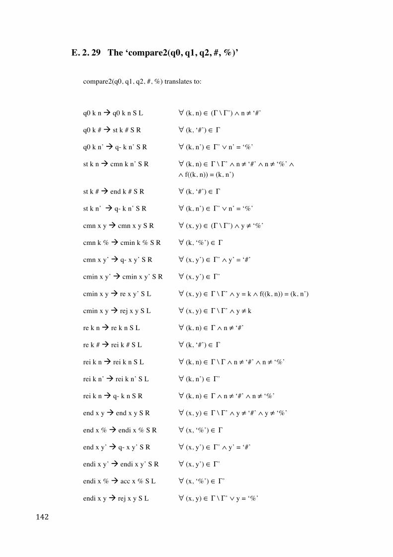
142

E. 2. 29 The ‘compare2(q0, q1, q2, #, %)’

compare2(q0, q1, q2, #, %) translates to:

q0 k n q0 k n S L ∀ (k, n) ∈ (Γ \ Γ’) ∧ n ≠ ‘#’

q0 k # st k # S R ∀ (k, ‘#’) ∈ Γ

q0 k n’ q- k n’ S R ∀ (k, n’) ∈ Γ’ ∨ n’ = ‘%’

st k n cmn k n’ S R ∀ (k, n) ∈ Γ \ Γ’ ∧ n ≠ ‘#’ ∧ n ≠ ‘%’ ∧ ∧ f((k, n)) = (k, n’)

st k # end k # S R ∀ (k, ‘#’) ∈ Γ

st k n’ q- k n’ S R ∀ (k, n’) ∈ Γ’ ∨ n’ = ‘%’

cmn x y cmn x y S R ∀ (x, y) ∈ (Γ \ Γ’) ∧ y ≠ ‘%’

cmn k % cmin k % S R ∀ (k, ‘%’) ∈ Γ

cmn x y’ q- x y’ S R ∀ (x, y’) ∈ Γ’ ∧ y’ = ‘#’

cmin x y’ cmin x y’ S R ∀ (x, y’) ∈ Γ’

cmin x y re x y’ S L ∀ (x, y) ∈ Γ \ Γ’ ∧ y = k ∧ f((k, n)) = (k, n’)

cmin x y rej x y S L ∀ (x, y) ∈ Γ \ Γ’ ∧ y ≠ k

re k n re k n S L ∀ (k, n) ∈ Γ ∧ n ≠ ‘#’

re k # rei k # S L ∀ (k, ‘#’) ∈ Γ

rei k n rei k n S L ∀ (k, n) ∈ Γ \ Γ ∧ n ≠ ‘#’ ∧ n ≠ ‘%’

rei k n’ rei k n’ S L ∀ (k, n’) ∈ Γ’

rei k n q- k n S R ∀ (k, n) ∈ Γ ∧ n ≠ ‘#’ ∧ n ≠ ‘%’

end x y end x y S R ∀ (x, y) ∈ Γ \ Γ’ ∧ y ≠ ‘#’ ∧ y ≠ ‘%’

end x % endi x % S R ∀ (x, ‘%’) ∈ Γ

end x y’ q- x y’ S R ∀ (x, y’) ∈ Γ’ ∧ y’ = ‘#’

endi x y’ endi x y’ S R ∀ (x, y’) ∈ Γ’

endi x % acc x % S L ∀ (x, ‘%’) ∈ Γ’

endi x y rej x y S L ∀ (x, y) ∈ Γ \ Γ’ ∨ y = ‘%’

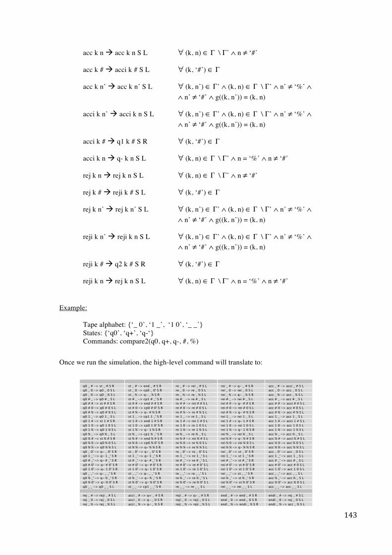
143

acc k n acc k n S L ∀ (k, n) ∈ Γ \ Γ’ ∧ n ≠ ‘#’

acc k # acci k # S L ∀ (k, ‘#’) ∈ Γ

acc k n’ acc k n’ S L ∀ (k, n’) ∈ Γ’ ∧ (k, n) ∈ Γ \ Γ’ ∧ n’ ≠ ‘%’ ∧ ∧ n’ ≠ ‘#’ ∧ g((k, n’)) = (k, n)

acci k n’ acci k n S L ∀ (k, n’) ∈ Γ’ ∧ (k, n) ∈ Γ \ Γ’ ∧ n’ ≠ ‘%’ ∧ ∧ n’ ≠ ‘#’ ∧ g((k, n’)) = (k, n)

acci k # q1 k # S R ∀ (k, ‘#’) ∈ Γ

acci k n q- k n S L ∀ (k, n) ∈ Γ \ Γ’ ∧ n = ‘%’ ∧ n ≠ ‘#’

rej k n rej k n S L ∀ (k, n) ∈ Γ \ Γ’ ∧ n ≠ ‘#’

rej k # reji k # S L ∀ (k, ‘#’) ∈ Γ

rej k n’ rej k n’ S L ∀ (k, n’) ∈ Γ’ ∧ (k, n) ∈ Γ \ Γ’ ∧ n’ ≠ ‘%’ ∧ ∧ n’ ≠ ‘#’ ∧ g((k, n’)) = (k, n)

reji k n’ reji k n S L ∀ (k, n’) ∈ Γ’ ∧ (k, n) ∈ Γ \ Γ’ ∧ n’ ≠ ‘%’ ∧ ∧ n’ ≠ ‘#’ ∧ g((k, n’)) = (k, n)

reji k # q2 k # S R ∀ (k, ‘#’) ∈ Γ

reji k n rej k n S L ∀ (k, n) ∈ Γ \ Γ’ ∧ n = ‘%’ ∧ n ≠ ‘#’


Commands: compare2(q0, q+, q-, #, %)


q0 _ # -> st _ # S R st _ # -> end _ # S R re _ # -> rei _ # S L rei _ # -> q- _ # S R acc _ # -> acci _ # S L q0 _ 0 -> q0 _ 0 S L st _ 0 -> cp0 _ 0' S R re _ 0 -> re _ 0 S L rei _ 0 -> rei _ 0 S L acc _ 0 -> acc _ 0 S L q0 _ % -> q0 _ % S L st _ % -> q- _ % S R re _ % -> re _ % S L rei _ % -> q- _ % S R acc _ % -> acc _ % S L q0 # _ -> q0 # _ S L st # _ -> cp1 # _' S R re # _ -> re # _ S L rei # _ -> rei # _ S L acc # _ -> acc # _ S L q0 # # -> st # # S R st # # -> end # # S R re # # -> rei # # S L rei # # -> q- # # S R acc # # -> acci # # S L q0 # 0 -> q0 # 0 S L st # 0 -> cp0 # 0' S R re # 0 -> re # 0 S L rei # 0 -> rei # 0 S L acc # 0 -> acc # 0 S L q0 # % -> q0 # % S L st # % -> q- # % S R re # % -> re # % S L rei # % -> q- # % S R acc # % -> acc # % S L q0 1 _ -> q0 1 _ S L st 1 _ -> cp1 1 _' S R re 1 _ -> re 1 _ S L rei 1 _ -> rei 1 _ S L acc 1 _ -> acc 1 _ S L q0 1 # -> st 1 # S R st 1 # -> end 1 # S R re 1 # -> rei 1 # S L rei 1 # -> q- 1 # S R acc 1 # -> acci 1 # S L q0 1 0 -> q0 1 0 S L st 1 0 -> cp0 1 0' S R re 1 0 -> re 1 0 S L rei 1 0 -> rei 1 0 S L acc 1 0 -> acc 1 0 S L q0 1 % -> q0 1 % S L st 1 % -> q- 1 % S R re 1 % -> re 1 % S L rei 1 % -> q- 1 % S R acc 1 % -> acc 1 % S L q0 % _ -> q0 % _ S L st % _ -> cp1 % _' S R re % _ -> re % _ S L rei % _ -> rei % _ S L acc % _ -> acc % _ S L q0 % # -> st % # S R st % # -> end % # S R re % # -> rei % # S L rei % # -> q- % # S R acc % # -> acci % # S L q0 % 0 -> q0 % 0 S L st % 0 -> cp0 % 0' S R re % 0 -> re % 0 S L rei % 0 -> rei % 0 S L acc % 0 -> acc % 0 S L q0 % % -> q0 % % S L st % % -> q- % % S R re % % -> re % % S L rei % % -> q- % % S R acc % % -> acc % % S L q0 _ 0' -> q- _ 0' S R st _ 0' -> q- _ 0' S R re _ 0' -> re _ 0' S L rei _ 0' -> st _ 0' S R acc _ 0' -> acc _ 0 S L q0 1 _' -> q- 1 _' S R st 1 _' -> q- 1 _' S R re 1 _' -> re 1 _' S L rei 1 _' -> st 1 _' S R acc 1 _' -> acc 1 _ S L q0 # _' -> q- # _' S R st # _' -> q- # _' S R re # _' -> re # _' S L rei # _' -> st # _' S R acc # _' -> acc # _ S L q0 # 0' -> q- # 0' S R st # 0' -> q- # 0' S R re # 0' -> re # 0' S L rei # 0' -> st # 0' S R acc # 0' -> acc # 0 S L q0 1 0' -> q- 1 0' S R st 1 0' -> q- 1 0' S R re 1 0' -> re 1 0' S L rei 1 0' -> st 1 0' S R acc 1 0' -> acc 1 0 S L q0 _ _' -> q- _ _' S R st _ _' -> q- _ _' S R re _ _' -> re _ _' S L rei _ _' -> st _ _' S R acc _ _' -> acc _ _ S L q0 % _' -> q- % _' S R st % _' -> q- % _' S R re % _' -> re % _' S L rei % _' -> st % _' S R acc % _' -> acc % _ S L q0 % 0' -> q- % 0' S R st % 0' -> q- % 0' S R re % 0' -> re % 0' S L rei % 0' -> st % 0' S R acc % 0' -> acc % 0 S L q0 _ _ -> q0 _ _ S L st _ _ -> cp1 _ _' S R re _ _ -> re _ _ S L rei _ _ -> rei _ _ S L acc _ _ -> acc _ _ S L rej _ # -> reji _ # S L acci _ # -> q+ _ # S R reji _ # -> q- _ # S R end _ # -> end _ # S R endi _ # -> rej _ # S L rej _ 0 -> rej _ 0 S L acci _ 0 -> q- _ 0 S R reji _ 0 -> reji _ 0 S L end _ 0 -> end _ 0 S R endi _ 0 -> rej _ 0 S L rej _ % -> rej _ % S L acci _ % -> q- _ % S R reji _ % -> reji _ % S L end _ % -> endi _ % S R endi _ % -> acc _ % S L

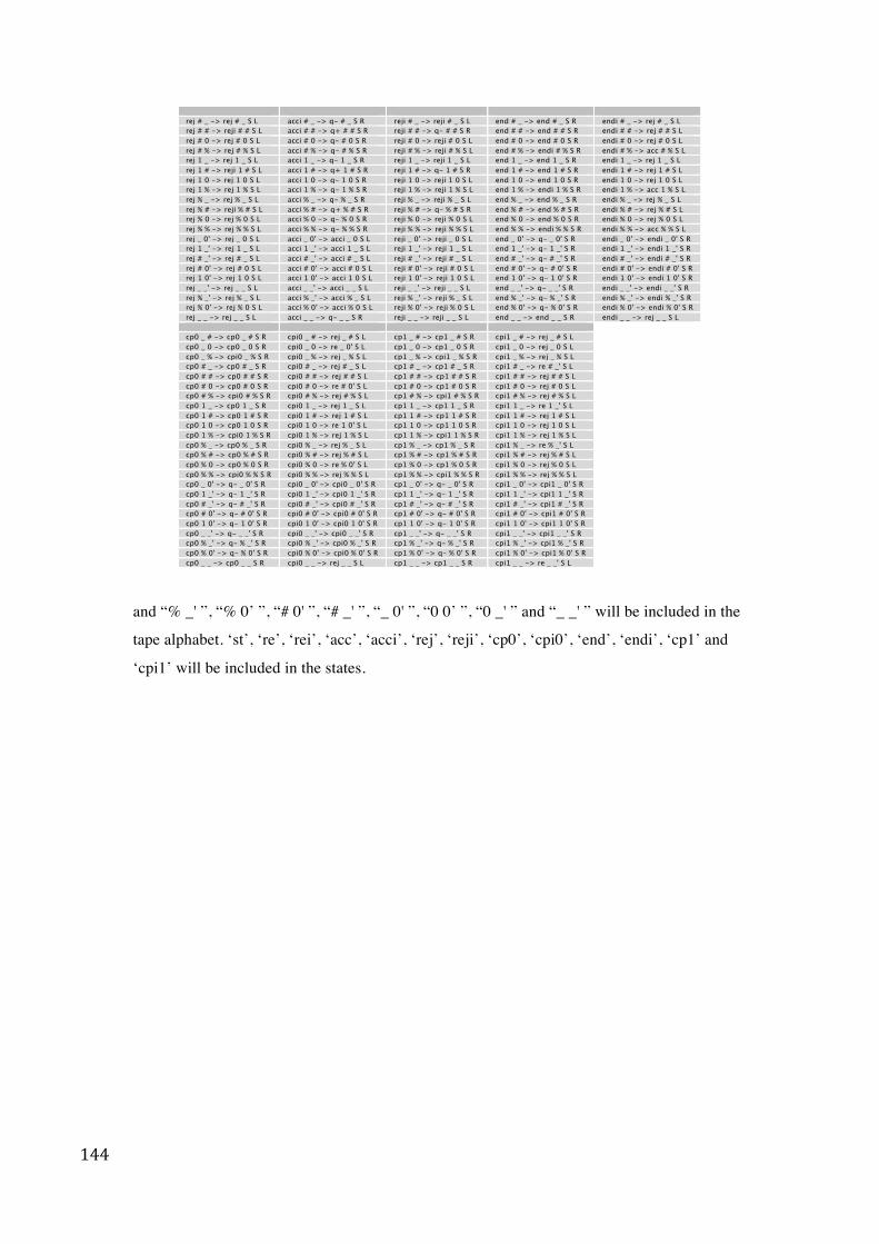
144

rej # _ -> rej # _ S L acci # _ -> q- # _ S R reji # _ -> reji # _ S L end # _ -> end # _ S R endi # _ -> rej # _ S L rej # # -> reji # # S L acci # # -> q+ # # S R reji # # -> q- # # S R end # # -> end # # S R endi # # -> rej # # S L rej # 0 -> rej # 0 S L acci # 0 -> q- # 0 S R reji # 0 -> reji # 0 S L end # 0 -> end # 0 S R endi # 0 -> rej # 0 S L rej # % -> rej # % S L acci # % -> q- # % S R reji # % -> reji # % S L end # % -> endi # % S R endi # % -> acc # % S L rej 1 _ -> rej 1 _ S L acci 1 _ -> q- 1 _ S R reji 1 _ -> reji 1 _ S L end 1 _ -> end 1 _ S R endi 1 _ -> rej 1 _ S L rej 1 # -> reji 1 # S L acci 1 # -> q+ 1 # S R reji 1 # -> q- 1 # S R end 1 # -> end 1 # S R endi 1 # -> rej 1 # S L rej 1 0 -> rej 1 0 S L acci 1 0 -> q- 1 0 S R reji 1 0 -> reji 1 0 S L end 1 0 -> end 1 0 S R endi 1 0 -> rej 1 0 S L rej 1 % -> rej 1 % S L acci 1 % -> q- 1 % S R reji 1 % -> reji 1 % S L end 1 % -> endi 1 % S R endi 1 % -> acc 1 % S L rej % _ -> rej % _ S L acci % _ -> q- % _ S R reji % _ -> reji % _ S L end % _ -> end % _ S R endi % _ -> rej % _ S L rej % # -> reji % # S L acci % # -> q+ % # S R reji % # -> q- % # S R end % # -> end % # S R endi % # -> rej % # S L rej % 0 -> rej % 0 S L acci % 0 -> q- % 0 S R reji % 0 -> reji % 0 S L end % 0 -> end % 0 S R endi % 0 -> rej % 0 S L rej % % -> rej % % S L acci % % -> q- % % S R reji % % -> reji % % S L end % % -> endi % % S R endi % % -> acc % % S L rej _ 0' -> rej _ 0 S L acci _ 0' -> acci _ 0 S L reji _ 0' -> reji _ 0 S L end _ 0' -> q- _ 0' S R endi _ 0' -> endi _ 0' S R rej 1 _' -> rej 1 _ S L acci 1 _' -> acci 1 _ S L reji 1 _' -> reji 1 _ S L end 1 _' -> q- 1 _' S R endi 1 _' -> endi 1 _' S R rej # _' -> rej # _ S L acci # _' -> acci # _ S L reji # _' -> reji # _ S L end # _' -> q- # _' S R endi # _' -> endi # _' S R rej # 0' -> rej # 0 S L acci # 0' -> acci # 0 S L reji # 0' -> reji # 0 S L end # 0' -> q- # 0' S R endi # 0' -> endi # 0' S R rej 1 0' -> rej 1 0 S L acci 1 0' -> acci 1 0 S L reji 1 0' -> reji 1 0 S L end 1 0' -> q- 1 0' S R endi 1 0' -> endi 1 0' S R rej _ _' -> rej _ _ S L acci _ _' -> acci _ _ S L reji _ _' -> reji _ _ S L end _ _' -> q- _ _' S R endi _ _' -> endi _ _' S R rej % _' -> rej % _ S L acci % _' -> acci % _ S L reji % _' -> reji % _ S L end % _' -> q- % _' S R endi % _' -> endi % _' S R rej % 0' -> rej % 0 S L acci % 0' -> acci % 0 S L reji % 0' -> reji % 0 S L end % 0' -> q- % 0' S R endi % 0' -> endi % 0' S R rej _ _ -> rej _ _ S L acci _ _ -> q- _ _ S R reji _ _ -> reji _ _ S L end _ _ -> end _ _ S R endi _ _ -> rej _ _ S L cp0 _ # -> cp0 _ # S R cpi0 _ # -> rej _ # S L cp1 _ # -> cp1 _ # S R cpi1 _ # -> rej _ # S L cp0 _ 0 -> cp0 _ 0 S R cpi0 _ 0 -> re _ 0' S L cp1 _ 0 -> cp1 _ 0 S R cpi1 _ 0 -> rej _ 0 S L cp0 _ % -> cpi0 _ % S R cpi0 _ % -> rej _ % S L cp1 _ % -> cpi1 _ % S R cpi1 _ % -> rej _ % S L cp0 # _ -> cp0 # _ S R cpi0 # _ -> rej # _ S L cp1 # _ -> cp1 # _ S R cpi1 # _ -> re # _' S L cp0 # # -> cp0 # # S R cpi0 # # -> rej # # S L cp1 # # -> cp1 # # S R cpi1 # # -> rej # # S L cp0 # 0 -> cp0 # 0 S R cpi0 # 0 -> re # 0' S L cp1 # 0 -> cp1 # 0 S R cpi1 # 0 -> rej # 0 S L cp0 # % -> cpi0 # % S R cpi0 # % -> rej # % S L cp1 # % -> cpi1 # % S R cpi1 # % -> rej # % S L cp0 1 _ -> cp0 1 _ S R cpi0 1 _ -> rej 1 _ S L cp1 1 _ -> cp1 1 _ S R cpi1 1 _ -> re 1 _' S L cp0 1 # -> cp0 1 # S R cpi0 1 # -> rej 1 # S L cp1 1 # -> cp1 1 # S R cpi1 1 # -> rej 1 # S L cp0 1 0 -> cp0 1 0 S R cpi0 1 0 -> re 1 0' S L cp1 1 0 -> cp1 1 0 S R cpi1 1 0 -> rej 1 0 S L cp0 1 % -> cpi0 1 % S R cpi0 1 % -> rej 1 % S L cp1 1 % -> cpi1 1 % S R cpi1 1 % -> rej 1 % S L cp0 % _ -> cp0 % _ S R cpi0 % _ -> rej % _ S L cp1 % _ -> cp1 % _ S R cpi1 % _ -> re % _' S L cp0 % # -> cp0 % # S R cpi0 % # -> rej % # S L cp1 % # -> cp1 % # S R cpi1 % # -> rej % # S L cp0 % 0 -> cp0 % 0 S R cpi0 % 0 -> re % 0' S L cp1 % 0 -> cp1 % 0 S R cpi1 % 0 -> rej % 0 S L cp0 % % -> cpi0 % % S R cpi0 % % -> rej % % S L cp1 % % -> cpi1 % % S R cpi1 % % -> rej % % S L cp0 _ 0' -> q- _ 0' S R cpi0 _ 0' -> cpi0 _ 0' S R cp1 _ 0' -> q- _ 0' S R cpi1 _ 0' -> cpi1 _ 0' S R cp0 1 _' -> q- 1 _' S R cpi0 1 _' -> cpi0 1 _' S R cp1 1 _' -> q- 1 _' S R cpi1 1 _' -> cpi1 1 _' S R cp0 # _' -> q- # _' S R cpi0 # _' -> cpi0 # _' S R cp1 # _' -> q- # _' S R cpi1 # _' -> cpi1 # _' S R cp0 # 0' -> q- # 0' S R cpi0 # 0' -> cpi0 # 0' S R cp1 # 0' -> q- # 0' S R cpi1 # 0' -> cpi1 # 0' S R cp0 1 0' -> q- 1 0' S R cpi0 1 0' -> cpi0 1 0' S R cp1 1 0' -> q- 1 0' S R cpi1 1 0' -> cpi1 1 0' S R cp0 _ _' -> q- _ _' S R cpi0 _ _' -> cpi0 _ _' S R cp1 _ _' -> q- _ _' S R cpi1 _ _' -> cpi1 _ _' S R cp0 % _' -> q- % _' S R cpi0 % _' -> cpi0 % _' S R cp1 % _' -> q- % _' S R cpi1 % _' -> cpi1 % _' S R cp0 % 0' -> q- % 0' S R cpi0 % 0' -> cpi0 % 0' S R cp1 % 0' -> q- % 0' S R cpi1 % 0' -> cpi1 % 0' S R cp0 _ _ -> cp0 _ _ S R cpi0 _ _ -> rej _ _ S L cp1 _ _ -> cp1 _ _ S R cpi1 _ _ -> re _ _' S L

and “% _' ”, “% 0’ ”, “# 0' ”, “# _' ”, “_ 0' ”, “0 0’ ”, “0 _' ” and “_ _' ” will be included in the

tape alphabet. ‘st’, ‘re’, ‘rei’, ‘acc’, ‘acci’, ‘rej’, ‘reji’, ‘cp0’, ‘cpi0’, ‘end’, ‘endi’, ‘cp1’ and

‘cpi1’ will be included in the states.

145

Appendix F: In the CD

The CD attached to this report contains 2 folders:

• Program

o TuringSlashPython.py – the simulator o onInput.py – a class that is imported by TuringSlashPython that handles

XML o folder ‘files’ – images needed for the simulator and the how-to file

• Evaluation

o Tutorial.pdf – the tutorial used in the evaluation o Folder ‘files’ – the files used in the tutorial

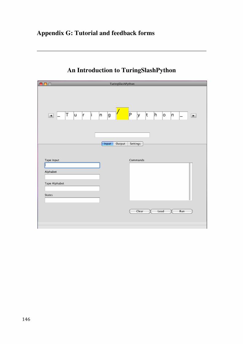
146

Appendix G: Tutorial and feedback forms

An Introduction to TuringSlashPython

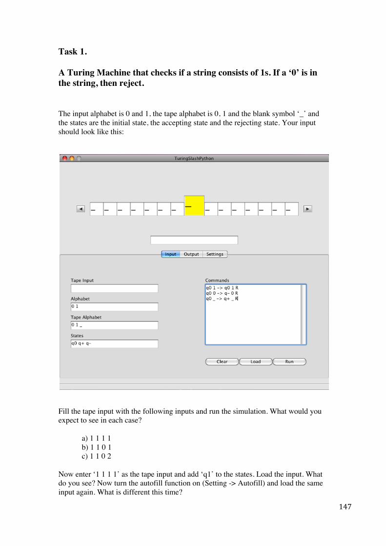
147

Task 1. A Turing Machine that checks if a string consists of 1s. If a ‘0’ is in the string, then reject. The input alphabet is 0 and 1, the tape alphabet is 0, 1 and the blank symbol ‘_’ and the states are the initial state, the accepting state and the rejecting state. Your input should look like this:

Fill the tape input with the following inputs and run the simulation. What would you expect to see in each case?

a) 1 1 1 1 b) 1 1 0 1 c) 1 1 0 2

Now enter ‘1 1 1 1’ as the tape input and add ‘q1’ to the states. Load the input. What do you see? Now turn the autofill function on (Setting -> Autofill) and load the same input again. What is different this time?

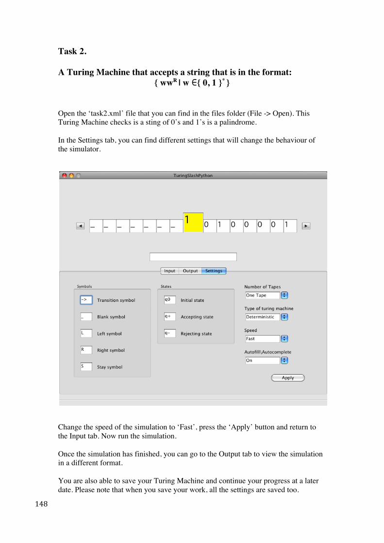
148

Task 2. A Turing Machine that accepts a string that is in the format:

{ wwR | w ∈{ 0, 1 }* }

Open the ‘task2.xml’ file that you can find in the files folder (File -> Open). This Turing Machine checks is a sting of 0’s and 1’s is a palindrome. In the Settings tab, you can find different settings that will change the behaviour of the simulator.

Change the speed of the simulation to ‘Fast’, press the ‘Apply’ button and return to the Input tab. Now run the simulation. Once the simulation has finished, you can go to the Output tab to view the simulation in a different format. You are also able to save your Turing Machine and continue your progress at a later date. Please note that when you save your work, all the settings are saved too.

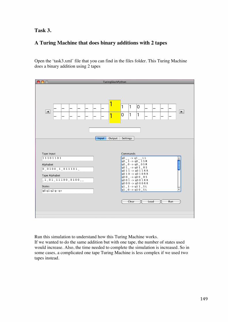
149

Task 3. A Turing Machine that does binary additions with 2 tapes Open the ‘task3.xml’ file that you can find in the files folder. This Turing Machine does a binary addition using 2 tapes

Run this simulation to understand how this Turing Machine works. If we wanted to do the same addition but with one tape, the number of states used would increase. Also, the time needed to complete the simulation is increased. So in some cases, a complicated one tape Turing Machine is less complex if we used two tapes instead.

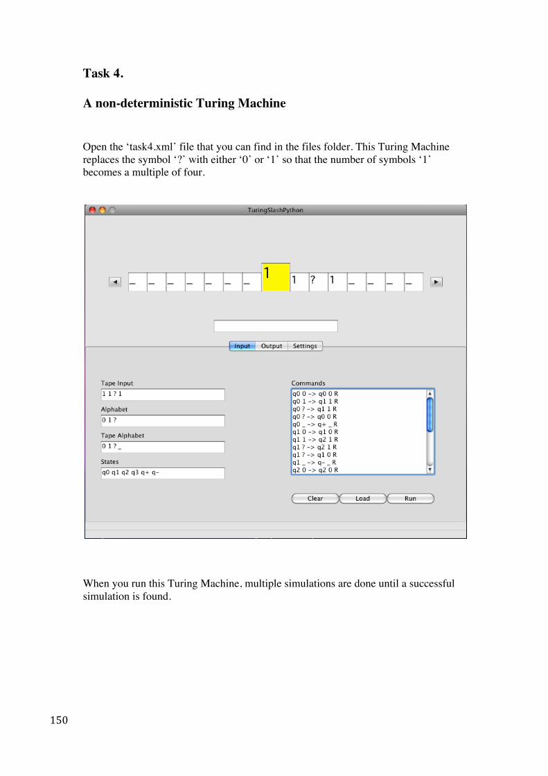
150

Task 4. A non-deterministic Turing Machine Open the ‘task4.xml’ file that you can find in the files folder. This Turing Machine replaces the symbol ‘?’ with either ‘0’ or ‘1’ so that the number of symbols ‘1’ becomes a multiple of four.

When you run this Turing Machine, multiple simulations are done until a successful simulation is found.

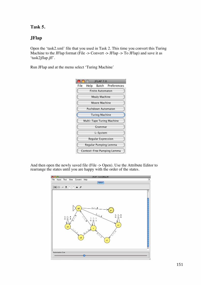
151

Task 5. JFlap Open the ‘task2.xml’ file that you used in Task 2. This time you convert this Turing Machine to the JFlap format (File -> Convert -> JFlap -> To JFlap) and save it as ‘task2jflap.jff’. Run JFlap and at the menu select ‘Turing Machine’

And then open the newly saved file (File -> Open). Use the Attribute Editor to rearrange the states until you are happy with the order of the states.

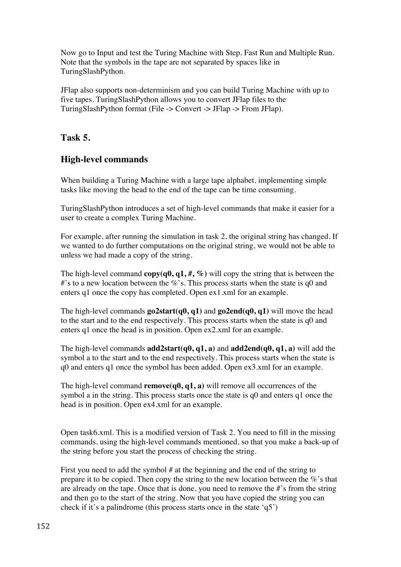
152

Now go to Input and test the Turing Machine with Step, Fast Run and Multiple Run. Note that the symbols in the tape are not separated by spaces like in TuringSlashPython. JFlap also supports non-determinism and you can build Turing Machine with up to five tapes. TuringSlashPython allows you to convert JFlap files to the TuringSlashPython format (File -> Convert -> JFlap -> From JFlap). Task 5. High-level commands When building a Turing Machine with a large tape alphabet, implementing simple tasks like moving the head to the end of the tape can be time consuming. TuringSlashPython introduces a set of high-level commands that make it easier for a user to create a complex Turing Machine. For example, after running the simulation in task 2, the original string has changed. If we wanted to do further computations on the original string, we would not be able to unless we had made a copy of the string. The high-level command copy(q0, q1, #, %) will copy the string that is between the #’s to a new location between the %’s. This process starts when the state is q0 and enters q1 once the copy has completed. Open ex1.xml for an example. The high-level commands go2start(q0, q1) and go2end(q0, q1) will move the head to the start and to the end respectively. This process starts when the state is q0 and enters q1 once the head is in position. Open ex2.xml for an example. The high-level commands add2start(q0, q1, a) and add2end(q0, q1, a) will add the symbol a to the start and to the end respectively. This process starts when the state is q0 and enters q1 once the symbol has been added. Open ex3.xml for an example. The high-level command remove(q0, q1, a) will remove all occurrences of the symbol a in the string. This process starts once the state is q0 and enters q1 once the head is in position. Open ex4.xml for an example. Open task6.xml. This is a modified version of Task 2. You need to fill in the missing commands, using the high-level commands mentioned, so that you make a back-up of the string before you start the process of checking the string. First you need to add the symbol # at the beginning and the end of the string to prepare it to be copied. Then copy the string to the new location between the %’s that are already on the tape. Once that is done, you need to remove the #’s from the string and then go to the start of the string. Now that you have copied the string you can check if it’s a palindrome (this process starts once in the state ‘q5’)

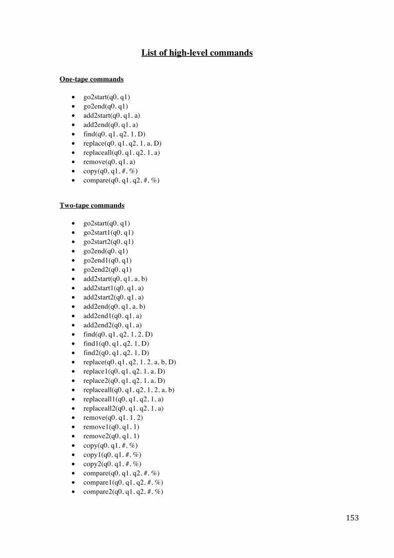
153

List of high-level commands

One-tape commands

• go2start(q0, q1) • go2end(q0, q1) • add2start(q0, q1, a) • add2end(q0, q1, a) • find(q0, q1, q2, 1, D) • replace(q0, q1, q2, 1, a, D) • replaceall(q0, q1, q2, 1, a) • remove(q0, q1, a) • copy(q0, q1, #, %) • compare(q0, q1, q2, #, %)

Two-tape commands

• go2start(q0, q1) • go2start1(q0, q1) • go2start2(q0, q1) • go2end(q0, q1) • go2end1(q0, q1) • go2end2(q0, q1) • add2start(q0, q1, a, b) • add2start1(q0, q1, a) • add2start2(q0, q1, a) • add2end(q0, q1, a, b) • add2end1(q0, q1, a) • add2end2(q0, q1, a) • find(q0, q1, q2, 1, 2, D) • find1(q0, q1, q2, 1, D) • find2(q0, q1, q2, 1, D) • replace(q0, q1, q2, 1, 2, a, b, D) • replace1(q0, q1, q2, 1, a, D) • replace2(q0, q1, q2, 1, a, D) • replaceall(q0, q1, q2, 1, 2, a, b) • replaceall1(q0, q1, q2, 1, a) • replaceall2(q0, q1, q2, 1, a) • remove(q0, q1, 1, 2) • remove1(q0, q1, 1) • remove2(q0, q1, 1) • copy(q0, q1, #, %) • copy1(q0, q1, #, %) • copy2(q0, q1, #, %) • compare(q0, q1, q2, #, %) • compare1(q0, q1, q2, #, %) • compare2(q0, q1, q2, #, %)

Documents

A Turing Machine simulator for academic uses … · Conversion from and to the JFlap Turing Machine format. 1. 4 Extensions Possible extensions are: I. Two-tape features. ! 2! II