1

A Unified Asymptotic Analysis of Area

Spectral Efficiency in Ultradense Cellular

Networks

Ahmad AlAmmouri, Jeffrey G. Andrews, and Francois Baccelli

Abstract

This paper studies the asymptotic properties of area spectral efficiency (ASE) of a downlink cellular

network in the limit of very dense base station (BS) and user densities. This asymptotic analysis relies

on three assumptions: (1) interference is treated as noise; (2) the BS locations are drawn from a Poisson

point process; (3) the path loss function is bounded above satisfying mild regularity conditions. We

consider three possible definitions of the ASE, all of which give units of bits per second per unit area.

When there is no constraint on the minimum operational SINR and instantaneous full channel state

information is available at the transmitter, the ASE is proven to saturate to a constant, which we derive

in closed form. For the other two ASE definitions, wherein either a minimum SINR is enforced or full

CSI is not available, the ASE is instead shown to collapse to zero at high BS density. We provide several

familiar case studies for the class of considered path loss models, and demonstrate that our results cover

most previous models and results on ultradense networks as special cases.

I. INTRODUCTION

The reuse of spectrum across space, called frequency or spatial reuse, is historically the

most important attribute of terrestrial wireless networks. Installing new cellular or wireless LAN

infrastructure is expected to generate spatial reuse, whereby the time and frequency resources can

be reused across smaller spatial scales. A major question within this context is whether this will

indefinitely bring higher overall data throughputs in the network. The ASE, defined as the sum

of the maximum data rate per unit area per unit bandwidth [1], has historically increased about

The authors are with the Wireless Networking and Communications Group (WNCG), The University of Texas at Austin, Austin,

TX 78701 USA. (Email: {alammouri@utexas.edu, jandrews@ece.utexas.edu, francois.baccelli@austin.utexas.edu}). Last revised

December 20, 2017.

2

linearly with the number of BSs: doubling the number of BSs about doubles the sum throughput

the network supports in a given area. This has often been referred to as “cell splitting gain”

or “densification gain” and has been the most significant driver in increased wireless data rates

over the last few decades [2], [3], and is expected to continue to drive gains for the foreseeable

future as well [4], [5]. The aim of the present paper is to clarify what can in fact be expected

in terms of ASE under densification. This is done by the definition of a general model allowing

one to study the asymptotic behavior of ASE under broad conditions.

A. Related Work

The study of dense wireless network capacity has a rich history, in particular for the case of

ad hoc multihop networks. The seminal result of Gupta and Kumar [6] showed that the transport

capacity of an infrastructure-less network increases with the number of nodes n roughly as√n,

assuming a given node wishes to transmit with a randomly selected other node. Many subsequent

results extended this “scaling law” approach to a wide variety of models and communication

techniques, well summarized in [7]. A main intuition from these results is that the best network-

wide throughput scaling is achieved by short-range local communication coupled with multi-

hopping towards the intended receiver, a form of spatial reuse. A key subsequent paper showed

that this square-root scaling is a fundamental property of the electromagnetic propagation [8],

thus attempts to improve the scaling law through exotic communication strategies would be

futile.

To obtain mathematically tractable results on wireless network performance without resorting

to scaling laws, stochastic geometry [9]–[12] has emerged as a key toolset, in particular for

deriving the SINR distribution and related metrics, as achieved for ad hoc networks in [13],

[14]. One of the key conclusions of early stochastic geometry results for cellular networks such

as [15], [16] was that the SINR distribution is insensitive to the BS density, once the network is

interference-limited. This indicated that the ASE should increase linearly with the BS density:

an encouraging result. Both [15], [16], as well as most prior and subsequent literature including

the aforementioned scaling laws results, use a standard power-law path loss function of the form

L(r) = c0r−η, where r is the distance, c0 = L(1) is a constant, and η > 2 is the path loss

exponent.

However, other more recent works have shown that when adopting more realistic bounded

path loss models, different and much more pessimistic trends can be derived or observed for ASE

3

under densification [17]–[22]. The current situation can be summarized by saying that depending

on the path loss model and the ASE definition, one finds in the literature the whole spectrum

of asymptotic behaviors for ASE ranging from linear growth to collapse.

It is well understood that the pole at the origin of the standard power law model creates a

scale free cellular SIR which is the basis for the linear ASE growth alluded to above. It is also

well understood that this standard power-law path loss model has important shortcomings in the

context of dense networks: first, it does not accurately model received powers for short distances,

and second, it is intractable for line-of-sight propagation, i.e., η = 2. The more realistic bounded

path loss models alluded to above, which are the main focus of the present paper, are hence

much more natural within the context of ultra-densification. We describe several of these refined

models and results in more detail in Sect. V, and show, through a few typical examples, that

they all can be considered special cases of the asymptotic results obtained in this paper.

B. Contributions

The main contribution of the paper is a general answer to the question of how ASE scales

in a cellular network with very large density. We start by formally defining the ASE using the

Shannon rate, with the important but common caveat that interference is treated as noise. We

further provide two alternative definitions that add practical constraints regarding the minimum

operational SINR and the availability of the channel state information at the transmitters. We then

define a broad class of bounded path loss models that would appear to capture all currenly used

and physically viable propagation models. This broad class, which is assumed throughout the

paper, is defined by three simple mathematical properties, the most important being boundedness.

Then, under a Poisson point process (PPP) assumption regarding the spatial distribution of

the BSs and a general small-scale fading model, we derive the following properties on the

asymptotics of the different definitions of the ASE when the BS density grows large.

Assuming that there is no constraint on the minimum operational SINR, and that the transmitter

can send at the Shannon rate – which implies that perfect instantaneous channel state information

is available at the transmitter – we prove that the ASE saturates to a constant, which is

L0/2π ln(2)γ, where L0 and γ are constants determined by the path loss function L(r), namely

L0 < ∞ is the path loss at r = 0, and γ =∞∫0

rL(r)dr. However, under the same set of

assumptions, when either a minimum operational SINR is required, or the CSI is not fully

available, then the ASE tends to zero when the BS density tends to infinity.

4

The rest of the paper is organized as follows. In Section II, we present the system model. In

Section III, we present the different definitions of the ASE and discuss the intuition behind each

one of them. Section IV is the main technical section of the paper, where we derive expressions

for the ASE. Case studies with discussions are presented in Section V, before the conclusion

and future work in Section VI.

Notation: 1{·} is the indicator function which takes the value 1 if the statement {·} is true

and takes the value 0 otherwise, R is the set of real numbers, Z is the set of integers, R+ is the

set of non-negative real numbers, and R∗+ is the set of strictly positive real numbers.

II. SYSTEM MODEL

We consider a downlink cellular network where the BSs are spatially distributed as a homo-

geneous PPP Φ with intensity λ. The users are spatially distributed according to an independent

stationary point process, with intensity λu � λ such that each BS has at least one user to serve.

In other words, we assume that all BSs are continually transmitting. The small scale fading h is

assumed to be distance independent with a unit mean but with arbitrary distribution. All channel

fading variables are assumed to be independent and identically distributed (i.i.d.). Closest BS

association is assumed and all BSs and users are equipped with a single omni-directional antenna.

Propagation Model. The large scale channel gain is captured by the path loss function L(r).

We focus on a broad class of path loss models that are physically reasonable. First, we assume

that L(0) = L0 is the average transmit power directly at the antenna, hence L0 is a finite constant.

Moreover, we assume that L(r) ≤ L0 ∀ r ∈ R+, which means that at any distance, the average

received power cannot be higher than the average transmit power present at the antenna itself.

Note that assuming L(r) ≤ L0 ∀ r ∈ R+ is much weaker than requiring L(r) to be decreasing

with the distance. Hence, this assumption is quite general and includes cases where the path

loss is not deterministic with the distance, such as the common situation where depending on

a random link state (e.g. LoS or NLoS), different path loss attenuation functions are activated

[20], [23], [24].

Finally, we require that the total average received power Pavg at the origin (or any arbitrary

point in the network) in the network to be finite, which is also a mild condition that must be

satisfied in any physically realizable network. This requirement can be mathematically distilled

5

as

Pavg = E

[∑ri∈Φ

hiL(ri)

]= E

[∑ri∈Φ

L(ri)

]= 2πλ

∞∫0

rL(r)dr = 2πλγ, (1)

where γ ,∞∫0

rL(r)dr. To obtain this, we used the fact that the small scale fading has a unit

mean, and then Campbell’s theorem [9] to get the last equality. Hence, we assume that γ is finite.

We formalize the preceding discussion a definition of physically feasible path loss models.

Definition 1. (Physically feasible path loss) Physically feasible path loss models are the family

of path loss functions L(r) with the following properties

1) L0 = L(0) ∈ R+,

2) L(r) ≤ L0 ∀r ∈ R+,

3) γ =∞∫0

rL(r)dr ∈ R∗+,

To summarize concisely the rationale for these three conditions: 1) insures that the transmit

power is finite, 2) insures that on average we cannot receive more power than was transmitted,

and 3) states that the average received power at any point from all BSs in the network is finite.

Hence, we conclude that it is impossible to construct an empirically verifiable path loss model

which violates any of these three conditions in Definition 1. Unsurprisingly, the path loss models

adopted in 3GPP standards, both for the conventional Sub6 GHz [25] as well as in the mmWave

bands [26], along with a great many other common path loss models, satisfy the aforementioned

requirements as we will show in Sect. V. Throughout this work, all results are for this class

of physically feasible path loss models, unless otherwise stated. Moreover, we allow for any

general small-scale fading model as long as it has finite mean, for simplicity we assume unit

mean1.

SINR. We derive the performance of a user located at the origin. According to Slivnyak’s

theorem [10], there is no loss of generality in this assumption, and the evaluated performance

represents the average performance for all the users in the network. Based on our system model,

the signal to interference plus noise ratio (SINR) for the typical user is

SINR =h0L(r0)∑

ri∈Φ\B(0,r0)

hiL(ri) +N0

, (2)

1The analysis can be easily extended to the non-unit mean fading distributions by taking the mean as a common factor in the

SINR expression in (2). Hence, it is equivalent to considering unit mean distributions with a scaled noise power.

6

where N0 is the noise power, h0 (hi) and r0 (ri) are the channel small scale fading power

and the distance between the tagged user and the serving (ith interfering) BS, respectively.

Hence, we focus on the case where the network interference is treated as noise which is the

baseline practice even in 5G systems. The same assumption was made in [1], where the ASE was

proposed. Considering more advanced decoding or cooperative techniques, as in [27]–[30], is

left for future work. Before delving into the analysis, we formally introduce different definitions

of the ASE in the next section and discuss the intuition and the physical meaning behind them.

III. THROUGHPUT PERFORMANCE METRICS

The ASE has been widely used to study different trade-offs in cellular networks and as a

measure of the total network throughput. The definition in [1] is based on the sum of the

Shannon capacities of the users per unit area:

E =1

|A|

N∑k=1

E [log2(1 + SINRk)] , (3)

where A is the considered area, N is the number of users within A, and log2(1 + SINRk) is

the spectral efficiency in bps/Hz. Then by averaging over different fading realizations, we get

the expression in (3). Note that the used Shannon capacity formula log2(1 + SINRk) assumes

Gaussian interference, which is not true in our case since the interference is typically dominated

by near BSs. Hence, the central limit theorem does not apply. However, the Gaussian interference

is a worst case scenario for capacity calculations [1], [31].

Moreover, there is randomness in the BSs/users locations and in the small-scale fading in

our case. But since the SINR distribution seen by the typical user at the origin represents the

stationary distribution of all users in the network, and since the channels are assumed to be i.i.d,

then after averaging over different network and fading realizations, the definition (3) simplifies

to the following:

E [E(λ)] = λE0 [log2(1 + SINR)] , (4)

where E0[·] is the Palm expectation with respect to the users’ point process [10]. However, since

we are focusing on a user located at the origin, the Palm expectation is reduced to the (stationary)

expectation E[·] due to Slivnyak’s theorem [10]. Hence, we adopt the following definition of the

ASE.

7

Definition 2. (ASE) The average ASE is defined as:

E [E(λ)] = λE [log2(1 + SINR)] . (5)

The ASE definition in this form has been used in [18], [21], [22], [32], [33]. However, it

assumes that the system can work with any arbitrarily small SINR, which may not be feasible

in practice. Hence, a second definition was used in [20], [34], which adds a constraint on the

minimum operational SINR θ0 as in the next definition.

Definition 3. (Constrained ASE) The average constrained ASE is defined as:

E[E(λ)

]= λE [log2(1 + SINR)1 {SINR ≥ θ0}] . (6)

In addition, a third definition called the potential throughput, was proposed in [19], and then

used in [17], [18], [21], [35], [36], to study the ASE in cellular networks as the following:

Definition 4. (Potential throughput) The average potential throughput is defined as:

E [R(λ)] = λ log2(1 + θ0)P {SINR ≥ θ0} . (7)

The potential throughput captures the case where the channel state information is not available

at the transmitter, hence it transmits with a constant rate and then the messages are only decodable

at the receiver if the SINR is larger than some threshold θ0. Which means that high SINR values

are not exploited, and if the SINR is small, then the link is in complete outage. The three

different definitions are related as follows:

E [R(λ)] = E [λ log2(1 + θ0)1 {SINR ≥ θ0}]

≤ E [λ log2(1 + SINR)1 {SINR ≥ θ0}] = E[E(λ)

]≤ E [λ log2(1 + SINR)] = E [E(λ)] .

Hence E [R(λ)] ≤ E[E(λ)

]≤ E [E(λ)]. In all cases, the BSs are assumed to always have

messages to transmit to their users.

It was shown in [18] that adopting different definitions can lead to different insights on the

network performance. The aim of this work is to study all of them in a unified framework. In

the next section, we study the asymptotic value of the ASE under fairly general assumptions.

8

IV. PERFORMANCE ANALYSIS

In this section, we analyze the asymptotic behavior of cellular networks in terms of the

ASE when the BS density is high. Note that due to the boundedness of L(·), the numerator

of the SINR defined in (2) is bounded on average. However, the denominator can get arbitrary

large by increasing the BS density. Hence, the SINR approaches zero for high BS density. For

completeness, we prove this in the next lemma.

Lemma 1. When λ→∞, the SINR as defined in (2) tends to zero a.s.

Proof. Refer to Appendix A.

Next, we study the ASE as defined in (5) since it is the more general metric and then we

move to the constrained ASE (6) and the potential throughput (7). We start with the following

lemma which provides a lower bound on the ASE.

Lemma 2. The asymptotic average ASE is lower bounded by

limλ→∞

E [E(λ)] ≥ L0

2π ln(2)γ. (8)

Proof. Let λ = kλ0, where k ∈ Z+ and λ0 ∈ R∗+. We are interested in limk→∞E(kλ0) which is

found by the following

limk→∞E(kλ0) = lim

k→∞λ0k log2(1 + SINR(kλ0))

= limk→∞

λ0

ln(2)kSINR(kλ0) (9)

=h0L0

ln(2)2πγ(10)

E[

limk→∞E(kλ0)

]=

L0

ln(2)2πγ, (11)

where, (9) follows because the SINR approaches zero a.s when k →∞ as we proved in Lemma

1, (10) follows from (22), and (11) follows by taking the expectation of (10) w.r.t h0 which has

a unit mean. Then by using Fatou’s lemma [37], the following is true

limk→∞

E [E(kλ0)] ≥ E[

limk→∞E(kλ0)

]=

L0

ln(2)2πγ.

Note that the result is independent of λ0, hence we can conclude that limλ→∞

E [E(λ)] ≥ L0

ln(2)2πγ.

9

The last lemma shows that the average ASE is lower bounded by a constant and does not

drop to zero. However, it is more interesting to show that it holds with equality. Then we will

have exact characterization of the limit and prove the existence of a densification plateau [38].

In the following theorem, we provide a sufficient condition that can be tested without dealing

with the limit of the ASE.

Theorem 1. Let I =∑

ri∈Ψ\B(0,r0) L(ri)hi, where Ψ is a PPP with intensity λ0. If the second

negative moment of I is finite for all λ0 ≥ λc, where λc ∈ R+ is a constant, then

limλ→∞

E [E(λ)] =L0

2π ln(2)γ. (12)

Proof. Refer to Appendix B.

Theorem 1 shows that the ASE converges to a finite constant, which practically means that

we cannot keep harvesting performance gains by densifying the network; at some point the

performance will saturate. Note that Theorem 1 holds as long as the second negative moment

of I as defined in the theorem is finite, which is a function of the path loss function as well as

the fading distribution. In the next corollary, we provide two sufficient conditions under which

the condition in Theorem 1 is satisfied.

Corollary 1. If any of the following is satisfied:

1)∞∫0

∞∫0

2πλ0rt exp(−πλ0r

2 − 2πλ0

∫∞rxEh

[1− e−htL(x)

]dx)drdt is finite ∀λ0 ≥ λc,

2)∞∫0

∞∫0

2πλ0r exp

(−πλ0r

2 − 2πλ0

∞∫r

xPh(L(x)h ≥ 1√

t

)dx

)drdt is finite ∀λ0 ≥ λc,

where λc ∈ R+ is a constant, then the condition in Theorem 1 is satisfied.

Proof. Refer to Appendix C.

Although these conditions are general, evaluating these integrals for each path loss function

and each fading distribution is cumbersome. Hence, in pursuit of simpler sufficient conditions,

we present the following corollary for the Rayleigh fading case.

Corollary 2. For Rayleigh fading channels (i.e. hi ∼ exp(1)), if ∃ r0 ∈ R+ and ζ ∈ R∗+ such

that:

1) rL(r)

−L′ (r) ≥ ζ, ∀r ∈ [r0,∞),

2)∞∫r0

rL(r)2 e

−πλ0r2dr is finite for all λ0 > λc ∈ R+,

10

assuming that L(r) is decreasing and differentiable ∀r ∈ [r0,∞), then the first sufficient condition

in Corollary 1 is satisfied.

Proof. Refer to Appendix D.

The last corollary presents simple conditions that can be easily checked for any path loss

function. Interestingly, these conditions cover most of the bounded path loss models reported in

the literature as we will show in the next section. In the next corollaries, we show that these

conditions are also sufficient for the no fading case as well as for any fading distribution as long

as it has unit mean.

Corollary 3. The sufficient conditions in Corollary 2 also hold for the no fading case.

Proof. For the no fading case, the first condition in Corollary 2 reduces to

E[

1

I2i

]=

∞∫0

∞∫0

2πλ0rt exp

(−πλ0r

2 − 2πλ0

∫ ∞r

x(1− e−tL(x)

)dx

)drdt

≤∞∫

0

∞∫0

2πλ0rt exp

(−πλ0r

2 − 2πλ0

∫ ∞r

xtL(x)

1 + tL(x)dx

)drdt, (13)

where (13) follows since 1 − e−t ≥ t1+t, ∀t ≥ 0. Then the proof follows as in the proof of

Corollary 2.

Corollary 4. The sufficient conditions in Corollary 2 hold for any fading model such that

E [h] = 1.

Proof. Refer to Appendix E.

Hence, the asymptotic behavior for the ASE is actually agnostic to the fading distribution.

In other words, fading only quantitatively affect the performance for low to moderate densities.

The conditions in Corollary 2 are easy to work with if the path loss function is deterministic

with the distance. However, if LoS/NLoS links are considered, then the path loss is no longer

deterministic and it depends on the state of the link. This case is important when the network is

operating in high frequency bands (e.g. mmWave) [26], [39]. For this specific case, we provide

the following corollary.

Corollary 5. If ∃ r0 ∈ R+, ζ ∈ R∗+ and a differentiable decreasing function L : [r0,∞)→ R+

such that:

11

1) L(r) ≤ L(r) ∀r ∈ [r0,∞)].

2) rL(r)

−L′ (r) ≥ ζ, ∀r ∈ [r0,∞).

3)∞∫r0

rL(r)2 e

−πλ0r2dr is finite for all λ0 > λc ∈ R+.

Then the first sufficient condition in Corollary 1 is satisfied.

Proof. The proof is straightforward from the first sufficient condition in Corollary 2.

E[

1

I2i

]=

∞∫0

∞∫0

2πλ0rt exp

(−πλ0r

2 − 2πλ0

∫ ∞r

xEh[1− e−htL(x)

]dx

)drdt

≤∞∫

0

∞∫0

2πλ0rt exp

(−πλ0r

2 − 2πλ0

∫ ∞r

xEh[1− e−htL(x)

]dx

)drdt.

Then the proof follows as in the proof of Corollary 5.

So far we have proved that the ASE converges to a finite constant under fairly general

assumptions. As discussed earlier, the definition of the ASE as in (5) assumes that we can

work with any arbitrary small SINR. A more practical definition is the constrained ASE defined

in (6) or perhaps the potential throughput defined in (7) in some scenarios. In the following, we

leverage the analysis of the ASE to study the asymptotic behavior of the constrained ASE and

the potential throughput.

Theorem 2. If the path loss function satisfies the condition in Theorem 1 (or sufficiently Corollary

5) and θ0 ≥ ε > 0, then the constrained ASE defined in (6) eventually drops to zero.

Proof. Let λ = kλ0, where k ∈ Z+ and λ0 ∈ R∗+. Then,

limk→∞

E[E(kλ0)

]= lim

k→∞λ0kE [log2(1 + SINR)1 {SINR ≥ θ0}] ,

= E[

limk→∞

λ0k log2(1 + SINR)1 {SINR ≥ θ0}], (14)

= E[

L0h0

2π ln(2)γ1

{limk→∞

SINR ≥ θ0

}]= 0, (15)

where (14) follows since λ0kE [log2(1 + SINR)1 {SINR ≥ θ0}] ≤ λ0kE [log2(1 + SINR)] which

is uniformly integrable as proved in Theorem 1. Hence, we can push the limit inside the

expectation [40]. (15) follows from (22) and the fact that 1 {x ≥ θ0} is continuous at x = 0

under the assumption that θ0 ≥ ε > 0, and the last equality follows by using Lemma 1. Finally,

since the result is independent of λ0 we can conclude that limλ→∞ E[E(λ)

]= 0.

12

Theorem 3. The potential throughput defined in (7) eventually drops to zero if the path loss

function satisfies the conditions in Theorem 1 (or sufficiently Corollary 5) for all θ0 ∈ R+.

Proof.

limλ→∞

E [R(λ)] = limλ→∞

λ log2(1 + θ0)P {SINR ≥ θ0} ,

= limλ→∞

λ log2(1 + θ0)E [1 {SINR ≥ θ0}] , (16)

≤ limλ→∞

λE [log2(1 + SINR)1 {SINR ≥ θ0}] ,

= limλ→∞

E[E(λ)

]= 0, (17)

where (17) follows from Theorem 2 assuming θ0 ≥ ε > 0. If θ0 = 0, then it is clear from (16)

that the limit is also zero.

Hence, the constrained ASE and the potential throughput have completely different behaviors

than the ASE: we observe a densification plateau (it saturates to a constant) for the ASE and a

densification collapse (it drops to zero) for the constrained ASE and the potential throughput.

From a network throughput perspective, the ASE result means that although for very high

densities the SINR approaches zero, the sum throughput of the users can still be higher than

zero since there are many users in the network. In other words, the increase in the co-channel

interference is fully balanced by the increase in the number of users using this channel. However,

if we put a constraint on the minimum operational SINR, then many of these users will go into

outage and the sum throughput of all users approaches zero.

From the users’ application layer perspective, we can have the following two scenarios. If

the users’ share of the resources (bandwidth and time) is fixed, their rate gets very small when

the density is high. However, the sum throughput is still non-negligible. Hence, if we have

IoT devices or sensors with small data rate requirements, then the network can accommodate

densification. On the other hand, if the rate demand is high (e.g. video streaming) then the

network will not be able to satisfy their needs although their sum throughput is still relatively

high. The second scenario is when the per user share of resources scales with the intensity, simply

because more BSs means less load per BSs and bigger shares for each served user. In this case

the ASE is an indication of the per user rate. Hence, the user can benefit from densification as

long as it can work with (very) small SINRs, for example through low rate codes and/or spread

spectrum techniques.

13

TABLE I: Path loss functions.

Path loss function limλ→∞

E [E(λ)] Parameters L(r) r0

L1(r) = Amin(c0, r−η)

(η−2)c

2η0

ηπ ln(2)A > 0, c0 > 0, η > 2 Ar−η max

(1, c

−1η

0

)L2(r) = A(c0 + r)−η η2−3η+2

2π ln(2)c20A > 0, c0 > 0, η > 2 A(c0 + r)−η 1

L3(r) = A(c0 + rη)−1 η sin(

2πη

)2π2 ln(2)c

2η0

A > 0, c0 > 0, η > 2 A(c0 + rη)−1 c0(η−2)2

L4(r) = A(c20 + r2)−η2

η−2

2πc20 ln(2)A > 0, c0 > 0, η > 2 A(c20 + r2)

−η2 1

L5(r) = Ae−αrβ βα

2β

2π ln(2)Γ(

2β

) A > 0, 2 ≥ β > 0, α > 0 Ae−αrβ

1

Another insight from the previous theorems is that channel state information has to be available

at the transmitter to be able to harvest gains from densifying the network. Theorem 3 shows

that transmitting with a constant rate will drop the potential throughput to zero regardless of

how small is the rate. The previous three theorems also explain the different conclusions in the

literature regarding the asymptotic ASE: adopting different definitions with the same network

model leads to totally different conclusions.

Note that the analysis in this work is based on the assumption that all BSs always have users

to serve. The other case where we have a finite user density and some BSs will be idle and silent

can be handled as in [21], [41]. After establishing the analytical part of this work, we move to

the next section where we apply the presented theorems to the commonly used bounded path

loss models in the literature and we show that the framework is general enough to cover most

the used models.

V. CASE STUDIES

A. Single-slope models

We start with the famous power-law path loss model where the power attenuation is captured by

L(r) = Ar−η, where A and η are positive parameters [42]. This function is clearly unbounded,

since L(r) → ∞ as r → 0 which is not physically feasible. Hence it is not included in the

class of functions we are considering. In fact, it was shown in [15] that the SIR distribution is

independent of the BS density, a property referred to as the SIR-invariance, for Rayleigh fading

channels, and extended later for more general fading channels [43], [44]. Hence, by checking the

definitions in (5), (6), and (7), it is clear that all of these metrics will increase linearly with the

14

BS density. Which is a totally different scaling law than the ones we have. However, by slightly

modifying this path loss function, we can get path loss functions that have the desired properties

in Definition 1. Examples of such functions are L1(r) = Amin(c0, r−η), L2(r) = A(c0 + r)−η,

and L3(r) = A(c0 + rη)−1, where c0, η, and A are positive parameters. These functions are

bounded and satisfy the desired properties mentioned in Section II. Moreover, these functions

also satisfy the conditions in Corollary 5 as shown in Table I, where we provide the asymptotic

ASE along with L(·) and r0 needed to verify the conditions in Corollary 5. Note that both the

constrained ASE and the potential throughput decay to zero for these functions according to

theorems 2 and 3.

It was shown in [45] that the potential throughput -called the ASE in that paper- decays to

zero assuming path loss functions in the form of L2(·) and L3(·) with c0 = 1 and Rayleigh

fading channels. Hence, it agrees with our results and we further proved that this observation

holds for any fading distribution. Analysis of asymptotic ASE assuming path loss functions in

the form of L1(·), L2(·), and L3(·) were previously absent from the literature to the best of our

knowledge.

Another interesting path loss function is L4(r) = A(c20 + r2)

−η2 which captures the case where

the elevation difference between the BSs and users is c0 > 0 [17]. This model has the desired

properties in Definition 1 and also satisfies the conditions in Corollary 5 as shown in Table I,

which also includes the asymptotic ASE under this model in a simple form that exactly shows

how the ASE scales with the elevation difference c0.

B. Multi-slope models

Moving to a more general path loss model, the multi-slope path loss has been widely used in

the literature [19], [46], [47] and it is the baseline model in 3GPP standards [25], [26]. It can

be represented as the following:

L6(r) =n∑i=1

Air−ηi1 {ri−1 ≤ r < ri} ,

where Ai, ηi, n, and ri are positive parameters. Multi-slope path loss captures the case where the

path loss exponent η is also a function of the distance. The number of slopes (regions) is n with

ηi the effective path loss exponent in the ith region that lies between ri−1 and ri. More details

about this path loss function are provided in [19]. Without loss of generality, we set r0 to zero

and rn to ∞ to cover the whole positive real line and we assume that n is at least 2. Moreover,

15

we set η1 to zero to make it bounded and assume that ηn > 2, otherwise the aggregate network

interference will have an infinite average power [19]. Under these assumptions, this function has

the desired properties in Definition 1, and by choosing L(r) = Anr−ηn and r0 = max (1, rn−1),

the conditions in Corollary 5 are satisfied and the asymptotic ASE is given by the following:

limλ→∞

E [E(λ)] =A1

2π ln(2)

(A1r

21

2+Anr

2−ηnn−1

ηn+

n−1∑i=2

Ai

(r−ηi+2i

2− ηi+r−ηi+2i−1

ηi − 2

))−1

.

However, both the potential throughput and the constrained ASE eventually drop to zero,

which agrees with the results in [19], where the authors showed that the potential throughput

drops to zero in the case of η1 = 0. Note that in the case of n = 2 and η1 = 0, the multi-slope

model reduces to L1(·) given in Table 1.

C. Stretched exponential model

The limiting case of the multi-slope model with large number of slopes is captured by the

stretched exponential path loss proposed in [18] to capture the power attenuation in urban and

dense cellular networks where the signal loss is mainly due to obstructions. This path loss

function takes the following form: L5(r) = Ae−αrβ , where A, α, and β are positive parameters.

For more details about the intuition behind this model, refer to [18]. As shown in Table I, this

model also satisfies the conditions in Corollary 5. It was proven in [18] that the ASE saturates

to a constant and the potential throughput drops to zero for high BSs densities. Our results in

this work confirm that both of these observations also hold for any general fading model. In

addition, we prove that the constrained ASE also drops to zero.

D. LoS/NLoS models

We have focused so far on path loss models that are deterministic with the distance. However,

in the case of mmWave transmission, the power attenuation strongly depends on the link state

(Los or NLoS) [39]. In fact, the path loss function adopted recently by the 3GPP standard

[26] consider this scenario not only for mmWave, but for the whole frequency range from 0.5

GHz to 100 GHz. This path loss has three ingredients: multi-slope path loss, LoS/NLoS link

states, and non-zero elevation difference between the BSs and the users. Mathematically it can

be represented by the following:

L(r, c0) = PLoS(r)LLoS(r, c0) + (1− PLoS(r))LNLoS(r, c0),

16

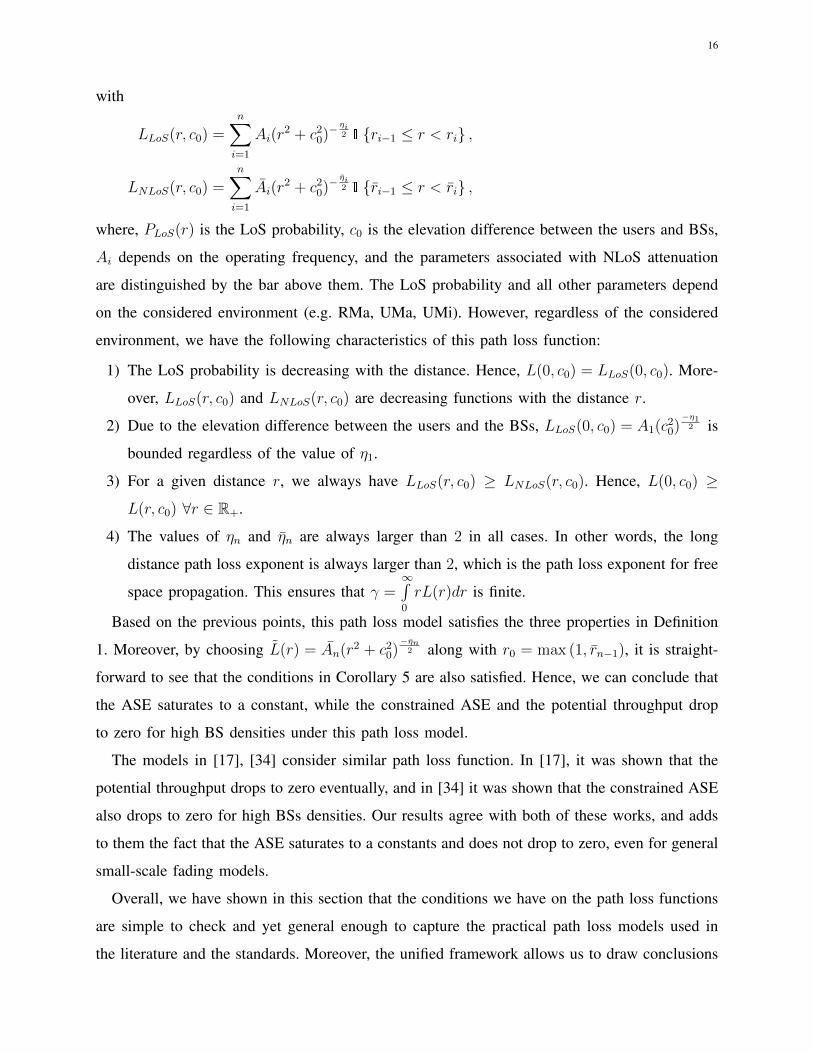
with

LLoS(r, c0) =n∑i=1

Ai(r2 + c2

0)−ηi2 1 {ri−1 ≤ r < ri} ,

LNLoS(r, c0) =n∑i=1

Ai(r2 + c2

0)−ηi2 1 {ri−1 ≤ r < ri} ,

where, PLoS(r) is the LoS probability, c0 is the elevation difference between the users and BSs,

Ai depends on the operating frequency, and the parameters associated with NLoS attenuation

are distinguished by the bar above them. The LoS probability and all other parameters depend

on the considered environment (e.g. RMa, UMa, UMi). However, regardless of the considered

environment, we have the following characteristics of this path loss function:

1) The LoS probability is decreasing with the distance. Hence, L(0, c0) = LLoS(0, c0). More-

over, LLoS(r, c0) and LNLoS(r, c0) are decreasing functions with the distance r.

2) Due to the elevation difference between the users and the BSs, LLoS(0, c0) = A1(c20)−η1

2 is

bounded regardless of the value of η1.

3) For a given distance r, we always have LLoS(r, c0) ≥ LNLoS(r, c0). Hence, L(0, c0) ≥

L(r, c0) ∀r ∈ R+.

4) The values of ηn and ηn are always larger than 2 in all cases. In other words, the long

distance path loss exponent is always larger than 2, which is the path loss exponent for free

space propagation. This ensures that γ =∞∫0

rL(r)dr is finite.

Based on the previous points, this path loss model satisfies the three properties in Definition

1. Moreover, by choosing L(r) = An(r2 + c20)−ηn

2 along with r0 = max (1, rn−1), it is straight-

forward to see that the conditions in Corollary 5 are also satisfied. Hence, we can conclude that

the ASE saturates to a constant, while the constrained ASE and the potential throughput drop

to zero for high BS densities under this path loss model.

The models in [17], [34] consider similar path loss function. In [17], it was shown that the

potential throughput drops to zero eventually, and in [34] it was shown that the constrained ASE

also drops to zero for high BSs densities. Our results agree with both of these works, and adds

to them the fact that the ASE saturates to a constants and does not drop to zero, even for general

small-scale fading models.

Overall, we have shown in this section that the conditions we have on the path loss functions

are simple to check and yet general enough to capture the practical path loss models used in

the literature and the standards. Moreover, the unified framework allows us to draw conclusions

17

regarding the ASE, constrained ASE, and the potential throughput at the same time by checking

the same conditions.

VI. CONCLUSION

We have studied the asymptotic area spectral efficiency (ASE) in a downlink cellular network

under ultradensification. Assuming a Poisson point process for the spatial distribution of the base

stations, a general small-scale fading model, and a class of physically feasible path loss models,

we provided a general framework to analyze the ASE. Our results show that the average ASE

saturates to a constant when the BS density is large, while the constrained ASE and potential

throughput both collapse to zero. These results show that there are fundamental physical limits

to the throughput gains that can be harvested with densification, with the important caveats that

interference is treated as noise and the active user density scales with the base station density.

The results are also all asymptotic with BS density and we do not study when these asymptotics

kick in. These caveats point to interesting future work for dense networks, such as characterizing

at what density the ASE saturation or collapse manifest. Considering the effects of advanced

interference suppression techniques such as joint (over multiple BSs) transmission or decoding,

or successive interference cancellation, would also be of interest.

18

APPENDIX A

PROOF OF LEMMA 1

Let λ = kλ0, where k ∈ Z+ and λ0 ∈ R∗+. We are interested in limk→∞

kλ0SINR(kλ0) which is

found by the following

limk→∞

kλ0SINR(kλ0) = limk→∞

kλ0h0L(r0)∑

ri∈Φ\B(0,r0)

hiL(ri) +N0

= limk→∞

kλ0h0L(r0)∑

ri∈Φ

hiL(ri)− h0L(r0) +N0

= limk→∞

λ0h0L0

1k

∑ri∈Φ

hiL(ri)− h0L0

k+ N0

k

(18)

= limk→∞

λ0h0L0

1k

∑ri∈Φ

hiL(ri)(19)

= limk→∞

λ0h0L0

1k

k∑i=1

∑ri,j∈Ψj

hi,jL(ri,j)

(20)

=λ0h0L0

E

[ ∑ri,1∈Ψ1

hi,1L(ri,1)

] (21)

=λ0h0L0

2πλ0

∞∫0

rL(r)dr

=h0L0

2πγ, (22)

where, (18) follows because L(r0) → L0 a.s. as k → ∞, (19) since as k → ∞, N0

k→ 0 and

h0L0

k→ 0 a.s, (20) by exploiting the superposition property of the PPP [9], where Φ =

∑ki=1 Ψi

and Ψi ∀i ∈ Z∗+ are i.i.d. PPPs each with density λ0, (21) from the law of large numbers,

and (22) from Campbell’s theorem [9]. Note that since the result is independent of λ0, we can

conclude that limλ→∞

λSINR(λ) = h0L0

2πγwhich is finite a.s, hence lim

λ→∞SINR(λ) = 0 a.s, which

completes the proof.

19

APPENDIX B

PROOF OF THEOREM 1

Since we proved the lower bound in Lemma 2, it is sufficient to prove that the asymptotic

ASE is upper bounded by the constant given in (12). The proof is as follows:

limk→∞

E [E(kλ0)] = limk→∞

E [λ0k log2(1 + SINR(kλ0))]

≤ limk→∞

E[λ0

ln(2)kSINR(kλ0)

](23)

= limk→∞

E

λ0

ln(2)k

h0L(r0)∑ri∈Φ\B(0,r0)

hiL(ri) +N0

≤ lim

k→∞E

λ0L0

ln(2)k

h0∑ri∈Φ\B(0,r0)

hiL(ri)

(24)

=λ0L0

ln(2)limk→∞

E

k 1∑ri∈Φ\B(0,r0)

hiL(ri)

, (25)

where, (23) follows since ln(1 + x) ≤ x ∀x ∈ R+, (24) follows because L(r) <= L0 ∀r ∈ R+

and N0 > 0, and (25) by taking the expectation with respect to h0. Next, assuming that the RV

inside the expectation in (25) is uniformly integrable (which we will prove next if I has a finite

second negative moment), then we can push the limit inside the expectation2 [40].

λ0L0

ln(2)limk→∞

E

11k

∑ri∈Φ\B(0,r0)

hiL(ri)

=λ0L0

ln(2)E

limk→∞

11k

∑ri∈Φ\B(0,r0)

hiL(ri)

=

L0

ln(2)2πγ, (26)

where (26) follows from the law of large numbers and Campbell’s theorem similar to the proof

in Lemma 1. Hence, the asymptotic average ASE is upper bounded by L0

ln(2)2πγand we already

proved in Lemma 2 that it is lower bounded by this same constant. Moreover, since the results

hold for all λ0 ≥ λc ∈ R+, then we can conclude that limλ→∞

E [E(λ)] = L0

ln(2)2πγ.

2Precisely, if the RV inside the expectation in (25) is uniformly integrable, then a.s convergence implies convergence in the

L1 norm [40, Theorem 5.5.2].

20

The final step is to prove that the RV inside the expectation in (25) is uniformly integrable if

I has a finite second negative moment, which is proved as follows:

11k

∑ri∈Φ\B(0,r0)

hiL(ri)≤ 1

1k

k∑i=1

∑ri,j∈Ψi\B(0,ri,0)

hi,jL(ri,j)

(27)

=1

1k

k∑i=1

Ii(28)

≤ 1

k

k∑i=1

1

Ii, (29)

where, (27) follows because in the LHS we exclude the closest node to the origin from the

interference and in the RHS we exclude the closest point in each Ψi, where Ψi ∀i are i.i.d.

PPPs with intensity λ0, so we remove the closest BS in Φ and additional ones, (28) by defining

Ii =∑

ri,j∈Ψi\B(0,ri,0)

hi,jL(ri,j), and (29) follows from the convexity of 1/x. Note that in (29),

the random variables 1Ii are i.i.d. and independent from the indexing k. Hence, if 1

Ii has a finite

second moment, then the sequence of RVs (indexed by k) in (29) has a finite second moment

and is uniformly integrable [40, Theorem 5.5.2], which implies that the sequence of RVs in the

LHS of (27) is also uniformly integrable and this concludes the proof.

APPENDIX C

PROOF OF COROLLARY 1

The second negative moment can be written as:

E[

1

I2i

]=

∞∫0

tMI(−t)dt,

whereMI(·) is the moment generating function of the interference I. Using classical stochastic

geometry analysis [15], it can be represented as the following

MI(t) = E[etI]

= E[et∑ri∈Ψ\B(0,r0) L(ri)hi

]=

∫ ∞0

E

∏ri∈Ψ\B(0,r0)

etL(ri)hi |r0

2πλ0e−πλ0r2

0dr0

=

∫ ∞0

exp

(−2πλ0

∫ ∞r

x(1− Eh

[ehtL(x)

])dx

)2πλ0e

−πλ0r20dr0, (30)

21

where (30) follows from the probability generating functional (PGFL) of a PPP [10]. Hence, the

second negative moment of I is given by

E[

1

I2i

]=

∞∫0

∞∫0

2πλ0rt exp

(−πλ0r

2 − 2πλ0

∫ ∞r

x(1− Eh

[e−htL(x)

])dx

)drdt. (31)

From (31), we get the first sufficient condition. The second condition can be found by the

following:

E[

1

I2i

]= E

∑ri∈Ψ\B(0,r0)

L(ri)hi

−2 ≤ E

[(max

ri∈Ψ\B(0,r0)L(ri)hi

)−2]

=

∞∫0

P

((max

ri∈Ψ\B(0,r0)L(ri)hi

)−2

> t

)dt

=

∞∫0

P(

maxri∈Ψ\B(0,r0)

L(ri)hi <1√t

)dt

=

∞∫0

E[1

{max

ri∈Ψ\B(0,r0)L(ri)hi <

1√t

}]dt

=

∞∫0

E

∏ri∈Ψ\B(0,r0)

1

{L(ri)hi <

1√t

} dt =

∞∫0

E

∏ri∈Ψ\B(0,r0)

elog(1

{L(ri)hi<

1√t

}) dt=

∞∫0

∞∫0

2πλ0r exp

−πλ0r2 − 2πλ0

∞∫r

xEh[1− 1

{L(x)h <

1√t

}]dx

drdt (32)

=

∞∫0

∞∫0

2πλ0r exp

−πλ0r2 − 2πλ0

∞∫r

x

[1− Ph

(L(x)h <

1√t

)]dx

drdt, (33)

where (32) follows from the PGFL of a PPP [9].

APPENDIX D

PROOF OF COROLLARY 2

For the Rayleigh fading case, Eh[1− e−htL(x)

]= tL(x)

1+tL(x). By substituting this in the first

condition in the last corollary we get∞∫

0

∞∫0

2πλ0rt exp

(−πλ0r

2 − 2πλ0t

∫ ∞r

xL(x)

1 + tL(x)dx

)drdt = T1 + T2,

22

with

T1 =

∞∫0

r0∫0

2πλ0rt exp

(−πλ0r

2 − 2πλ0t

∫ ∞r

xL(x)

1 + tL(x)dx

)drdt

T2 =

∞∫0

∞∫r0

2πλ0rt exp

(−πλ0r

2 − 2πλ0t

∫ ∞r

xL(x)

1 + tL(x)dx

)drdt. (34)

Then if T1 and T2 are finite, we prove the corollary. Let y0 = L(r0), then

T1 =

∞∫0

r0∫0

2πλ0rt exp

(−πλ0r

2 − 2πλ0t

∫ ∞r

xL(x)

1 + tL(x)dx

)drdt

≤∞∫

0

r0∫0

2πλ0rt exp

(−πλ0r

2 − 2πλ0t

∫ ∞r0

xL(x)

1 + tL(x)dx

)drdt

=

∞∫0

r0∫0

2πλ0rt exp

(−πλ0r

2 − 2πλ0t

∫ y0

0

L−1(y)y

−L′(L−1(y))

1

1 + tydy

)drdt (35)

≤∞∫

0

r0∫0

2πλ0rt exp

(−πλ0r

2 − 2πλ0t

∫ y0

0

ζ

1 + tydy

)drdt (36)

=

∞∫0

r0∫0

2πλ0rt exp(−πλ0r

2 − 2πλ0ζ log(1 + ty0))drdt

=

∞∫0

r0∫0

2πλ0rt exp(−πλ0r

2) 1

(1 + ty0)2πλ0ζdrdt

= (1− e−πλ0r20)

∞∫0

t

(1 + ty0)2πλ0ζdt, (37)

=1− e−πλ0r2

0

y20(2πλ0ζ − 1)(2πλ0ζ − 2)

, (38)

where, (35) follows by the substitution y = L(r), (36) since rL(r)

−L′ (r) ≥ ζ, ∀r ∈ [r0,∞) which

means that L−1(y)y

−L′ (L−1(y))≥ ζ, ∀y ∈ (0, y0 = L(r0)]. Finally, (38) holds as long as λ0 >

1πζ

. Hence

T1 is finite. Moving to T2 defined in (34),

23

T2 =

∞∫0

∞∫r0

2πλ0rt exp

(−πλ0r

2 − 2πλ0t

∫ ∞r

xL(x)

1 + tL(x)dx

)drdt

=

∞∫0

∞∫r0

2πλ0rt exp

(−πλ0r

2 − 2πλ0t

∫ L(r)

0

L−1(y)y

−L′(L−1(y))

1

1 + tydy

)drdt

≤∞∫

0

∞∫r0

2πλ0rt exp

(−πλ0r

2 − 2πλ0t

∫ L(r)

0

ζ

1 + tydy

)drdt (39)

=

∞∫0

∞∫r0

2πλ0rt exp(−πλ0r

2) 1

(1 + tL(r))2πλ0ζdrdt

=

∞∫r0

2πλ0r exp(−πλ0r

2) ∞∫

0

t

(1 + tL(r))2πλ0ζdtdr

=

∞∫r0

2πλ0r exp(−πλ0r

2) 1

bL(r)2dr

=2πλ0

b

∞∫r0

r

L(r)2exp

(−πλ0r

2)dr, (40)

where (39) follows because L−1(y)y

−L′ (L−1(y))≥ ζ, ∀y ∈ (0, y0 = L(r0)] and (40) holds as long as

λ0 ≥ 1πζ

with b = (2πλ0ζ − 2)(2πλ0ζ − 1). The last integral is finite by assumption. Hence, T2

is also finite which proves the corollary.

APPENDIX E

PROOF OF COROLLARY 4

Define I = I/2 =∑

ri∈Ψ\B(0,r0) L(ri)hi, where hi = hi/2, Clearly, if I has a finite second

negative moment, then I will have a finite second negative moment.

E[

1

I2

]=

∞∫0

∞∫0

2πλ0rt exp

(−πλ0r

2 − 2πλ0

∫ ∞r

x(Eh[1− e−htL(x)

])dx

)drdt

≤∞∫

0

∞∫0

2πλ0rt exp

(−πλ0r

2 − 2πλ0t

∫ ∞r

Eh

[x

hL(x)

1 + htL(x)

]dx

)drdt, (41)

24

where (41) follows since 1− e−t ≥ t1+t, ∀t ≥ 0. Moreover,

Eh

[xhL(x)

1 + htL(x)

]=

∞∫0

xhL(x)

1 + htL(x)fH(h)dh

≥1∫

0

xhL(x)

1 + htL(x)fH(h)dh (42)

≥1∫

0

xhL(x)

1 + tL(x)fH(h)dh =

xL(x)

1 + tL(x)P{h ≤ 1

}≥ 1

2

xL(x)

1 + tL(x), (43)

where fH(·) is the probability density function (PDF) of h. (42) follows since the integrand is

positive and (43) since by Markov’s inequality P{h ≤ 1

}≥ 1− E[h] = 1

2. Hence,

E[

1

I2

]≤

∞∫0

∞∫0

2πλ0rt exp

(−πλ0r

2 − πλ0t

∫ ∞r

xL(x)

1 + tL(x)dx

)drdt.

Then the proof follows as in the proof of Corollary 2.

REFERENCES

[1] M. S. Alouini and A. J. Goldsmith, “Area spectral efficiency of cellular mobile radio systems,” IEEE Trans. on Veh.

Technology, vol. 48, no. 4, pp. 1047–1066, Jul. 1999.

[2] V. Chandrasekhar, J. G. Andrews, and A. Gatherer, “Femtocell networks: a survey,” IEEE Communications Magazine,

vol. 46, no. 9, pp. 59–67, Sep. 2008.

[3] ArrayComm, “http://www.arraycomm.com/technology/coopers-law/.”

[4] Qualcomm, “The 1000x data challenge,” https://www.qualcomm.com/invention/technologies/1000x/small-cells.

[5] J. G. Andrews, S. Buzzi, W. Choi, S. Hanly, A. Lozano, A. Soong, and C. Zhang, “What will 5G be?” IEEE Journal on

Selected Areas in Communications, June 2014.

[6] P. Gupta and P. R. Kumar, “The capacity of wireless networks,” IEEE Trans. on Info. Theory, pp. 388–404, Mar. 2000.

[7] F. Xue and P. R. Kumar, “Scaling laws for ad hoc wireless networks: an information theoretic approach,” Foundations and

Trends in Networking, vol. 1, no. 2, pp. 145–270, 2006.

[8] M. Franceschetti, M. Migliore, and P. Minero, “The capacity of wireless networks: Information-theoretic and physical

limits,” IEEE Trans. on Info. Theory, vol. 55, no. 8, pp. 3413–24, Aug. 2009.

[9] F. Baccelli and B. Błaszczyszyn, “Stochastic geometry and wireless networks: Volume I theory,” Foundations and Trends R©

in Networking, vol. 3, no. 3–4, pp. 249–449, 2010.

[10] ——, “Stochastic geometry and wireless networks: Volume II applications,” Foundations and Trends R© in Networking,

vol. 4, no. 1–2, pp. 1–312, 2010.

[11] M. Haenggi, Stochastic Geometry for Wireless Networks. Cambridge University Publishers, 2012.

25

[12] H. ElSawy, A. Sultan-Salem, M. S. Alouini, and M. Z. Win, “Modeling and analysis of cellular networks using stochastic

geometry: A tutorial,” IEEE Communications Surveys & Tutorials, vol. 19, no. 1, pp. 167–203, Firstquarter 2017.

[13] F. Baccelli, B. Blaszczyszyn, and P. Muhlethaler, “An ALOHA protocol for multihop mobile wireless networks,” IEEE

Transactions on Information Theory, vol. 52, no. 2, pp. 421–436, February 2006.

[14] S. Weber, X. Yang, J. G. Andrews, and G. de Veciana, “Transmission capacity of wireless ad hoc networks with outage

constraints,” IEEE Trans. on Info. Theory, vol. 51, no. 12, pp. 4091–4102, Dec. 2005.

[15] J. G. Andrews, F. Baccelli, and R. K. Ganti, “A tractable approach to coverage and rate in cellular networks,” IEEE Trans.

on Communications, vol. 59, no. 11, pp. 3122–3134, Nov. 2011.

[16] H. S. Dhillon, R. K. Ganti, F. Baccelli, and J. G. Andrews, “Modeling and analysis of K-tier downlink heterogeneous

cellular networks,” IEEE Journal on Sel. Areas in Communications, vol. 30, no. 3, pp. 550–560, April 2012.

[17] I. Atzeni, J. Arnau, and M. Kountouris, “Downlink cellular network analysis with LoS/NLoS propagation and elevated

base stations,” IEEE Trans. on Wireless Communications, Oct. 2017, to appear.

[18] A. AlAmmouri, J. G. Andrews, and F. Baccelli, “SINR and throughput of dense cellular networks with stretched exponential

path loss,” IEEE Trans. on Wireless Communications, Nov. 2017, to appear.

[19] X. Zhang and J. G. Andrews, “Downlink cellular network analysis with multi-slope path loss models,” IEEE Trans. on

Communications, vol. 63, no. 5, pp. 1881–1894, May 2015.

[20] M. Ding, P. Wang, D. Lopez-Perez, G. Mao, and Z. Lin, “Performance impact of LoS and NLoS transmissions in dense

cellular networks,” IEEE Trans. on Wireless Communications, vol. 15, no. 3, pp. 2365–2380, Mar. 2016.

[21] M. D. Renzo, W. Lu, and P. Guan, “The intensity matching approach: A tractable stochastic geometry approximation to

system-level analysis of cellular networks,” IEEE Trans. on Wireless Communications, vol. 15, no. 9, pp. 5963–5983, Sep.

2016.

[22] N. Lee, F. Baccelli, and R. W. Heath, “Spectral efficiency scaling laws in dense random wireless networks with multiple

receive antennas,” IEEE Trans. on Info. Theory, vol. 62, no. 3, pp. 1344–1359, Mar. 2016.

[23] T. Bai, R. Vaze, and R. W. Heath, “Analysis of blockage effects on urban cellular networks,” IEEE Trans. on Wireless

Communications, pp. 5070–83, Sept. 2014.

[24] S. Rangan, T. Rappaport, and E. Erkip, “Millimeter-wave cellular wireless networks: Potentials and challenges,” Proceedings

of the IEEE, vol. 102, no. 3, pp. 366–385, Mar. 2014.

[25] 3GPP TR 36.814, in Further Advancements for E-UTRA Physical Layer Aspects (Release 9),

http://www.3gpp.org/ftp/Specs/archive/36series/36.814/36814-900.zip, Mar. 2010.

[26] 3GPP TR 38.901, in Study on channel model for frequencies from 0.5 to 100 GHz (Release 14),

http://www.3gpp.org/ftp/Specs/archive/38series/38.901/38901-e20.zip, Sep. 2017.

[27] K. Huang and J. G. Andrews, “An analytical framework for multicell cooperation via stochastic geometry and large

deviations,” IEEE Trans. on Info. Theory, vol. 59, no. 4, pp. 2501–2516, Apr. 2013.

[28] S. P. Weber, J. G. Andrews, X. Yang, and G. de Veciana, “Transmission capacity of wireless ad hoc networks with

successive interference cancellation,” IEEE Trans. on Info. Theory, vol. 53, no. 8, pp. 2799–2814, Aug. 2007.

[29] F. Baccelli, A. El Gamal, and D. Tse, “Interference networks with point-to-point codes,” IEEE Trans. on Info. Theory,

vol. 57, no. 5, pp. 2582–2596, May 2011.

[30] X. Zhang and M. Haenggi, “The performance of successive interference cancellation in random wireless networks,” IEEE

Trans. on Info. Theory, vol. 60, no. 10, pp. 6368–6388, Oct. 2014.

[31] S. Shamai and A. D. Wyner, “Information-theoretic considerations for symmetric, cellular, multiple-access fading channels.

I,” IEEE Trans. on Info. Theory, vol. 43, no. 6, pp. 1877–1894, Nov. 1997.

26

[32] G. Chen, L. Qiu, and Z. Chen, “Area spectral efficiency analysis of multi-antenna networks modeled by Ginibre point

process,” IEEE Wireless Communications Letters, 2017, to appear.

[33] A. M. Alam, P. Mary, J. Y. Baudais, and X. Lagrange, “Asymptotic analysis of area spectral efficiency and energy efficiency

in PPP networks with SLNR precoder,” IEEE Trans. on Communications, vol. 65, no. 7, pp. 3172–3185, Jul. 2017.

[34] M. Ding and D. Lopez-Perez, “Performance impact of base station antenna heights in dense cellular networks,” IEEE

Trans. on Wireless Communications, vol. 16, no. 12, pp. 8147–8161, Dec. 2017.

[35] C. Li, J. Zhang, J. G. Andrews, and K. B. Letaief, “Success probability and area spectral efficiency in multiuser MIMO

hetnets,” IEEE Trans. on Communications, vol. 64, no. 4, pp. 1544–1556, Apr. 2016.

[36] M. Afshang, H. S. Dhillon, and P. H. J. Chong, “Modeling and performance analysis of clustered device-to-device networks,”

IEEE Trans. on Wireless Communications, vol. 15, no. 7, pp. 4957–4972, Jul. 2016.

[37] H. Royden, Real Analysis, ser. Mathematics and statistics. Macmillan, 1988.

[38] J. G. Andrews, X. Zhang, G. D. Durgin, and A. K. Gupta, “Are we approaching the fundamental limits of wireless network

densification?” IEEE Communications Magazine, vol. 54, no. 10, pp. 184–190, Oct. 2016.

[39] J. G. Andrews, T. Bai, M. N. Kulkarni, A. Alkhateeb, A. K. Gupta, and R. W. Heath, “Modeling and analyzing millimeter

wave cellular systems,” IEEE Trans. on Communications, vol. 65, no. 1, pp. 403–430, Jan. 2017.

[40] R. Durrett, Probability: theory and examples. Cambridge university press, 2010.

[41] S. M. Yu and S. L. Kim, “Downlink capacity and base station density in cellular networks,” in Proc. International

Symposium on Modeling and Optimization in Mobile, Ad Hoc, and Wireless Networks (WiOpt), May 2013, pp. 119–124.

[42] M. Hata, “Empirical formula for propagation loss in land mobile radio services,” IEEE Trans. on Veh. Technology, vol. 29,

no. 3, pp. 317–325, Aug. 1980.

[43] I. Trigui, S. Affes, and B. Liang, “Unified stochastic geometry modeling and analysis of cellular networks in LOS/NLOS

and shadowed fading,” IEEE Trans. on Communications, 2017, to appear.

[44] A. AlAmmouri, H. ElSawy, A. Sultan-Salem, M. D. Renzo, and M. S. Alouini, “Modeling cellular networks in fading

environments with dominant specular components,” in Proc., IEEE Intl. Conf. on Communications, May 2016, pp. 1–7.

[45] J. Liu, M. Sheng, L. Liu, and J. Li, “Effect of densification on cellular network performance with bounded pathloss model,”

IEEE Communications Letters, vol. 21, no. 2, pp. 346–349, Feb. 2017.

[46] A. Goldsmith, Wireless communications. Cambridge university press, 2005.

[47] T. Rappaport, Wireless Communications: Principles and Practice, 2nd ed. Prentice Hall PTR, 2001.