Clemson UniversityTigerPrints

All Theses Theses

8-2018

A Visual Data Analysis of the Toxics ReleaseInventoryTheodore Charles LangloisClemson University, tlanglo@clemson.edu

Follow this and additional works at: https://tigerprints.clemson.edu/all_theses

This Thesis is brought to you for free and open access by the Theses at TigerPrints. It has been accepted for inclusion in All Theses by an authorizedadministrator of TigerPrints. For more information, please contact kokeefe@clemson.edu.

Recommended CitationLanglois, Theodore Charles, "A Visual Data Analysis of the Toxics Release Inventory" (2018). All Theses. 2929.https://tigerprints.clemson.edu/all_theses/2929

A VISUAL DATA ANALYSIS OF THE TOXICS RELEASE INVENTORY

A Thesis

Presented to

the Graduate School of

Clemson University

In Partial Fulfillment

of the Requirements for the Degree

Master of Science

Environmental Engineering and Earth Sciences

by

Theodore Charles Langlois

August 2018

Accepted by:

Dr. Elizabeth Carraway, Committee Co-Chair Dr.

Michael Carbajales-Dale, Committee Co-Chair

Dr. David Ladner

ii

ABSTRACT

The Environmental Protection Agency’s Toxics Release Inventory (TRI) is a

collection of data detailing the way hazardous chemicals are handled in industrial

facilities. By requiring certain manufacturing facilities to report releases, the EPA

offered the public unprecedented access to environmentally relevant data. Since its

inception in 1986, the TRI has grown and changed both in chemicals and industries

monitored. This thesis uses the data visualization platform Tableau, publicly available

yearly TRI reports, and Life cycle impact assessment methodology to create a tool which

1) improves upon previous analyses of the TRI dataset, 2) offers an analysis based on

previously underexplored environmental impacts, and 3) creates a simple online tool for

communities, industry, and government to use to better identify and target problem areas.

iii

ACKNOWLEDGEMENTS

Thank you to my committee, Dr. Carraway, Dr. Dale, and Dr. Ladner for supporting me

through the E3 grant, as well as providing insights into my project, gathering data, and

directing the research into the quagmire that is Toxics Release Inventory data.

Also, a big thank you to John Sherwood for introducing me to Tableau and his

willingness to allow me to bounce ideas off him from across the office.

Thank you, Margaret Thompson, for being a friend and mentor and supporting my

interest in Environmental Policy.

Thank you, E3SA research group members, current and former, for your academic

interest and sharp minds.

Lastly, thank you to my friends and family who are always a call away and always

supportive.

iv

TABLE OF CONTENTS

Page

TITLE PAGE .................................................................................................................... i

ABSTRACT ..................................................................................................................... ii

ACKNOWLEDGMENTS .............................................................................................. iii

LIST OF FIGURES ........................................................................................................ vi

LIST OF TABLES ......................................................................................................... vii

CHAPTER

I. INTRODUCTION ......................................................................................... 1

South Carolina E3: Energy-Economy-Environment ............................... 1

Motivation and Goal ................................................................................ 1

II. BACKGROUND ........................................................................................... 3

Existing Data: The Toxics Release Inventory ......................................... 3

TRI Successes .......................................................................................... 6

TRI Challenges and Failures .................................................................... 8

Existing Models and Tools .................................................................... 10

Conceptualizing an Ideal Tool ............................................................... 16

Developing the Ideal Tool ..................................................................... 18

Introduction to Life Cycle Assessment .................................................. 18

TRI as a Subset of the US Economy ...................................................... 24

Previous Work and Other Analyses ....................................................... 25

III. METHODS .................................................................................................. 28

Tableau ................................................................................................... 28

TRI Data................................................................................................. 29

TRACI.................................................................................................... 30

NAICS Codes and Descriptions............................................................. 30

Data Integration ..................................................................................... 31

Tableau Workbook Publication ............................................................. 32

Improvements on Existing Tools ........................................................... 32

v

Table of Contents (Continued)

Page

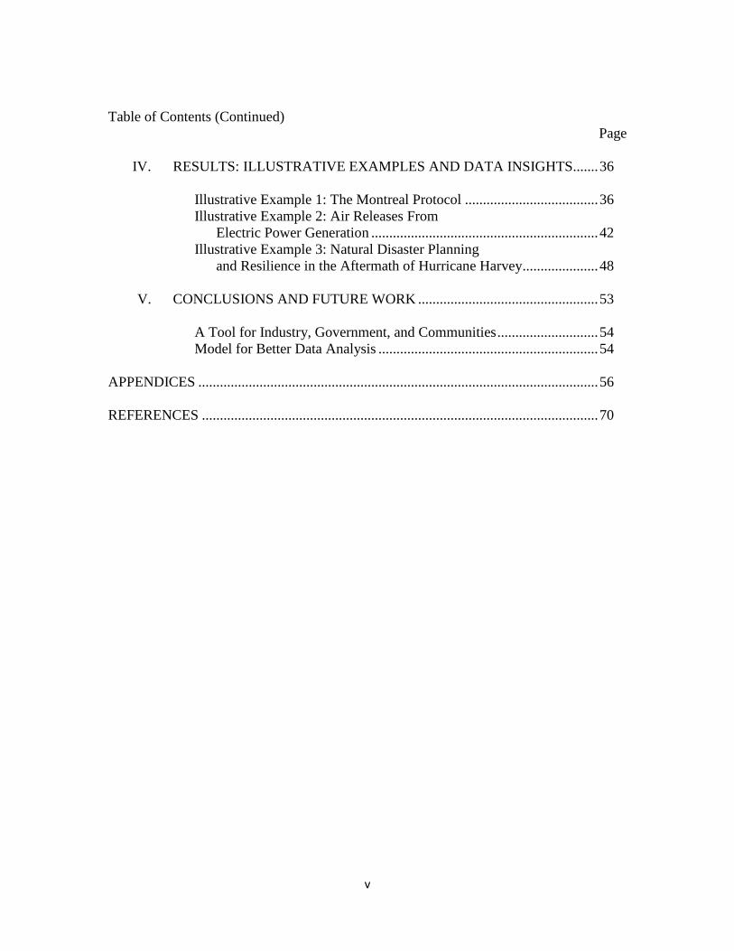
IV. RESULTS: ILLUSTRATIVE EXAMPLES AND DATA INSIGHTS....... 36

Illustrative Example 1: The Montreal Protocol ..................................... 36

Illustrative Example 2: Air Releases From

Electric Power Generation ............................................................... 42

Illustrative Example 3: Natural Disaster Planning

and Resilience in the Aftermath of Hurricane Harvey ..................... 48

V. CONCLUSIONS AND FUTURE WORK .................................................. 53

A Tool for Industry, Government, and Communities ............................ 54

Model for Better Data Analysis ............................................................. 54

APPENDICES ............................................................................................................... 56

REFERENCES .............................................................................................................. 70

vi

LIST OF FIGURES

Figure Page

1.1 A Visual Timeline of the TRI Program ......................................................... 5

2.1 Hierarchy of Environmentally Preferable Methods

of Waste Management ........................................................................... 10

2.2 Breakdown by Method of Hazardous Waste

Managed in the US in 2016 ................................................................... 10

2.3 Phases of an LCA......................................................................................... 19

2.4 Stages of a Life Cycle .................................................................................. 19

2.5 Flow of Information in a Life Cycle Impact Assessment ............................ 21

2.6 Impact Categories and Pathways Covered by

The IMPACT 2002+ Methodology ....................................................... 23

3.1 Entity Relationship Diagram for TRI Data Management ............................ 31

3.2 EPA National Analysis Fact Sheet, South Carolina 2016 ........................... 33

3.1 Tableau-produced Ecotoxicity Analysis, South Carolina 2016 ................... 33

4.1 Ozone Depleting TRI Chemicals 1986-2016 ............................................... 39

4.2 TRI Greenhouse Gasses 1986-2016 ............................................................. 41

4.3 Total TRI Air Releases 1986-2016 .............................................................. 43

4.4 Non-HCl Air Releases 1986-2016 ............................................................... 44

4.5 Recorded HCl Emissions 1986-2016 ........................................................... 46

4.6 Map of Observed Flood Extent with TRI Facilities..................................... 50

4.7 Chemical Inventory for Potentially Flooded

Texas TRI Facilities – Top 10 by Mass ................................................. 52

vii

4.8 Chemical Inventory for Potentially Flooded

Texas TRI Facilities – Top 10 by Ecotoxicity ....................................... 52

List of Figures (Continued) Page

viii

LIST OF TABLES

Table Page

2.1 Description of Results from RSEI Model .................................................... 15

2.2 Existing Reports Utilizing TRI Data............................................................ 16

4.1 Global Warming Potentials of Selected

Greenhouse Gases .................................................................................. 38

1

1 INTRODUCTION

1.1 SOUTH CAROLINA E3: ENERGY-ECONOMY-ENVIRONMENT

The South Carolina Economy, Energy, Environment (SCE3) program began as a

Pollution Prevention (P2) grant from the Environmental Protection Agency (EPA). It is a

collaboration between partners Clemson University, Duke Energy, South Carolina

Manufacturing Extension Partnership (SCMEP), and South Carolina Department of

Health and Environmental Control (DHEC). SCE3 uses community resources to provide

technical assistance to small- to medium-sized manufacturers in upstate South Carolina in

the form of energy, waste, and lean business audits. The program helps drive sustainable

manufacturing by reducing energy and material waste while increasing efficiency and

productivity. Pursuant to SCE3’s waste reduction mission, this research explores trends

in industrial waste management, including pollution prevention practices and changes in

national hazardous waste policy.

1.2 MOTIVATION AND GOAL

SC E3 provides facility-level technical assistance to manufacturers, which requires

direct contact with individual companies. This hands-on approach is useful when

assisting manufacturers who reach out for auditing and benchmarking. However, without

site visits from trained auditors or an in-depth understanding of yearly releases,

companies may not fully understand how their facility compares to others in the industry,

geographic area, or type of chemical processing. The goal of this project is to fill such

2

knowledge gaps and provide a national-level, impact-based view of chemical release

trends, through the creation of an interactive online tool. This tool will provide

legislators, facilities, industry groups, and various levels of government the opportunity

to track releases geographically and over time to identify trends in hazardous chemical

use and release without inside knowledge of any specific facility or industry.

3

2 BACKGROUND

2.1 EXISTING DATA – TOXICS RELEASE INVENTORY

In December of 1984, approximately 40 metric tons of methyl isocyanate

(CH3NCO) gas was accidentally released at a Union Carbide plant in Bhopal, India. The

resulting cloud of gas killed between 2,000 and 4,000 people in the city and many more

were hospitalized (Broughton, 2005). The Bhopal incident is still considered to be the

worst industrial accident in history. Public concern after this event and several smaller

accidents in the United States was enough to spur lawmakers into action. In 1986,

Congress passed the Emergency Planning and Community Right-to-Know Act (EPCRA)

(Koehler, 2007). This act sought to prepare industries and communities for such disasters

and reduce the likelihood of their occurrence through planning and regulation of

hazardous chemicals. If community members are informed about industrial actives, they

can exert influence over facilities that may be releasing toxic chemicals to their local

environments. Thus, a new planning, reporting, and emergency notification system

emerged (EPA 1986).

Under Section 313 of EPCRA the EPA created a list of hazardous chemicals to be

tracked by the sitting administrator. Facilities which handle the listed chemicals above

threshold amounts, unique to each chemical, are required to report use of those chemicals

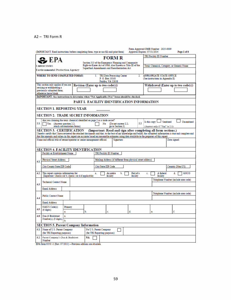
to the EPA via a special reporting document called “Form R,” which can be found in

Appendix A. This form identifies the company, its location, industry classification, the

4

chemical and its method of management. These management categories are informed by

EPA’s Pollution Prevention Hierarchy and include direct releases to air, water, or land, as

well as waste management categories such as “on-site recycling processes,” and “off-site

treatment” (EPA 2017). By collecting reports of these metrics, EPA built what is known

as the Toxics Release Inventory (TRI). The data exist as series of spreadsheets, yearly

reports, and an online tool that provides the public with general information on facilities

and industries that handle hazardous chemicals. Figure 1 is a visual timeline of the TRI

program and details changes and updates to reporting.

5

Figure 1.1 A Visual Timeline of the TRI Program

6

2.2 TRI SUCCESSES

The TRI program offers an unprecedented amount of data to the public. In a way

that no public policy had done previously, it put power in the hands of citizens by

creating a transparent system of pollution reporting.

2.2.1 A Novel Approach

Often cited as some of the most successful environmental legislation, TRI is at its

simplest level, a collection of data detailing legal releases, transfers, treatment, and

recycling of hazardous chemicals. Manufacturing facilities acquire permits for each

chemical handled and report their use as required by law. EPA rarely inspects reporting

facilities and emissions are often estimated rather than stringently measured. This variety

of informal regulation was relatively novel, and unexpectedly successful. Instead of

fining and penalizing companies for non-compliance, TRI relies on transparency.

Reported releases become public record and can serve as leverage for community

activists or government agencies wishing to apply pressure on manufacturers to change

their behavior. Its success hinges on free and open access to data and the ability of

outsiders to identify trends and use them to influence corporations, not to mention the

honesty in company reporting. In a 2000 EPA press release, then Vice President Al Gore

said:

Putting basic information about toxic releases into the hands of citizens is one of the most powerful tools available for protecting public health and the environment in local communities. That is why this Administration has

7

dramatically expanded the public’s access to this vital information. Citizens now have more information than ever at their fingertips to help protect their communities, their health and their children’s health. (EPA Press Release, 2000)

Simply measuring the release of toxic chemicals seems to be the first step in achieving

reductions. In 1995, the 9th year of the program, the EPA reported a decrease in total

releases and transfers of 45% since 1988 (Fung and O’Rourke, 2000). While the

reduction reported cannot be completely attributed to TRI data collection, its availability

certainly influenced industry action on improving pollution control technologies and

process efficiency.

2.2.2 Measured Success

Other studies, such as that performed by Koh et al. (2016) seem to confirm that the

reduction trend which began in the early years of TRI continued between 1999 and 2009.

Using an input-output structural decomposition analysis (SDA), the authors were able to

combine the TRI dataset with information about population growth, consumption of

goods and services per capita in the US, and changes in input mix (use of domestic or

imported materials). The resulting analysis identifies drivers of the Toxicological

Footprint (TF) within the US economy. The authors measured a 39% decrease in TF

between 1999 and 2013 due to improvements in production efficiency, despite increases

in both consumption volume (8%) and population (10%), which would ordinarily

increase the TF. It is reasonable to attribute this decrease to a collective transition to

cleaner methods of production across various manufacturing industries. Interestingly, the

authors also measured a 14.1% increase in TF between 2009 and 2013, due to a

combination of factors including economic growth during recovery from a recession, an

8

increase in consumption volume, and population growth, which combined to nullify a

measured 4% improvement in emissions intensity. In general, the TRI and associated

EPA programs encouraging reduction activities have driven increases in production

efficiency and subsequent decreases in emissions intensity – in this case, the ratio of

chemical emitted per unit of product produced.

Additional benefits of the TRI include its ability to flag particularly toxic

chemicals, including those known to cause cancer. Between 1995 and 1999, emission of

chemicals designated as “carcinogens” decreased 16%, while total releases decreased

only 7% (Graham and Miller 2001). Not only does the TRI system encourage reduction

of toxic chemicals through data transparency, it is structured to identify and reduce the

most toxic of these first, based on simple data.

2.3 TRI CHALLENGES AND FAILURES

2.3.1 Data Accuracy

Despite its apparent success, the TRI is not a one-size-fits-all solution to production

waste. As a result of its light regulation on industry, the inventory itself contains

mistakes, estimates, and an occasional data gap. In the program’s first year, the EPA

estimated that 10,000 of about 30,000 facilities required to report failed to do so (Wolf

1996). A 1990 General Accounting Office (GOA) study of the program found non-

reporting to be a significant issue that stemmed from “inefficient strategies to identify

non-reporters,” and the “absence of explicit authority under [EPCRA] to inspect facilities

for compliance” (GOA 1990). Additionally, choice of reporting category, often left up to

9

the discretion of the facility manager, can affect results. “Paper changes,” in which the

disposal category is changed from one year to the next, were found to account for more

than half of reductions between 1991 and 1994 in one study (Natan and Miller, 1998).

By “redefining on-site recycling activities as in-process recovery,” facilities avoided the

necessity of reporting to a TRI waste management category. The result does not reflect a

physical change in the manufacturing process, but to an outside party, and without

additional information, it could appear to be a reduction.

This, however, is not to say that the TRI is not a useful data set for environmental

scientists, industry professionals, lawmakers, and community members. Despite its

flaws, the inventory still represents the most comprehensive gathering of hazardous

chemical data available. Graham and Miller (2001) call it “an evolutionary bridge

between familiar national policies that treated information as a public right and emerging

strategies that employ information as regulation.” Despite data issues in the early years

of the program, the EPA provides a series of checks on data accuracy and completeness.

EPA’s data quality group provides guidance during the reporting period through an

online tool and a reporting “hotline” (TRI Data Quality 2018). Unusual release

characteristics such as large increases or decreases from the previous year or increases of

releases of persistent bioaccumulative toxics (PBTs) are flagged and the facilities in

questions are contacted.

10

2.4 EXISTING MODELS AND TOOLS

2.4.1 TRI National Analysis

In the age of big data, we have access to even more information than VP Gore

spoke about 18 years ago. TRI data are available to anyone with internet access, as is

EPA’s TRI National Analysis. The TRI National Analysis “summarizes recently

submitted TRI data, trends, special topics, and interprets the findings from the

perspective of EPA’s mission to protect human health and the environment” (EPA,

2016). The Pollution Prevention Act of 1990 the chemicals managed are broken down

into categories and arranged hierarchically by environmental preferability, as shown in

Figure 2.1. It begins with source reduction, which deals with preventing hazardous by-

products from being produced, followed by methods for managing hazardous material

after it is created.

Figure 2.1 Hierarchy of Environmentally Prefereable

Methods of Waste Management (EPA)

Figure 2.2 Breakdown by Method of Hazardous Waste

Managed in the US in 2016 (TRI National Analysis 2016)

11

Source reduction is “any practice that reduces, eliminates, or prevents pollution at its

source” (EPA 2018). The name implies that the waste is never produced, for example by

adjusting a process so that non-toxic chemicals are used in place of toxic ones. EPA

considers source reduction the most preferable option.

Recycling, the next most preferable method of waste management, is any process that

allows a chemical to be “used or reused, [or] reclaimed”. Reclaimed materials are

recovered as a useable product or regenerated to again become an input for a process.

Used or reused materials are either used as an ingredient to make a product or are used as

an “effective substitute for a commercial product.” (EPA 2017)

Energy Recovery is technically a subset of recycling, but instead of a material becoming

a feedstock for additional processes, the substance is combusted for heat or combined

heat and power. For example, the data shows that hundreds of millions of kilograms of

ethene are combusted on-site annually at chemical manufacturing plants in the US.

Using waste ethene as a heating fuel helps a facility reduce costs and environmental

impacts of bringing in additional heating sources.

Treatment constitutes a process that “modifies the chemical properties of the waste, for

example, through reduction of water solubility or neutralization of acidity or alkalinity”

(Glossary of Environment Statistics 1997).

Release, as its name implies, refers to any hazardous chemical that is emitted without

additional treatment or processing. It can be a purposeful release from a stack, a fugitive

12

releases from leaks, direct discharges to surface water, or land releases which include

underground injection, surface impoundments, or landfills.

These categories make up the basis for claims of improvement; reduction in less

favorable categories and shifts to a more preferable category are seen as strides forward,

as they certainly should be.

However, not all chemical releases are created equally. TRI data are reported in

terms of pounds of chemical, and the National Analysis is produced using these same

metrics. For example, the pesticide Cyfluthrin has a LD50 of 380 mg/kg for rats is

compared to a less toxic compound like methanol, with a LD50 of 5628 mg/kg (Cyfluthrin

and Methanol MSDS). Thus, for the rat fatality endpoint, a pound of Cyfluthrin is nearly

fifteen times more potent than a pound of methanol. Cyfluthrin is also highly toxic in the

aquatic environment. Further analysis will show that while methanol has the potential to

cause damage to ecosystems, it is five orders of magnitude less toxic in freshwater than

Cyfluthrin (TRACI 2002). In terms of production scale, it may be easier to reduce

releases of methanol and its history of reduction may be found in the TRI data.

Additionally, because toxicity data are not included in the analysis, reductions may

appear to be more significant without adjustment for the chemical’s toxicity. A better

understanding of the relationship between mass and toxicity is important for facilities to

understand when choosing chemicals to target for reduction.

Figure 2.2 shows the fate of TRI chemicals for the calendar year 2016. When

viewed strictly in terms of mass, 27.80 billion pounds of waste appears to be a large

13

amount, but absent toxicological data, the importance of the management cannot be

effectively quantified. This is not to say that the National Analysis is not an important

tool. It is effective in communicating trends in waste management, information

comparing industry sectors, and increases or decreases of specific chemical use. It

presents an accessible tool to businesses, local, state, and federal government, interest

groups, and citizens so that they may better understand the chemicals used in their

industries, constituencies, and communities. The availability of this data assists with

emergency planning, lobbying, exerting public pressure on facilities, and identifying

needs and opportunities for source reduction (Fung and O’Rourke 2000). However, it

does little to directly inform risk-based decisions.

2.4.2 Risk-Screening Environmental Indicators model.

Similar to the TRI National Analysis, EPA’s Risk-Screening Environmental

Indicators (RSEI) model intends to make hazardous chemical release data accessible to

the public. Unlike the National Analysis, or interpretation of raw TRI data, the RSEI

method uses toxicity and chemical transport models to give “a screening-level, risk-

related perspective for relative comparisons of chemical releases” (EPA 2018). Using the

model, it is possible to compare chemicals based on toxicity rather than mass alone.

Although the model does not estimate actual risk to individuals, it performs an important

14

function: it links empirical data with science-based, environmental fate and transport

models for public consumption.

The EPA hosts a user-friendly, web-based model which allows the user to sort

through TRI data using various metrics, including region, chemical, industry, and

individual facility. For each of these categories, EPA defines risk as measured by “RSEI

Score,” a “unitless measure that is not independently meaningful, but is a risk-based

estimate that can be compared to other estimates calculated using the same method (RSEI

Methodology, p. ES-7).” RSEI leverages EPA methodologies for measuring toxicity,

including the Integrated Risk Information System (IRIS), and chooses toxicity data based

on a hierarchical system, opting for EPA and consensus data sources over others. In

addition to toxicity data, RSEI successfully introduces geospatial, meteorological, and

environmental fate and transport elements using an air dispersion model AERMOD (EPA

Support Center for Regulatory Atmospheric Modeling) and the National Hydrography

Dataset (US Geological Survey). This coupled approach allows for the public to increase

their awareness of the types of chemicals released by TRI facilities, as well as the role

that climate and geography play in their transport.

15

Table 2.1 Description of Results from RSEI Model, EPA’s RSEI Methodology, p. ES-7

Table 2.1 shows the three types of results gained from RSEI. Clearly, at each

stage complexity of information increases, and the model becomes more useful for

certain purposes. Pounds-based results are similar to information from the National

Analysis with the key improvement being that RSEI data are coupled with an

environmental fate and transport model. Hazard-based results expand upon the mass-

based data by adding toxicity weighting. This is the key to establishing data that are

comparable between different chemicals. Finally, the risk-related results multiply the

surrogate dose – the concentration that is to be expected in ambient air or drinking water

– by the toxicity weight and finally a population factor. While it is not specifically

dedicated to evaluating trends in toxic releases, nor does it quantify risk, nor provide

metrics on ecosystem damage, RSEI provides an easy-to-use platform backed by real-life

toxicity data, making it a valuable tool for addressing pollution.

Description of RSEI Results

Risk-related results (scores) Surrogate Dose x Toxicity Weight x

Population

Hazard-based results Pounds x Toxicity Weight

Pounds-based results TRI Pounds Released

16

2.5 CONCEPTUALIZING AN IDEAL TOOL

An ideal tool fills methodological gaps in the National Analysis and RSEI

methods as shown below in Table 2.2. Such a tool addresses the lack of toxicity

considerations in the National Analysis, while providing a quantifiable impact-based

assessment of environmental and human health effects to contrast with the risk-based

RSEI model. Risk-based models like RSEI account for chemical toxicity, expected

exposure dose, and population. RSEI specifically calculates a “risk score” which can be

used to compare exposure to one or more chemicals. Essentially, it ranks the likelihood

of a person in a location with set ambient air characteristics to experience various

negative health consequences due to chemical exposure. Because this type of model is

anthropocentric, it focuses only on chemicals which impact human health, whether

through chronic or carcinogenic effects. Impact-based models seek to link chemical

Table 2.2 - Existing Reports Utilizing TRI Data

Yearly Analyses of the Toxics Release Inventory

Report TRI National Analysis Risk-Screening Environmental

Indicators

Description

Mass-based release trends Risk-based model using EPA IRIS

Deficiencies No connection of chemicals to impacts

Lacks ecological considerations

Limited scope and timeline Calculates aggregated Risk “Scores” for comparison only

17

releases to a specific endpoint, or impact. While RSEI calculates a risk score to

provide a basis of comparison, the score represents an aggregate risk to human health and

does not provide information on type of health hazard which could be expected as a result

of exposure to a certain chemical. An impact-based tool addresses multiple types of

impacts. Given a specific discharge of a chemical to a chosen media, an impact-based

model could predict, to some degree of accuracy, its effect on plants and animals in the

environment or environmental quality.

The ideal tool would leverage the advantages of the breadth of data provided by

TRI, the transport and exposure pathways utilized in the RSEI model and incorporate an

impact-focused component to quantitatively evaluate the consequences of releases in

terms of measurable environmental effects such as toxicity to organisms or health hazards

for humans. The tool also emphasizes utility; it provides instant visualizations based on

geographic location, chemical, industry, and specific impact. Meeting these goals

requires a number of important components. The ideal tool combines the TRI data,

specifying facility-level data, detailed explanations of industry codes, a protocol for

evaluating chemical impact on the environment, and a visualization program able to read

and sort large amounts of chemical and industrial data. The convergence of these

constituent parts would allow a person unfamiliar with the TRI system and no knowledge

of manufacturing to sift through historical and scientific data to find and identify

important chemical trends.

18

2.6 DEVELOPING THE IDEAL TOOL

The first step to developing an impact-based tool requires selection of impact

categories and a method for relating chemical releases to these impacts, which will be

discussed later. We assume that the TRI data set can be considered an inventory of

physical flows, in this case, elementary chemical flows into the environment. Under this

assumption, it is possible to use the framework of life cycle assessment (LCA),

specifically life cycle impact assessment (LCIA), to evaluate the environmental

consequences of the release of hazardous chemicals to the environment. To understand

the principles of impact assessment and how they can play a role in creating a useful tool,

it is important to understand the basics of LCA.

2.7 INTRODUCTION TO LIFE CYCLE ASSESSMENT

2.7.1 Basic Life Cycle Assessment

Life cycle assessment (LCA) is a practice that evaluates environmental impacts of

a product or system over its life cycle. It has been practiced in various forms for many

years, but the process was formalized under ISO 14040/44 standards. It can be thought

of as a tool to track a product from “cradle-to-grave” and tally its environmental impact

during those phases (LCA Principles and Practice 2006).

19

Figure 2.3 Phases of an LCA (ISO, 1997)

Figure 2.4 Stages of a Life Cycle)

ISO 14040 stipulates that there be four stages in the LCA framework, as shown in Figure

2.3: goal and scope definition, inventory analysis, impact assessment, and interpretation.

Goal and scope unambiguously describe the product or process, as well as the

“boundaries and environmental effects to be reviewed” (EPA 2006). The inventory

analysis phase identifies and quantifies physical flows into and out of the boundaries of

the product system. These flows include energy, water, and material inputs as well as

emissions to the environment from processes within the system. Emissions shown here

are in the form of “waste” as a result of manufacturing in Figure 2.4. Impact assessment

allows the LCA practitioner to calculate environmental effects derived from of inventory

20

flows. The interpretation phase is used to constantly evaluate results in each phase,

especially concerning uncertainty and assumptions made in the LCA process.

While LCA is helpful in assessing the potential environmental damage caused by

a system, the proposed model is not a full LCA of toxic chemical use in industry. A full

LCA would involve analysis of upstream processes, chemical transformation,

transportation, infrastructure needs, and other activities associated with these chemicals.

To perform such an analysis, boundary conditions, assumptions about resource use, and a

more extensive economic model would need to be considered. The tool proposed here

uses TRI as a subset of the US economy, more specifically, its manufacturing industry.

While a full LCA and its many tools are useful for assessing many different product

systems, this research borrows specific methods from the inventory analysis and impact

assessment phases.

2.7.2 Life Cycle Impact Assessment

Impact assessment methodology uses the previously established inventory with its

physical flows into and out of a system to assign quantifiable environmental impacts to

flows out of the investigated system. In this study, the raw material contribution,

manufacturing, transportation, and use of the listed chemicals are excluded, and instead,

method of hazardous waste management is considered, whether it be release, recovery, or

21

treatment. Figure 2.5 shows the connection between the inventory and impact phases.

Figure 2.5 - Flow of Information in a Life Cycle Impact Assessment

TRI records the media of release to the environment, the most basic being release

to air, water, and land. These chemicals have the potential to bring about certain

environmental “midpoint” impacts such as global warming, human toxicity, and

eutrophication. Midpoint impacts relate to physical measurables such as an increase in

concentration of greenhouse gasses in the atmosphere, or the increased concentration of

nitrogen, phosphorous, and potassium containing chemicals in the water that have been

shown to cause algal blooms and consume dissolved oxygen. Endpoint impacts can be

quantitative or semi-quantitative, but relate to broader environmental concerns, such as

increased cancer rates among humans, or loss of biodiversity. The LCA practitioner

leverages scientific data on chemicals and their impacts to assign appropriate impacts to

specific chemicals.

22

Several models exist to evaluate environmental impacts based on chemical

release. One such model is EPA’s Tool for Reduction and Assessment of Chemicals and

Other Environmental Impacts (TRACI). The EPA developed TRACI as a tool for LCA

practitioners to “minimize negative impacts while balancing environmental, economic,

and social factors” when using the tool to assess chemicals in the environment (TRACI

2.0). TRACI operates by defining a single “equivalence unit” in each impact category.

The equivalence unit is often a well-studied chemical known to contribute to an impact

category, or some other unit of comparison. The equivalence unit is applied to individual

chemicals and each chemical is assigned a “characterization factor” (CF), some multiple

of the equivalence unit for comparison. For example, carbon dioxide is the equivalence

unit for Global Warming Potential (GWP). Therefore, its CF is 1, or 1 kg-equivalent

CO2. Methane, however, has been found to be much more potent a greenhouse gas in the

atmosphere and based on current estimates, absorbs at least 28 times more energy in the

atmosphere that carbon dioxide over a 100 year period (IPPC 2007). Performing a

simple calculation, 1 kg methane would have a GWP of 28 kg-eq CO2, therefore the CF

for methane in the GWP category is 28. This system extends to the other midpoint

impacts discussed in this section including: human toxicity, ecotoxicity, eutrophication,

acidification, and ozone depletion. Figure 2.6 from the International Reference Life

Cycle Data System Handbook (2006) shows the progress of impact assessment from

inventory results to midpoint and endpoint impacts.

23

Figure 2.6 Impact categories and pathways covered by the IMPACT 2002+ methodology

(ILCD Handbook, 2002)

2.7.3 Description of midpoint impact categories

Ozone Depletion Potential (ODP) is a measure of a chemical’s potential to destroy

stratospheric ozone (O3). The ozone layer absorbs a large percentage of UV light from

the sun’s rays and prevents it from doing damage to humans and animals. Most ozone-

depleting chemicals are chlorinated gasses, which when broken down in the upper

atmosphere, release chlorine radicals that in turn break down ozone molecules.

Global Warming Potential (GWP) measures chemical contribution to global warming

based on its potential to trap infrared radiation in the atmosphere. Global warming and

24

global climate change have the potential to negatively impact billions of lives in the form

of extreme weather, drought, sea level rise, and a myriad of other pathways.

Eutrophication, or more accurately hyper-eutrophication, is the interaction between

compounds, water, flora, and fauna in freshwater and marine systems. Certain

compounds, mostly containing nitrogen and phosphorous, provide nutrients to organisms

such as algae, which reproduce exponentially and consume dissolved oxygen in water,

effectively suffocating other species in the same water body.

Smog Formation Potential measures a chemical’s ability to produce smog, the result of

the reaction between certain air pollutants and sunlight. Chemical mixtures and reactants

can be hazardous to human health. The midpoint impact is the measured potential for a

chemical to undergo some reaction to form a harmful constituent compound of smog.

Ecotoxicity is the hazard to “the constituents of ecosystems, animal (including human),

vegetable and microbial, in an integral context” (Truhaut 1977). Here, ecotoxicity is used

to evaluate trends in toxic releases to air, water, and land using a method that is

repeatable and comparable between chemicals and industry.

2.7.4 TRI as a Subset of the US Economy

The TRI system captures only manufacturing industries handling hazardous

chemicals and thus excludes various other industries. It does not include service

industries nor facilities that handle hazardous materials, but do not meet threshold

requirements. Additionally, TRI captures only US-based manufacturing facilities. With

this geographic limitation, it does not account for chemical releases in other countries that

25

serve as US trade partners. Thus, this tool is limited to chemicals that are used strictly

within the United States. While this work does not constitute a true LCA, which would

seek to capture upstream releases associated with manufacturing raw materials that are

imported to the US, it utilizes LCIA methods to inform decision making at the facility

level.

Although it only captures a portion of the manufacturing industry, trends in the TRI

dataset are good indicators of corresponding trends in the larger US economy; when the

economy is doing well, manufacturing – and subsequently pollution – increases

accordingly. For this reason, data results must be viewed from an economic vantage

point, since the goal of any manufacturing facility is profitability and they are subject to

changes in the economy. In such a system, reducing environmental damage from

hazardous chemical release becomes extremely important. Reduction practices must

combat increased consumption due to a growing population and economy.

2.8 PREVIOUS WORK AND OTHER ANALYSES

Previous work has investigated the TRI dataset and methods of analysis. Some have

investigated toxicity weighting schemes to better understand chemical releases, while

others have used geospatial mapping software to improve on EPA’s data visualization.

At this time, the EPA uses only its RSEI methodology to evaluate the TRI dataset, while

non-governmental organizations (NGOs), university researchers, and state and local

government may utilize other toxicity weighting schemes.

26

2.8.1 Toxicity Weight Analyses

Previous studies have been performed in order to address the weighting of toxic

chemicals for analysis. Toffel and Marshall (2008) compared methods of evaluating

chemical release inventories and several LCIA schemes, including TRACI,

ecoindicator99, Indiana Relative Chemical Hazard Score (IRCHS), and Human Toxicity

Potential (HTP). Overall, the authors analyzed 7 weighting methods based on their

applicability to the TRI dataset. They recommend using the RSEI methodology to assess

potential damage to human health and the TRACI methodology to investigate impacts on

human health and the environment.

Lim et al. (2010) performed a priority screening of TRI chemicals using TRACI and

RSEI methodologies to determine if the weighting methods highlight the same

substances. The authors found that RSEI and TRACI did not agree based on their

different evaluation methods and recommend that the two tools be used together to

provide a more comprehensive result which incorporates both environmental and human

health results.

Although multiple methods of weighting toxic chemical releases exist and have been

analyzed by their potential to assess TRI data, there have not been visual data analyses

using TRACI on the scale of this thesis.

2.8.2 Map-based Analyses

Gaona and Kohn (2016) of EPA outlined the use of “the visualization software

Qlik for TRI data presentation and P2 outreach.” Similarly to this thesis, the creators

wanted to “study underlying patterns, find relationships, and understand data” among

27

other goals. Their tool focused on the food sector. Like other EPA analyses, Qlik tool

was used to analyze chemical releases by mass only. However, their use of data

visualization and mapping illustrates the utility of the mapping and data visualization

tools.

28

3 METHODS

To produce a useful tool, large and complicated data sets needed to be combined in

such a way that is convenient to the user, free and accessible, and scientifically rigorous.

To that end, TRI data were combined with EPA’s TRACI tool and North American

Industry Classification System (NAICS) codes, and eventually compiled into Tableau

workbooks, which can be published online for public viewing. The Tableau desktop

visualization software is available via Clemson University licenses and provides

relatively easy data manipulation, provided the data are prepared in the correct format.

Additionally, a public version of the software is available online. The following section

outlines the steps taken to retrieve and combine data in a platform conducive to public

use.

3.1 TABLEAU

Tableau is a software package that allows users to easily upload and manipulate data,

while creating bright and intuitive visualizations. It can connect to numerous data

sources, including simple text files, Microsoft Excel, Microsoft Access, multiple SQL

servers, Amazon Redshift, Google Analytics, and its own Tableau servers. The utility of

the software is in its ability to communicate with multiple data sources, join them, and

create a powerful interface for users interested in manipulating data. Additionally, and

importantly for this tool, Tableau hosts an online gallery called Tableau Public, where

users can upload their visualizations and data sets for others to view, utilize, and

potentially improve. It serves as a virtual testing ground as well as a free public forum

29

where ideas can be shared.1 The final product of this thesis will be uploaded to the online

gallery, Tableau Public, at the time of its submission.

3.2 TRI DATA

Release data reported to EPA through Form R can be downloaded in separate yearly

comma-separated value (CSV) format files through the EPA website, epa.gov.2 Each

year contains roughly 30,000 rows by 109 columns containing information on facility,

location, TRI identification number, chemical handled, type of release, mass released,

and other relevant data. These files were downloaded, and due to their cumbersome file

size and format, split into separate databases for ease of use, and eventually recombined

into a relational database using SQL. Important qualities of this data include use of

Chemical Abstracts Service Registry Numbers (CAS Number) for simple chemical

identification free from errors due to differences in spelling or nomenclature and the

NAICS, a six-digit code used to identify to which industry a specific facility belongs.

Using these numbering systems instead of a word-based identification system, it is

possible to join separate data sources using these numbers as an identification key. This

is an important quality when dealing with limited computing power but requiring

information contained outside of the original database.

1 Tableau Public workbooks can be found at https://public.tableau.com/en-us/s/gallery 2 TRI basic data files can be downloaded at https://www.epa.gov/toxics-release-inventory-tri-program/tri-basic-data-files-calendar-years-1987-2016

30

3.3 TRACI

As mentioned above, TRACI relates individual compound releases to environmental

damage. TRACI is incorporated as an impact assessment tool in many LCA software

packages but in this case, the TRACI impact categories, along with their associated CFs

for almost 4,000 individual chemicals were downloaded through the EPA website in a

spreadsheet form (Bare 2011).1 Column headings are impact categories, while each row

contains a separate chemical, identified by both substance name and CAS Number. The

body of the spreadsheet contains CFs for every listed chemical: zero if it does not

contribute to a specific environmental impact and some non-zero factor if it is known to

cause some harm in the respective impact category.

3.4 NAICS CODES AND DESCRIPTIONS

TRI data come complete with a general industry category, given by the first three

numbers of the NAICS code, and a more specific industry subcategory given by the

remaining three. Each facility can report up to six different NAICS codes that describe

their type of manufacturing, but a vast majority of facilities report only one. The NAICS

codes within the TRI database are then joined to an additional spreadsheet containing

industry titles and subtitles.2

1 The TRACI spreadsheet can be downloaded at https://www.epa.gov/chemical-research/tool-reduction-and-assessment-chemicals-and-other-environmental-impacts-traci 2 The NAICS code sheet and descriptions can be found at https://www.census.gov/eos/www/naics/downloadables/downloadables.html

31

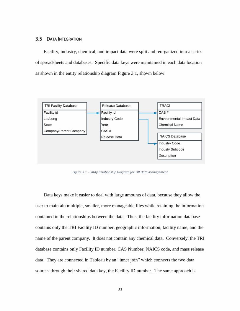
3.5 DATA INTEGRATION

Facility, industry, chemical, and impact data were split and reorganized into a series

of spreadsheets and databases. Specific data keys were maintained in each data location

as shown in the entity relationship diagram Figure 3.1, shown below.

Figure 3.1 - Entity Relationship Diagram for TRI Data Management

Data keys make it easier to deal with large amounts of data, because they allow the

user to maintain multiple, smaller, more manageable files while retaining the information

contained in the relationships between the data. Thus, the facility information database

contains only the TRI Facility ID number, geographic information, facility name, and the

name of the parent company. It does not contain any chemical data. Conversely, the TRI

database contains only Facility ID number, CAS Number, NAICS code, and mass release

data. They are connected in Tableau by an “inner join” which connects the two data

sources through their shared data key, the Facility ID number. The same approach is

32

taken with the TRACI data; it is linked only through the CAS Number which allows the

user to make complex calculations in Tableau without dealing with matrix multiplication

and enormous files.

3.6 TABLEAU WORKBOOK PUBLICATION

The workbooks involved in this thesis are available on Tableau’s public service.

Follow the link https://public.tableau.com/profile/ted2836 or visit public.tableau.com/en-

us/s and search “Ted Langlois”. The visualizations available will allow the user to toggle

through various subsets of TRI data, including the visualization used in the illustrative

examples that follow. By making these datasets publicly available, we hope to increase

the visibility of industry’s role in pollution and inspire groups to take control of their air,

water, and natural resources.

3.7 IMPROVEMENTS ON EXISTING TOOLS

While there is no doubt that existing TRI data visualization tools from EPA are

useful, they lack in certain areas including: availability of toxicity data, specific impact-

related information, and utility of data visualization. EPA’s work in data gathering and

development of tools for analysis has been extremely important for public access to

information, but now provides environmental data analysts the basis for a deeper

understanding of hazardous chemical releases and their environmental effects.

33

3.7.1 Toxicity Data

The EPA National Analysis uses mass-based reporting to determine which chemicals are

important to specific regions or industries. Figure 3.2 below shows the National Analysis results

for the top five chemicals (by mass) released to air and water in South Carolina in calendar year

2016, while Figure 3.3 shows an ecotoxicity-based analysis of data from the same year.

Figure 3.2 EPA National Analysis Fact Sheet, South Carolina 2016

Top Five Chemicals Released to Air and Water by Ecotoxicity SC, 2016

Air

*5.10% Other

Water

*5.08% Other

Figure 3.3 Tableau-Produced Ecotoxicity Analysis, South Carolina 2016

As is evident from the figures above, the National Analysis National Analysis

gives the user only releases by mass without any context of potential for harm. Based on

34

this analysis, one would begin investigations into chemicals such as methanol and

ammonia, which are commonly used in industry. An investigation based on TRACI

characterization factors and impact categories leads to a different conclusion. In the

TRACI method, ecotoxicty is measured in CTUe – ecological comparative toxicity units

– created to measure a chemical’s impact to aquatic organisms (Rosenbaum et al. 2008)

Through a comparison based on ecotoxicity, discussed in Appendix B, South Carolina

conservationists and lawmakers should be overwhelmingly concerned with metal

compounds containing zinc, and to a lesser extent, chromium, vanadium, and antimony.

The tool created here outperforms mass-based TRI analysis by connecting chemical data

to toxicity weighting schemes.

3.7.2 Impact-Based Data

TRACI improves the value of TRI data by defining the relationship between

chemical releases and midpoint impacts. RSEI leverages toxicity weights and dose data

to estimate risk to human health, but the method only aggregates risk from multiple

chemical sources into a single risk score. It provides no deeper data insights into the

types of environmental or human health damage may result in response to chemical

exposure. While the RSEI method is scientifically sound and aggregated risk scoring is

useful for comparison, it lacks the resolution required to analyze chemical releases for

their specific effects.

The tool outlined here provides measurable midpoint impacts in the form of

reference chemicals or toxicity units. Direct impact results can be traced back to their

corresponding chemical and the contribution of specific facilities to various impact

35

categories can be analyzed on a chemical-to-chemical basis. This is a clear improvement

on the EPA National Analysis in terms of toxicity and impact weighting and an

improvement on RSEI in terms of understanding chemical effects rather than risk alone.

3.7.3 Data Visualization

Data mapping, trends, and visualizations are important for conveying

environmentally relevant data. Both the National Analysis and RSEI tool have mapping

components and the ability to generate charts based on chemical, location, industry, and

in the case of RSEI, risk. Their interfaces are user friendly and easily accessible on the

web. However, the user is limited to the design provided by the EPA on its web pages.

For example, a user cannot view a side by side comparison of two states in the online

tool. The integration of the TRI dataset with Tableau offers the user the unique

opportunity to customize his or her data viewing experience. The user can download the

dataset in question and re-create or modify workbooks published online. Additionally,

Tableau provides features that allow the user to interact with graphs, charts, and maps, to

sort and expand information in ways that the EPA-produced maps cannot.

36

4 RESULTS: ILLUSTRATIVE EXAMPLES AND DATA INSIGHTS

The results from this data analysis are presented as a set of illustrative examples and

insights gleaned through data manipulation within the Tableau-based tool. The

illustrative examples here serve a few specific purposes. They highlight the tool’s

potential to improve legislative and policy choices, identify specific compounds or

industries that should be investigated as candidates for reduction activities, show

potential data issues or accounting errors, and help industry, government, and

communities prepare critical and vulnerable infrastructure in the event of natural

disasters. The goal is to provide examples of successful use of the TRI data tool to show

its ability to improve the usefulness of the TRI dataset.

4.1 ILLUSTRATIVE EXAMPLE 1: THE MONTREAL PROTOCOL

In 1987, the United States ratified the Montreal Protocol, in which 197 countries

agreed to phase out the production and use of chemicals that destroy ozone in the

stratosphere (Dept. of State 2016). These chemicals, which include chlorofluorocarbons

(CFCs) rise into the stratosphere where they interact with sunlight and create free

chlorine molecules which destroy ozone. (EPA “Basic Ozone Science” 2017). The

destruction of the ozone layer results in more intense sunlight and increases the potential

for the sun’s rays to cause skin cancer.

37

When experts laid out the policy in 1987, it was expected to result in the “avoidance

of more than 280 million cases of skin cancer, approximately 1.6 million skin cancer

deaths, and more than 45 million cases of cataracts in the United States alone by the end

of the century, with even greater benefits worldwide” (U.S. State Department 1987). The

global agreement represents an impressive example of international cooperation and its

positive effects. A NASA study published in early 2018 reported the first “direct proof”

that the CFC ban has caused a reduction in stratospheric ozone depletion (NASA 2018).

Using methods that measure directly the chemical composition of the ozone hole,

researchers were able to determine not only that ozone depletion is decreasing, but that a

lack of chlorine-containing chemicals is contributing.

Interestingly, CFCs are also extremely potent greenhouse gasses. They absorb

photons and vibrate similarly to carbon dioxide and contribute to global warming yet

have much greater potential to do so. The table below, from the Intergovernmental Panel

on Climate Change (IPPC) fourth assessment report, shows the global warming potential

of Montreal Protocol substance in units of kilograms carbon dioxide equivalent (IPPC

2007).

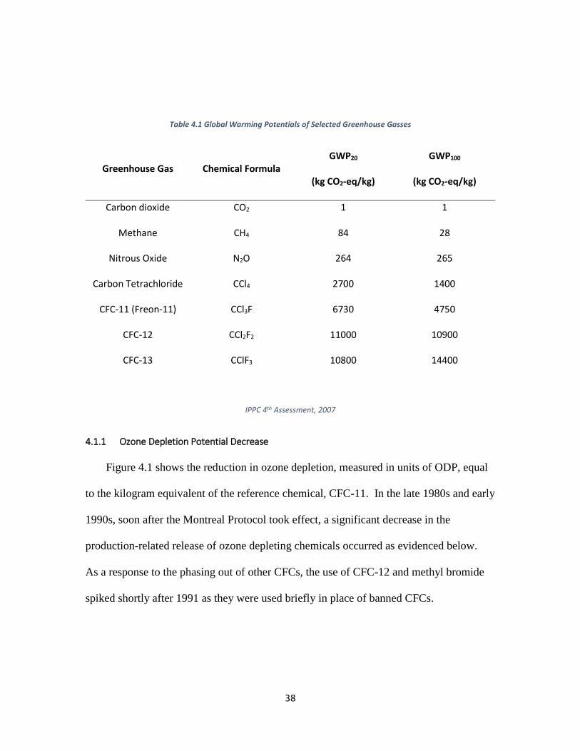
38

Table 4.1 Global Warming Potentials of Selected Greenhouse Gasses

Greenhouse Gas Chemical Formula GWP20

(kg CO2-eq/kg)

GWP100

(kg CO2-eq/kg)

Carbon dioxide CO2 1 1

Methane CH4 84 28

Nitrous Oxide N2O 264 265

Carbon Tetrachloride CCl4 2700 1400

CFC-11 (Freon-11) CCl3F 6730 4750

CFC-12 CCl2F2 11000 10900

CFC-13 CClF3 10800 14400

IPPC 4th Assessment, 2007

4.1.1 Ozone Depletion Potential Decrease

Figure 4.1 shows the reduction in ozone depletion, measured in units of ODP, equal

to the kilogram equivalent of the reference chemical, CFC-11. In the late 1980s and early

1990s, soon after the Montreal Protocol took effect, a significant decrease in the

production-related release of ozone depleting chemicals occurred as evidenced below.

As a response to the phasing out of other CFCs, the use of CFC-12 and methyl bromide

spiked shortly after 1991 as they were used briefly in place of banned CFCs.

39

Figure 4.1 Ozone Depleting TRI Chemicals 1986-2016

40

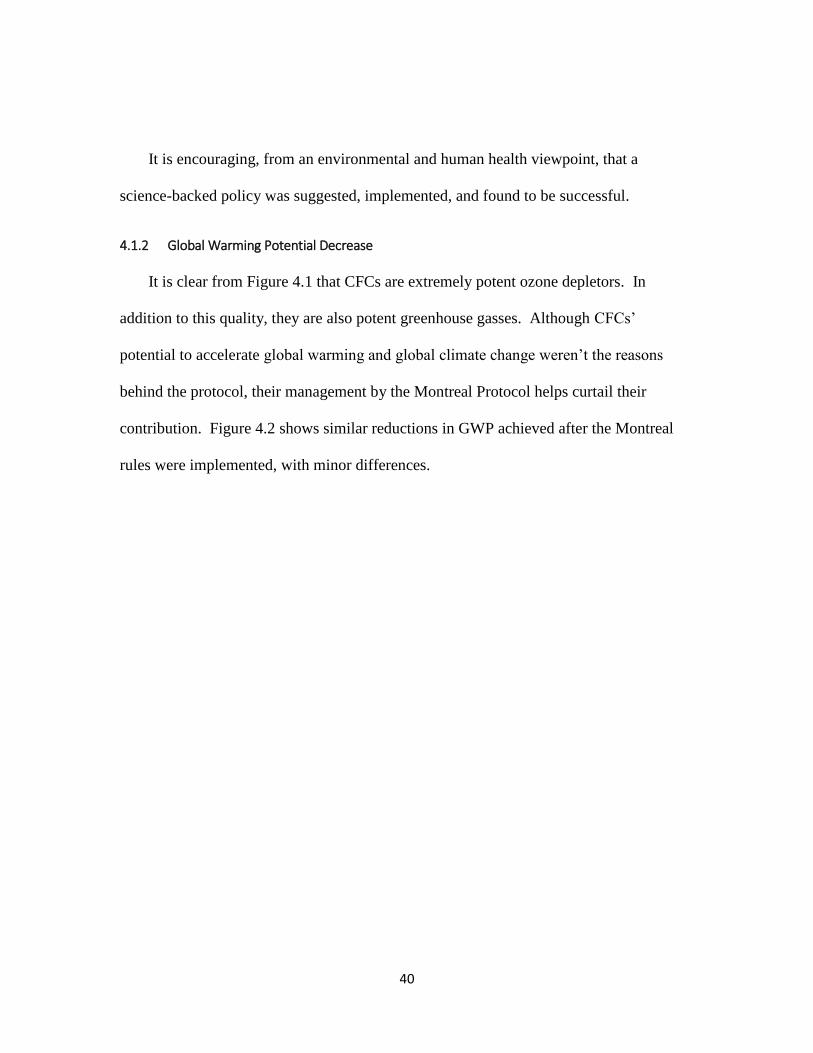
It is encouraging, from an environmental and human health viewpoint, that a

science-backed policy was suggested, implemented, and found to be successful.

4.1.2 Global Warming Potential Decrease

It is clear from Figure 4.1 that CFCs are extremely potent ozone depletors. In

addition to this quality, they are also potent greenhouse gasses. Although CFCs’

potential to accelerate global warming and global climate change weren’t the reasons

behind the protocol, their management by the Montreal Protocol helps curtail their

contribution. Figure 4.2 shows similar reductions in GWP achieved after the Montreal

rules were implemented, with minor differences.

41

Figure 4.2 TRI Greenhouse Gasses 1986-2016

42

It is interesting to note the differences in a chemical’s contribution to different

midpoint categories. CFC-12, for example, was added to the TRI list in 1991 and

contributes more to total global warming potential than it does to total ozone depletion

potential. The figure also highlights an important issue with the data involved in this

analysis. Due to the addition of CFC-12 in 1991, it appears that GWP increases briefly in

the year following. However, it is reasonable to assume that CFC-12 was being produced

and subsequently released in the United States prior to 1991 and in larger quantities.

Assuming this is true, it appears that GWP, and by extension ODP, decreased steadily

beginning in the late 1980s as a direct result of the Montreal Protocol.

4.2 ILLUSTRATIVE EXAMPLE 2: HYDROGEN CHLORIDE AIR RELEASES FROM ELECTRIC POWER

GENERATION

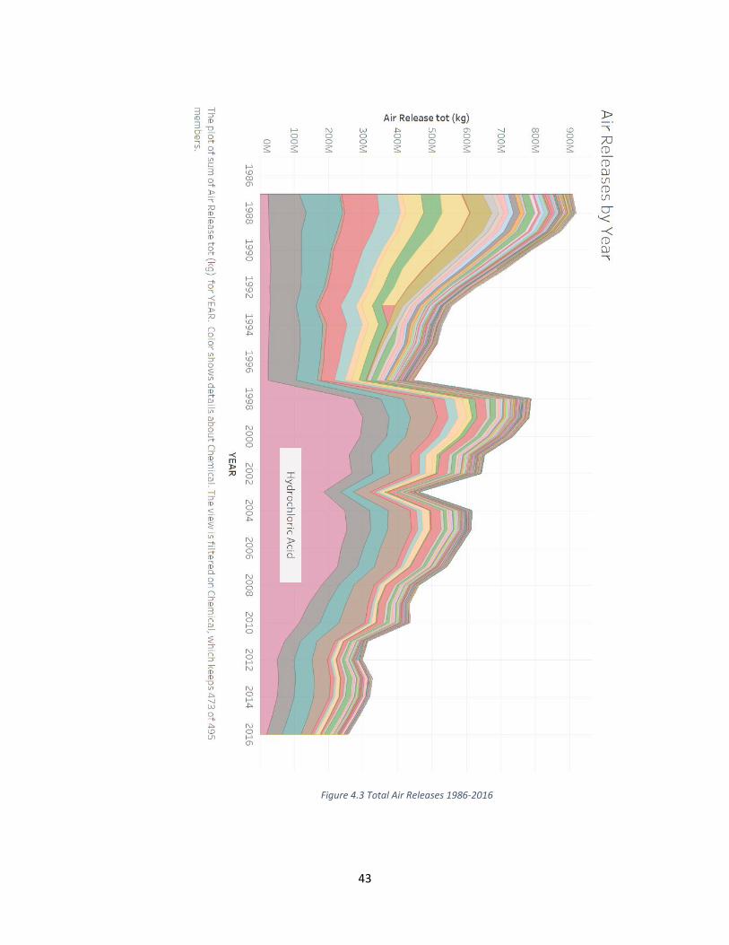
In identifying midpoint trends, it is useful to view air release trends more broadly. Since

the Montreal Protocol was effective in reducing ozone depleting chemicals, it may be

representative of broader trends in emissions reduction pursuant to the goal of the TRI.

Figure 4.3 includes all releases to air over time, with chemicals sorted by color and mass

released. While there is a general downward trend, there is a considerable increase after

1997 due to a large increase in reported emissions of hydrochloric acid.

43

Figure 4.3 Total Air Releases 1986-2016

44

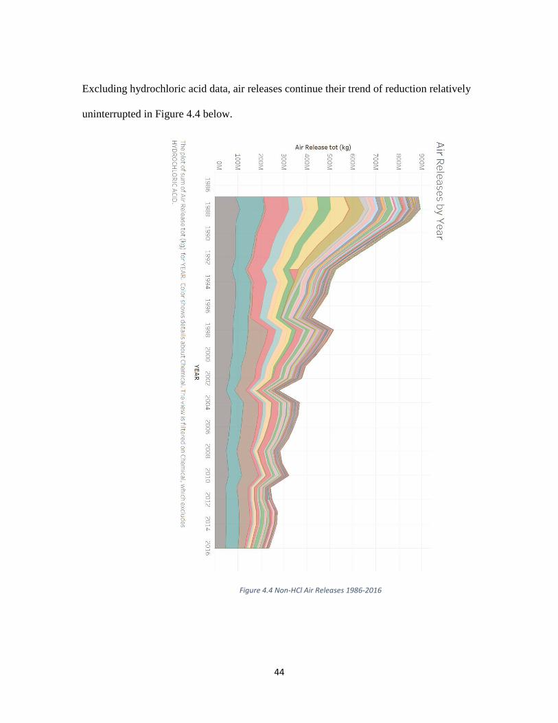
Excluding hydrochloric acid data, air releases continue their trend of reduction relatively

uninterrupted in Figure 4.4 below.

Figure 4.4 Non-HCl Air Releases 1986-2016

45

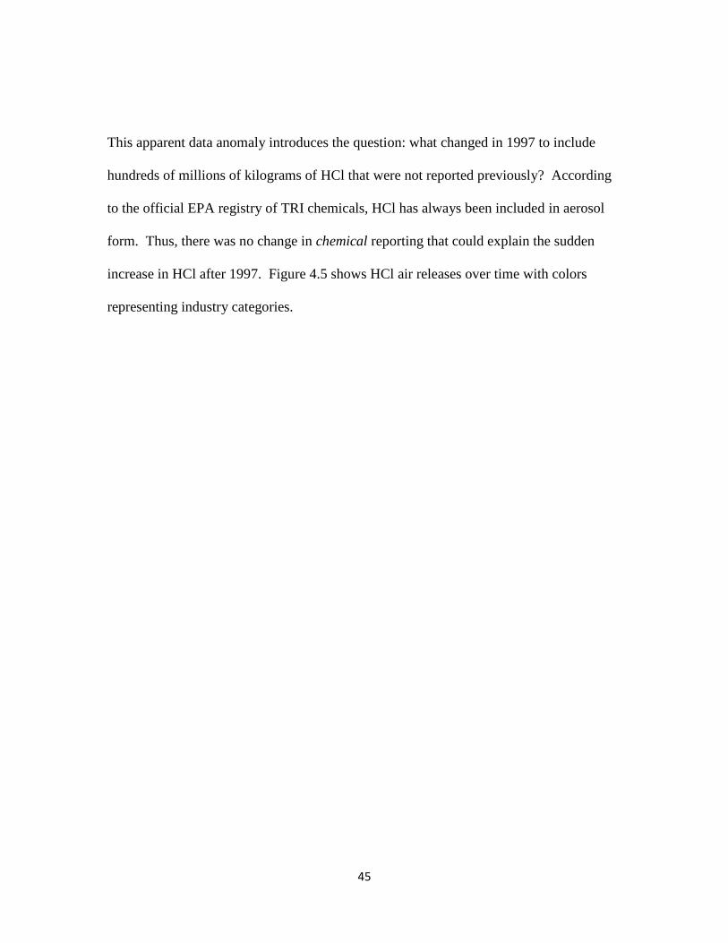
This apparent data anomaly introduces the question: what changed in 1997 to include

hundreds of millions of kilograms of HCl that were not reported previously? According

to the official EPA registry of TRI chemicals, HCl has always been included in aerosol

form. Thus, there was no change in chemical reporting that could explain the sudden

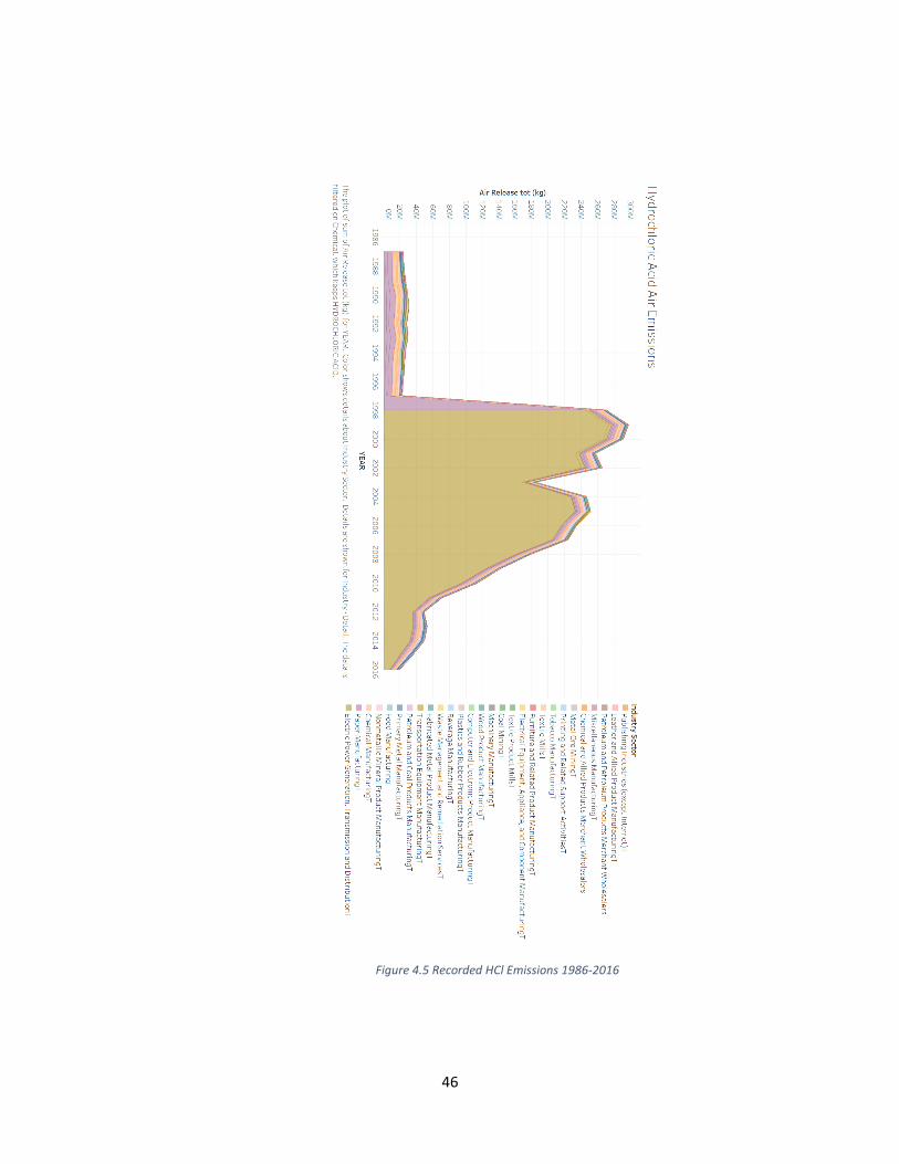
increase in HCl after 1997. Figure 4.5 shows HCl air releases over time with colors

representing industry categories.

46

Figure 4.5 Recorded HCl Emissions 1986-2016

47

The figure shows that almost all the HCl reported after 1997 can be attributed to a

single industry sector: Electric Power Generation, Transmission and Distribution. This

industry did not appear in the data before the year in question. For the reporting year

1998, and each year after, the EPA required power plants that burn coal or oil to report

their chemical uses to TRI, based on a projection that suggested that “the magnitude of

electric utility industry releases will surpass those of the manufacturing industries which

currently report to TRI” (Rubin, 1999). Thus, emissions data for HCl, which was

previously unreported from the power generation industry suddenly appears in the record.

The addition of an industry sector and its effect on emissions data is problematic. In

some ways it is analogous to finding a ten-dollar bill in one’s pocket. One is glad to have

the money, but one also must recognize that he or she must have lost ten dollars at some

point. Differences in reporting methods and requirements lead to important questions. If

all industries are not required to report their emissions, is there much point to tracking

them? Can we earnestly tout our chemical use reductions without a complete set of data?

While the data is disappointingly incomplete prior to 1998, the data since then is quite

illuminating.

HCl emissions peak in the late 1990s and early 2000s, as evidenced by Figure 4.5.

However, there is a roughly one-third reduction in total releases between 1999 and 2003,

followed by another increase before more serious reductions begin to occur around 2007.

These reductions were a direct result of changes in federal legislation. As a Hazardous

Air Pollutant (HAP), HCl is regulated by National Emission Standards for Hazardous Air

Pollutants (NESHAP). This standard sets limits for “production facilities” that are a

48

major source of a specific HAP. In 2001, a rule change was proposed to limit the release

of HCl from industrial facilities (Federal Register 2001). In response to the proposal, it

appears that industrial facilities preemptively began to reduce HCl, leading to a local

minimum in 2003. Despite this new rule, HCl releases rebounded until 2006 when, after

public comment, the EPA finalized further amendments to NESHA, and required

facilities with “major sources to meet HAP emission standards and implement work

practice standards that reflect the application of maximum achievable control

technology” and included clarifications on “applicability provisions, emissions standards,

and testing” (National Register). Again, despite a lack of early data, the hydrochloric

acid rule seems to be another example of positive outcomes from both the availability of

toxic release data and government intervention for the purposes of safeguarding human

health.

4.3 ILLUSTRATIVE EXAMPLE 3: NATURAL DISASTER PLANNING AND RESILIENCE IN THE

AFTERMATH OF HURRICANE HARVEY

In late August of 2017, Category 4 hurricane Harvey made landfall on the Gulf

Coast of Texas (CNN 2017). The storm broke the United States record for rainfall from a

single storm and flooded much of the southeastern part of the state. A unique

combination of geographic, economic, and meteorological factors contributed to the

severity of the flooding and its potential effects on the environment and human health.

First, Houston, America’s fourth largest city, has grown 23% in population since 2001

49

and its metropolitan area measures 9,000 square miles. Urban sprawl has resulted in the

construction of more impermeable surfaces such as paved streets, parking lots, and

sidewalks, which reduces an area’s ability to absorb water and increases the severity of

flooding events.

Second, the low-lying city is home to numerous petroleum companies, refineries,

and chemical manufacturers. These chemical consumers and producers contribute

significantly to the TRI under normal operation. During natural disaster events, they

become infrastructure critical to keep intact. The accidental release of many of the

chemicals stored and used in these facilities could cause major damage to ecosystems and

human health.

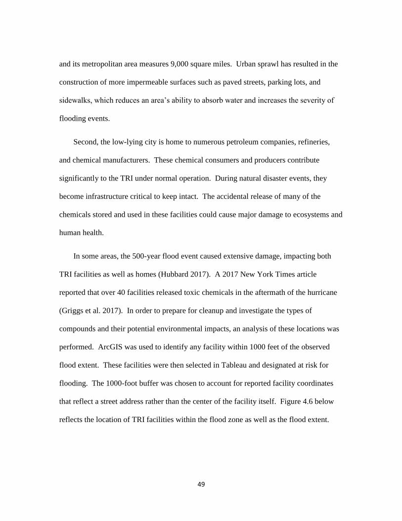
In some areas, the 500-year flood event caused extensive damage, impacting both

TRI facilities as well as homes (Hubbard 2017). A 2017 New York Times article

reported that over 40 facilities released toxic chemicals in the aftermath of the hurricane

(Griggs et al. 2017). In order to prepare for cleanup and investigate the types of

compounds and their potential environmental impacts, an analysis of these locations was

performed. ArcGIS was used to identify any facility within 1000 feet of the observed

flood extent. These facilities were then selected in Tableau and designated at risk for

flooding. The 1000-foot buffer was chosen to account for reported facility coordinates

that reflect a street address rather than the center of the facility itself. Figure 4.6 below

reflects the location of TRI facilities within the flood zone as well as the flood extent.

50

Figure 4.6 Map of Observed Flood Extent with TRI Facilities

To prepare for a flood event such as Harvey or to predict what classes of chemicals

may be present in soil and groundwater after release, it is important to create an inventory

of chemicals present in vulnerable facilities. The Tableau tool can be used to assess types

of chemical and their potential ecotoxicity effects in water. Figure 4.7 shows the top 10

chemical processors in the affected area by mass reported to TRI. It is useful to note that

the data available is the total mass of compound “released” in some capacity during

calendar year 2016. Here, “total releases” refer to any chemical processed according to

51

the P2 hierarchy: energy recover, recycling, treatment, and release to the environment.

At any given time, the chemicals presented in this figure are certainly not present in their

respective facilities, but it can be reasonably assumed that some fraction of each of them

is present at a given moment. Additionally, without access to the 2017 data, an accurate

sum of specific compounds cannot be provided, 2016 data must be used as a surrogate.

52

Figure 4.7 Chemical Inventory for Potentially Flooded Texas TRI Facilities – Top 10 by Mass

Figure 4.8 Chemical Inventory for Potentially Flooded Texas TRI Facilities – Top 10 by Ecotoxicity

53

The chemicals present in these ten facilities are commonly consumed in large

quantities by chemical manufacturers. They appear in the TRI National Analysis in large

quantities. However, while it is useful to understand which chemicals are used in Texas

facilities and in what amount, the compounds present here may not be the most toxic

chemicals present in the Gulf Coast region. Figure 4.8 lists the top 10 facilities based on

potential to cause ecosystem damage in a major flood event. The unit for ecotoxicity

applied through TRACI is CTUe, which is proportional to the potentially affected fraction

of species in an ecosystem (Rosenbaum 2008). It is important to note here that to cause

the damage mentioned, the facility would have to become completely flooded and lose a

complete years’ worth of chemical inventory. Still, it is useful to understand potential

hazards associated with natural disaster events.

By mass, none of the top 10 chemical processors have the potential to be the top 10

sources of ecotoxicity in a flood event. This shows the role toxicity plays in assessing

potential environmental damage, and the usefulness of an LCIA tool to weight chemicals

based on their impacts. Disaster awareness and planning based on mass would severely

undervalue the facilities that could be a greater risk to human and environmental health in

the event of an incident.

54

5 CONCLUSIONS AND FUTURE WORK

5.1 A TOOL FOR INDUSTRY, GOVERNMENT, AND COMMUNITIES

The online tool produced by this thesis is meant to show the potential for data

visualization tools like Tableau, combined with toxicity weighting schemes, to improve

our understanding of toxic releases and their sources. In the age of big data and real-time

analytics, more possibilities exist for improvement and decision-making built around the

protection of human health and the environment. The thought behind the TRI program

when it was announced in 1986 was to create unprecedented public access to data that

was previously unreachable. Today, we have even greater access and more powerful

tools to analyze that data.

5.2 A MODEL FOR BETTER DATA ANALYSIS

As a visualization tool, Tableau is incredibly useful and intuitive. It is not the only

tool available for data analysts, and perhaps not even the most powerful. However, the

model presented here – data collection, compilation, combination with an outside

scientific methodology – can be repeated with a great number of disparate data sets. For

example, the same methods could be applied to an analysis of the National Emissions

Inventory, a separate, EPA-produced set of environmental data, or with Canada’s

National Pollution Release Inventory. Coal and natural gas fired power plants

monitoring NOx, SOx, mercury, and particulate matter could report in real time to a data-

55

gathering system. Repeating the process shown above, the public could receive real-time

information on the environmental and health hazards that power plant emissions cause.

As mentioned in section 2.8, other impact assessment and toxicity weighting tools

exist. The author would recommend that future work expand the use of the TRACI tool

to include other LCIA packages such as ecoindicator99 (2000) or ReCiPe (2016). The

integration of these methodologies with TRACI and the Tableau-based tool could

confirm or challenge the results of this thesis and lead to more nuanced and rich

understandings of the TRI dataset.

On the subject of repeating or improving on this research, the author recommends

that future TRI dataset users download EPA’s yearly .csv files and import them directly

into an SQL database rather than combining the files first in another format.

Additionally, it would be useful for EPA to provide the raw data in a long data format, in

a single database, directly to users. This would effectively remove the necessity of

downloading each year’s data individually and allow data analysis to begin without much

work by the end user.

However it is used, we have access to more environmentally relevant information

than at any point in history. The responsibility is on us to use data to protect our

resources and the quality of our environment.

56

57

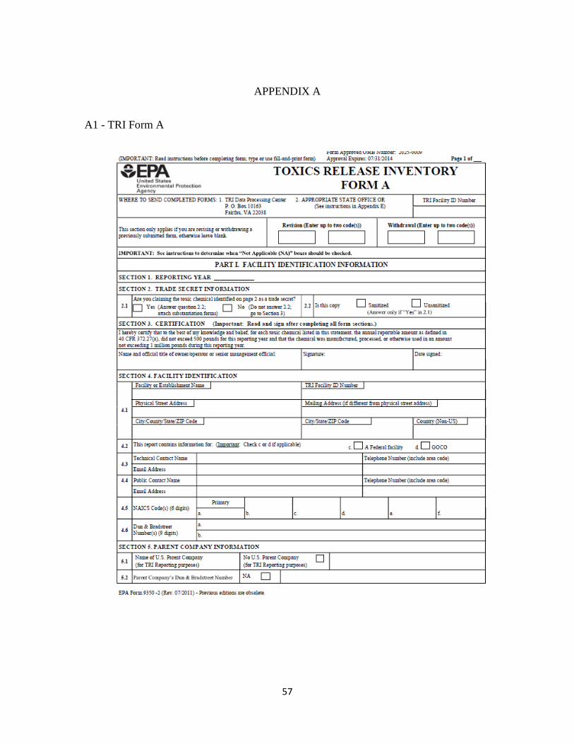
APPENDIX A

A1 - TRI Form A

58

59

A2 – TRI Form R

60

61

62

63

64

APPENDIX B

SUBMITTED TO THE SOUTH CAROLINA WATER RESOURCES JOURNAL

Visualizing Relative Potentials for Aquatic Ecosystem Toxicity

Using the EPA Toxics Release Inventory

and Life Cycle Assessment Methods

Theodore Langlois, Michael Carbajales-Dale, Elizabeth Carraway

AUTHORS: Department of Environmental Engineering and Earth Sciences, Clemson University, 342 Computer Court,

Anderson, SC 29625, USA.

Abstract. As a result of the 1986 Emergency

Planning and Community Right-to-Know Act,

the U.S. EPA Toxic Release Inventory (TRI)

has been available since 1987 as a record of

industrial releases of toxic chemicals.

Combining TRI data with estimates of relative

toxicity of these chemicals to aquatic systems

increases the utility of the database by

providing a common basis for comparison. TRI

reports masses of approximately 170 chemicals

or chemical classes released to water, air, and

soil. The Tool for Reduction and Assessment of

Chemicals and Other Environmental Impacts

(TRACI) is a database of Characterization

Factors (CFs) developed from chemical studies

and environmental transport models to assess

environmental impacts with respect to a

reference compound or unit of toxicity. Using

Life Cycle Assessment (LCA) techniques,

these data have been combined to based tools to

estimate comparative aquatic ecosystem

toxicity in comparative toxicity units (CTUe).

The visualization software Tableau was used to

generate representations of the preliminary

results in this communication. The major

potential sources of aquatic toxicity have been

identified for South Carolina by industry type

and by year over the period 1987-2016. The

possibility of toxicity from releases of zinc

compounds from power generation and pulp

and paper mills far exceeds all other sources.

Zinc compounds are seen to dominate the

annual CTUe over the full time period 1987-

2016 with periodic decreases reflecting

economic factors. Locations of releases are

generally seen to occur near the major

manufacturing and urban areas in the state.

Trends in total CTUe in South Carolina over

1987-2016 compared to the U.S. as a whole

reveal comparative toxic effects of total

releases in the state generally track the nation

except for periods in the late 1990s and in the

mid-2000s when toxicity was down nationally.

INTRODUCTION

While the growth of the manufacturing

sector is beneficial to many aspects of South

Carolina’s economy, there may be unintended,

negative consequences for the state’s natural

65

resources. Direct releases of hazardous

chemicals by industrial facilities to South

Carolina waterways can harm species

important for ecosystem health, biodiversity,

and recreation. The U.S. EPA Toxics Release

Inventory (TRI) tracks releases of 692

chemicals and chemical classes, but lacks

specific data relevant to toxicity and

environmental harm. Combining chemical

evaluation methods such as those developed

within the framework of Life Cycle Assessment

(LCA) with TRI data can fill that gap. This

communication presents initial results obtained

using TRI data for freshwater in South Carolina

and LCA methodologies. Developments using

LCA methodologies, combined with the data

visualization tool Tableau, provide additional

and more nuanced information about the

potential for environmental damage associated

with industrial releases. The resulting tool

provides a novel perspective for viewing TRI

data. By utilizing the best available toxicity

data and a powerful visualization tool, complex

relationships between chemicals and the

environment become more accessible to the

public. The results enable a better

understanding the potential impacts of

manufacturing in the state of South Carolina

and demonstrate the utility of data visualization

techniques.

PROJECT DESCRIPTION

In response to the December 1984 industrial

disaster at a Union Carbide plant in Bhopal,

India which released approximately 40 tonnes

of methyl isocyanate (CH3NCO) gas, and

smaller-scale industrial accidents in the United

States, Congress passed the 1986 Emergency

Planning and Community Right-to-Know Act

(Broughton 2005, Koehler 2007). The law

addressed the potential for incidents that could

affect human health in areas surrounding

chemical or industrial plants. Section 313 of

this statue charged the Environmental

Protection Agency with creating a list of

facilities and their yearly releases of hazardous

chemicals, the result being the Toxics Release

Inventory. The EPA maintains a list of toxic

chemicals and thresholds that, if exceeded by a

facility, must be reported. The resulting

database offers individuals and communities

yearly, itemized reports of industrial activities

and hazardous chemicals that may impact their

neighborhoods. As legislation, TRI initiated a

new way of regulating industry; instead of an

agency enforcing limits, it provides an

information network which private citizens and

interest groups can use to exert pressure on

polluters until they reduce toxic waste to a level

the public deems acceptable (Fung and

O’Rourke 2000). It is important to note that

TRI does not track illegal releases, rather, it

accounts for permitted releases associated with

industrial processes. The program is generally

agreed to be quite successful. From 1988, the

second year of the program, to 1995 the total

amount of toxic chemicals released or

transferred decreased by about 45% (US EPA

1995).

While serving as a valuable tool for

communities, the TRI does not include toxicity

data within the database. Available data are

presented as releases to water, air, and land by

pound of chemical. Thus, a user can compare

releases of mercury compounds to lead

compounds only by mass, with no indication of

the potential for harm. More comprehensive

analysis and models are needed to assess

potential risk or damage to human and

ecosystem health. To some degree, EPA has

remedied this knowledge gap in annual

publications. Along with the TRI National

Analysis, a document analyzing yearly release

trends, the agency has created a risk-based

model, the Risk-Screening Environmental

Indicators (RSEI) which is available online for

public use. The RSEI model assigns toxicity

weights to chemicals that affect human health.

While this model provides a measure of

66

toxicity, it is a risk-based model focused solely

on human health.

Additionally, the EPA in 2016 released a

visualization tool to present TRI data and

provide outreach for its Pollution Prevention

(P2) program (Gaona and Kohn 2016). The tool

uses visualization and mapping software Qlik

to produce useful stories valuable to the public.

Although useful for communicating risk to the

public, this specific tool, like the TRI itself,

conveys only pounds of toxic waste managed.

Life Cycle Assessment (LCA) is a tool

generally reserved for evaluating the cradle-to-

grave impacts of a product or system, however,

LCA provides tools useful for analysis of

environmental impacts on a local, statewide,

and national scale. LCA is comprised of four

phases: goal and scope definition, inventory

analysis, impact assessment, and interpretation.

In the inventory phase, elemental flows are

tracked into and out of a product system. Raw

materials, water, and energy may enter the

boundaries of this system, while a final product

and associated emissions exit the boundary.

While the TRI does not track products, it

represents an inventory of chemical by-

products from manufacturing. In the impact

assessment phase, an LCA practitioner uses

inventory results to determine what type of

impact is associated with their release to the

environment.

These impacts belong to either midpoint or

endpoint categories. Midpoint impacts are

measurables that are directly influenced by

chemical releases. For example, global

warming potential (GWP) is a midpoint

category that greenhouse gasses directly

impact, while climate change is the endpoint

impact related to GWP. Multiple midpoint

impacts, such as aquatic ecotoxicity, acidity,

and eutrophication impact the ecosystem

quality endpoint. Several models may be used

to directly relate chemical releases into the

environment with midpoint impacts. One such

model, the Tool for Reduction and Assessment

of Chemicals and Other Environmental Impacts

(TRACI), uses Characterization Factors (CFs)

based on chemical studies and environmental

transport models, to assess environmental

impacts with respect to a reference compound

or unit of toxicity (EPA 2012).

METHODS

In this analysis, direct-to-water releases are

converted to toxicity values using their CFs

found in the TRACI database. The final LCA

phase, interpretation, is done through analysis

and visualization using Tableau software.

TRI and TRACI data were downloaded from

the EPA website, compiled into Microsoft

Access databases, and imported into Tableau

data visualization software for analysis (EPA

2018). The process is outlined in Figure 1.

Figure 1. Data generation and visualization

methodology.

Ecosystem toxicity, referred to in TRACI as

ecotoxicity, is measured in comparative

toxicity units (CTUe), which are proportional to

estimates of potentially affected fraction of

species (PAF), integrated over time and

volume, per unit mass of a chemical emitted

(USEtox 2010). This calculation, shown below,

allows different chemicals to be compared in

terms of their potential to harm species within

an ecosystem.

67

The mass of chemical released according to the

TRI database is W, measured in kilograms. The

characterization factor CF, measured in

CTUe/kg, is the measure of toxicity associated

with each chemical in the TRACI database.

When multiplied together, using a tableau data

join and in-program calculation, the product is

a comparative toxicity value for each year and

reporting location for each chemical or

chemical class. The comparative nature of this

toxicity measure must be stressed; the CTUe is

not a measure of species affected by a chemical,

rather it represents a method of comparing

relative toxicity across a wide range of

conditions and releases.

The TRACI database includes multiple CFs

for different modes of release: to air (urban or

rural), water (fresh or marine), and land

(agricultural or natural soil). Several

assumptions must be made for consistent

results. First, we assume that all chemical

releases are made to freshwater. Second, since

TRI data groups certain metal compounds

together and TRACI does not, a proxy

compound must be chosen to represent a group

of compounds. The RSEI methodology

document, produced by EPA, states that these

compound categories are assumed to be metals

in their most toxic form (US EPA 2018). Thus,

the TRI category for “Copper Compounds” is

associated with the TRACI chemical “Copper

(II)”.

RESULTS

Figure 2 presents the comparative toxicity (in

millions of CTUe) for total TRI releases to

water in South Carolina between 1987 and

2016 grouped by industry sectors. A few

industries and chemicals have dominated

ecotoxicity to South Carolina’s waterways over

the past 30 years. It is clear that zinc

compounds consistently present the largest

ecosystem risk, especially from fossil fuel

generation and paper and pulp mills sectors.

Four of the top ten largest sources are related to

paper or pulp manufacturing. Other

significantly toxic releases include copper,

vanadium, cobalt, and antimony compounds.

Figure 3 shows the annual trend in

ecotoxicity risks over the history of TRI data

collection, with time on the X-axis and

ecotoxicity measured in CTUe on the Y-axis.

Vanadium compounds were added to the TRI

list in 2000, adding to the overall yearly

toxicity. Despite a general increase in

production efficiency in the US, the level of

toxicity released to South Carolina water bodies

increased in the late 1990s and experienced

another increase in the mid-2000s, most likely

to an overall increase in manufacturing in the

state. However, releases decreased sharply in

the late 2000s, due to economic recession,

which is reflected in this data (Koh et al. 2016).

Figure 4 maps locations of cumulative toxic

chemical releases to South Carolina waters over

1987-2016. The distribution of TRI releases is

seen to align with major manufacturing areas in

the state. There are concentrations in the

Spartanburg-Greenville area, the Charlotte

Metro area, Georgetown, and Charleston. Many

plants sit on fresh water bodies used for

recreation and often drinking water supply.

Figure 5 presents a comparison of annual

variability of the comparative ecotoxicity of

TRI releases in South Carolina and the U.S. as

a whole. Interestingly, the trends in ecotoxicity

to not directly correlate between South Carolina

and the rest of the United States. While

ecotoxicity in the early years of TRI declined in

the United States, it remained relatively low

and stable in South Carolina. However, if

68

increases in toxic releases can be attributed to

increases in manufacturing, it seems that South

Carolina was ahead of the rest of the country in

its increase in the late 1990s and increased

again in the mid-2000s while toxicity was down

nationally. Finally, the state was consistent with

the rest of the country with respect to the

decline in operation and subsequent toxic

releases after the financial crisis of 2008. While

release of hazardous materials can be tied to

economic growth, especially for the

manufacturing sector, it is of course not a

desirable outcome. As South Carolina

continues to grow its economy through

industry, companies and private citizens should

closely monitor environmental impacts of

hazardous chemical release.

DISCUSSION

The apparent variability in toxicity levels

indicates potential problems with using TRI as

a marker for gains or losses in environmental

protection. First, the nature of the reporting

mechanisms places relatively little importance

on accuracy. It is estimated that in its first year,

10,000 out of 30,000 facilities required to

comply with the program failed to do so and in

any given year, only 3% of facilities are

investigated by EPA (Wolf 1996). Second, the

sitting EPA administration has the power to add

and remove chemicals on a year-by-year basis.

This means that the chemical list from 1987

differs significantly from the 2016 list. Third,

chemicals can change reporting categories. In

one year, a chemical release or method of

treatment may be listed in different category.

This creates a phantom or paper reduction, in

which appears as a decrease in trends, but does

not in fact correspond to a physical reduction

(Natan and Miller 1998). Despite reporting

errors, changing categories, or addition and

removal of chemicals, the analysis of TRI using

Life Cycle Impact Assessment methods proves

to be a powerful tool for identifying data trends.

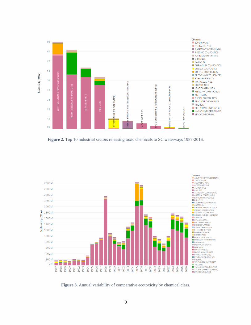
0

Figure 2. Top 10 industrial sectors releasing toxic chemicals to SC waterways 1987-2016.

Figure 3. Annual variability of comparative ecotoxicity by chemical class.

1

Figure 4. Comparative ecotoxicity of

1987-2016 releases from South

Carolina facilities.

Figure 5. South Carolina and U.S. trends

in comparative ecotoxicity 1987-2016.

2

REFERENCES

Baayen, Harry. "Eco-indicator 99 Manual for Designers." 2000. <https://www.pre-

sustainability.com/download/EI99_Manual.pdf>.

Bajak, Frank, and Lise Olsen. "Hurricane Harvey's Toxic Impact Deeper than Public

Told." Houston Chronicle March 23 2018.

Bare, Jane. "TRACI 2.0: The Tool for the Reduction and Assessment of Chemical and

Other Environmental Impacts 2.0." Clean Technologies and Environmental Policy

13.5 (2011): 687.

Bouwes, N., and S. Hassur. Toxics Release Inventory Relative Risk-Based

Environmental Indicators Methodology. Bethesda, MD: Office of Pollution

Prevention and Toxics, U.S. Environmental Protection Agency, 1997.

Bowsher, Charles A. Toxic Chemicals: EPA's Toxic Release Inventory is Useful but can

be Improved. United States General Accounting Office, 1991.

Broughton, Edward. "The Bhopal Disaster and its Aftermath: A Review." Environmental

Health 4.6 (2005).

Dunklin, Reese. "Agency: Texas Chemical Plant Unprepared for Harvey Floods."

Associated Press May 24 2018.

Environmental Protection Agency. Aermod., 2005.

---. "Basic Ozone Layer Science." 2017. <https://www.epa.gov/ozone-layer-

protection/basic-ozone-layer-science>.

---. "Clinton-Gore Administration Announces First-Ever Data on Toxic Emissions from

Seven Major Industrial Sectors." 2000.

---. "Hazardous Waste Recycling." 2017. <https://www.epa.gov/hw/hazardous-waste-

recycling>.

---. "Introduction to the 2016 TRI National Analysis." 2018.

<https://www.epa.gov/trinationalanalysis/introduction-2016-tri-national-analysis>.

---. "Pollution Prevention (P2)." 2018. <https://www.epa.gov/p2>.

3

---. Toxics Release Inventory - TRI Form R and Form A Toxic Chemical Release

Reporting

Information Collection Request Supporting Statement., 2011.

Fung, Archon, and Dara O'Rourke. "Reinventing Environmental Regulation from the

Grassroots Up: Explaining the Success of the Toxics Release Inventory." Journal of

Environmental Management 25.2 (2000): 115.

Gaona, Sandra, and Jeff Kohn. Using the Visualization Software Qlik for TRI Data

Presentation and P2 Outreach. Washington, DC: Environmental Protection Agency,

2016.

Glossary of Environment Statistics, Studies in Methods, Series F, no. 67, United Nations,

New York, 1997.

Graham, Mary, and Catherine Miller. "Disclosure of Toxic Releases in the United

States." Environment: Science and Policy for Sustainable Development 43.8 (2001):

8.

Intergovernmental Panel on Climate Change. "Direct Global Warming Potentials." 2007.

<https://www.ipcc.ch/publications_and_data/ar4/wg1/en/ch2s2-10-2.html>.

Johnson, Stephen L. National Emission Standards for Hazardous Air Pollutants:

Hydrochloric Acid Production. 42 U.S.C. 7401 et seq. ed., 2006.

Koehler, Dinah A., and John D. Spengler. "The Toxic Release Inventory: Fact Or

Fiction? A Case Study of the Primary Aluminum Industry." Journal of

Environmental Management 85 (2007): 296.

Lim, Seong-Rin, Lam, Carl W., Schoenung, Julie M. "Priority Screening of Toxic

Chemicals and Industry Sectors Int He U.S. Toxics Release Inventory: A

Comparison of the Life Cycle Impact-Based and Risk-Based Assessment Tools

Developed by U.S. EPA." Journal of Environmental Management 92 (2011): 2235.

Natan, Thomas E., and Catherine G. Miller. "Are Toxics Release Inventory Reductions

Real?" Environmental Science and Technology 3.8 (1998): 368A.

Netherlands National Institute for Public Health and the Evironment. "ReCiPe." 2011.

<https://www.rivm.nl/en/Topics/L/Life_Cycle_Assessment_LCA/ReCiPe>.

Rosenbaum, Ralph K. et al. "USEtox - the UNEP-SETAC Toxicity Model:

Recommended Characterisation Factors for Human Toxicity and Freshwater

Ecotoxicity in Life Cycle Impact Assessment." International Journal of Life Cycle

Assessment (2008).

4

Rubin, Edward S. "Toxic Releases from Power Plants." Environmental Science and

Technology 33.18 (1999): 3062.

Samenow, Jason. "Harvey is a 1,000-Year Flood Event Unprecedented in Scale." The

Washington Post August 31 2017.

Strahan, Susan E., and Anne R. Douglass. "Decline in Antarctic Ozone Depletion and

Lower Stratospheric Chrlorine Determed from Aura Microwave Limb Sounder

Observations." Geophysical Research Letters 45.1 (2018): 382.

Tabuchi, H., et al. "Floods are Getting Worse, and 2,500 Chemical Sites Lie in the

Water's Path." The New York Times February 6 2018.

Toffel, Michael W., and Julian D. Marshall. "Improving Environmental Performance

Assessment: A Comparative Analysis of Weighting Methods used to Evaluate

Chemical Release Inventories." Journal of Industrial Ecology 8.1 (2004): 143.

Truhaut, R. "Ecotoxicology: Objectives, Principles and Perspectives." Ecotoxicology and

Environmental Safety 1.2 (1977): 151.

U.S. Department of State. "The Montreal Protocol on Substances That Deplete the Ozone

Layer." 2016. <https://www.state.gov/e/oes/eqt/chemicalpollution/83007.htm>.

"What is EPCRA." 2018. <https://www.epa.gov/epcra/what-epcra>.

Wolf, Marc Andree, et al. "The International Reference Life Cycle Data System

Handbook." (2012).

Wolf, Sydney M. "Fear and Loathing about the Public Right to Know: The Surprising

Success of the Emergency Planning and Community Right-to-Know Act." Journal of

Land Use & environmental Law 11.2 (1996): 217.