A Volume Integral Equation Method for the Direct/Inverse

1

A Volume Integral Equation Method for the Direct/Inverse Problem in Elastic Wave

Scattering Phenomena

Terumi Touhei Department of Civil Engineering, Tokyo University of Science,

Japan

1. Introduction

The analysis of elastic wave propagation and scattering is an important issue in fields such as earthquake engineering, nondestructive testing, and exploration for energy resources. Since the 1980s, the boundary integral equation method has played an important role in the analysis of both forward and inverse scattering problems. For example, Colton and Kress (1998) presented a survey of a vast number of articles on forward and inverse scattering analyses. They also presented integral equation methods for acoustic and electromagnetic wave propagation, based on the theory of operators (1983 and 1998). Recently, Guzina, Fata and Bonnet (2003), Fata and Guzina (2004), and Guzina and Chikichev (2007) have dealt with inverse scattering problems in elastodynamics. The type of volume integral equation known as the Lippmann–Schwinger equation (Colton & Kress, 1998) has been an efficient tool for theoretical investigation in the field of quantum mechanics (see, for example, Ikebe, 1960). Several applications of the volume integral equation to scattering analysis for classical mechanics have also appeared. For example, Hudson and Heritage (1981) used the Born approximation of the solution of the volume integral equation obtained from the background structure of the wave field for the seismic scattering problem. Recently, Zaeytijd, Bogaert, and Franchois (2008) presented the MLFMA-FFT method for analyzing electro-magnetic waves, and Yang, Abubaker, van den Berg et al. (2008) used a CG-FFT approach to solve elastic scattering problems. These methods were used to establish a fast algorithm to solve the volume integral equation via a Fast Fourier transform, which is used for efficient calculation of the convolution integral. In this chapter, another method for the volume integral equation is presented for the direct forward and inverse elastic wave scattering problems for 3-D elastic full space. The starting point of the analysis is the volume integral equation in the wavenumber domain, which includes the operators of the Fourier integral and its inverse transforms. This starting point yields a different method from previous approaches (for example, Yang et al., 2008). By replacing these operators with discrete Fourier transforms, the volume integral equation in the wavenumber domain can be treated as a Fredholm equation of the 2nd kind with a non-Hermitian operator on a finite dimensional vector space, which is to be solved by the Krylov subspace iterative scheme (Touhei et al, 2009). As a result, the derivation of the coefficient matrix for the volume integral equation is not necessary. Furthermore, by means of the Fast

Source: Wave Propagation in Materials for Modern Applications, Book edited by: Andrey Petrin, ISBN 978-953-7619-65-7, pp. 526, January 2010, INTECH, Croatia, downloaded from SCIYO.COM

www.intechopen.com

Wave Propagation in Materials for Modern Applications

2

Fourier transform, a fast method for the volume integral equation can be established. The method itself can be extended to the scattering problem for a 3-D elastic half space (Touhei, 2009). This chapter also presents the possibility of the volume integral equation method for 3-D elastic half space by constructing a generalized Fourier transform for the half space. An important property of the volume integral equation in the wavenumber domain is that it separates the scattered wave field from the fluctuation of the medium. This property yields the possibility of inverse scattering analysis. There are several methods for inverse scattering analysis that make use of the volume integral equation (for example, Kleinman and van den Berg (1992); Colton & Kress (1998)). These methods can be used to investigate the relationship between the far field patterns and the fluctuation of the medium in the volume integral equation in the space domain. Under these circumstances, for the inverse scattering analysis, the possibility of solving the volume integral equation in the wavenumber domain should also be investigated. In this chapter, basic equations for elastic wave propagation are first presented in order to prepare the formulation. After clarifying the properties of the volume integral equation in the wavenumber domain, a method for solving the volume integral equation is developed.

2. Basic equations for elastic wave propagation

Figures 1(a) and (b) show the concept of the problem discussed in this chapter. Figure 1(a)

shows a 3-D elastic full space, in which a plane incident wave is propagating along the x3

axis towards an inhomogeneous region where material properties fluctuate with respect to their reference values. Figure 1(b) is a 3-D elastic half space. Here, waves from a point source propagate towards an inhomogeneous region. Scattered waves are generated by the interactions between the incident waves and the fluctuating areas. This chapter considers a volume integral equation method for solving the scattering problem for both a 3-D elastic full space and a half space. At this stage, basic equations are presented as the starting point of the formulation.

(a) Scattering problem in a 3-D elastic full space

(b) Scattering problem in a 3-D elastic half space

Fig. 1. Concept of the analyzed model.

A Cartesian coordinate system is used for the wave field. A spatial point in the wave field is expressed as:

www.intechopen.com

A Volume Integral Equation Method for the Direct/Inverse Problem in Elastic Wave Scattering Phenomena

3

(1)

where the subscript index indicates the component of the vector. For the case in which an

elastic half space is considered, x

3 denotes the vertical coordinate with the positive direction

downward, where the free surface boundary is denoted by x

3 = 0. The fluctuation of the medium is expressed by the Lamé constants so that:

(2)

where λ0 and μ0 are the background Lamé constants of the wave field, and #λ and #μ are

their fluctuations. The back ground Lamé constants are positive and bounded. The

magnitudes of the fluctuations are assumed to satisfy

(3)

Let the time factor of the wave field be exp(−iωt), where ω is the circular frequency and t is

the time. Then, the equilibrium equation of the wave field taking into account the effects of a

point source is expressed as:

(4)

where σij is the stress tensor, ∂j is the partial differential operator, ρ is the mass density, ui is

the total displacement field, qi is the amplitude of the point source, xs is the position at

which the point source is applied, and δ(· ) is the Dirac delta function. The subscript indices i

and j in Eq. (4) are the components of the Cartesian coordinate system to which the

summation convention is applied. The constitutive equation showing the relationship

between the stress and strain tensors is as follows:

(5)

where δij is the Kronecker delta, and εij is the strain tensor given by

(6)

Substituting Eqs. (6) and (5) into Eq. (4) yields the following governing equation for the

current problem:

(7)

where Lij (∂1, ∂2, ∂3) and Nij (∂1, ∂2, ∂3, x) are the differential operators constructed by the

background Lamé constants and their fluctuations, respectively. The explicit forms of the

operators Lij and Nij are given by

(8)

www.intechopen.com


4

(9)

For the case in which an elastic half space is considered, the free boundary conditions are

necessary and are expressed by

(10)

where Pij is the operator describing the free boundary condition having the following

components:

(11)

3. Method for forward and inverse scattering analysis in the elastic full space based on the volume integral equation

3.1 Definition of the forward and inverse scattering problem Now, we deal with the concept of the problem shown in Fig. 1(a). The forward and inverse

problem for a 3-D elastic full space will be discussed based on the volume integral equation.

The forward and inverse scattering problems considered in this section can be described as

follows:

Definition 1 The forward scattering problem is to determine the scattered wave field from

information about the regions of fluctuation, the background structure of the wave field, and the plane

incident wave.

Definition 2 The inverse scattering problem involves reconstructing the fluctuating areas from

information about the scattered waves, the background structure of the wave field, and the plane

incident wave.

To clarify the above problems mathematically, the volume integral equation is obtained

from Eq. (7). Assume that the right-hand side of Eq. (7) is the inhomogeneous term. Since

there is no point source in the wave field shown in Fig. 1(a), the solution of Eq. (7) is

expressed by the following volume integral equation:

(12)

where Fi and Gij are the plane incident wave and the Green’s function, respectively, which

satisfy the following equations:

(13)

(14)

www.intechopen.com


5

It is convenient to express the volume integral equation in terms of the scattered wave field

(15)

which becomes:

(16)

By means of Eq. (16), the forward and inverse scattering problems considered in this section

can be stated mathematically. The forward scattering problem is to determine vi after Gij,

Njk, and Fk have been obtained. The inverse scattering problem determines #λ and #μ in Njk

in Eq. (16) after Gij, vi, and Fk have been obtained. In the remainder of this section, a method

for dealing with Eq. (16) is described.

3.2 The Fourier transform and its application to the volume integral equation The following Fourier integral and its inverse transforms:

(17)

play an important role in the formulation, where ξ = (ξ1, ξ2, ξ3) ∈ R3 is a point in the

wavenumber space, x · ξ is the scalar product defined by

(18)

and and −1 are the operators for the Fourier transform and the inverse Fourier

transform, respectively. In the following formulation, the symbol ˆ attached to a function is

used to express the Fourier transform of the function. For example, denotes the Fourier

transform of ui. The domain of the operators for and −1 defined in Eq. (17) is assumed to

be L2(R3), so that the convergence of the integrals should be understood in the sense of the

limit in the mean. In the following formulation, the domain of and −1 for the Green’s

function is assumed to be extended from L2(R3) to the distribution (Hörmander, 1983). The Fourier transform of the equation for the Green’s function defined by Eq. (14) becomes

(19)

Equation (19) yields

(20)

where (ξ) is expressed by

www.intechopen.com


6

(21)

In Eq. (21), ν0 is the Poisson ratio obtained from the back ground Lamé constants λ0 and μ0,

kL, and kT are the wavenumber of the P and S waves obtained from

(22)

|ξ|2 is given by

(23)

and ε is an infinitesimally small positive number. Note that cT and cL in Eq. (22) are the S

and P wave velocities, respectively, for the background structure of the wave field defined

by

(24)

and

(25)

respectively.

Next, let us investigate the Fourier transform of function wi in the following form:

(26)

to obtain the Fourier transform of the volume integral equation. Note that fj(y) is in (R3),

i.e., the space of rapidly decreasing functions (Reed & Simon, 1975), then changing the order

of integration yields

(27)

In particular, the Fourier transform of wi can be separated into the product of and . As

reported in a previous study (Hörmander, 1983), fj can be extended to distributions with

compact support. According to Eq. (27), the Fourier transform of the volume integral

equation shown in Eq. (16) becomes:

www.intechopen.com


7

(28)

For the case in which an explicit form of the plane incident wave is obtained, NjkFk on the

right-hand side of Eq. (28) can be simplified. As an example, a plane incident pressure (P)

wave propagating along the x

3 axis has the following form:

(29)

where a is the amplitude of the P wave potential. In this case, NjkFk can be expressed as

(30)

where

(31)

Note that ξp is the wavenumber vector of the plane incident wave having the following

components:

(32)

As a result, Eq. (28) can be rewritten as

(33)

A method for forward and inverse scattering analysis is developed in the following based on Eq. (33).

3.3 Method for forward scattering analysis Let us rewrite Eq. (33) in the following form:

(34)

where is given by

(35)

which can be treated as a given function and Aik is the linear operator such that

(36)

Equation (34) clearly shows a Fredholm integral equation of the second kind, in which the

linear operator is constructed by the multiplication operator , the Fourier transform and

the inverse Fourier transform, and the differential operator Njk. For the actual numerical

www.intechopen.com


8

calculations in this chapter, the Fourier transform and its inverse Fourier transform are dealt

with by means of the discrete Fourier transform. Naturally, the discrete Fourier transform is

evaluated by means of an FFT. Let us denote the operators for the discrete Fourier

transforms as D and . For the operators D and , the subsets in R3 below are

defined as follows:

(37)

(38)

These subsets define a finite number of grid points, where Δxj , (j = 1, 2, 3) is the interval of

the grid in the space domain, Δξj , (j = 1, 2, 3) is the interval of the grid in the wavenumber

space, and N1, N2, and N3 are sets of integers defined by

(39)

where (N1,N2,N3) defines the number of grid points in R3. For the discrete Fourier transform,

note that there is a relationship between Δxj and Δξj such that

(40)

The explicit form of the discrete Fourier transform and the inverse Fourier transform are expressed as

(41)

where Δx and Δξ are denoted by

(42)

and x(k ) and ξ(l ) expressed by

(43)

are the points in Dx of the k-th grid and in Dξ of the l-th grid, respectively. In addition, uD

and are the discrete functions defined on the grids Dx and Dξ.

Based on the discrete Fourier transform, the derivative of a function can be calculated. For

example, ∂jf(x) is expressed by

(44)

www.intechopen.com


9

Therefore, treatments for the operator Njk are also made possible by the discrete Fourier

transform. Let N(D)jk be the discretization of the operator for Njk by means of the discrete

Fourier transform. Then, the discretization for the operator ij is defined by

(45)

As a result of the discretization, Eq. (34) becomes

(46)

The domain and range of the linear operator in Eq. (45) are in the set of functions defined on

a finite number of grids in the wavenumber space Dξ. Namely, the domain and range for the

operator are finite dimensional vector spaces. Note that the operator N(D)jk included in (D)ij

is bounded because the differential operators are approximated by the discrete Fourier

transform. For the case in which the domain and range of the operator are finite dimensional

vector spaces, the operator has matrix representations (Kato, 1980). Therefore, a technique

for the linear algebraic equation, such as the Krylov subspace iteration method (Barrett et al.,

1994), is applicable to Eq. (46). Krylov subspace iteration methods have been developed for

systems of algebraic equations in matrix form:

(47)

where A is the matrix, and x and b are unknown and given vectors, respectively. The

Krylov subspace is defined by

(48)

where m is the number of iterations. The Krylov subspace iteration method determines the

coefficients of the recurrence formula to approximate the solution from the orthonormal

basis of Km during the iterative procedure. Note that matrix A can be regarded as the linear

transform on a finite dimensional vector space. In this way, the construction of the Krylov

subspace is possible, even if the linear transform is obtained using discrete Fourier

transforms. Namely, it is possible to solve Eq. (46) by the Krylov subspace iteration method,

where the Krylov subspace is constructed by FFT. As a result, a fast method for the volume

integral equation without the derivation of the matrix is expected to be established. The

current method is also expected to use less computer memory for numerical analysis. Since

the operator A(D)ij is non-Hermitian due to the presence of N(D)jk, the Bi-CGSTAB method

(Barrett et al., 1994) is selected for the solution of Eq. (46).

3.4 Method for inverse scattering analysis

According to Eq. (31) the explicit form of (ξ − ξp) shown as the first term on the right-hand

side of Eq. (33) becomes:

(49)

www.intechopen.com


10

Based on Eq. (49), is found to be the function describing the fluctuation of the medium. Therefore, the inverse scattering analysis becomes possible if is obtained from Eq. (33) after the scattered wave field and the background structure of the wave field represented

by have been provided. We introduce the vector Qi, such that

(50)

to obtain the equation for the inverse scattering analysis in dimensionless form. Let us

multiply both sides of Eq. (33) by

, which yields

(51)

where is defined by

(52)

Next, let the second term of Eq. (51) be modified to obtain the following:

(53)

where Mjk is the differential operator determined by the scattered wave field. The remainder

of this section describes how to obtain an explicit form of Mjk, so that Eq. (51) can be used to

obtain , which makes the estimation of the fluctuation of the medium possible. In order to

obtain the explicit form of Mjk, ┙j, which is defined as being equal to Njkvk, can be expressed

as follows:

(54)

where Δv and ηj are defined by

(55)

and εjk is the strain tensor due to the scattered wave field defined by Eq. (6). Let the

separation of the fluctuation of the medium and the scattered wave field for αj be denoted by

(56)

where pk is the state vector for the fluctuation of the medium, the components of which are

(57)

and mjk is the differential operator that includes the effects of the scattered wave field, so that

(58)

www.intechopen.com


11

Likewise, let the separation of the fluctuation of the medium and the scattered wave field for

Qj defined by Eq. (50 ) be denoted as follows:

(59)

where κjk is the operator that includes the effects of the scattered wave field, so that:

(60)

According to Eqs. (59) and (60), the formal representation of the relationship between pj and

Qj becomes

(61)

where sjk is the inverse of κjk, the components of which are

(62)

Based on Eqs. (56) and (59), the following relationship can be derived:

(63)

As a result, the operator Mjk defined by Eq. (53) can be constructed as follows:

(64)

By means of the operator, Eq. (51) is modified to obtain

(65)

At this point, we have two tasks involving Eq. (65). One is to modify Eq. (65) to obtain a

Fredholm equation of the second kind. The other task is to clarify the treatment of the

operator sjk, which includes and (∂3 + ikL)− 1. To modify Eq. (65) to obtain a Fredholm

equation of a second kind, the shift operator S(ξp) defined by

(66)

is introduced. An explicit form of the shift operator can be obtained in terms of the Fourier transform, so that

(67)

Application of the shift operator to both sides of Eq. (65) yields

www.intechopen.com


12

(68)

which clearly has the form of a Fredholm equation of the second kind.

To clarify the treatments of in sjk, consider the following equation:

(69)

Formally, it is possible to write the solution of the equation as

(70)

where H is the unit step function. The Fourier transform of H can be expressed as

(71)

where p.v. denotes Cauchy’s principal value. Equation (71) can also be expressed as (Friedlander & Joshin, 1998),

(72)

and, therefore, the Fourier transform for u(x) in Eq. (70) becomes

(73)

The treatment of is resolved by means of Eq. (73), which is represented by

(74)

Likewise, we obtain

(75)

which yields

(76)

As can be seen from Eqs. (74) and (76), and (∂3+ikL)−1 in the operator sij can be dealt with

and resolved in terms of the Fourier transform. As a result of the above procedure, the

treatment of the differential operator Mij defined by Eq. (53) can also be handled by the

Fourier transform. After all, as in the formulation of the forward scattering problem, Eq. (68)

can be discretized into the following form:

(77)

www.intechopen.com


13

where B(D)ij is the operator expressed by

(78)

The Krylov subspace iteration technique is also applied to Eq. (77) in the analysis. As a result of the above procedure, a fast method for the analysis of the inverse scattering is expected to be established.

3.5 Numerical example

A numerical example for a multiple scattering problem in a 3-D elastic full space is

presented. The fluctuations in the x1−x2 and x1−x3 planes are shown in Figs. 2(a) and 2(b),

respectively, where the maximum amplitudes of #λ and #μ are 0.18 GPa. These fluctuations

are smooth, so that they have continuous spatial derivatives. The background structure of

the wave field for the Lamé constants is set such that ┣0 = 4 GPa and μ0 = 2 GPa, and the

mass density is set to ρ = 2 g/cm3. The background velocity of the P and S waves are 2 and 1

km/s, respectively. The analyzed frequency is f = 1 Hz, and the amplitude of the potential

for the incident P wave is a = 1.0 × 105 cm2. The intervals of the grids in the space domain for

the discrete Fourier transform are set by Δxj = 0.25(km), (j = 1, 2, 3), and the number of

intervals of the grids in the space domain for the discrete Fourier transform are set by

Nj = 256, (j = 1, 2, 3). As a result, the intervals of the grid in the wavenumber space become

Δξj = 2π/(Nj ×Δxj) ≈ 0.098 km−1. In addition, ε for the Green’s function in the wavenumber

domain shown in Eq. (21) is set to 0.2.

Figures 3(a) and 3(b) show the amplitudes of the scattered waves in the x

1 − x

2 and x

1 − x

3

planes, respectively. According to Fig. 3(a), the scattered waves are prominent in the regions

in which fluctuations of the medium are present. The regions for the high amplitudes of the

scattered waves are found to be separated due to the locations of the fluctuations of the

medium. Therefore, the effects of multiple scattering are not very significant here. The

reflection of the waves due to the incident wave is found to be small because of the smooth

fluctuations. According to Fig. 3(b), forward scattering is noticeable with the narrow

directionality in the x

3 direction. Interference of the scattered waves can be observed in the

far field range of regions of the fluctuation.

(a) Fluctuations of Lamé constants #λ and #μ

in the x 1 – x

2 plane.

(b) Fluctuations of Lamé constants #λ and #μ

in the x 1 – x

3 plane.

Fig. 2. Analyzed model of smooth fluctuations.

www.intechopen.com


14

(a) Amplitudes of scattered waves in the

x 1 – x

2 plane.

(b) Amplitudes of the scattered waves in the

x

1 – x

3 plane.

Fig. 3. Results of the forward scattering analysis due to smooth fluctuations.

(a) Reconstruction of #λ in the x 1 – x

2 plane. (b) Reconstruction of #μ in the x 1 – x

2 plane.

(c) Reconstruction of #λ in the x 1 – x

3 plane. (d) Reconstruction of #μ in the x 1 – x

3 plane.

Fig. 4. Results of the inverse scattering analysis due to smooth fluctuations.

The results of the inverse scattering analysis in the x

1−x

2 and x

1−x

3 planes are shown in Figs.

4(a) through 4(d). For the analysis, ε for expressing and (∂3 + ikL)−1 in the operator Mjk

was set to 0.01. Figures 4(a) through 4(d) show that the amplitudes and locations for the

fluctuations were successfully reconstructed from the scattered wave field. Namely, Eq. (77)

is effective and available for the inverse scattering analysis for the case in which the entire

scattered wave field is provided.

www.intechopen.com


15

For an AMD Opteron 2.4 GHz processor, and using the ACML library for the FFT and Bi-

CGSTAB method for the Krylov subspace iteration technique, the required CPU time was

only two minutes, where two iterations of the Bi-CGSTAB method were needed to obtain

the solutions.

4. Volume integral equation method for an elastic half space

In this section, we deal with the concept of the analyzed model shown in Fig. 1(b), which is

the scattering problem in an elastic half space. As shown in Eq. (16), the volume integral

equation for the problem in terms of the scattered wave field can be expressed by

(79)

where G is the Green’s function in an elastic half space, and Fi is the wave from the point

source, expressed as

(80)

Equation (79) can be solved by means of the Fourier transform constructed for elastic wave

propagation for a half space. This section explains this transform for the integral equation

for an elastic half space and its application to the volume integral equation.

4.1 Transforms for the elastic wave equation in a half space for horizontal components First, in order to determine an appropriate transform for the elastic wave equation in a half space, the following equation:

(81)

together with the following boundary condition:

(82)

are investigated, where is the operator describing the free boundary condition, the

components of which are

(83)

The force density fi and the displacement field ui are assumed to be in L2 . The scalar

product of the function in L2 is defined as

(84)

www.intechopen.com


16

The following Fourier integral transform for the displacement field for the horizontal components is introduced for Eq. (81):

(85)

where ξ1 and ξ2 are the horizontal coordinates of the wavenumber space. Note that the

convergence of the integrals shown in Eq. (85) should be understood in the sense of the limit

in the mean. According to the Fourier transform given by Eq. (85), Eq. (81) is transformed

into the following:

(86)

where and in this section are define by

(87)

respectively, and is given by

(88)

The Stokes-Helmholtz decomposition (Aki & Richards, 1980) is introduced in order to make

the treatments for Eq. (86) more comprehensive. In general, the Stokes-Helmholtz

decomposition of the displacement field ui is expressed as:

(89)

where φ, ψ, and χ are the scalar potentials for the P, SV, and SH waves, respectively, and εijk is the Eddington epsilon. The Fourier transform of Eq. (89) is as follows:

(90)

where ej, (j = 1, 2, 3) are the base vectors for the 3-D displacement field, = ej, and

From Eq. (90), the wave field can be decomposed into the P-SV and SH

waves by introducing the new base vectors defined by = Tijej , where Tij is expressed

as

(91)

where c = ξ1/ξr and s = ξ2/ξr for the case in which ξr ≠ 0 and c = 1 and s = 0 for the case ξr =

0. Note that it is possible to impose arbitrary values on c and s when ξr = 0, because, based

on Eq. (90),

www.intechopen.com


17

The linear transform Tij defined by Eq. (91) is unitary and has the property whereby

Equations (81) and (82) are transformed as follows by means of Tij and the

Fourier transform shown in Eq. (85):

(92)

(93)

where the operators are obtained from:

(94)

The relationship between and is as follows:

(95)

The components of the operators are

(96)

(97)

In Eqs. (96) and (97), the matrices are separated into 2×2 and 1×1 minor matrices, which makes the procedures for the operator much easier. Note that the 2 × 2 minor matrix is for the P-SV wave components and that the 1 × 1 minor matrix is for the SH wave component.

4.2 Self-adjointness of the operator In this section, we discuss the self-adjointness of the operator and its spectral representation. The domain of the operator is set by

(98)

with the scalar product

(99)

for ui, vi ∈ D( ). The operation for the differentiation in is carried out in the sense of

the distribution. It is not difficult to show the following: Lemma 1 The operator is symmetric and non-negative. [Proof]

Let ui, vi ∈ D( ). Then,

www.intechopen.com


18

(100)

(101)

□ Next, the following function is defined:

(102)

together with the boundary condition

(103)

where C is a set of complex numbers. The solution of Eq. (102) for for η ∈ C \ B has the

following properties:

(104)

where B is defined by

(105)

in which

(106)

www.intechopen.com


19

Note that FR in Eq. (106) is the Rayleigh function given by

(107)

where

(108)

Lemma 2 For fi ∈ L2(R+) and η ∈ C \ B

(109)

[Proof]

First, fix i and j and define

(110)

Then, the following is obtained by means of the Schwarz inequality:

(111)

where

(112)

As a result, the following is obtained:

(113)

where

(114)

Equation (113) concludes the proof. □

Theorem 1 The operator with the domain D( ) is self-adjoint. [Proof]

It is sufficient to prove that ∀fi ∈ L2(R+), there exist ∈ D( ) satisfying

www.intechopen.com


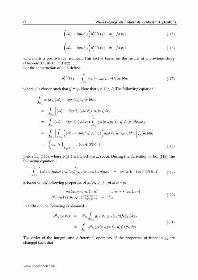
20

(115)

(116)

where p is a positive real number. This fact is based on the results of a previous study

(Theorem 3.1, Berthier, 1982).

For the construction of , define

(117)

where η is chosen such that η2 = ip. Note that η ∈ C \ B. The following equation:

(118)

yields Eq. (115), where (R+) is the Schwartz space. During the derivation of Eq. (118), the

following equation:

(119)

is based on the following properties of gij(x

3, y3, ξr, η) at x

3 = y3

(120)

In addition, the following is obtained:

(121)

The order of the integral and differential operators of the properties of function gij are

changed such that

www.intechopen.com


21

(122)

for an arbitrary positive integer n. According to Eq. (121), we have

(123)

It has been shown that uj ∈ L2(R+) from Lemma 2, so that ∈ D( ). The construction of

∈ D( ) is also possible. As a result, the following conclusion is obtained. □

4.3 Generalized Fourier transform for an elastic wave field in a half space The operator has been found to be self-adjoint and non-negative, which yields the following spectral representation:

(124)

where Eij is the spectral family. The spectral family is connected with the resolvent by

means of the Stone theorem (Wilcox, 1976):

(125)

for ui, vi ∈ L2(R+). Note that Rij is the resolvent of the operator and Rij(ζ)uj is defined by

(126)

Let and . Then, the right-hand side of Eq. (125) for the integral

becomes

(127)

where ζ = μ0η2 and ηR is defined by FR(ξr, ηR) = 0. The path of integration in the complex η plane shown in Fig. 5 is used for the evaluation of the integral.

In the following, the relationship between the right-hand side of Eq. (127) and the

eigenfunctions is presented. Let vi(x

3, ξr, η) ∈ D( ) satisfy

(128)

www.intechopen.com


22

Fig. 5. Path of the integral.

and define the scalar function W(η) such that

(129)

It is easy to derive the following properties of W(η) by means of the boundary conditions for

vi:

(130)

Note that vi(x

3, ξr, ηR) becomes the eigenfunction (Rayleigh wave mode) satisfying the free

boundary conditions. Otherwise, vi(x, ξr, η), (η ≠ ηR) cannot satisfy the free boundary

conditions. As a result, Eq. (130) is established. Integration by parts of Eq. (129) yields

(131)

where

(132)

The following lemma can then be obtained:

Lemma 3 The residue of gij at η = ηR can be expressed in terms of the eigenfunction such that

(133)

where ξ = (ξ1, ξ2, ηR) and ψim(x3, ξ) is the eigenfunction defined by

(134)

www.intechopen.com


23

[Proof]

Based on a previous study (Aki & Richards, 1980), the function gij can be constructed by

(135)

where wij is defined by

(136)

In addition, Δj is defined such that gij satisfies the free boundary condition:

(137)

The definition of W(η) shown in Eq. (129) implies that the expression is valid:

(138)

Equations (137) and (138) yield

(139)

Now, let η approach ηR. Due to reciprocity, it is found that

(140)

Therefore,

(141)

The residue of the resolvent kernel is expressed as

(142)

For the case in which the eigenfunction is normalized as I2(ηR) = 1, we have W ′(ηR) = −2μηR,

which concludes the proof. □

Next, the function gij:

(143)

is investigated for the case in which s = Re(η) > ξr. The function gij for this case is

constructed by

(144)

where vik is the definition function of the improper eigenfunction (Touhei, 2002). The

definition function vik satisfies the following:

www.intechopen.com


24

(145)

The relationship between the improper eigenfunction and the definition function is given as

(146)

Next, let us define the following function:

(147)

Substitution of the explicit forms of the eigenfunction and definition function of Eq. (147)

yields the following:

(148)

In addition, note that

(149)

which is obtained from the definition of wik shown in Eq. (136). Based on Eqs. (148) and

(149), the following lemma is obtained.

Lemma 4 For the region of s > ξr, the function gij satisfies the following equation:

(150)

where ψim(x

3, ξ) is the improper eigenfunction.

[Proof]

The requirement of the free boundary condition for gij yields the following expression of Δk┚:

(151)

Incorporating the following reciprocity relation:

(152)

into Eq. (151) yields

(153)

Therefore, the following is obtained:

(154)

Thus, Eqs. (146), (148), and (149) conclude the proof. □

www.intechopen.com


25

Next, let us again consider Eq. (127). Equation (127) holds for an arbitrary vi ∈ L2(R+), so that

the following equation can be obtained by incorporating the results of Lemmas 3 and 4:

(155)

where uj (ξr, · ) ∈ L2(R+), ξ = (ξ1, ξ2, ξ3) ∈ and

(156)

As mentioned earlier, and , so that

(157)

Therefore, Eqs. (125) and (155) yield

(158)

Let b in Eq. (158) approach infinity. Then, the following eigenfunction expansion form of ui

is obtained:

(159)

Note that the eigenfunction expansion form shown in Eq. (159) is that for ui(ξr, ·) having the

compact support. This result can be extended to all ui(ξr, · ) ∈ L2(R+) by a limiting

procedure, namely,

(160)

where the convergence is in L2(R+). The transform of the function in L2(R+) obtained here

can be summarized as follows:

www.intechopen.com


26

(161)

At this point, the transformation of the elastic wave field in a half space can be presented. Let us define the subset of the wavenumber space as follows:

(162)

The following theorem is obtained based on Eqs. (85), (95), and (158):

Theorem 2 There exists a map satisfying the free boundary condition of the elastic half space of the

wave field from L2( ) to L2(σp) ⊕ L2(σc) defined by

(163)

the inverse of which is

(164)

Here, and are expressed as follows:

(165)

where

(166)

Here, is referred to as the generalized Fourier transform of uj, and is referred

to as the generalized inverse Fourier transform of . Based on the literature (Reed and

Simon, 1975), the domain of the operators and could be extended from L2 to the

space of tempered distributions ′.

4.4 Method for the volume integral equation We have obtained the transform for elastic waves in a 3-D half space, which is to be applied to the volume integral equation. Preliminary to showing the application of the transform to

www.intechopen.com


27

the volume integral equation, we have to construct the Green’s function for the elastic half space based on the proposed transform. The definition of the Green’s function for the half space is expressed as

(167)

The application of the generalized Fourier transform to Eq. (167) yields

(168)

where is the generalized Fourier transform of the Green’s function. Therefore, as a result of Eq. (168), the Green’s function for a half space can be represented as

(169)

Next, let the function wi(x) be given in the following form:

(170)

The formal calculation reveals that

(171)

where denotes

(172)

Note that 1(· ) in Eq. (172) is defined such that

(173)

At this point, the application of the generalized Fourier transform to the volume integral equation becomes possible and is achieved as follows:

www.intechopen.com


28

(174)

where is the generalized Fourier transform of vi and is the incident wave field due to

the point source expressed by

(175)

The volume integral equation for the elastic wave equation in the wavenumber domain in a half space has the same structure as that in a full space. Therefore, almost the same numerical scheme based on the Krylov subspace iteration technique is available. Note that the difference in the numerical scheme between that for the elastic full space and that for the half space lies in the discretization of the wavenumber space. The discretization of the wavenumber space for elastic half space is as follows:

(176)

where Δξj , (j = 1, 2, 3) are the intervals of the grids in the wavenumber space,

(177)

and N1, N2, and N3 compose the set of integers defined by

(178)

where (N1,N2,N3) defines the number of grids in the wavenumber space. Note that Eq. (176)

corresponds to the decomposition of the Rayleigh and body waves.

4.5 Numerical example

For the numerical analysis of an elastic half space, the Lam´e constants of the background

structure is set such that λ0 = 4 GPa, μ0 = 2 GPa and the mass density is set at ρ =2 g/cm3.

Therefore, the background velocity of the P and S waves are 2 km/s and 1 km/s,

respectively. and that for the Rayleigh wave velocity is 0.93 km/s. In addition, the analyzed

frequency is f = 1 Hz.

First, let us investigate the accuracy of the generalized Fourier transform by composing the

Green’s function. For the calculation of the generalized Fourier transform, N1 = N2 = N3 = 256,

Δx

1 = Δx

2 = 0.25 km, and Δx

3=0.125 km are chosen to define Dx and Dξ. The parameter ε for

the Green’s function is set at 0.6. Figures 6(a) and 6(b) show the Green’s function calculated by the generalized Fourier transform and the Hankel transform. The distributions of the absolute displacements are shown is these figures. For the calculation of the Green’s function, the point source is set at a

www.intechopen.com


29

depth of 1 km from the free surface. The direction of the excitation force is vertical, and the

excitation force has an amplitude of 1.0 × 107 kN. Comparison of these figures reveals good agreement between the calculated results, which confirms the accuracy of the generalized Fourier transform.

(a) Generalized Fourier transform (b) Hankel transform

Fig. 6. Comparison of the Green’s function calculated by the generalized Fourier transform and the Hankel transform.

The following example shows the solution of the volume integral equation. The fluctuation of the elastic wave field is set as follows:

(179)

(180)

where A┣ and A┤ describe the amplitude of the fluctuation, ζ┣ and ζ┤ describe the spread of

the fluctuation in the space, and x

c is the center of the fluctuation. These parameters are set

at A┣ = A┤ = 0.6 GPa, ζ┣ = ζ┤ = 0.3 km−2 and

(181)

The fluctuation of the medium in the x

2 − x

3 plane at x

1 = 0 [km] is shown in Fig. 7.

Fig. 7. Fluctuation of the medium

In order to generate the scattered wave field, the location of the point source is set at x

s = (5,

0, 0) km. The direction of the excitation force is vertical, and the excitation force has an

www.intechopen.com


30

amplitude of 1×107 kN. Bi-CGSTAB method (Barrett et al., 1994) is used for the Krylov

subspace iteration technique. Figures 8 and 9 show the propagation of scattered waves at

the free surface and the amplitudes of the scattered waves in the x

1 − x

3 plane, respectively.

According to Fig. 8, the amplitudes of the scattered waves are larger in the forward region

of the fluctuating area, where x

1 < 0. Figure 9 shows that the propagation of the Rayleigh

waves as the scattered wvaes in the forwrad region. The amplitude of the scattered waves

are smaller in the fluctuating area. The scattered waves are found to be reflected at the

fluctuating area, thereby generating Rayleigh waves. The above numerical results explain

well the propagation of the scattered elastic waves in the half space.

Fig. 8. Scattering of waves at the free surface.

Fig. 9. Distribution of scattered waves in the vertical plane.

The numerical calculations were carried out using a computer with an AMD Opteron 2.4-GHz processor. The CPU time needed for iteration in Bi-CGSTAB was five hours, which is due primarily to the calculation of the generalized Fourier transforms. Note that the 2-D FFT for the horizontal coordinate system was used for the generalized Fourier transform. The transform for the vertical coordinate required a large CPU time. The reduction of this large CPU time requirement should be investigated in the future. The development of a fast algorithm for the generalized Fourier transforms may be required. It is also important to formulate the inverse scattering analysis method and to carry out the analysis.

5. Conclusions

In this chapter, a volume integral equation method was developed for elastic wave propagation for 3-D elastic full and half spaces. The developed method did not require the

www.intechopen.com


31

derivation of a coefficient matrix. Instead, the Fourier transform and the Krylov subspace iterative technique were used for the integral equation. The starting point of the formulation was the volume integral equation in the wavenumber domain. The Fourier transform and the inverse Fourier transform were repeatedly applied during the Krylov iterative process. Based on this procedure, a fast method was realized for both forward and inverse scattering analysis in a 3-D elastic full space via the fast Fourier transform and Bi-CGSTAB method. For example, if the number of iterations was two, the CPU time to obtain accurate solutions was only two minutes. Furthermore, for the inverse scattering problem, the reconstruction of inhomogeneities of the wave field was also successful, even for the multiple scattering problem. The ordinary Fourier transform is not valid for an elastic half space due to the boundary conditions at the free surface. The generalized Fourier transform and the inverse Fourier transform for elastic wave propagations in a half space were developed for the integral equation based on the spectral theory. The generalized Fourier transform composing the Green’s function was also verified numerically. The properties of the scattered wave field in a half space were found to be well explained by the proposed method. At present, the proposed method for an elastic half space requires a large amount of CPU time, which was five hours for the present numerical model. As such, a fast algorithm for the generalized Fourier transforms should be developed in the future.

6. References

Aki, K. and Richards, P.G. (1980). Quantitative Seismology, Theory and Methods., W. H. Freeman and Company.

Barrett, R., Berry, M., Chan, T.F., Demmel, J., Donato, J., Dongarra, J., Eijkhout, V., Pozo, R., Romine, C. and Van der Vorst, H. (1994). Templates for the solution of Linear Systems: Building Blocks for Iterative Methods, SIAM.

Bertheir, A.M. (1982). Spectral theory and wave operators for the Scrödinger equation, Research Notes in Mathematics, London, Pitman Advanced Publishing Program.

Colton, D. and Kress, R. (1983). Integral equation methods in scattering theory, New York, John Wiley and Sons, Inc.

Colton, D. and Kress, R. (1998). Inverse acoustic and electromagnetic scattering theory, Berlin, Heidelberg, Springer-Verlag.

De Zaeytijd, J., Bogaert, I. and Franchois, A. (2008). An efficient hybrid MLFMA-FFT solver for the volume integral equation in case of sparse 3D inhomogeneous dielectric scatterers, Journal of Computational Physics, 227, 7052-7068.

Fata, S.N. and Guzina, B.B. (2004). A linear sampling method for near-field inverse problems in elastodynamics, Inverse Problems, 20, 713-736.

Friedlander, F. G. and Joshi, M. (1998). Introduction to the theory of distributions, Cambridge University Press.

Guzina, B.B. and Chikichev, I. (2007). From imaging to material identification: A generalized concept of topological sensitivity, Journal of Mechanics and Physics of Solids, 55, 245-279.

Guzina, B. B., Fata, S.N. and Bonnet, M. (2003), On the stress-wave imaging of cavities in a semi-infinite solid, International Journal of Solids and Structures, 40, 1505-1523.

Hudson, J. A. and Heritage, J. R. (1981). The use of the Born approximation in seismic scattering problems, Geophys. J.R. Astr. Soc., 66, 221-240.

www.intechopen.com


32

Hörmander, L. (1983), The analysis of linear partial differential operators I, Springer-Verlag, Berlin, Heidelberg, 1983.

Ikebe, T. (1960). Eigenfunction expansion associated with the Schroedinger operators and their applications to scattering theory, Archive for Rational Mechanics and Analysis, 5, 1-34.

Kato, T. (1980). Perturbation Theory for Linear Operators, Berlin, Heidelberg, Springer-Verlag. Kleinman, R.E. and van den Berg, P.M. (1992). A modified gradient method for two-dimensional problems in tomography, Journal of Computational and Applied Mathematics, 42, 17-35.

Reed, M. and Simon, B. (1975). Method of Modern Mathematical Physics, Vol. II, Fourier Analysis and Self-adjointness, San Diego, Academic Press.

Touhei, T. (2002). Complete eigenfunction expansion form of the Green’s function for elastic layered half space, Archive of Applied mechanics, 72, 13-38.

Touhei, T. (2009). Generalized Fourier transform and its application to the volume integral equation for elastic wave propagation in a half space, International Journal of Solids and Structures, 46, 52-73.

Touhei,T., Kiuchi, T and Iwasaki (2009). A Fast Volume Integral Equation Method for the Direct/Inverse Problem in Elastic Wave Scattering Phenomena, International Journal of Solids and Structures, 46, 3860-3872.

Wilcox, C.H. (1976). Spectral analysis of the Pekeris operator, Arch. Rat. Mech. Anal., 60, pp. 259-300.

Yang, J., Abubaker, A., van den Berg, P.M., Habashy, T.M. and Reitich, F. (2008). A CG-FFT approach to the solution of a stress-velocity formulation of three-dimensional scattering problems, Journal of Computational physics, 227, 10018-10039.

www.intechopen.com

Wave Propagation in Materials for Modern ApplicationsEdited by Andrey Petrin

ISBN 978-953-7619-65-7Hard cover, 526 pagesPublisher InTechPublished online 01, January, 2010Published in print edition January, 2010

InTech Europe InTech China

In the recent decades, there has been a growing interest in micro- and nanotechnology. The advances innanotechnology give rise to new applications and new types of materials with unique electromagnetic andmechanical properties. This book is devoted to the modern methods in electrodynamics and acoustics, whichhave been developed to describe wave propagation in these modern materials and nanodevices. The bookconsists of original works of leading scientists in the field of wave propagation who produced new theoreticaland experimental methods in the research field and obtained new and important results. The first part of thebook consists of chapters with general mathematical methods and approaches to the problem of wavepropagation. A special attention is attracted to the advanced numerical methods fruitfully applied in the field ofwave propagation. The second part of the book is devoted to the problems of wave propagation in newlydeveloped metamaterials, micro- and nanostructures and porous media. In this part the interested reader willfind important and fundamental results on electromagnetic wave propagation in media with negative refractionindex and electromagnetic imaging in devices based on the materials. The third part of the book is devoted tothe problems of wave propagation in elastic and piezoelectric media. In the fourth part, the works on theproblems of wave propagation in plasma are collected. The fifth, sixth and seventh parts are devoted to theproblems of wave propagation in media with chemical reactions, in nonlinear and disperse media, respectively.And finally, in the eighth part of the book some experimental methods in wave propagations are considered. Itis necessary to emphasize that this book is not a textbook. It is important that the results combined in it aretaken “from the desks of researchers“. Therefore, I am sure that in this book the interested and activelyworking readers (scientists, engineers and students) will find many interesting results and new ideas.

How to referenceIn order to correctly reference this scholarly work, feel free to copy and paste the following:

Terumi Touhei (2010). A Volume Integral Equation Method for the Direct/Inverse Problem in Elastic WaveScattering Phenomena, Wave Propagation in Materials for Modern Applications, Andrey Petrin (Ed.), ISBN:978-953-7619-65-7, InTech, Available from: http://www.intechopen.com/books/wave-propagation-in-materials-for-modern-applications/a-volume-integral-equation-method-for-the-direct-inverse-problem-in-elastic-wave-scattering-phenomen

www.intechopen.com

University Campus STeP Ri Slavka Krautzeka 83/A 51000 Rijeka, Croatia Phone: +385 (51) 770 447 Fax: +385 (51) 686 166www.intechopen.com

Unit 405, Office Block, Hotel Equatorial Shanghai No.65, Yan An Road (West), Shanghai, 200040, China

Phone: +86-21-62489820 Fax: +86-21-62489821

© 2010 The Author(s). Licensee IntechOpen. This chapter is distributedunder the terms of the Creative Commons Attribution-NonCommercial-ShareAlike-3.0 License, which permits use, distribution and reproduction fornon-commercial purposes, provided the original is properly cited andderivative works building on this content are distributed under the samelicense.

https://creativecommons.org/licenses/by-nc-sa/3.0/

Documents

A Volume Integral Equation Method for the Direct/Inverse