A WELL-LOG REGRESSION ANALYSIS FOR P-WAVE VELOCITY ... · (S-wave) sonic log, while only a limited number of wells have the corresponding P-wave sonic logs. However, at well locations

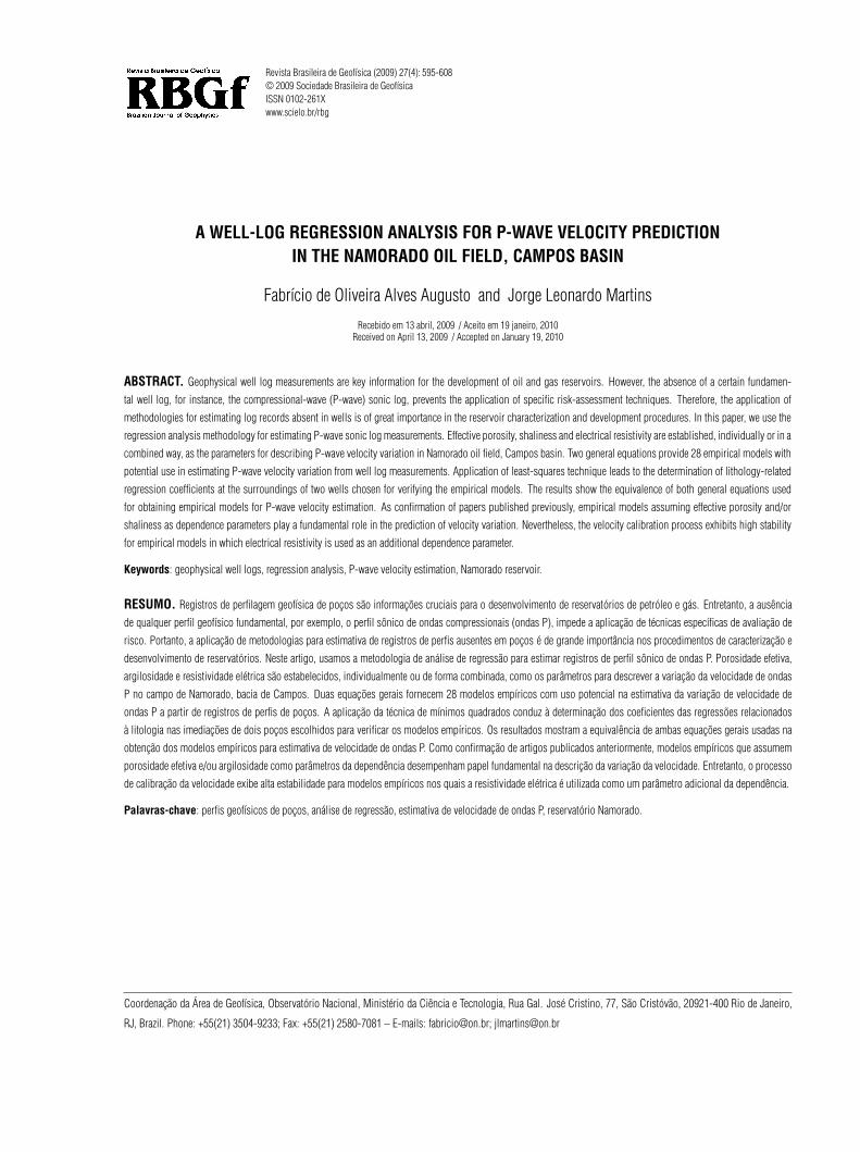
“main” — 2010/5/6 — 11:11 — page 595 — #1

Revista Brasileira de Geofısica (2009) 27(4): 595-608© 2009 Sociedade Brasileira de GeofısicaISSN 0102-261Xwww.scielo.br/rbg

A WELL-LOG REGRESSION ANALYSIS FOR P-WAVE VELOCITY PREDICTIONIN THE NAMORADO OIL FIELD, CAMPOS BASIN

Fabrıcio de Oliveira Alves Augusto and Jorge Leonardo Martins

Recebido em 13 abril, 2009 / Aceito em 19 janeiro, 2010Received on April 13, 2009 / Accepted on January 19, 2010

ABSTRACT. Geophysical well log measurements are key information for the development of oil and gas reservoirs. However, the absence of a certain fundamen-

tal well log, for instance, the compressional-wave (P-wave) sonic log, prevents the application of specific risk-assessment techniques. Therefore, the application of

methodologies for estimating log records absent in wells is of great importance in the reservoir characterization and development procedures. In this paper, we use the

regression analysis methodology for estimating P-wave sonic log measurements. Effective porosity, shaliness and electrical resistivity are established, individually or in a

combined way, as the parameters for describing P-wave velocity variation in Namorado oil field, Campos basin. Two general equations provide 28 empirical models with

potential use in estimating P-wave velocity variation from well log measurements. Application of least-squares technique leads to the determination of lithology-related

regression coefficients at the surroundings of two wells chosen for verifying the empirical models. The results show the equivalence of both general equations used

for obtaining empirical models for P-wave velocity estimation. As confirmation of papers published previously, empirical models assuming effective porosity and/or

shaliness as dependence parameters play a fundamental role in the prediction of velocity variation. Nevertheless, the velocity calibration process exhibits high stability

for empirical models in which electrical resistivity is used as an additional dependence parameter.

Keywords: geophysical well logs, regression analysis, P-wave velocity estimation, Namorado reservoir.

RESUMO. Registros de perfilagem geofısica de pocos sao informacoes cruciais para o desenvolvimento de reservatorios de petroleo e gas. Entretanto, a ausencia

de qualquer perfil geofısico fundamental, por exemplo, o perfil sonico de ondas compressionais (ondas P), impede a aplicacao de tecnicas especıficas de avaliacao de

risco. Portanto, a aplicacao de metodologias para estimativa de registros de perfis ausentes em pocos e de grande importancia nos procedimentos de caracterizacao e

desenvolvimento de reservatorios. Neste artigo, usamos a metodologia de analise de regressao para estimar registros de perfil sonico de ondas P. Porosidade efetiva,

argilosidade e resistividade eletrica sao estabelecidos, individualmente ou de forma combinada, como os parametros para descrever a variacao da velocidade de ondas

P no campo de Namorado, bacia de Campos. Duas equacoes gerais fornecem 28 modelos empıricos com uso potencial na estimativa da variacao de velocidade de

ondas P a partir de registros de perfis de pocos. A aplicacao da tecnica de mınimos quadrados conduz a determinacao dos coeficientes das regressoes relacionados

a litologia nas imediacoes de dois pocos escolhidos para verificar os modelos empıricos. Os resultados mostram a equivalencia de ambas equacoes gerais usadas na

obtencao dos modelos empıricos para estimativa de velocidade de ondas P. Como confirmacao de artigos publicados anteriormente, modelos empıricos que assumem

porosidade efetiva e/ou argilosidade como parametros da dependencia desempenham papel fundamental na descricao da variacao da velocidade. Entretanto, o processo

de calibracao da velocidade exibe alta estabilidade para modelos empıricos nos quais a resistividade eletrica e utilizada como um parametro adicional da dependencia.

Palavras-chave: perfis geofısicos de pocos, analise de regressao, estimativa de velocidade de ondas P, reservatorio Namorado.

Coordenacao da Area de Geofısica, Observatorio Nacional, Ministerio da Ciencia e Tecnologia, Rua Gal. Jose Cristino, 77, Sao Cristovao, 20921-400 Rio de Janeiro,

RJ, Brazil. Phone: +55(21) 3504-9233; Fax: +55(21) 2580-7081 – E-mails: [email protected]; [email protected]

“main” — 2010/5/6 — 11:11 — page 596 — #2

596 P-WAVE VELOCITY ESTIMATION USING WELL LOGS

INTRODUCTION

The geophysical development of an oil and gas field relies oncharacterizing the variation of petrophysical properties through-out the sedimentary interval containing the reservoirs (Archie,1950). In this way, laboratory measurements on core plugs, inter-pretation of geophysical well logs and inversion of seismic attri-butes provide valuable estimates of reservoir physical properties.Integration of these distinct methodologies is the best approachto determine uncertainties in the predictions, with direct implica-tions on risk mitigation in drilling operations (Pennington, 2001).

The estimation of any physical rock property implies to adopta mathematical model. However, the selected model hardly con-tains the full set of parameters affecting the rock property understudy. In general, the dependence of a given rock property is stu-died considering a parameter separately or combining relevantparameters in order to establish a corresponding mathematicalmodel. For instance, let us take the effective-medium theory mo-del routinely used in estimating total porosity from bulk densitylogs (Dewan, 1983; Ellis, 1987). The model establishes depen-dence of bulk density of a porous rock on mineralogy, porosityand fluid saturation. Nevertheless, depth and/or effective pres-sure are parameters ignored in the formulation of the effective-theory model for bulk density. The degree of rock consolidationtends to increase with depth due to effective pressure. As a re-sult of ignoring those parameters in the formulation, the estima-tive of total porosity using the bulk density model becomes sim-ple. However, no correlation of the density model with the rockconsolidation degree and effective pressure is allowed. A furtherexample is the estimation of rock elastic properties (i.e., seismicvelocities), which have parameter dependence yet more complex(Wyllie et al., 1956; Wyllie et al., 1958; Klimentos, 1991; Xu &White, 1995). In this case, the Voigt-Reuss and Hashin-Shtrikmaneffective medium theories (Watt et al., 1976) can be used for es-timating the elastic properties of mixed lithologies. However, cal-culations require detailed description on rock mineralogic cons-tituents and fluid content. Such a description demands timeand is often unavailable. Alternatively, use of Biot-Gassmannequations (Toksoz et al., 1976; Domenico, 1976) allows calcu-lating seismic velocities for dry or saturated porous rocks at low-and high-frequency ranges. However, the incompressibilities anddensities of the rock matrix and fluid, as well as the fractionaltotal porosity, must be a priori known for estimating seismicvelocities using Biot-Gassmann equations.

Assuming that a detailed description of the rock compositionis unavailable, regression analysis methodology is usually the

procedure used in the study of parameter dependence of seismicvelocities in mixed lithologies. In this instance, the investigationis highly simplified as long as individual or combined parameters(i.e., porosity, shaliness, fluid saturation, confining pressure, andothers) can be considered in the seismic velocity model formu-lation. Moreover, either ultrasonic measurements in core plugs(Tosaya & Nur, 1982; Han et al., 1986; Eberhart-Phillips et al.,1989) or well log data (Raymer et al., 1980; Castagna et al., 1985;Miller & Stewart, 1990) can be the source of information used inregression analysis for parameter dependence studies of seismicvelocities. In this way, interpreters gain insight for linking rockproperties to attributes investigated, for instance, in oil-bearingreservoir characterization procedures (Krief et al., 1990; Murphyet al., 1991; Castagna et al., 1993).

From Wyllie’s et al. (1956, 1958) time-average equation andRaymer et al. (1980) quadratic approach, rock porosity repre-sents the main parameter affecting P-wave velocities. However,both approximations can hardly predict velocity in shaly sands-tones without significant misfits. In order to consider additio-nal parameters into the velocity dependence, a useful strategy isthe application of multivariate linear regression methodologies.The papers of Tosaya & Nur (1982), Han et al. (1986) and Mil-ler & Stewart (1990) use rock porosity and shaliness to inves-tigate dependence of seismic velocities on both parameters indistinct mixed lithologies. As a result, including shaliness as afurther parameter into the dependence significantly increases cor-relation with velocity measurements. In turn, Eberhart-Phillips etal. (1989) used Han’s et al. (1986) core plug data to show thateffective pressure plays a significant role in predicting seismicvelocities. As a common conclusion from these cited works, po-rosity and shaliness play a fundamental role in the variation ofseismic velocities.

In this paper we refine the regression analysis methodologyused in previous investigations (see Han et al., 1986; Eberhart-Phillips et al., 1989; Miller & Stewart, 1990). We take into accountempirical models involving fractional effective porosity, shalinessand additionally electrical resistivity as dependence parametersof P-wave velocity variation. Incorporation of electrical resisti-vity into empirical models has the purpose of incorporating theeffects of fluid saturation on the velocity variation, as studied byDomenico (1974). Two general equations provide 28 multivari-ate linear and nonlinear empirical models, which served for es-timating P-wave velocity variation through the sedimentary inter-val corresponding to the upper Macae formation, Campos basin.Approximately 40 vertical wells were drilled through this turbidi-tic formation (Tigre & Lucchesi, 1986), through which anomalies

Revista Brasileira de Geofısica, Vol. 27(4), 2009

“main” — 2010/5/6 — 11:11 — page 597 — #3

FABRICIO DE OLIVEIRA ALVES AUGUSTO and JORGE LEONARDO MARTINS 597

in fundamental geophysical well log measurements reveal varia-tions of physical properties in the Namorado oil field. However,the absence of the P-wave sonic log in most wells prevents cons-tructing normal-incidence synthetic seismograms required forseismic calibration procedures. Hence, the establishment of P-wave velocity models allow sonic log estimation by using cor-respondent wells at the vicinities. Oliveira & Martins (2003) per-formed similar regression study using well log measurementsonly from the Namorado sandstone intervals. Here we extendedtheir regression methodology to the whole mixed lithology co-lumn representing the upper Macae formation. The well log re-gression methodology will be described in the next section.

METHODOLOGY

In the following, we present the steps for investigating the appli-cation of 28 empirical relations for predicting P-wave sonic logs.We selected two wells from the so-called data set “Campo Es-cola Namorado”, which is distributed by ANP/Brazil – AgenciaNacional do Petroleo, Gas Natural e Biocombustıveis, to Brazi-lian universities and research institutions for academic purpo-ses. The data set contains geological and geophysical well loginformation of more than 40 vertical wells drilled through theupper Macae formation. In this sedimentary interval the rockscorrespond mostly to sandstones and shales of turbiditic origin,forming the offshore oil-producing Namorado field in Camposbasin (Tigre & Lucchesi, 1986). Fundamental logs, i.e., gammaray (GR), deep electrical resistivity (ILD), neutron porosity (NPHI)and bulk density (RHOB) describe variation of physical propertiesthrough the formation at the surroundings of correspondent wells,allowing identification of the oil-bearing Namorado sandstone re-servoir. The well log data set has no information on shear-wave(S-wave) sonic log, while only a limited number of wells havethe corresponding P-wave sonic logs. However, at well locationswhere sonic logs are unavailable, linear and nonlinear empiricalmodels for the variation of P-wave velocity in the upper Macaeformation can be established. Based on information from the lite-rature, we assumed three main dependence parameters: the fracti-onal effective porosity φe, the fractional shale volume Vclay (i.e.,shaliness) and the deep electrical resistivity Rild. Conventionalprocessing of bulk density, gamma ray and induction resistivitylogs allows estimating the three mentioned dependence parame-ters. We applied the classical least-squares technique for deter-mining the regression coefficients of each empirical model. Usingthe correlation coefficient r, we measure the calibration step un-certainty. Below we summarize the steps of the methodology.

Selection of well logs

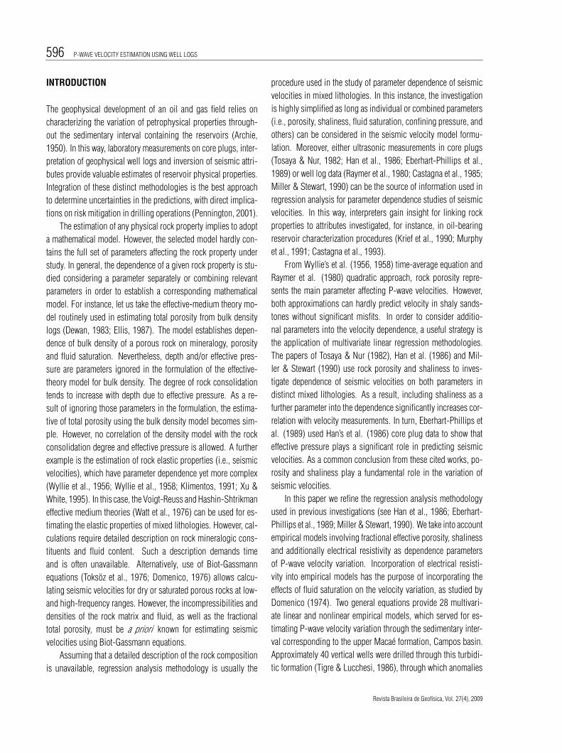
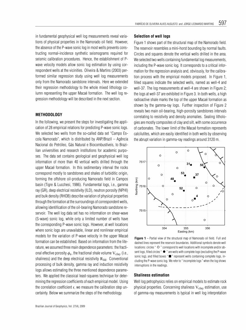
Figure 1 shows part of the structural map of the Namorado field.The reservoir resembles a mini-horst bounding by normal faults.Circles and squares denote the vertical wells drilled in the area.We selected two wells containing fundamental log measurements,including the P-wave sonic log. It corresponds to a critical infor-mation for the regression analysis and, obviously, for the calibra-tion process with the empirical models proposed. In Figure 1,filled squares indicate the selected wells, named as well-4 andwell-37. The log measurements at well-4 are shown in Figure 2;the logs at well-37 are exhibited in Figure 3. In both wells, a highradioactive shale marks the top of the upper Macae formation asshown by the gamma-ray logs. Further inspection of Figure 2reveals two main oil-bearing, high-porosity sandstones intervalscorrelating to resistivity and density anomalies. Sealing litholo-gies are mostly composites of clay and silt, with some occurrenceof carbonates. The lower limit of the Macae formation representscalcilutites, which are easily identified in both wells by observingthe abrupt variation in gamma-ray readings around 3120 m.

354 355 356

7515

7516

7517

Nor

thin

g (k

m)

Easting (km)

4

37

31 50

53

52

48

Figure 1 – Partial view of the structural map of Namorado oil field. Full anddashed lines represent the reservoir boundaries. Additional symbols denote welllocations: circles “ ◦ ” correspond to well locations with incomplete and/or ab-sent logs, filled circles “ • ” are wells with complete logs (excluding the P-wavesonic log), and filled boxes “� ” represent wells containing complete logs, in-cluding the P-wave sonic log. We refer to “ incomplete logs ” when the log showsinterruptions in the readings.

Shaliness estimation

Well log petrophysics relies on empirical models to estimate rockphysical properties. Concerning shaliness Vclay estimation, useof gamma-ray measurements is typical in well log interpretation

Brazilian Journal of Geophysics, Vol. 27(4), 2009

“main” — 2010/5/6 — 11:11 — page 598 — #4


100

101

102

103

104

2970

3010

3050

3090

3130

Dep

th (

m)

Rild

(Ohm.m)

(a)

0 50 100 150φ

N (%)

GR (API units)

(b)

2.5 3.5 4.5 5.5

ρb (g/cm3)

Vp (km/s)

(c)

0 20 40 60 80 100φ

e (%)

Vclay

(%)

(d)

Figure 2 – Geophysical logs at well-4: (a) induction resistivity (ILD, in blue) in Ohm.m; (b) neutron porosity (NPHI, in red) in percentage and gamma-rayGR (API units); (c) bulk density (RHOB, in red) in g/cm3 and the P-wave velocity vp (km/s) profile converted from the measured sonic log; (d) effectiveporosity (φe, in red) and shaliness Vclay, both in percentage. Application of Eqs. (1) and (3) allowed estimating Vclay and φe, respectively.

steps. In this case, Larionov (1969) presents empirical formu-las for Vclay estimation based on sediment consolidation. Takinginto account that the Namorado sandstone is from Tertiary age(i.e., the sediments are unconsolidated), we applied Larionov’s(1969) equation for shaliness estimation expressed as

Vclay = 0.083(

2 3.70 × IGR − 1)

. (1)

In the preceding equation, the gamma-ray index IGR is given by

IGR =GRi − GRss

GRsh − GRss, (2)

where GRi denotes the i th gamma-ray log reading. The quanti-ties GRss and GRsh are the minimum and maximum readingsin the gamma-ray log taken in the sandstone and in the shalepoint, respectively, in the same formation under study (Dewan,1983; Ellis, 1987). For the sedimentary interval correspon-ding to the upper Macae formation, GRss ≈ 22 API units andGRsh ≈ 125 API units.

Effective porosity estimation

The following formula allows fractional effective porosity φe esti-mation from the bulk density log:

φe = φt − Vclayρma − ρsh

ρma − ρf, (3)

where φt is the fractional total porosity

φt =ρma − ρb

ρma − ρf. (4)

The parameter ρb represents a reading in the bulk density log.As the upper Macae formation has quartzoze matrix, we takeρma = 2.65 g/cm3. For the brine formation density, we assumeρf = 1.10 g/cm3. Dewan (1983) shows that a way of assessingthe density at the shale point ρsh is to take the difference betweenthe neutron porosity log and the total porosity log at its maximum,i.e., max (φni − φti ), where φni and φti correspond to the i th

sample of the neutron porosity and the total porosity logs, res-pectively. In both wells under study the density at the shale pointis nearly ρsh = 2.66 g/cm3. Note that in Eq. (3) the shalinesscorrects the total porosity yielding the effective porosity φe.


“main” — 2010/5/6 — 11:11 — page 599 — #5


100

101

102

103

104

2970

3010

3050

3090

3130

Dep

th (

m)

Rild

(Ohm.m)

(a)

0 50 100 150φ

N (%)

GR (API units)

(b)

2.5 3.5 4.5 5.5

ρb (g/cm3)

Vp (km/s)

(c)

0 20 40 60 80 100φ

e (%)

Vclay

(%)

(d)

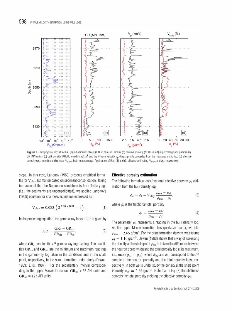
Figure 3 – Geophysical logs at well-37; logs are displayed using the same color code as in Figure 2. Eqs. (1) and (3) were also respectively consideredfor estimating the variation of shaliness and effective porosity.

Regression analysis

The dependence of P-wave velocity in rocks is attributed to nume-rous factors. However, in order to simplify the investigation, theevidence in most published papers is the use of empirical modelsattempting to correlate velocity variation with specific attributes.For example, correlation of velocities with depth and geologicaltime is presented in Faust (1951), while lithology is the parameterof the correlation in Faust (1953). Further empirical models fordescribing velocity variation based purely on mathematical func-tions can be found in Kaufman (1953).

In this paper, we assume the general dependence for P-wavevelocity model as vp = vp(x, y, z), in which the parametersof the dependence are: effective porosity x ≡ φe, shalinessy ≡ Vclay and electrical resistivity z ≡ Rild. The choice ofvp dependence was done taking the physical basis into account,and is corroborated by the results of several papers (see Han et al.,1986; Miller & Stewart, 1990; Oliveira & Martins, 2003). Thus,assuming x ≡ φe and y ≡ Vclay, we followed the work of pre-vious investigators. Moreover, the incorporation of z ≡ Rild intosome empirical models led to the known dependence of P-wavevelocity on fluid saturation.

The following general relations allow the investigation of li-near and nonlinear empirical models for P-wave velocity predic-tion from well log measurements:

vpmod = VP0 +VP1 +VP2 +VP3 (5)

and

vpmod = VP0 exp

[VP1 +VP2 +VP3

]. (6)

The above quantities VP0,VP1 ≡ VP1(x, y, z),VP2 ≡VP2(x, y, z) andVP3 ≡ VP3(x, y, z) are written as

VP0 ≡ a0, (7)

VP1 ≡ a1 x + a2 y + a3 z, (8)

VP2 ≡ a4 x y + a5 x z + a6 y z, (9)

and

VP3 ≡ a7 x2 + a8 y2 + a9 z2. (10)

We tested the whole set of combinations for empirical formulaspossibly provided by Eqs. (5) and (6). These models are easily


“main” — 2010/5/6 — 11:11 — page 600 — #6


obtained by assuming a dependence of vp on a single parameter,or taking more than one parameter simultaneously in the depen-dence. For instance, assuming a simple model in which the fracti-onal effective porosity φe is the only parameter of the dependence,we can write a linear model for P-wave velocity variation

vpmod = a0 + a1 φe. (11)

In accordance to Eq. (6), a nonlinear dependence on φe can alsobe provided for vp, as follows

vpmod = a0 exp

[a1 φe

]. (12)

As in Castagna et al. (1993), we can also use the simple pa-rabolic model with y ≡ Vclay as the only parameter affecting vp.As a result, we obtain from Eq. (5)

vpmod = a0 + a2 Vclay + a8

(Vclay

)2, (13)

On the other hand, Eq. (6) gives a nonlinear empirical model forvp as a function of Vclay:

vpmod = a0 exp

[a2 Vclay + a8

(Vclay

)2 ]. (14)

Besides multivariate linear models as in Han et al. (1986) andin Eberhart-Phillips et al. (1989), Eqs. (5) and (6) also allow toderive nonlinear models. For instance, assuming the parameterdependence vp ≡ vp(φe, Vclay, Rild), P-wave velocity can bedescribed by the following multivariate linear model

vpmod = a0 + a1 φe + a2 Vclay + a3 Rild, (15)

or, from the general form in Eq. (6), by a multivariate nonlinearmodel written as

vpmod = a0 exp

[a1 φe + a2 Vclay + a3 Rild

]. (16)

Two- and three-variable quadratic empirical models can alsobe derived from Eqs. (5) and (6). Taking x ≡ φe and z ≡ Rild asthe parameters of the dependence, the P-wave velocity variationcan be described as

vpmod = a0 + a1 φe + a3 Rild + a5 φe Rild

+ a7 (φe)2 + a9 (Rild)

2,

(17)

and

vpmod = a0 exp

[a1 φe + a3 Rild + a5 φe Rild

+ a7 (φe)2 + a9 (Rild)

2 ].

(18)

In summary, we investigated 28 empirical models for predictingP-wave velocities using geophysical well logs. In order to deter-mine the regression coefficients ai of the corresponding empiricalmodel, we applied the classical least-squares technique (Lines& Treitel, 1984). We thus minimized the square of the residu-als between the measured velocity vmeas

p (i.e., the readings in theP-wave sonic log) and the modeled velocity vmod

p (i.e., the cho-sen empirical model). As a result, after constructing the objectivefunction E2 ≡ E2(ai )

E2 = | vpmeas − vp

mod |2 (19)

we operate ∂E2/∂ai ≡ 0. The sought coefficients ai are theunknowns of the resulting linear system of equations derived af-ter minimizing Eq. (19). Notice that we applied the neperian lo-garithm to both sides of Eq. (6) before operating the derivativeof the objective function. Furthermore, we determined the cor-relation coefficient r in order to investigate the uncertainty in thepredictions of P-wave velocities.

Calibration

In the calibration step, we focused on plotting the P-wave velocitylogs at both selected wells and the empirical models provided byEqs. (5) and (6). This procedure aimed at visually inspecting themisfits between measured and predicted vp velocity logs. Furtherdetermination of correlation coefficients of the least-squares re-gression models and absolute residuals helped analyzing the con-fidence on the investigated empirical models.

RESULTS

Following the methodology described above, we combined thedependence parameters φe, Vclay and Rild in order to obtain mo-dels for vp velocity variation at both selected wells (see Fig. 1).The least-squares regression coefficients for all 28 empirical mo-dels derived from Eqs. (5) and (6) are exhibited in Tables 1-4. Observing the magnitude of the correlation coefficient forcorresponding empirical models, we immediately conclude thatthe general forms in Eqs. (5) and (6) provide equivalent P-wavevelocity predictions.

For empirical models with only one variable, it can be obser-ved in the tables that the correlation coefficient reaches the highestmagnitude if the effective porosity φe is chosen for describing vp

dependence. On the other hand, if the parameter of the depen-dence is the resistivity Rild, the correlation coefficient attains thesmallest magnitude. This is indeed an expected result already pu-blished in Han et al. (1986), that is, porosity plays a fundamental


“main” — 2010/5/6 — 11:11 — page 601 — #7


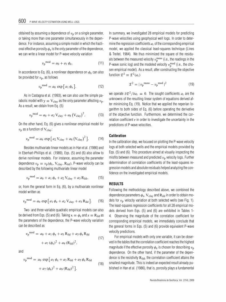
Table 1 – Least-squares regression coefficients for P-wave velocity models at well-4. Two general forms are considered: vp =a0 +a1 x +a2 y +a3 z and vp = a0 exp[ a1 x+a2 y +a3 z ]. Fractional effective porosity (x ≡ φe), shaliness (y ≡ Vclay)and electrical resistivity (z ≡ Rild in Ohm.m) are the parameters of the dependence shown in the first column of the table. Eachcolumn in (a) and (b) provides six empirical models. Between braces are the coefficients associated to exponential empirical models.In order to obtain a velocity model, simply neglect one or two dependence parameters in both considered general forms. The lastcolumn in (c) provides the two empirical models having full parameter dependence. Regression coefficients have units in such a waythat vp is in km/s. The symbol r stands for correlation coefficient.

PD (a) (b) (c)

x φe φe φe φe

y Vclay Vclay Vclay Vclayz Rild Rild Rild Rild

a0 4.27 3.92 3.72 3.97 4.29 4.42 4.43a1 -4.00 -4.40 -3.76 -4.06a2 -1.79 -1.84 -1.44 -1.38a3 -3.56×10−3 -4.05×10−3 3.30×10−3 2.40×10−3

r 0.70 0.42 0.17 0.47 0.72 0.78 0.79

{a0} 4.26 3.87 3.69 3.93 4.28 4.43 4.44{a1} -1.06 -1.15 -9.90×10−1 -1.07{a2} -4.60×10−1 -4.70×10−1 -3.60×10−1 -3.50×10−1

{a3} -9.88×10−4 -1.11×10−3 8.16×10−4 5.87×10−4

{r} 0.71 0.45 0.17 0.49 0.73 0.79 0.80

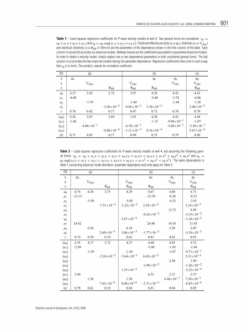
Table 2 – Least-squares regression coefficients for P-wave velocity models at well-4, but assuming the following gene-ral forms: vp = a0 + a1 x + a2 y + a3 z + a4 x y + a5 x z + a6 y z + a7 x2 + a8 y2 + a9 z2 and vp =a0 exp[ a1 x + a2 y + a3 z + a4 x y + a5 x z + a6 y z + a7 x2 + a8 y2 + a9 z2 ]. The same observations inTable 1 concerning empirical model derivation, parameter dependence and units apply for Table 2.

PD (a) (b) (c)

x φe φe φe φe

y Vclay Vclay Vclay Vclayz Rild Rild Rild Rild

a0 4.74 4.20 3.75 4.29 4.67 4.80 4.71a1 -12.15 -12.59 -8.20 -8.23a2 -5.50 -5.65 -4.32 -3.91a3 -7.51×10−3 -1.22×10−2 2.59×10−2 2.14×10−2

a4 12.72 8.99a5 -8.24×10−2 -5.35×10−2

a6 3.87×10−2 -1.18×10−3

a7 24.82 26.90 10.43 11.45a8 6.26 6.18 2.58 2.85a9 2.69×10−5 3.06×10−5 -1.77×10−5 -3.18×10−5

r 0.74 0.59 0.19 0.62 0.81 0.83 0.85

{a0} 4.76 4.17 3.72 4.27 4.68 4.83 4.72{a1} -2.99 -3.09 -1.95 -1.94{a2} -1.39 -1.45 -1.07 -9.71×10−1

{a3} -2.10×10−3 -3.64×10−3 6.45×10−3 5.31×10−3

{a4} 2.94 1.99{a5} -1.99×10−2 -1.26×10−2

{a6} 1.25×10−2 -2.32×10−4

{a7} 5.89 6.35 2.21 2.37{a8} 1.58 1.56 6.48×10−1 7.28×10−1

{a9} 7.63×10−6 8.90×10−6 -3.71×10−6 -8.85×10−6

{r} 0.78 0.61 0.19 0.64 0.81 0.84 0.85


“main” — 2010/5/6 — 11:11 — page 602 — #8


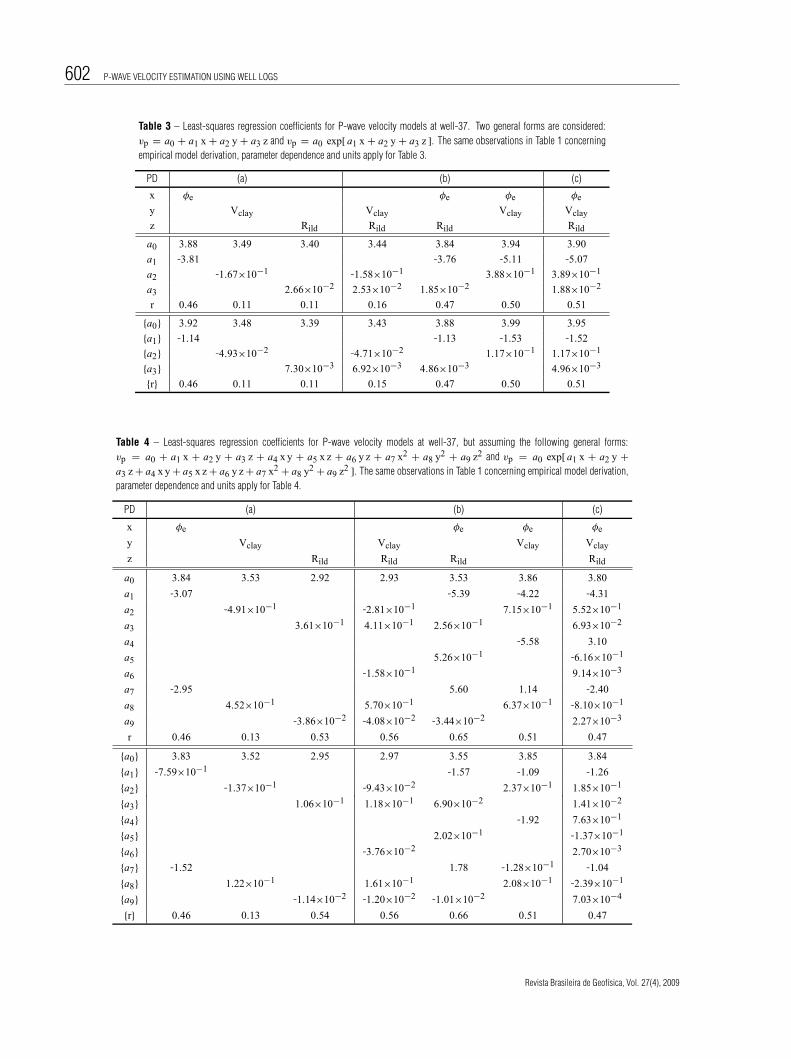
Table 3 – Least-squares regression coefficients for P-wave velocity models at well-37. Two general forms are considered:vp = a0 + a1 x + a2 y + a3 z and vp = a0 exp[ a1 x + a2 y + a3 z ]. The same observations in Table 1 concerningempirical model derivation, parameter dependence and units apply for Table 3.

PD (a) (b) (c)

x φe φe φe φe

y Vclay Vclay Vclay Vclay

z Rild Rild Rild Rild

a0 3.88 3.49 3.40 3.44 3.84 3.94 3.90

a1 -3.81 -3.76 -5.11 -5.07

a2 -1.67×10−1 -1.58×10−1 3.88×10−1 3.89×10−1

a3 2.66×10−2 2.53×10−2 1.85×10−2 1.88×10−2

r 0.46 0.11 0.11 0.16 0.47 0.50 0.51

{a0} 3.92 3.48 3.39 3.43 3.88 3.99 3.95

{a1} -1.14 -1.13 -1.53 -1.52

{a2} -4.93×10−2 -4.71×10−2 1.17×10−1 1.17×10−1

{a3} 7.30×10−3 6.92×10−3 4.86×10−3 4.96×10−3

{r} 0.46 0.11 0.11 0.15 0.47 0.50 0.51

Table 4 – Least-squares regression coefficients for P-wave velocity models at well-37, but assuming the following general forms:vp = a0 + a1 x + a2 y + a3 z + a4 x y + a5 x z + a6 y z + a7 x2 + a8 y2 + a9 z2 and vp = a0 exp[ a1 x + a2 y +a3 z + a4 x y + a5 x z + a6 y z + a7 x2 + a8 y2 + a9 z2 ]. The same observations in Table 1 concerning empirical model derivation,parameter dependence and units apply for Table 4.

PD (a) (b) (c)

x φe φe φe φe

y Vclay Vclay Vclay Vclay

z Rild Rild Rild Rild

a0 3.84 3.53 2.92 2.93 3.53 3.86 3.80

a1 -3.07 -5.39 -4.22 -4.31

a2 -4.91×10−1 -2.81×10−1 7.15×10−1 5.52×10−1

a3 3.61×10−1 4.11×10−1 2.56×10−1 6.93×10−2

a4 -5.58 3.10

a5 5.26×10−1 -6.16×10−1

a6 -1.58×10−1 9.14×10−3

a7 -2.95 5.60 1.14 -2.40

a8 4.52×10−1 5.70×10−1 6.37×10−1 -8.10×10−1

a9 -3.86×10−2 -4.08×10−2 -3.44×10−2 2.27×10−3

r 0.46 0.13 0.53 0.56 0.65 0.51 0.47

{a0} 3.83 3.52 2.95 2.97 3.55 3.85 3.84

{a1} -7.59×10−1 -1.57 -1.09 -1.26

{a2} -1.37×10−1 -9.43×10−2 2.37×10−1 1.85×10−1

{a3} 1.06×10−1 1.18×10−1 6.90×10−2 1.41×10−2

{a4} -1.92 7.63×10−1

{a5} 2.02×10−1 -1.37×10−1

{a6} -3.76×10−2 2.70×10−3

{a7} -1.52 1.78 -1.28×10−1 -1.04

{a8} 1.22×10−1 1.61×10−1 2.08×10−1 -2.39×10−1

{a9} -1.14×10−2 -1.20×10−2 -1.01×10−2 7.03×10−4

{r} 0.46 0.13 0.54 0.56 0.66 0.51 0.47


“main” — 2010/5/6 — 11:11 — page 603 — #9


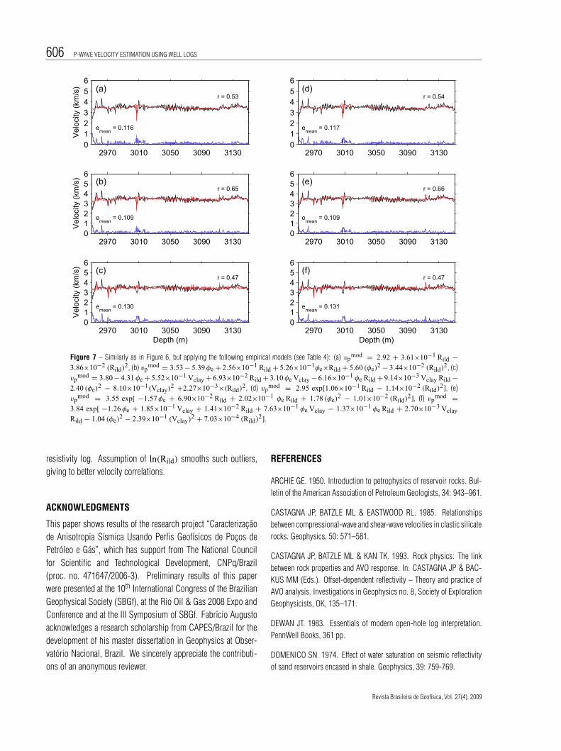
role in the variation of P-wave velocity, while the influence of sha-liness Vclay is smaller than φe. The assumption of resistivity as aparameter of influence in the vp variation represents an attempt ofconsidering fluid saturation. However, the resistivity Rild exertsthe smallest influence on vp variation. Note that the results inthe third column of Table 4a represent an exception. We interpretthese results as the footprint of the well-behaved resistivity andporosity logs at well-37. At this well, it seems that fluid contentpredominantly influences the velocities. A further interesting re-sult can be obtained as follows. Let us consider all 2-variable em-pirical models in which φe and Vclay are the governing parame-ters in the vp variation. If we assume φe and Vclay as null quan-tities in these velocity models, the maximum P-wave velocity forthe considered quartzoze matrix will hardly be vp = 4.90 km/sas seen in the third column of item (b) of all tables. Taking intoaccount that vp = 5.94 km/s is the velocity value recommendedfor quartz (Wyllie et al., 1958), the latter result for Vclay = 0.0

clearly indicates the influence of other different lithologies (i.e.,carbonates) present in the formation. Actually, this analysis canbe applied for all empirical models used in this investigation. Thevelocity calibration using the above-mentioned empirical modelsis presented in the Figures 4 and 6, including the correspondingequivalent models obtained from Eq. (6).

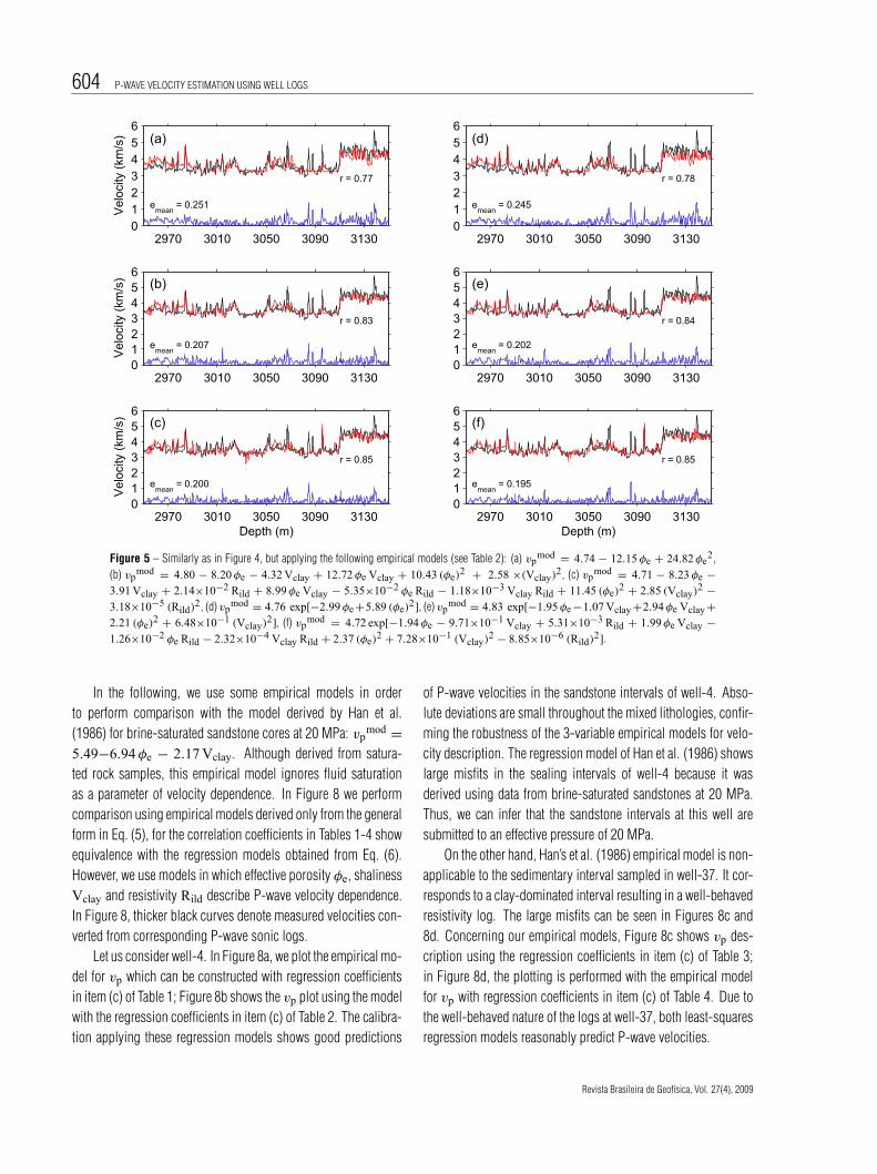
In Tables 2a and 4a, the magnitude of the correlation coeffici-ents shows that use of quadratic regression models improves theconfidence on P-wave velocity predictions. The plots in Figures5 and 7 exhibits velocity calibration for both wells under investi-gation, confirming the high performance of all quadratic modelsused. In summary, incorporation of quadratic terms into the empi-rical models decreases the misfits between measured and predic-ted velocities. As pointed out above, the small-magnitude discre-pancies between measured and predicted velocities reveal furtherinfluence of other mixed lithologies forming the sedimentary in-terval under analysis.

2970 3010 3050 3090 31300123456

(a)

emean

= 0.288

r = 0.70

Vel

ocity

(km

/s)

2970 3010 3050 3090 31300123456

(b)

emean

= 0.246

r = 0.78

Vel

ocity

(km

/s)

2970 3010 3050 3090 31300123456

(c)

emean

= 0.243

r = 0.79

Depth (m)

Vel

ocity

(km

/s)

2970 3010 3050 3090 31300123456

(d)

emean

= 0.279

r = 0.71

2970 3010 3050 3090 31300123456

(e)

emean

= 0.238

r = 0.79

2970 3010 3050 3090 31300123456

(f)

emean

= 0.235

r = 0.80

Depth (m)

Figure 4 – Application of regression models for P-wave velocity prediction vpmod at well-4. Black curve denotes P-wave velocity vp

meas

converted from measured sonic log. In accordance with the regression coefficients in Table 1, the empirical models (red curves) are: (a)vp

mod = 4.27−4.00 φe, (b) vpmod = 4.42−3.76 φe −1.44 Vclay, (c) vp

mod = 4.43−4.06 φe −1.38 Vclay + 2.40× 10−3 Rild, (d)vp

mod = 4.26× exp[−1.06 φe], (e) vpmod = 4.43 exp[−0.99 φe − 0.36 Vclay], (f) vp

mod = 4.44 exp[−1.07 φe − 0.35 Vclay +5.87×10−4 Rild]. Blue curves represent absolute residuals between measured and predicted velocity logs. Each plot correspondingly shows themean absolute residual emean and the correlation coefficient r.


“main” — 2010/5/6 — 11:11 — page 604 — #10


2970 3010 3050 3090 31300123456

(a)

emean

= 0.251

r = 0.77

Vel

ocity

(km

/s)

2970 3010 3050 3090 31300123456

(b)

emean

= 0.207

r = 0.83

Vel

ocity

(km

/s)

2970 3010 3050 3090 31300123456

(c)

emean

= 0.200

r = 0.85

Depth (m)

Vel

ocity

(km

/s)

2970 3010 3050 3090 31300123456

(d)

emean

= 0.245

r = 0.78

2970 3010 3050 3090 31300123456

(e)

emean

= 0.202

r = 0.84

2970 3010 3050 3090 31300123456

(f)

emean

= 0.195

r = 0.85

Depth (m)

Figure 5 – Similarly as in Figure 4, but applying the following empirical models (see Table 2): (a) vpmod = 4.74 − 12.15 φe + 24.82 φe

2,(b) vp

mod = 4.80 − 8.20 φe − 4.32 Vclay + 12.72 φe Vclay + 10.43 (φe)2 + 2.58 ×(Vclay)2, (c) vp

mod = 4.71 − 8.23 φe −3.91 Vclay + 2.14×10−2 Rild + 8.99 φe Vclay − 5.35×10−2 φe Rild − 1.18×10−3 Vclay Rild + 11.45 (φe)

2 + 2.85 (Vclay)2 −3.18×10−5 (Rild)2, (d) vp

mod = 4.76 exp[−2.99 φe +5.89 (φe)2], (e) vp

mod = 4.83 exp[−1.95 φe −1.07 Vclay +2.94 φe Vclay +2.21 (φe)

2 + 6.48×10−1 (Vclay)2], (f) vpmod = 4.72 exp[−1.94 φe − 9.71×10−1 Vclay + 5.31×10−3 Rild + 1.99 φe Vclay −

1.26×10−2 φe Rild − 2.32×10−4 Vclay Rild + 2.37 (φe)2 + 7.28×10−1 (Vclay)2 − 8.85×10−6 (Rild)2].

In the following, we use some empirical models in orderto perform comparison with the model derived by Han et al.(1986) for brine-saturated sandstone cores at 20 MPa: vp

mod =5.49−6.94 φe − 2.17 Vclay. Although derived from satura-ted rock samples, this empirical model ignores fluid saturationas a parameter of velocity dependence. In Figure 8 we performcomparison using empirical models derived only from the generalform in Eq. (5), for the correlation coefficients in Tables 1-4 showequivalence with the regression models obtained from Eq. (6).However, we use models in which effective porosity φe, shalinessVclay and resistivity Rild describe P-wave velocity dependence.In Figure 8, thicker black curves denote measured velocities con-verted from corresponding P-wave sonic logs.

Let us consider well-4. In Figure 8a, we plot the empirical mo-del for vp which can be constructed with regression coefficientsin item (c) of Table 1; Figure 8b shows the vp plot using the modelwith the regression coefficients in item (c) of Table 2. The calibra-tion applying these regression models shows good predictions

of P-wave velocities in the sandstone intervals of well-4. Abso-lute deviations are small throughout the mixed lithologies, confir-ming the robustness of the 3-variable empirical models for velo-city description. The regression model of Han et al. (1986) showslarge misfits in the sealing intervals of well-4 because it wasderived using data from brine-saturated sandstones at 20 MPa.Thus, we can infer that the sandstone intervals at this well aresubmitted to an effective pressure of 20 MPa.

On the other hand, Han’s et al. (1986) empirical model is non-applicable to the sedimentary interval sampled in well-37. It cor-responds to a clay-dominated interval resulting in a well-behavedresistivity log. The large misfits can be seen in Figures 8c and8d. Concerning our empirical models, Figure 8c shows vp des-cription using the regression coefficients in item (c) of Table 3;in Figure 8d, the plotting is performed with the empirical modelfor vp with regression coefficients in item (c) of Table 4. Due tothe well-behaved nature of the logs at well-37, both least-squaresregression models reasonably predict P-wave velocities.


“main” — 2010/5/6 — 11:11 — page 605 — #11


2970 3010 3050 3090 31300123456

emean

= 0.135

r = 0.46(a)

Vel

ocity

(km

/s)

2970 3010 3050 3090 31300123456

emean

= 0.129

r = 0.50(b)

Vel

ocity

(km

/s)

2970 3010 3050 3090 31300123456

emean

= 0.127

r = 0.51(c)

Depth (m)

Vel

ocity

(km

/s)

2970 3010 3050 3090 31300123456

emean

= 0.136

r = 0.46(d)

2970 3010 3050 3090 31300123456

emean

= 0.130

r = 0.50(e)

2970 3010 3050 3090 31300123456

emean

= 0.128

r = 0.51(f)

Depth (m)

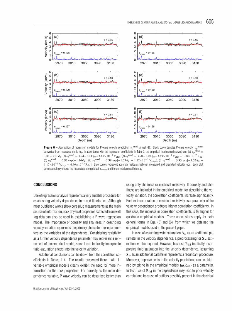
Figure 6 – Application of regression models for P-wave velocity prediction vpmod at well-37. Black curve denotes P-wave velocity vp

meas

converted from measured sonic log. In accordance with the regression coefficients in Table 3, the empirical models (red curves) are: (a) vpmod =

3.88−3.81 φe, (b) vpmod = 3.94−5.11 φe+3.88×10−1 Vclay, (c) vp

mod = 3.90−5.07 φe+3.89×10−1 Vclay+1.88×10−2 Rild,(d) vp

mod = 3.92 exp[−1.14 φe], (e) vpmod = 3.99 exp[−1.53 φe + 1.17×10−1 Vclay], (f) vp

mod = 3.95 exp[−1.52 φe +1.17×10−1 Vclay + 4.96×10−3 Rild]. Blue curves represent absolute residuals between measured and predicted velocity logs. Each plotcorrespondingly shows the mean absolute residual emean and the correlation coefficient r.

CONCLUSIONS

Use of regression analysis represents a very suitable procedure forestablishing velocity dependence in mixed lithologies. Althoughmost published works show core plug measurements as the mainsource of information, rock physical properties extracted from welllog data can also be used in establishing a P-wave regressionmodel. The importance of porosity and shaliness in describingvelocity variation represents the primary choice for these parame-ters as the variables of the dependence. Considering resistivityas a further velocity dependence parameter may represent a refi-nement of the empirical model, since it can indirectly incorporatefluid-saturation effects into the velocity variation.

Additional conclusions can be drawn from the correlation co-efficients in Tables 1-4. The results presented therein with 1-variable empirical models clearly exhibit the need for more in-formation on the rock properties. For porosity as the main de-pendence variable, P-wave velocity can be described better than

using only shaliness or electrical resistivity. If porosity and sha-liness are included in the empirical model for describing the ve-locity variation, the correlation coefficients increase significantly.Further incorporation of electrical resistivity as a parameter of thevelocity dependence produces higher correlation coefficients. Inthis case, the increase in correlation coefficients is far higher forquadratic empirical models. These conclusions apply for bothgeneral forms in Eqs. (5) and (6), from which we obtained theempirical models used in the present paper.

In case of assuming water saturation Sw as an additional pa-rameter in the velocity dependence, a preprocessing for Sw esti-mation will be required. However, because Rild implicitly incor-porates fluid saturation into the velocity dependence, assumingSw as an additional parameter represents a redundant procedure.Moreover, improvements in the velocity predictions can be obtai-ned by taking in the empirical models ln(Rild) as a parameter.In fact, use of Rild in the dependence may lead to poor velocitycorrelations because of outliers possibly present in the electrical


“main” — 2010/5/6 — 11:11 — page 606 — #12


2970 3010 3050 3090 31300123456

emean

= 0.116

r = 0.53(a)

Vel

ocity

(km

/s)

2970 3010 3050 3090 31300123456

emean

= 0.109

r = 0.65(b)

Vel

ocity

(km

/s)

2970 3010 3050 3090 31300123456

emean

= 0.130

r = 0.47(c)

Depth (m)

Vel

ocity

(km

/s)

2970 3010 3050 3090 31300123456

emean

= 0.117

r = 0.54(d)

2970 3010 3050 3090 31300123456

emean

= 0.109

r = 0.66(e)

2970 3010 3050 3090 31300123456

emean

= 0.131

r = 0.47(f)

Depth (m)

Figure 7 – Similarly as in Figure 6, but applying the following empirical models (see Table 4): (a) vpmod = 2.92 + 3.61×10−1 Rild −

3.86×10−2 (Rild)2, (b) vpmod = 3.53 − 5.39 φe + 2.56×10−1 Rild + 5.26×10−1φe×Rild + 5.60 (φe)

2 − 3.44×10−2 (Rild)2, (c)vp

mod = 3.80 − 4.31 φe + 5.52×10−1 Vclay + 6.93×10−2 Rild + 3.10 φe Vclay − 6.16×10−1 φe Rild + 9.14×10−3 Vclay Rild −2.40 (φe)

2 − 8.10×10−1(Vclay)2 +2.27×10−3×(Rild)2, (d) vpmod = 2.95 exp[1.06×10−1 Rild − 1.14×10−2 (Rild)2], (e)

vpmod = 3.55 exp[ −1.57 φe + 6.90×10−2 Rild + 2.02×10−1 φe Rild + 1.78 (φe)

2 − 1.01×10−2 (Rild)2], (f) vpmod =

3.84 exp[ −1.26 φe + 1.85×10−1 Vclay + 1.41×10−2 Rild + 7.63×10−1 φe Vclay − 1.37×10−1 φe Rild + 2.70×10−3 VclayRild − 1.04 (φe)

2 − 2.39×10−1 (Vclay)2 + 7.03×10−4 (Rild)2].

resistivity log. Assumption of ln(Rild) smooths such outliers,giving to better velocity correlations.

ACKNOWLEDGMENTS

This paper shows results of the research project “Caracterizacaode Anisotropia Sısmica Usando Perfis Geofısicos de Pocos dePetroleo e Gas”, which has support from The National Councilfor Scientific and Technological Development, CNPq/Brazil(proc. no. 471647/2006-3). Preliminary results of this paperwere presented at the 10th International Congress of the BrazilianGeophysical Society (SBGf), at the Rio Oil & Gas 2008 Expo andConference and at the III Symposium of SBGf. Fabrıcio Augustoacknowledges a research scholarship from CAPES/Brazil for thedevelopment of his master dissertation in Geophysics at Obser-vatorio Nacional, Brazil. We sincerely appreciate the contributi-ons of an anonymous reviewer.

REFERENCES

ARCHIE GE. 1950. Introduction to petrophysics of reservoir rocks. Bul-

letin of the American Association of Petroleum Geologists, 34: 943–961.

CASTAGNA JP, BATZLE ML & EASTWOOD RL. 1985. Relationships

between compressional-wave and shear-wave velocities in clastic silicate

rocks. Geophysics, 50: 571–581.

CASTAGNA JP, BATZLE ML & KAN TK. 1993. Rock physics: The link

between rock properties and AVO response. In: CASTAGNA JP & BAC-

KUS MM (Eds.). Offset-dependent reflectivity – Theory and practice of

AVO analysis. Investigations in Geophysics no. 8, Society of Exploration

Geophysicists, OK, 135–171.

DEWAN JT. 1983. Essentials of modern open-hole log interpretation.

PennWell Books, 361 pp.

DOMENICO SN. 1974. Effect of water saturation on seismic reflectivity

of sand reservoirs encased in shale. Geophysics, 39: 759-769.


“main” — 2010/5/6 — 11:11 — page 607 — #13


0 1 2 3 4 5 6

2970

3010

3050

3090

3130

(a)

Dep

th (

m)

0 1 2 3 4 5 6(b)

0 1 2 3 4 5 6(c)

0 1 2 3 4 5 6(d)

Figure 8 – Comparison of regression models for P-wave velocity prediction. The comparison is performed using the empirical relation inHan et al. (1986) for rock plugs submitted to an effective pressure of 20 MPa: vp

mod = 5.49 − 6.94 φe − 2.17 Vclay (blue curve).At well-4 (red curves): (a) vp

mod = 4.43 − 4.06 φe − 1.38 Vclay + 2.40×10−3 Rild, and (b) vpmod = 4.71 − 8.23 φe −

3.91 Vclay + 2.14×10−2 Rild + 8.99 φe Vclay − 5.35×10−2 φe Rild − 1.18×10−3 Vclay Rild + 11.45 (φe)2 + 2.85 (Vclay)2 −

3.18×10−5 (Rild)2. At well-37 (red curves): (c) vpmod = 3.90 − 5.07 φe + 3.89×10−1 Vclay + 1.88×10−2 Rild, and (d) vp

mod =3.80−4.31 φe+5.52×10−1 Vclay+6.93×10−2 Rild+3.10 φe Vclay−6.16×10−1 φe Rild+9.14×10−3 Vclay Rild−2.40 (φe)

2−8.10×10−1 (Vclay)2 + 2.27×10−3 (Rild)2. Absolute residuals (left curves in the plots) have the same color as the corresponding empiricalmodel. Units in km/s.

DOMENICO SN. 1976. Effect of brine-gas mixture on velocity in an un-

consolidated sand reservoir. Geophysics, 41: 882-894.

EBERHART-PHILLIPS D, HAN D-H & ZOBACK MD. 1989. Empirical re-

lationships among seismic velocity, effective pressure, porosity, and clay

content in sandstone. Geophysics, 54: 82–89.

ELLIS DV. 1987. Well logging for Earth scientists. Elsevier Science

Publishing Co. Inc., 550 pp.

FAUST LY. 1951. Seismic velocity as a function of depth and geologic

time. Geophysics, 16: 192–206.

FAUST LY. 1953. A velocity function including lithologic variation. Geo-

physics, 18: 271–288.

HAN D-H, NUR A & MORGAN D. 1986. Effects of porosity and clay con-

tent on wave velocities in sandstones. Geophysics, 51: 2093–2107.

KAUFMAN H. 1953. Velocity functions in seismic prospecting. Geophys-

ics, 18: 289–297.

KLIMENTOS T. 1991. The effects of porosity-permeability-clay content

on velocity of compressional waves. Geophysics, 56: 1930–1939.

KRIEF M, GARAT J, STELLINGWERFF J & VENTRE J. 1990. A petrophy-

sical interpretation using the velocities of P and S waves (Full-waveform

sonic). The Log Analyst, 31: 355–369.

LARIONOV WW. 1969. Borehole Radiometry. Nedra, Moscow. (In Rus-

sian). 127 pp.

LINES LR & TREITEL S. 1984. A review of least-squares inversion and

its application to geophysical problems. Geophysical Prospecting, 32:

159–186.

MILLER SLM & STEWART RR. 1990. Effects of lithology, porosity and

shaliness on P- and S-wave velocities from sonic logs. Canadian Journal

of Exploration Geophysics, 26: 94–103.

MURPHY WF, SCHWARTZ LM & HORNBY B. 1991. Interpretation phy-

sics of Vp and Vs in sedimentary rocks. In: Transactions of the SPWLA

Thirty-Second Annual Logging Symposium. Society of Professional Well

Log Analysts, FF1-FF24.


“main” — 2010/5/6 — 11:11 — page 608 — #14


OLIVEIRA JK & MARTINS JL. 2003. Efeitos da porosidade e argilosi-

dade nas velocidades de ondas compressionais no arenito Namorado,

Bacia de Campos, Brasil. In: 8th Intern. Cong. of the Brazilian Geophys.

Society, 14-18 September, Hotel Intercontinental, Rio de Janeiro, Brazil,

CD-ROM. (In Portuguese).

PENNINGTON WD. 2001. Reservoir geophysics. Geophysics, 66:

25–30.

RAYMER DS, HUNT ER & GARDNER JS. 1980. An improved sonic tran-

sit time-to-porosity transform. In: 21st Annual Meeting of the Society of

Professional Well Log Analysts, paper P.

TIGRE CA & LUCCHESI CF. 1986. Estado atual do desenvolvimento da

Bacia de Campos e perspectivas. In: Seminario de Geologia de Desen-

volvimento e Reservatorio, DEPEX-PETROBRAS, Rio de Janeiro, 1-12.

(In Portuguese).

TOSAYA C & NUR A. 1982. Effects of diagenesis and clays on compres-

sional velocities in rocks. Geophysical Research Letters, 9: 5–8.

TOKSOZ MN, CHENG CH & TIMUR A. 1976. Velocities of seismic waves

in porous rocks. Geophysics, 41: 621–645.

WATT JP, DAVIES GF & O’CONNELL RJ. 1976. The elastic properties of

composite materials. Rev. Geophys. and Space Physics, 14: 541–563.

WYLLIE MRJ, GREGORY AR & GARDNER LW. 1956. Elastic wave velo-

cities in heterogeneous and porous media. Geophysics, 21: 41–70.

WYLLIE MRJ, GREGORY AR & GARDNER LW. 1958. An experimental

investigation of factors affecting elastic wave velocities in porous media.

Geophysics, 23: 459–493.

XU S & WHITE RE. 1995. A new velocity model for clay-sand mixtures.

Geophysical Prospecting, 43: 91–118.

NOTES ABOUT THE AUTHORS

Fabrıcio de Oliveira Alves Augusto holds a BS degree (2006) in physics from Fluminense Federal University, Brazil. He earned his master dissertation (February13th, 2009) in the post-graduation course in geophysics at Observatorio Nacional, Ministry of Science and Technology, Brazil. He is a member of SBGf.

Jorge Leonardo Martins holds a BS degree (1986) in civil engineering from Veiga de Almeida University and a PhD (1992) in applied geophysics from BahiaFederal University, Brazil. He was an associate researcher at Norte Fluminense State University (1993-1998), visiting researcher at the Geophysical Institute of the CzechAcad. of Sci. (April-June/1998), post-doctoral fellow at the SW3D Consortium Project (August/1998-January/2000), visiting researcher at Campinas State University(2000), associate researcher at the Pontifical Catholic University of Rio de Janeiro (2001), and visiting professor at Rio de Janeiro State University (2002). Currently,he holds an associate researcher position at Observatorio Nacional, Ministry of Science and Technology, Brazil. His professional interests include theory and practice ofseismic anisotropy, azimuthal AVO analysis, integration of seismics with well log petrophysics, multicomponent seismics, and seismic data processing. He is a memberof SEG and SBGf.


Documents

A WELL-LOG REGRESSION ANALYSIS FOR P-WAVE VELOCITY ... · (S-wave) sonic log, while only a limited number of wells have the corresponding P-wave sonic logs. However, at well locations