AFHRL-TP-90-6

AIR FORCE

TOOL FOR STUDYING THE EFFECTS OFRANGE RESTRICTION IN CORRELATION

COEFFICIENT ESTIMATION

HU Douglas E. Jackson

M Eastern New Mexico UniversityPortales, New Mexico 88130- (

A0N

Malcolm James Ree

NMANPOWER AND PERSONNEL DIVISIONBrooks Air Force Base, Texas 78235-5601

0RES July 199000 Interim Technical Paper for Period June 1988 - January 1990U

RC Approved for public release; distribution is unlimited.

ES

LABORATORY

AIR FORCE SYSTEMS COMMAND

BROOKS AIR FORCE BASE, TEXAS 78235-5601

..JO (Y~'90

NOTICE

When Government drawings, specifications, or other data are used for any purposeother than In connection with a definitely Government-related procurement, theUnited States Government incurs no responsibility or any obligation whatsoever.The fact that the Government may have formulated or In any way supplied the saiddrawings, specifications, or other data, is not to be regarded by implication, orotherwise in any manner construed, as licensing the holder, or any other person orcorporation; or as conveying any rights or permission to manufacture, use, or sellany patented Invention that may In any way be related thereto.

The Public Affairs Office has reviewed this paper, and It is releasable to the NationalTechnical Information Service, where it will be available to the general public,Including foreign nationals.

This paper has been reviewed and is approved for publication.

WILLIAM E. ALLEY, Technical DirectorManpower and Personnel Division

DANIEL L LEIGHTON, Colonel, USAFChief, Manpower and Personnel Division

REPORT DOCUMENTATION PAGE oM o. oo,ph repornng burden for this collecrtion of information is ntimated to average how or rloone. inducing the tien for rev=wMin 1nuiond. i in d% scmumfgatering rAnd maintaining the data needed. and completing and reviewing the collction Of information. Sand commenets reg1 e burden aetlmee or any other agCt - I discolletion of informatio, ncluding iligetm(ni for reducrng thi burden, tO W 07nqto eadquae Services. 4frectoramte or Information Oer o and a:= 12 ISt0ait Highwra. suite 0 Adlon. VA M.22024302. an d to0te Office Of Mtheaeet and Mudget. Paperwor k Reduction PiN)ec (0704,0 1W) WaIngtV., O 2OiS3.

1. AGENCY USE ONLY (Leave blank) 2. REPORT DATE 3. REPORT TYPE AND DATES COVEREDJuly 1990 Interim - June 1988 - January 1990

4. TITLE AND SUBTITLE S. FUNDING NUMBERSTool for Stuoying the Lftects of kange Restriction

in Correlation Coefficient Estimation PE - 62703FPR - 7719

4. AUTHOR(S) TA - 18

Douglas E. Jackson WU - 46Malcolm J. Ree

7. PERFORMING ORGANIZATION NAME(S) AND ADORESS(ES) S. PERFORMING ORGANIZATIONREPORT NUMBER

Universal Energy Systems, Inc.

4401 Dayton-Xenia RoadDayton, Ohio 45432-1894

9. SPONSORING/MONITORING AGENCY NAME(S) AND ADDRESS(ES) 10. SPONSORING/MONITORINGAGENCY REPORT NUMBER

Manpower and Personnel DivisionAir Force Human Resources Laboratory AFHRL-TP-90-6

Brooks Air Force Base, Texas 78235-5601

11. SUPPLEMENTARY NOTES

12a. DISTRIBUTION / AVAILABILITY STATEMENT 12b. DISTRIBUTION CODE

Approved for public release; distribution is unlimited.

13. ABSTRACT (Maximum 200 words)

It frequently happens that one must try to estimate the correlation coefficient between two randomvariables X and Y in some population P using data taken f-om a population Q, where Q is a propersubset of P. For example X and Y might be performance scores, P the set of individuals trying to gainacceptance into the armed services, and Q the subset of P consisting of those accepted. If X or Y orboth are not part of the screening tests used as the basis for selection, then for at least one ofthese scores we have no data outside Q. We can administer tests to the members of Q and hence obtaindata which may be used to estimate Px *, (X* and Y* are X and Y restricted to Q). Now supposethat Y is a criterion variable and we wish to measure the value of X as a means of selectingindividuals who will have high Y scores. Obviously we want to know PXy and not PXC y *. Thispaper has two purposes. The first is to present the equations involved in such a way that the problembecomes more intuitively understandable. The second is to describe a Monte-Carlo program written tosimulate repeated sampling from Q. This program displays the sampling distribution of the traditionalestimator for PX*,Y* and of a proposed statistic for estimating PXy. This proposed statisticis sometimes called the Pearson correction formula for rdnge restriction. Currently the programassumes that the Joint distribution of all variables is multinormal.

14. SUBJECT TERMS IS. NUMBER OF PAGEScoefficient psychometrics test theory 20correlation range restriction 16. PRICE CODEestimation simulation

17. SECURITY CLASSIFICATION IS. SECURITY CLASSIFICATION 19. SECURITY CLASSIFICATION 20. LMITATION OF ABSTRACTOF REPORT OF THIS PAGE OF ABSTRACTUnclassified Unclassified Unclassified UL

NSN 7S40-01-280-5S00 Standard Form 293 (Rev. 2-89)Pr..c,betl by ANSI Sid 19-t.

AFHRL Tecnnical Paper 90-6 July 1990

TOOL FOR STUDYING THE EFFECTS OFRANGE RESTRICTION IN CORRELATION

COEFFICIENT ESTIMATION

Douglas E. Jackson

Eastern New Mexico UniversityPortales, New Mexico 88130

Malcolm James Ree

MANPOWER AND PERSONNEL DIVISIONBrooks Air Force Base, Texas 78235-5601

Reviewed and submitted for publication by

Lonnie D. Valentine, Jr.Chief, Force Acquisition Branch

This publication is primarily a working paper. It Is published solely to document meeting proceedings.

SUMMARY

It is sometimes necessary to estimate correlations In samples that have been range restricteddue to selection. These correlations are often diminished when compared to their populationvalues. A correction for this circumstance Is the subject of a proof which is discussed In thecontext of a copter-aided simulation procedure to study the nature and behavior of thecorrection. / 57,,.~ E~ ,2~

.~

Accession Fo - pK

1NTIS GRA&IDTIC TAB

uramiolncedJusti-.ication-

IAvailalW z itY Codes

Di s t si~cia1 M

PREFACE

The present effort was completed as part of Work Unit 77191846, Development and Validationof Enlisted Selection Methodologies. It provides advanced statistical support for manpowerprograms.

The authors are grateful to the Air Force Office of Scientific Research for support of theeffort. Drs. Valentine and Curran are thanked for their encouragement and facilitation of theeffort.

H

TABLE OF CONTENTS

PageI. INTRO DUCTIO N . . . . . . . . . . ... . . . . . . . . . . . . . . . . . . . . . . . . . . . . 1

II. NOTATION AND OBJECTIVES .................................. 1

II1. CORRECTION IN THE TWO-VARIABLE CASE . ........................ 2

IV. THREE VARIABLES WITH ONE EXPLICITLY RESTRICTED .................. 4

V. THE GENERAL CASE ....................................... 5

VI. AN EXAM PLE . . . . . . . . . . . . . . . . . . . . . . . . . . . . . . . . . . . . . . . . . . . 6

VII. GENERAL DESCRIPTION OF THE SIMULATION PROCESS .................. 7

VIII. PROGRAM METHODOLGY .................................... 9

IX. RECOMMENDATIONS ...................................... 9

REFERENCES . . . . . . . . . . . . . . . . . . . . . . . . . . . . . . . . . . . . . . . . . . . . . . 10

LIST OF FIGURES

Figure Page1 A n Input File . . . . . . . . . . . . . . . . . . . . . . . . . . . . . . . . . . . . . . . . . . . . . 8

LIST OF TABLES

Table Page1 Restricted Data . . . . . . . . . . . . . . . . . . . . . . . . . . . . . . . . . . . . . . . . . . 6

2 Unrestricted Data . . . . . . . . . . . . . . . . . . . . . . . . . . . . . . . . . . . . . . . . . 6

3 Corrected Data . . . . . . . . . . . . . . . . . . . . . . . . . . . . . . . . . . . . . . . . . . 7

il

OOL FOR STUDYING THE EFFECTS OF RANGE RESTRICTIONON CORRELATION COEFFICIENT ESTIMATION

I. INTRODUCTION

Let X and Y be two random variables defined on a population P. Let 0 be a sub-populationof P and suppose that we have a random sample selected from 0. X1 .... X, and Y1 ..... Y, willdenote the X and Y data collected from this sample. The traditional statistic for estimating thecorrelation between X* and Y* [Px.,,.] is

E.(x, (Y,r = i

n-

However, this may not be a very good estimate of Px,y. The need to know Px.y when you haveonly a random sample from 0 is a problem that occurs quite naturally and it has beeninvestigated for some time. The most widely used method to deal with it has been to use acorrection formula first developed by Pearson (1903), and then extended by Lawley (1943).This formula applies when certain assumptions are satisfied. These assumptions are basicallythe classical linear regression model, and will be described in detail later. The formula appliesonly when Px,., is known exactly. It is not uncommon to take a formula that holds for populationparameters and apply it instead to statistics used to estimate those population parameters.Unfortunately, this approach comes with no guarantees. It is not assured to provide an unbiasedor even a very good estimation. Finding a mathematical description for the sampling distributionof the Pearson statistic appears to be very difficult. At least it has defied solution so far.Rather than seeking a mathematical solution, we decided instead to take a computationalapproach and write a Monte Carlo simulation program. The purpose of this program is toevaluate, under varying conditions, the accuracy of the traditional r statistic and of the Pearsonstatistic in estimating Px,y. It will also be useful for testing statistics that use correlationcoefficients as inputs.

II. NOTATION AND OBJECTIVES

We will use the notation of Lord and Novick (1968). Assume that the members of anorganization were admitted to the organization by virtue of having passed a battery of tests.These members are called the selected group or the restricted population and will be denotedby 0. These members plus those that were denied entry constitute the applicant group or theunrestricted population and will be denoted P The tests that were used as a basis for selectionare viewed as random variables on P and are called the explicit selection variables. Any othertests that are given to the members of the selected group 0 are called incidental selectionvariables. All random variables are assumed to be defined on P. If X Is a random variable onP then the restriction of X to the selected group 0 will be represented by the notation X*.

Our objective is to study the sampling distribution of two statistics. The first is the standardsample correlation coefficient, r, which is calculated using a random sample from 0. The secondis the Pearson correction formula for range restriction. It is calculated using the samplecovariance matrix for the explicit selection variables based on data from the applicant groupP, plus the sample covarlance matrix for all variables based on the selected group 0.

.... ... 1

In this study it is assumed that the most general type of selection criterion is

1 :5 clX1 + ... - cnveXnve -5 h.

where h may be infinity, I may be negative infinity, and nve is the number of explicit selectionvariables.

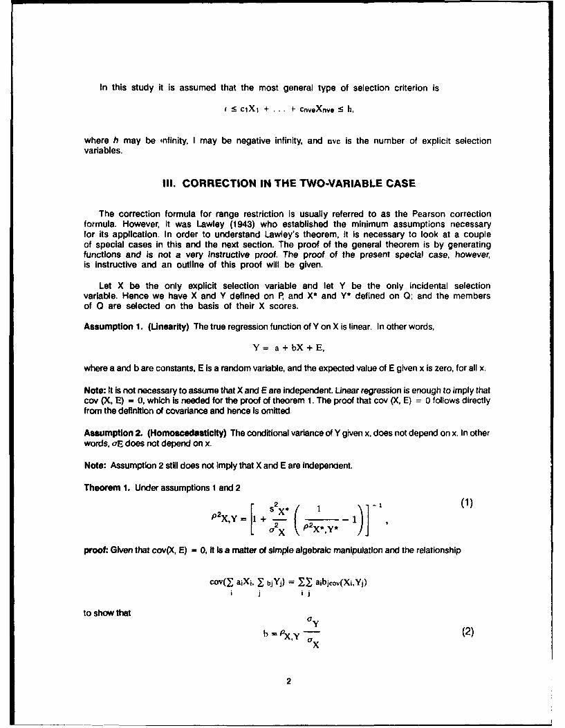
III. CORRECTION IN THE TWO-VARIABLE CASE

The correction formula for range restriction is usually referred to as the Pearson correctionformula. However, it was Lawley (1943) who established the minimum assumptions necessaryfor its application. In order to understand Lawley's theorem, it is necessary to look at a coupleof special cases in this and the next section. The proof of the general theorem is by generatingfunctions and is not a very instructive proof. The proof of the present special case, however,is instructive and an outline of this proof will be given.

Let X be the only explicit selection variable and let Y be the only incidental selectionvariable. Hence we have X and Y defined on P, and X* and Y* defined on 0; and the membersof 0 are selected on the basis of their X scores.

Assumption 1. (Unearity) The true regression function of Y on X is linear. In other words,

Y= a+bX+E,

where a and b are constants, E is a random variable, and the expected value of E given x is zero, for all x.

Note: It is not necessary to assume that X and E are independent. Linear regression is enough to imply thatcov (X, E) = 0, which Is needed for the proof of theorem 1. The proof that cov (X, E) = 0 follows directlyfrom the definition of covariance and hence is omitted.

Assumption 2. (Homoscedasticity) The conditional variance of Y given x, does not depend on x. In other

words, aE does not depend on x.

Note: Assumption 2 still does not imply that X and E are independent.

Theorem 1. Under assumptions 1 and 2

a2X P2X*,Y*rY + ( 1

proof: Given that cov(X, E) = 0, it is a matter of simple algebraic manipulation and the relationship

cov(7 aiXi, .bjYj) = 1 aibjcov(Xi,Yj)i j j

to show that

a x Y (2)ax

2

• E = a2y (1 - P2 XY). (3)

But now assur ption 1 and Equation 2 imply that

ay cry*

SPX*,Y* - (4)XY- .. X

while assumption 2 and Equation 3 imply that

o (1 ,p2 X,y) = c2y* (1 p2X*,y*).)

These two equations are exactly equivalent to the conclusion of the theorem. That is to say, you get theconclusion by solving for o2 y In Equation 4, putting that in Equation 5 and solving forPx y .

It is important to understand that the conclusion depends exactly on linearity andhomoscedasticity and the fact that Y is not explicitly restricted. No assumption of normality isneeded. The population parameters that appear on the right side of the formula will, of course,not be known and so the statistic based on this theorem becomes

which is the Pearson statistic for two variables. The sampling distribution of this statistic does depend onthe joint distribution of X and Y. The simulation program described later assumes that this distribution Is thebivariate normal. From looking at a few examples using that program it appears that the corrected statisticis always a slight underestimate. In the cases examined, this downward bias seems to be so small that itcould easily be ignored.

Notice that if c22X* < a 2 X, a it will be for the type of restrictions we are considering,then P 2X*,y* < P2X,Y- So if rX*,Y* is used ipstead of the correction formula, this givesan estimate for a parameter that is smaller than P X,U. This last statement is not true whenthere are more than two variables. This will be discussed in the next section.

The effect of range restriction on population parameters in the two-variable case is easilyvisualized. Think of a correlation coefficient as a measure of how well we can perform thefollowing task. Administer test X to two randomly chosen individuals and predict which of theseindividuals would score highest on test Y. There are three characteristics of the joint densityfunction between X and Y that determine how well we can predict. The first Is the slope ofthe regression line. This does not change with a restriction on X. The fact that it does notchange is reflected by Equation 4, which Is part of the proof of theorem 1. It is obvious thata greater slope leads to greater chance of successfully predicting which individual will have thelarger Y score. The second Is oaE This does not change with a restriction in X. The fact thatit does not change is reflected in Equation 5, which is the other significant equation in theproof of theorem 1. It is clear that a smaller oaE leads to a greater chance of picking thecorrect individual. The way this is reflected in the equation

axPX,Y = b_

3ry

3

is that if OE is made smaller without changing oX or b, then ay will become smaller. The third factor is thevariance of X. It is clear that we have a better chance of choosing the correct individual if the X values ofrandomly chosen people are spread out rather than being packed together. This isthe factor that is depressedas a result of selection. As already mentioned, for the type of selection in common use the variance of X* isalways smaller than the variance of X. Hence in the two-variable case, selection always causes under-estimation of the correlation coefficient If the correction formula is not used.

One of the benefits of presenting a proof of theorem 1 and then discussing how the threefactors affect correlation coefficients is that one can see how correlation estimation dependson linearity and homoscedasticity. If one or both of these conditions fail drastically, then it willbe very difficult to get a decent estimate. A few comments about this problem will be madeat the end of this paper.

IV. THREE VARIABLES WITH ONE EXPLICITLY RESTRICTED

Let X be the explicit selection variable and let Y and Z be incidental selection variables. Y

is the criterion or dependent variable and X and Z are the independent or predictor variables.

Assumption 1. The true regressions of Z on X, and Y on X, are linear.

Assumption 2. The variance of Y given X, the variance of Z given X, and the covariance of Z and Y givenX, do not depend on X.

Theorem 2: Under assumptions 1 and 2

"Y y . . . .ix- , 'or×. \ rX

P2.Y ;.c 4-

This correction formula is slightly more complex and it permits the construction of exampleswhere the correlation in the restricted population is larger than the correlation in the unrestrictedpopulation. Levin (1972) refers to these cases as "Pseudo-Paradoxical." The terminology probablystems from the fact that it Is widely assumed in the literature that restriction always causes anunderestimate. This would certainly be expected on the basis of our discussion in the two-variablecase. Notice that with the formula appearing in theorem 2 and a little algebra it is easy tocharacterize these "Pseudo-Paradoxical" situations In the three-variable case. In these cases theuncorrected estimation is an overestimation. Taking examples from Levin (1972), the correctionprocedure was applied and the simulation showed each time that the corrected value was verygood. It seemed that the corrected estimate was slightly low in each case but the estimatewas so close that this low estimation might not be a real effect. In any case the bias appearsto be so slight that it is not practically significant. The interesting fact is that the correctionstatistic based on theorem 2 works well in these cases, at least when the joint distribution ofthe three variables is multinormal.

4

V. THE GENERAL CASE

Let X be the p-element vector of explicit selection variables, and Y the n-p element vectorof incidental selection variables on the applicant group. Y will contain one criterion variableand several predictor variables. Then X* and Y* represent the explicit and incidental selectionvariables on he selected group. Let

= [Vp, Vp,n-p]

I Vnp,p Vn-p~n-p

represent the variance-covariance matrix for X*, Y*. The first p rows and columns refer to thecomponents of X*. So Vp,p is the variance-covariance matrix of X*, Vn.p,n- p is thevariance-covariance matrix for Y*, Vpn- p gives the covariances between X* and Y*, and Vn.p, pis the transpose of Vp,n-p. In this discussion, V refers to selected data and W refers to applicantdata. In our application, V will be the estimate of the variance-covariance of all tests and it isbased on selected data. The restricted population consists of those who were accepted intothe organization so we have data on all tests for these people. Let

W=Wp,p Wp,n-p

[Wn.pp Wn-pn-p]

be the matrix of variance-covariance for the unselected data. We will estimate Wp,p from the data sincewe have data for the explicit selection variables on all applicants. The Wp,n.p, Wn-p,p, and Wn-p,n-p arethe matrices that we wish to know and will be given to us by the theorem. Wn.p,p is, of course, thetranspose of Wp,n.p; so, we will just give an expression for Wp,n.p when we state the theorem. The follow-ing statement of the theorem is taken from Birnbaum, Paulson, and Andrews (1950).

Assumption 1: (Linearity) For each j the true regression of Yj on X is linear.

Assumption 2: (Homoscedasticity) The conditional variance-covariance matrix of Y given X does notdepend on X

Theorem 3: Under assumptions 1 and 2

W, p,= Wpp, V -JVp.,,_p and

S= v._, _, - V _ P'(V3- I - V - W P.3V; 5 L )VP..

Lawley proved this theorem in 1943 using moment-generating functions. Both of the earliertheorems (1 and 2) are just special cases of theorem 3. With some algebraic manipulationsthe reader can verify this by writing out the entries of the matrix and comparing them with theformulas in the earlier theorems. Remember that the matrices of Lawley's theorem arevariance-covariance matrices and so should be converted to correlation coefficients for thepurposes of comparison.

Notice that the theorem says nothing about tt-e types of restrictions that are allowed.Restrictions of any type on the X variables will preserve the linearity and homoscedasticity.However, if there are explicit restriction variables that are not known and hence not includedin the equations of theorem 3, then the accuracy of the corrected statistic suffers. The conditionsspecified in Lawley's theorem are not met in this case.

5

VI. AN EXAMPLE

The following data are taken from Air Force performance measurement research records.They are the scores (Maler & Sims, 1986) on the 10 subtests of the enlistment qualificationbattery (variables 1-10) arid a performance test (variable 11) (Green & Wing, 1988). Table 1shows the correlations of these variables as observed in a sample from the restricted population.Hence they are not corrected for range restriction.

Table 1. Restricted Data

1.0000.143 1.0000.568 0.216 1.0000.381 0.244 0.537 1.0000.011 0.225 0.162 0.185 1.0000.112 0.251 0.200 0.157 0.583 1.0000.130 0.235 0.223 0.254 -.078 -.042 1.0000.371 0.381 0.271 0.192 0.244 0.320 -.125 1.0000.342 0.172 0.296 0.406 -.057 0.080 0.475 0.220 1.0000.308 -.030 0.161 0.018 -.158 -.039 0.451 -.018 0.283 1.0000.141 0.393 0.035 0.118 0.110 0.236 0.159 0.298 0.250 0.077 1.000

Table 2 shows the correlations of the first 10 variables (explicitly restricted variables) ascalculated using a sample from the unrestricted population. Pearson correction will not changethese values. They are the best estimates for the correlation coefficients between the explicitlyrestricted variables. Notice that some estimates have changed from slightly negative to significantlypositive.

Table 2. Unrestricted Data

1.0000.722 1.0000.801 0.708 1.0000.689 0.672 0.803 1.0000.524 0.627 0.617 0.608 1.0000.452 0.515 0.550 0.561 0.701 1.0000.637 0.533 0.529 0.423 0.306 0.225 1.0000.695 0.827 0.670 0.637 0.617 0.520 0.415 1.0000.695 0.684 0.593 0.521 0.408 0.336 0.741 0.600 1.0000.760 0.658 0.684 0.573 0.421 0.342 0.745 0.585 0.743 1.000

Table 3 shows the correlations presented in Table 1 after the correction procedure has beenapplied. The last row of correlations of the subtests with variable 11 have now been correctedfor range restriction. It is seen that these correlations have changed considerably in the processof being corrected for range restriction. These corrected values are the best available estimatesfor these correlation coefficients.

6

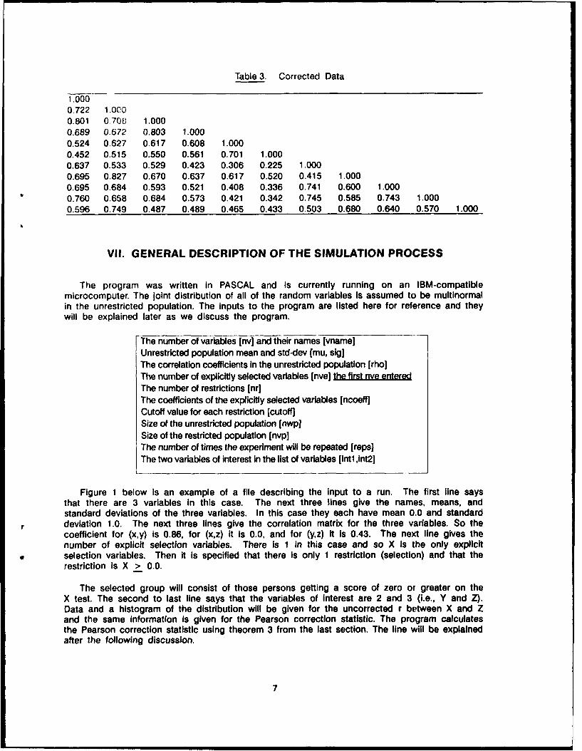
Table 3. Corrected Data

1.0000.722 1.0000.801 0.708 1.0000.689 0.672 0.803 1.0000.524 0.627 0.617 0.608 1.0000.452 0.515 0.550 0.561 0.701 1.0000.637 0.533 0.529 0.423 0.306 0.225 1.0000.695 0.827 0.670 0.637 0.617 0.520 0.415 1.0000.695 0.684 0.593 0.521 0.408 0.336 0.741 0.600 1.0000.760 0.658 0.684 0.573 0.421 0.342 0.745 0.585 0.743 1.0000.596 0.749 0.487 0.489 0.465 0.433 0.503 0.680 0.640 0.570 1.000

VII. GENERAL DESCRIPTION OF THE SIMULATION PROCESS

The program was written In PASCAL and is currently running on an IBM-compatiblemicrocomputer. The joint distribution of all of the random variables is assumed to be multinormalin the unrestricted population. The inputs to the program are listed here for reference and theywill be explained later as we discuss the program.

The number of variables [nvJ and their names [vnamelUnrestricted population mean and std-dev [mu, sig]The correlation coefficients in the unrestricted population [rho]The number of explicitly selected variables [nve] the first nve enteredThe number of restrictions [nr]The coefficients of the explicitly selected variables [ncoeff]Cutoff value for each restriction [cutoff]Size of the unrestricted population [nwp]Size of the restricted population [nvp]The number of times the experiment will be repeated [reps]The two variables of interest in the list of variables [intl ,int2]

Figure 1 below is an example of a file describing the input to a run. The first line saysthat there are 3 variables in this case. The next three lines give the names, means, andstandard deviations of the three variables. In this case they each have mean 0.0 and standarddeviation 1.0. The next three lines give the correlation matrix for the three variables. So thecoefficient for (x,y) is 0.86, for (x,z) it is 0.0, and for (yz) It Is 0.43. The next line gives thenumber of explicit selection variables. There Is 1 in this case and so X is the only explicitselection variables. Then it is specified that there is only 1 restriction (selection) and that therestriction is X > 0.0.

The selected group will consist of those persons getting a score of zero or greater on theX test. The second to last line says that the variables of interest are 2 and 3 (i.e., Y and Z).Data and a histogram of the distribution will be given for the uncorrected r between X and Zand the same information Is given for the Pearson correction statistic. The program calculatesthe Pearson correction statistic using theorem 3 from the last section. The line will be explainedafter the following discussion.

7

3x 0.0 1.0y 0.0 1.0z 0.0 1.0

1.00 0.86 0.000.86 1.00 0.430.00 0.43 1.00

1 # of explicitly restricted variables1 number of restrictions1.0 0.02 3 variables of interest1 50 100

Figure 1. An Input File.

Creating a multinormal observation is equivalent to simulating one individual. In the abovecase this means getting three values,--one for each of the three test scores X, Y, and Z. Eachmultinormal observation is part of the applicant group and is also a member of the selectedgroup if the scores satisfy all of the restrictions. For the present case this means that the scoreon the X test must be at least zero. One experiment is simulated by generating observationsuntil two conditions are satisfied. There must be at least nwp observations in the applicantgroup and there must be at least nvp observations In the selected group. For most cases weset nwp = 1 and then the only restriction is that we have at least nvp observations in theselected group. One run of the program consists of simulating reps experiments. The last lineof a file which describes a run gives, nwp, nvp and reps in that order. In Figure 1, nwp = 1,nvp = 50, and reps = 100.

When program corr begins, it will ask if the user wants to enter the data necessary todescribe a run or to"give the name of a file which contains the data in the expected format.The file in Figure 1 is called test4 and so we can just give that name to corr and the run isspecified by the input parameters in Figure 1. The reason that test4 is in the expected formatis that corr wrote the file on a previous run. It was written when corr executed and it wasspecified that data would be entered from the keyboard and that these'data were to be savedin a file named test4. Now if one were familiar with PASCAL read statements, they could usea text editor to change some of the parameters and use test4 for another run. After correxecutes, the data necessary to produce the histograms of the corrected and the uncorrectedstatistics are in two Internal files and one must run program plot which will read these internalfiles and display these data on the printer.

For each experiment corr calculates each of the following quantities.

bO and bl = the estimates of the regression parametersstatu = the uncorrected estimate of the correlation coefficientstatc = the corrected estimate of the correlation coefficient calculated

with the equations of theorem 3

Hence corr will generate reps copies of each of these parameters. In each case the twoimplied variables are Intl and int2, and the regression parameters are for int2 on Intl. In thecase of bO and bl, the only values retained are the totals so that after the reps experimentshave been generated, the mean values of these parameters may be calculated. In the case

8

tatc, each oiserved value is retained and written to the files pltu-dat and pltc.dat,

,p'cl ,, y As me'! ned earlier, the user can run plot to have all these results displayed.

VIII. PROGRAM METHODOLGY

One can see that the correction procedure, as specified in theorem 3, requires taking theinverse of a matrix. This is accomplished with the Gauss-Jordan matrix inversion algorithm Inunit matops. This unit also contains algorithms to multiply and to subtract matrices.

Unit normgen includes all of the routines necessary to generate a multinormal observationwith the correlations specified in the input file. Suppose that there are nv variables. The firststep is to generate nv Independent standard normal observations. This is accomplished byrepeated calls to algorithm p in Knuth (1969). The desired multinormal distribution results fromtaking a linear transformation of these independent standard normal observations. Thistransformation is obtained by multiplying the independent observations and the matrix A whichis defined to be that unique matrix which is upper triarigular and satisfies AAT = C. In thislast equation, AT refers to the transpose of A, and C is the variance-covarlance matrix of allvariables in the unrestricted population. For a complete discussion of this procedure, consultShreider (1966) or Johnson (1987). The matrix A is calculated by the recursive procedure solvecalled by transpar in unit normpar.

IX. RECOMMENDATIONS

Much time has been spent in writing the program; hence, most of these recommendationshave to do with proposed applications of the tool. However, based on a limited amount ofexperimentation, a few observations seem appropriate.

The correction statistic seems to work well under the conditions of the theorem. It seemsto have a downward bias but, for the cases we considered, it was always preferable to theuncorrected statistic. As can be seen from the proof of theorem 1, neither the corrected northe uncorrected statistic will be accurate if the joint distribution of all variables fails to satisfythe linearity condition or the homoscedasticity condition. After fully understanding the theorem,and a little experimentation with the simulation program, It seems likely that the best strategyis to always use the Pearson correction statistic instead of the uncorrected statistic.

There are a number of studies that could be pursued with the use of the simulation program.A plot of the sampling distribution of the Fisher Z-transformatlon of the corrected statistic lookedapproximately normal, as might be expected. The Z-transformatlon could form the basis for aprocedure that could be used to construct confidence intervals for the true correlation coefficientbased on the Pearson statistic. It might be instructive to modify the program slightly so as toallow the joint distribution of all variables to be specified In the Input. This would allow one totest the confidence intervals procedure using actual data Instead of stochastically generatedmultinormal data.

It would be useful to know how much accuracy is lost In the corrected statistic when oneor more explicit selection variables have been omitted from the model. Based on a fewexperiments, the accuracy of the corrected statistic is diminished by the omission of explicitselection variables. It would be of value to know the magnitude of this effect. This is importantsince some people still use the two- or three-variable formulas even when there Is more thanone explicit selection variable. The simulation program Is ideally suited to answer this question.

9

REFERENCES

Bimbaum, Z.W., Paulson, E., & Andrews, F.C. (1950). On the effects of selection performed on somecoordinates of a multi-dimensional population. Psychometrika, 15(2), 191-204.

Green, B.F., & Wing, H. (Eds.), (1988). Analysis of job performance measurement data. Report of aworkshop, Washington, DC: National Academy Press.

Johnson, M.E. (1987). Multivariate statistical simulation (p.49). New York: John Wiley and Sons.

Knuth, D. (1969). The art of computer programming: Vol.2. Seminumerical algorithms (p.104). Menlo Park,CA: Addison-Wesley.

Lawley, D.N. (1943). A note on Karl Pearson's selection formulae. Proceedings of the Royal Society ofEdlngburg. Sect. A. (Math & Psys. Sec.), 62, Part I, 28-30.

Levin, J. (1972). The occurence of an increase in correlation by restriction of range. Psychometrika, 37(1),93-97.

Lord, F.M., & Novick, M.R. (1968). Statistical theories of mental test scores. Menlo Park, CA:Addison-Wesley.

Maier, M.H., & Sims W.H. (1986). The ASVAB score scale: 1980 and World War II (CNR 116). Arlington, VA:Center for Naval Analysis.

Pearson, K. (1903). On the Influence of natural selection on the variability and correlation of organs. Phil.Transactions of the Royal Society A, 200, 1-66.

Shreider, Y.A. (1966). The Monte Carlo method (p. 328). Elmsford, NY: PerGamon Press.

10